AMD-stability and the classification of planetary systems.

We present here in full detail the evolution of the angular momentum deficit (AMD) during collisions as it was described in (Laskar, 2000). Since then, the AMD has been revealed to be a key parameter for the understanding of the outcome of planetary formation models. We define here the AMD-stability criterion that can be easily verified on a newly discovered planetary system. We show how AMD-stability can be used to establish a classification of the multiplanet systems in order to exhibit the planetary systems that are long-term stable because they are AMD-stable, and those that are AMD-unstable which then require some additional dynamical studies to conclude on their stability. The AMD-stability classification is applied to the 131 multiplanet systems from The Extrasolar Planet Encyclopaedia database (exoplanet.eu) for which the orbital elements are sufficiently well known.

1 Introduction

The increasing number of planetary systems has made it necessary to search for a possible classification of these planetary systems. Ideally, such a classification should not require heavy numerical analysis as it needs to be applied to large sets of systems. Some possible approaches can rely on the stability analysis of these systems, as this stability analysis is also part of the process used to consolidate the discovery of planetary systems. The stability analysis can also be considered a key part to understanding the wider question of the architecture of planetary systems. In fact, the distances between planets and other orbital characteristic distributions is one of the oldest questions in celestial mechanics, the most famous attempts to set laws for this distribution of planetary orbits being the Titius-Bode power laws (see Nieto 1972; Graner & Dubrulle 1994 for a review).

Recent research has focused on statistical analysis of observed architecture (Fabrycky et al., 2014; Lissauer et al., 2011; Mayor et al., 2011), eccentricity distribution (Moorhead et al., 2011; Shabram et al., 2016; Xie et al., 2016), or inclination distribution (Fang & Margot, 2012; Figueira et al., 2012); see Winn & Fabrycky (2015) for a review. The analysis of these observations has been compared with models of system architecture (Fang & Margot, 2013; Pu & Wu, 2015; Tremaine, 2015). These theoretical works usually use empirical criteria based on the Hill radius proposed by Gladman (1993) and refined by Chambers et al. (1996); Smith & Lissauer (2009), and Pu & Wu (2015). These criteria of stability usually multiply the Hill radius by a numerical factor $\Delta_{\mathrm{sep}}$ empirically evaluated to a value around 10. They are extensions of the analytical results on Hill spheres for the three-body problem (Marchal & Bozis, 1982). Works on chaotic motion caused by the overlap of mean motion resonances (MMR, Wisdom, 1980; Deck et al., 2013; Ramos et al., 2015) could justify the Hill-type criteria, but the results on the overlap of the MMR island are valid only for close orbits and for short-term stability.

Another approach to stability analysis is to consider the secular approximation of a planetary system. In this framework, the conservation of the semi-major axis leads to the conservation of another quantity, the angular momentum deficit (AMD; Laskar, 1997, 2000). An architecture model can be developed from this consideration (Laskar, 2000). The AMD can be interpreted as a measure of the orbits’ excitation (Laskar, 1997) that limits the planets close encounters and ensures long-term stability. Therefore a stability criterion can be derived from the semi-major axis, the masses and the AMD of a system. In addition, it can be demonstrated that the AMD decreases during inelastic collisions (see section 2.3), accounting for the gain of stability of a lower multiplicity system. Here we extend the previous analysis of (Laskar, 2000), and derive more precisely the AMD-stability criterion that can be used to establish a classification of the multiplanetary systems.

In the original letter (Laskar, 2000), the detailed computations were referred to as a preprint to be published. Although this preprint has been in nearly final form for more than a decade, and has even been provided to some researchers (Hernández-Mena & Benet, 2011), it is still unpublished. In Sects. 2 and 3 we provide the fundamental concepts of AMD, the full description, and all proofs for the model that was described in (Laskar, 2000). This material is close to the unpublished preprint. Section 4 recalls briefly the model of planetary accretion based on AMD stochastic transfers that was first presented in (Laskar, 2000). This model provides analytical expressions for the averaged systems architecture and orbital parameter distribution, depending on the initial mass distribution (Table 2).

In Sect. 5, we show how the AMD-stability criterion presented in section 3 can be used to develop a classification of planetary systems. This AMD-stability classification is then applied to a selection of 131 multiplanet systems from The Extrasolar Planet Encyclopaedia database (exoplanet.eu) with known eccentricities. Finally, in Sect. 6 we discuss our results and provide some possible extension for this work.

2 Angular momentum deficit

2.1 Planetary Hamiltonian

Let $P_{0},P_{1},\dots,P_{n}$ be $n+1$ bodies of masses $m_{0},m_{1},\dots,m_{n}$ in gravitational interaction, and let $O$ be their centre of mass. For every body $P_{i}$, we denote ${\bf u}_{i}=\overrightarrow{OP_{i}}$. In the barycentric reference frame with origin $O$, Newton’s equations of motion form a differential system of order $6(n+1)$ and can be written in Hamiltonian form using the canonical coordinates $({\bf u}_{i},{\bf\tilde{u}}_{i}=m_{i}\dot{\bf u}_{i})_{i=0,n}$ with Hamiltonian

$$H={{\displaystyle 1}\over{\displaystyle 2}}\sum_{i=0}^{n}{{\displaystyle\|{\bf\tilde{u}}_{i}\|^{2}}\over{\displaystyle m_{i}}}-\mathcal{G}\sum_{0\leq i<j}{{\displaystyle m_{i}m_{j}}\over{\displaystyle\Delta_{ij}}},$$ (1)

where $\Delta_{ij}=\|{\bf u}_{i}-{\bf u}_{j}\|$, and $\mathcal{G}$ is the constant of gravitation. The reduction of the centre of mass is achieved by using the canonical heliocentric variables of Poincaré $({\bf r}_{i},{\bf\tilde{r}}_{i})$ (Poincaré, 1905; Laskar & Robutel, 1995), defined as

$${\bf r}_{0}={\bf u}_{0};\qquad{\bf r}_{i}={\bf u}_{i}-{\bf u}_{0}\qquad\hbox{for }i\neq 0$$ (2)

$${\bf\tilde{r}}_{0}={\bf\tilde{u}}_{0}+{\bf\tilde{u}}_{1}+\cdots+{\bf\tilde{u}}_{n};\qquad{\bf\tilde{r}}_{i}={\bf\tilde{u}}_{i}\qquad\hbox{for }i\neq 0$$ (3)

This Hamiltonian can then be split into an integrable part, $H_{0}$, and a perturbation, $H_{1}$,

$$H=H_{0}+H_{1}$$ (4)

with

$$H_{0}={{\displaystyle 1}\over{\displaystyle 2}}\sum_{i=1}^{n}{{\displaystyle\|{\bf\tilde{r}}_{i}\|^{2}}\over{\displaystyle m_{i}}}-\mathcal{G}\sum_{i=1}^{n}{{\displaystyle m_{0}m_{i}}\over{\displaystyle r_{i}}}$$ (5)

and

$$H_{1}={{\displaystyle 1}\over{\displaystyle 2}}{{\displaystyle\|{\bf\tilde{u}}_{0}\|^{2}}\over{\displaystyle m_{0}}}-\mathcal{G}\sum_{1\leq i<j}{{\displaystyle m_{i}m_{j}}\over{\displaystyle\Delta_{ij}}}$$ (6)

The integrable part, $H_{0}$, is the Hamiltonian of a sum of disjoint Kepler problems of a single planet of mass $m_{i}$ around a fixed Sun of mass $m_{0}$. A set of adapted variables for $H_{0}$ will thus be given by the elliptical elements, $(a_{k},e_{k},i_{k},\lambda_{k},\varpi_{k},\Omega_{k})$, where $a_{k}$ is the semi-major axis, $e_{k}$ the eccentricity, $i_{k}$ the inclination, $\lambda_{k}$ the mean longitude, $\varpi_{k}$ the longitude of the perihelion, and $\Omega_{k}$ the longitude of the node. They are defined as the elliptical elements associated to the Hamiltonian

$$H_{0k}={{\displaystyle 1}\over{\displaystyle 2}}{{\displaystyle\|{\bf\tilde{r}}_{k}\|^{2}}\over{\displaystyle m_{k}}}-\mu{{\displaystyle m_{k}}\over{\displaystyle r_{k}}}$$ (7)

with $\mu=\mathcal{G}m_{0}$.

2.2 Angular momentum deficit (AMD)

The total linear momentum of the system is null in the barycentric reference frame

$$L=\sum_{i=0}^{n}m_{i}\dot{\bf u}_{i}=\sum_{i=0}^{n}{\bf\tilde{u}}_{i}={\bf\tilde{r}}_{0}=0\ .$$ (8)

Let ${\bf G}$ be the total angular momentum. Its expression is not changed by the linear symplectic change of variable $({\bf u},{\bf\tilde{u}})\longrightarrow({\bf r},{\bf\tilde{r}})$. We have thus

$${\bf G}=\sum_{i=0}^{n}{\bf u}_{i}\,\wedge{\bf\tilde{u}}_{i}=\sum_{i=1}^{n}{\bf r}_{i}\,\wedge{\bf\tilde{r}}_{i}$$ (9)

When expressed in heliocentric variables, the angular momentum is thus the sum of the angular momentum of the Keplerian problems of the unperturbed Hamiltonian $H_{0}$. In particular, if the angular momentum direction is assumed to be the axis $z$, the norm of the angular momentum is

$$G=\sum_{k=1}^{n}\Lambda_{k}\sqrt{1-e_{k}^{2}}\cos i_{k},$$ (10)

where $\Lambda_{k}=m_{k}\sqrt{\mu\,a_{k}}$. For such a system, the AMD is defined as the difference between the norm of the angular momentum of a coplanar and circular system with the same semi-major axis values and the norm of the angular momentum ($G$), i.e. (Laskar, 1997, 2000)

$$C=\sum_{k=1}^{n}\Lambda_{k}\left(1-\sqrt{1-e_{k}^{2}}\cos i_{k}\right)$$ (11)

2.3 AMD and collision of orbits

The instabilities of a planetary system often result in a modification of its architecture. A planet can be ejected from the system or can fall into the star; in both cases this results in a loss of AMD for the system. The outcome of the AMD after a planetary collisions is less trivial and needs to be computed. Assume that among our $n+1$ bodies, the (totally inelastic) collision of two bodies of masses $m_{1}$ and $m_{2}$, and orbits ${\cal O}_{1},{\cal O}_{2}$ occurs, forming a new body $(m_{3},{\cal O}_{3})$. During this collision we assume that the other bodies are not affected. The mass is conserved

$$m_{3}=m_{1}+m_{2},$$ (12)

and the linear momentum in the barycentric reference frame is conserved so ${\bf\tilde{u}}_{3}={\bf\tilde{u}}_{1}+{\bf\tilde{u}}_{2}$, and also

$${\bf\tilde{r}}_{3}={\bf\tilde{r}}_{1}+{\bf\tilde{r}}_{2}\ ;$$ (13)

On the other hand, ${\bf r}_{3}={\bf r}_{1}={\bf r}_{2}$ at the time of the collision, so the angular momentum is also conserved

$${\bf r}_{3}\,\wedge{\bf\tilde{r}}_{3}={\bf r}_{1}\,\wedge{\bf\tilde{r}}_{1}+{\bf r}_{2}\,\wedge{\bf\tilde{r}}_{2}$$ (14)

It should be noted that the transformation of the orbits $(m_{1},{\cal O}_{1})+(m_{2},{\cal O}_{2})\longrightarrow(m_{3},{\cal O}_{3})$ during the collision is perfectly defined by Eqs. (12, 13). The problem which remains is to compute the evolution of the elliptical elements during the collision.

2.3.1 Energy evolution during collision

Just before the collision, we assume that the orbits $(m_{1},{\cal O}_{1})$ and $(m_{2},{\cal O}_{2})$ are elliptical heliocentric orbits. At the time of the collision, only these two bodies are involved and the other bodies are not affected. The evolution of the orbits are thus given by the conservation laws (12, 13). The Keplerian energy of each particle is

$$h_{i}={{\displaystyle 1}\over{\displaystyle 2}}{{\displaystyle\|{\bf\tilde{r}}_{i}\|^{2}}\over{\displaystyle m_{i}}}-\mu{{\displaystyle m_{i}}\over{\displaystyle r_{i}}}=-\mu{{\displaystyle m_{i}}\over{\displaystyle 2a_{i}}}$$ (15)

At collision, we have ${\bf r}_{1}={\bf r}_{2}={\bf r}_{3}={\bf r}$; we have thus the conservation of the potential energy

$$-\mu{{\displaystyle m_{3}}\over{\displaystyle r_{3}}}=-\mu{{\displaystyle m_{1}+m_{2}}\over{\displaystyle r}}=-\mu{{\displaystyle m_{1}}\over{\displaystyle r_{1}}}-\mu{{\displaystyle m_{2}}\over{\displaystyle r_{2}}}\ .$$ (16)

The change of Keplerian energy is thus given by the change of kinetic energy

$$\delta h=h_{3}-h_{1}-h_{2}={{\displaystyle 1}\over{\displaystyle 2}}{{\displaystyle\|{\bf\tilde{r}}_{3}\|^{2}}\over{\displaystyle m_{3}}}-{{\displaystyle 1}\over{\displaystyle 2}}{{\displaystyle\|{\bf\tilde{r}}_{1}\|^{2}}\over{\displaystyle m_{1}}}-{{\displaystyle 1}\over{\displaystyle 2}}{{\displaystyle\|{\bf\tilde{r}}_{2}\|^{2}}\over{\displaystyle m_{2}}};$$ (17)

that is, with Eqs. (12, 13),

$${\displaystyle 2m_{1}m_{2}m_{3}\delta h} {\displaystyle{\phantom{0}}=m_{1}m_{2}({\bf\tilde{r}}_{1}+{\bf\tilde{r}}_{2})^{2}-m_{2}(m_{1}+m_{2}){\bf\tilde{r}}_{1}^{2}-m_{1}(m_{1}+m_{2}){\bf\tilde{r}}_{2}^{2}} {\displaystyle{\phantom{0}}=-m_{2}^{2}{\bf\tilde{r}}_{1}^{2}-m_{1}^{2}{\bf\tilde{r}}_{2}^{2}+2m_{1}m_{2}{\bf\tilde{r}}_{1}\cdot{\bf\tilde{r}}_{2}} {\displaystyle{\phantom{0}}=-(m_{2}{\bf\tilde{r}}_{1}-m_{1}{\bf\tilde{r}}_{2})^{2}} {\displaystyle{\phantom{0}}\leq 0}$$ (18)

Thus, the Keplerian energy of the system decreases during collision. Part of the kinetic energy is dispelled during the collision. As expected, there is no loss of energy when $m_{2}{\bf\tilde{r}}_{1}=m_{1}{\bf\tilde{r}}_{2}$, that is, as $m_{1}m_{2}\neq 0$, when $\dot{\bf u}_{1}=\dot{\bf u}_{2}$. As an immediate consequence of the decrease of energy during the collision, we have

$${{\displaystyle 1}\over{\displaystyle a_{3}}}\geq{{\displaystyle m}\over{\displaystyle a_{1}}}+{{\displaystyle 1-m}\over{\displaystyle a_{2}}}$$ (19)

with

$$m={{\displaystyle m_{1}}\over{\displaystyle m_{1}+m_{2}}}={{\displaystyle m_{1}}\over{\displaystyle m_{3}}}$$ (20)

2.3.2 AMD evolution during collision

Let $f(x)=1/\sqrt{x}$. As $f^{\prime}(x)<0$ and $f^{\prime\prime}(x)>0$, we have, as $f$ is decreasing and convex,

$$f\left({{\displaystyle 1}\over{\displaystyle a_{3}}}\right)\leq f\left({{\displaystyle m}\over{\displaystyle a_{1}}}+{{\displaystyle 1-m}\over{\displaystyle a_{2}}}\right)\leq mf\left({{\displaystyle 1}\over{\displaystyle a_{1}}}\right)+(1-m)f\left({{\displaystyle 1}\over{\displaystyle a_{2}}}\right)$$ (21)

thus

$$m_{3}\sqrt{a_{3}}\leq m_{1}\sqrt{a_{1}}+m_{2}\sqrt{a_{2}}$$ (22)

During the collision, the angular momentum is conserved (14), and so is the conservation of its normal component, that is

$${\displaystyle m_{3}\sqrt{\mu a_{3}}\sqrt{1-e_{3}^{2}}\cos i_{3}=} {\displaystyle m_{1}\sqrt{\mu a_{1}}\sqrt{1-e_{1}^{2}}\cos i_{1}+m_{2}\sqrt{\mu a_{2}}\sqrt{1-e_{2}^{2}}\cos i_{2}\ .}$$ (23)

We deduce that in all circumstances we have a decrease of the angular momentum deficit during the collision, that is

$$C_{3}\leq C_{1}+C_{2}$$ (24)

with

$$C_{k}=m_{k}\sqrt{\mu a_{k}}(1-\sqrt{1-e_{k}^{2}}\cos i_{k})\qquad{(k=1,3)}$$ (25)

The equality can hold in (24) only if $m_{1}=0$, $m_{2}=0$, or $a_{1}=a_{2}$ and ${\bf\dot{u}}_{1}={\bf\dot{u}}_{2}$, that is when one of the bodies is massless, or when the two bodies are on the same orbit and at the same position (at the time of the collision, we also have ${\bf r}_{1}={\bf r}_{2}$).

The diminution of AMD during collisions acts as a stabilisation of the system. A parallel can be made with thermodynamics, the AMD behaving for the orbits like the kinetic energy for the molecules of a perfect gas. The loss of AMD during collisions can thus be interpreted as a cooling of the system.

3 AMD-stability

We say that a planetary system is AMD-stable if the angular momentum deficit (AMD) amount in the system is not sufficient to allow for planetary collisions. As this quantity is conserved in the secular system at all orders (see Appendix B), we conjecture that in absence of short period resonances, the AMD-stability ensures the practical long-term stability of the system. Thus for an AMD-stable system, short-term stability will imply long-term stability.

The condition of AMD-stability is obtained when the orbits of two planets of semi-major axis $a,a^{\prime}$ cannot intersect under the assumption that the total AMD $C$ has been absorbed by these two planets. It can be seen easily that the limit condition of collision is obtained in the planar case and can thus be written as

$$a(1+e)=a^{\prime}(1-e^{\prime})$$ (26)

$$m\sqrt{\mu a}(1-\sqrt{1-e^{2}})+m^{\prime}\sqrt{\mu a^{\prime}}(1-\sqrt{1-e^{\prime 2}})=C,$$ (27)

where $(m,a,e)$ are the parameters of the inner orbit and $(m^{\prime},a^{\prime},e^{\prime})$ those of the outer orbit ($a\leq a^{\prime}$).

3.1 Collisional condition

We assume that $a,a^{\prime},m,m^{\prime}$ are non-zero. Denoting $\alpha=a/a^{\prime}$, $\gamma=m/m^{\prime}$, the system in Eq. (27) becomes

$${\mathcal{D}}(e,e^{\prime}) =\alpha e+e^{\prime}-1+\alpha=0$$ (28)

(33)

with $\Lambda^{\prime}=m^{\prime}\sqrt{\mu a^{\prime}}$, and where ${\mathscr{C}}(e,e^{\prime})=C/\Lambda^{\prime}$ is called the relative AMD. As $e$ and $e^{\prime}$ are planetary eccentricities, we also have

$$0\leq e\leq 1\ ;\qquad 0\leq e^{\prime}\leq 1\ .$$ (34)

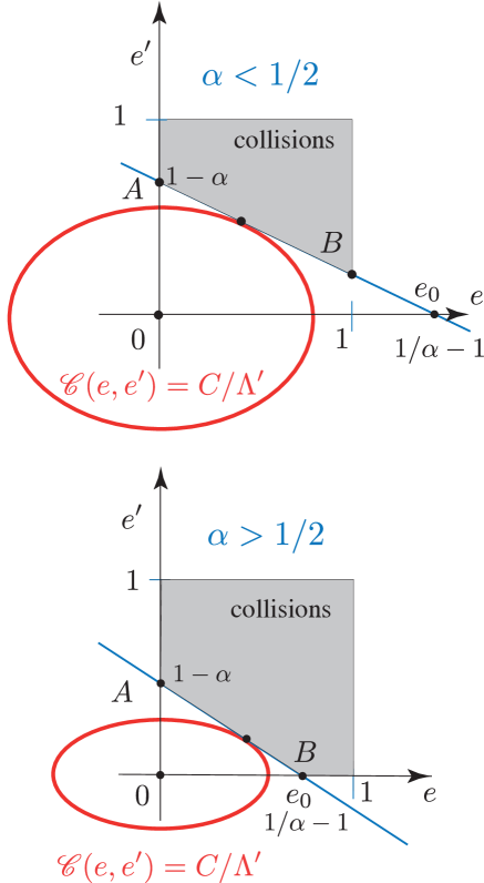
Figure 1: Collision conditions for $e_{0}=1/\alpha-1$. Case (a): $\alpha<1/2\Longleftrightarrow e_{0}>1$. Case (b): $\alpha>1/2\Longleftrightarrow e_{0}<1$. Collisions can only occur in the shaded region.

The set of collisional conditions (Eqs. 28, 33, 34) can be solved using Lagrange multipliers. We are looking for the minimum value of the relative AMD ${\mathscr{C}}(e,e^{\prime})$ (33) for which the collision condition (28) is satisfied. These conditions are visualised in the $(e,e^{\prime})$ plane in Fig. 1. The collision condition (28) corresponds to the segment $AB$ of Fig. 1. The domain of collisions is limited by the conditions (34). For $e=0$, we have $e^{\prime}_{0}=1-\alpha<1$, and the intersection of the collision line with the axis $e^{\prime}=0$ is obtained for $e_{0}={1}/{\alpha}-1$. This value can be greater or smaller than $1$ depending on the value of $\alpha$. We have thus the different cases (Fig. 1)

$$(a)\quad\alpha <{{\displaystyle 1}\over{\displaystyle 2}}\Longleftrightarrow e_{0}>1\quad \hbox{and}\quad e\leq 1$$ (35)

$$(b)\quad\alpha >{{\displaystyle 1}\over{\displaystyle 2}}\Longleftrightarrow e_{0}<1\quad \hbox{and}\quad e<e_{0}$$ (36)

and the limit case $\alpha=1/2$, for which $e_{0}=1$. In all cases, the Lagrange multipliers condition is written

$$\lambda\nabla{\mathcal{D}}(e,e^{\prime})=\nabla{\mathscr{C}}(e,e^{\prime}),$$ (37)

which gives

$${{\displaystyle\sqrt{1-e^{\prime 2}}}\over{\displaystyle e^{\prime}}}={{\displaystyle\sqrt{\alpha}}\over{\displaystyle\gamma}}{{\displaystyle\sqrt{1-e^{2}}}\over{\displaystyle e}}$$ (38)

This relation allows $e^{\prime}$ to be eliminated in the collision condition (28), which becomes an equation in the single variable $e$, and parameters $(\alpha,\gamma)$:

$$F(e,\alpha,\gamma)=\alpha e+{{\displaystyle\gamma e}\over{\displaystyle\sqrt{\alpha(1-e^{2})+\gamma^{2}e^{2}}}}-1+\alpha=0.$$ (39)

Here $F(e,a,\gamma)$ is properly defined for $(e,a,\gamma)$ in the domain $D_{e,\alpha,\gamma}$ defined by $e\in[0,1],\alpha\in]0,1],\gamma\in]0,+\infty[$, as in this domain, $1-e^{2}+\gamma^{2}e^{2}/\alpha>0$. We also have

$${{\displaystyle\partial F}\over{\displaystyle\partial e}}(e,\alpha,\gamma)=\alpha+{{\displaystyle\alpha\gamma}\over{\displaystyle\left(\alpha(1-e^{2})+\gamma^{2}e^{2}\right)^{3/2}}}\ .$$ (40)

Thus, ${{\displaystyle\partial F}\over{\displaystyle\partial e}}(e,\alpha,\gamma)>0$ on the domain $D_{e,\alpha,\gamma}$ and $F(e,\alpha,\gamma)$ is strictly increasing with respect to $e$ for $e\in[0,1]$. Moreover, as $0<\alpha<1$,

$$F(0,\alpha,\gamma)=-1+\alpha<0\ ;\qquad F(1,\alpha,\gamma)=2\alpha>0\ ;$$ (41)

and

$$F(e_{0},\alpha,\gamma)={{\displaystyle\gamma e_{0}}\over{\displaystyle\sqrt{\alpha\left(1-e_{0}^{2}\right)+\gamma^{2}e_{0}^{2}}}}>0\ .$$ (42)

The equation of collision (39) thus always has a single solution $e_{c}$ in the interval $]0,\min(1,e_{0})[$. This ensures that this critical value of $e$ will fulfil the condition (34). The corresponding value of the relative AMD $C_{c}(\alpha,\gamma)={\mathscr{C}}(e_{c},e^{\prime}_{c})$ is then obtained through (33).

3.2 Critical AMD $C_{c}(\alpha,\gamma)$

We have thus demonstrated that for a given pair of ratios of semi-major axes and masses, $(\alpha,\gamma)$, there is always a unique critical value $C_{c}(\alpha,\gamma)$ of the relative AMD ${\mathscr{C}}=C/\Lambda^{\prime}$ which defines the AMD-stability. The system of two planets is AMD-stable if and only if

$${\mathscr{C}}={{\displaystyle C}\over{\displaystyle\Lambda^{\prime}}}<C_{c}(\alpha,\gamma)\ .$$ (43)

The value of the critical AMD $C_{c}(\alpha,\gamma)$ is obtained by computing first the critical eccentricity $e_{c}(\alpha,\gamma)$ which is the unique solution of the collisional equation (39) in the interval $[0,1]$. The critical AMD is then $C_{c}(\alpha,\gamma)={\mathscr{C}}(e_{c},e^{\prime}_{c})$ (Eq.33), where the critical value $e^{\prime}_{c}$ is obtained from $e_{c}$ through Eq. 28. It is important to note that the critical AMD, and thus the AMD-stability condition, depends only on $(\alpha,\gamma)$.

3.3 Behaviour of the critical AMD

Table 1: Special values of $C_{c}(\alpha,\gamma)$. The detail of the computations is provided in Appendix C.

$\gamma$	$\alpha$	$e_{c}(\alpha,\gamma)$	$e^{\prime}_{c}(\alpha,\gamma)$	$C_{c}((\alpha,\gamma)$
$\gamma\rightarrow 0$	$\alpha<1/2$	$1-2{{\displaystyle 1-\alpha}\over{\displaystyle(1-2\alpha)^{2}}}\gamma^{2}$	$1-2\alpha+2{{\displaystyle\alpha(1-\alpha)}\over{\displaystyle(1-2\alpha)^{2}}}\gamma^{2}$	$1-2\sqrt{\alpha(1-\alpha)}+\sqrt{\alpha}\gamma$
$\gamma\rightarrow 0$	$\alpha=1/2$	$1-(4\gamma)^{2/3}$	$2^{1/3}\gamma^{2/3}$	${{\displaystyle\gamma}\over{\displaystyle\sqrt{2}}}$
$\gamma\rightarrow 0$	$\alpha>1/2$	$e_{0}-{{\displaystyle e_{0}}\over{\displaystyle\sqrt{\alpha(2\alpha-1)}}}\gamma$	${{\displaystyle\sqrt{\alpha}e_{0}\gamma}\over{\displaystyle\sqrt{2\alpha-1}}}$	$\left(\sqrt{\alpha}-\sqrt{2-{{1}\over{\alpha}}}\right)\gamma$
$\gamma\rightarrow+\infty$	$0<\alpha<1$	${{\displaystyle 1}\over{\displaystyle\gamma}}{{\displaystyle 1-\alpha}\over{\displaystyle\sqrt{2-\alpha}}}$	$1-\alpha-{{\displaystyle 1}\over{\displaystyle\gamma}}{{\displaystyle\alpha(1-\alpha)}\over{\displaystyle\sqrt{2-\alpha}}}$	$1-\sqrt{\alpha(2-\alpha)}-{{\displaystyle\sqrt{\alpha}(1-\alpha)^{2}}\over{\displaystyle 2-\alpha}}{{\displaystyle 1}\over{\displaystyle\gamma}}$
$1$	$0\leq\alpha\leq 1$	${{\displaystyle 1-\sqrt{1-\alpha+\alpha^{2}}}\over{\displaystyle\alpha}}$	$\sqrt{1-\alpha+\alpha^{2}}-\alpha$	$1+\sqrt{\alpha}-{{\displaystyle\sqrt{\alpha-2+2\sqrt{1-\alpha+\alpha^{2}}}}\over{\displaystyle\sqrt{\alpha}}}$
				$-\sqrt{\alpha}\sqrt{1-2\alpha+2\sqrt{1-\alpha+\alpha^{2}}}$
$\sqrt{\alpha}$	$0\leq\alpha\leq 1$	${{\displaystyle 1-\alpha}\over{\displaystyle 1+\alpha}}$	${{\displaystyle 1-\alpha}\over{\displaystyle 1+\alpha}}$	$(1-\sqrt{\alpha})^{2}$

We now analyse the general properties of the critical AMD function $C_{c}(\alpha,\gamma)$. As ${{\partial F}\over{\partial e}}(e,\alpha,\gamma)>0$, we can apply the implicit function theorem to the domain $D_{e,\alpha,\gamma}$, which then ensures that the solution of the collision equation (39), $e_{c}(\alpha,\gamma)$, is a continuous function of $\gamma$ (and even analytic for $\gamma\in]0,+\infty[$). Moreover, on $D_{e,\alpha,\gamma}$,

$${{\displaystyle\partial F}\over{\displaystyle\partial\gamma}}(e,\alpha,\gamma)={{\displaystyle\alpha e\left(1-e^{2}\right)}\over{\displaystyle\left(\alpha\left(1-e^{2}\right)+\gamma^{2}e^{2}\right)^{3/2}}}\geq 0\ .$$ (44)

We also have

$${{\displaystyle\partial e_{c}}\over{\displaystyle\partial\gamma}}(\alpha,\gamma)=-{{\displaystyle e_{c}\left(1-e_{c}^{2}\right)}\over{\displaystyle\left(\alpha\left(1-e_{c}^{2}\right)+\gamma^{2}e_{c}^{2}\right)^{3/2}+\gamma}}\leq 0,$$ (45)

and $e_{c}(\alpha,\gamma)$ is a decreasing function of $\gamma$. For any given values of the semi-major axes ratio $\alpha$, and masses $\gamma$, we can thus find the critical value $C_{c}(\alpha,\gamma)$ which allows for a collision (43). For the critical value $C_{c}(\alpha,\gamma)$, a single solution corresponds to the tangency condition (Fig. 1), and this solution is obtained at the critical value $e_{c}(\alpha,\gamma)$ for the eccentricity of the orbit ${\cal O}$. The values of the critical relative AMD $C_{c}(\alpha,\gamma)$ are plotted in Figure 2 versus $\alpha$, for different values of $\gamma$. Deriving Eq. 33 with respect to $\gamma$, one obtains

$${\displaystyle{{\displaystyle\partial{\mathscr{C}}}\over{\displaystyle\partial\gamma}}=} {\displaystyle\sqrt{\alpha}\left(1-\sqrt{1-e^{2}}\right)} {\displaystyle+\gamma\sqrt{\alpha}{{\displaystyle e}\over{\displaystyle\sqrt{1-e^{2}}}}{{\displaystyle\partial e}\over{\displaystyle\partial\gamma}}+{{\displaystyle e^{\prime}}\over{\displaystyle\sqrt{1-e^{\prime 2}}}}{{\displaystyle\partial e^{\prime}}\over{\displaystyle\partial\gamma}}\ .}$$ (46)

Using the two relations (28, 38), this reduces to

$${{\displaystyle\partial C_{c}(\alpha,\gamma)}\over{\displaystyle\partial\gamma}}=\sqrt{\alpha}\left(1-\sqrt{1-e_{c}^{2}}\right)>0$$ (47)

Thus $C_{c}(\alpha,\gamma)$ strictly increases with $\gamma$. In the same way

$${{\displaystyle\partial C_{c}(\alpha,\gamma)}\over{\displaystyle\partial\alpha}}={{\displaystyle\gamma}\over{\displaystyle 2\sqrt{\alpha}}}\left(1-{{\displaystyle\left(1+e_{c}^{2}\right)}\over{\displaystyle\sqrt{1-e_{c}^{2}}}}\right)<0$$ (48)

and $C_{c}(\alpha,\gamma)$ decreases with $\alpha$.

Figure 2: Values of $C_{c}(\alpha,\gamma)$ vs. $\alpha$ for the different $\gamma$ values for which an explicit expression of $C_{c}(\alpha,\gamma)$ is obtained.

Now that the general behaviour of the critical AMD $C_{c}(\alpha,\gamma)$ is known, we can specify its explicit expression in a few special cases that are displayed in Table 1. The computations and the higher order developments can be found in Appendix C.

A development of $C_{c}(\alpha,\gamma)$ for $\alpha\longrightarrow 1$ can also be obtained (see Appendix C). With $\eta=1-\alpha$, we have

$$C_{c}(\alpha,\gamma)\sim{{\displaystyle\gamma}\over{\displaystyle\gamma+1}}{{\displaystyle\eta^{2}}\over{\displaystyle 2}}+\mathrm{O}(\eta^{3})\ .$$ (49)

We now present two applications of the AMD-stability, the formation of planetary systems, and a classification of observed planetary systems.

4 AMD model of planet formation

Once the disc has been depleted, the last phase of terrestrial planet formation begins with a disc composed of planetary embryos and planetesimals (Morbidelli et al., 2012). In numerical simulations of this phase, the AMD has been used as a statistical measure for comparison with the inner solar system (Chambers, 2001). In this part, we recall the very simple model of embryo accretion described in Laskar (2000) interpreting the $N$-body dynamics as AMD-exchange.

4.1 Collisional evolution

So far we have not made special simplifications, and the model simply preserves the mass and the momentum in the barycentric reference frame. We make an additional assumption here: between collisions, the evolution of the orbits is similar to the evolution they would have in the averaged system in the presence of chaotic behaviour. The orbital parameters will thus evolve in a limited manner, with a stochastic diffusion process, bounded by the conservation of the total AMD. As shown in section 2.3, during a collision the AMD decreases (eq. 24). We assume the collisions to be totally inelastic with perfect merging. Indeed, Kokubo & Genda (2010) and Chambers (2013) have shown that the detailed mechanisms of collisions, such as the possibilities of hit-and-run or fragmentation of embryos, barely change the final architecture of simulated systems. The total AMD of the system will thus be constant between collisions, and will decrease during collisions. On the other hand, the AMD for a particle is of the order of ${{1}\over{2}}m\sqrt{a}e^{2}$. As the mass of the particle increases, its excursion in eccentricity will be more limited, and fewer collisions will be possible. The collisions will stop when the total AMD of the system is too small to allow for planetary collisions.

In the accretion process, we consider a planetesimal of semi-major axis $a$ and its immediate neighbour, defined as the planetesimal with semi-major axis $a^{\prime}$, such that there is no other planetesimal with semi-major axis between $a$ and $a^{\prime}$. In this case we can assume that $\alpha$ is close to $1$ and, as explained in Appendix C, we use an approximation of the critical AMD value $C_{c}(\alpha,\gamma)$:

$$C_{c1}(\alpha,\gamma)=k(\gamma)\left({{\displaystyle\delta_{a}}\over{\displaystyle a}}\right)^{2},$$ (50)

where $\delta_{a}=a^{\prime}-a$ and $k(\gamma)=\gamma/(2(\gamma+1))$ .

4.2 AMD-stable planetary distribution

In this section, we search for the laws followed by the planetary distribution of a model formed following the above assumptions. We thus start from an arbitrary distribution of mass of planetesimals $\rho(a)$, and let the system evolve under the previous rules. We search for the condition of AMD-stable planetary systems, obtained by random accretion of planetesimals. This condition requires that the final AMD value cannot allow for planetary crossing among the planets. Let $C$ be the value of the AMD at the end of the accretion process. If we consider the planetesimal of semi-major axis $a$, its mass will continue to increase by accretion with a body of semi-major axis $a^{\prime}>a$, as long as

$${\mathscr{C}}={{\displaystyle C}\over{\displaystyle\Lambda^{\prime}}}\geq C_{c1}=k\left({{\displaystyle\delta_{a}}\over{\displaystyle a}}\right)^{2}$$ (51)

The initial linear density of mass is $\rho(a)$. As $a^{\prime}$ is the closest neighbour to $a$, we can assume that all the planetesimals initially between $a$ and $a^{\prime}$ have been absorbed by the two bodies of mass $m(a)$ and $m(a^{\prime})$. At first order with respect to $\delta_{a}/a$, we have thus

$$m(a^{\prime})\sim m(a)\sim\rho(a)\delta_{a},$$ (52)

and from (51) at the limiting case we have

$${{\displaystyle{\tilde{C}}}\over{\displaystyle\delta_{a}\rho(a)\sqrt{a}}}=k\left({{\displaystyle\delta_{a}}\over{\displaystyle a}}\right)^{2},$$ (53)

where ${\tilde{C}}=C/\sqrt{\mu}$. We have thus

$$\delta_{a}=\left({{\displaystyle{\tilde{C}}}\over{\displaystyle k}}\right)^{1/3}a^{1/2}\rho^{-1/3},$$ (54)

and from (52)

$$m(a)=\left({{\displaystyle{\tilde{C}}}\over{\displaystyle k}}\right)^{1/3}a^{1/2}\rho^{2/3}.$$ (55)

4.3 Scaling laws with initial mass distribution $\rho(a)\propto a^{p}$.

Using the previous relations, we can compute the resulting systems for various initial mass distribution, in particular for $\rho(a)=\zeta a^{p}$. From equation (55), we obtain for two consecutive planets

$${{\displaystyle m}\over{\displaystyle m^{\prime}}}=\alpha^{1/2}\left({{\displaystyle\rho(a)}\over{\displaystyle\rho(a^{\prime})}}\right)^{2/3}=\alpha^{{{1}\over{2}}+{{2}\over{3}}p}$$ (56)

and from Eq. (50), as $\lim_{\alpha\longrightarrow 1}\gamma=1$, we thus have $k(\gamma)={{\displaystyle 1}\over{\displaystyle 4}}$ in all cases. Relation (54) can be rewritten

$$\delta_{a}a^{{{p}\over{3}}-{{1}\over{2}}}=(4{\tilde{C}})^{1/3}\zeta^{-1/3}\delta n\,,$$ (57)

where $\delta n=1$ is the increment from planet $a$ to $a^{\prime}$. By integration, this difference relation becomes for $p\neq-{{3}\over{2}}$,

$$a^{{{2p+3}\over{6}}}=a_{0}^{{{2p+3}\over{6}}}+{{2p+3}\over{6}}\left({{\displaystyle 4{\tilde{C}}}\over{\displaystyle\zeta}}\right)^{1/3}n\ .$$ (58)

For $p=-{{3}\over{2}}$, we obtain

$$\log(a)=\log(a_{0})+(4{\tilde{C}})^{1/3}\zeta^{-1/3}n.$$ (59)

In particular, for $p=0$ (constant distribution and $\rho(a)=\zeta$), from (57), we have

$$\sqrt{a}=\sqrt{a_{0}}+\left({{\displaystyle{\tilde{C}}}\over{\displaystyle 2\zeta}}\right)^{1/3}n\ .$$ (60)

For the masses, from (55), we have for large $n$ (or if $a_{0}$ is small )

$$m(n)\sim(2{\tilde{C}}^{2}\zeta)^{1/3}n\ .$$ (61)

For $p=-3/2$, we find a power law similar to the Titius-Bode law for planetary distribution. The different expressions deduced from this model of planetary accretion are listed in Table 2.

Table 2: Planetary distribution corresponding to different initial mass distribution.

$p$	$a(n)$	$m(a)$	$m(n)$
$p\neq-3/2$	$a^{{{2p+3}\over{6}}}=a_{0}^{{{2p+3}\over{6}}}+{{\displaystyle 2p+3}\over{\displaystyle 6}}\left({{\displaystyle 4{\tilde{C}}}\over{\displaystyle\zeta}}\right)^{1/3}n$	$\left(4{\tilde{C}}\zeta^{2}\right)^{1/3}a^{{{4p+3}\over{6}}}$	$m(n)\sim 4{\tilde{C}}\left({{\displaystyle 4{\tilde{C}}}\over{\displaystyle\zeta}}\right)^{{{-1}\over{2p+3}}}\left({{\displaystyle 2p+3}\over{\displaystyle 6}}n\right)^{2-{{3}\over{2p+3}}}$
$-{{\displaystyle 3}\over{\displaystyle 2}}$	$\log(a)=\log(a_{0})+\left({{\displaystyle 4{\tilde{C}}}\over{\displaystyle\zeta}}\right)^{1/3}n$	$(4{\tilde{C}}\zeta^{2})^{1/3}a^{-1/2}$	$\log(m)\sim-\left({{\displaystyle{\tilde{C}}}\over{\displaystyle 2\zeta}}\right)^{1/3}n$
$0$	$\sqrt{a}=\sqrt{a_{0}}+(4{\tilde{C}}/\zeta)^{1/3}{{\displaystyle n}\over{\displaystyle 2}}$	$(4{\tilde{C}}\zeta^{2})^{1/3}\,a^{1/2}$	$m\sim(2{\tilde{C}}^{2}\zeta)^{1/3}n$

The previous analytical results were tested on a numerical model of our accretion scheme (Laskar, 2000). The model was designed to fulfil the conditions (12,13) of section 2.3. Five thousand simulations were started with a large number of orbits (10 000) and followed in order to look for orbit intersections. When an intersection occurs, the two bodies merge into a new one whose orbital parameters are determined by the collisional equations (12,13) (see Appendix A). Between collisions, the orbits do not evolve, apart from a diffusion of their eccentricities, which fulfils the condition of conservation of the total AMD. This is roughly what would occur in a chaotic secular motion.

The main parameter of these simulations is the final AMD value, $C$. Because the AMD decreases during collisions, and in order to obtain final systems with a given value $C$ of the AMD, the eccentricities were increased by a small amount in order to raise the AMD to the desired final value. This is justified as close encounters can also increase the AMD value. Indeed, $N$-body simulations (Chambers, 2001; Raymond et al., 2006) present a first phase of AMD increase at the beginning of the simulations before the AMD decreases and converges to its final value. These simulations were extremely rapid to integrate as the orbital motion of the orbits was not integrated. Instead, we looked here for collisions of ellipses which fulfil the conservation of mass and of linear momentum. These simulations were thus started with a large number of initial bodies (10 000) and continued until their final evolution. The different runs resulted in different numbers of planets, which ranged from four to nine, but the averaged values fitted very well with the analytical results of Table 2 (Laskar, 2000).

5 AMD-classification of planetary systems

Here we show how the AMD-stability can be used as a criterion to derive a classification of planetary systems. In section 3.2 we saw that in the secular approximation, the stability of a pair of planets is determined by the computation of

$$\beta={{{\mathscr{C}}}\over{C_{c}}}={{C}\over{\Lambda^{\prime}C_{c}}}\ .$$ (62)

We call $\beta$ the AMD-stability coefficient. For pairs of planets, $\beta<1$ means that collisions are not possible. The pairs of planets are then called AMD-stable. We naturally extend this definition to multiple planet systems. A system is AMD-stable if every adjacent pair is AMD-stable. We can also define an AMD-stability coefficient regarding the collision with the star. We define $\beta_{S}$, the AMD-stability coefficient of the pair formed by the star and the innermost planet. For this pair, we have $\alpha=0$ and thus $C_{c}=1$. With this simplification $\beta_{S}=C/\Lambda$, where $\Lambda$ is the circular momentum of the innermost planet.

5.1 Sample studied and methods of computation

We have studied the AMD-stability of some systems referenced in the exoplanet.eu catalogue (Schneider et al., 2011). From the catalogue, we selected 131 systems that have measured masses, semi-major axes, and eccentricities for all their planets. Since the number of systems with known mutual inclinations is too small, we assumed the systems to be almost coplanar. This claim is supported by previous statistical studies that constrain the observed mutual inclinations distribution (Fang & Margot, 2012; Lissauer et al., 2011; Fabrycky et al., 2014; and Figueira et al., 2012). For some systems where the uncertainties were not provided, we consulted the original papers or the Exoplanet Orbit Database (Wright et al., 2011).

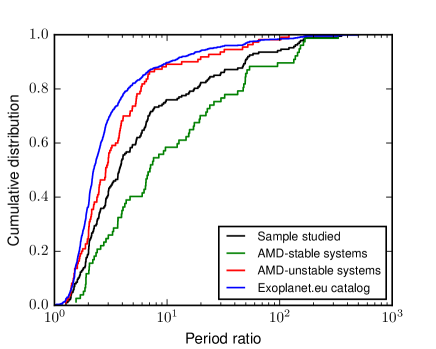
Figure 3: Cumulative distributions of the period ratios of adjacent planets in the sample studied here, of the AMD-stable systems (both weak and strong), AMD-unstable systems, and for all the systems referenced in the exoplanet.eu database.

We compare the cumulative distribution of the adjacent planets’ period ratios in our sample and that of all the multiplanetary systems in the database exoplanet.eu (see Fig. 3). The sample is biased toward higher period ratios. Indeed, most of the multiplanetary systems in the database come from the Kepler data. Since these systems are mostly tightly packed ones, their period ratios are rather small. However, the majority of them do not have measured eccentricities and are consequently excluded from this study. Our sample thus mostly contains systems detected by radial velocities (RV) methods that have, on average, higher period ratios.

Since all the AMD computations are done with the relative quantities $\alpha$ and $\gamma$, we can use equivalent quantities that are measured more precisely in observations than the masses and semi-major axis. We used the period ratios elevated to the power 3/2 instead of the semi-major axis ratios, and the minimum mass $m\sin(i)$ for RV system. This is not a problem for the computation of $\gamma$; if we assume that the systems are close to coplanarity, then

$$\gamma={{m}\over{m^{\prime}}}={{m\sin(i)}\over{m^{\prime}\sin(i)}}\simeq{{m\sin(i)}\over{m^{\prime}\sin(i^{\prime})}}\ .$$ (63)

Even though we assume the systems to be coplanar, we want to take into account the contribution of mutual inclinations to the AMD. Since we only have access to the eccentricities, we define the coplanar AMD of a system $C_{p}$, as the AMD of the same system if it was coplanar. We can also define

$$\beta_{p}=C_{p}/(\Lambda^{\prime}C_{c})\ ,$$ (64)

which is the coplanar AMD-stability coefficient. Motivated by both theoretical arguments on chaotic diffusion in the secular dynamics (Laskar, 1994, 2008) and observed correlations in statistical distributions (Xie et al., 2016), we assume that the AMD contribution of mutual inclinations is equal to that of the eccentricities. This hypothesis is equivalent to assuming the average equipartition of the AMD among the secular degrees of freedom for a chaotic system. The total AMD is thus twice the measured AMD, and in this study we use

$$\beta=2\beta_{p}\ .$$ (65)

We can also define a coplanar AMD-stability coefficient associated with the star, and similarly we set $\beta_{S}=2\beta_{Sp}$. We then compute the coefficients $\beta_{S}$ and $\beta$ for each pair and the associated uncertainty distributions. We list the results of the analysis in Table 3. In the considered dataset, 70 systems are AMD-stable. The majority of the highest multiplicity systems are AMD-unstable.

Table 3: Result of the analysis split in function of the multiplicity of the system

Multiplicity	Strong stable	Weak stable	Unstable	Total
2	42	21	34	97
3	4	1	17	22
4+	2	0	10	12
Total	48	22	61	131

In Figure 4 we plot the probability distribution of $\beta$ for the considered systems.

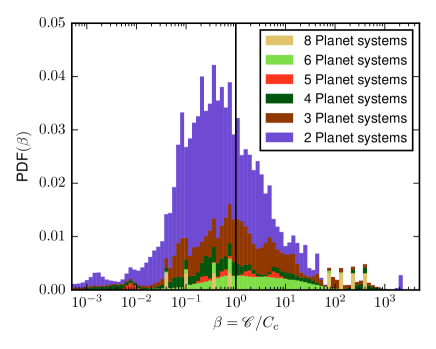
Figure 4: Probability distribution function of $\beta$ for the sample studied. The systems are grouped by multiplicity. The vertical line $\beta=1$ marks the separation between AMD-stable and AMD-unstable pairs.

5.2 Propagation of uncertainties

The uncertainties are propagated using Monte Carlo simulations of the distributions. After determining the distributions from the input quantities ($m,a,e$), we generate 10,000 values for each of these parameters. We then compute the derived quantities ($\alpha,\gamma,C_{c},\beta$…) in these 10,000 cases and the associated distributions.

For masses (or $m\sin(i)$ if no masses are provided) and periods, we assume a Gaussian uncertainty centred on the value referenced in the database and with standard deviation, the half width of the confidence interval. The distributions are truncated to 0.

For eccentricity distributions, the previous method does not provide satisfying results. Most of the Gaussian distributions constructed with the mean value and confidence interval given in the catalogue make negative eccentricities probable (in the case of almost circular planets with a large upper bound on the eccentricity). One solution is to assume that the rectangular eccentricity coordinates $(e\cos\omega,e\sin\omega)$ are Gaussian. Since the average value of $\omega$ has no importance in the computation of the eccentricity distribution, we assume it to be $0$. Therefore, $e\sin\omega$ has 0 mean. We define the distribution of $\tilde{e}=e\cos\omega$ as a Gaussian distribution with the mean value, the value referenced in the catalogue, and standard deviation, the half-width of the confidence interval. If we assume $e\sin\omega$ has the same standard deviation as $e\cos\omega$, we have $e\sin\omega=\tilde{e}-\langle\tilde{e}\rangle$. The distribution of $e$ is then deduced from that of $\tilde{e}$ using

$$e=\sqrt{{\tilde{e}}^{2}+(\tilde{e}-\langle\tilde{e}\rangle)^{2}}\ .$$ (66)

Using the Gaussian assumption means that some masses or periods can take values close to 0 with a small probability. This causes the distributions of $\alpha$ or $\gamma$ to diverge if it happens that $a^{\prime}$ or $m^{\prime}$ can take values close to 0. To address this issue, a linear expansion around the mean value is used for the quotients, for example for $\alpha$,

$$\alpha={{a}\over{a^{\prime}}}={{a}\over{\langle a^{\prime}\rangle}}\left(1-{{\Delta a^{\prime}}\over{\langle a^{\prime}\rangle}}\right)\ ,$$ (67)

with $\Delta a^{\prime}=a^{\prime}-\langle a^{\prime}\rangle$.

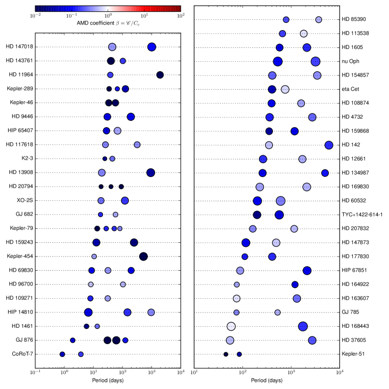
Figure 5: Architecture of the strong AMD-stable systems. Each planet is represented by a circle whose size is proportional to $\log_{10}(m),$ where $m$ is the mass of the planet. The colour represents the AMD-stability coefficient of the inner pair associated with the planet (in particular, the first planet is represented with the AMD-stability coefficient associated with the star $\beta_{S}$). This means that a red planet can collide with its inner neighbour

5.3 AMD-stable systems

As said above, we consider AMD-stable a system where collisions between planets are impossible because of the dynamics ruled by AMD ($\max\beta<1$). In addition, if the AMD-stability coefficient of the star $\beta_{S}<1$ (resp. $\beta_{S}>1$), the system is defined as strong AMD-stable (resp. weak AMD-stable).

5.3.1 Strong AMD-stable systems

The strong AMD-stable systems can be considered dynamically stable in the long term. In Figure 5, we plot the architecture of the strong AMD-stable systems. If the system is out of the mean motion resonance (MMR) islands, the AMD will not increase and therefore no collision between planets or with the star can occur. We can see in Figure 3 that the AMD-stable systems have period ratios on average larger than those from the sample.

5.3.2 Weak AMD-stable systems

As defined above, in a weak AMD-stable system, no planetary collisions can occur, but the innermost planet can increase its eccentricity up to 1 and collide with the star. We separate these systems from the strong AMD-stable ones because the system can still lose a planet only by AMD exchange. However, the remaining system will not be affected by the destruction of the inner planet. In Figure 6, we plot their architecture. In these systems, the inner planet is much closer to the star than the others.

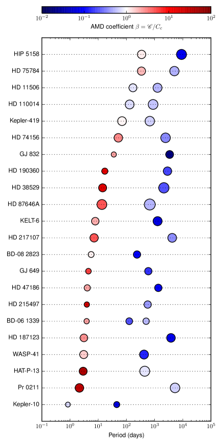
Figure 6: Architecture of the weak AMD-stable systems. Each planet is represented by a circle whose size is proportional to $\log_{10}(m),$ where $m$ is the mass of the planet. The colour represents the AMD-stability coefficient of the inner pair associated with the planet (in particular, the first planet is represented with the AMD-stability coefficient associated with the star $\beta_{S}$).

5.4 AMD-unstable systems

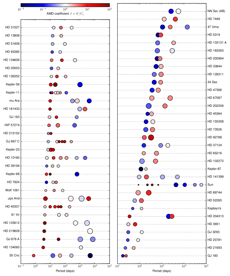
Figure 7: Architecture of the AMD-unstable systems. Each planet is represented by a circle whose size is proportional to $\log_{10}(m),$ where $m$ is the mass of the planet. The colour represents the AMD-stability coefficient of the inner pair associated with the planet (in particular, the first planet is represented with the AMD-stability coefficient associated with the star $\beta_{S}$).

The AMD-unstable systems have at least one unstable planet pair, but as we show in Figure 7 where we plot the architecture of these systems, this category is not homogeneous. It gathers high multiplicity systems where planets are too close to each other for the criterion to be valid, multiscale systems like the solar system where the inner system is AMD-unstable owing to its small mass in comparison to the outer part, systems experiencing mean motion resonances, etc. In all these cases, an in-depth dynamical study is necessary to determine the short- or long-term stability of these systems. In the following sections, we detail how the AMD-stability and AMD driven dynamics can help to understand these systems.

5.4.1 Hierarchically AMD-stable systems (solar system-like)

We first consider the solar system. Owing to the large amount of AMD created by the giant planets, the inner system is not AMD-stable (Laskar, 1997). However, long-term secular and direct integrations have shown that the inner system has a probability of becoming unstable of only 1% over 5 Gyr (Laskar, 2008; Laskar & Gastineau, 2009; Batygin et al., 2015). Indeed, the chaotic dynamics is mainly restricted to the inner system, while the outer system is mostly quasi-periodic. However, when AMD exchange occurs between the outer and inner systems, the inner system becomes highly unstable and can lose one or several planets.

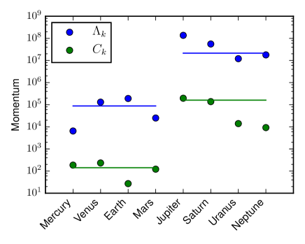
Figure 8: Circular momenta and AMD of the solar system planets. The horizontal lines correspond to the respective mean $\Lambda_{k}$ and $C_{k}$ for the inner and outer system.

In Figure 8 we plot the AMD and the circular momenta of the solar system planets. We see that the inner system planets (resp. the outer planets) have comparable AMD values. Laskar (2008) showed the absence of exchange between the two parts of the system. Moreover, the spacing of the planets follows surprisingly well the distribution laws mentioned in section 4 if we consider the two parts of the system separately (Laskar, 2000).

We see that given an analysis of the secular dynamics, the tools developed above can still help to understand how an a priori unstable system can still exist in its current state. The case of AMD-unstable systems with an AMD-stable part is not restricted to the solar system. If we look for systems where the outer part is AMD-stable while the whole system is AMD-unstable, we find four similar systems in our sample as shown in Figure 9. We call these systems hierarchic AMD-stable systems.

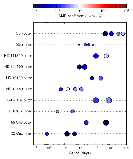
Figure 9: Examples of systems where the outer part is AMD-stable and the inner part becomes AMD-stable if considered alone.

5.4.2 Resonant systems

As shown by the cumulative distributions plotted in Figure 3, the AMD-unstable systems have period ratios that are lower than the AMD-stable systems. For example, in our sample 66% of the adjacent pairs of the AMD-unstable systems have a period ratio below 4, whereas this proportion is only 33% for the AMD-stable systems. For period ratios close to small integer ratios, the MMR can rule a great part of the dynamics. Particularly, if pairs of planets are trapped in a large resonance island, the system could be dynamically stable even if it is not AMD-stable.

Individual dynamical studies are necessary in order to claim that a system is stable due to a MMR. We note, however, that the AMD-unstable systems considered here are statistically constituted of more resonant pairs than a typical sample in the catalogue.

5.4.3 Concentration around MMR

Here we want to test whether the unstable systems have been drawn randomly from the exoplanet.eu catalogue or if the period ratios of the pairs of adjacent planets are statistically closer to small integer ratios. We denote $\mathcal{H}_{0}$, the hypothesis that the period ratios of the unstable systems have been drawn randomly from the catalogue distribution. We consider only the period ratios lower than 4 because the higher ones are not significant for a study of the MMR. We plot in figure 10 the cumulative distribution of the period ratios of the AMD-unstable systems, as well as the cumulative distribution of the period ratios of all the systems of exoplanet.eu. We call $R_{u}$ the set of period ratios of the AMD-unstable planets.

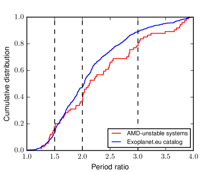
Figure 10: Cumulative period ratios of the AMD-unstable systems and of all systems in the catalogue. The vertical line represents low order MMR.

We first test $\mathcal{H}_{0}$ via a Kolmogorov-Smirnov test (Lehmann & Romano, 2006) between the sample $R_{u}$ and the period ratios of the catalogue. The test fails to reject $\mathcal{H}_{0}$ with a p-value of about 9%. Therefore, we cannot reject $\mathcal{H}_{0}$ on the global shape of the distribution of the AMD-unstable period ratios.

However, we want to determine if the AMD-unstable pairs are close to small integer ratios, which means studying the fine structure of the distribution. We propose here another method for demonstrating this.

Let us denote the probability density of the catalogue period ratios $f$ and the associated cumulative distribution $\mathcal{F}$. Let us consider an interval $I_{x}=(x,x+\Delta x)$, if we assume $\mathcal{H}_{0}$, the probability for a ratio $r$ to be in $I_{x}$ is

$$\mathcal{P}(r\in I_{x}|\mathcal{H}_{0}) = \int_{x}^{x+\Delta x}f(r^{\prime})\mathrm{d}r^{\prime}$$ (68)

$$= \mathcal{F}(x+\Delta x)-\mathcal{F}(x)=\Delta\mathcal{F}(x)\ .$$

Therefore, the probability that more than $k_{0}$ pairs out of $N$ pairs drawn randomly from the distribution $\mathcal{F}$ are in $I_{x}$ is

$$\mathcal{P}(x,k_{0}|\mathcal{H}_{0})=\sum_{k=k_{0}}^{N}\binom{N}{k}(1-\Delta\mathcal{F})^{N-k}\Delta\mathcal{F}^{k}.$$ (69)

This is the probability of a binomial trial. From now on, $N$ designates the number of period ratios in $R_{u}$.

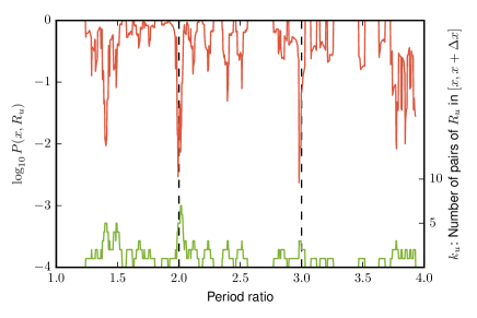
Figure 11: Red curve: Probability of observing more than $k_{0}$ pairs in the interval $I_{x}$ given a probability density $f$. Green curve: $k_{0}$ is the number of pairs in $I_{x}$ for the unstable systems $R_{u}$

For a given $\Delta x$, we can compute the probability $P(x,R_{u})=\mathcal{P}(x,k_{u}(x))$, where $k_{u}(x)$ is the number of pairs from $R_{u}$ in $I_{x}$. This probability measures the likelihood of a concentration of elements of $R_{u}$ around $x$, assuming they were drawn from $\mathcal{F}$. We choose $\Delta x=0.05$ and plot the function $P(x,R_{u})$ as well as $k_{u}$ in Figure 11. We observe that the concentrations around 3 and 2 are very unlikely with a probability of $2.3\times 10^{-3}$ and $2.9\times 10^{-3}$, respectively. Other peaks appear for $x=1.4$ and around 3.8. However, $P(x,R_{u})$ is the probability of seeing a concentration around $x$ precisely. It is not the probability of observing a concentration somewhere between 1 and 4.

To demonstrate that the concentrations around 2 and 3 are meaningful, we compare this result to samples drawn randomly from the distribution $\mathcal{F}$. We create 10,000 datasets $R_{\alpha}$ by drawing $N$ points from $\mathcal{F}$ and compute $P(x,R_{\alpha})$ for these datasets. Then, we record the two minimum values (at least distant by more than $\Delta x$) and plot the distribution of these minima on Figure 12. From these simulations, we see that on average 17.2% of the samples have a minimum as small as $R_{u}$. However, the presence of a secondary peak as significant as the second one of $R_{u}$ has a probability of 1.3%. Moreover, the $R_{u}$ concentrations are clearly situated around low integer ratios, which would not be the case in general for a randomly generated sample.

We thus demonstrated here that the AMD-unstable systems period ratios are significantly concentrated around low integer ratios. While we do not prove that the pairs of planets close to these ratios are actually in MMR, this result further motivates investigations toward the behaviour of these pairs in a context of secular chaotic dynamics.

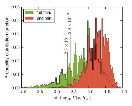
Figure 12: Probability density function of the two first minimum values of $P(x,R_{\alpha})$ from 10,000 samples $R_{\alpha}$ drawn from the $\mathcal{F}$ distribution.

6 Conclusion

The angular momentum deficit (AMD) (Laskar, 1997, 2000) is a key parameter for the understanding of the outcome of the formation processes of planetary systems (e.g. Chambers, 2001; Morbidelli et al., 2012; Tremaine, 2015). We have shown here how AMD can be used to derive a well-defined stability criterion: the AMD-stability. The AMD-stability of a system can be checked by the computation of the critical AMD $C_{c}$ (eq. 39) and AMD-stability coefficients $\beta_{i}$ that depend only on the eccentricities and ratios of semi-major axes and masses (Eqs. 33, 39, 43, 62). This criterion thus does not depend on the degeneracy of the masses coming from radial velocity measures. Moreover, the uncertainty on the relative inclinations can be compensated by assuming equipartition of the AMD between eccentricities and inclinations.

AMD-stability will ensure that in the absence of mean motion resonances, the system is long-term stable. A rapid estimate of the stability of a system can thus be obtain by a short-term integration and the simple computation of the AMD-stability coefficients.

We have also proposed here a classification of the planetary systems based on AMD-stability (Section 5). The strong AMD-stable systems are the systems where no planetary collisions are possible, and no collisions of the inner planet with its central star, while the weak AMD-stable systems allow for the collision of the inner planet with the central star. The AMD-unstable systems are the systems for which the AMD-coefficient does not prevent the possibility of collisions. The solar system is AMD-unstable, but it belongs to the subcategory of hierarchical AMD-stable systems that are AMD-unstable but become AMD-stable when they are split into two parts (giant planets and terrestrial planets for the solar system) (Laskar, 2000). Out of the 131 studied systems from exoplanet.eu, we find 48 strong AMD-stable, 22 weak AMD-stable, and 61 AMD-unstable systems, including 5 hierarchical AMD-stable systems.

As for the solar system, the AMD-unstable systems are not necessarily unstable, but determining their stability requires some further dynamical analysis. Several mechanisms can stabilise AMD-unstable systems. The absence of secular chaotic interactions between parts of the systems, like in the solar system case, or the presence of mean motion resonances, protecting pairs of planets from collision. In this case, the AMD-stability classification is still useful in order to select the systems that require this more in-depth dynamical analysis. It should also be noted that the discovery of additional planets in a system will require a revision of the computation of the AMD-stability of the system. This additional planet will always increase the total AMD, and thus the maximum AMD-coefficient of the system, decreasing its AMD-stability unless it is split into two subsystems.

In the present work, we have not taken into account mean motion resonances (MMR) and the chaotic behaviour resulting from their overlap. We aim to take these MMR into consideration in a forthcoming work. Indeed, the criterion regarding MMR developed by Wisdom (1980) or more recently Deck et al. (2013) may help to improve our stability criterion by considering the MMR chaotic zone as a limit for stability instead of the limit considered here that is given by the collisions of the orbits (Eqs. 39). The drawback will then most probably be giving up the rigorous results that we have established in section 3, and allowing for additional empirical studies. The present work will in any case remain the backbone of these further studies. Note: The AMD-stability coefficients of selected planetary systems will be made available on the exoplanet.eu database.

Appendix A Intersection of planar orbits

In this section, we present an efficient algorithm for the computation of the intersection of two elliptical orbits in the plane, following (Albouy 2002). Let us consider an elliptical orbit defined by $(\mu,{\bf r},{\bf\dot{r}})$ and let ${\bf G}={\bf r}\wedge{\bf\dot{r}}$ be the angular momentum per unit of mass. The Laplace vector

$${\bf P}={{\displaystyle{\bf\dot{r}}\wedge{\bf G}}\over{\displaystyle\mu}}-{{\displaystyle{\bf r}}\over{\displaystyle r}}$$ (70)

is an integral of the motion with coordinates $(e\cos\omega,e\sin\omega)$. One has

$${\bf P}\cdot{\bf r}={{G^{2}}\over{\mu}}-r=p-r,$$ (71)

where $p=a(1-e^{2})$ is the parameter of the ellipse. Let ${\bf r}=(x,y)$ in the plane. We can consider the ellipse in three-dimensional space $(x,y,r)$ as the intersection of the cone

$$r^{2}=x^{2}+y^{2}$$ (72)

with the plane defined by Eq. (71), that is

$$x(e\cos\omega)+y(e\sin\omega)+r=p$$ (73)

If we consider now two orbits ${\cal O}_{1}$ and ${\cal O}_{2}$. Their intersection is easily obtained as the intersection of the line of intersection of the two planes

$${\displaystyle x(e_{1}\cos\omega_{1})+y(e_{1}\sin\omega_{1})+r=p_{1}} {\displaystyle x(e_{2}\cos\omega_{2})+y(e_{2}\sin\omega_{2})+r=p_{2}}$$ (74)

with the cone of equation $r^{2}=x^{2}+y^{2}$. Depending on the initial conditions, if ${\cal O}_{1}$ and ${\cal O}_{2}$ are distinct, we will get either 0, 1, or 2 solutions.

Figure 13: Elliptical orbit, as the intersection of the cone $r^{2}=x^{2}+y^{2}$ and the plane ${\bf P}\cdot{\bf r}+r=p$ .

Appendix B AMD in the averaged equations

In this section we show that the AMD conserves the same form in the averaged planetary Hamiltonian at all orders. More generally, this is true for any integral of $H$ which does not depend on the longitude $\lambda_{k}$. Let

$$H=H_{0}(\Lambda)+\varepsilon H_{1}(\Lambda,\lambda,J,\phi)$$ (75)

be a perturbed Hamiltonian system, and let $K(\Lambda,J,\phi)$ be a first integral of $H(\Lambda,\lambda,J,\phi)$ (such that $\{K,H\}=0$, where $\{\cdot,\cdot\}$ is the usual Poisson bracket), and independent of $\lambda$. In addition, let

$$H^{\prime}={\rm e}^{L_{S}}H$$ (76)

be a formal averaging of $H$ with respect to $\lambda$. If $S(\Lambda,\lambda,J,\phi)$ is a generator defined as below (Eqs. 78, 80, 81), such that $H^{\prime}$ is independent of $\lambda$. Then, $K$ is an integral of $H^{\prime}$, i.e.

$$\{K,H^{\prime}\}=0$$ (77)

The generator $S=\varepsilon S_{1}+\varepsilon^{2}S_{2}+\varepsilon^{3}S_{3}+\cdots$ is obtained formally through the identification order by order

$${\displaystyle H^{\prime}_{0}=H_{0}} {\displaystyle H^{\prime}_{1}=H_{1}+} {\displaystyle\{H_{0},S_{1}\}} {\displaystyle H^{\prime}_{2}=} {\displaystyle\{H_{0},S_{2}\}+{{\displaystyle 1}\over{\displaystyle 2}}\{\{H_{0},S_{1}\},S_{1}\}+\{H_{1},S_{1}\}} {\displaystyle\dots}$$ (78)

For any function $G(\Lambda,\lambda,J,\phi)$, let

$${\langle G\rangle_{\bm{\lambda}}={{1}\over{(2\pi)^{m}}}}\int G\mathrm{d}^{m}\bm{\lambda}$$ (79)

be the average of $G$ over all the angles $\lambda_{k}$. For each $n\geq 1$, the $S_{n}$ is obtained through the resolution of an equation of the form

$$H^{\prime}_{n}=\{H_{0},S_{n}\}+{\cal R}_{n},$$ (80)

where ${\cal R}_{n}$ belongs to ${\cal L}(H_{0},H_{1},S_{1},\dots,S_{n-1})$, the Lie algebra generated by $(H_{0},H_{1},S_{1},\dots,S_{n-1})$. $H^{\prime}_{n}$ will be the averaged part of ${\cal R}_{n}$, $\langle{\cal R}_{n}\rangle_{\lambda}$, and $S_{n}$ is obtained by solving the homological equation

$$\{H_{0},S_{n}\}=\langle{\cal R}_{n}\rangle_{\bm{\lambda}}-{\cal R}_{n}\ .$$ (81)

We show by recurrence that $\{K,S_{n}\}=0$ for all $n\geq 1$. First, we note that as $\{K,H_{0}\}=0$, we also have $\{K,H_{1}\}=0$. As $K$ is independent of $\lambda_{k}$, we also have for all $G$

$$\langle\{K,G\}\rangle_{\lambda}=\{K,\langle G\rangle_{\lambda}\}$$ (82)

This can be seen by formal expansion of $G$ in a Fourier series $G=\sum g_{k}{\rm e}^{i\langle k,\lambda\rangle}$. We have thus $\langle G\rangle_{\lambda}=g_{0}$. Let us assume now that $\{K,S_{k}\}=0$ for all $k\leq n$. As ${\cal R}_{n+1}\in{\cal L}(H_{0},H_{1},S_{1},\dots,S_{n})$, we also have $\{K,{\cal R}_{n+1}\}=0$, and from (82) $\{K,\langle{\cal R}_{n+1}\rangle_{\lambda}\}=0$ and thus

$$\{K,\{H_{0},S_{n+1}\}\}=0$$ (83)

Using the Jacobi identity, as $\{F,H_{0}\}=0$, we have

$$\{H_{0},\{K,S_{n+1}\}\}=0$$ (84)

The solution of the homological equation (81) is unique up to a term independent of $\lambda$. But as ${\langle\{K,S_{n+1}\}\rangle_{\lambda}=0}$, then the only possible solution for (84) is

$$\{K,S_{n+1}\}=0\ .$$ (85)

In the same way, as $H^{\prime}_{1}=\langle H_{1}\rangle_{\lambda}$, we have $\{K,H_{1}^{\prime}\}=\langle\{K,H_{1}\}\rangle_{\lambda}=0$. Thus $\{K,\{H_{0},S_{1}\}\}=0$, by the Jacobi identity, $\{H_{0},\{K,S_{1}\}\}=0$, and as previously, $\{K,S_{1}\}=0$. Our recurrence is thus complete and it follows immediately that $\{K,H^{\prime}\}=0$.

Appendix C Special values of $C_{c}(\alpha,\gamma)$

This appendix provides the detailed computations and proofs of the results of section 3.2

C.1 Asymptotic value of $C_{c}(\alpha,\gamma)$ for $\gamma\rightarrow 0$

We have shown that $e_{c}(\alpha,\gamma)$ is a differentiable function of $\gamma$, which is monotonic (45) and bounded ($e_{c}(a,\gamma)\in[0,1]$). The limit $e_{c}(\alpha,0)=\raisebox{2.15277pt}{\scalebox{0.8}{$\displaystyle\lim_{\gamma\rightarrow 0}\;$}}e_{c}(\alpha,\gamma)$ exists for all $\alpha\in]0,1]$. If $e_{c}(\alpha,\gamma)$ is a solution of equation(39), it will also be a solution of the following cubic equation (in $e$), which is directly obtained from (39) by squaring, multiplication, and simplification by $\alpha(1+e):$

$${\displaystyle K(e,\alpha,\gamma)=\alpha(\gamma^{2}-\alpha)e^{3}} {\displaystyle-(2-\alpha)(\gamma^{2}-\alpha)e^{2}} {\displaystyle-(1-\alpha^{2})e+(1-\alpha)^{2}=0}$$ (86)

As $e_{c}(\alpha,\gamma)$, is a continuous function of $\gamma$, when $\gamma\rightarrow 0$ the limits $e_{0c}(\alpha)$ will satisfy the limit equation

$$K_{0}(e,\alpha)=(1-\alpha-\alpha e)^{2}(1-e)=0$$ (87)

with solutions $e_{0}=1/\alpha-1$ and $e_{1}=1$. Depending on $\alpha$, several cases are treated:

$\bm{\alpha<1/2}$ :

We have then $e_{0}>1$, and the only possibility for $e_{c}(\alpha,0)$ is $e_{1}=1$; as it is the only root of (87) which belongs to $[0,1],$ we have thus

$$\lim_{\gamma\rightarrow 0}e_{c}(\alpha,\gamma)=1$$ (88)

We have then

$$\lim_{\gamma\rightarrow 0}e_{c}^{\prime}(\alpha,\gamma) = 1-2\alpha\ ;$$

$$\lim_{\gamma\rightarrow 0}C_{c}(\alpha,\gamma) = 1-2\sqrt{\alpha(1-\alpha)}\ ;$$ (89)

In order to study the behaviour of $e_{c}(\alpha,\gamma)$ in the vicinity of $\gamma=0$, we can differentiate $K(e_{c}(\alpha,\gamma),\gamma)=0$ twice, which gives

$${{\displaystyle de_{c}}\over{\displaystyle d\gamma}}(\alpha,0)=0\,;\qquad{{\displaystyle d^{2}e_{c}}\over{\displaystyle d\gamma^{2}}}(\alpha,0)={{\displaystyle 4(\alpha-1)}\over{\displaystyle(1-2\alpha)^{2}}}<0\ ,$$ (90)

thus $e_{c}(\alpha,\gamma)$ decreases with respect to $\gamma$ at $\gamma=0$.

The second order development of $C_{c}$ gives

$$C_{c}(\alpha,\gamma)=1-2\sqrt{\alpha(1-a)}+\gamma\sqrt{\alpha}-\gamma^{2}\sqrt{{{1}\over{\alpha}}-1}+\mathrm{O}(\gamma^{3}).$$ (91)

$\bm{\alpha>1/2}$ :

In this case, $e_{0}<1$. As $e_{c}(\alpha,\gamma)\in]0,e_{0}[$, we have $e_{c}(\alpha,0)\in[0,e_{0}]$, which gives as the unique possibility

$$\lim_{\gamma\rightarrow 0}e_{c}(\alpha,\gamma)=e_{0}$$ (92)

with

$$\lim_{\gamma\rightarrow 0}e_{c}^{\prime}(\alpha,\gamma)=0\ ;\qquad\lim_{\gamma\rightarrow 0}C_{c}(\alpha,\gamma)=0\ .$$ (93)

By setting $\gamma=0$ in (45), we also obtain

$${{\displaystyle de_{c}}\over{\displaystyle d\gamma}}(\alpha,0)=-{{\displaystyle e_{0}}\over{\displaystyle\alpha^{3/2}\sqrt{1-e_{0}^{2}}}}<0\ .$$ (94)

The development of $C_{c}$ gives

$$C_{c}(\alpha,\gamma)=\gamma\left(\sqrt{\alpha}-\sqrt{2-{{1}\over{\alpha}}}\right)-{{\displaystyle\gamma^{2}}\over{\displaystyle 2\alpha-1}}{{\displaystyle(1-\alpha)^{2}}\over{\displaystyle\alpha}}+\mathrm{O}(\gamma^{3}).$$ (95)

$\bm{\alpha=1/2}$ :

In this case, $e_{0}=1$, and the only solution is

$$\lim_{\gamma\rightarrow 0}e_{c}(\alpha,\gamma)=1$$ (96)

and

$$\lim_{\gamma\rightarrow 0}e_{c}^{\prime}(\alpha,\gamma)=0\ ;\qquad\lim_{\gamma\rightarrow 0}C_{c}(\alpha,\gamma)=0\ .$$ (97)

Moreover, equation (86) becomes $\gamma^{2}2e^{2}(3-e)=(1-e)^{3}$. We obtain thus the asymptotic value for $e_{c}(1/2,\gamma)$ when $\gamma\rightarrow 0$ as

$$1-e_{c}({{1}\over{2}},\gamma)\,\,{\sim}\,\,(4\gamma)^{2/3}.$$ (98)

For $\alpha=1/2$, the development of $C_{c}$ in $\gamma$ contains non-polynomial terms in $\gamma$ giving

$$C_{c}(1/2,\gamma)={{\gamma}\over{\sqrt{2}}}-2^{-1/3}\gamma^{4/3}-2^{-4/3}\gamma^{2}+\mathrm{O}(\gamma^{8/3})$$ (99)

C.2 Asymptotic value of $C_{c}(\alpha,\gamma)$ for $\gamma\rightarrow+\infty$

This case is more simple. If $e_{c}(\alpha,\gamma)$ is a solution of Eq. (39), then it will also be a solution of eq. (86), and thus of

$${{\displaystyle K(e,\alpha,\gamma)}\over{\displaystyle\gamma^{2}}}=0$$ (100)

As $e_{c}(\alpha,\gamma)$ is monotonic and bounded, it has a limit when $\gamma\rightarrow+\infty$, which will verify the limit equation (100), when $\gamma\rightarrow+\infty$, that is

$$K_{\infty}(\alpha,e)=e^{2}(2-\alpha-\alpha e)=0$$ (101)

As $0<\alpha<1$, the only solution is $e=0$, and thus

$$\lim_{\gamma\rightarrow+\infty}e_{c}(\alpha,\gamma)=0$$ (102)

and

$$\lim_{\gamma\rightarrow+\infty}e_{c}^{\prime}(\alpha,\gamma)=1-\alpha\ ;\quad\lim_{\gamma\rightarrow+\infty}C_{c}(\alpha,\gamma)=1-\sqrt{\alpha(2-\alpha)}\$$ (103)

and more precisely

$${\displaystyle C(\alpha,\gamma)=1} {\displaystyle-\sqrt{\alpha(2-\alpha)}-{{\displaystyle 1}\over{\displaystyle 2\gamma}}{{\displaystyle\sqrt{\alpha}(1-\alpha)^{2}}\over{\displaystyle 2-\alpha}}} {\displaystyle+{{\displaystyle 1}\over{\displaystyle\gamma^{2}}}{{\displaystyle\sqrt{\alpha(2-\alpha)}(1-\alpha)^{2}}\over{\displaystyle 2(2-\alpha)^{3}}}+\mathrm{O}\left({{\displaystyle 1}\over{\displaystyle\gamma^{3}}}\right)}$$ (104)

C.3 Study of $C_{c}(\alpha,\gamma)$ for $\gamma=1$ and $\gamma=\sqrt{\alpha}$.

For $\gamma=1$ or $\gamma=\sqrt{\alpha}$, we can also obtain simple expressions for $C_{c}(\alpha,\gamma)$. Indeed, If $\gamma=1$, $K(e,\alpha,\gamma)$ factorises in $(1-\alpha)(1+e)(\alpha e^{2}-2e+1-\alpha)$ and we have a single solution for $e_{c}$ in the interval $[0,1]$,

$${\displaystyle e_{c}(\alpha,1)} {\displaystyle={{\displaystyle 1-\sqrt{1-\alpha+\alpha^{2}}}\over{\displaystyle\alpha}}\ ;} {\displaystyle e_{c}^{\prime}(\alpha,1)} {\displaystyle=\sqrt{1-\alpha+\alpha^{2}}-\alpha\ ;}$$ (105)

and

$${\displaystyle C_{c}(\alpha,1)=} {\displaystyle\sqrt{\alpha}-{{\displaystyle\sqrt{\alpha-2+2\sqrt{1-\alpha+\alpha^{2}}}}\over{\displaystyle\sqrt{\alpha}}}} {\displaystyle+1-\sqrt{\alpha}\sqrt{1-2\alpha+2\sqrt{1-\alpha+\alpha^{2}}}}$$ (106)

For $\gamma=\sqrt{\alpha}$, the cubic equation (86) reduces to

$$K(\alpha,\sqrt{\alpha})=-(1-\alpha^{2})e+(1-\alpha)^{2}=0$$ (107)

with the single solution

$$e_{c}(\alpha,\sqrt{\alpha})=e_{c}^{\prime}(\alpha,\sqrt{\alpha}))={{\displaystyle 1-\alpha}\over{\displaystyle 1+\alpha}}$$ (108)

and

$$C_{c}(\alpha,\sqrt{\alpha})=(1-\sqrt{\alpha})^{2}$$ (109)

C.4 $C_{c}(\alpha,\gamma)$ for $\alpha\longrightarrow 1$

Let us denote $\eta=1-\alpha$. The equation 86 can be developed in $\eta$,

$$K(e,\alpha,\gamma) = (\gamma^{2}-1)e^{2}(e-1)+$$ (110)

$$= \eta e\left((\gamma^{2}-1)(e-e^{2})-2\right)+$$

$$= \eta^{2}(1-e-e^{2}-e^{3})=0.$$

The zeroth and first orders of equation 110 imply that $e_{c}$ must go to zero; moreover, it scales with $\eta$. We write $e_{c}(\eta,\gamma)=\kappa(\gamma)\eta+\mathrm{o}(\eta)$. We inject this expression in 110 and keep the second order in $\eta$

$$(\gamma^{2}-1)\kappa^{2}+2\kappa-1=0.$$ (111)

We keep the solution that is positive and continuous in $\gamma$ and we have

$$e_{c}(\eta,\gamma)={{\displaystyle\eta}\over{\displaystyle\gamma+1}}+\mathrm{o}(\eta).$$ (112)

If we now compute $C_{c}$ developed for $\alpha\longrightarrow 1$ we have

$$C_{c}(1-\eta,\gamma) = k(\gamma)\eta^{2}+\mathrm{o}(\eta^{2})$$ (113)

$$= {{\displaystyle 1}\over{\displaystyle 2}}{{\displaystyle\gamma}\over{\displaystyle\gamma+1}}\eta^{2}+\mathrm{o}(\eta^{2})$$

References

- Albouy (2002) Albouy, A. 2002, Lectures on the two-body problem (Princeton University Press)
- Batygin et al. (2015) Batygin, K., Morbidelli, A., & Holman, M. J. 2015, The Astrophysical Journal, 799, 120
- Chambers (2001) Chambers, J. 2001, Icarus, 152, 205
- Chambers (2013) Chambers, J. 2013, Icarus, 224, 43
- Chambers et al. (1996) Chambers, J., Wetherill, G., & Boss, A. 1996, Icarus, 119, 261
- Deck et al. (2013) Deck, K. M., Payne, M., & Holman, M. J. 2013, The Astrophysical Journal, 774, 129
- Fabrycky et al. (2014) Fabrycky, D. C., Lissauer, J. J., Ragozzine, D., et al. 2014, The Astrophysical Journal, 790, 146
- Fang & Margot (2012) Fang, J. & Margot, J.-L. 2012, The Astrophysical Journal, 761, 92
- Fang & Margot (2013) Fang, J. & Margot, J.-L. 2013, The Astrophysical Journal, 767, 115
- Figueira et al. (2012) Figueira, P., Marmier, M., Boué, G., et al. 2012, Astronomy & Astrophysics, 541, A139
- Gladman (1993) Gladman, B. 1993, Icarus, 106, 247
- Graner & Dubrulle (1994) Graner, F. & Dubrulle, B. 1994, Astronomy and Astrophysics, 282, 262
- Hernández-Mena & Benet (2011) Hernández-Mena, C. & Benet, L. 2011, Monthly Notices of the Royal Astronomical Society, 412, 95
- Kokubo & Genda (2010) Kokubo, E. & Genda, H. 2010, The Astrophysical Journal, 714, L21
- Laskar (1994) Laskar, J. 1994, Astronomy and Astrophysics, 287, L9
- Laskar (1997) Laskar, J. 1997, Astronomy and Astrophysics, 317, L75
- Laskar (2000) Laskar, J. 2000, Physical Review Letters, 84, 3240
- Laskar (2008) Laskar, J. 2008, Icarus, 196, 1
- Laskar & Gastineau (2009) Laskar, J. & Gastineau, M. 2009, Nature, 459, 817
- Laskar & Robutel (1995) Laskar, J. & Robutel, P. 1995, Celestial Mechanics & Dynamical Astronomy, 62, 193
- Lehmann & Romano (2006) Lehmann, E. L. & Romano, J. P. 2006, Testing statistical hypotheses (Springer Science & Business Media)
- Lissauer et al. (2011) Lissauer, J. J., Ragozzine, D., Fabrycky, D. C., et al. 2011, The Astrophysical Journal Supplement Series, 197, 8
- Marchal & Bozis (1982) Marchal, C. & Bozis, G. 1982, Celestial Mechanics, 26, 311
- Mayor et al. (2011) Mayor, M., Marmier, M., Lovis, C., et al. 2011, eprint arXiv:1109.2497
- Moorhead et al. (2011) Moorhead, A. V., Ford, E. B., Morehead, R. C., et al. 2011, The Astrophysical Journal Supplement Series, 197, 1
- Morbidelli et al. (2012) Morbidelli, A., Lunine, J., O’Brien, D., Raymond, S., & Walsh, K. 2012, Annual Review of Earth and Planetary Sciences, 40, 251
- Nieto (1972) Nieto, M. M. 1972, The Titius-Bode law of planetary distances: its history and theory (Pergamon Press), 161
- Poincaré (1905) Poincaré, H. 1905, Leçons de mécanique céleste, Tome I (Gauthier-Villars. Paris)
- Pu & Wu (2015) Pu, B. & Wu, Y. 2015, The Astrophysical Journal, 807, 44
- Ramos et al. (2015) Ramos, X. S., Correa-Otto, J. A., & Beaugé, C. 2015, Celestial Mechanics and Dynamical Astronomy, 123, 453
- Raymond et al. (2006) Raymond, S. N., Quinn, T., & Lunine, J. I. 2006, Icarus, 183, 265
- Schneider et al. (2011) Schneider, J., Dedieu, C., Le Sidaner, P., Savalle, R., & Zolotukhin, I. 2011, Astronomy & Astrophysics, 532, A79
- Shabram et al. (2016) Shabram, M., Demory, B.-O., Cisewski, J., Ford, E. B., & Rogers, L. 2016, The Astrophysical Journal, 820, 93
- Smith & Lissauer (2009) Smith, A. W. & Lissauer, J. J. 2009, Icarus, 201, 381
- Tremaine (2015) Tremaine, S. 2015, The Astrophysical Journal, 807, 157
- Weidenschilling (1977) Weidenschilling, S. J. 1977, Astrophysics and Space Science, 51, 153
- Winn & Fabrycky (2015) Winn, J. N. & Fabrycky, D. C. 2015, Annual Review of Astronomy and Astrophysics, 53, 409
- Wisdom (1980) Wisdom, J. 1980, The Astronomical Journal, 85, 1122
- Wright et al. (2011) Wright, J. T., Fakhouri, O., Marcy, G. W., et al. 2011, Publications of the Astronomical Society of the Pacific, 123, 412
- Xie et al. (2016) Xie, J.-W., Dong, S., Zhu, Z., et al. 2016, Proceedings of the National Academy of Sciences, 113, 11431