Longitudinal $W$ boson scattering in a light scalar top scenario

Abstract

Scalar tops in the supersymmetric model affect the potential of the standard model-like Higgs at the quatum level. In light of the equivalence theorem, the deviation of the potential from the standard model can be traced by longitudinal gauge bosons. In this work, high energy longitudinal $W$ boson scattering is studied in a TeV-scale scalar top scenario. ${\cal O}$(1–10%) deviation from the standard model prediction in the differential cross section is found depending on whether the observed Higgs mass is explained only by scalar tops or by additional contributions at a higher scale.

I Introduction

The recent discovery of the Higgs boson confirmed the standard model (SM) of particle physics Aad:2012tfa ; Chatrchyan:2012xdj . Since then Higgs properties have been measured at the LHC and found to be consistent with the standard model prediction Higg_ATLAS&CMS ; besides, there has been no sign beyond the standard model in the experiment. It is widely believed, however, that the standard model is not the ultimate theory. Superstring theory is one of candidates for the “theory of everything”. It requires supersymmetry (SUSY) due to consistency, which gives rise to lots of phenomenological consequences beyond the standard model. For example, it provides a candidate for dark matter, and three gauge coupling constants are unified at the grand unification scale. Supersymmetry affects the Higgs sector too. In SUSY another Higgs doublet must be introduced for phenomenologically acceptable Higgs mechanism to work. In the supersymmetric Higgs sector, the electroweak symmetry breaking (EWSB) is induced by renormalization flow of parameters in the Higgs sector, which is a solution to the origin of the EWSB since in the SM it is induced by the ad hoc tachyonic Higgs mass term. In spite of such a drastic extension, the Higgs sector in the supersymmetric model reduces to the one in the SM below the electroweak scale when superpartners are much heavier than the electroweak scale. Considering the current status, i.e., no sign of a new particle so far, this might be the case, and then it might be difficult to observe a clue of supersymmetry even in future collider experiments.

In such a circumstance, it is worth recalling that the observed 125 GeV Higgs mass cannot be explained in SUSY at tree level. It is explained by scalar top (“stop”) loop contribution, for example, in the minimal supersymmetric standard model (MSSM) Haber:1990aw ; Ellis:1990nz ; Ellis:1991zd ; Okada:1990vk ; Okada:1990gg ; Brignole:1992uf . This fact indicates that stop has an impact on the SM Higgs potential at the quantum level, which is similar to the Higgs sector in classical scale invariant model. In a simple classical scale invariant model (a) SM singlet scalar(s) is (are) introduced. They affect the Higgs potential at quantum level, which induces the EWSB radiatively. In this framework, the singlet loop determines the curvature of the Higgs potential around the minimum, i.e., the Higgs mass. Although Higgs properties, such as mass, production and decay rates at collider experiments, are almost consistent with the SM values, the Higgs self-couplings are predicted to significantly deviate from the SM ones Dermisek:2013pta ; Endo:2015ifa ; Hashino:2015nxa . This means that Higgs potential is the same locally around the minimum but not in a global picture. Such an effect is imprinted in ficticious bosons in the Higgs doublet, which are absorbed into longitudinal polarization of the gauge bosons. While the measurement of the Higgs self-couplings is one of main goals of the next-generation lepton collider, e.g., the International Linear Collider (ILC), the deviation from the SM in the Higgs sector can be also probed at the LHC in the gauge boson scattering process. It is pointed out in Ref. Endo:2016koi that the differential cross sections of longitudinal gauge boson scattering processes $W^{+}_{L}W^{+}_{L}\to W^{+}_{L}W^{+}_{L}$ and $W^{+}_{L}W^{-}_{L}\to W^{+}_{L}W^{-}_{L}$ are changed by more than ${\cal O}$(10%) in the model, which is described by off-shell Higgs. Namely the discrepancy between the classical scale invariant model and the SM can be found in off-shell Higgs in the propagator, for which the longitudinal gauge boson scattering a good probe.

In supersymmetric model, stops are expected to play a role similar to the singlet scalars. In this paper we analyze the longitudinal gauge boson scattering in the framework of the supersymmetric model. Following the analysis in Ref. Endo:2016koi , we formulate the leading order amplitudes of the processes and discuss the deviation from the standard model prediction numerically.

In the study we consider stops with a mass of less than a few TeV. Such light stop scenario is motivated by naturalness argument, and part of parameter space of the scenario has already been excluded by the direct search at the LHC. In Ref. Aad:2015pfx scalar top pair production is analyzed in both a simplified model and phenomenologically tempered SUSY models in conserved R-parity using Run 1 data. The updated studies at $\sqrt{s}=13$ TeV  ATLAS:2016jaa ; Aaboud:2016tnv ; CMS:2016mwj ; Khachatryan:2016oia have shown that lighter stop mass region $m_{\tilde{t}_{1}}\lesssim 850~{}{\rm GeV}$ is excluded at 95%CL when the lightest neutralino mass $m_{\tilde{\chi}_{1}^{0}}$ is less than about 300 GeV. On the other hand, $m_{\tilde{t}_{1}}\gtrsim 400~{}{\rm GeV}$ and $m_{\tilde{\chi}_{1}^{0}}\gtrsim 300~{}{\rm GeV}$ (with $m_{\tilde{t}_{1}}>m_{\tilde{\chi}_{1}^{0}}$) is still allowed. Another possibility is R-parity violation. Without R-parity the lightest neutralino decays to the standard model particles, and thus the above analysis cannot be applied. In R-parity violated scenario, where especially $L_{i}L_{j}E^{c}_{k}$ or $L_{i}Q_{j}D^{c}_{k}$ types with light flavor indices exists, the stop mass below 1 TeV is excluded Chatrchyan:2013xsw ; Khachatryan:2016ycy . On the other hand, in $U^{c}_{i}D^{c}_{j}D^{c}_{k}$ type R-parity violation, stop lighter than 1 TeV has not been excluded Aad:2016kww ; ATLAS:2016yhq . Thus, various possibilities have yet to be probed for the light stop scenario. The naturalness-inspired light stop scenario in the minimal supersymmetric standard model will be searched at the LHC with more data (see, e.g., Refs. Pierce:2016nwg ; Baer:2016bwh ; Chala:2017jgg for recent studies). The electroweak precision test and future lepton collider may be other powerful options for the light stop search Fan:2014axa . We show that high energy longitudinal gauge boson scattering is another tool for the indirect search of the TeV-scale stop. We note that the present work focuses on rather theoretical study of longitudinal $W$ boson scattering. To discuss the discovery potential at collider experiments, one needs full simulation of the process, for example, $pp\to WWjj$, which is not covered in this paper. It is known that the observation of high energy (over TeV) longitudinal gauge boson scattering would be challenging even in Run 2 at the LHC. We will discuss the issues in the last section, along with future prospects.

II The light scalar top scenario

In this paper, we discuss two types of scenarios regarding the origin of the Higgs mass in the supersymmetric model:

• Higgs mass is explained in the MSSM particle contents

• Other contributions besides the MSSM particles make the observed Higgs mass

We assume that the other contributions to the Higgs mass are provided in higher scale than stop mass, e.g., heavy vector-like matters for scinario (b) (see, for example, Refs. Moroi:1991mg ; Moroi:1992zk ; Babu:2004xg ; Babu:2008ge ; Martin:2009bg ; Asano:2011zt ; Endo:2011mc ; Evans:2011uq ; Moroi:2011aa ; Endo:2011xq ; Hisano:2016hni ). To be concrete, we consider mass spectra $m_{\tilde{t}}\ll\tilde{m}$ for both cases. Here $m_{\tilde{t}}$ and $\tilde{m}$ are stop mass scale (defined later) and the mass scale of the rest of superparticles, respectively. It is similar to the so-called split supersymmetry model discussed in Ref. Giudice:2004tc . In split supersymmetry gauginos are ${\cal O}(1\mathchar 45\relax 10\,{\rm TeV})$, and the other superparticles are much heavier. In the present discussion we consider that stops (and the left-handed sbottom) are also around TeV scale. Just to keep the GUT multiplet structure we assume that the right-handed stau has TeV mass, which does not affect the following analysis. Namely, our discussion comprises the SM-like Higgs with the scalar top and it is independent of the details of the other sector. In Appendix A we also discuss $m_{\tilde{t}}\sim\tilde{m}$ case for a reference, which is also useful for an analytic check of the later calculation. In this paper we do not argue the naturalness in the Higgs sector but focus on the consequence of a TeV-scale stop in the gauge boson scattering.

To define the relevant parameters for the Higgs mass, we give the MSSM superpotential along with soft SUSY breaking terms,

$$W_{\rm MSSM}=\lambda_{t}Q_{3}\!\cdot\!H_{u}t^{c}_{R}+\mu_{H}H_{u}\!\cdot\!H_{d}+\cdots\,,$$ (1)

$${\cal L}_{\rm soft}=A_{t}\lambda_{t}\tilde{Q}_{3}\!\cdot\!H_{u}\tilde{t}_{R}^{*}-m_{L}^{2}|\tilde{Q}_{3}|^{2}-m_{R}^{2}|\tilde{t}_{R}|^{2}+\cdots\,,$$ (2)

where $Q_{3}=(t_{L},b_{L})^{T}$, $t^{c}_{R}$, $H_{u}=(H^{+}_{u},H^{0}_{u})^{T}$ and $H_{d}=(H^{0}_{d},H^{-}_{d})^{T}$ are chiral superfields of the third-generation left-handed quark doublet, right-handed quark singlet (tilded fields are their superpartners), up-type Higgs doublet, and down-type Higgs doublet, respectively, and $A\!\cdot\!B\equiv A^{T}\epsilon B$ ($\epsilon=i\sigma_{2}$). An ellipsis indicates irrelevant terms in our following discussion. We assume that all parameters are real for simplicity. In the supersymmetric model, the stop loop contribution has a significant impact on the SM Higgs mass. In our study, we adopt renormalization group (RG) method to determine the Higgs mass Okada:1990gg . In the reference, the matching conditions at the scale $\mu\simeq\mu_{\tilde{t}}\sim m_{\tilde{t}}$ are given by

$$\lambda_{\rm H}^{\rm SM}(\mu_{\tilde{t}})=\lambda_{\rm H}^{\rm SM^{\prime}}(\mu_{\tilde{t}})$$

$$\qquad+\frac{N_{C}(y_{t}^{{\rm SM^{\prime}}}(\mu_{\tilde{t}}))^{4}}{(4\pi)^{2}}\Bigl{[}-\log\Bigl{(}\frac{\mu^{2}_{\tilde{t}}}{m_{\tilde{t}}^{2}}\Bigr{)}+\frac{X_{t}^{2}}{m_{\tilde{t}}^{2}}\Bigl{(}1-\frac{X_{t}^{2}}{12m_{\tilde{t}}^{2}}\Bigr{)}\Bigr{]}\,,$$ (3)

$$y_{t}^{\rm SM}(\mu_{\tilde{t}})=y_{t}^{\rm SM^{\prime}}(\mu_{\tilde{t}})\,,$$ (4)

where $\lambda_{\rm H}^{\rm SM}$ ($y_{t}^{\rm SM}$) and $\lambda_{\rm H}^{\rm SM^{\prime}}$ ($y_{t}^{\rm SM^{\prime}}$) are the Higgs quartic coupling (top Yukawa coupling) in the energy regions $\mu<m_{\tilde{t}}$ and $m_{\tilde{t}}\leq\mu\,(<\tilde{m})$, respectively. $N_{C}=3$, $m_{\tilde{t}}=\sqrt{m_{\tilde{t}_{1}}m_{\tilde{t}_{2}}}$ ($m_{\tilde{t}_{1}}$, $m_{\tilde{t}_{2}}$ are stop masses), and $X_{t}=A_{t}+\mu_{H}\cot\beta$ ($\tan\beta=\langle H_{u}^{0}\rangle/\langle H_{d}^{0}\rangle$). $\lambda_{\rm H}^{\rm SM}$ must coincide with the Higgs quartic coupling in the SM. In Eq. (3) the second term on the right-hand side is the threshold correction by integrating out stops. In the numerical analysis we solve RG equations for the gauge coupling constants, top Yukawa coupling, and Higgs quartic coupling. (In the numerical study we will use more accurate expression for the condition (3). See later discussion.) For scenario (a), we need to determine $X_{t}$ for a given $m_{L,R}$ to obtain the observed Higgs mass. Thus we solve the RG equations in the region $m_{t}\leq\mu$ where $m_{t}$ is the top mass. We refer to Refs. Buttazzo:2013uya and Haber:1993an for $m_{t}\leq\mu\leq\mu_{\tilde{t}}$ and $\mu_{\tilde{t}}\leq\mu\leq\mu_{\rm SUSY}\,(\sim\tilde{m})$, respectively. The RG equations for $\mu_{\rm SUSY}\leq\mu$ are well known, e.g., see Ref. Drees_textbook . Here matching conditions at $\mu\simeq\mu_{\rm SUSY}$, $\lambda_{\rm H}^{\rm SM^{\prime}}(\mu_{\rm SUSY})=\frac{1}{8}g_{Z}^{2}(\mu_{\rm SUSY})\cos^{2}2\beta$, and $y_{t}^{\rm SM^{\prime}}(\mu_{\rm SUSY})=\lambda_{t}(\mu_{\rm SUSY})\sin\beta$ ($g_{Z}^{2}=g^{\prime 2}+g^{2}$ where $g^{\prime}$ and $g$ are the gauge coupling constants of $U(1)_{Y}$ and $SU(2)_{L}$, respectively) should be used. (The solutions in this region are unnecessary for the computation of the scattering amplitudes. We use them for a check of the GUT unification.) We have checked that the obtained Higgs mass is consistent with the results by using the FeynHiggs package FeynHiggs ; i.e., it agrees within about 2 (6) GeV in $X_{t}<0\,(>0)$ region. This accuracy suffices for leading order analysis of longitudinal gauge boson scattering discussed below. On the other hand, for scenario (b), assuming an additional contribution to the Higgs quartic coupling at high energy, such as by vector-like matters, we only need to solve the RG equations in $\mu\leq\mu_{\tilde{t}}$ in the SM particle contents. In the later analysis, we will take $\mu_{\tilde{t}}=m_{\tilde{t}}$ and $\mu_{\rm SUSY}=\tilde{m}$.

Note that Eq. (3) corresponds to leading order computation in the order counting method shown in Ref. Endo:2016koi . In the literature an auxiliary expansion parameter $\xi$ is introduced to define the leading order term for each physical quantity. Following their analysis, we assign

$$\lambda_{\rm H}^{\rm SM,\,SM^{\prime}}\rightarrow\xi^{2}\,\lambda_{\rm H}^{\rm SM,\,SM^{\prime}} \,,~{}~{}~{}y_{t}^{\rm SM,\,SM^{\prime}}\rightarrow\xi^{1/2}\,y_{t}^{\rm SM,\,SM^{\prime}}\,,$$

$$g^{\prime}\rightarrow\xi\,g^{\prime} \,,~{}~{}~{}g\rightarrow\xi\,g\,.$$ (5)

In this assignment any physical quantities, e.g., ${\cal P}$, can be given as ${\cal P}=\xi^{n}\sum_{i=0}^{\infty}p_{i}\xi^{i}$ in perturbative expansion. Then we define $p_{0}$ as the leading order. Getting back to Eq. (3), both first and second terms in the right-hand side are counted as $\xi^{2}$, which means that not only the first term but also the second term is the leading order. Thus we regard it as the leading order matching condition. In Eq. (5), we have additionally assigned the $\xi$ counting for $g^{\prime}$ and $g$ for consistency, which is discussed later (see Eqs. (10) and (11)). With this assignment, we have neglected terms such as $g^{2}\lambda_{\rm H}^{\rm SM}$ and $g^{4}$ in Eq. (3), which are $\xi^{4}$. In the following discussion we use this method to compute the scattering amplitudes at the leading order.

Before performing the actual calculation, let us estimate the scattering amplitude. As pointed out in Ref. Endo:2016koi , the deviation from the SM in the amplitude high energy gauge boson scattering is written in terms of the off-shell region of the Higgs propagator. Although the model is different, scalar tops are expected to play a role similar to that of the singlet scalars in the reference. Then, the deviation from the SM at the leading order calculation is roughly estimated as

$$\Delta{\cal A}\sim\frac{N_{c}y_{t}^{4}}{(4\pi)^{2}}\Bigl{[}\log\Bigl{(}\frac{p^{2}}{m_{\tilde{t}}^{2}}\Bigr{)}+{\cal O}\Bigl{(}\frac{X_{t}^{2}}{p^{2}}\Bigr{)}\Bigr{]}\,,$$ (6)

for $|p^{2}|\gg m_{Z}^{2}$ ($m_{Z}$ is the $Z$ boson mass), where $y_{t}\sim y_{t}^{\rm SM}\sim y_{t}^{\rm SM^{\prime}}$, and $p$ is the typical momentum of the scattering process. The logarithmic term, which is from divergent stop loop diagrams, is the dominant part for $|p^{2}|\gg m_{\tilde{t}}^{2},X_{t}^{2}$, and it can be understood in terms of the RG flow of the Higgs quartic coupling. However, as emphasized in Ref. Endo:2016koi , detailed kinematics, such as energy dependence or angular distribution, of the scattering process cannot be described merely in RG computation. In addition, the second term of the bracket, which cannot be taken into account by RG computation, may also be comparable to the logarithmic term when $|p^{2}|\sim m_{\tilde{t}}^{2},X_{t}^{2}$. Our main goal is to quantitatively show the behavior of the gauge boson scattering amplitudes in the existence of scalar tops in the SUSY model.

III Nambu-Goldstone boson scattering

III.1 Equivalence theorem

$W^{+}_{L}W^{+}_{L}$ vs. $G^{+}G^{+}$ ($\cos\theta=0$) $\sqrt{s}$ [TeV] 0.6 1 2 5 10 $[d\sigma/d\cos\theta]_{G^{+}G^{+}}$ [pb] 9.571 3.446 0.8614 0.1378 0.03446 $[d\sigma/d\cos\theta]_{W^{+}_{L}W^{+}_{L}}$ [pb] 8.361 3.286 0.8513 0.1376 0.03444

$W^{+}_{L}W^{-}_{L}$ vs. $G^{+}G^{-}$ ($\cos\theta=0.5$) $\sqrt{s}$ [TeV] 0.6 1 2 5 10 $[d\sigma/d\cos\theta]_{G^{+}G^{-}}$ [pb] 1.509 0.5431 0.1358 0.02173 0.005431 $[d\sigma/d\cos\theta]_{W^{+}_{L}W^{-}_{L}}$ [pb] 1.913 0.5974 0.1392 0.02181 0.005437

Table 1: Differential cross section for $W^{+}_{L}W^{+}_{L}\to W^{+}_{L}W^{+}_{L}$ and $G^{+}G^{+}\to G^{+}G^{+}$ (upper) and $W^{+}_{L}W^{+}_{L}\to W^{+}_{L}W^{+}_{L}$ and $G^{+}G^{-}\to G^{+}G^{-}$ (lower).

Since we are interested in high energy longitudinal gauge boson scattering, the equivalence theorem can be applied in our calculation. The equivalence theorem tells us that the high energy longitudinal gauge boson ($W^{\pm}_{L}$, $Z_{L}$) corresponds to Nambu-Goldstone (NG) boson ($G^{\pm}$, $G^{0}$). First we will check the validity of the equivalence theorem quantitatively. To this end we compare the differential cross section in center-of-mass frame for the processes $W_{L}^{+}W_{L}^{\pm}\to W_{L}^{+}W_{L}^{\pm}$ and $G^{+}G^{\pm}\to G^{+}G^{\pm}$ in the SM. The results are summarized in Table 1. Here we use the tree-level analytic formulas given in Ref. Endo:2016koi and take the same input parameters, i.e., $m_{W}=80.385$ GeV ($W$ boson mass), $m_{Z}=91.1876$ GeV, $m_{h}=125.03$ GeV Aad:2014aba ; Khachatryan:2014ira , and $g=0.65178$. $\theta$ is the scattering angle. The deviations between $G^{+}G^{+}$ and $W^{+}_{L}W^{+}_{L}$ ($\cos\theta=0$) are $14$%, $4.9$%, $1.2$%, $0.19$% $0.047$% for center-of-mass energy $\sqrt{s}=0.6$, 1, 2, 5, and 10 TeV, respectively. On the other hand, for $W^{+}W^{-}$ ($G^{+}G^{-}$) scattering, the deviations are 21%, 10%, 2.5%, 0.40%, and 0.10% in the same $\sqrt{s}$ but for $\cos\theta=0.5$. It is seen that the deviation gets smaller for larger $\sqrt{s}$ as expected. In the backward region, on the other hand, the differential cross section is suppressed due to a cancellation in the tree-level amplitude. In such a region the other one-loop contributions besides (scalar) top and bottom, i.e., electroweak corrections, including the Sudakov logarithm Fadin:1999bq ; Kuhn:2011mh , become numerically important Denner:1997kq . It is discussed in Ref. Denner:1997kq that the finite decay width of $W$ bosons must be taken into account by using the complex mass scheme Denner:2006ic or considering the actual decay chains of $W$ bosons Accomando:2006hq for consistent calculation. Since those issues are beyond the scope of the present study, we discard backward region.

In the later numerical analysis, we discuss the differential cross section in the SM and the supersymmetric model at the level of ${\cal O}$(1–10%). Thus, to substitute the NG boson scattering for longitudinal $W$ boson scattering at less than about 0.1% we will mainly consider $\sqrt{s}\geq 2~{}{\rm TeV}$. Note that the number of events where the $W$ boson system has the invariant mass over 2 TeV is expected to be limited even in Run 2 at the LHC. As mentioned in the Introduction, we try to show a potential of $WW$ scattering for the study of beyond the SM in a long-term period, considering in the future a high energy frontier experiment, such as the Future Circular Collider.

III.2 Scattering amplitudes

In this subsection we will calculate the $G^{+}G^{\pm}\to G^{+}G^{\pm}$ scattering amplitude. The interaction terms which are relevant for the scattering processes in our current setup are

$${\cal L}=-\lambda_{\rm H}^{\rm SM^{\prime}}|G^{+}G^{-}|^{2}-y_{t}^{\rm SM^{\prime}}X_{t}(\tilde{b}^{*}_{L}\tilde{t}_{R}G^{-}+\tilde{b}_{L}\tilde{t}^{*}_{R}G^{+})$$

$$-\Bigl{[}(y_{t}^{\rm SM^{\prime}})^{2}-\frac{1}{2}g_{Z}^{2}\Bigl{(}-\frac{1}{2}+\frac{2}{3}\sin^{2}\theta_{W}\Bigr{)}\cos 2\beta\Bigr{]}|\tilde{b}_{L}|^{2}|G^{+}|^{2}$$

$$-\Bigl{[}(y_{t}^{\rm SM^{\prime}})^{2}+\frac{1}{2}g_{Z}^{2}\,\frac{2}{3}\sin^{2}\theta_{W}\cos 2\beta\Bigr{]}|\tilde{t}_{R}|^{2}|G^{+}|^{2}\,,$$ (7)

where the couplings are defined in Eqs. (3) and (4) and $\theta_{W}$ is the Weinberg angle. In the following calculation, we take $\overline{\rm MS}$ scheme in dimensional regularization and use LoopTools Hahn:1998yk for the numerical study.

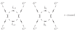
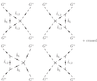
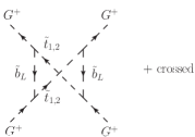
Figure 1: Stop-sbottom loop diagrams which induce $G^{+}G^{+}$ scattering. Time flows upward, and “crossed” means crossed diagram for final-state bosons. Circle-type, triangle-type, and crossed box-type diagrams correspond to ${\cal A}_{G^{+}G^{+}}^{\tilde{t}\mathchar 45\relax{\tilde{b}},{\rm cir}}$, ${\cal A}_{G^{+}G^{+}}^{\tilde{t}\mathchar 45\relax{\tilde{b}},{\rm tri}}$, and ${\cal A}_{G^{+}G^{+}}^{\tilde{t}\mathchar 45\relax{\tilde{b}},{\rm box}}$ in Eq. (14), respectively.

Let us discuss $G^{+}G^{+}\to G^{+}G^{+}$ scattering first. The scattering amplitudes in the supersymmetric model and the SM are given by the form

$${\cal A}_{G^{+}G^{+}}={\cal A}_{G^{+}G^{+}}^{\rm tree}+{\cal A}_{G^{+}G^{+}}^{t\mathchar 45\relax b}+{\cal A}_{G^{+}G^{+}}^{\tilde{t}\mathchar 45\relax{\tilde{b}}}\,,$$ (8)

$${\cal A}_{G^{+}G^{+}}^{\rm SM}={\cal A}_{G^{+}G^{+}}^{\rm SM,\,tree}+{\cal A}_{G^{+}G^{+}}^{{\rm SM},\,t\mathchar 45\relax b}\,,$$ (9)

where “tree”, “$t\mathchar 45\relax b$”, and “$\tilde{t}\mathchar 45\relax{\tilde{b}}$” indicate the tree-level amplitude, top-bottom loop amplitude, and stop-sbottom loop amplitude, respectively, which are given by

$${\cal A}_{G^{+}G^{+}}^{\rm tree} =-4\lambda_{\rm H}^{\rm SM^{\prime}}-\frac{g_{Z}^{2}}{2}\Bigl{[}\frac{t}{u}+\frac{u}{t}+1\Bigr{]}\,,$$ (10)

$${\cal A}_{G^{+}G^{+}}^{\rm SM,\,tree} =-4\lambda_{\rm H}^{\rm SM}-\frac{g_{Z}^{2}}{2}\Bigl{[}\frac{t}{u}+\frac{u}{t}+1\Bigr{]}\,,$$ (11)

$${\cal A}_{G^{+}G^{+}}^{t\mathchar 45\relax b} =-\frac{2N_{c}(y_{t}^{\rm SM^{\prime}})^{4}}{(4\pi)^{2}}\Bigl{[}B_{0}(t,m_{t}^{2},m_{t}^{2})+B_{0}(u,m_{t}^{2},m_{t}^{2})\Bigr{]}\,,$$ (12)

$${\cal A}_{G^{+}G^{+}}^{{\rm SM},\,t\mathchar 45\relax b} =-\frac{2N_{c}(y_{t}^{\rm SM})^{4}}{(4\pi)^{2}}\Bigl{[}B_{0}(t,m_{t}^{2},m_{t}^{2})+B_{0}(u,m_{t}^{2},m_{t}^{2})\Bigr{]}\,,$$ (13)

where $t=(p_{1}-k_{1})^{2}$, $u=(p_{1}-k_{2})^{2}$ ($p_{i}$ and $k_{i}$ ($i,j=1,2$) are momenta of incident and scattered particles, respectively), and $B_{0}$ is the loop function defined in Eq. (B.5) in Ref. Endo:2016koi without $1/\bar{\epsilon}$. The couplings are renormalized ones and their $\mu$ dependence is implicit. Here we have taken the leading terms in the $|t|,|u|\gg m_{Z}^{2}$ limit. ${\cal A}_{G^{+}G^{+}}^{\tilde{t}\mathchar 45\relax{\tilde{b}}}$ consists of three types of diagrams, circle, triangle and box types, which are shown in Fig. 1. We can derive them straightforwardly as

$${\cal A}_{G^{+}G^{+}}^{\tilde{t}\mathchar 45\relax{\tilde{b}}}={\cal A}_{G^{+}G^{+}}^{\tilde{t}\mathchar 45\relax{\tilde{b}},{\rm cir}}+{\cal A}_{G^{+}G^{+}}^{\tilde{t}\mathchar 45\relax{\tilde{b}},{\rm tri}}+{\cal A}_{G^{+}G^{+}}^{\tilde{t}\mathchar 45\relax{\tilde{b}},{\rm box}}\,,$$ (14)

with

$${\cal A}_{G^{+}G^{+}}^{\tilde{t}\mathchar 45\relax{\tilde{b}},{\rm cir}}= \frac{N_{C}(y_{t}^{\rm SM^{\prime}})^{4}}{(4\pi)^{2}}\Bigl{[}s^{4}_{\theta_{t}}B_{0}(t,m_{\tilde{t}_{1}}^{2},m_{\tilde{t}_{1}}^{2})+c^{4}_{\theta_{t}}B_{0}(t,m_{\tilde{t}_{2}}^{2},m_{\tilde{t}_{2}}^{2})+2s^{2}_{\theta_{t}}c^{2}_{\theta_{t}}B_{0}(t,m_{\tilde{t}_{1}}^{2},m_{\tilde{t}_{2}}^{2})+B_{0}(t,m_{\tilde{b}_{L}}^{2},m_{\tilde{b}_{L}}^{2})\Bigr{]}$$

$$\qquad\qquad\qquad+(t\to u~{}{\rm term})\,,$$ (15)

$${\cal A}_{G^{+}G^{+}}^{\tilde{t}\mathchar 45\relax{\tilde{b}},{\rm tri}}= \frac{2N_{C}(y_{t}^{\rm SM^{\prime}})^{4}X_{t}^{2}}{(4\pi)^{2}}\Bigl{[}s^{4}_{\theta_{t}}C_{0}(0,t,0,m_{\tilde{b}_{L}}^{2},m_{\tilde{t}_{1}}^{2},m_{\tilde{t}_{1}}^{2})+c^{4}_{\theta_{t}}C_{0}(0,t,0,m_{\tilde{b}_{L}}^{2},m_{\tilde{t}_{2}}^{2},m_{\tilde{t}_{2}}^{2})+2s^{2}_{\theta_{t}}c^{2}_{\theta_{t}}C_{0}(0,t,0,m_{\tilde{b}_{L}}^{2},m_{\tilde{t}_{1}}^{2},m_{\tilde{t}_{2}}^{2})$$

$$\qquad\qquad\qquad+s^{2}_{\theta_{t}}C_{0}(0,t,0,m_{\tilde{t}_{1}}^{2},m_{\tilde{b}_{L}}^{2},m_{\tilde{b}_{L}}^{2})+c^{2}_{\theta_{t}}C_{0}(0,t,0,m_{\tilde{t}_{2}}^{2},m_{\tilde{b}_{L}}^{2},m_{\tilde{b}_{L}}^{2})\Bigr{]}+(t\to u~{}{\rm term})\,,$$ (16)

$${\cal A}_{G^{+}G^{+}}^{\tilde{t}\mathchar 45\relax{\tilde{b}},{\rm box}}= \frac{2N_{C}(y_{t}^{\rm SM^{\prime}})^{4}X_{t}^{4}}{(4\pi)^{2}}\Bigl{[}s^{4}_{\theta_{t}}D_{0}(0,0,0,0,u,t,m_{\tilde{b}_{L}}^{2},m_{\tilde{t}_{1}}^{2},m_{\tilde{b}_{L}}^{2},m_{\tilde{t}_{1}}^{2})+c^{4}_{\theta_{t}}D_{0}(0,0,0,0,u,t,m_{\tilde{b}_{L}}^{2},m_{\tilde{t}_{2}}^{2},m_{\tilde{b}_{L}}^{2},m_{\tilde{t}_{2}}^{2})$$

$$\qquad\qquad\qquad+2s^{2}_{\theta_{t}}c^{2}_{\theta_{t}}D_{0}(0,0,0,0,u,t,m_{\tilde{b}_{L}}^{2},m_{\tilde{t}_{1}}^{2},m_{\tilde{b}_{L}}^{2},m_{\tilde{t}_{2}}^{2})\Bigr{]}\,.$$ (17)

Loop functions $C_{0}$ and $D_{0}$ are those defined in Ref. Hahn:1998yk . $m_{\tilde{b}_{L}}$ is the left-handed sbottom mass. Since we consider that the right-handed sbottom mass is much larger than the third-generation left-handed squark mass, the lighter sbottom is mostly composed of $b_{L}$; thus, $m_{\tilde{b}_{L}}\simeq m_{L}$. $\theta_{t}$ is the mixing angle in stop sector defined as $(\tilde{t}_{1},\tilde{t}_{2})^{T}=Z\,(\tilde{t}_{L},\tilde{t}_{R})^{T}$ with orthogonal matrix $Z_{11}=\cos\theta_{t}\equiv c_{\theta_{t}}$, $Z_{12}=\sin\theta_{t}\equiv s_{\theta_{t}}$. To be consistent with $\xi$ expansion analysis, we have omitted terms such as $(y_{t}^{\rm SM^{\prime}})^{2}g_{Z}^{2}$ and $g_{Z}^{4}$ in Eq. (15), which are $\xi^{3}$ and $\xi^{4}$, respectively, in $\xi$ expansion. We note that the explicit $\mu$ dependence coming from $B_{0}$ function is canceled at the leading order by the RG flow of $\lambda_{\rm H}^{\rm SM}$ ($\lambda_{\rm H}^{\rm SM^{\prime}}$). Since our goal is to compute the deviation at leading order in $\xi$ expansion, we take $\mu=m_{\tilde{t}}$ in the amplitude hereafter.

Another scattering amplitude for the process $G^{+}G^{-}\to G^{+}G^{-}$ can be obtained by replacing the Mandelstam variable $u$ by $s$.

Before going to the numerical analysis, let us check low- and high-energy limits. In the low-energy limit, the amplitudes ${\cal A}_{G^{+}G^{+}}$ and ${\cal A}_{G^{+}G^{-}}$ should coincide with those in the SM. To see this we define $\Delta{\cal A}_{G^{+}G^{\pm}}$

$$\Delta{\cal A}_{G^{+}G^{\pm}}={\cal A}_{G^{+}G^{\pm}}-{\cal A}_{G^{+}G^{\pm}}^{\rm SM}\,.$$ (18)

Then, using the matching conditions (3) and (4), they are simply given by

$$\Delta{\cal A}_{G^{+}G^{\pm}}={\cal A}_{G^{+}G^{\pm}}^{\tilde{t}\mathchar 45\relax{\tilde{b}}}+\frac{4N_{C}(y_{t}^{\rm SM}(m_{\tilde{t}}))^{4}}{(4\pi)^{2}}\frac{X_{t}^{2}}{m_{\tilde{t}}^{2}}\Bigl{(}1-\frac{X_{t}^{2}}{12m_{\tilde{t}}^{2}}\Bigr{)}\,,$$ (19)

In the low-energy limit, $s,|t|,|u|\ll m_{\tilde{t}}^{2}$ (but $s,|t|,|u|\gg m_{Z}^{2}$), and taking $m_{\tilde{t}_{1}}\simeq m_{\tilde{t}_{2}}\simeq m_{L}\simeq m_{\tilde{t}}$  the stop-sbottom loop contribution behaves as

$${\cal A}_{G^{+}G^{\pm}}^{\tilde{t}\mathchar 45\relax{\tilde{b}},{\rm cir}}\longrightarrow\frac{4N_{C}(y_{t}^{\rm SM^{\prime}}(\mu))^{4}}{(4\pi)^{2}}\log\Bigl{(}\frac{\mu^{2}}{m_{\tilde{t}}^{2}}\Bigr{)}\Bigr{|}_{\mu=m_{\tilde{t}}}\,,$$ (20)

$${\cal A}_{G^{+}G^{\pm}}^{\tilde{t}\mathchar 45\relax{\tilde{b}},{\rm tri}}\longrightarrow\frac{8N_{C}(y_{t}^{\rm SM^{\prime}}(\mu))^{4}X_{t}^{2}}{(4\pi)^{2}}\Bigl{(}-\frac{1}{2m^{2}_{\tilde{t}}}\Bigr{)}\Bigr{|}_{\mu=m_{\tilde{t}}}\,,$$ (21)

$${\cal A}_{G^{+}G^{\pm}}^{\tilde{t}\mathchar 45\relax{\tilde{b}},{\rm box}}\longrightarrow\frac{2N_{C}(y_{t}^{\rm SM^{\prime}}(\mu))^{4}X_{t}^{4}}{(4\pi)^{2}}\Bigl{(}\frac{1}{6m^{4}_{\tilde{t}}}\Bigr{)}\Bigr{|}_{\mu=m_{\tilde{t}}}\,,$$ (22)

which leads to

$${\cal A}_{G^{+}G^{\pm}}^{\tilde{t}\mathchar 45\relax{\tilde{b}}}\longrightarrow-\frac{4N_{C}(y_{t}^{\rm SM}(m_{\tilde{t}}))^{4}}{(4\pi)^{2}}\Bigl{[}\frac{X_{t}^{2}}{m^{2}_{\tilde{t}}}\Bigl{(}1-\frac{X_{t}^{2}}{12m^{2}_{\tilde{t}}}\Bigr{)}\Bigr{]}\,.$$ (23)

Thus $\Delta{\cal A}_{G^{+}G^{-}}\to 0$, which means that the amplitude asymptotically approaches the SM one in the low-energy limit as expected.

In numerical calculation $m_{\tilde{t}_{1}}\simeq m_{\tilde{t}_{2}}\simeq m_{\tilde{t}}$ is not always satisfied. Therefore, in the later analysis, we use the following expressions instead of Eqs. (19) and (3);

$$\Delta{\cal A}_{G^{+}G^{\pm}}={\cal A}_{G^{+}G^{\pm}}^{\tilde{t}\mathchar 45\relax{\tilde{b}}}-{\cal A}_{G^{+}G^{\pm}}^{\tilde{t}\mathchar 45\relax{\tilde{b}}}|_{s\to 0}\,,$$ (24)

$$\lambda_{\rm H}^{\rm SM}(\mu_{\tilde{t}})=\lambda_{\rm H}^{\rm SM^{\prime}}(\mu_{\tilde{t}})-\frac{1}{4}{\cal A}_{G^{+}G^{\pm}}^{\tilde{t}\mathchar 45\relax{\tilde{b}}}|_{s\to 0}\,.$$ (25)

In the high-energy limit $s,|t|,|u|\gg m_{\tilde{t}},|X_{t}|$, on the other hand,

$${\cal A}_{G^{+}G^{+}}^{\tilde{t}\mathchar 45\relax{\tilde{b}}}\longrightarrow \frac{4N_{C}(y_{t}^{\rm SM^{\prime}}(m_{\tilde{t}}))^{4}}{(4\pi)^{2}}\Bigl{[}\log\Bigl{(}\frac{m^{2}_{\tilde{t}}}{\sqrt{tu}}\Bigr{)}-2+\frac{m^{2}_{\tilde{t}}}{t}\Bigl{(}\log\frac{m^{2}_{\tilde{t}}}{-t}-1\Bigr{)}+\frac{m^{2}_{\tilde{t}}}{u}\Bigl{(}\log\frac{m^{2}_{\tilde{t}}}{-u}-1\Bigr{)}$$

$$\qquad\qquad\qquad+\frac{X_{t}^{2}}{2t}\log^{2}\Bigl{(}\frac{m^{2}_{\tilde{t}}}{-t}\Bigr{)}+\frac{X_{t}^{2}}{2u}\log^{2}\Bigl{(}\frac{m^{2}_{\tilde{t}}}{-u}\Bigl{)}\Bigr{]}+{\cal O}\Bigl{(}\frac{m^{4}_{\tilde{t}},X_{t}^{4}}{|t|^{2},|u|^{2}}\Bigr{)}\,,$$ (26)

$${\cal A}_{G^{+}G^{-}}^{\tilde{t}\mathchar 45\relax{\tilde{b}}}\longrightarrow \frac{2N_{C}(y_{t}^{\rm SM^{\prime}}(m_{\tilde{t}}))^{4}}{(4\pi)^{2}}\Bigl{[}\log\Bigl{(}\frac{m^{2}_{\tilde{t}}}{\sqrt{-st}}\Bigr{)}-2+\frac{m^{2}_{\tilde{t}}}{s}\Bigl{(}\log\frac{m^{2}_{\tilde{t}}}{s}-1\Bigr{)}+\frac{m^{2}_{\tilde{t}}}{t}\Bigl{(}\log\frac{m^{2}_{\tilde{t}}}{-t}-1\Bigr{)}-\frac{i\pi}{2}\Bigl{(}1-2\frac{m^{2}_{\tilde{t}}}{s}\Bigr{)}$$

$$\qquad\qquad\qquad+\frac{X_{t}^{2}}{2s}\Bigl{\{}\log^{2}\Bigl{(}\frac{m^{2}_{\tilde{t}}}{s}\Bigl{)}-\pi^{2}+2i\pi\log\Bigl{(}\frac{m^{2}_{\tilde{t}}}{s}\Bigl{)}\Bigr{\}}+\frac{X_{t}^{2}}{2t}\log^{2}\Bigl{(}\frac{m^{2}_{\tilde{t}}}{-t}\Bigr{)}\Bigr{]}+{\cal O}\Bigl{(}\frac{m^{4}_{\tilde{t}},X_{t}^{4}}{s^{2},|t|^{2}}\Bigr{)}\,.$$ (27)

The first line on the right-hand side comes from circle diagram, which agrees with the native estimation (6) and can be understood in terms of the RG flow of the Higgs quartic coupling. Meanwhile, the others are derived in the explicit calculation of Feynman diagrams, which cannot be described by the RG equations and are necessary ingredients for the numerical analysis of the scattering processes.

IV Numerical results

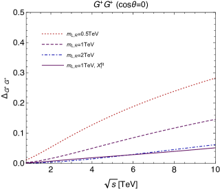
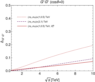
Figure 2: Deviation from the SM for the $G^{+}G^{+}$ scattering process, defined in Eq. (28), as a function of center-of-mass energy $\sqrt{s}$. The scattering angle is taken as $\cos\theta=0$. (Left) $m_{L}=m_{R}=0.5$ (red dotted), 1 (purple dashed), and 2 (blue dot-dashed) TeV with $X_{t}=0.5m_{L}$ at $\mu=m_{\tilde{t}}$. In $X_{t}^{\rm fit}$ (purple solid) line, $X_{t}=1.82$ TeV, which gives the observed Higgs mass for $m_{L}=m_{R}=1$ TeV, is taken. (Right) $m_{L}=2m_{R}=1$ (red dotted) and 2 (purple dashed) TeV with $X_{t}=0.5m_{L}$ at $\mu=m_{\tilde{t}}$. In $X_{t}^{\rm fit}$ (red solid) line, $X_{t}=1.45$ TeV, which gives the observed Higgs mass, is taken.

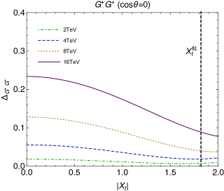
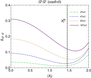
Figure 3: $X_{t}$ and $\sqrt{s}$ dependence of the amplitude for $G^{+}G^{+}$ process. $m_{L}=m_{R}=1$ TeV (left) and $m_{L}=2m_{R}=1$ TeV (right) are taken. Line contents are $\sqrt{s}=2$ (green dot-dashed), $4$ (blue dashed), $8$ (orange dotted), and $16$ TeV (purple solid). Locations of $X_{t}^{\rm fit}$ are also indicated.

Now we are ready to give the numerical result. To this end, we use the quantity:

$$\Delta_{G^{+}G^{\pm}}=\frac{|{\cal A}_{G^{+}G^{\pm}}|^{2}-|{\cal A}_{G^{+}G^{\pm}}^{\rm SM}|^{2}}{|{\cal A}_{G^{+}G^{\pm}}^{\rm SM}|^{2}}\,,$$ (28)

which corresponds to the deviation from the SM for the differential cross section.

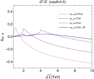
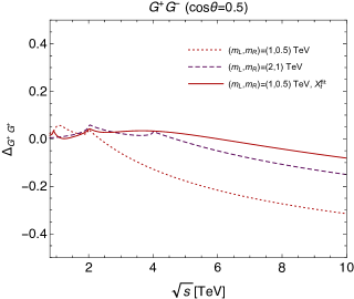
Figure 4: Same as Fig. 2 but for $G^{+}G^{-}$ scattering process taking $\cos\theta=0.5$.

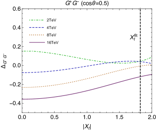
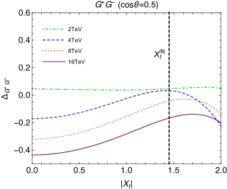
Figure 5: Same as Fig. 3 but for $G^{+}G^{-}$ process taking $\cos\theta=0.5$.

Fig. 2 shows the result for the $G^{+}G^{+}$ process as a function of $\sqrt{s}$ for the fixed scattering angle, $\cos\theta=0$. We take $m_{L}=m_{R}=0.5$, 1, and 2 TeV (left) and $m_{L}=2m_{R}=1$ and 2 TeV (right) with $X_{t}=0.5m_{L}$ at $\mu=m_{\tilde{t}}$, which corresponds to scenario (b) discussed in Sec. II. Roughly speaking, left (right) panel covers the situation of the degenerate (split) mass spectrum in the stop sector. For scenario (a), the results for $m_{L}=m_{R}=1$ TeV with $X_{t}=X_{t}^{\rm fit}=1.82~{}{\rm TeV}$ (left), $m_{L}=2m_{R}=1$ TeV with $X_{t}=X_{t}^{\rm fit}=1.45~{}{\rm TeV}$ (right) are given. Here we omit another larger value of $|X_{t}|$ to give the observed Higgs mass since it would not be phenomenologically acceptable due to vacuum instability bound $X_{t}/\sqrt{m_{\tilde{t}_{1}}^{2}+m_{\tilde{t}_{2}}^{2}}\lesssim\sqrt{3}$ Blinov:2013fta (see also the earlier analysis to give the bound $X_{t}/\sqrt{m_{\tilde{t}_{1}}^{2}+m_{\tilde{t}_{2}}^{2}}\lesssim\sqrt{7}$ Kusenko:1996jn .)

It is seen that the deviation increases monotonically as $\sqrt{s}$ gets large for fixed $m_{L,R}$ and $X_{t}$. It is attributed to the logarithmic term (first term of Eq. (26)), which originates in the stop-sbottom loop and can be understood by RG running of the Higgs quartic coupling. A smaller $m_{L,R}$ gives a larger deviation. For example, $\Delta_{G^{+}G^{+}}=$16 (28)%, 7 (15)%, and 2 (6)% for $\sqrt{s}=5$ (10) TeV for $m_{L,R}=0.5$, 1, and 2 TeV with $X_{t}=0.5m_{L}$, respectively. This is because the $\log(m^{2}_{\tilde{t}}/\sqrt{tu})$ term, which is dominant in ${\cal A}_{G^{+}G^{+}}^{\tilde{t}\mathchar 45\relax{\tilde{b}}}$ (see Eq. (26)), contributes constructively in the total amplitude for $\sqrt{s}>m_{\tilde{t}}$. It is true for the split mass spectrum (right panel).

When $X_{t}=X_{t}^{\rm fit}$, on the other hand, $\Delta_{G^{+}G^{+}}$ gets smaller compared to the result with the same $m_{L,R}$ but $X_{t}=0.5m_{L}$. To understand the behavior, we plot $\Delta_{G^{+}G^{+}}$ as a function of $X_{t}$ for various $\sqrt{s}$ in Fig. 3 for $m_{L}=m_{R}=1$ TeV (left) and $m_{L}=2m_{R}=1$ TeV (right). It is found that $\Delta_{G^{+}G^{+}}$ decreases as $X_{t}$ increases for $X_{t}\lesssim X_{t}^{\rm fit}$, which can be understood from Eqs. (24) (or (19)) and (26). The second term on the right-hand side of Eq. (24) is positive and destructively interferes with ${\cal A}_{G^{+}G^{+}}^{\tilde{t}\mathchar 45\relax{\tilde{b}}}$ for $X_{t}\lesssim X_{t}^{\rm fit}(\sim m_{\tilde{t}})$.

For larger $|\cos\theta|$ the deviation gets smaller since $Z$ and $\gamma$ exchange terms which are proportional to $1/u$ or $1/t$ dominate the scattering amplitude. For example, when $\cos\theta=0.5$, $\Delta_{G^{+}G^{+}}=$ 11 (18)%, 4.8 (10)%, and 2 (4)% for $\sqrt{s}=5$ (10) TeV $m_{L}=m_{R}=0.5$, 1, and 2 TeV with $X_{t}=0.5m_{L}$, respectively.

$G^{+}G^{-}$ scattering has similar behavior except for a bump, which corresponds to a resonance at $\sqrt{s}\simeq 2m_{\tilde{t}}$ in Fig. 4. This bump is due to discontinuity of the first derivative of $B_{0}(q^{2},m_{1}^{2},m_{2}^{2})$ with respect to $q^{2}$ at $q^{2}\simeq(m_{1}+m_{2})^{2}$. For $\sqrt{s}\lesssim 2m_{\tilde{t}}$, the stop-sbottom loop (dominated by circle diagrams) is positive, which constructively interferes with tree plus top-bottom loop contributions. In the region $\sqrt{s}\gtrsim 2m_{\tilde{t}}$, on the other hand, $\Delta_{G^{+}G^{-}}$ monotonically decreases. This is because the dominant term $\log(m^{2}_{\tilde{t}}/\sqrt{-st})$ in Eq. (27) is negative, which is destructive in the total amplitude at the high energy range. For example, $\Delta_{G^{+}G^{-}}=-29$ ($-42$)%, $-11$ ($-25$)%, and $6$ ($-9$)% for $\sqrt{s}=5$ (10) TeV and $\cos\theta=0.5$ for $m_{L}=m_{R}=0.5$, 1, and 2 TeV with $X_{t}=0.5m_{L}$, respectively (left panel). Qualitatively the same behavior is seen for the split mass case (right panel). Regarding $X_{t}$ dependence, it is seen that $|\Delta_{G^{+}G^{-}}|$ gets smaller for $X_{t}=X_{t}^{\rm fit}$ similarly to the $G^{+}G^{+}$ case. Fig. 5 clarifies the behavior. It is found that $|\Delta_{G^{+}G^{-}}|$ decreases in the $X_{t}\lesssim m_{\tilde{t}}$ region, which to attributed to the second term on the right-hand side of Eq. (24) as explained in the $G^{+}G^{+}$ case.

Thus, in both the $G^{+}G^{+}$ and $G^{+}G^{-}$ scattering processes, it would be difficult to observe the deviation from the SM in the parameter space $|X_{t}|\sim m_{\tilde{t}}$, especially $X_{t}\simeq X_{t}^{\rm fit}$, since $\Delta_{G^{+}G^{\pm}}$ is a few percent. In other words, scenario (a) is like a “blind spot” for the TeV-scale stop search in the longitudinal $W$ boson scattering processes. In scenario (b), on the other hand, ${\cal O}$(1–10%) deviation is expected for $\sqrt{s}=1$–$10$ TeV.

V concluding remarks

In this paper we have studied high energy longitudinal $W$ boson scattering with a light scalar top of which the mass is a few hundred GeV to a few TeV. They affect the SM Higgs potential at quantum level, and consequently the deviation from the standard model in longitudinal gauge boson scattering is expected from the equivalence theorem. Applying the equivalence theorem, we have computed charged Nambu-Goldstone boson scattering processes and substituted them as high energy $W^{+}_{L}W^{\pm}_{L}$ scattering processes. In the study, we consider two scenarios: (a) Higgs mass is explained in the MSSM particle contents, and (b) other contributions besides the MSSM particles make the observed Higgs mass. It has been found that ${\cal O}$(1–10%) deviation in the differential cross section is predicted depending on stop mass and kinematics. As an example of scenario (b), for $\sqrt{s}=5$ (10) TeV and $\cos\theta=0$, the deviation in the $W^{+}_{L}W^{+}_{L}$ process is 16 (28)% and 7 (15)% when both left- and right-handed stop masses ($m_{L}$ and $m_{R}$) are 0.5 and 1 TeV with the mixing parameter $X_{t}=0.5m_{L}$, respectively. Similarly, in $W^{+}_{L}W^{-}_{L}$, it is $-29$ ($-42$)%, and $-11$ ($-25$)% but for $\cos\theta=0.5$. For scenario (a), on the contrary, it has been discovered that the deviation gets smaller, e.g., $2$ ($4$)% and $4$ ($-4$)% for $m_{L}=m_{R}=1$ TeV with the appropriate $X_{t}$ for $\sqrt{s}=5$ (10) in $W^{+}_{L}W^{+}_{L}$ and $W^{+}_{L}W^{-}_{L}$, respectively. The same behavior is seen for the $m_{L}\neq m_{R}$ case. Thus in such a case it would be challenging to see the existence of stop in $W_{L}W_{L}$ scattering.

High energy longitudinal gauge boson scattering has started to be measured at the LHC Aad:2014zda ; Khachatryan:2014sta . However, the observation of ${\cal O}(10\%)$ deviation would be difficult even in Run 2 at the LHC. This is because the number of events which has over a few TeV invariant mass of $W$ boson system is suppressed due to gauge cancellation Accomando:2006mc . (We have checked this by using the MadGraph package Alwall:2014hca .) Thus at least an upgraded program, such as the High Luminosity LHC, would be necessary. Or the Future Circular Collider, which is planed to operate at 100 TeV center-of-mass energy, would be more promising for the study of the gauge boson scattering. In such a high energy experiment, the observation of stop or sbottom pair production might be more direct and easier way to observe a clue of the supersymmetry. As mentioned in the Introduction, however, there are model dependence in the data analysis, e.g., details of the decay modes, or violation of R-parity. High energy longitudinal gauge boson scattering would be complementary to the direct searches. We have provided the theoretical ingredients for the numerical study and discuss feasibility for the discovery of scalar tops in the longitudinal gauge boson scattering. The next step will be to perform full simulation for hadron or lepton collider experiments with various energies, for which Refs. Denner:1996ug ; Denner:1997kq ; Biedermann:2016yds ; Borel:2012by ; Alboteanu:2008my ; Accomando:2006hq ; Bernreuther:2015llj ; Fleper:2016frz ; Bishara:2016kjn ; Doroba:2012pd ; Kilian:2014zja ; Kilian:2015opv are useful. We leave it to future work.

Acknowledgements

We are grateful to Kazuhiro Endo and Yukinari Sumino for valuable discussions. This work was supported by MEXT KAKENHI Grant Number 17H05402 and JSPS KAKENHI Grant Number 17K14278. (K.I.)

Appendix A Analytic check

We will check that the $G^{+}G^{+}$ and $G^{+}G^{-}$ scattering amplitudes reduce to those in the SM in the low-energy limit by using the analytic Higgs mass formula for the $\tilde{m}\sim m_{\tilde{t}}$ case.

First of all we need to use the Lagrangian after the following replacement:

$$\lambda_{\rm H}^{\rm SM^{\prime}}\to(1/8)g_{Z}^{2}\cos^{2}2\beta\,,\,\,\,\,y_{t}^{\rm SM^{\prime}}\to\lambda_{t}\sin\beta\,.$$ (29)

Consequently, the matching conditions are

$$\lambda_{\rm H}^{\rm SM}(\mu_{\tilde{t}})=\frac{1}{8}g_{Z}^{2}\cos^{2}2\beta(\mu_{\tilde{t}})$$

$$\qquad+\frac{N_{C}(y_{t}^{{\rm SM^{\prime}}}(\mu_{\tilde{t}}))^{4}}{(4\pi)^{2}}\Bigl{[}-\log\Bigl{(}\frac{\mu^{2}_{\tilde{t}}}{m_{\tilde{t}}^{2}}\Bigr{)}+\frac{X_{t}^{2}}{m_{\tilde{t}}^{2}}\Bigl{(}1-\frac{X_{t}^{2}}{12m_{\tilde{t}}^{2}}\Bigr{)}\Bigr{]}\,,$$ (30)

$$y_{t}^{\rm SM}(\mu_{\tilde{t}})=\lambda_{t}\sin\beta(\mu_{\tilde{t}})\,.$$ (31)

In the MSSM where $\tilde{m}\sim m_{\tilde{t}}$, the SM Higgs mass is given by analytically using the effective potential Haber:1990aw ; Ellis:1990nz ; Ellis:1991zd ; Okada:1990vk

$$(m_{h}^{{\rm MSSM}})^{2}\simeq m_{Z}^{2}\cos^{2}2\beta$$

$$+\frac{2N_{c}(\lambda_{t}\sin\beta)^{4}v^{2}}{(4\pi)^{2}}\Bigl{[}\log\Bigl{(}\frac{m_{\tilde{t}}^{2}}{m_{t}^{2}}\Bigr{)}+\frac{X_{t}^{2}}{m_{\tilde{t}}^{2}}\Bigl{(}1-\frac{X_{t}^{2}}{12m_{\tilde{t}}^{2}}\Bigr{)}\Bigr{]}\,.$$ (32)

Using this expression, it is found that the $X_{t}$ dependence on $m_{h}^{{\rm MSSM}}$ and the one obtained by using the RG equation in the text agree within around 1 GeV when we take $\mu=m_{\tilde{t}}$ for top Yukawa coupling. Hereafter, we take $\mu=m_{\tilde{t}}$.

$G^{+}G^{+}$ and $G^{+}G^{-}$ scattering amplitudes are easily obtained by using the previous result along with the above replacement and matching conditions. Now let us see the low-energy limit, $s,|t|,|u|\ll m_{\tilde{t}}^{2}$ (but $s,|t|,|u|\gg m_{Z}^{2}$). ${\cal A}_{G^{+}G^{\pm}}^{\tilde{t}\mathchar 45\relax{\tilde{b}}}$ corresponding to Eq. (23) is the same expression. Then, combining with

$${\cal A}_{G^{+}G^{+}}^{t\mathchar 45\relax b}\longrightarrow-\frac{4N_{c}(y_{t}^{\rm SM})^{4}}{(4\pi)^{2}}\Bigl{[}\log\Bigl{(}\frac{\mu^{2}}{\sqrt{tu}}\Bigr{)}+2\Bigr{]}\Bigr{|}_{\mu=m_{\tilde{t}}}\,,$$ (33)

$${\cal A}_{G^{+}G^{-}}^{t\mathchar 45\relax b}\longrightarrow-\frac{4N_{c}(y_{t}^{\rm SM})^{4}}{(4\pi)^{2}}\Bigl{[}\log\Bigl{(}\frac{\mu^{2}}{\sqrt{st}}\Bigr{)}+2\Bigr{]}\Bigr{|}_{\mu=m_{\tilde{t}}}\,,$$ (34)

and Eq. (32), we obtain

$${\cal A}_{G^{+}G^{+}}\longrightarrow -\frac{2(m_{h}^{{\rm MSSM}})^{2}}{v^{2}}-\frac{g_{Z}^{2}}{2}\Bigl{[}\frac{t}{u}+\frac{u}{t}+1\Bigr{]}$$

$$-\frac{2N_{c}(y_{t}^{\rm SM})^{4}}{(4\pi)^{2}}\Bigl{[}\log\Bigl{(}\frac{m_{t}^{4}}{tu}\Bigr{)}+4\Bigr{]}\,,$$ (35)

$${\cal A}_{G^{+}G^{-}}\longrightarrow -\frac{2(m_{h}^{{\rm MSSM}})^{2}}{v^{2}}-\frac{g_{Z}^{2}}{2}\Bigl{[}\frac{s}{t}+\frac{t}{s}+1\Bigr{]}$$

$$-\frac{2N_{c}(y_{t}^{\rm SM})^{4}}{(4\pi)^{2}}\Bigl{[}\log\Bigl{(}\frac{m_{t}^{4}}{st}\Bigr{)}+4\Bigr{]}\,.$$ (36)

This is exactly the amplitude including top-bottom loop in the SM for $m_{h}^{\rm MSSM}=m_{h}$ Endo:2016koi .

References

- (1) G. Aad et al. [ATLAS Collaboration], Phys. Lett. B 716, 1 (2012) doi:10.1016/j.physletb.2012.08.020 [arXiv:1207.7214 [hep-ex]].
- (2) S. Chatrchyan et al. [CMS Collaboration], Phys. Lett. B 716, 30 (2012) doi:10.1016/j.physletb.2012.08.021 [arXiv:1207.7235 [hep-ex]].
- (3) The ATLAS and CMS Collaborations, ATLAS-CONF-2015-044.
- (4) H. E. Haber and R. Hempfling, Phys. Rev. Lett. 66, 1815 (1991). doi:10.1103/PhysRevLett.66.1815
- (5) J. R. Ellis, G. Ridolfi and F. Zwirner, Phys. Lett. B 257, 83 (1991). doi:10.1016/0370-2693(91)90863-L
- (6) J. R. Ellis, G. Ridolfi and F. Zwirner, Phys. Lett. B 262, 477 (1991). doi:10.1016/0370-2693(91)90626-2
- (7) Y. Okada, M. Yamaguchi and T. Yanagida, Prog. Theor. Phys. 85, 1 (1991). doi:10.1143/PTP.85.1
- (8) Y. Okada, M. Yamaguchi and T. Yanagida, Phys. Lett. B 262, 54 (1991). doi:10.1016/0370-2693(91)90642-4
- (9) A. Brignole, Phys. Lett. B 281, 284 (1992). doi:10.1016/0370-2693(92)91142-V
- (10) D. Chway, T. H. Jung, H. D. Kim and R. Dermisek, Phys. Rev. Lett. 113, no. 5, 051801 (2014) doi:10.1103/PhysRevLett.113.051801 [arXiv:1308.0891 [hep-ph]].
- (11) K. Endo and Y. Sumino, JHEP 1505, 030 (2015) doi:10.1007/JHEP05(2015)030 [arXiv:1503.02819 [hep-ph]].
- (12) K. Hashino, S. Kanemura and Y. Orikasa, Phys. Lett. B 752, 217 (2016) doi:10.1016/j.physletb.2015.11.044 [arXiv:1508.03245 [hep-ph]].
- (13) K. Endo, K. Ishiwata and Y. Sumino, Phys. Rev. D 94, no. 7, 075007 (2016) doi:10.1103/PhysRevD.94.075007 [arXiv:1601.00696 [hep-ph]].
- (14) G. Aad et al. [ATLAS Collaboration], Eur. Phys. J. C 75, no. 10, 510 (2015) Erratum: [Eur. Phys. J. C 76, no. 3, 153 (2016)] doi:10.1140/epjc/s10052-015-3726-9, 10.1140/epjc/s10052-016-3935-x [arXiv:1506.08616 [hep-ex]].
- (15) The ATLAS collaboration [ATLAS Collaboration], ATLAS-CONF-2016-07; ATLAS-CONF-2016-050; ATLAS-CONF-2016-076.
- (16) M. Aaboud et al. [ATLAS Collaboration], Phys. Rev. D 94, no. 3, 032005 (2016) doi:10.1103/PhysRevD.94.032005 [arXiv:1604.07773 [hep-ex]].
- (17) CMS Collaboration [CMS Collaboration], CMS-PAS-SUS-16-014; CMS-PAS-SUS-16-015; CMS-PAS-SUS-16-028; CMS-PAS-SUS-16-029; CMS-PAS-SUS-16-030.
- (18) V. Khachatryan et al. [CMS Collaboration], Eur. Phys. J. C 76, no. 8, 460 (2016) doi:10.1140/epjc/s10052-016-4292-5 [arXiv:1603.00765 [hep-ex]].
- (19) S. Chatrchyan et al. [CMS Collaboration], Phys. Rev. Lett. 111, no. 22, 221801 (2013) doi:10.1103/PhysRevLett.111.221801 [arXiv:1306.6643 [hep-ex]].
- (20) V. Khachatryan et al. [CMS Collaboration], Phys. Lett. B 760, 178 (2016) doi:10.1016/j.physletb.2016.06.039 [arXiv:1602.04334 [hep-ex]].
- (21) G. Aad et al. [ATLAS Collaboration], JHEP 1606, 067 (2016) doi:10.1007/JHEP06(2016)067 [arXiv:1601.07453 [hep-ex]].
- (22) The ATLAS collaboration [ATLAS Collaboration], ATLAS-CONF-2016-022; ATLAS-CONF-2016-084.
- (23) A. Pierce and B. Shakya, arXiv:1611.00771 [hep-ph].
- (24) H. Baer, V. Barger, N. Nagata and M. Savoy, arXiv:1611.08511 [hep-ph].
- (25) M. Chala, A. Delgado, G. Nardini and M. Quiros, arXiv:1702.07359 [hep-ph].
- (26) J. Fan, M. Reece and L. T. Wang, JHEP 1508, 152 (2015) doi:10.1007/JHEP08(2015)152 [arXiv:1412.3107 [hep-ph]].
- (27) T. Moroi and Y. Okada, Mod. Phys. Lett. A 7, 187 (1992). doi:10.1142/S0217732392000124
- (28) T. Moroi and Y. Okada, Phys. Lett. B 295, 73 (1992). doi:10.1016/0370-2693(92)90091-H
- (29) K. S. Babu, I. Gogoladze and C. Kolda, hep-ph/0410085.
- (30) K. S. Babu, I. Gogoladze, M. U. Rehman and Q. Shafi, Phys. Rev. D 78, 055017 (2008) doi:10.1103/PhysRevD.78.055017 [arXiv:0807.3055 [hep-ph]].
- (31) S. P. Martin, Phys. Rev. D 81, 035004 (2010) doi:10.1103/PhysRevD.81.035004 [arXiv:0910.2732 [hep-ph]].
- (32) M. Asano, T. Moroi, R. Sato and T. T. Yanagida, Phys. Lett. B 705, 337 (2011) doi:10.1016/j.physletb.2011.10.025 [arXiv:1108.2402 [hep-ph]].
- (33) M. Endo, K. Hamaguchi, S. Iwamoto and N. Yokozaki, Phys. Rev. D 84, 075017 (2011) doi:10.1103/PhysRevD.84.075017 [arXiv:1108.3071 [hep-ph]].
- (34) J. L. Evans, M. Ibe and T. T. Yanagida, arXiv:1108.3437 [hep-ph].
- (35) T. Moroi, R. Sato and T. T. Yanagida, Phys. Lett. B 709, 218 (2012) doi:10.1016/j.physletb.2012.02.012 [arXiv:1112.3142 [hep-ph]].
- (36) M. Endo, K. Hamaguchi, S. Iwamoto and N. Yokozaki, Phys. Rev. D 85, 095012 (2012) doi:10.1103/PhysRevD.85.095012 [arXiv:1112.5653 [hep-ph]].
- (37) J. Hisano, W. Kuramoto and T. Kuwahara, arXiv:1611.07670 [hep-ph].
- (38) G. F. Giudice and A. Romanino, Nucl. Phys. B 699, 65 (2004) Erratum: [Nucl. Phys. B 706, 487 (2005)] doi:10.1016/j.nuclphysb.2004.11.048, 10.1016/j.nuclphysb.2004.08.001 [hep-ph/0406088].
- (39) D. Buttazzo, G. Degrassi, P. P. Giardino, G. F. Giudice, F. Sala, A. Salvio and A. Strumia, JHEP 1312, 089 (2013) doi:10.1007/JHEP12(2013)089 [arXiv:1307.3536 [hep-ph]].
- (40) H. E. Haber and R. Hempfling, Phys. Rev. D 48, 4280 (1993) doi:10.1103/PhysRevD.48.4280 [hep-ph/9307201].
- (41) M. Drees, R. Godbole and P. Roy, “Theory and Phenomenology of Sparticles: An Account of Four-Dimensional N=1 Supersymmetry in High Energy Physics”, World Scientific Publishing Company (2004).
- (42) S. Heinemeyer, W. Hollik and G. Weiglein, Comput. Phys. Commun. 124, 76 (2000) doi:10.1016/S0010-4655(99)00364-1 [hep-ph/9812320]; S. Heinemeyer, W. Hollik and G. Weiglein, Eur. Phys. J. C 9, 343 (1999) doi:10.1007/s100529900006, 10.1007/s100520050537 [hep-ph/9812472].
- (43) G. Aad et al. [ATLAS Collaboration], Phys. Rev. D 90, no. 5, 052004 (2014) [arXiv:1406.3827 [hep-ex]].
- (44) V. Khachatryan et al. [CMS Collaboration], Eur. Phys. J. C 74 (2014) 10, 3076 [arXiv:1407.0558 [hep-ex]].
- (45) V. S. Fadin, L. N. Lipatov, A. D. Martin and M. Melles, Phys. Rev. D 61, 094002 (2000) doi:10.1103/PhysRevD.61.094002 [hep-ph/9910338].
- (46) J. H. Kuhn, F. Metzler, A. A. Penin and S. Uccirati, JHEP 1106, 143 (2011) doi:10.1007/JHEP06(2011)143 [arXiv:1101.2563 [hep-ph]].
- (47) A. Denner and T. Hahn, Nucl. Phys. B 525, 27 (1998) doi:10.1016/S0550-3213(98)00287-9 [hep-ph/9711302].
- (48) A. Denner and S. Dittmaier, Nucl. Phys. Proc. Suppl. 160, 22 (2006) doi:10.1016/j.nuclphysbps.2006.09.025 [hep-ph/0605312].
- (49) E. Accomando, A. Denner and S. Pozzorini, JHEP 0703, 078 (2007) doi:10.1088/1126-6708/2007/03/078 [hep-ph/0611289].
- (50) T. Hahn and M. Perez-Victoria, Comput. Phys. Commun. 118, 153 (1999) doi:10.1016/S0010-4655(98)00173-8 [hep-ph/9807565].
- (51) N. Blinov and D. E. Morrissey, JHEP 1403, 106 (2014) doi:10.1007/JHEP03(2014)106 [arXiv:1310.4174 [hep-ph]].
- (52) A. Kusenko, P. Langacker and G. Segre, Phys. Rev. D 54, 5824 (1996) doi:10.1103/PhysRevD.54.5824 [hep-ph/9602414].
- (53) V. Barger, P. Huang, M. Ishida and W. Y. Keung, Phys. Lett. B 718, 1024 (2013) doi:10.1016/j.physletb.2012.11.049 [arXiv:1206.1777 [hep-ph]].
- (54) C. S. Lim, T. Inami and N. Sakai, Phys. Rev. D 29, 1488 (1984). doi:10.1103/PhysRevD.29.1488
- (55) M. Drees and K. Hagiwara, Phys. Rev. D 42, 1709 (1990). doi:10.1103/PhysRevD.42.1709
- (56) S. Heinemeyer, W. Hollik and G. Weiglein, Phys. Rept. 425, 265 (2006) doi:10.1016/j.physrep.2005.12.002 [hep-ph/0412214].
- (57) G. Aad et al. [ATLAS and CMS Collaborations], JHEP 1608, 045 (2016) doi:10.1007/JHEP08(2016)045 [arXiv:1606.02266 [hep-ex]].
- (58) A. Djouadi, Phys. Rept. 457, 1 (2008) doi:10.1016/j.physrep.2007.10.004 [hep-ph/0503172].
- (59) A. Djouadi, Phys. Rept. 459, 1 (2008) doi:10.1016/j.physrep.2007.10.005 [hep-ph/0503173].
- (60) G. Aad et al. [ATLAS Collaboration], Phys. Rev. Lett. 113, no. 14, 141803 (2014) doi:10.1103/PhysRevLett.113.141803 [arXiv:1405.6241 [hep-ex]].
- (61) V. Khachatryan et al. [CMS Collaboration], Phys. Rev. Lett. 114, no. 5, 051801 (2015) doi:10.1103/PhysRevLett.114.051801 [arXiv:1410.6315 [hep-ex]].
- (62) E. Accomando, A. Ballestrero, A. Belhouari and E. Maina, Phys. Rev. D 74, 073010 (2006) doi:10.1103/PhysRevD.74.073010 [hep-ph/0608019].
- (63) J. Alwall et al., JHEP 1407, 079 (2014) doi:10.1007/JHEP07(2014)079 [arXiv:1405.0301 [hep-ph]].
- (64) A. Denner, S. Dittmaier and T. Hahn, Phys. Rev. D 56, 117 (1997) doi:10.1103/PhysRevD.56.117 [hep-ph/9612390].
- (65) B. Biedermann, A. Denner and M. Pellen, arXiv:1611.02951 [hep-ph].
- (66) P. Borel, R. Franceschini, R. Rattazzi and A. Wulzer, JHEP 1206, 122 (2012) doi:10.1007/JHEP06(2012)122 [arXiv:1202.1904 [hep-ph]].
- (67) A. Alboteanu, W. Kilian and J. Reuter, JHEP 0811, 010 (2008) doi:10.1088/1126-6708/2008/11/010 [arXiv:0806.4145 [hep-ph]].
- (68) W. Bernreuther and L. Chen, Phys. Rev. D 93, no. 5, 053018 (2016) doi:10.1103/PhysRevD.93.053018 [arXiv:1511.07706 [hep-ph]].
- (69) C. Fleper, W. Kilian, J. Reuter and M. Sekulla, arXiv:1607.03030 [hep-ph].
- (70) F. Bishara, R. Contino and J. Rojo, arXiv:1611.03860 [hep-ph].
- (71) K. Doroba, J. Kalinowski, J. Kuczmarski, S. Pokorski, J. Rosiek, M. Szleper and S. Tkaczyk, Phys. Rev. D 86, 036011 (2012) doi:10.1103/PhysRevD.86.036011 [arXiv:1201.2768 [hep-ph]].
- (72) W. Kilian, T. Ohl, J. Reuter and M. Sekulla, Phys. Rev. D 91, 096007 (2015) doi:10.1103/PhysRevD.91.096007 [arXiv:1408.6207 [hep-ph]].
- (73) W. Kilian, T. Ohl, J. Reuter and M. Sekulla, Phys. Rev. D 93, no. 3, 036004 (2016) doi:10.1103/PhysRevD.93.036004 [arXiv:1511.00022 [hep-ph]].