B [ yxjiang@seu.edu.cn] Yanxiang JiangmlabelA[labelB] Yanxin HunlabelA Xiaohu YounlabelA [labelA]The authors are with the National Mobile Communications Research Laboratory, Southeast University, Nanjing 210096, China. [labelB]Presently, the author is with the 1021

SNR Degradation due to Carrier Frequency Offset in OFDM based Amplify-and-Forward Relay Systems

In this letter, signal-to-noise ratio (SNR) performance is analyzed for orthogonal frequency division multiplexing (OFDM) based amplify-and-forward (AF) relay systems in the presence of carrier frequency offset (CFO) for fading channels. The SNR expression is derived under one-relay-node scenario, and is further extended to multiple-relay-node scenario. Analytical results show that the SNR is quite sensitive to CFO and the sensitivity of the SNR to CFO is mainly determined by the power of the corresponding link channel and gain factor.

1 Introduction

Orthogonal frequency division multiplexing (OFDM) technology is receiving increasing attention in recent years due to its robustness to frequency-selective fading and its subcarrier-wise adaptability [1]. It is likely that OFDM will become a key element in the future wireless communication systems. On the other hand, wireless relay technology is highly envisaged due to its capability to support high data rate coverage over large areas with low costs [2]. In general, there are mainly two modes of relay techniques, i.e., amplify-and-forward (AF) and decode-and-forward (DF). In AF mode, the relay only retransmits an amplified version of the received signals. This leads to low computational complexity and low power consumption for relay transceivers. Accordingly, OFDM based AF relay systems have gained much interest in wireless communication research area [3, 4, 5].

It is well known that conventional point to point OFDM systems are highly sensitive to CFO. The effect of CFO on point to point OFDM systems has been investigated in [6, 7, 8, 9]. In [6], the signal-to-noise ratio (SNR) degradation due to CFO was analyzed for additive white Gaussian noise (AWGN) channels. It was also analyzed for time-invariant multipath channels in [7] and shadowed multipath channels in [8]. Moreover, the bit error rate (BER) expression in the presence of CFO was derived in [9]. While the CFO problem is an extensively studied subject in point to point OFDM systems, it is still mostly open and much more complicated for research in cooperative OFDM systems. Due to the reason that the multiple transmissions from relay nodes are from different locations with different oscillators, they may have multiple different CFOs that can not be compensated simultaneously at the destination node. In this letter, we analyze the SNR degradation due to the presence of multiple CFOs in OFDM based AF relay systems for general multipath fading channels. The rest of the letter is organized as follows. The system model is presented in Section II. In Section III, the SNR performance of OFDM based AF relay systems is analyzed. Simulation results are shown in Section IV. Final conclusions are drawn in Section V.

2 System Model

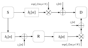
We consider the three-terminal model of an OFDM based AF relay system as shown in Fig. 1, which is composed of a source node S, a destination node D, and a relay node R. One transmission period is separated into two time slots. In the first time slot, S transmits an OFDM symbol of N subcarriers to R and D. In the second time slot, R amplifies and retransmits the OFDM symbol to D, where the corresponding gain factor is $\rho$. Further discussion about the gain factor $\rho$ is presented in Section III.

Figure 1: Baseband equivalent system model of an OFDM based AF relay system.

Let $X\left[k\right]$ denote the data symbol to be transmitted at source node S. Let $N_{g}$ denote the length of the cyclic prefix (CP). Then, with the application of inverse discrete Fourier transform (IDFT) to $X[k]$ and CP insertion, we have

$$x[n]=\frac{1}{N}\sum\limits_{k=0}^{N-1}{X[k]\exp[j2\pi k{{\left({n-N_{g}}\right)}\mathord{\left/{\vphantom{{\left({n-N_{g}}\right)}N}}\right.\kern-1.2pt}N}],}\$$ (1)

$${\rm{for}}\ 0\leq n\leq N+N_{g}-1.$$

In order to prevent possible inter-symbol interference (ISI) between OFDM symbols, we assume that $N_{g}\geq L_{1}$ and $N_{g}\geq L_{2}+L_{3}$, where $L_{1}$, $L_{2}$, $L_{3}$ are the delay spreads of the considered multipath channels $h_{1}[n]$, $h_{2}[n]$ and $h_{3}[n]$ as depicted in Fig. 1.

At destination node D, multiple CFOs will appear when the oscillator of D is not perfectly matched to the oscillators of S and R or there exists Doppler shift due to the mobility of D or R. Let $\varepsilon_{1}$ and $\varepsilon_{2}$ denote the frequency offsets of the direct link and relay link respectively, which are normalized by the OFDM subcarrier spacing. Define

$$c_{i}(\varepsilon_{i},n)\buildrel\Delta\over{=}\frac{1}{N}\exp({j2\pi\varepsilon_{i}n}\mathord{\left/{\vphantom{{j2\pi\varepsilon_{i}n}N}}\right.\kern-1.2pt}N),\ \mbox{for}\ i=1,2.$$

Then, the received signals of the direct link and relay link at destination node D can be expressed as

$$y_{1}[n]=Nc_{1}(\varepsilon_{1},n)(h_{1}[n]\ast x[n])+z_{1}[n],$$ (2)

$$y_{2}[n]=\rho Nc_{2}(\varepsilon_{2},n)(h_{2}[n]\ast h_{3}[n]\ast x[n])+\rho z_{{}_{2}}[n]+z_{3}[n],$$ (3)

where $z_{1}[n]$, $z_{2}[n]$ and $z_{3}[n]$ are AWGN with zero-mean and variance of $\sigma_{Z_{1}}^{2}$, $\sigma_{Z_{2}}^{2}$ and $\sigma_{Z_{3}}^{2}$, $\ast$ denotes the convolution operator, and the convolution operation of $x\left[n\right]$ and $y\left[n\right]$ is defined as $x\left[n\right]\ast y\left[n\right]=\sum\nolimits_{r=0}^{N-1}{x[r]y[n-r]}$ .

3 SNR Analysis

As we know, the CFO can be divided into an integer CFO (ICFO) and a fractional CFO (FCFO). The ICFO results in the cyclic shift of the subcarriers, and it should be corrected perfectly for the proper operation of the receiver. Thus, in the following, we only consider the effect of the FCFO on the SNR performance in OFDM based AF relay systems with the assumption that the ICFO has already been compensated.

Applying discrete Fourier transform (DFT) to $y_{1}[n]$ and $y_{2}[n]$, we have

$$Y_{1}\left[k\right] = C_{1}\left({\varepsilon_{1},k}\right)\ast(H_{1}\left[k\right]X\left[k\right])+Z_{1}\left[k\right]$$ (4)

$$= C_{1}\left({\varepsilon_{1},0}\right)H_{1}\left[k\right]X\left[k\right]+I_{1}\left[k\right]+Z_{1}\left[k\right],$$

$$Y_{2}[k] = \rho C_{2}(\varepsilon_{2},k)\ast(H_{2}[k]H_{3}[k]X[k])+\rho Z_{2}[k]+Z_{3}[k]$$ (5)

$$= \rho C_{2}\left(\varepsilon_{2},0\right)H_{2}\left[k\right]H_{3}\left[k\right]X\left[k\right]+\rho I_{2}\left[k\right]+\rho Z_{2}\left[k\right]$$

$$+Z_{3}\left[k\right],$$

where $H_{i}\left[k\right]$ and $Z_{i}\left[k\right]$ are the DFTs of $h_{i}[n]$ and $z_{i}[n]$ for $i=1,2,3$, $C_{i}\left({\varepsilon_{i},k}\right)$ is the DFT of $c_{i}(\varepsilon_{i},n)$ which can be expressed as

$$C_{i}(\varepsilon_{i},k)={\frac{\sin[\pi(\varepsilon_{i}-k)]}{N\sin[{\pi(\varepsilon_{i}-k)}\mathord{\left/{\vphantom{{\pi(\varepsilon_{i}-k)}N}}\right.\kern-1.2pt}N]}\exp\left[{j\pi\left({\varepsilon_{i}-k}\right)\left({1-\frac{1}{N}}\right)}\right]},$$

$$\mbox{for}\ i=1,2,$$

$I_{1}\left[k\right]$ and $I_{2}\left[k\right]$ are the inter-carrier interference (ICI) which can be expressed as

$$I_{1}\left[k\right]=\sum\limits_{r=1}^{N-1}{C_{1}\left({\varepsilon_{1},r}\right)H_{1}\left[{k-r}\right]X\left[{k-r}\right]},$$

$$I_{2}\left[k\right]=\sum\limits_{r=1}^{N-1}{C_{2}\left({\varepsilon_{2},r}\right)H_{2}\left[{k-r}\right]H_{3}\left[{k-r}\right]X\left[{k-r}\right]}.$$

A coherent receiver should be able to estimate the phase of $C_{1}\left({\varepsilon_{1},0}\right)H_{1}\left[k\right]$ and $C_{2}\left({\varepsilon_{2},0}\right)H_{2}\left[k\right]H_{3}\left[k\right]$ in order to decode the received signals correctly. Let

$$C_{1}\left({\varepsilon_{1},0}\right)H_{1}\left[k\right]=|C_{1}\left({\varepsilon_{1},0}\right)H_{1}\left[k\right]|\exp[{j\beta_{1}\left(k\right)}],$$

$$C_{2}\left({\varepsilon_{2},0}\right)H_{2}\left[k\right]H_{3}\left[k\right]$$

$$=|C_{2}\left({\varepsilon_{2},0}\right)H_{2}\left[k\right]H_{3}\left[k\right]|\exp[{j\beta_{2}\left(k\right)}].$$

Assume that $\beta_{1}\left(k\right)$ and $\beta_{2}\left(k\right)$ can be perfectly estimated, and define $R_{1}\left[k\right]=\exp[{-j\beta_{1}\left(k\right)}]Y_{1}\left[k\right]$, $R_{2}\left[k\right]=\exp[{-j\beta_{2}\left(k\right)}]Y_{2}\left[k\right]$. Then, we have

$$R_{1}\left[k\right]=|C_{1}\left({\varepsilon_{1},0}\right)H_{1}\left[k\right]|X\left[k\right]+I_{1}^{{}^{\prime}}\left[k\right]+Z_{1}^{{}^{\prime}}\left[k\right],$$ (6)

$$R_{2}\left[k\right]=\rho|C_{2}\left({\varepsilon_{2},0}\right)H_{2}\left[k\right]H_{3}\left[k\right]|X\left[k\right]+\rho I_{2}^{{}^{\prime}}\left[k\right]$$ (7)

$$+\rho Z_{2}^{{}^{\prime}}\left[k\right]+Z_{3}^{{}^{\prime}}\left[k\right],$$

where $Z_{1}^{{}^{\prime}}\left[k\right]=\exp\left[{-j\beta_{1}\left(k\right)}\right]Z_{1}\left[k\right]$, $Z_{2}^{{}^{\prime}}\left[k\right]=\exp\left[{-j\beta_{2}\left(k\right)}\right]$$Z_{2}\left[k\right]$, $Z_{3}^{{}^{\prime}}\left[k\right]=\exp\left[{-j\beta_{2}\left(k\right)}\right]Z_{3}\left[k\right]$, $I_{1}^{{}^{\prime}}\left[k\right]=\exp\left[{-j\beta_{1}\left(k\right)}\right]I_{1}\left[k\right]$, $I_{2}^{{}^{\prime}}\left[k\right]=\exp\left[{-j\beta_{2}\left(k\right)}\right]I_{2}\left[k\right]$. By employing equal gain combining (EGC), the decision metric $R[k]$ for coherent demodulation can be expressed as

$$R[k] = R_{1}[k]+R_{2}[k]$$ (8)

$$= \left({|C_{1}\left({\varepsilon_{1},0}\right)H_{1}\left[k\right]|+\rho|C_{2}\left({\varepsilon_{2},0}\right)H_{2}\left[k\right]H_{3}\left[k\right]|}\right)X\left[k\right]$$

$$+I_{1}^{{}^{\prime}}\left[k\right]+\rho I_{2}^{{}^{\prime}}\left[k\right]+Z_{1}^{{}^{\prime}}\left[k\right]+\rho Z_{2}^{{}^{\prime}}\left[k\right]+Z_{3}^{{}^{\prime}}\left[k\right].$$

Define the SNR at destination node D as follows

SNR (9)

$$={\mbox{E}\left\{{|\left({|C_{1}\left({\varepsilon_{1},0}\right)H_{1}\left(k\right)|\!+\!\rho|C_{2}\left({\varepsilon_{2},0}\right)H_{2}\left(k\right)H_{3}\left(k\right)|}\right)X\left(k\right)|^{2}}\right\}}$$

$$/\ {\mbox{E}\left[{|\left({I_{1}^{{}^{\prime}}\left[k\right]+\rho I_{2}^{{}^{\prime}}\left[k\right]+Z_{1}^{{}^{\prime}}\left[k\right]\!+\!\rho Z_{2}^{{}^{\prime}}\left[k\right]+Z_{3}^{{}^{\prime}}\left[k\right]}\right)|^{2}}\right]}.$$

Assume that all the considered channels are independent with each other and their means are zero. Let

$$\mbox{E}\left\{{|X[k]|^{2}}\right\}=\sigma_{X}^{2},\ \ \mbox{E}\left\{{|H_{i}[k]|^{2}}\right\}=\sigma_{H_{i}}^{2},\ \mbox{for}\ i=1,2,3.$$

Then, by exploiting the following relationship

$$\sum\limits_{r=0}^{N-1}{|C(\varepsilon_{i},r)|^{2}}=N\sum\limits_{r=0}^{N-1}{|c\left({\varepsilon_{i},r}\right)|^{2}}=1,\ \mbox{for}\ i=1,2,$$ (10)

the numerator and denominator of (9) can be simplified as follows

$$\mbox{E}\left\{{|\left({|C_{1}\left({\varepsilon_{1},0}\right)H_{1}\left(k\right)|+\rho|C_{2}\left({\varepsilon_{2},0}\right)H_{2}\left(k\right)H_{3}\left(k\right)|}\right)X\left(k\right)|^{2}}\right\}$$

$$= \mbox{E}\left[{|C_{1}\left({\varepsilon_{1},0}\right)|^{2}}\right]\sigma_{H_{1}}^{2}\sigma_{X}^{2}+\rho^{2}\mbox{E}\left[{|C_{2}\left({\varepsilon_{2},0}\right)|^{2}}\right]\sigma_{H_{2}}^{2}\sigma_{H_{3}}^{2}\sigma_{X}^{2},$$

$$\mbox{E}\left[{|\left({I_{1}^{{}^{\prime}}\left[k\right]+\rho I_{2}^{{}^{\prime}}\left[k\right]+Z_{1}^{{}^{\prime}}\left[k\right]+\rho Z_{2}^{{}^{\prime}}\left[k\right]+Z_{3}^{{}^{\prime}}\left[k\right]}\right)|^{2}}\right]$$

$$= \left\{{1-\mbox{E}\left[{|C_{1}\left({\varepsilon_{1},0}\right)|^{2}}\right]}\right\}\sigma_{{}_{H_{1}}}^{2}\sigma_{X}^{2}+\rho^{2}\left\{{1-\mbox{E}\left[{|C_{2}\left({\varepsilon_{2},0}\right)|^{2}}\right]}\right\}$$

$$\times\sigma_{{}_{H_{2}}}^{2}\sigma_{{}_{H_{3}}}^{2}\sigma_{X}^{2}+\sigma_{Z_{1}}^{2}+\rho^{2}\sigma_{Z_{2}}^{2}+\sigma_{Z_{3}}^{2}.$$

Accordingly, the SNR in (9) can be expressed as

SNR

$$={{\left\{\mbox{E}\left[{|C_{1}\left({\varepsilon_{1},0}\right)|^{2}}\right]\sigma_{H_{1}}^{2}\sigma_{X}^{2}+\rho^{2}\mbox{E}\left[{|C_{2}\left({\varepsilon_{2},0}\right)|^{2}}\right]\sigma_{H_{2}}^{2}\sigma_{H_{3}}^{2}\sigma_{X}^{2}\right\}}}$$

$$/\left\{\left\{{1-\mbox{E}\left[{|C_{1}\left({\varepsilon_{1},0}\right)|^{2}}\right]}\right\}\sigma_{{}_{H_{1}}}^{2}\sigma_{X}^{2}\right.$$

$$+\rho^{2}\left\{{1-\mbox{E}\left[{|C_{2}\left({\varepsilon_{2},0}\right)|^{2}}\right]}\right\}\sigma_{{}_{H_{2}}}^{2}\sigma_{{}_{H_{3}}}^{2}\sigma_{X}^{2}$$

$$\left.+\sigma_{Z_{1}}^{2}+\rho^{2}\sigma_{Z_{2}}^{2}+\sigma_{Z_{3}}^{2}\right\}.$$

For certain frequency offsets $\varepsilon_{1}$ and $\varepsilon_{2}$, the SNR can be further simplified as follows,

$$\mbox{SNR}\left({\varepsilon_{1},\varepsilon_{2}}\right)$$ (11)

$$=\left\{f_{N}^{2}\left({\varepsilon_{1}}\right)\sigma_{H_{1}}^{2}\sigma_{X}^{2}+\rho^{2}f_{N}^{2}\left({\varepsilon_{2}}\right)\sigma_{H_{2}}^{2}\sigma_{H_{3}}^{2}\sigma_{X}^{2}\right\}$$

$$/\left\{\left[{1-f_{N}^{2}\left({\varepsilon_{1}}\right)}\right]\sigma_{{}_{H_{1}}}^{2}\sigma_{X}^{2}+\rho^{2}\left[{1-f_{N}^{2}\left({\varepsilon_{2}}\right)}\right]\sigma_{{}_{H_{2}}}^{2}\sigma_{{}_{H_{3}}}^{2}\sigma_{X}^{2}\right.$$

$$\left.+\sigma_{Z_{1}}^{2}+\rho^{2}\sigma_{Z_{2}}^{2}+\sigma_{Z_{3}}^{2}\right\}$$

where $f_{N}\left({\varepsilon_{i}}\right)={\sin\left({\pi\varepsilon_{i}}\right)}/\left[N\sin\left({\pi\varepsilon_{i}/N}\right)\right]$ for $i=1,2$. From (11), it is obvious that the existence of multiple CFOs introduces SNR degradation, and it can be seen that the SNR decreases as the CFO $\varepsilon_{1}$ or $\varepsilon_{2}$ increases from 0 to 1/2 and that it is maximized if and only if $\varepsilon_{1}=\varepsilon_{2}=0$.

Define the sensitivities of the SNR to $\varepsilon_{1}$ and $\varepsilon_{2}$ as follows

$$\lambda_{1}=|\frac{\partial\mbox{SNR}\left({\varepsilon_{1},\varepsilon_{2}}\right)}{\partial\varepsilon_{1}}|,\ \lambda_{2}=|\frac{\partial\mbox{SNR}\left({\varepsilon_{1},\varepsilon_{2}}\right)}{\partial\varepsilon_{2}}|.$$ (12)

Then, we have

$$\lambda_{1} = \frac{2|f_{N}^{{}^{\prime}}(\varepsilon_{1})|\sigma_{H_{1}}^{2}\sigma_{X}^{2}(A+B)}{B^{2}},\$$

$$\lambda_{2} = \frac{2|f_{N}^{{}^{\prime}}(\varepsilon_{2})|\rho^{2}\sigma_{H_{2}}^{2}\sigma_{H_{3}}^{2}\sigma_{X}^{2}(A+B)}{B^{2}},$$ (13)

where A and B are the numerator and denominator of (11), respectively. By comparing $\lambda_{1}$ with $\lambda_{2}$ in (3), it can be seen that the sensitivities of the SNR to $\varepsilon_{1}$ and $\varepsilon_{2}$ are different. The difference is mainly caused by the different power of the corresponding link channel and gain factor.

As far as the gain factor $\rho$ is concerned, it can be expressed as

$$\rho=\sqrt{\frac{P_{R}}{\sigma_{H_{2}}^{2}P_{S}+\sigma_{Z_{2}}^{2}}},$$ (14)

where $P_{R}$ and $P_{S}$ are the average transmitting power of R and S, respectively. Under the power constraint $P=P_{S}+P_{R}$, many power allocation (PA) schemes can be applied. Basically, they can be classified as uniform power allocation (UPA) and optimal power allocation (OPA). In the following, unless otherwise stated, UPA is adopted. Nevertheless, it can be easily extended to OPA. Employing UPA, we obtain

$$\rho=\sqrt{\frac{1}{\sigma_{H_{2}}^{2}+{2\sigma_{Z_{2}}^{2}}/{P}}}.$$ (15)

When $P\gg\sigma_{z_{2}}^{2}$, we have $\rho\approx{1\mathord{\left/{\vphantom{1{\sqrt{\sigma_{H_{2}}^{2}}}}}\right.\kern-1.2pt}{\sqrt{\sigma_{H_{2}}^{2}}}}$. By employing the above simplification, (11) and (3) can be rewritten as follows

$$\mbox{SNR}\left({\varepsilon_{1},\varepsilon_{2}}\right)$$ (16)

$$=\left\{f_{N}^{2}\left({\varepsilon_{1}}\right)\sigma_{H_{1}}^{2}\sigma_{X}^{2}+f_{N}^{2}\left({\varepsilon_{2}}\right)\sigma_{H_{3}}^{2}\sigma_{X}^{2}\right\}$$

$$/\left\{\left[{1-f_{N}^{2}\left({\varepsilon_{1}}\right)}\right]\sigma_{{H_{1}}}^{2}\sigma_{X}^{2}+\left[{1-f_{N}^{2}\left({\varepsilon_{2}}\right)}\right]\sigma_{{H_{3}}}^{2}\sigma_{X}^{2}\right.$$

$$\left.+\sigma_{Z_{1}}^{2}+\sigma_{H_{2}}^{2}\sigma_{Z_{2}}^{2}+\sigma_{Z_{3}}^{2}\right\},$$

$$\lambda_{1} = \frac{2|f_{N}^{{}^{\prime}}(\varepsilon_{1})|\sigma_{H_{1}}^{2}\sigma_{X}^{2}(A+B)}{B^{2}},$$

$$\lambda_{2} = \frac{2|f_{N}^{{}^{\prime}}(\varepsilon_{2})|\sigma_{H_{3}}^{2}\sigma_{X}^{2}(A+B)}{B^{2}}.$$ (17)

From (3), it can be seen that the sensitivity of the SNR to $\varepsilon_{1}$ and $\varepsilon_{2}$ is determined only by the power of the direct link channel and that of the second hop of the relay link channel when UPA is employed.

Furthermore, according to the above analysis, we can easily extend the SNR expression in (11) to the multiple-relay-node scenario as depicted in Fig. 2 as follows

$$\mbox{SNR}\left({\varepsilon_{0},\varepsilon_{1},...,\varepsilon_{M}}\right)$$ (18)

$$=\left\{f_{N}^{2}\left({\varepsilon_{0}}\right)\sigma_{H_{0}}^{2}\sigma_{X}^{2}+\sum\limits_{i=1}^{M}{\rho_{i}^{2}f_{N}^{2}\left({\varepsilon_{i}}\right)\sigma_{H_{i1}}^{2}\sigma_{H_{i2}}^{2}}\sigma_{X}^{2}\right\}$$

$$/\left\{\left[{1-f_{N}^{2}\left({\varepsilon_{0}}\right)}\right]\sigma_{{}_{H_{0}}}^{2}\sigma_{X}^{2}+\sum\limits_{i=1}^{M}{\rho_{i}^{2}\left[{1-f_{N}^{2}\left({\varepsilon_{i}}\right)}\right]\sigma_{{}_{H_{i1}}}^{2}\sigma_{{}_{H_{i2}}}^{2}}\sigma_{X}^{2}\right.$$

$$\left.+\sigma_{Z_{0}}^{2}+\sum\limits_{i=1}^{M}{\left({\sigma_{Z_{i1}}^{2}+\rho_{i}^{2}\sigma_{Z_{i2}}^{2}}\right)}\right\}.$$

4 Simulation Results

In this section, simulation results are given to verify the analytical results under the following conditions: $\sigma_{z_{1}}^{2}=\sigma_{z_{2}}^{2}=\sigma_{z_{3}}^{2}$ and $\sigma_{H_{3}}^{2}=4\sigma_{H_{1}}^{2}$.

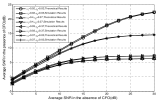
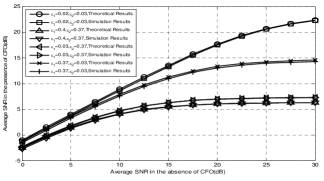
Fig. 3 presents the average SNR in the presence of CFO for flat fading channels, while Fig. 4 shows the average SNR in the presence of CFO for frequency-selective fading channels. It can be seen that the simulation results and theoretical results match very well. When the CFOs increase, the SNR decreases dramatically. The SNR is more sensitive to $\varepsilon_{2}$, and the SNR degradation due to the CFOs is more serious in the high SNR region. Compared with the flat fading channel, the frequency-selective fading channel shows slightly larger SNR degradation.

5 Conclusions

In this letter, we have analyzed the effect of the CFOs on OFDM based AF relay systems. From the derived SNR expression, it has been found that the SNR decreases monotonically as the frequency offsets increase. Both analytical and numerical results have shown that the SNR degradation due to the CFOs at high SNR values is larger than that at low SNR values and that the sensitivity of the SNR to CFO is mainly determined by the power of the corresponding link channel and gain factor.

Figure 2: The Schematic of a multiple-relay-node AF system.

Figure 3: Average SNR in the presence of CFO for flat fading channels.

Figure 4: Average SNR in the presence of CFO for frequency-selective fading channels.

References

• [1] J. A. C. Bingham, “Multicarrier modulation for data transmission:an idea whose time has come,” IEEE Commun. Mag., vol. 28, pp. 5–14, May 1990.
• [2] R. Pabst, B. H. Walke, and D. C. Schultz, “Relay-based deployment concepts for wireless and mobile broadband radio,” IEEE Commun. Mag., vol. 42, no. 9, pp. 80–88, Sept. 2004.
• [3] M. Herdin, “A chunk based OFDM amplify-and-forward relaying scheme for 4G mobile radio systems,” in Proc. IEEE ICC’06, vol. 10, June 2006, pp. 4507–4512.
• [4] C. K. Ho and A. Pandharipande, “BER minimization in relay-assisted OFDM systems by subcarrier permutation,” in Proc. IEEE VTC’08 Spring, May 2008, pp. 1489–1493.
• [5] M. Kaneko, K. Hayashi, P. Popovski, and et al., “Amplify-and-forward cooperative diversity schemes for multi ccarrier systems,” IEEE Trans. Wireless Commun., vol. 7, no. 5, pp. 1845–1850, May 2008.
• [6] T. Pollet, M. V. Bladel, and M. Moeneclaey, “BER sensitivity of OFDM systems to carrier frequency offset and Wiener phase noise,” IEEE Trans. Commun., vol. 43, pp. 191–193, Feb./Mar./Apr. 1995.
• [7] H. Nikookar and R. Prasad, “On the sensitivity of multicarrier transmission over multipath channels to phase noise and frequency offsets,” in Proc. IEEE PIMRC’96, 1996, pp. 68–72.
• [8] W. Hwang, H. Kang, and K. Kim, “Approximation of SNR degradation due to carrier frequency offset for OFDM in shadowed multipath channels,” IEEE Commun. Lett., vol. 7, no. 12, pp. 581–583, Dec. 2003.
• [9] X. Ma, H. Kobayashi, and S. C. Schwartz, “Effect of frequency offset on BER of OFDM and single carrier systems,” in Proc. IEEE PIMRC’03, 2003, pp. 2239–2243.
Refer to caption