libvdwxc: A library for exchange–correlation functionals in the vdW-DF family

Abstract

We present libvdwxc, a general library for evaluating the energy and potential for the family of vdW-DF exchange–correlation functionals. libvdwxc is written in C and provides an efficient implementation of the vdW-DF method and can be interfaced with various general-purpose DFT codes. Currently, the Gpaw and Octopus codes implement interfaces to libvdwxc. The present implementation emphasizes scalability and parallel performance, and thereby enables ab initio calculations of nanometer-scale complexes. The numerical accuracy is benchmarked on the S22 test set whereas parallel performance is benchmarked on ligand-protected gold nanoparticles ($\text{Au}_{144}(\text{SC}_{11}\text{NH}_{25})_{60}$) up to 9696 atoms.

1 Introduction

Kohn–Sham density functional theory [1, 2] (DFT) is widely used as a predictive tool in areas ranging from chemistry and materials physics to biochemical applications. The continually increasing computational power is pushing the reach of ab initio modelling to the nanometer scale and provides access to systems with remarkable diversity. Many of these are sufficiently sparse in terms of the spatial distribution of the electron density for dispersive interactions to play a role [3]. In addition to requiring extensive computational resources, the common denominator among these systems is the importance of van der Waals (vdW) interactions.

This situation has prompted the development of the vdW density functional (vdW-DF) method [4, 5] which comprises a growing family of exchange–correlation (XC) functionals. These include vdW-DF1 [6, 7], vdW-DF2 [8], vdW-DF-C09 [9], vdW-DF-cx [10], vdW-DF-optb86 [11], rev-vdW-DF2 [12], vdW-DF-optPBE, vdW-DF-optB88 [13], BEEF-vdW [14], and mBEEF-vdW [15]. In those functionals the nonlocal correlation forces are captured through a formal analysis of screened response in the electron gas [4]. Closely related is also VV10 [16] and revised VV10 [17], which adapt the vdW-DF framework to a simpler response description. The vdW-DF method can characterize both pure vdW forces and vdW forces in combination with other types of binding [18, 4]. The vdW-DF method has gained a reputation for providing accurate characterizations and predictions for a range of systems including but not limited to metals [13, 19], layered materials [20, 21, 22, 18, 23], and molecular systems [10, 24, 25, 26, 27].

In the vdW-DF family, the XC energy can be written in the form

$$E_{\text{xc}}[n] =E_{\text{x}}^{\text{GGA}}[n]+E_{\text{c}}^{\text{LDA}}[n]+E_{\text{c}}^{\text{nl}}[n].$$ (1)

Here, $E_{\text{x}}^{\text{GGA}}[n]$ is an exchange energy functional in the generalized gradient approximation (GGA), and $E_{\text{c}}^{\text{LDA}}[n]$ is the well-established Perdew–Wang parametrization of the correlation energy in the local-density approximation (LDA) [28]. The third term is the characteristic non-local correlation energy functional of the vdW-DF method that describes the vdW interactions,

$$E_{\mathrm{c}}^{\text{nl}}[n] =\frac{1}{2}\iint n(\boldsymbol{\mathrm{r}})\phi\big{(}q_{0}(\boldsymbol{\mathrm{r}}),q_{0}(\boldsymbol{\mathrm{r}}^{\prime}),|\boldsymbol{\mathrm{r}}-\boldsymbol{\mathrm{r}}^{\prime}|\big{)}n(\boldsymbol{\mathrm{r}}^{\prime})\,\mathrm{d}\boldsymbol{\mathrm{r}}\,\mathrm{d}\boldsymbol{\mathrm{r}}^{\prime},$$ (2)

which has a different formal structure from semilocal functionals. In (2), $\phi(q_{0},q_{0}^{\prime},r)$ is the vdW kernel, and $q_{0}(\boldsymbol{\mathrm{r}})$ represents an inverse length scale that characterizes the roll-over in the vdW-DF plasmon-pole description. This roll-over function $q_{0}(\boldsymbol{\mathrm{r}})$ is determined by the energy per particle of an internal GGA-type functional [8, 29, 4], and is therefore local, depending exclusively on the local density and its gradient.

The integral (2) is six-dimensional, but it can be efficiently computed using a spline decomposition of the two spatial variables together with the Fourier convolution theorem [30].

While the vdW-DF method has been implemented, e.g., in the Siesta [31], Abinit [32], Quantum Espresso [33], Vasp [34], and Gpaw [35] codes, both performance and results vary. Typical vdW forces are small, corresponding to shallow potential energy landscapes with weak curvature. Bonding distances are sensitive to even small differences in implementations. Hence a standardized reference implementation is of great interest.

We therefore present here the libvdwxc software library that provides an efficient implementation of the vdW-DF method and can be interfaced with various general-purpose DFT codes.

What libvdwxc does is to compute the non-local correlation energy (2) and its derivatives for evaluating the potential. The corresponding semilocal functionals in (1) are available from the libxc library [38]. Indeed the success of libxc has been a major source of inspiration for libvdwxc. libvdwxc complements libxc so that all the functionals in the vdW-DF family mentioned above are accessible given the two libraries. The reason why libvdwxc is a separate library and not part of libxc is the big difference between semilocal and fully non-local functionals. libxc relies on the fact that all the supported functionals are evaluated pointwise: At each point, the calculation requires only the density and its derivatives in that point. Since the vdW-DF functionals are non-local, libvdwxc must instead work on the full density. The evaluation also requires separate array allocations and fast Fourier transforms (FFTs), and is non-trivial to parallelize. libvdwxc therefore depends on FFTs from the FFTW library [39] or optionally PFFT [40]. Parallelism is supported through MPI.

libvdwxc does not at present include other vdW-inclusive approaches such as the Wannier function approach [41, 42], the Tkatchenko–Scheffler method [43], the Grimme D-correction series [44, 45], or exchange-hole dipole moment theory [46].

The remainder of this article is organized as follows. In the following section, we review the Román-Pérez–Soler algorithm. (Background information concerning construction and interpretation of the vdW-DF method can be found in Refs. [4] and [29]). Section 3 is a detailed description of the parallel implementation of vdW-DF. Calculated results are benchmarked against other codes in Section 4. We demonstrate the excellent scalability of the library in Section 5. Finally, a brief technical description is provided in Section 6.

2 Román-Pérez–Soler method

While Eq. (2) is prohibitively expensive to evaluate by direct numerical integration in six dimensions , it can be efficiently approximated by the 2D interpolation method by Román-Pérez and Soler [30]. The idea is to replace the continuous $q_{0}$ parameters of the kernel $\phi(q_{0},q_{0}^{\prime},r)$ by a grid of $M$ discrete $q_{0}$ values, such that the kernel is instead described by $M\times M$ radial functions $\phi_{\alpha\beta}(r)$ with $\alpha,\beta=0,1,\ldots,M-1$. A spline representation over the $q_{0}$ grid is used to retain high numerical precision between the points of the discrete $q_{0}$ grid [30]. Specifically this is done by introducing $M$ helper splines $p_{\alpha}(q_{0})$ such that $p_{\alpha}(q_{0}^{\beta})=\delta_{\alpha\beta}$: Each function takes the value 1 on its “own” mesh point and 0 on all the others. Between the mesh points the functions oscillate weakly. The spline representation interpolates both $q_{0}$ and $q_{0}^{\prime}$ of $\phi(q_{0},q_{0}^{\prime},r)$, combining to produce an overall accurate and smooth representation over the whole range of $(q_{0},q_{0}^{\prime})$. The full definition of the helper function $p_{\alpha}(q_{0})$ at the grid point $q_{0}^{\beta}$ plus a small displacement $\mathrm{d}q_{0}$ is

$$p_{\alpha}(q_{0}^{\beta}+\mathrm{d}q_{0})=\sum_{c=0}^{3}a^{c}_{\alpha\beta}(\mathrm{d}q_{0})^{c},0\leq{\mathrm{d}q_{0}}<q_{0}^{\beta+1}-q_{0}^{\beta}.$$ (3)

The coefficients $a_{\alpha\beta}$ are determined by the aforementioned condition that $p_{\alpha}(q_{0}^{\beta})=\delta_{\alpha\beta}$, along with the requirement of continuity of derivatives up to second order. It was found in Ref. [30] that $M=20$ mesh points were sufficient to achieve good precision. This remains the standard procedure today, although a smoother representation of the kernel has recently been suggested which reduces the required number of points [48].

We now define the auxiliary quantity

$$\theta_{\alpha}(\boldsymbol{\mathrm{r}})=n(\boldsymbol{\mathrm{r}})p_{\alpha}(q_{0}(\boldsymbol{\mathrm{r}})),$$ (4)

which is the key quantity in actual computations. The energy can then be written as

$$E_{\mathrm{c}}^{\text{nl}}[n] =\frac{1}{2}\sum_{\alpha\beta}\iint\theta_{\alpha}(\boldsymbol{\mathrm{r}})\phi_{\alpha\beta}(|\boldsymbol{\mathrm{r}}^{\prime}-\boldsymbol{\mathrm{r}}|)\theta_{\beta}(\boldsymbol{\mathrm{r}}^{\prime})\,\mathrm{d}\boldsymbol{\mathrm{r}}^{\prime}\,\mathrm{d}\boldsymbol{\mathrm{r}}$$

$$=\frac{1}{2}\sum_{\alpha}\int\theta_{\alpha}(\boldsymbol{\mathrm{r}})F_{\alpha}(\boldsymbol{\mathrm{r}})\,\mathrm{d}\boldsymbol{\mathrm{r}},$$ (5)

where

$$F_{\alpha}(\boldsymbol{\mathrm{r}})=\sum_{\beta}\int\phi_{\alpha\beta}(|\boldsymbol{\mathrm{r}}-\boldsymbol{\mathrm{r}}^{\prime}|)\theta_{\beta}(\boldsymbol{\mathrm{r}}^{\prime})\,\mathrm{d}\boldsymbol{\mathrm{r}}^{\prime}.$$ (6)

This integral is a convolution, and the energy can therefore be written using the convolution theorem as

$$E_{\mathrm{c}}^{\text{nl}}[n]=\frac{1}{2}\sum_{\alpha\beta}\int\theta^{*}_{\alpha}(\boldsymbol{\mathrm{k}})\phi_{\alpha\beta}(k)\theta_{\beta}(\boldsymbol{\mathrm{k}})\,\mathrm{d}\boldsymbol{\mathrm{k}},$$ (7)

where $\theta_{\alpha}(\boldsymbol{\mathrm{k}})$ is the Fourier transform of $\theta_{\alpha}(\boldsymbol{\mathrm{r}})$.

Practical calculations also require the potential, which is defined as the derivative of the energy with respect to the density,

$$v_{\mathrm{c}}^{\text{nl}}(\boldsymbol{\mathrm{r}})\equiv\frac{\delta E_{\mathrm{c}}^{\text{nl}}[n]}{\delta n(\boldsymbol{\mathrm{r}})}=\left.\frac{\partial E_{\mathrm{c}}^{\text{nl}}[n]}{\partial n(\boldsymbol{\mathrm{r}})}\right|_{\sigma}+\left.\frac{\partial E_{\mathrm{c}}^{\text{nl}}[n]}{\partial\sigma(\boldsymbol{\mathrm{r}})}\right|_{n}\frac{\mathrm{d}\sigma(\boldsymbol{\mathrm{r}})}{\mathrm{d}n(\boldsymbol{\mathrm{r}})},$$ (8)

where $\sigma(\boldsymbol{\mathrm{r}})=|\boldsymbol{\mathrm{\nabla}}n(\boldsymbol{\mathrm{r}})|^{2}$. The partial derivatives are

$$\frac{\partial E_{\mathrm{c}}^{\text{nl}}[n]}{\partial n(\boldsymbol{\mathrm{r}})} =\sum_{\alpha}F_{\alpha}(\boldsymbol{\mathrm{r}})\left[p_{\alpha}(q_{0}(\boldsymbol{\mathrm{r}}))+n(\boldsymbol{\mathrm{r}})p_{\alpha}^{\prime}(q_{0}(\boldsymbol{\mathrm{r}}))\frac{\partial q_{0}(\boldsymbol{\mathrm{r}})}{\partial n(\boldsymbol{\mathrm{r}})}\right],$$ (9)

$$\frac{\partial E_{\mathrm{c}}^{\text{nl}}[n]}{\partial\sigma(\boldsymbol{\mathrm{r}})} =n(\boldsymbol{\mathrm{r}})\sum_{\alpha}F_{\alpha}(\boldsymbol{\mathrm{r}})\frac{\mathrm{d}p_{\alpha}(q_{0}(\boldsymbol{\mathrm{r}}))}{\mathrm{d}q_{0}(\boldsymbol{\mathrm{r}})}\frac{\partial q_{0}(\boldsymbol{\mathrm{r}})}{\partial\sigma(\boldsymbol{\mathrm{r}})}.$$ (10)

libvdwxc implements these partial derivatives, while the calling DFT code is responsible for calculating the density-derivative $\sigma(\boldsymbol{\mathrm{r}})$ and combining the calculated partial derivatives (9) and (10) to obtain the potential. Any DFT code that supports GGAs already implements the requisite functionality, which is also the requirement for calling libxc. For completeness we provide the expression for $q_{0}(\boldsymbol{\mathrm{r}})$ in the appendix (see also Ref. [6]).

libvdwxc currently uses the standard kernel and mesh representation from Quantum Espresso. This means using the same 20 mesh points $q_{0}^{\alpha}$ and the same $20\times 20$ radial functions $\phi_{\alpha\beta}(k)$; Support for multiple pluggable kernels (e.g. the GPAW parametrization) is under development.

3 Computation and parallelization

Expression	Description	Scaling	Expensive
$q_{0}\big{(}n(\boldsymbol{\mathrm{r}}),\sigma(\boldsymbol{\mathrm{r}})\big{)}$	math	$\mathcal{O}(N)$	no
$\theta_{\alpha}(\boldsymbol{\mathrm{r}})$	splines	$\mathcal{O}(N)$	no
$\theta_{\alpha}(\boldsymbol{\mathrm{k}})$	20 $\times$ FFT	$\mathcal{O}(N\log N)$	yes
$E_{\mathrm{c}}^{\text{nl}}$, $F_{\alpha}(\boldsymbol{\mathrm{k}})$	400 integrals	$\mathcal{O}(N)$	yes
$F_{\alpha}(\boldsymbol{\mathrm{r}})$	20 $\times$ iFFT	$\mathcal{O}(N\log N)$	yes
$v_{\mathrm{c}}^{\text{nl}}(\boldsymbol{\mathrm{r}})$	math	$\mathcal{O}(N)$	no

Table 1: Steps in a vdW calculation and their computational scaling with respect to the total number $N$ of real-space points.

vdW calculations are significantly more complex than ordinary GGA calculations. The calculation needs to allocate at least 20 functions ($\theta_{\alpha}(\boldsymbol{\mathrm{r}})$) on top of a GGA calculation. Furthermore, vdW systems are often very sparse, and due to the long range of the vdW interactions, a larger vacuum region is often required to avoid artificial interactions between periodic images. Good performance is therefore important and in particular good parallel scalability. The computational complexity of a vdW calculation is $\mathcal{O}(N\log N)$ due to the Fourier transforms, whereas standard Kohn–Sham DFT scales as $\mathcal{O}(N^{3})$. Therefore the vdW calculation will hardly topple the computational budget for large systems unless it is grossly unscalable. Since part of the reason to write libvdwxc is to provide a scalable implementation, we discuss the technical aspects in some detail below.

The calculation of vdW energy and potential involves the steps listed in Table 1. The computationally important parts of the calculation are the Fourier transforms, and to a lesser extent the convolution in Fourier space for calculating $F_{\alpha}(\boldsymbol{\mathrm{k}})$ and the energy.

The ($\alpha$, $\boldsymbol{\mathrm{r}}$) and ($\alpha$, $\boldsymbol{\mathrm{k}}$) arrays can be distributed over $\alpha$ or $\boldsymbol{\mathrm{r}}/\boldsymbol{\mathrm{k}}$. Parallelization over $\alpha$ is not overly promising, though, as there are only $M=20$ of them. libvdwxc therefore distributes $\theta_{\alpha}(\boldsymbol{\mathrm{r}})$ over $\boldsymbol{\mathrm{r}}$ and, taking advantage of the parallel features of FFTW, correspondingly distributes $\theta_{\alpha}(\boldsymbol{\mathrm{k}})$ over $\boldsymbol{\mathrm{k}}$. We have found this type of parallelization to be quite sufficient (see Section 5), and so have not implemented simultaneous parallelization over $\alpha$.

libvdwxc assumes that the electron density is provided on a uniform real-space grid within a simulation cell that is a parallelepiped. This means $\theta_{\alpha}(\boldsymbol{\mathrm{k}})$ is calculated from 20 standard 3D FFTs of the real-valued functions $\theta_{\alpha}(\boldsymbol{\mathrm{r}})$. A 3D FFT on a $p\times q\times r$ grid consists of many 1D FFTs: First $p\times q$ FFTs of length $r$ over the $z$ axis, then likewise over $y$ and $x$. Distributing the many 1D FFTs over many cores is more efficient than performing inherently parallel 1D FFTs. In FFTW the data is initially distributed along the $x$ (least memory-contiguous) axis. The FFTs over $z$ and $y$ can be performed immediately, but then the data must be redistributed using a parallel transpose to allow the FFT over $x$. This is handled by FFTW, but the initial data distribution must still be set up by the caller.

Codes that wish to interface with libvdwxc must therefore redistribute their density to the initial FFTW-MPI layout: Process $n$ is responsible for $B$ elements along the $x$ axis numbered $nB$ to $(n+1)B$ (truncated if necessary to total number of points), where the blocksize $B$ should divide all the points between all available cores as evenly as possible. Implementing this redistribution is the most complex task from the perspective of the calling DFT code, although many codes may already support this feature if they employ parallel FFTs (e.g. Octopus [49]).

The distribution takes advantage of as many cores as there are grid points along the coordinate axes. If more cores are available, they will be idle during this stage. This does not occur in normal calculations, but is insufficient for massively parallel architectures. For this case libvdwxc can use PFFT [40], which relies on FFTW while extending parallelization to two dimensions (PFFT in general supports parallelization over $n-1$ dimensions for an $n$-dimensional Fourier transform). This is much more scalable, but requires another parallel transpose between the transforms over $z$ and $y$. For common forms of parallelism we therefore recommend standard FFTW with MPI.

The full calculation procedure is:

1. Evaluate the functions $\theta_{\alpha}(\boldsymbol{\mathrm{r}})$ as an array $\bar{\theta}_{xyz\alpha}$ distributed over $x$. Here and below, bars “$\bar{\ }$” denote arrays indexed by one or more subscripted quantities. The rightmost subscripted quantity (in this case $\alpha$) is contiguous in memory.

2. Compute the FFT of $\bar{\theta}_{xyz\alpha}$ in-place (input and output buffers are the same). This yields $\bar{\theta}_{k_{x}k_{y}k_{z}\alpha}$, now distributed over $k_{y}$.

3. For each $\boldsymbol{\mathrm{k}}=(k_{x},k_{y},k_{z})$, processing only the local $k_{y}$ for each process:

   1. Compute the kernel as an $M\times M$ matrix $\bar{\phi}^{k}_{\alpha\beta}$ using linear interpolation to resolve the kernel function values for the continuous variable $k$ from the discrete $k$-grid on which they are represented.

   2. Calculate $F_{\alpha}(\boldsymbol{\mathrm{k}})$ as the matrix–vector product

      $$\bar{F}_{\alpha}^{\boldsymbol{\mathrm{k}}}=\sum_{\beta}\bar{\phi}^{k}_{\alpha\beta}\bar{\theta}_{k_{x}k_{y}k_{z}\beta}.$$ (11)

      $\bar{F}_{\alpha}^{\boldsymbol{\mathrm{k}}}$ is a buffer of size $M$.

   3. Sum up the energy contributions

      $$\Delta E_{\mathrm{c}}^{\text{nl}}=\sum_{\alpha}\bar{\theta}_{k_{x}k_{y}k_{z}\alpha}^{*}\bar{F}_{\alpha}^{\boldsymbol{\mathrm{k}}},$$ (12)

      and write the buffer $\bar{F}_{\alpha}^{\boldsymbol{\mathrm{k}}}$ back into the same buffer as $\bar{\theta}_{k_{x}k_{y}k_{z}\alpha}$, now denoted $\bar{F}_{k_{x}k_{y}k_{z}\alpha}$.

4. Compute the inverse in-place FFT of $\bar{F}_{k_{x}k_{y}k_{z}\alpha}$ to obtain $\bar{F}_{xyz\alpha}$, once again distributed over $x$.

5. Compute the energy-derivatives using (9) and (10).

The above procedure follows the efficiency recommendations of FFTW:

1. The memory layout of the input buffer is strided, so for each point $\boldsymbol{\mathrm{r}}$ of space, values for the $M=20$ different $\alpha$ are stored contiguously rather than the other way around,

2. the transform is performed in-place, and

3. the output array remains in its transposed form, i.e., it is distributed over the second axis instead of the first.

We note that only a single work buffer is used for the four quantities $\theta_{\alpha}(\boldsymbol{\mathrm{r}})$, $\theta_{\alpha}(\boldsymbol{\mathrm{k}})$, $F_{\alpha}(\boldsymbol{\mathrm{k}})$, and $F_{\alpha}(\boldsymbol{\mathrm{r}})$. libvdwxc allocates memory for 23 spatial functions: $M=20$ for the workbuffer, plus $q_{0}$ and its two partial derivatives.

4 Numerical benchmarks

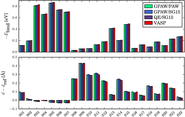
Figure 1: Benchmark of S22 dataset for different implementations of vdW-DF-cx. Binding energy (top) and equilibrium bond length (bottom) calculated using: Gpaw with libvdwxc and PBE PAW datasets (green); Gpaw with libvdwxc and the norm-conserving SG15 pseudopotentials (blue); QE (purple) and Vasp (red) codes using their internal vdW implementations.

To establish the numerical accuracy of libvdwxc, the current implementation is here benchmarked using Gpaw [35, 50], comparing to Quantum Espresso [33] (QE) and Vasp [34, 51]. To this end, we consider the standard S22 test set for dispersive interactions [52] and use the vdW-DF-cx functional [10]. Each member of the S22 test set corresponds to a weakly bound pair of small molecules at different intermolecular distances. The calculated total energies therefore yield an intermolecular binding curve.

All calculations are carried out using PAW setups or pseudopotentials for the PBE functional. Energies are evaluated for a series of distances $d_{i}=d_{\mathrm{ref}}+i\cdot 0.025$ Å, where $d_{\mathrm{ref}}$ is the reference equilibrium distance [52] for that S22 member; binding energies and distances are then fitted from the 5 values of $i$ that surround the calculated minimum. The simulation cell is such that no atom would be closer to any edge than $10$ Å at intermolecular separation $d^{\mathrm{ref}}+5$ Å. For each S22 member, the full series uses the same simulation cell.

For each separation $d_{i}$, the binding energy $E[AB]-E[A]-E[B]$ is evaluated by performing the calculations for each isolated molecule $A$ and $B$ with the atoms kept at the same absolute positions as in the dimer calculation $AB$. The purpose of this is to minimize the egg-box effect.

Gpaw calculations use real-space (FD) mode with the the standard PAW datasets (version 0.9.11271) and grid spacing 0.14 Å, as well as the norm-conserving SG15 pseudopotentials [53] with grid spacing 0.1 Å. The calculations use the FFT Poisson solver.

QE calculations use the norm-conserving SG15 pseudopotentials with a planewave cutoff of 1800 eV, while VASP calculations use the standard PAW datasets and a cutoff of 680 eV.

Figure 1 shows the results: The codes produce progressively stronger binding energies in the order Gpaw/PAW (weakest binding), Gpaw/SG15 (+1.4 meV on average with respect to Gpaw/GPAW), QE (+3.8 meV), and Vasp (+6.2 meV), and as binding energies become stronger, equilibrium bond lengths usually become smaller (on average 0, -0.92, -5.51, and -6.76, respectively, times $10^{-3}$ Å).

All these methods yield slightly different results, but no single method is in strong disagreement compared to the rest. Comparing Gpaw/PAW and Gpaw/SG15, the main difference is the representation of the atoms. Between Gpaw/SG15 and QE, the main difference is real-space versus planewave representation, although there are clearly many other implementation differences. Finally Vasp again uses PAW and has its own vdW-DF kernel.

Aside from the differences in atomic representation itself, the Gpaw/PAW and Gpaw/SG15 calculations have a more profound reason to differ: (1) the vdW-DF implementation in GPAW does not take into account that the PAW datasets are not norm-conserving, and (2) the calculations lack PAW corrections for non-local XC contributions because the standard equations are derived for semilocal functionals [54].

To elaborate on point (1), when the states are not norm-conserving, the contribution from each state to the valence electron density does not integrate exactly to one electron. As a result, the total pseudodensity from which the XC energy is evaluated is “deficient”, and the PAW corrections only compensate for this in the semilocal terms. This must be assumed to spuriously affect the non-local energy. For the chemical species included in the S22 test set, the particular PAW datasets used by Gpaw are, however, rather close to norm-conserving. The s and p valence states of H, B, C, N, and O have norms between 0.88 and 1.07. This may explain that the error is small and does not cause a clear discrepancy.

The regions far away from the atoms are also likely to provide most of the contribution to the bonding [55, 56, 10, 29]. In these regions the density is equal to the true (all-electron) density, and the errors mentioned do not apply. This is another reason why the errors may be (almost) neglected. Overall, the error associated with the use of PAW without non-local XC corrections for lack of norm-conservation is therefore not much larger than the implementation error present between different codes. Note, however, that this conclusion applies only to molecules similar to those in the S22 set. In particular the situation is different for metals, for which the PAW norm is often only around 0.3 electrons per d state.

In conclusion, 1) while the different methods and codes produce different results, there are no gross outliers; and 2) the neglection of PAW corrections has not caused the PAW calculations to particularly disagree with pseudopotential calculations.

5 Performance

The Román-Pérez–Soler algorithm solves the fundamental serial performance issue of vdW functionals, but parallel scalability remains essential for modern parallel computation. In this section we investigate the scalability of libvdwxc for large systems using the DFT code Gpaw [35, 50] in the ASE framework [57].

We consider a system of 2424 atoms: An Au₁₄₄ nanoparticle protected by 60 extended thiol ligands [58] (SC₁₁NH₂₅) as shown in Fig. 2. The system is chosen for its prodigious size (compared to typical DFT calculations) and because vdW interactions are important due to the length of ligands [24]. Replicating the system up to four times (9696 atoms) along the $x$ axis enables one to generate test systems of different size.

It is perfectly possible to test the performance of libvdwxc without doing a full DFT calculation, by simply providing an array of arbitrary numbers. A full DFT calculation is, however, more representative and complete, taking into account the time spent redistributing data into the FFTW MPI layout.

In practice the $\mathcal{O}(N^{3})$ diagonalization of the Kohn–Sham system will always dominate execution time for a system of this size, except if some part of the calculation does not parallelize well or is otherwise unnecessarily wasteful. The primary objective of performance testing is thus to rule out that the vdW implementation in any way limits parallel scalability.

The calculation uses a linear combination of atomic orbitals (LCAO) [59] with a single-$\zeta$ (sz) basis set for H and single-$\zeta$ polarized (szp) basis sets for N, S and C (the ligands), which are smaller than the usually recommended double-$\zeta$ polarized (dzp) basis set. The new and improved “p-valence” basis set [60] is used for Au. All timings are averaged over 15 iterations of the self-consistency cycle. The single nanoparticle test system has $320^{3}$ points in real-space (density and potential including vdW XC are evaluated on a $640^{3}$ grid), 11112 atomic orbitals, and 6384 valence electrons within 3352 electronic states. The simulation box volume is (58 Å)³.

The test environment was the Niflheim supercomputer at the Technical University of Denmark. Each test node has two Intel Ivy Bridge Xeon E5-2650 v2 8-core 2.6 GHz CPUs (16 cores per node) using quad data rate Infiniband interconnect.

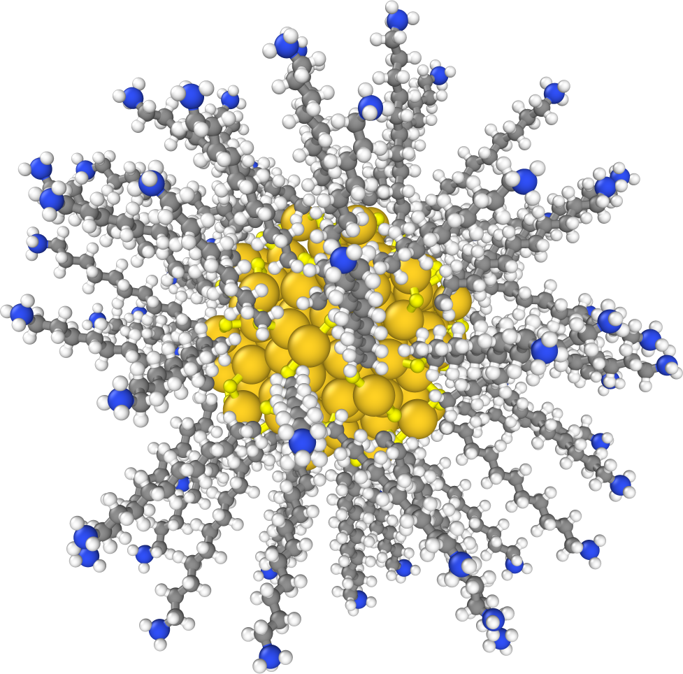
Figure 2: Ligand-protected Au nanocluster [58] composed of 2424 atoms with 6384 valence electrons used for testing parallel performance. Rendered using ovito [61].

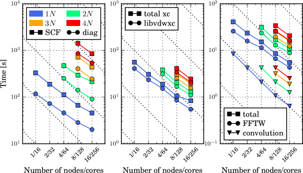
Figure 3: Scaling benchmarks for libvdwxc. Left: Time per full self-consistent field (SCF) step in DFT calculation (squares) as a function of number of compute nodes, each with 16 cores, calculated for 1 (blue), 2 (green), 3 (orange) and 4 (red) repetitions of the nanocluster test system (see Fig. 2). Also shown is the time hereof spent diagonalizing the Hamiltonian (circles), which is the most expensive part of the SCF step. Dotted lines indicate perfect parallel scaling. Middle: Timing spent for full XC calculation (libvdwxc + semilocal + distribution of data) (squares) and, hereof, time spent in libvdwxc (circles). Right: Time spent in libvdwxc (squares) and, hereof, time spent doing FFTs and convolution. The remaining operations are inexpensive.

Figure 3 shows the scaling of large calculations based on the nanoparticle system described above. Since there is no single natural choice for the main Gpaw parallelization parameters (ScaLAPACK layout, domain decomposition and band parallelization), these parameters were chosen on a best-effort basis for each system. As a result, the timings shown in the left-most figure ought be considered only representative. The libvdwxc timings do not depend on those parameters, however, so timings in the remaining figures are consistent. libvdwxc uses the standard FFTW-MPI distribution with the (automatically chosen) blocksize that most evenly divides the number of grid points. Overall the libvdwxc calculation performs in the strong scaling limit at least as well as the $\mathcal{O}(N^{3})$ diagonalization. Note that for simplicity we have benchmarked only with FFTW-MPI (not the more scalable PFFT).

Calculations normally use the larger dzp basis sets. This would make the vdW part of the calculation less expensive in comparison; the test therefore represents a worst-case comparison of vdW performance with respect to the overall DFT calculation. Real-space or planewave calculations of a system of this size would be even more expensive.

6 The library

libvdwxc is written in C and uses the standard GNU build system, autotools, for compilation. Software requirements are the FFTW3 library, an MPI library (for parallelism), and optionally the PFFT library. These can be specified at compilation time. The installation produces the main library (libvdwxc.so or libvdwxc.a) plus Fortran bindings.

A calculation comprises the following steps:

1. Call vdwxc_new to create an empty vdwxc_data data structure for a given vdW functional. The vdwxc_data structure contains the internal data associated with a calculation and is always passed as a handle to libvdwxc functions.

2. Call vdwxc_set_unit_cell to specify the number of grid points in each direction as well as the unit cell.

3. Call one of vdwxc_init_serial, vdwxc_init_mpi, or vdwxc_init_pfft to initialize the FFTW backend and allocate the necessary memory.

4. Call vdwxc_calculate any number of times, passing pointers to arrays with the input density and output potential.

5. Call vdwxc_finalize to deallocate the memory.

All calculations use double precision floating point numbers. Further convenience functions are provided, e.g., to print the state of a vdwxc_data data structure, or to check which of the optional libraries are available at runtime.

The code below illustrates the simplest possible form of a program using libvdwxc:

⬇

#include <stdio.h>

#include <vdwxc.h>

void main()

{

double rho[] = {1.0, 2.0, 3.0, 4.0}; // input: density & gradient

double sigma[] = {0.5, 1.5, 2.5, 3.5};

double dedrho[] = {0.0, 0.0, 0.0, 0.0}; // output: derivatives

double dedsigma[] = {0.0, 0.0, 0.0, 0.0};

vdwxc_data vdw = vdwxc_new(VDWXC_DF1); // vdW-DF1 functional

vdwxc_set_unit_cell(vdw, 1, 2, 2, // 1x2x2 grid; then cell vectors

1.0, 0.0, 0.0, 0.0, 2.0, 0.0, 0.0, 0.0, 2.0);

vdwxc_init_serial(vdw);

double energy = vdwxc_calculate(vdw, rho, sigma, dedrho, dedsigma);

vdwxc_finalize(&vdw);

printf("Energy %f Hartree\n", energy);

}

The greatest challenge facing a DFT code developer who wants to call libvdwxc, is to redistribute the density into the correct parallel format as described in Section 3. This is difficult to generalize since DFT codes use different parallelizations, but would typically involve a call to MPI_Alltoallv after establishing suitable buffers. Nevertheless DFT codes tend to provide tools for accomplishing this task. We implemented the redistribution in Gpaw using the existing parallel Python framework. Octopus already happened to support redistributions of the required type since it uses the same FFT libraries.

libvdwxc is free software distributed under the GNU General Public License 3 or any later version. Source code and documentation are available from the homepage [62] including the current stable release, libvdwxc 0.2.0. Development takes place openly on GitLab [63].

7 Concluding remarks

libvdwxc enables the efficient computation of the non-local correlation energies and potentials of the vdW-DF functionals on massively parallel architectures. The energies are evaluated using the vdW kernel parametrization from QE [33], while support for the Gpaw kernel format [37] and others is planned. Furthermore, extending the library to support spin polarized calculations [5] is underway.

Up to now, libvdwxc has therefore been interfaced with the Gpaw and Octopus codes, which are attractive starting points for different reasons. Gpaw features an extremely efficient linear combination of atomic orbitals implementation for DFT [59] (as demonstrated in Section 5) and time-dependent DFT [60]. Octopus, on the other hand, has been used to simulate coherent charge transfer on very large supermolecular triads with non-adiabatic dynamics [64]. Since vdW forces appear to play a role in the charge separation in organic photovoltaics [65], vdW-DF functionals in Octopus are particularly appealing. Furthermore an interface for the planewave PAW code Abinit [32] is planned.

The non-local vdW functionals can be combined with the semilocal functionals from libxc [38] to form various other functionals of the vdW-DF family. Hence vdW-DF-optPBE, vdW-DF-optB88, vdW-DF-C09, vdW-DF-BEEF, and vdW-DF-mBEEF are all available in Gpaw with libvdwxc.

Tests of vdW-DF-cx on the S22 set of molecular binding curves show that binding energies and bond lengths differ somewhat across several tested vdW implementations, as is commonly the case. The deviations are, however, rather small for the tested implementations. From tests of up to 10000 atoms, we conclude that the parallel scalability of libvdwxc should be sufficient for any kind of system accessible to ordinary Kohn–Sham DFT.

We expect this library to enhance the widespread use of the vdW-DF method. We hope that the availability of an implementation that is independent from any DFT code will lead to more reliable and reproducible calculations of the small energy differences that are characteristic of vdW interactions, and that libvdwxc can serve as a common testing ground for new developments within the framework of van der Waals functionals and related methods. Indeed the spline decomposition algorithm could be adapted to entirely different non-local functionals if they are expressible as a convolution. What happens will depend on the community since libvdwxc is open to contributions.

Acknowledgements

A. H. L. acknowledges funding from the European Union’s Horizon 2020 research and innovation program under grant agreement no. 676580 with The Novel Materials Discovery (NOMAD) Laboratory, a European Center of Excellence. M. K. is grateful for Academy of Finland Postdoctoral Researcher funding under Project No. 295602. This work has been supported by the Swedish Research council (VR), the Knut and Alice Wallenberg foundation, the Swedish Foundation for Strategic Research, and the Chalmers Area of Advance Materials Science. We acknowledge access to the supercomputer Niflheim at the Department of Physics, Technical University of Denmark. A. H. L. and Y. P. thank A. L. Pacas for stimulating discussions. The authors thank Elena (Heikkilä) Kuisma for providing the test system used for the parallel benchmarks, and Kristian Berland and Carlos de Armas for further discussions. *

Appendix A $q_{0}(\boldsymbol{\mathrm{r}})$

Dion et al. [6] introduced the quantity $q_{0}$ as a modification of the local Fermi wave vector,

$$q_{0}=\frac{\epsilon_{\mathrm{xc}}^{0}}{\epsilon_{\mathrm{x}}^{\mathrm{LDA}}}k_{F},$$ (13)

where $k_{F}=(3\pi^{2}n)^{1/3}$ is the local Fermi wavevector and $\epsilon_{\mathrm{xc}}^{0}$ is the LDA energy per particle modified by a a gradient correction describing screened exchange. For spin paired system, the full expression can be written as [66]

$$q_{0}=k_{F}-\frac{4\pi}{3}\epsilon_{\mathrm{c}}^{\mathrm{LDA}}-\frac{Z_{ab}}{36}\frac{\sigma}{k_{F}n^{2}}.$$ (14)

The LDA correlation energy per particle is evaluated using the parametrization of Perdew and Wang [28],

$$\epsilon_{\mathrm{c}}^{\mathrm{LDA}}=-2A(1+\alpha_{1}r_{s})\log\left[1+\frac{1}{2A\sum_{i=1}^{4}\beta_{i}r_{s}^{i/2}}\right].$$ (15)

The constants are $A=0.031091$, $\alpha_{1}=0.2137$, $\beta_{1}=7.5957$, $\beta_{2}=3.5876$, $\beta_{3}=1.6382$, $\beta_{4}=0.49294$, and $r_{s}$ is the Wigner–Seitz radius, $r_{s}^{3}=4\pi n/3$. vdW-DF1 uses $Z_{ab}=-0.8491$ whereas vdW-DF2 uses $Z_{ab}=-1.887$. Other functionals in the vdW-DF family generally use one of these two values, and this is the only common variation of the non-local correlation energy.

For calculations that use pseudopotentials or PAW, the density is generally relatively smooth and values of $q_{0}$ are generally smaller than 5 atomic units. Therefore the $q_{0}$ grid ends at 5 a.u., and to retain good numerical behavior towards this limit, the values of $q_{0}$ are filtered through the saturation function from Ref. [30] given by

$$h_{a}(x)=a\left[1-\exp\left(-\sum_{m=1}^{12}\frac{1}{m}\left[\frac{x}{a}\right]^{m}\right)\right].$$ (16)

This function has the property that $h_{a}(x)\approx x$ for small $x$, and $h_{a}(x)\rightarrow a$ from below for $x\rightarrow\infty$. Thus, in actual computations, $q_{0}(\boldsymbol{\mathrm{r}})=h_{a=5}(q_{0}^{\mathrm{orig}}(\boldsymbol{\mathrm{r}}))$.

References

References

- [1] P. Hohenberg and W. Kohn. Inhomogeneous electron gas. Physical Review, 136:B864–B871, Nov 1964.
- [2] W. Kohn and L. J. Sham. Self-consistent equations including exchange and correlation effects. Physical Review, 140:A1133–A1138, Nov 1965.
- [3] D C Langreth, B I Lundqvist, S D Chakarova-Käck, V R Cooper, M Dion, P Hyldgaard, A Kelkkanen, J Kleis, Lingzhu Kong, Shen Li, P G Moses, E Murray, A Puzder, H Rydberg, E Schröder, and T Thonhauser. A density functional for sparse matter. Journal of Physics: Condensed Matter, 21(8):084203, 2009.
- [4] Kristian Berland, Valentino R Cooper, Kyuho Lee, Elsebeth Schröder, T Thonhauser, Per Hyldgaard, and Bengt I Lundqvist. van der Waals forces in density functional theory: a review of the vdW-DF method. Reports on Progress in Physics, 78(6):066501, 2015.
- [5] T. Thonhauser, S. Zuluaga, C. A. Arter, K. Berland, E. Schröder, and P. Hyldgaard. Spin signature of nonlocal correlation binding in metal-organic frameworks. Physical Review Letters, 115(13):136402, 2015.
- [6] M. Dion, H. Rydberg, E. Schröder, D. C. Langreth, and B. I. Lundqvist. Van der Waals density functional for general geometries. Physical Review Letters, 92:246401, Jun 2004.
- [7] M. Dion, H. Rydberg, E. Schröder, D. C. Langreth, and B. I. Lundqvist. Erratum: Van der Waals density functional for general geometries [phys. rev. lett. 92, 246401 (2004)]. Physical Review Letters, 95:109902, Sep 2005.
- [8] Kyuho Lee, Éamonn D. Murray, Lingzhu Kong, Bengt I. Lundqvist, and David C. Langreth. Higher-accuracy van der Waals density functional. Physical Review B, 82:081101, Aug 2010.
- [9] Valentino R. Cooper. van der Waals density functional: An appropriate exchange functional. Physical Review B, 81(16):161104, 2010.
- [10] Kristian Berland and Per Hyldgaard. Exchange functional that tests the robustness of the plasmon description of the van der Waals density functional. Physical Review B, 89:035412, Jan 2014.
- [11] Jiří Klimeš, David R. Bowler, and Angelos Michaelides. Van der Waals density functionals applied to solids. Physical Review B, 83:195131, May 2011.
- [12] Ikutaro Hamada. van der Waals density functional made accurate. Physical Review B, 89(12):121103, 2014.
- [13] Jiří Klimeš, David R Bowler, and Angelos Michaelides. Chemical accuracy for the van der Waals density functional. Journal of Physics: Condensed Matter, 22(2):022201, 2010.
- [14] Jess Wellendorff, Keld T. Lundgaard, Andreas Møgelhøj, Vivien Petzold, David D. Landis, Jens K. Nørskov, Thomas Bligaard, and Karsten W. Jacobsen. Density functionals for surface science: Exchange-correlation model development with Bayesian error estimation. Physical Review B, 85:235149, Jun 2012.
- [15] Keld T. Lundgaard, Jess Wellendorff, Johannes Voss, Karsten W. Jacobsen, and Thomas Bligaard. mBEEF-vdW: Robust fitting of error estimation density functionals. Physical Review B, 93:235162, Jun 2016.
- [16] Oleg A. Vydrov and Troy Van Voorhis. Nonlocal van der Waals density functional: The simpler the better. J. Chem. Phys., 133(24):244103, 2010.
- [17] Riccardo Sabatini, Tommaso Gorni, and Stefano de Gironcoli. Nonlocal van der waals density functional made simple and efficient. Phys. Rev. B, 87:041108, Jan 2013.
- [18] Kristian Berland, Calvin Arter, Valentino R. Cooper, Kuyho Lee, Bengt I. Lundqvist, Elsebeth Schröder, Timo Thonhauser, and Per Hyldgaard. van der Waals density functionals built upon the electron-gas tradition: Facing the challenge of competing interactions. Journal of Chemical Physics, 140:18A539, 2014.
- [19] Leili Gharaee, Paul Erhart, and Per Hyldgaard. Finite-temperature properties of nonmagnetic transition metals: Comparison of the performance of constraint-based semilocal and nonlocal functionals. Physical Review B, 95:085147, Feb 2017.
- [20] Torbjörn Björkman. Testing several recent van der Waals density functionals for layered structures. J. Chem. Phys., 141:074708, 2014.
- [21] Paul Erhart, Per Hyldgaard, and Daniel O. Lindroth. Microscopic origin of thermal conductivity reduction in disordered van der Waals solids. Chemistry of Materials, 27(16):5511–5518, August 2015.
- [22] Daniel O. Lindroth and Paul Erhart. Thermal transport in van der Waals solids from first-principles calculations. Physical Review B, 94(11):115205, September 2016.
- [23] Manoharan Muruganathan, Jian Sun, Tomonori Imamura, and Hiroshi Mizuta. Electrically tunable van der Waals interaction in graphene-molecule complex. Nano Letters, 15(12):8176–8180, 2015.
- [24] Joakim Löfgren, Henrik Grönbeck, Kasper Moth-Poulsen, and Paul Erhart. Understanding the phase diagram of self-assembled monolayers of alkanethiolates on gold. The Journal of Physical Chemistry C, 120:12059, May 2016.
- [25] Mikael Juhani Kuisma, Angelica M Lundin, Kasper Moth-Poulsen, Per Hyldgaard, and Paul Erhart. A comparative ab-initio study of substituted norbornadiene-quadricyclane compounds for solar thermal storage. The Journal of Physical Chemistry C, 120:3635, January 2016.
- [26] Tonatiuh Rangel, Kristian Berland, Sahar Sharifzadeh, Florian Brown-Altvater, Kyuho Lee, Per Hyldgaard, Leeor Kronik, and Jeffrey B. Neaton. Structural and excited-state properties of oligoacene crystals from first principles. Physical Review B, 93:115206, Mar 2016.
- [27] Florian Brown-Altvater, Tonatiuh Rangel, and Jeffrey B. Neaton. Ab initio phonon dispersion in crystalline naphthalene using van der Waals density functionals. Physical Review B, 93:195206, May 2016.
- [28] John P. Perdew and Yue Wang. Accurate and simple analytic representation of the electron-gas correlation energy. Physical Review B, 45:13244–13249, Jun 1992.
- [29] Per Hyldgaard, Kristian Berland, and Elsebeth Schröder. Interpretation of van der Waals density functionals. Physical Review B, 90:075148, Aug 2014.
- [30] Guillermo Román-Pérez and José M. Soler. Efficient implementation of a van der waals density functional: Application to double-wall carbon nanotubes. Physical Review Letters, 103:096102, Aug 2009.
- [31] José M Soler, Emilio Artacho, Julian D Gale, Alberto García, Javier Junquera, Pablo Ordejón, and Daniel Sánchez-Portal. The SIESTA method for ab initio order- materials simulation. Journal of Physics: Condensed Matter, 14(11):2745, 2002.
- [32] X. Gonze, B. Amadon, P.-M. Anglade, J.-M. Beuken, F. Bottin, P. Boulanger, F. Bruneval, D. Caliste, R. Caracas, M. Côté, T. Deutsch, L. Genovese, Ph. Ghosez, M. Giantomassi, S. Goedecker, D.R. Hamann, P. Hermet, F. Jollet, G. Jomard, S. Leroux, M. Mancini, S. Mazevet, M.J.T. Oliveira, G. Onida, Y. Pouillon, T. Rangel, G.-M. Rignanese, D. Sangalli, R. Shaltaf, M. Torrent, M.J. Verstraete, G. Zerah, and J.W. Zwanziger. ABINIT: First-principles approach to material and nanosystem properties. Computer Physics Communications, 180(12):2582 – 2615, 2009.
- [33] Paolo Giannozzi, Stefano Baroni, Nicola Bonini, Matteo Calandra, Roberto Car, Carlo Cavazzoni, Davide Ceresoli, Guido L Chiarotti, Matteo Cococcioni, Ismaila Dabo, Andrea Dal Corso, Stefano de Gironcoli, Stefano Fabris, Guido Fratesi, Ralph Gebauer, Uwe Gerstmann, Christos Gougoussis, Anton Kokalj, Michele Lazzeri, Layla Martin-Samos, Nicola Marzari, Francesco Mauri, Riccardo Mazzarello, Stefano Paolini, Alfredo Pasquarello, Lorenzo Paulatto, Carlo Sbraccia, Sandro Scandolo, Gabriele Sclauzero, Ari P Seitsonen, Alexander Smogunov, Paolo Umari, and Renata M Wentzcovitch. QUANTUM ESPRESSO: a modular and open-source software project for quantum simulations of materials. Journal of Physics: Condensed Matter, 21(39):395502, 2009.
- [34] G. Kresse and J. Furthmüller. Efficiency of ab-initio total energy calculations for metals and semiconductors using a plane-wave basis set. Comput. Mater. Sci., 6(1):15–50, 1996.
- [35] J Enkovaara, C Rostgaard, J J Mortensen, J Chen, M Dułak, L Ferrighi, J Gavnholt, C Glinsvad, V Haikola, H A Hansen, H H Kristoffersen, M Kuisma, A H Larsen, L Lehtovaara, M Ljungberg, O Lopez-Acevedo, P G Moses, J Ojanen, T Olsen, V Petzold, N A Romero, J Stausholm-Møller, M Strange, G A Tritsaris, M Vanin, M Walter, B Hammer, H Häkkinen, G K H Madsen, R M Nieminen, J K Nørskov, M Puska, T T Rantala, J Schiøtz, K S Thygesen, and K W Jacobsen. Electronic structure calculations with GPAW: A real-space implementation of the projector augmented-wave method. Journal of Physics: Condensed Matter, 22(25):253202, 2010.
- [36] Xavier Andrade, David Strubbe, Umberto De Giovannini, Ask Hjorth Larsen, Micael J. T. Oliveira, Joseba Alberdi-Rodriguez, Alejandro Varas, Iris Theophilou, Nicole Helbig, Matthieu J. Verstraete, Lorenzo Stella, Fernando Nogueira, Alan Aspuru-Guzik, Alberto Castro, Miguel A. L. Marques, and Angel Rubio. Real-space grids and the Octopus code as tools for the development of new simulation approaches for electronic systems. Phys. Chem. Chem. Phys., pages 31371–31396, 2015.
- [37] Jess Wellendorff, André Kelkkanen, Jens Jørgen Mortensen, Bengt I. Lundqvist, and Thomas Bligaard. RPBE-vdW description of benzene adsorption on Au(111). Topics in Catalysis, 53(5):378–383, 2010.
- [38] Miguel A.L. Marques, Micael J.T. Oliveira, and Tobias Burnus. Libxc: A library of exchange and correlation functionals for density functional theory. Computer Physics Communications, 183(10):2272 – 2281, 2012.
- [39] Matteo Frigo and Steven G. Johnson. The design and implementation of FFTW3. Proceedings of the IEEE, 93(2):216–231, 2005. Special issue on “Program Generation, Optimization, and Platform Adaptation”.
- [40] Michael Pippig. PFFT - An extension of FFTW to massively parallel architectures. SIAM J. Sci. Comput., 35:C213 – C236, 2013.
- [41] Pier Luigi Silvestrelli. Van der Waals interactions in DFT made easy by Wannier functions. Physical Review Letters, 100:053002, Feb 2008.
- [42] Pier Luigi Silvestrelli. Van der Waals interactions in density functional theory using wannier functions. Journal of Physical Chemistry A, 113:5224, 2009.
- [43] Alexandre Tkatchenko and Matthias Scheffler. Accurate molecular van der Waals interactions from ground-state electron density and free-atom reference data. Physical Review Letters, 102:073005, Feb 2009.
- [44] Stefan Grimme. Semiempirical GGA-type density functional constructed with a long-range dispersion correction. Journal of Computational Chemistry, 27(15):1787–1799, 2006.
- [45] Stefan Grimme, Stephan Ehrlich, and Lars Goerigk. Effect of the damping function in dispersion corrected density functional theory. Journal of Computational Chemistry, 32(7):1456–1465, 2011.
- [46] Axel D. Becke and Erin R. Johnson. Exchange-hole dipole moment and the dispersion interaction. The Journal of Chemical Physics, 122(15):154104, 2005.
- [47] Kristian Berland, Øyvind Borck, and Per Hyldgaard. Van der waals density functional calculations of binding in molecular crystals. Computer Physics Communications, 182(9):1800 – 1804, 2011. Computer Physics Communications Special Edition for Conference on Computational Physics Trondheim, Norway, June 23-26, 2010.
- [48] Fabiano Corsetti, Emilio Artacho, José M. Soler, S. S. Alexandre, and M.-V. Fernández-Serra. Room temperature compressibility and diffusivity of liquid water from first principles. The Journal of Chemical Physics, 139(19):194502, 2013.
- [49] Pablo García-Risueño, Joseba Alberdi-Rodriguez, Micael J. T. Oliveira, Xavier Andrade, Michael Pippig, Javier Muguerza, Agustin Arruabarrena, and Angel Rubio. A survey of the parallel performance and accuracy of Poisson solvers for electronic structure calculations. Journal of Computational Chemistry, 35(6):427–444, 2014.
- [50] J. J. Mortensen, L. B. Hansen, and K. W. Jacobsen. Real-space grid implementation of the projector augmented wave method. Physical Review B, 71:035109, Jan 2005.
- [51] G. Kresse and J. Furthmüller. Efficient iterative schemes for ab initio total-energy calculations using a plane-wave basis set. Physical Review B, 54:11169, 1996.
- [52] Petr Jurecka, Jiri Sponer, Jiri Cerny, and Pavel Hobza. Benchmark database of accurate (MP2 and CCSD(T) complete basis set limit) interaction energies of small model complexes, DNA base pairs, and amino acid pairs. Physical Chemistry Chemical Physics, 8:1985–1993, 2006.
- [53] D. R. Hamann. Optimized norm-conserving Vanderbilt pseudopotentials. Physical Review B, 88:085117, Aug 2013.
- [54] P. E. Blöchl. Projector augmented-wave method. Physical Review B, 50:17953–17979, Dec 1994.
- [55] P. Lazić, N. Atodiresei, V. Caciuc, R. Brako, B. Gumhalter, and S. Blügel. Rationale for switching to nonlocal functionals in density functional theory. Journal of Physics: Condensed Matter, 24:424215, 2012.
- [56] Kristian Berland and Per Hyldgaard. Analysis of van der Waals density functional components: Binding and corrugation of benzene and C60 on boron nitride and graphene. Physical Review B, 87:205421, 2013.
- [57] Ask Hjorth Larsen, Jens Mortensen, Jakob Blomqvist, Ivano Castelli, Rune Christensen, Marcin Dulak, Jesper Friis, Michael Groves, Bjork Hammer, Cory Hargus, Eric Hermes, Paul Jennings, Peter Jensen, James Kermode, John Kitchin, Esben Kolsbjerg, Joseph Kubal, Kristen Kaasbjerg, Steen Lysgaard, Jon Maronsson, Tristan Maxson, Thomas Olsen, Lars Pastewka, Andrew Peterson, Carsten Rostgaard, Jakob Schiøtz, Ole Schütt, Mikkel Strange, Kristian Thygesen, Tejs Vegge, Lasse Vilhelmsen, Michael Walter, Zhenhua Zeng, and Karsten Wedel Jacobsen. The Atomic Simulation Environment — A Python library for working with atoms. Journal of Physics: Condensed Matter, 2017.
- [58] Elena Heikkilä, Andrey A. Gurtovenko, Hector Martinez-Seara, Hannu Häkkinen, Ilpo Vattulainen, and Jaakko Akola. Atomistic simulations of functional Au144(SR)60 gold nanoparticles in aqueous environment. The Journal of Physical Chemistry C, 116(17):9805–9815, 2012.
- [59] A. H. Larsen, M. Vanin, J. J. Mortensen, K. S. Thygesen, and K. W. Jacobsen. Localized atomic basis set in the projector augmented wave method. Physical Review B, 80:195112, Nov 2009.
- [60] M. Kuisma, A. Sakko, T. P. Rossi, A. H. Larsen, J. Enkovaara, L. Lehtovaara, and T. T. Rantala. Localized surface plasmon resonance in silver nanoparticles: Atomistic first-principles time-dependent density-functional theory calculations. Physical Review B, 91:115431, Mar 2015.
- [61] Alexander Stukowski. Visualization and analysis of atomistic simulation data with OVITO–the Open Visualization Tool. Modelling and Simulation in Materials Science and Engineering, 18(1):015012, 2010.
- [62] libvdwxc homepage. https://libvdwxc.gitlab.io/libvdwxc.
- [63] libvdwxc on gitlab. https://gitlab.com/libvdwxc/libvdwxc.
- [64] Carlo Andrea Rozzi, Sarah Maria Falke, Nicola Spallanzani, Angel Rubio, Elisa Molinari, Daniele Brida, Margherita Maiuri, Giulio Cerullo, Heiko Schramm, Jens Christoffers, and Christoph Lienau. Quantum coherence controls the charge separation in a prototypical artificial light-harvesting system. Nature Communications, 4:1602, Mar 2013.
- [65] Topi Karilainen, Oana Cramariuc, Mikael Kuisma, Kirsi Tappura, and Terttu I. Hukka. van der Waals interactions are critical in Car–Parrinello molecular dynamics simulations of porphyrin–fullerene dyads. Journal of Computational Chemistry, 36(9):612–621, 2015.
- [66] T. Thonhauser, Valentino R. Cooper, Shen Li, Aaron Puzder, Per Hyldgaard, and David C. Langreth. Van der waals density functional: Self-consistent potential and the nature of the van der waals bond. Phys. Rev. B, 76:125112, Sep 2007.