Exclusive $\eta$ electroproduction at $W>2$ GeV with CLAS
and transversity generalized parton distributions

Abstract

The cross section of the exclusive $\eta$ electroproduction reaction $ep\to e^{\prime}p^{\prime}\eta$ was measured at Jefferson Lab with a 5.75-GeV electron beam and the CLAS detector. Differential cross sections $d^{4}\sigma/dtdQ^{2}dx_{B}d\phi_{\eta}$ and structure functions $\sigma_{U}=\sigma_{T}+\epsilon\sigma_{L},\sigma_{TT}$ and $\sigma_{LT}$, as functions of $t$ were obtained over a wide range of $Q^{2}$ and $x_{B}$. The $\eta$ structure functions are compared with those previously measured for $\pi^{0}$ at the same kinematics. At low $t$, both $\pi^{0}$ and $\eta$ are described reasonably well by generalized parton distributions (GPDs) in which chiral-odd transversity GPDs are dominant. The $\pi^{0}$ and $\eta$ data, when taken together, can facilitate the flavor decomposition of the transversity GPDs.

I Introduction

Understanding nucleon structure in terms of the fundamental degrees of freedom of Quantum Chromodynamics (QCD) is one of the main goals in the theory of strong interactions. Exclusive reactions may provide information about the quark and gluon distributions encoded in Generalized Parton Distributions (GPDs), which are accessed via application of the handbag mechanism Ji (1997a); *Ji:1996nm; Radyushkin (1996); *Radyushkin:1997ki . Deeply virtual meson electroproduction (DVMP), specifically for pseudoscalar meson production, e.g., $\eta$ and $\pi^{0}$, is shown schematically in Fig. 1.

Figure 1: The handbag diagram for deeply virtual $\eta$ and $\pi^{0}$ production. The helicities of the initial and final nucleons are denoted by $\nu$ and $\nu^{\prime}$, of the incident photon and produced meson by $\mu$ and $\mu^{\prime}$ and of the active initial and final quark by $\lambda$ and $\lambda^{\prime}$. The arrows in the figure represent schematically the corresponding positive and negative helicities, respectively. For final-state pseudoscalar mesons $\mu^{\prime}=0$.

For each quark flavor there are eight leading-twist GPDs. Four correspond to parton helicity-conserving (chiral-even) processes, denoted by $H^{i}$, $\tilde{H}^{i}$, $E^{i}$ and $\tilde{E}^{i}$, and four correspond to parton helicity-flip (chiral-odd) processes Hoodbhoy and Ji (1998); Diehl (2003), $H^{i}_{T}$, $\tilde{H}^{i}_{T}$, $E^{i}_{T}$ and $\tilde{E}^{i}_{T}$, where $i$ denotes quark flavor. The GPDs depend on three kinematic variables: $x$, $\xi$ and $t$, where $x$ is the average longitudinal momentum fraction of the struck parton before and after the hard interaction and $\xi$ (skewness) is half of the longitudinal momentum fraction transferred to the struck parton. Denoting $q$ as the four-momentum transfer and $Q^{2}=-q^{2}$, the skewness for light mesons of mass $m$, in which $m^{2}/Q^{2}\ll 1$, can be expressed in terms of the Bjorken variable $x_{B}$ as $\xi\simeq x_{B}/(2-x_{B})$. Here $x_{B}=Q^{2}/(2p\cdot q)$ and $t=(p-p^{\prime})^{2}$, where $p$ and $p^{\prime}$ are the initial and final four-momenta of the nucleon. Since the $\pi^{0}$ and $\eta$ have different combinations of quark flavors, it may be possible to approximately make a flavor decomposition of the GPDs for up and down quarks.

When the leading order chiral even theoretical calculations for longitudinal virtual photons were compared with the Jefferson Lab $\pi^{0}$ data Bedlinskiy et al. (2012, 2014) they were found to underestimate the measured cross sections by more than an order of magnitude in their accessible kinematic regions. The failure to describe the experimental results with quark helicity-conserving operators stimulated a consideration of the role of the chiral-odd quark helicity-flip processes. Pseudoscalar meson electroproduction was identified as especially sensitive to the quark helicity-flip subprocesses. During the past few years, two parallel theoretical approaches - Goloskokov and Kroll (2009, 2011) (GK) and Ahmad et al. (2009)  (GL) - have been developed utilizing the chiral-odd GPDs in the calculation of pseudoscalar meson electroproduction. The GL and GK approaches, although employing different models of GPDs, lead to transverse photon amplitudes that are much larger than the longitudinal amplitudes. This has been recently confirmed experimentally for $t$ near $t_{min}$ Defurne et al. (2016).

II Experimental setup

The measurements reported here were carried out with the CEBAF Large Acceptance Spectrometer (CLAS) Mecking et al. (2003) located in Hall B at Jefferson Lab. The data were obtained in 2005 in parallel with our previously reported deeply virtual Compton scattering (DVCS) and $\pi^{0}$ electroproduction experiments Bedlinskiy et al. (2012, 2014); Girod et al. (2008); Jo et al. (2015); Masi et al. (2008), sharing the same physical setup. The integrated luminosity corresponding to the data presented here was $20$ fb^-1.

The spectrometer consisted of a toroidal-like magnetic field produced by six current coils symmetrically arrayed around the beam axis that divided the detector into six sectors. The scheme of the CLAS detector array, as coded in the GEANT3-based CLAS simulation code GSIM Wolin (1996), is shown in Fig. 2.

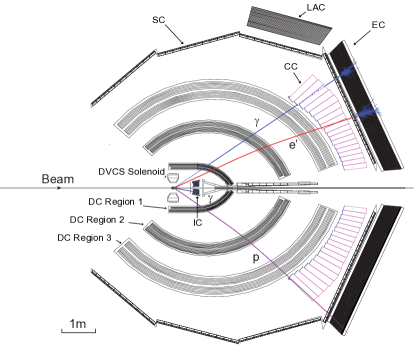
Figure 2: (Color online) Schematic view of the CLAS detector in the plane of the beamline constructed by the Monte Carlo simulation program GSIM. The notation is as follows: inner calorimeter (IC) , electromagnetic calorimeter (EC), large angle electromagnetic calorimeter (LAC), Cherenkov counter (CC), scintillation hodoscope (SC), Drift Chambers (DC). The LAC was not used in this analysis. The tracks correspond, from top to bottom, to a photon (blue online), an electron (red online) curving toward the beam line, and a proton (purple online) curving away from the beam line.

The data were taken using a 5.75 GeV incident electron beam impinging a 2.5 cm long liquid hydrogen target. The electron beam was about 80% polarized. The sign of the beam polarization was changed during measurements at a frequency of 30 Hz. We did not use beam polarization information in this analysis. Effectively, for this experiment the beam was unpolarized. The target was placed 66 cm upstream of the nominal center of CLAS inside a solenoid magnet to shield the detectors from Møller electrons.

Each sector was equipped with three regions of drift chambers (DC) Mestayer et al. (2000) to determine the trajectory of charged particles, gas threshold Cherenkov counters (CC) Adams et al. (2001) for electron identification, a scintillation hodoscope Smith et al. (1999) for time-of-flight (TOF) measurements of charged particles, and an electromagnetic calorimeter (EC) Amarian et al. (2001) that was used for electron identification as well as detection of neutral particles. To detect photons at small polar angles (from 4.5^∘ up to 15^∘) an inner calorimeter (IC) was added to the standard CLAS configuration, 55 cm downstream from the target. The IC consisted of 424 PbWO₄ tapered crystals whose orientations were projected approximately toward the target. Figure 3 zooms in on the target area of Fig. 2 to better illustrate the deployment of the IC and solenoid relative to the target.

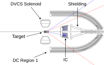
Figure 3: (Color online) A blowup of Fig. 2 showing the CLAS target region in detail. IC is the inner calorimeter and DC Region 1 represents the drift chambers closest to the target.

The toroidal magnet was operated at a current corresponding to an integral magnetic field of about 1.36 T-m in the forward direction. The magnet polarity was set such that negatively charged particles were bent inward towards the electron beam line. The scattered electrons were detected in the CC and EC, which extended from 21^∘ to 45^∘. The lower angle limit was defined by the IC calorimeter, which was located just after the target.

A Faraday cup was used for the integrated charge measurement with 1% accuracy. It was composed of 4000 kg of lead, which corresponds to 75 radiation lengths, and was located 29 m downstream of the target.

In the experiment, all four final state particles of the reaction $ep\to e^{\prime}p^{\prime}\eta,\ \eta\to\gamma\gamma$ were detected. The kinematic coverage for this reaction is shown in Fig. 4, and for the individual kinematic variables in Fig. 5. For the purpose of physics analysis an additional cut on $W>2$ GeV was applied as well, where $W$ is the $\gamma^{*}p$ center-of-mass energy.

The basic configuration of the trigger included the coincidence between signals from the CC and the EC in the same sector, with a threshold $\sim 500$ MeV. This was the general trigger for all experiments in this run period. This threshold is far from the kinematic limit of this experiment - $E^{\prime}>$ 0.8 GeV (see Fig.4). The accepted region (yellow online) for this experiment is determined by the following cuts: $W>2$ GeV, $E^{\prime}>$ 0.8 GeV, $21^{\circ}<\theta<45^{\circ}$. Out of a total of about $7\times 10^{9}$ recorded events, about $20\times 10^{3}$, in 1200 kinematic bins in $Q^{2},t,x_{B}$ and $\phi_{\eta}$, for the reaction $ep\to e^{\prime}p^{\prime}\eta$, were finally retained. The variable $\phi_{\eta}$ is the azimuthal angle of the emitted $\eta$ relative to the electron scattering plane.

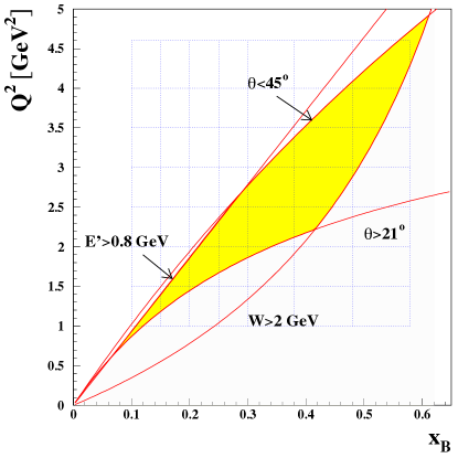
Figure 4: (Color online) The kinematic coverage and binning as a function of $Q^{2}$ and $x_{B}$. The accepted region (yellow online) is determined by the following cuts: $W>2$ GeV, $E^{\prime}>$ 0.8 GeV, $21^{\circ}<\theta<45^{\circ}$. $W$ is the $\gamma^{*}p$ center-of-mass energy, $E^{\prime}$ is the scattered electron energy and $\theta$ is the electron’s polar angle in the lab frame. The accepted yellow region within each grid boundary represents the kinematic regions for which the cross sections are calculated and presented.

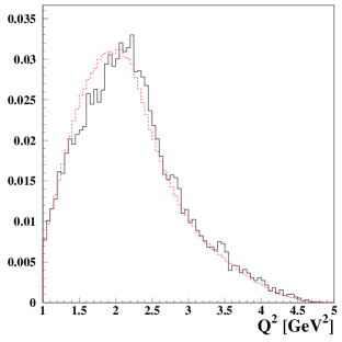
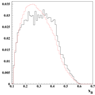
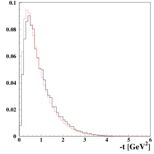
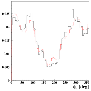
Figure 5: (Color online) Yield distributions for kinematic variables $Q^{2}$, $x_{B}$, $-t$ and $\phi_{\eta}$ in arbitrary units. The data are in black (solid) and the results of Monte Carlo simulations (see Sec. VI) are in red (dotted). The areas under the curves are normalized to each other. The curves for both the data and Monte Carlo simulations are the final distributions obtained after tracking and include acceptances and efficiencies.

III Particle Identification

III.1 Electron identification

An electron was identified by requiring the track of a negatively charged particle in the DCs to be matched in space with hits in the CC, the SC and the EC. This electron selection effectively suppresses $\pi^{-}$ contamination up to momenta $\sim$2.5 GeV, which is approximately the threshold for Cherenkov radiation of the $\pi^{-}$ in the CC. Additional requirements were used in the offline analysis to refine electron identification and to suppress the remaining pions.

Energy deposition cuts on the electron signal in the EC also play an important role in suppressing the pion background. An electron propagating through the calorimeter produces an electromagnetic shower and deposits a large fraction of its energy in the calorimeter proportional to its momentum, while pions typically lose a smaller fraction of their energy, primarily by ionization.

The distribution of the number of the photoelectrons in the CC after all selection criteria were applied is shown in Fig. 6. The residual small shoulder around $N_{phe}=1$ represents the pion contamination, which is seen to be negligibly small after applying all selection criteria.

Figure 6: The number of CC photoelectrons for events that pass all cuts.

The charged particle tracks were reconstructed by the drift chambers. The vertex location was calculated from the intersection of the track with the beam line. A cut was applied on the $z$-component of the electron vertex position to eliminate events originating outside the target. The vertex distribution and cuts for one of the sectors are shown in Fig. 7. The left plot shows the $z$-coordinate distribution before the exclusivity cuts, which are described below in Section IV.2, and the right plot is the distribution after the exclusivity cuts. The peak at $z=-62.5$ cm exhibits the interaction of the beam with an insulating foil, which is completely removed after the application of the exclusivity cuts, demonstrating that these cuts very effectively exclude the interactions involving nuclei of the surrounding nontarget material.

(a) Before any exclusivity cuts.

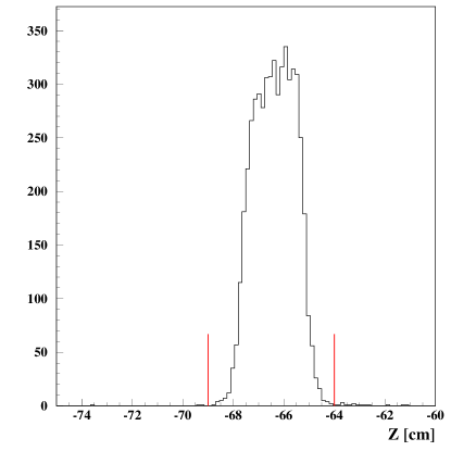
(b) After $\eta$ exclusivity cuts.

Figure 7: The $z$-coordinate of the electron vertex. The vertical lines are the positions of the applied cuts. Note in (a) the small peak to the right of the target that is due to a foil placed at $z=-62.5$ cm downstream of the target window. In panel (b) the peak due to the foil disappears after the selection of the exclusive reaction.

III.2 Proton identification

The proton was identified as a positively charged particle with the correct time-of-flight. The quantity of interest ($\delta t=t_{SC}-t_{exp}$) is the difference in the time between the measured flight time from the event vertex to the SC system ($t_{SC}$) and that expected for the proton ($t_{exp}$). The quantity $t_{exp}$ was computed from the velocity of the particle and the track length. The velocity was determined from the momentum by assuming the mass of the particle equals that of a proton. A cut at the level of $\pm 5\sigma_{t}$ was applied around $\delta t=0$, where $\sigma_{t}$ is the time-of-flight resolution, which is momentum dependent. This wide cut was possible because the exclusivity cuts (see Section IV B below) very effectively suppressed the remaining pion contamination.

III.3 Photon identification

Photons were detected in both calorimeters, the EC and IC. In the EC, photons were identified as neutral particles with $\beta>0.8$ and $E>0.35$ GeV. Fiducial cuts were applied to avoid the EC edges. When a photon hits the boundary of the calorimeter, the energy cannot be fully reconstructed due to the leakage of the shower out of the detector. Additional fiducial cuts on the EC were applied to account for the shadow of the IC (see Fig. 2). The calibration of the EC was done using cosmic muons and the photons from neutral pion decay ($\pi^{0}\to\gamma\gamma$).

In the IC, each detected cluster was considered a photon. The assumption was made that this photon originated from the electron vertex. Additional geometric cuts were applied to remove low-energy clusters around the beam axis and photons near the edges of the IC, where the energies of the photons were incorrectly reconstructed due to the electromagnetic shower leakage. The photons from $\eta\to\gamma\gamma$ decays were detected in the IC in an angular range between $5^{\circ}$ and $17^{\circ}$ and in the EC for angles greater than $21^{\circ}$. The reconstructed invariant mass of two-photon events was then subjected to various cuts to isolate exclusive $\eta$ events, with a residual background, as discussed in Section IV B below.

III.4 Kinematic corrections

Ionization energy-loss corrections were applied to protons and electrons in both data and Monte Carlo events. These corrections were estimated using the GSIM Monte Carlo program. Due to imperfect knowledge of the properties of the CLAS detector, such as the magnetic field distribution and the precise placement of the components or detector materials, small empirical sector-dependent corrections had to be made on the momenta and angles of the detected electrons and protons. The corrections were determined by systematically studying the kinematics of the particles emitted from well understood kinematically-complete processes, e.g., elastic electron scattering. These corrections were on the order of 1%.

IV Event selection

IV.1 Fiducial cuts

Certain areas of the detector acceptance were not efficient due to gaps in the DC, problematic SC counters, and inefficient zones of the CC and the EC. These areas were removed from the analysis as well as from the simulation by means of geometrical cuts, which were momentum, polar angle and azimuthal angle dependent.

In addition, we excluded events, when a photon from the $\eta$-decay or Bremsstrahlungs photon was detected in the same sector as the electron. This avoids additional photons which are close in space to the scattered lepton leaving a signal in the EC close to where the supposed lepton hits the EC. This was done for both the experimental data as well as the Monte Carlo data used for correcting experimental yields.

IV.2 Exclusivity cuts

To select the exclusive reaction $ep\rightarrow e^{\prime}p^{\prime}\eta$, each event was required to contain an electron, one proton and at least two photons in the final state. Then, so called exclusivity cuts were applied to all combinations of an electron, a proton and two photons to ensure energy and momentum conservation, thus eliminating events in which there were any additional undetected particles.

Four cuts were used for the exclusive event selection

• $\theta_{X}<2^{o}$, where $\theta_{X}$ is the angle between the reconstructed $\eta$ momentum vector and the missing momentum vector for the reaction $ep\to e^{\prime}p^{\prime}X$.

• the missing mass squared $M_{x}^{2}(e^{\prime}p^{\prime})$ of the $e^{\prime}p^{\prime}$ system ($ep\to e^{\prime}p^{\prime}X$), with $|M_{x}^{2}(e^{\prime}p^{\prime})-M^{2}_{\eta}|<3\sigma$;

• the missing mass $M_{x}(e^{\prime}\gamma\gamma)$ of the $e^{\prime}\gamma\gamma$ system ($ep\to e^{\prime}\gamma\gamma X$), with $|M_{x}(e^{\prime}\gamma\gamma)-M_{p}|<3\sigma$;

• the missing energy $E_{x}(e^{\prime}p^{\prime}\eta)$ ($ep\to e^{\prime}p^{\prime}\gamma\gamma X$), with $|E_{x}(e^{\prime}p^{\prime}\eta)-0|<3\sigma$;

Here $\sigma$ is the observed experimental resolution obtained as the standard deviation from the mean value of the distributions of each quantity. Three sets of resolutions were determined independently for each of the three photon-detection topologies (IC-IC, IC-EC, EC-EC). The invariant mass $M_{\gamma\gamma}$ for the two detected photons, where both photons were detected in the IC, after these cuts is shown in Fig. 8. The two peaks correspond to $\pi^{0}$ and $\eta$ production, with the $\pi^{0}$ production exhibiting a significantly larger cross section than $\eta$ production. The distributions were generally broader than in the Monte Carlo simulations so that the cuts for the data were typically broader than those used for the Monte Carlo simulations. Similar results were obtained for the topology in which one photon was detected in the IC and one in the EC, as well as the case where both photons were detected in the EC.

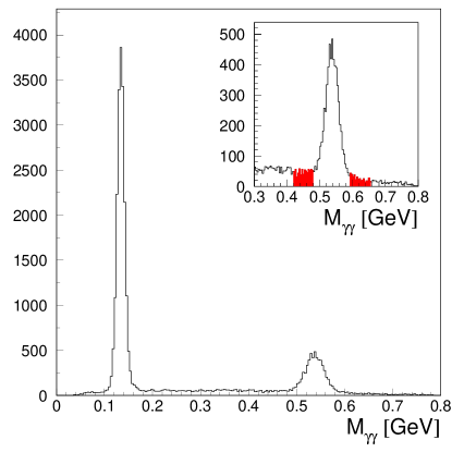
Figure 8: (Color online) The two-photon invariant mass distribution, $M_{\gamma\gamma}$, after all exclusivity cuts have been applied, for the case where the two photons are detected by the IC. The large peak at lower $M_{\gamma\gamma}$ is due to $\pi^{0}$ electroproduction and the smaller peak at higher $M_{\gamma\gamma}$ is due to $\eta$ electroproduction. The inset magnifies the region around the $\eta$ peak. The filled regions above and below the peak (red online) are the sidebands that are used for background subtraction, as discussed in the text.

IV.3 Background subtraction

The $M_{\gamma\gamma}$ distribution contains background under the $\eta$ peak even after the application of all exclusivity cuts shown in the insert of Fig. 8. The background under the $\eta$ invariant mass peak was subtracted for each kinematic bin. It was found that most of the background comes from the production of $\pi^{0}$ meson, together with the detection of only one decay photon with an accidental photon signal in the electromagnetic calorimeter. Thus, the background was subtracted using the following procedure. All $\pi^{0}$ events which were in coincidence with accidental photons were identified. Then, the distributions of the invariant masses of one of the $\pi^{0}$ decay photons with the accidentals were obtained, and normalized with respect to the side bands around the $\eta$ mass. The sidebands were determined as $(-6\sigma,-3\sigma)\cup(3\sigma,6\sigma)$ in the $M_{\gamma\gamma}$ distributions, as shown in Fig. 8.

The resulting events in the region between side bands were then subtracted as the background contamination. The mean ratio of background to peak over all kinematic bins and all combinations of IC and EC is about 25%.

IV.4 Kinematic binning

The kinematics of the reaction are defined by four variables: $Q^{2}$, $x_{B}$, $t$ and $\phi_{\eta}$. In order to obtain differential cross sections the data were divided into four-dimensional rectangular bins in these variables. There are seven bins in $x_{B}$, seven bins in $Q^{2}$ as shown in Tables 3–3 and in Fig. 4. For each $Q^{2}$-$x_{B}$ bin there are nominally eight bins in $t$ (Table  3), but the actual number is determined by the kinematic acceptance in $t$ for each $Q^{2}$-$x_{B}$ bin, as well as the available statistics. Differential cross section distributions were obtained for 20 bins in $\phi_{\eta}$ for each kinematic bin in $Q^{2}$, $x_{B}$ and $t$.

Table 1: $Q^{2}$ bins

Bin Number	Lower Limit	Upper limit
	(GeV2)	(GeV2)
1	1.0	1.5
2	1.5	2.0
3	2.0	2.5
4	2.5	3.0
5	3.0	3.5
6	3.5	4.0
7	4.0	4.6

Table 2: $x_{B}$ bins

Bin Number	Lower Limit	Upper limit
1	0.10	0.15
2	0.15	0.20
3	0.20	0.25
4	0.25	0.30
5	0.30	0.38
6	0.38	0.48
7	0.48	0.58

Table 3: $|t|$ bins

Bin Number	Lower Limit	Upper limit
	(GeV2)	(GeV2)
1	0.09	0.15
2	0.15	0.20
3	0.20	0.30
4	0.30	0.40
5	0.40	0.60
6	0.60	1.00
7	1.00	1.50
8	1.50	2.00

V Cross sections for $\gamma^{*}p\to\eta p^{\prime}$

The fourfold differential cross section as a function of the four variables $(Q^{2},x_{B},t,\phi_{\eta})$ was obtained from the expression

$$\begin{split}\frac{d^{4}\sigma_{ep\rightarrow e^{\prime}p^{\prime}\eta}}{dQ^{2}dx_{B}dtd\phi_{\eta}}=\frac{N(Q^{2},x_{B},t,\phi_{\eta})}{\Delta Q^{2}\Delta x_{B}\Delta t\Delta\phi_{\eta}}\times\\ \frac{1}{\mathcal{L}_{int}\epsilon_{ACC}\delta_{RC}\delta_{Norm}Br(\eta\to\gamma\gamma)}.\end{split}$$ (1)

The definitions of the quantities in Eq. 1 are:

• $N(Q^{2},x_{B},t,\phi_{\eta})$ is the number of $ep\rightarrow e^{\prime}p^{\prime}\eta$ events in a given ($Q^{2},x_{B},t,\phi_{\eta}$) bin;

• $\Delta Q^{2}\Delta x_{B}\Delta t\Delta\phi_{\eta}$ is the corresponding 4-dimensional bin volume. The accepted kinematic bin volumes in $Q^{2},x_{B},t,{\text{ and }}\phi_{\eta}$ are typically smaller than the product $\Delta Q^{2}\cdot\Delta x_{B}\cdot\Delta t\cdot\Delta\phi_{\eta}$ of the 4-dimensional grid because of cuts in $\theta_{e}$, $W$ and $E^{\prime}$ (e.g. see Fig. 4 ). The reported $Q^{2}$, $x_{B}$ and $t$ value for each bin is the mean value of the accepted volume assuming a constant density of events.

• $\mathcal{L}_{int}$ is the integrated luminosity (which takes into account the correction for the data-acquisition dead time);

• $\epsilon_{ACC}$ is the acceptance calculated for each bin $(Q^{2},x_{B},t,\phi_{\eta})$ (see Sec. VI) ;

• $\delta_{RC}$ is the correction factor due to the radiative effects calculated for each $(Q^{2},x_{B},t,\phi_{\eta})$ bin (see Sec. VII) ;

• $\delta_{Norm}$ is the overall absolute normalization factor calculated from the elastic cross section measured in the same experiment (see Sec. VIII);

• $Br(\eta\to\gamma\gamma)=\frac{\Gamma(\eta\to\gamma\gamma)}{\Gamma_{total}}=0.394$  Olive et al. (2014) is the branching ratio for the $\eta\to\gamma\gamma$ decay mode.

The reduced or “virtual photon” cross sections were extracted from the fourfold cross section (Eq. 1) through:

$$\frac{d^{2}\sigma_{\gamma^{*}p\rightarrow p^{\prime}\eta}}{dtd\phi_{\eta}}=\frac{1}{\Gamma_{V}(Q^{2},x_{B},E)}\frac{d^{4}\sigma_{ep\rightarrow e^{\prime}p^{\prime}\eta}}{dQ^{2}dx_{B}dtd\phi_{\eta}}.$$ (2)

The Hand convention Hand (1963) was adopted for the definition of the virtual photon flux $\Gamma_{V}$:

$$\Gamma_{V}(Q^{2},x_{B},E)=\frac{\alpha}{8\pi}\frac{Q^{2}}{m_{p}^{2}E^{2}}\frac{1-x_{B}}{x_{B}^{3}}\frac{1}{1-\epsilon},$$ (3)

where $\alpha$ is the standard electromagnetic coupling constant. The variable $\epsilon$ represents the ratio of fluxes of longitudinally and transversely polarized virtual photons and is given by

$$\epsilon=\frac{1-y-\frac{Q^{2}}{4E^{2}}}{1-y+\frac{y^{2}}{2}+\frac{Q^{2}}{4E^{2}}},$$ (4)

with $y=p\cdot q/q\cdot k=\nu/E$.

A table of the reduced cross sections can be obtained online in Ref. Bedlinskiy et al. (2016). An example of the differential cross section as a function of $\phi_{\eta}$ in a single kinematic interval in $Q^{2},t$ and $x_{B}$ is shown in Fig. 9.

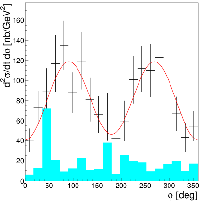
Figure 9: (Color online) The differential cross section $d^{2}\sigma/dtd\phi_{\eta}$ for the reaction $\gamma^{*}p\to p^{\prime}\eta$ for the kinematic interval at $Q^{2}=1.75$ GeV², $x_{B}=0.23$ and $t=-0.8$ GeV². The error bars indicate statistical uncertainties. Systematic uncertainties are indicated by the cyan bars. The red curve is a fit in terms of the structure functions in Eq. 7.

VI Monte Carlo simulation

The acceptance for each ($Q^{2}$, $x_{B}$, $t$, $\phi_{\eta}$) bin of the CLAS detector with the present setup for the reaction $ep\rightarrow e^{\prime}p^{\prime}\gamma\gamma$ was calculated using the Monte Carlo program GSIM. The event generator used an empirical parametrization of the cross section as a function of $Q^{2}$, $x_{B}$ and $t$. The parameters were tuned using the MINUIT program to best match the simulated $\eta$ cross section with the measured electroproduction cross section. Two iterations were found to be sufficient to describe the experimental cross section and distributions. The comparisons of the experimental and Monte Carlo simulated distributions are shown in Fig. 5 for the variables $Q^{2}$, $x_{B}$, $-t$ and $\phi_{\eta}$.

Additional smearing factors for tracking and timing resolutions were included in the simulations to provide more realistic resolutions for charged particles. The Monte Carlo events were analyzed by the same code that was used to analyze the experimental data, and with the additional smearing and somewhat different exclusivity cuts, to account for the leftover discrepancies in calorimeter resolutions. Ultimately the number of reconstructed Monte Carlo events was an order of magnitude higher than the number of reconstructed experimental events. Thus, the statistical uncertainty introduced by the acceptance calculation was typically much smaller than the statistical uncertainty of the data.

The efficiency of the event reconstruction depends on the level of noise in the detector, the greater the noise the lower the efficiency. It was found that the efficiency for reconstructing particles decreased linearly with increasing beam current. To take this into account the background hits from random 3-Hz-trigger events were mixed with the Monte Carlo events for all detectors - DC, EC, IC, SC and CC. The acceptance for a given bin was calculated as a ratio of the number of reconstructed events to the number of generated events as

$$\epsilon_{ACC}(Q^{2},x_{B},t,\phi_{\eta})=\frac{N^{rec}(Q^{2},x_{B},t,\phi_{\eta})}{N^{gen}(Q^{2},x_{B},t,\phi_{\eta})}.$$ (5)

Only areas of the 4-dimensional space with an acceptance equal to or greater than 0.5% were used. This cut was applied to avoid the regions where the calculation of the acceptance was not reliable.

VII Radiative Corrections

The QED processes include radiation of photons that are not detected by the experimental set up, as well as vacuum polarization and lepton-photon vertex corrections (see Fig. 10).

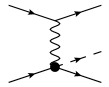
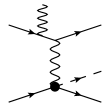
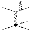
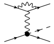
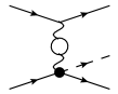
Figure 10: Feynman diagrams contributing to the $\eta$ electroproduction cross section. Left to right: Born process, Bremsstrahlung (by the initial and the final electron), vertex correction, and vacuum polarization.

These processes can be calculated from QED and the measured cross section can be corrected for these effects Mo and Tsai (1969). The radiative corrections, $\delta_{RC}$, for the experiment are give by

$$\sigma_{\eta}=\frac{\sigma_{\eta}^{meas}}{\delta_{RC}}.$$ (6)

Here $\sigma_{\eta}^{meas}$ is the observed cross section and $\sigma_{\eta}$ is the $\eta$ electroproduction cross section after corrections.

The radiative corrections were obtained using the software package EXCLURAD Afanasev et al. (2002), which has been used for radiative corrections in previous CLAS experiments. The same analytical structure functions were implemented in the EXCLURAD package as were used to generate the $\eta$ electroproduction events in the Monte Carlo simulation. The corrections were computed for each kinematic bin of $Q^{2}$, $x_{B}$, $t$ and $\phi_{\eta}$.

Figure 11: Radiative corrections $\delta_{RC}$ for $\eta$ electroproduction as a function of $\phi_{\eta}$ for the kinematic interval at $Q^{2}=1.15$ GeV², $x_{B}=0.13$ and $t=-0.12$ GeV².

Figure  11 shows the radiative corrections for the first kinematic bin $(Q^{2},x_{B},t)$ as a function of the $\phi_{\eta}$.

VIII Normalization Correction

To check the overall absolute normalization, the cross section of elastic electron-proton scattering was measured using the same data set. The measured cross section was lower than the known elastic cross section Bosted (1995); Christy et al. (2004) by approximately 13% over most of the elastic kinematic range. Studies made using additional other reactions where the cross sections are well known, such as $\pi^{0}$ production in the resonance region, and Monte Carlo simulations of the effects of random backgrounds, indicate that the measured cross sections were $\sim$13% lower than the available published cross sections over a wide kinematic range. Thus, a normalization factor $\delta_{Norm}\sim 0.87$ was applied to the measured cross section. This value includes the efficiency of the SC counters, which was estimated to be around 95%, as well as other efficiency factors that are not accounted for in the analysis, such as trigger and CC efficiency effects.

IX Systematic Uncertainties

There are various sources of systematic uncertainties. Some are introduced in the analysis, while others can be tracked back to uncertainties of measurements such as target length or integrated luminosity. Still others are related to an imperfect knowledge of the response of the spectrometer. In most cases uncertainties originating from the analysis itself can be estimated separately for each kinematic bin ($Q^{2}$,$x_{B}$,$t$,$\phi_{\eta}$). Where bin-by-bin estimates are not possible, global values for all bins are estimated.

A source of systematic uncertainty is associated with the numerous cuts which were applied in order to isolate the reaction of interest, i.e., $ep\to e^{\prime}p^{\prime}\eta$ To estimate the systematic uncertainty of a cut, the value of the cut was varied from the standard cut position by a step on each side by $\pm 0.5\sigma$, where $\sigma$ is the resolution of the corresponding variable. Thus, the resulting cross sections and structure functions were obtained at each of 4 cut values in addition to the standard cut of $\pm 3\sigma$.

All cuts were varied independently, such that at each cut iteration, for each distribution, the entire analysis, including calculation of acceptances, cross sections, radiative corrections and structure functions was performed. Then, for each kinematic point, the cross sections and structure functions were plotted as functions of cut variation and a linear fit was performed. The slope parameter of the fit was assumed to be the systematic uncertainty introduced by the particular cut at a given kinematic point. This procedure was performed for all sources of kinematic uncertainties where it was applicable. It was shown that this method of systematic uncertainty calculation overestimates the systematic uncertainty for bins with low statistics, but was retained.

The systematic uncertainty associated with the variation of the cross section within a kinematic bin at $Q^{2}$, $x_{B}$ and $t$ was estimated to be $\pm 1.3$% by using our cross section model.

To estimate the systematic uncertainty of the absolute normalization procedure, the normalization constant $\delta_{Norm}$ was obtained separately for electrons detected in each of the six sectors, resulting in a mean value of 87%. The sector-by-sector rms variation from the mean value was used as an estimate of the systematic uncertainty on the mean. The distribution of total systematic uncertainty, excluding the uncertainty on absolute normalization is shown in Fig. 12.

Figure 12: The relative systematic uncertainties, $\delta\sigma_{sys}/\sigma$ of the fourfold differential cross section (see Eq. 1) for all kinematic points. These do not include the overall normalization uncertainty,

Table 4 contains a summary of the information on all of the sources of systematic uncertainty on the individual fourfold differential cross sections -  $\frac{d^{4}\sigma_{ep\rightarrow e^{\prime}p^{\prime}\eta}}{dQ^{2}dx_{B}dtd\phi_{\eta}}$ -  that were studied.

Table 4: Summary table of systematic uncertainties

Source	Varies	Average uncertainty	Average uncertainty
	by bin	of the cross section	of the structure function $\sigma_{U}$
Target length	No	0.2%	0.2%
Electron fiducial cut	Yes	$\sim 6.4\%$	$\sim 3.5\%$
Proton fiducial cut	Yes	$\sim 4.1\%$	$\sim 2.4\%$
Cut on missing mass of the $e\gamma\gamma$	Yes	$\sim 3.9\%$	$\sim 0.7\%$
Cut on invariant mass of 2 photons	Yes	$\sim 10.5\%$	$\sim 9.0\%$
Cut on missing energy of the $ep\gamma\gamma$	Yes	$\sim 6.6\%$	$\sim 4.1\%$
Radiative corrections and cut on $M_{X}(ep)$	Yes	$\sim 8.0\%$	$\sim 6.0\%$
Absolute normalization	No	$4.1\%$	$4.1\%$
Luminosity calculation	No	$<1\%$	$<1\%$
Bin volume correction	Yes	$\sim 1.3\%$	$\sim 1.3\%$
Cut on energy of photon detected in the EC	Yes	$\sim 3.1\%$	$\sim 2.5\%$

X Structure functions

The reduced cross sections can be expanded in terms of structure functions as follows:

$$\begin{split}&2\pi\frac{d^{2}\sigma}{dtd\phi_{\eta}}=\left(\frac{d\sigma_{T}}{dt}+\epsilon\frac{d\sigma_{L}}{dt}\right)+\\ &\epsilon\cos 2\phi_{\eta}\frac{d\sigma_{TT}}{dt}+\sqrt{2\epsilon(1+\epsilon)}\cos\phi_{\eta}\frac{d\sigma_{LT}}{dt},\end{split}$$ (7)

from which the three combinations of structure functions,

$$\frac{d\sigma_{U}}{dt}\equiv\frac{d\sigma_{T}}{dt}+\epsilon\frac{d\sigma_{L}}{dt},\ \ \frac{d\sigma_{TT}}{dt}\ \text{and}\ \frac{d\sigma_{LT}}{dt}$$ (8)

can be extracted by fitting the cross sections to the $\phi_{\eta}$ distribution in each bin of $(Q^{2},x_{B},t)$. As an example, the curve in Fig. 9 is a fit to $d^{2}\sigma/dtd\phi_{\eta}$ in terms of the coefficients of the $\cos\phi_{\eta}$ and $\cos 2\phi_{\eta}$ terms. The physical significance of the structure functions is as follows.

• $d\sigma_{L}/dt$ is the sum of structure functions initiated by a longitudinal virtual photon, both with and without nucleon helicity-flip, i.e., respectively $\Delta\nu=\pm 1$ and $\Delta\nu=0$;

• $d\sigma_{T}/dt$ is the sum of structure functions initiated by transverse virtual photons of positive and negative helicity ($\mu=\pm 1$), with and without nucleon helicity flip, respectively $\Delta\nu=\pm 1$ and $0$;

• $d\sigma_{LT}/dt$ corresponds to interferences involving products of amplitudes for longitudinal and transverse photons;

• $d\sigma_{TT}/dt$ corresponds to interferences involving products of transverse positive and negative photon helicity amplitudes.

The structure functions for all kinematic bins are shown in Fig. 13 and listed in Appendix A. The quoted statistical uncertainties on the structure functions were obtained in the fitting procedure taking into account the statistical uncertainties on the individual cross section points. The quoted systematic uncertainties are the variations of the fitted structure functions due to variation of the cut parameters.

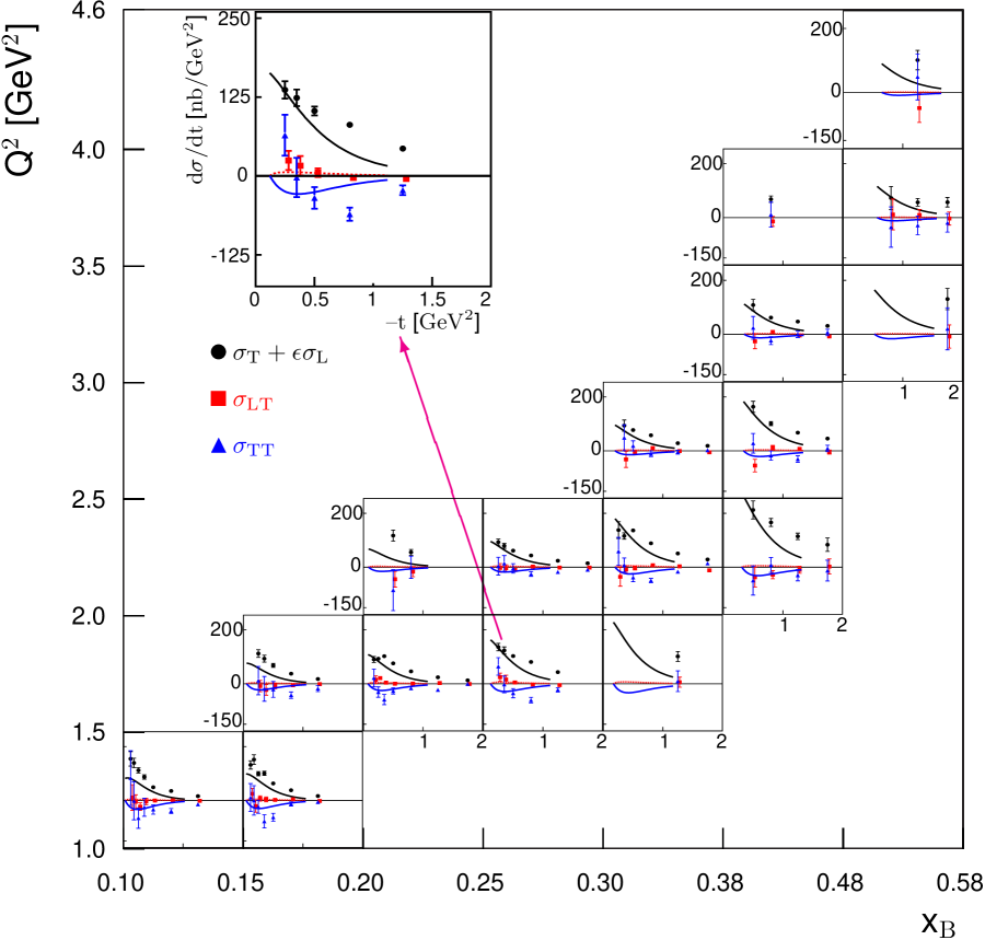
Figure 13: The structure functions vs $t$ for the different $(Q^{2},x_{B})$ bins, extracted from the present experiment. Black circules: $d\sigma_{U}/dt$. Red squares: $d\sigma_{LT}/dt$. Blue triangles: $d\sigma_{TT}/dt$. The black, red and blue curves are the corresponding results of the handbag based calculation of Ref. Goloskokov and Kroll (2011). The inset is an enlarged view of the bin with $x_{B}=0.17$ and $Q^{2}=1.87$ GeV². The error bars are statistical only.

A number of observations can be made independently of the model predictions. The $d\sigma_{TT}/dt$ structure function is negative and is smaller in magnitude than unpolarized structure function ($d\sigma_{U}/dt\equiv d\sigma_{T}/dt+\epsilon d\sigma_{L}/dt$). However, $d\sigma_{LT}/dt$ is significantly smaller than $d\sigma_{TT}/dt$. This reinforces the conclusion that the transverse photon amplitudes are dominant at the present values of $Q^{2}$.

The ratio R of the unpolarized cross sections for $\eta$ and $\pi^{0}$ for all kinematic bins is shown in Fig. 14. The ratio R is seen to be significantly less than 1, whereas the leading order handbag calculations  Eides et al. (1999) predict asymptotically $R\sim 1$. However, the observed value of R, typically about fifty percent, is greater than that predicted by the model of Ref. Goloskokov and Kroll (2011).

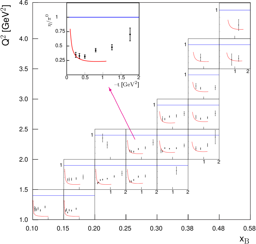
Figure 14: The ratio $R$ of the unpolarized structure functions for $\eta$ and $\pi^{0}$ extracted from the present experiment and Ref. Bedlinskiy et al. (2012), as functions of $t$ for $(Q^{2},x_{B})$ bins. The leading order handbag calculations Eides et al. (1999) predict asymptotically $R\sim 1$. The curves are the result of a handbag based calculation of Ref. Goloskokov and Kroll (2011). The inset is an enlarged view of the bin with $x_{B}=0.28$ and $Q^{2}=2.2$ GeV². The error bars are statistical only.

XI $t$- slopes

After the structure functions were obtained, fits were made to extract the $t$-dependence of $\sigma_{U}$ for different values $x_{B}$ and $Q^{2}$. For each given $x_{B}$ and $Q^{2}$ we fit this structure function with an exponential function:

$$\frac{d\sigma_{U}}{dt}=Ae^{Bt}.$$

Figure  15 shows the slope parameter $B$ as a function of $x_{B}$ for different values of $Q^{2}$. The data appear to exhibit a decrease in slope parameter with increasing $x_{B}$. However, the $Q^{2}-x_{B}$ correlation in the CLAS acceptance (see Fig. 4) does not permit one to make a definite conclusion about the $Q^{2}$ dependences of the slope parameter for fixed $x_{B}$. What one can say is that at high $Q^{2}$ and high $x_{B}$ the slope parameter appears to be smaller than for the lowest values of these variables. The $B$ parameter in the exponential determines the width of the transverse momentum distribution of the emerging protons, which, by a Fourier transform, is inversely related to the transverse size of the interaction region. From the point of view of the handbag picture, it is inversely related to the mean transverse radius of the separation between the active quark and the center of momentum of the spectators (see Ref. Burkardt (2007)). Thus the data implies that the separation is larger at the lowest $x_{B}$ and $Q^{2}$ and becomes smaller for increasing $x_{B}$ and $Q^{2}$, as it must. This is consistent with the results for $\pi^{0}$ electoproduction Bedlinskiy et al. (2014).

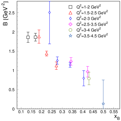
Figure 15: Slope parameters $B$ for different $x_{B}$ and $Q^{2}$ bins. The error bars are statistical only.

XII Comparisons with Theoretical Handbag Models

Figure  13 shows the experimental structure functions for bins of $Q^{2}$ and $x_{B}$. The results of the GPD-based model of Goloskokov and Kroll Goloskokov and Kroll (2011) are superimposed in Fig. 13. From these plots we conclude that the GPD-based theoretical model generally describes the CLAS data in the kinematical region of this experiment, although there are systematic discrepancies. For example, the theoretical model appears to underestimate $d\sigma_{U}/dt$ in most kinematic bins.

According to GK, the primary contributing GPDs in meson production for transverse photons are $H_{T}$, which characterizes the quark distributions involved in nucleon helicity-flip, and $\bar{E}_{T}\ (=2\widetilde{H}_{T}+E_{T}),$ which characterizes the quark distributions involved in nucleon helicity-non-flip processes Diehl and Hägler (2005); Göckeler et al. (2007). As a reminder, in both cases the active quark undergoes a helicity-flip. The GPD $\bar{E}_{T}$ is related to the spatial density of transversely polarized quarks in an unpolarized nucleon Göckeler et al. (2007).

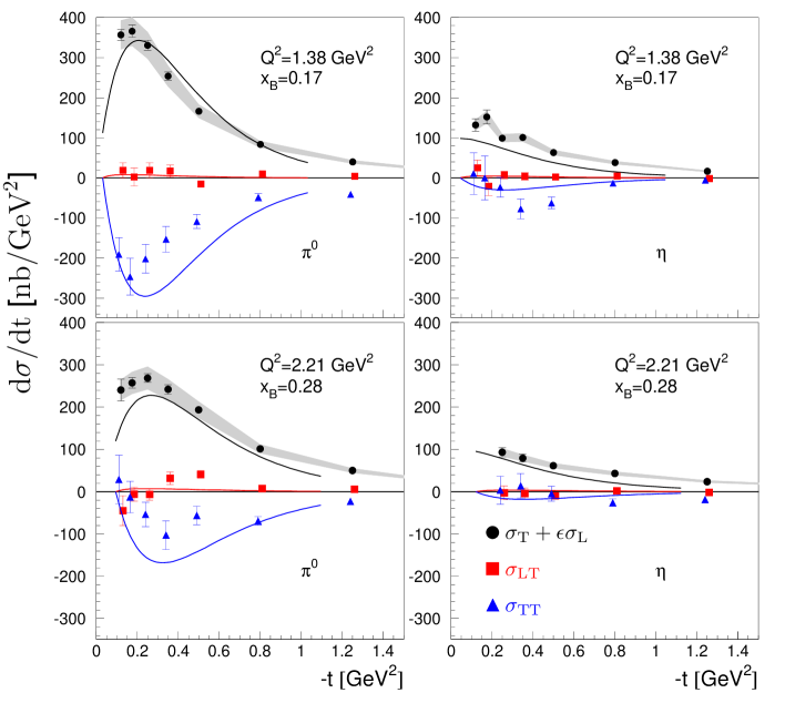
Figure 16: (Color online) The extracted structure functions vs $t$ for the $\pi^{0}$ (left column)  Olive et al. (2014) and $\eta$ (right column). The top row presents data for the kinematic point ($Q^{2}=$1.38 GeV²,$x_{B}$=0.17) and bottom row for the kinematic point ($Q^{2}=$2.21 GeV²,$x_{B}$=0.28). The data for the $\eta$ is identical to that shown in Fig. 13, with the vertical axis rescaled to highlight the difference in the magnitude of the cross sections for $\pi^{0}$ and $\eta$ electroproduction. The data and curves are as follows: black circles - $d\sigma_{U}/dt=d\sigma_{T}/dt+\epsilon d\sigma_{L}/dt$, blue triangles - $d\sigma_{TT}/dt$, red squares - $d\sigma_{LT}/dt$. The error bars are statistical only. The gray bands are our estimates of the absolute normalization systematic uncertainties on $d\sigma_{U}/dt$. The curves are theoretical predictions produced with the models of Ref. Goloskokov and Kroll (2011).

Ref. Goloskokov and Kroll (2011) obtains the following relations:

$$\begin{split}\frac{d\sigma_{T}}{dt}=&\frac{4\pi\alpha}{2k^{\prime}}\frac{\mu_{\eta}^{2}}{Q^{8}}\Bigl{[}\left(1-\xi^{2}\right)\left|\langle H_{T}\rangle\right|^{2}-\Bigl{.}\\ &\Bigr{.}\frac{t^{\prime}}{8m^{2}}\left|\langle\bar{E}_{T}\rangle\right|^{2}\Bigr{]},\end{split}$$ (9)

$$\frac{d\sigma_{TT}}{dt}=\frac{4\pi\alpha}{k^{\prime}}\frac{\mu_{\eta}^{2}}{Q^{8}}\frac{t^{\prime}}{16m^{2}}\left|\langle\bar{E}_{T}\rangle\right|^{2}.$$ (10)

Here $\kappa^{\prime}(Q^{2},x_{B})$ is a phase space factor, $t^{\prime}=t-t_{min}$, and the brackets $\langle H_{T}\rangle$ and $\langle\bar{E}_{T}\rangle$ are the Generalized Form Factors (GFFs) that denote the convolution of the elementary process with the GPDs $H_{T}$ and $\bar{E}_{T}$ (see Fig. 1).

Note that for the case of nucleon helicity-non-flip, characterized by the GPD $\bar{E}_{T}$, overall helicity from the initial to the final state is not conserved. However, angular momentum is conserved - the difference being absorbed by the orbital motion of the scattered $\eta-N$ pair. This accounts for the additional $t^{\prime}$ factor multiplying the $\bar{E}_{T}$ terms in Eqs. 9 and 10.

As in the case of $\pi^{0}$ electroproduction, the contribution of $\sigma_{L}$ accounts for only a small fraction of the unseparated structure functions $d\sigma_{U}/dt(\equiv d\sigma_{T}/dt+\epsilon d\sigma_{L}/dt)$ in the kinematic regime under investigation. This is because the contributions from $\tilde{H}$ and $\tilde{E}$ - the GPDs that are responsible for the leading-twist structure function $\sigma_{L}$ - are relatively small compared with the contributions from $\bar{E}_{T}$ and $H_{T}$ (although not quite as small for $\eta$ production as compared with $\pi^{0}$ production), which contribute to $d\sigma_{T}/dt$ and $d\sigma_{TT}/dt$. The extracted structure functions at selected values of $Q^{2}$ and $x_{B}$ for the $\pi^{0}$ (left column) and $\eta$ (right column) are shown in Fig. 16 side-by-side. The top row represents data for the kinematic point ($Q^{2}=$1.38 GeV², $x_{B}$=0.17) and the bottom row for the kinematic point ($Q^{2}=$2.21 GeV², $x_{B}$=0.28). The unpolarized structure function $d\sigma_{U}/dt$ for $\eta$ production is significantly smaller than that for $\pi^{0}$ for all measured kinematic intervals of $Q^{2},x_{B}$ and $t$. This is in contradiction to the leading order calculation  Eides et al. (1999) with $d\sigma_{L}/dt$ dominance, where the ratio is expected to be on the order of unity. In the present case, $\bar{E}_{T}$ is significantly larger than $H_{T}$. The curves in Fig. 13 and 16 are obtained by GK Goloskokov and Kroll (2011). For the GPDs, their parametrization was guided by the lattice calculation results of Ref. Göckeler et al. (2007).

The relative importance of $\bar{E}_{T}$ and $H_{T}$ can be understood by considering their composition in terms of their valence quark flavors and GPDs. Following GK, the $\pi^{0}$ and $\eta$ GPDs in terms of valence quark GPDs may be expressed as follows. For $\pi^{0}:$

$$\begin{split}H_{T}^{\pi^{0}}=(e_{u}H_{T}^{u}-e_{d}H_{T}^{d})/{\sqrt{2}},\\ \bar{E}_{T}^{\pi^{0}}=(e_{u}\bar{E}_{T}^{u}-e_{d}\bar{E}_{T}^{d})/{\sqrt{2}},\end{split}$$ (11)

where $e_{u}=1/3$ and $e_{d}=-2/3$.

For $\eta$, assuming the valence structure of the $\eta$ is purely a member of the SU(3) octet, i.e., $\eta=\eta_{8}$, and there is no contribution from strange quarks is

$$\begin{split}H_{T}^{\eta}=(e_{u}H_{T}^{u}+e_{d}H_{T}^{d})/{\sqrt{6}},\\ \bar{E}_{T}^{\eta}=(e_{u}\bar{E}_{T}^{u}+e_{d}\bar{E}_{T}^{d})/{\sqrt{6}}.\end{split}$$ (12)

In the model of GK, the sign of $H_{T}^{u}$ is positive, while the sign of $H_{T}^{d}$ is negative, but the signs of $\bar{E}_{T}^{u}$ and $\bar{E}_{T}^{d}$ are both positive. Thus, for $\pi^{0}$, taking into account the sign of $e_{u}$ and $e_{d}$, the up and down quarks enhance $\bar{E}_{T}^{\pi^{0}}$ and diminish $H_{T}^{\pi^{0}}$. The opposite effect occurs for $\eta$ mesons. By combining the $\eta$ and $\pi^{0}$ data, and Eqs. 11 and 12 above, one can estimate the GPDs of the individual valence quark flavors in the framework of the dominance of the transversity GPDs. This is currently underway Kubarovsky (2016) and will be presented later.

We further note the following features: for $\eta$ production the model of GK appears to underestimate the magnitude of $d\sigma_{U}/dt$, whereas for $\pi^{0}$ electroproduction the theoretical calculation of $d\sigma_{U}/dt$ more closely agrees with the data. Thus, one is led to the hypothesis that possibly $H_{T}$ is underestimated for $\eta$ electroproduction. Increasing $H_{T}$ will increase $d\sigma_{T}/dt$ and, therefore, $d\sigma_{U}/dt$, while not affecting $d\sigma_{TT}/dt$.

Referring again to Fig. 14, which shows the ratio of $d\sigma_{U}/dt$ for $\eta$ and $\pi^{0}$, the experimental value of this ratio is systematically higher than the theoretical prediction, which is related to the underestimation of the $\eta$ cross section.

XIII Conclusion

Differential cross sections of exclusive $\eta$ electroproduction were obtained in the few-GeV region in bins of $Q^{2},x_{B}$, $t$ and $\phi_{\eta}$. Virtual photon structure functions $d\sigma_{U}/dt=d(\sigma_{T}+\epsilon\sigma_{L})/dt$, $d\sigma_{TT}/dt$ and $d\sigma_{LT}/dt$ were extracted. It is found that $d\sigma_{U}/dt$ is larger in magnitude than $d\sigma_{TT}/dt$, while $d\sigma_{LT}/dt$ is significantly smaller than $d\sigma_{TT}/dt$. The exclusive cross sections and structure functions are typically more than a factor of two smaller than for previously measured $\pi^{0}$ electroproduction for similar kinematic intervals. It appears that some of these differences can be roughly understood from GPD-models in terms of the quark composition of $\pi^{0}$ and $\eta$ mesons. The cross section ratios of $\eta$ to $\pi^{0}$ appear to agree with the handbag calculations at low $|t|$, but show significant deviations with increasing $|t|$.

Within the handbag interpretation, there are theoretical calculations Goloskokov and Kroll (2011), which were earlier found to describe $\pi^{0}$ electroproduction Bedlinskiy et al. (2014) quite well. The result of the calculations confirmed that the measured unseparated cross sections are much larger than expected from leading-twist handbag calculations, which are dominated by longitudinal photons. For the present case, the same conclusion can be made in an almost model independent way by noting that the structure functions $d\sigma_{U}/dt$ and $d\sigma_{TT}/dt$ are significantly larger than $d\sigma_{LT}/dt$.

To make significant improvement in interpretation, higher statistical precision data, as well as $L\textrm{-}T$ separation and polarization measurements over the entire range of kinematic variables are necessary. Such experiments are planned for the Jefferson Lab operations at 12 GeV.

Appendix A Structure Functions

The structure functions are presented in Table  LABEL:strfun_table. The first error is statistical uncertainty and the second is the systematic uncertainty.

Table 5: Structure Functions

$Q^{2}$,	$x_{B}$	$-t$,	$\frac{d\sigma_{T}}{dt}+\epsilon\frac{d\sigma_{L}}{dt}$,					$\frac{d\sigma_{LT}}{dt}$,					$\frac{d\sigma_{TT}}{dt}$,
$GeV^{2}$		$GeV^{2}$	$nb/GeV^{2}$					$nb/GeV^{2}$					$nb/GeV^{2}$
1.17	0.134	0.12	$159.3$	$\pm$	$27.7$	$\pm$	$22.3$	$8.2$	$\pm$	$49.3$	$\pm$	$33.2$	$88.4$	$\pm$	$104.2$	$\pm$	$126.4$
1.17	0.134	0.17	$144.7$	$\pm$	$18.0$	$\pm$	$16.2$	$2.2$	$\pm$	$26.4$	$\pm$	$20.2$	$-4.3$	$\pm$	$73.1$	$\pm$	$189.0$
1.17	0.134	0.25	$117.3$	$\pm$	$10.3$	$\pm$	$10.7$	$-22.0$	$\pm$	$14.9$	$\pm$	$9.9$	$-71.6$	$\pm$	$40.2$	$\pm$	$29.1$
1.17	0.134	0.35	$94.0$	$\pm$	$8.8$	$\pm$	$3.6$	$-1.3$	$\pm$	$12.7$	$\pm$	$4.2$	$-29.7$	$\pm$	$35.7$	$\pm$	$9.0$
1.17	0.134	0.50	$51.1$	$\pm$	$4.3$	$\pm$	$5.9$	$1.8$	$\pm$	$6.0$	$\pm$	$4.4$	$-34.1$	$\pm$	$18.2$	$\pm$	$10.0$
1.17	0.134	0.80	$36.3$	$\pm$	$2.5$	$\pm$	$1.6$	$1.1$	$\pm$	$3.0$	$\pm$	$5.6$	$-40.6$	$\pm$	$9.5$	$\pm$	$13.3$
1.17	0.134	1.25	$16.2$	$\pm$	$1.7$	$\pm$	$1.8$	$-1.2$	$\pm$	$2.3$	$\pm$	$3.0$	$-13.7$	$\pm$	$6.2$	$\pm$	$5.0$
1.39	0.170	0.12	$134.1$	$\pm$	$15.5$	$\pm$	$21.7$	$26.2$	$\pm$	$19.8$	$\pm$	$14.2$	$15.2$	$\pm$	$52.7$	$\pm$	$27.5$
1.39	0.170	0.17	$156.4$	$\pm$	$18.2$	$\pm$	$21.9$	$-18.1$	$\pm$	$23.3$	$\pm$	$28.7$	$-0.4$	$\pm$	$56.5$	$\pm$	$8.0$
1.39	0.170	0.25	$101.8$	$\pm$	$8.0$	$\pm$	$7.9$	$10.6$	$\pm$	$10.0$	$\pm$	$6.4$	$-22.9$	$\pm$	$25.1$	$\pm$	$26.2$
1.39	0.170	0.35	$104.6$	$\pm$	$8.0$	$\pm$	$6.3$	$7.6$	$\pm$	$9.3$	$\pm$	$9.2$	$-80.1$	$\pm$	$25.3$	$\pm$	$15.4$
1.39	0.170	0.50	$65.3$	$\pm$	$4.5$	$\pm$	$2.7$	$4.3$	$\pm$	$5.0$	$\pm$	$3.1$	$-64.3$	$\pm$	$14.9$	$\pm$	$16.7$
1.39	0.170	0.80	$39.0$	$\pm$	$2.4$	$\pm$	$2.6$	$5.7$	$\pm$	$2.8$	$\pm$	$3.3$	$-11.9$	$\pm$	$8.0$	$\pm$	$4.5$
1.39	0.170	1.25	$16.9$	$\pm$	$1.5$	$\pm$	$2.1$	$-1.7$	$\pm$	$1.9$	$\pm$	$1.1$	$-6.0$	$\pm$	$5.2$	$\pm$	$2.9$
1.62	0.187	0.25	$117.1$	$\pm$	$14.6$	$\pm$	$11.6$	$-6.0$	$\pm$	$22.0$	$\pm$	$13.4$	$11.3$	$\pm$	$54.6$	$\pm$	$32.0$
1.62	0.187	0.35	$98.4$	$\pm$	$13.2$	$\pm$	$9.0$	$-20.3$	$\pm$	$20.4$	$\pm$	$6.8$	$-22.0$	$\pm$	$48.6$	$\pm$	$49.5$
1.62	0.187	0.50	$71.0$	$\pm$	$7.6$	$\pm$	$3.6$	$-5.7$	$\pm$	$10.7$	$\pm$	$6.9$	$-22.7$	$\pm$	$30.7$	$\pm$	$37.5$
1.62	0.187	0.80	$38.5$	$\pm$	$3.3$	$\pm$	$1.7$	$-4.3$	$\pm$	$4.4$	$\pm$	$2.1$	$-43.0$	$\pm$	$12.4$	$\pm$	$8.7$
1.62	0.187	1.25	$18.3$	$\pm$	$2.7$	$\pm$	$2.2$	$-1.2$	$\pm$	$3.8$	$\pm$	$1.6$	$-15.9$	$\pm$	$11.5$	$\pm$	$5.8$
1.77	0.224	0.18	$93.3$	$\pm$	$11.4$	$\pm$	$12.0$	$16.9$	$\pm$	$14.7$	$\pm$	$11.9$	$22.1$	$\pm$	$33.7$	$\pm$	$29.9$
1.77	0.224	0.25	$96.4$	$\pm$	$6.4$	$\pm$	$6.7$	$23.9$	$\pm$	$7.2$	$\pm$	$6.1$	$-30.0$	$\pm$	$20.0$	$\pm$	$14.9$
1.77	0.224	0.35	$105.0$	$\pm$	$6.6$	$\pm$	$4.1$	$7.7$	$\pm$	$7.0$	$\pm$	$6.1$	$-60.1$	$\pm$	$19.3$	$\pm$	$13.5$
1.77	0.224	0.50	$77.9$	$\pm$	$4.0$	$\pm$	$4.2$	$2.8$	$\pm$	$4.4$	$\pm$	$3.3$	$-25.4$	$\pm$	$11.7$	$\pm$	$17.3$
1.77	0.224	0.80	$46.9$	$\pm$	$2.2$	$\pm$	$3.2$	$2.1$	$\pm$	$2.4$	$\pm$	$2.1$	$-15.5$	$\pm$	$6.5$	$\pm$	$6.6$
1.77	0.224	1.25	$24.5$	$\pm$	$1.5$	$\pm$	$1.8$	$3.0$	$\pm$	$1.5$	$\pm$	$1.8$	$-22.5$	$\pm$	$4.2$	$\pm$	$2.7$
1.77	0.224	1.75	$12.9$	$\pm$	$1.7$	$\pm$	$1.5$	$-0.9$	$\pm$	$2.1$	$\pm$	$1.8$	$-0.5$	$\pm$	$4.9$	$\pm$	$4.5$
1.88	0.271	0.25	$137.5$	$\pm$	$13.8$	$\pm$	$27.9$	$27.4$	$\pm$	$15.4$	$\pm$	$19.3$	$62.5$	$\pm$	$33.0$	$\pm$	$46.8$
1.88	0.272	0.35	$125.9$	$\pm$	$13.3$	$\pm$	$11.5$	$18.9$	$\pm$	$15.3$	$\pm$	$14.7$	$-1.1$	$\pm$	$31.3$	$\pm$	$78.2$
1.88	0.271	0.50	$104.0$	$\pm$	$7.1$	$\pm$	$3.7$	$6.5$	$\pm$	$6.7$	$\pm$	$6.4$	$-34.3$	$\pm$	$17.2$	$\pm$	$31.1$
1.88	0.272	0.80	$81.9$	$\pm$	$4.7$	$\pm$	$5.1$	$-2.3$	$\pm$	$4.0$	$\pm$	$3.0$	$-60.5$	$\pm$	$10.5$	$\pm$	$10.5$
1.88	0.272	1.25	$43.6$	$\pm$	$3.4$	$\pm$	$5.6$	$-4.0$	$\pm$	$3.4$	$\pm$	$4.4$	$-23.2$	$\pm$	$7.8$	$\pm$	$7.0$
1.95	0.313	1.25	$100.9$	$\pm$	$18.2$	$\pm$	$10.3$	$6.9$	$\pm$	$18.6$	$\pm$	$18.9$	$9.5$	$\pm$	$38.4$	$\pm$	$34.7$
2.11	0.238	0.50	$121.5$	$\pm$	$21.1$	$\pm$	$10.5$	$-42.3$	$\pm$	$29.7$	$\pm$	$8.6$	$-96.2$	$\pm$	$78.9$	$\pm$	$16.2$
2.11	0.238	0.80	$55.8$	$\pm$	$10.6$	$\pm$	$6.6$	$-14.2$	$\pm$	$18.4$	$\pm$	$4.0$	$-1.4$	$\pm$	$41.5$	$\pm$	$83.4$
2.24	0.276	0.25	$97.0$	$\pm$	$11.6$	$\pm$	$10.9$	$-1.0$	$\pm$	$16.7$	$\pm$	$20.1$	$2.0$	$\pm$	$34.5$	$\pm$	$24.7$
2.24	0.276	0.35	$80.8$	$\pm$	$9.3$	$\pm$	$5.8$	$-2.0$	$\pm$	$12.9$	$\pm$	$4.7$	$15.4$	$\pm$	$29.5$	$\pm$	$15.8$
2.24	0.276	0.50	$62.5$	$\pm$	$5.3$	$\pm$	$7.3$	$-7.8$	$\pm$	$7.1$	$\pm$	$5.3$	$-5.3$	$\pm$	$18.0$	$\pm$	$25.0$
2.24	0.276	0.80	$44.1$	$\pm$	$2.8$	$\pm$	$2.3$	$3.4$	$\pm$	$3.3$	$\pm$	$2.1$	$-25.0$	$\pm$	$9.1$	$\pm$	$4.7$
2.24	0.276	1.25	$24.2$	$\pm$	$2.1$	$\pm$	$2.4$	$-1.5$	$\pm$	$2.8$	$\pm$	$2.3$	$-17.4$	$\pm$	$6.4$	$\pm$	$4.3$
2.24	0.276	1.75	$14.7$	$\pm$	$2.1$	$\pm$	$2.4$	$-1.3$	$\pm$	$2.5$	$\pm$	$2.5$	$-9.8$	$\pm$	$6.0$	$\pm$	$5.7$
2.26	0.335	0.25	$142.4$	$\pm$	$31.9$	$\pm$	$41.2$	$-35.5$	$\pm$	$35.4$	$\pm$	$49.9$	$61.6$	$\pm$	$53.2$	$\pm$	$72.7$
2.26	0.338	0.35	$116.8$	$\pm$	$11.7$	$\pm$	$7.0$	$-7.9$	$\pm$	$13.2$	$\pm$	$12.2$	$6.4$	$\pm$	$26.3$	$\pm$	$40.2$
2.26	0.338	0.50	$137.8$	$\pm$	$6.7$	$\pm$	$7.7$	$-1.9$	$\pm$	$7.1$	$\pm$	$6.4$	$-38.1$	$\pm$	$15.6$	$\pm$	$4.2$
2.26	0.338	0.80	$88.8$	$\pm$	$3.6$	$\pm$	$3.8$	$8.1$	$\pm$	$3.3$	$\pm$	$3.8$	$-49.6$	$\pm$	$7.9$	$\pm$	$6.7$
2.26	0.338	1.25	$51.2$	$\pm$	$2.7$	$\pm$	$5.5$	$3.1$	$\pm$	$2.8$	$\pm$	$6.5$	$-16.4$	$\pm$	$6.1$	$\pm$	$10.6$
2.26	0.338	1.75	$28.5$	$\pm$	$2.9$	$\pm$	$4.4$	$-11.4$	$\pm$	$3.1$	$\pm$	$6.0$	$13.7$	$\pm$	$5.1$	$\pm$	$4.6$
2.35	0.404	0.50	$215.1$	$\pm$	$34.0$	$\pm$	$19.6$	$-38.8$	$\pm$	$37.4$	$\pm$	$28.9$	$-48.3$	$\pm$	$54.3$	$\pm$	$40.4$
2.35	0.404	0.80	$165.5$	$\pm$	$14.6$	$\pm$	$19.4$	$-26.8$	$\pm$	$15.1$	$\pm$	$16.1$	$6.5$	$\pm$	$27.5$	$\pm$	$16.3$
2.35	0.404	1.25	$114.4$	$\pm$	$12.1$	$\pm$	$20.4$	$-9.7$	$\pm$	$12.9$	$\pm$	$17.9$	$-29.9$	$\pm$	$21.1$	$\pm$	$24.1$
2.35	0.404	1.75	$84.0$	$\pm$	$24.7$	$\pm$	$55.2$	$1.4$	$\pm$	$27.9$	$\pm$	$76.6$	$-12.0$	$\pm$	$38.4$	$\pm$	$100.8$
2.73	0.343	0.35	$94.2$	$\pm$	$20.7$	$\pm$	$14.9$	$-28.5$	$\pm$	$29.4$	$\pm$	$16.0$	$46.0$	$\pm$	$48.7$	$\pm$	$29.3$
2.73	0.343	0.50	$79.1$	$\pm$	$6.1$	$\pm$	$3.2$	$-3.8$	$\pm$	$8.3$	$\pm$	$6.9$	$18.8$	$\pm$	$19.3$	$\pm$	$15.1$
2.73	0.343	0.80	$58.9$	$\pm$	$3.4$	$\pm$	$2.3$	$12.5$	$\pm$	$4.3$	$\pm$	$4.4$	$-8.5$	$\pm$	$10.7$	$\pm$	$5.5$
2.73	0.343	1.25	$28.6$	$\pm$	$2.4$	$\pm$	$2.9$	$-0.2$	$\pm$	$3.2$	$\pm$	$1.2$	$-4.2$	$\pm$	$7.2$	$\pm$	$9.8$
2.73	0.343	1.75	$18.7$	$\pm$	$2.2$	$\pm$	$2.7$	$-4.8$	$\pm$	$3.0$	$\pm$	$2.4$	$2.5$	$\pm$	$6.0$	$\pm$	$9.8$
2.77	0.424	0.50	$164.4$	$\pm$	$20.7$	$\pm$	$21.0$	$-53.5$	$\pm$	$23.4$	$\pm$	$25.3$	$26.9$	$\pm$	$36.6$	$\pm$	$33.4$
2.77	0.424	0.80	$100.9$	$\pm$	$7.5$	$\pm$	$11.5$	$12.2$	$\pm$	$8.4$	$\pm$	$13.3$	$-17.2$	$\pm$	$16.9$	$\pm$	$22.4$
2.77	0.424	1.25	$67.8$	$\pm$	$5.5$	$\pm$	$7.4$	$7.9$	$\pm$	$6.4$	$\pm$	$6.1$	$-29.8$	$\pm$	$12.6$	$\pm$	$13.7$
2.77	0.424	1.75	$45.3$	$\pm$	$6.3$	$\pm$	$6.9$	$-4.4$	$\pm$	$7.6$	$\pm$	$10.3$	$9.2$	$\pm$	$11.8$	$\pm$	$17.6$
3.25	0.430	0.50	$108.4$	$\pm$	$20.7$	$\pm$	$14.8$	$-22.2$	$\pm$	$27.1$	$\pm$	$17.5$	$21.1$	$\pm$	$42.7$	$\pm$	$23.3$
3.25	0.431	0.80	$62.2$	$\pm$	$5.3$	$\pm$	$4.7$	$9.8$	$\pm$	$7.0$	$\pm$	$4.7$	$-23.3$	$\pm$	$14.8$	$\pm$	$11.9$
3.25	0.431	1.25	$47.1$	$\pm$	$4.2$	$\pm$	$3.9$	$-3.6$	$\pm$	$5.5$	$\pm$	$8.6$	$-0.6$	$\pm$	$11.8$	$\pm$	$136.3$
3.25	0.431	1.75	$30.6$	$\pm$	$4.9$	$\pm$	$3.5$	$-7.3$	$\pm$	$6.9$	$\pm$	$4.5$	$6.3$	$\pm$	$11.7$	$\pm$	$13.2$
3.30	0.497	1.75	$128.6$	$\pm$	$38.4$	$\pm$	$35.0$	$-6.8$	$\pm$	$42.0$	$\pm$	$19.6$	$17.4$	$\pm$	$77.0$	$\pm$	$52.1$
3.69	0.451	0.80	$68.1$	$\pm$	$11.7$	$\pm$	$5.9$	$-12.1$	$\pm$	$18.2$	$\pm$	$5.5$	$6.9$	$\pm$	$47.2$	$\pm$	$25.2$
3.77	0.513	0.80	$71.4$	$\pm$	$43.1$	$\pm$	$10.8$	$15.2$	$\pm$	$57.8$	$\pm$	$25.4$	$-38.8$	$\pm$	$76.2$	$\pm$	$30.0$
3.77	0.514	1.25	$56.5$	$\pm$	$14.3$	$\pm$	$7.3$	$11.5$	$\pm$	$20.2$	$\pm$	$11.1$	$-29.6$	$\pm$	$34.9$	$\pm$	$22.9$
3.77	0.513	1.75	$57.2$	$\pm$	$17.6$	$\pm$	$9.1$	$-3.4$	$\pm$	$23.9$	$\pm$	$8.8$	$-17.4$	$\pm$	$34.3$	$\pm$	$16.0$
4.24	0.540	1.25	$100.7$	$\pm$	$30.2$	$\pm$	$12.7$	$-46.3$	$\pm$	$44.9$	$\pm$	$15.4$	$48.5$	$\pm$	$72.4$	$\pm$	$20.6$

References

- Ji (1997a) X. Ji, Phys. Rev. Lett. 78, 610 (1997a).
- Ji (1997b) X. Ji, Phys. Rev. D 55, 7114 (1997b).
- Radyushkin (1996) A. V. Radyushkin, Physics Letters B 380, 417 (1996).
- Radyushkin (1997) A. V. Radyushkin, Phys. Rev. D 56, 5524 (1997).
- Hoodbhoy and Ji (1998) P. Hoodbhoy and X. Ji, Phys. Rev. D 58, 054006 (1998).
- Diehl (2003) M. Diehl, Physics Reports 388, 41 (2003).
- Bedlinskiy et al. (2012) I. Bedlinskiy, V. Kubarovsky, S. Niccolai, P. Stoler, et al. (CLAS Collaboration), Phys. Rev. Lett. 109, 112001 (2012).
- Bedlinskiy et al. (2014) I. Bedlinskiy, V. Kubarovsky, S. Niccolai, P. Stoler, et al. (CLAS Collaboration), Phys. Rev. C 90, 025205 (2014).
- Goloskokov and Kroll (2009) S. V. Goloskokov and P. Kroll, The European Physical Journal C 65, 137 (2009).
- Goloskokov and Kroll (2011) S. V. Goloskokov and P. Kroll, The European Physical Journal A 47, 112 (2011).
- Ahmad et al. (2009) S. Ahmad, G. R. Goldstein, and S. Liuti, Phys. Rev. D 79, 054014 (2009).
- Defurne et al. (2016) M. Defurne et al., Phys. Rev. Lett. 117, 262001 (2016).
- Mecking et al. (2003) B. Mecking et al., Nucl Instrum Methods Phys Res A 503, 513 (2003).
- Girod et al. (2008) F. X. Girod, R. A. Niyazov, et al. (CLAS Collaboration), Phys. Rev. Lett. 100, 162002 (2008).
- Jo et al. (2015) H. S. Jo, F. X. Girod, H. Avakian, V. D. Burkert, M. Garçon, M. Guidal, V. Kubarovsky, S. Niccolai, P. Stoler, et al. (CLAS Collaboration), Phys. Rev. Lett. 115, 212003 (2015).
- Masi et al. (2008) R. D. Masi, M. Garçon, B. Zhao, et al. (CLAS Collaboration), Phys. Rev. C 77, 042201 (2008).
- Wolin (1996) E. Wolin (CLAS Collaboration), (1996), available at ftp://ftp.jlab.org/pub/clas/doc/gsim_userguide.ps.
- Mestayer et al. (2000) M. Mestayer, D. Carman, et al., Nucl Instrum Methods Phys Res A 449, 81 (2000).
- Adams et al. (2001) G. Adams et al., Nucl Instrum Methods Phys Res A 465, 414 (2001).
- Smith et al. (1999) E. Smith et al., Nucl Instrum Methods Phys Res A 432, 265 (1999).
- Amarian et al. (2001) M. Amarian et al., Nucl Instrum Methods Phys Res A 460, 239 (2001).
- Olive et al. (2014) K. A. Olive et al. (Particle Data Group), Chin. Phys. C38, 090001 (2014).
- Hand (1963) L. N. Hand, Phys. Rev. 129, 1834 (1963).
- Bedlinskiy et al. (2016) I. Bedlinskiy et al., http://journals.aps.org/prc/abstract/10.1103/PhysRevC.95.035202 (2016).
- Mo and Tsai (1969) L. W. Mo and Y. S. Tsai, Rev. Mod. Phys. 41, 205 (1969).
- Afanasev et al. (2002) A. Afanasev, I. Akushevich, V. Burkert, and K. Joo, Phys. Rev. D 66, 074004 (2002).
- Bosted (1995) P. E. Bosted, Phys. Rev. C 51, 409 (1995).
- Christy et al. (2004) M. E. Christy et al., Phys. Rev. C 70, 015206 (2004).
- Eides et al. (1999) M. I. Eides, L. L. Frankfurt, and M. I. Strikman, Phys. Rev. D 59, 114025 (1999).
- Burkardt (2007) M. Burkardt, (2007), arXiv:0711.1881 [hep-ph] .
- Diehl and Hägler (2005) M. Diehl and P. Hägler, The European Physical Journal C 44, 87 (2005).
- Göckeler et al. (2007) M. Göckeler, P. Hägler, R. Horsley, Y. Nakamura, D. Pleiter, P. E. L. Rakow, A. Schäfer, G. Schierholz, H. Stüben, and J. M. Zanotti (QCDSF and UKQCD Collaborations), Phys. Rev. Lett. 98, 222001 (2007).
- Kubarovsky (2016) V. Kubarovsky, (2016), arXiv:1601.04367 [hep-ph] .