Learning to Generate Samples from Noise through Infusion Training

Abstract

In this work, we investigate a novel training procedure to learn a generative model as the transition operator of a Markov chain, such that, when applied repeatedly on an unstructured random noise sample, it will denoise it into a sample that matches the target distribution from the training set. The novel training procedure to learn this progressive denoising operation involves sampling from a slightly different chain than the model chain used for generation in the absence of a denoising target. In the training chain we infuse information from the training target example that we would like the chains to reach with a high probability. The thus learned transition operator is able to produce quality and varied samples in a small number of steps. Experiments show competitive results compared to the samples generated with a basic Generative Adversarial Net.

1 Introduction and motivation

To go beyond the relatively simpler tasks of classification and regression, advancing our ability to learn good generative models of high-dimensional data appears essential. There are many scenarios where one needs to efficiently produce good high-dimensional outputs where output dimensions have unknown intricate statistical dependencies: from generating realistic images, segmentations, text, speech, keypoint or joint positions, etc…, possibly as an answer to the same, other, or multiple input modalities. These are typically cases where there is not just one right answer but a variety of equally valid ones following a non-trivial and unknown distribution. A fundamental ingredient for such scenarios is thus the ability to learn a good generative model from data, one from which we can subsequently efficiently generate varied samples of high quality.

Many approaches for learning to generate high dimensional samples have been and are still actively being investigated. These approaches can be roughly classified under the following broad categories:

• Ordered visible dimension sampling (van den Oord et al., 2016; Larochelle & Murray, 2011). In this type of auto-regressive approach, output dimensions (or groups of conditionally independent dimensions) are given an arbitrary fixed ordering, and each is sampled conditionally on the previous sampled ones. This strategy is often implemented using a recurrent network (LSTM or GRU). Desirable properties of this type of strategy are that the exact log likelihood can usually be computed tractably, and sampling is exact. Undesirable properties follow from the forced ordering, whose arbitrariness feels unsatisfactory especially for domains that do not have a natural ordering (e.g. images), and imposes for high-dimensional output a long sequential generation that can be slow.

• Undirected graphical models with multiple layers of latent variables. These make inference, and thus learning, particularly hard and tend to be costly to sample from (Salakhutdinov & Hinton, 2009).

• Directed graphical models trained as variational autoencoders (VAE) (Kingma & Welling, 2014; Rezende et al., 2014)

• Adversarially-trained generative networks. (GAN)(Goodfellow et al., 2014)

• Stochastic neural networks, i.e. networks with stochastic neurons, trained by an adapted form of stochastic backpropagation

• Generative uses of denoising autoencoders (Vincent et al., 2010) and their generalization as Generative Stochastic Networks (Alain et al., 2016)

• Inverting a non-equilibrium thermodynamic slow diffusion process (Sohl-Dickstein et al., 2015)

• Continuous transformation of a distribution by invertible functions (Dinh et al. (2014), also used for variational inference in Rezende & Mohamed (2015))

Several of these approaches are based on maximizing an explicit or implicit model log-likelihood or a lower bound of its log-likelihood, but some successful ones are not e.g. GANs. The approach we propose here is based on the notion of “denoising” and thus takes its root in denoising autoencoders and the GSN type of approaches. It is also highly related to the non-equilibrium thermodynamics inverse diffusion approach of Sohl-Dickstein et al. (2015). One key aspect that distinguishes these types of methods from others listed above is that sample generation is achieved thanks to a learned stochastic mapping from input space to input space, rather than from a latent-space to input-space.

Specifically, in the present work, we propose to learn to generate high quality samples through a process of progressive, stochastic, denoising, starting from a simple initial “noise” sample generated in input space from a simple factorial distribution i.e. one that does not take into account any dependency or structure between dimensions. This, in effect, amounts to learning the transition operator of a Markov chain operating on input space. Starting from such an initial “noise” input, and repeatedly applying the operator for a small fixed number $T$ of steps, we aim to obtain a high quality resulting sample, effectively modeling the training data distribution. Our training procedure uses a novel “target-infusion” technique, designed to slightly bias model sampling to move towards a specific data point during training, and thus provide inputs to denoise which are likely under the model’s sample generation paths. By contrast with Sohl-Dickstein et al. (2015) which consists in inverting a slow and fixed diffusion process, our infusion chains make a few large jumps and follow the model distribution as the learning progresses.

The rest of this paper is structured as follows: Section 2 formally defines the model and training procedure. Section 3 discusses and contrasts our approach with the most related methods from the literature. Section 4 presents experiments that validate the approach. Section 5 concludes and proposes future work directions.

2 Proposed approach

2.1 Setup

We are given a finite data set $D$ containing $n$ points in $\mathbb{R}^{d}$, supposed drawn i.i.d from an unknown distribution $q^{*}$. The data set $D$ is supposed split into training, validation and test subsets $D_{\mathrm{train}}$, $D_{\mathrm{valid}}$, $D_{\mathrm{test}}$. We will denote $q_{\mathrm{train}}^{*}$ the empirical distribution associated to the training set, and use $\mathbf{x}$ to denote observed samples from the data set. We are interested in learning the parameters of a generative model $p$ conceived as a Markov Chain from which we can efficiently sample. Note that we are interested in learning an operator that will display fast “burn-in” from the initial factorial “noise” distribution, but beyond the initial $T$ steps we are not concerned about potential slow mixing or being stuck. We will first describe the sampling procedure used to sample from a trained model, before explaining our training procedure.

2.2 Generative model sampling procedure

The generative model $p$ is defined as the following sampling procedure:

• Using a simple factorial distribution $p^{(0)}(\mathbf{z}^{(0)})$, draw an initial sample $\mathbf{z}^{(0)}\sim p^{(0)}$, where $\mathbf{z}^{(0)}\in\mathbb{R}^{d}$. Since $p^{(0)}$ is factorial, the $d$ components of $\mathbf{z}^{(0)}$ are independent: $p^{0}$ cannot model any dependency structure. $\mathbf{z}^{(0)}$ can be pictured as essentially unstructured random noise.

• Repeatedly apply $T$ times a stochastic transition operator $p^{(t)}(\mathbf{z}^{(t)}|\mathbf{z}^{(t-1)})$, yielding a more “denoised” sample $\mathbf{z}^{(t)}\sim p^{(t)}(\mathbf{z}^{(t)}|\mathbf{z}^{(t-1)})$, where all $\mathbf{z}^{(t)}\in\mathbb{R}^{d}$.

• Output $\mathbf{z}^{(T)}$ as the final generated sample. Our generative model distribution is thus $p(\mathbf{z}^{(T)})$, the marginal associated to joint $p(\mathbf{z}^{(0)},\ldots,\mathbf{z}^{(T)})=p^{(0)}(\mathbf{z}^{(0)})~{}\left(\prod_{t=1}^{T}p^{(t)}(\mathbf{z}^{(t)}|\mathbf{z}^{(t-1)})\right)$.

In summary, samples from model $p$ are generated, starting with an initial sample from a simple distribution $p^{(0)}$, by taking the $T^{\mathrm{th}}$sample along Markov chain $\mathbf{z}^{(0)}\rightarrow\mathbf{z}^{(1)}\rightarrow\mathbf{z}^{(2)}\rightarrow\ldots\rightarrow\mathbf{z}^{(T)}$ whose transition operator is $p^{(t)}(\mathbf{z}^{(t)}|\mathbf{z}^{(t-1)})$. We will call this chain the model sampling chain. Figure 1 illustrates this sampling procedure using a model (i.e. transition operator) that was trained on MNIST. Note that we impose no formal requirement that the chain converges to a stationary distribution, as we simply read-out $\mathbf{z}^{(T)}$ as the samples from our model $p$. The chain also needs not be time-homogeneous, as highlighted by notation $p^{(t)}$ for the transitions.

The set of parameters $\theta$ of model $p$ comprise the parameters of $p^{(0)}$ and the parameters of transition operator $p^{(t)}(\mathbf{z}^{(t)}|\mathbf{z}^{(t-1)})$. For tractability, learnability, and efficient sampling, these distributions will be chosen factorial, i.e. $p^{(0)}(\mathbf{z}^{(0)})=\prod_{i=1}^{d}~{}p_{i}^{(0)}(\mathbf{z}_{i}^{(0)})$ and $p^{(t)}(\mathbf{z}^{(t)}|\mathbf{z}^{(t-1)})=\prod_{i=1}^{d}~{}p_{i}^{(t)}(\mathbf{z}_{i}^{(t)}|\mathbf{z}^{(t-1)})$. Note that the conditional distribution of an individual component $i$, $p_{i}^{(t)}(\mathbf{z}_{i}^{(t)}|\mathbf{z}^{(t-1)})$ may however be multimodal, e.g. a mixture in which case $p^{(t)}(\mathbf{z}^{(t)}|\mathbf{z}^{(t-1)})$ would be a product of independent mixtures (conditioned on $\mathbf{z}^{(t-1)}$), one per dimension. In our experiments, we will take the $p^{(t)}(\mathbf{z}^{(t)}|\mathbf{z}^{(t-1)})$ to be simple diagonal Gaussian yielding a Deep Latent Gaussian Model (DLGM) as in Rezende et al. (2014).

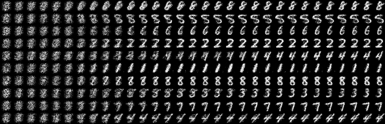
Figure 1: The model sampling chain. Each row shows a sample from $p(\mathbf{z}^{(0)},\ldots,\mathbf{z}^{(T)})$ for a model that has been trained on MNIST digits. We see how the learned Markov transition operator progressively denoises an initial unstructured noise sample. We can also see that there remains ambiguity in the early steps as to what digit this could become. This ambiguity gets resolved only in later steps. Even after a few initial steps, stochasticity could have made a chain move to a different final digit shape.

2.3 Infusion training procedure

We want to train the parameters of model $p$ such that samples from $D_{\mathrm{train}}$ are likely of being generated under the model sampling chain. Let $\theta^{(0)}$ be the parameters of $p^{(0)}$ and let $\theta^{(t)}$ be the parameters of $p^{(t)}(\mathbf{z}^{(t)}|\mathbf{z}^{(t-1)})$. Note that parameters $\theta^{(t)}$ for $t>0$ can straightforwardly be shared across time steps, which we will be doing in practice. Having committed to using (conditionally) factorial distributions for our $p^{(0)}(\mathbf{z}^{(0)})$ and $p^{(t)}(\mathbf{z}^{(t)}|\mathbf{z}^{(t-1)})$, that are both easy to learn and cheap to sample from, let us first consider the following greedy stagewise procedure. We can easily learn $p_{i}^{(0)}(\mathbf{z}^{(0)})$ to model the marginal distribution of each component $\mathbf{x}_{i}$ of the input, by training it by gradient descent on a maximum likelihood objective, i.e.

$$\theta^{(0)}=\arg\max_{\theta}~{}\mathbb{E}_{\mathbf{x}\sim q_{\mathrm{train}}^{*}}\left[\log p^{(0)}(\mathbf{x};\theta)\right]$$ (1)

This gives us a first, very crude unstructured (factorial) model of $q^{*}$.

Having learned this $p^{(0)}$, we might be tempted to then greedily learn the next stage $p^{(1)}$ of the chain in a similar fashion, after drawing samples $\mathbf{z}^{(0)}\sim p^{(0)}$ in an attempt to learn to “denoise” the sampled $\mathbf{z}^{(0)}$ into $\mathbf{x}$. Yet the corresponding following training objective $\theta^{(1)}=\arg\max_{\theta}~{}\mathbb{E}_{\mathbf{x}\sim q_{\mathrm{train}}^{*},\mathbf{z}^{(0)}\sim p^{(0)}}\left[\log p^{(1)}(\mathbf{x}|\mathbf{z}^{(0)};\theta)\right]$ makes no sense: $\mathbf{x}$ and $\mathbf{z}^{(0)}$ are sampled independently of each other so $\mathbf{z}^{(0)}$ contains no information about $\mathbf{x}$, hence $p^{(1)}(\mathbf{x}|\mathbf{z}^{(0)})=p^{(1)}(\mathbf{x})$. So maximizing this second objective becomes essentially the same as what we did when learning $p^{(0)}$. We would learn nothing more. It is essential, if we hope to learn a useful conditional distribution $p^{(1)}(\mathbf{\mathbf{\mathbf{x}}}|\mathbf{z}^{(0)})$ that it be trained on particular $\mathbf{z}^{(0)}$ containing some information about $\mathbf{x}$. In other words, we should not take our training inputs to be samples from $p^{(0)}$ but from a slightly different distribution, biased towards containing some information about $\mathbf{x}$. Let us call it $q^{(0)}(\mathbf{z}^{(0)}|\mathbf{x})$. A natural choice for it, if it were possible, would be to take $q^{(0)}(\mathbf{z}^{(0)}|\mathbf{x})=p(\mathbf{z}^{(0)}|\mathbf{z}^{(T)}=\mathbf{x})$ but this is an intractable inference, as all intermediate $\mathbf{z}^{(t)}$ between $\mathbf{z}^{(0)}$ and $\mathbf{z}^{(T)}$ are effectively latent states that we would need to marginalize over. Using a workaround such as a variational or MCMC approach would be a usual fallback. Instead, let us focus on our initial intent of guiding a progressive stochastic denoising, and think if we can come up with a different way to construct $q^{(0)}(\mathbf{z}^{(0)}|\mathbf{x})$ and similarly for the next steps $q_{i}^{(t)}(\tilde{\mathbf{z}}_{i}^{(t)}|\tilde{\mathbf{z}}^{(t-1)},\mathbf{x})$.

Eventually, we expect a sequence of samples from Markov chain $p$ to move from initial “noise” towards a specific example $\mathbf{x}$ from the training set rather than another one, primarily if a sample along the chain “resembles” $\mathbf{x}$ to some degree. This means that the transition operator should learn to pick up a minor resemblance with an $\mathbf{x}$ in order to transition to something likely to be even more similar to $\mathbf{x}$. In other words, we expect samples along a chain leading to $\mathbf{x}$ to both have high probability under the transition operator of the chain $p^{(t)}(\mathbf{z}^{(t)}|\mathbf{z}^{(t-1)})$, and to have some form of at least partial “resemblance” with $\mathbf{x}$ likely to increase as we progress along the chain. One highly inefficient way to emulate such a chain of samples would be, for teach step $t$, to sample many candidate samples from the transition operator (a conditionally factorial distribution) until we generate one that has some minimal “resemblance” to $\mathbf{x}$ (e.g. for a discrete space, this resemblance measure could be based on their Hamming distance). A qualitatively similar result can be obtained at a negligible cost by sampling from a factorial distribution that is very close to the one given by the transition operator, but very slightly biased towards producing something closer to $\mathbf{x}$. Specifically, we can “infuse” a little of $\mathbf{x}$ into our sample by choosing for each input dimension, whether we sample it from the distribution given for that dimension by the transition operator, or whether, with a small probability, we take the value of that dimension from $\mathbf{x}$. Samples from this biased chain, in which we slightly “infuse” $\mathbf{x}$, will provide us with the inputs of our input-target training pairs for the transition operator. The target part of the training pairs is simply $\mathbf{x}$.

2.3.1 The infusion chain

Formally we define an infusion chain $\widetilde{\mathbf{z}}^{(0)}\rightarrow\widetilde{\mathbf{z}}^{(1)}\rightarrow\ldots\rightarrow\widetilde{\mathbf{z}}^{(T-1)}$ whose distribution $q(\widetilde{\mathbf{z}}^{(0)},\ldots,\widetilde{\mathbf{z}}^{(T-1)}|\mathbf{x})$ will be “close” to the sampling chain $\mathbf{z}^{(0)}\rightarrow\mathbf{z}^{(1)}\rightarrow\mathbf{z}^{(2)}\rightarrow\ldots\rightarrow\mathbf{z}^{(T-1)}$ of model $p$ in the sense that $q^{(t)}(\tilde{\mathbf{z}}^{(t)}|\tilde{\mathbf{z}}^{(t-1)},\mathbf{x})$ will be close to $p^{(t)}(\mathbf{z}^{(t)}|\mathbf{z}^{(t-1)})$, but will at every step be slightly biased towards generating samples closer to target $\mathbf{x}$, i.e. $\mathbf{x}$ gets progressively “infused” into the chain. This is achieved by defining $q_{i}^{(0)}(\widetilde{\mathbf{z}}_{i}^{(0)}|\mathbf{x})$ as a mixture between $p_{i}^{(0)}$ (with a large mixture weight) and $\delta_{\mathbf{x_{i}}}$, a concentrated unimodal distribution around $\mathbf{x}_{i}$, such as a Gaussian with small variance (with a small mixture weight). Formally $q_{i}^{(0)}(\tilde{\mathbf{z}}{}_{i}^{(0)}|\mathbf{x})=(1-\alpha^{(t)})p_{i}^{(0)}(\tilde{\mathbf{z}}_{i}^{(0)})+\alpha^{(t)}\delta_{\mathbf{x_{i}}}(\tilde{\mathbf{z}}_{i}^{(0)})$, where $1-\alpha^{(t)}$ and $\alpha^{(t)}$ are the mixture weights . In other words, when sampling a value for $\tilde{\mathbf{z}}{}_{i}^{(0)}$ from $q_{i}^{(0)}$ there will be a small probability $\alpha^{(0)}$ to pick value close to $\mathbf{x}_{i}$ (as sampled from $\delta_{\mathbf{x_{i}}}$) rather than sampling the value from $p_{i}^{(0)}$. We call $\alpha^{(t)}$ the infusion rate. We define the transition operator of the infusion chain similarly as: $q_{i}^{(t)}(\tilde{\mathbf{z}}_{i}^{(t)}|\tilde{\mathbf{z}}^{(t-1)},\mathbf{x})=(1-\alpha^{(t)})p_{i}^{(t)}(\tilde{\mathbf{z}}_{i}^{(t)}|\mathbf{\tilde{\mathbf{z}}}^{(t-1)})+\alpha^{(t)}\delta_{\mathbf{x}_{i}}(\tilde{\mathbf{z}}_{i}^{(t)})$.

2.3.2 Denoising-based Infusion training procedure

For all $\mathbf{x}\in D_{\mathrm{train}}$:

• Sample from the infusion chain $\mathbf{\tilde{\mathbf{z}}}=(\tilde{\mathbf{z}}^{(0)},\ldots,\tilde{\mathbf{z}}^{(T-1)})\sim q(\tilde{\mathbf{z}}^{(0)},\ldots,\tilde{\mathbf{z}}^{(T-1)}|\mathbf{x})$.
  precisely so: $\tilde{\mathbf{z}}_{0}\sim q^{(0)}(\tilde{\mathbf{z}}^{(0)}|\mathbf{x})$  $\ldots$  $\tilde{\mathbf{z}}^{(t)}\sim q^{(t)}(\tilde{\mathbf{z}}^{(t)}|\tilde{\mathbf{z}}^{(t-1)},\mathbf{x})$   $\ldots$

• Perform a gradient step so that $p$ learns to “denoise” every $\tilde{\mathbf{z}}^{(t)}$ into $\mathbf{x}$.
  

  $$\theta^{(t)}\leftarrow\theta^{(t)}+\eta^{(t)}\frac{\partial\log p^{(t)}(\mathbf{x}|\tilde{\mathbf{z}}^{(t-1)};\theta^{(t)})}{\partial\theta^{(t)}}$$

  where $\eta^{(t)}$ is a scalar learning rate.

As illustrated in Figure 2, the distribution of samples from the infusion chain evolves as training progresses, since this chain remains close to the model sampling chain.

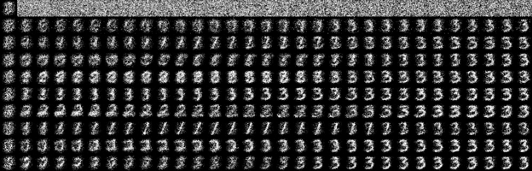
Figure 2: Training infusion chains, infused with target $\mathbf{x=}$. This figure shows the evolution of chain $q(\mathbf{z}^{(0)},\ldots,\mathbf{z}^{(30)}|\mathbf{x})$ as training on MNIST progresses. Top row is after network random weight initialization. Second row is after 1 training epochs, third after 2 training epochs, and so on. Each of these images were at a time provided as the input part of the (input, target) training pairs for the network. The network was trained to denoise all of them into target 3. We see that as training progresses, the model has learned to pick up the cues provided by target infusion, to move towards that target. Note also that a single denoising step, even with target infusion, is not sufficient for the network to produce a sharp well identified digit.

2.4 Stochastic log likelihood estimation

The exact log-likelihood of the generative model implied by our model $p$ is intractable. The log-probability of an example $\mathbf{x}$ can however be expressed using proposal distribution $q$ as:

$$\log p(\mathbf{x})=\log\mathbb{E}_{q(\widetilde{\mathbf{z}}|\mathbf{x})}\left[\frac{p(\mathbf{\tilde{\mathbf{z}}},\mathbf{x})}{q(\widetilde{\mathbf{z}}|\mathbf{x})}\right]$$ (2)

Using Jensen’s inequality we can thus derive the following lower bound:

$$\log p(\mathbf{x}) \geq \mathbb{E}_{q(\widetilde{\mathbf{z}}|\mathbf{x})}\left[\log p(\mathbf{\tilde{\mathbf{z}}},\mathbf{x})-\log q(\widetilde{\mathbf{z}}|\mathbf{x})\right]$$ (3)

where $\log p(\mathbf{\tilde{\mathbf{z}}},\mathbf{x})=\log p^{(0)}(\tilde{\mathbf{z}}^{(0)})+\left(\sum_{t=1}^{T-1}\log p^{(t)}(\tilde{\mathbf{z}}^{(t)}|\tilde{\mathbf{z}}^{(t-1)})\right)+\log p^{(T)}(\mathbf{x}|\tilde{\mathbf{z}}^{(T-1)})$ and $\log q(\mathbf{\tilde{\mathbf{z}}}|\mathbf{x})=\log q^{(0)}(\tilde{\mathbf{z}}^{(0)}|\mathbf{x})+\sum_{t=1}^{T-1}\log q^{(t)}(\tilde{\mathbf{z}}^{(t)}|\tilde{\mathbf{z}}^{(t-1)},\mathbf{x})$.

A stochastic estimation can easily be obtained by replacing the expectation by an average using a few samples from $q(\widetilde{\mathbf{z}}|\mathbf{x})$. We can thus compute a lower bound estimate of the average log likelihood over training, validation and test data.

Similarly in addition to the lower-bound based on Eq.3 we can use the same few samples from $q(\widetilde{\mathbf{z}}|\mathbf{x})$ to get an importance-sampling estimate of the likelihood based on Eq. 2.

2.4.1 Lower-bound-based infusion training procedure

Since we have derived a lower bound on the likelihood, we can alternatively choose to optimize this stochastic lower-bound directly during training. This alternative lower-bound based infusion training procedure differs only slightly from the denoising-based infusion training procedure by using $\tilde{\mathbf{z}}^{(t)}$ as a training target at step $t$ (performing a gradient step to increase $\log p^{(t)}(\tilde{\mathbf{z}}^{(t)}|\tilde{\mathbf{z}}^{(t-1)};\theta^{(t)})$) whereas denoising training always uses $\mathbf{x}$ as its target (performing a gradient step to increase $\log p^{(t)}(\mathbf{x}|\tilde{\mathbf{z}}^{(t-1)};\theta^{(t)})$). Note that the same reparametrization trick as used in Variational Auto-encoders (Kingma & Welling, 2014) can be used here to backpropagate through the chain’s Gaussian sampling.

3 Relationship to previously proposed approaches

3.1 Markov Chain Monte Carlo for energy-based models

Generating samples as a repeated application of a Markov transition operator that operates on input space is at the heart of Markov Chain Monte Carlo (MCMC) methods. They allow sampling from an energy-model, where one can efficiently compute the energy or unnormalized negated log probability (or density) at any point. The transition operator is then derived from an explicit energy function such that the Markov chain prescribed by a specific MCMC method is guaranteed to converge to the distribution defined by that energy function, as the equilibrium distribution of the chain. MCMC techniques have thus been used to obtain samples from the energy model, in the process of learning to adjust its parameters.

By contrast here we do not learn an explicit energy function, but rather learn directly a parameterized transition operator, and define an implicit model distribution based on the result of running the Markov chain.

3.2 Variational auto-encoders

Variational auto-encoders (VAE) (Kingma & Welling, 2014; Rezende et al., 2014) also start from an unstructured (independent) noise sample and non-linearly transform this into a distribution that matches the training data. One difference with our approach is that the VAE typically maps from a lower-dimensional space to the observation space. By contrast we learn a stochastic transition operator from input space to input space that we repeat for $T$ steps. Another key difference, is that the VAE learns a complex heavily parameterized approximate posterior proposal $q$ whereas our infusion based $q$ can be understood as a simple heuristic proposal distribution based on $p$. Importantly the specific heuristic we use to infuse $\mathbf{x}$ into $q$ makes sense precisely because our operator is a map from input space to input space, and couldn’t be readily applied otherwise. The generative network in Rezende et al. (2014) is a Deep Latent Gaussian Model (DLGM) just as ours. But their approximate posterior $q$ is taken to be factorial, including across all layers of the DLGM, whereas our infusion based $q$ involves an ordered sampling of the layers, as we sample from $q^{(t)}(\tilde{\mathbf{z}}^{(t)}|\tilde{\mathbf{z}}^{(t-1)},\mathbf{x})$.

More recent proposals involve sophisticated approaches to sample from better approximate posteriors, as the work of Salimans et al. (2015) in which Hamiltonian Monte Carlo is combined with variational inference, which looks very promising, though computationally expensive, and Rezende & Mohamed (2015) that generalizes the use of normalizing flows to obtain a better approximate posterior.

3.3 Sampling from autoencoders and Generative Stochastic Networks

Earlier works that propose to directly learn a transition operator resulted from research to turn autoencoder variants that have a stochastic component, in particular denoising autoencoders (Vincent et al., 2010), into generative models that one can sample from. This development is natural, since a stochastic auto-encoder is a stochastic transition operator form input space to input space. Generative Stochastic Networks (GSN) (Alain et al., 2016) generalized insights from earlier stochastic autoencoder sampling heuristics (Rifai et al., 2012) into a more formal and general framework. These previous works on generative uses of autoencoders and GSNs attempt to learn a chain whose equilibrium distribution will fit the training data. Because autoencoders and the chain are typically started from or very close to training data points, they are concerned with the chain mixing quickly between modes. By contrast our model chain is always restarted from unstructured noise, and is not required to reach or even have an equilibrium distribution. Our concern is only what happens during the $T$ “burn-in” initial steps, and to make sure that it transforms the initial factorial noise distribution into something that best fits the training data distribution. There are no mixing concerns beyond those $T$ initial steps.

A related aspect and limitation of previous denoising autoencoder and GSN approaches is that these were mainly “local” around training samples: the stochastic operator explored space starting from and primarily centered around training examples, and learned based on inputs in these parts of space only. Spurious modes in the generated samples might result from large unexplored parts of space that one might encounter while running a long chain.

3.4 Reversing a diffusion process in non-equilibrium thermodynamics

The approach of Sohl-Dickstein et al. (2015) is probably the closest to the approach we develop here. Both share a similar model sampling chain that starts from unstructured factorial noise. Neither are concerned about an equilibrium distribution. They are however quite different in several key aspects: Sohl-Dickstein et al. (2015) proceed to invert an explicit diffusion process that starts from a training set example and very slowly destroys its structure to become this random noise, they then learn to reverse this process i.e. an inverse diffusion. To maintain the theoretical argument that the exact reverse process has the same distributional form (e.g. $p(\mathbf{x}^{(t-1)}|\mathbf{x}^{(t)})$ and $p(\mathbf{x}^{(t)}|\mathbf{x}^{(t-1)})$ both factorial Gaussians), the diffusion has to be infinitesimal by construction, hence the proposed approaches uses chains with thousands of tiny steps. Instead, our aim is to learn an operator that can yield a high quality sample efficiently using only a small number $T$ of larger steps. Also our infusion training does not posit a fixed a priori diffusion process that we would learn to reverse. And while the distribution of diffusion chain samples of Sohl-Dickstein et al. (2015) is fixed and remains the same all along the training, the distribution of our infusion chain samples closely follow the model chain as our model learns. Our proposed infusion sampling technique thus adapts to the changing generative model distribution as the learning progresses.

Drawing on both Sohl-Dickstein et al. (2015) and the walkback procedure introduced for GSN in Alain et al. (2016), a variational variant of the walkback algorithm was investigated by Goyal et al. (2017) at the same time as our work. It can be understood as a different approach to learning a Markov transition operator, in which a “heating” diffusion operator is seen as a variational approximate posterior to the forward “cooling” sampling operator with the exact same form and parameters, except for a different temperature.

4 Experiments

We trained models on several datasets with real-valued examples. We used as prior distribution $p^{(0)}$ a factorial Gaussian whose parameters were set to be the mean and variance for each pixel through the training set. Similarly, our models for the transition operators are factorial Gaussians. Their mean and elementwise variance is produced as the output of a neural network that receives the previous $\mathbf{z^{(t-1)}}$ as its input, i.e. $p^{(t)}(\mathbf{z}_{i}^{(t)}|\mathbf{z}^{(t-1)})=\mathcal{N}(\mu_{i}(\mathbf{z}^{(t-1)}),\sigma_{i}^{2}(\mathbf{z}^{(t-1)}))$ where $\mu$ and $\sigma^{2}$ are computed as output vectors of a neural network. We trained such a model using our infusion training procedure on MNIST (LeCun & Cortes, 1998), Toronto Face Database (Susskind et al., 2010), CIFAR-10 (Krizhevsky & Hinton, 2009), and CelebA (Liu et al., 2015). For all datasets, the only preprocessing we did was to scale the integer pixel values down to range [0,1]. The network trained on MNIST and TFD is a MLP composed of two fully connected layers with 1200 units using batch-normalization (Ioffe & Szegedy, 2015) . The network trained on CIFAR-10 is based on the same generator as the GANs of Salimans et al. (2016), i.e. one fully connected layer followed by three transposed convolutions. CelebA was trained with the previous network where we added another transposed convolution. We use rectifier linear units (Glorot et al., 2011) on each layer inside the networks. Each of those networks have two distinct final layers with a number of units corresponding to the image size. They use sigmoid outputs, one that predict the mean and the second that predict a variance scaled by a scalar $\beta$ (In our case we chose $\beta=0.1$) and we add an epsilon $\epsilon=1e-4$ to avoid an excessively small variance. For each experiment, we trained the network on 15 steps of denoising with an increasing infusion rate of 1% ($\omega=0.01,\alpha^{{}^{(0)}}=0$), except on CIFAR-10 where we use an increasing infusion rate of 2% ($\omega=0.02,\alpha^{{}^{(0)}}=0$) on 20 steps.

4.1 Numerical results

Since we can’t compute the exact log-likelihood, the evaluation of our model is not straightforward. However we use the lower bound estimator derived in Section 2.4 to evaluate our model during training and prevent overfitting (see Figure 3). Since most previous published results on non-likelihood based models (such as GANs) used a Parzen-window-based estimator (Breuleux et al., 2011), we use it as our first comparison tool, even if it can be misleading (Lucas Theis & Bethge, 2016). Results are shown in Table 1, we use 10 000 generated samples and $\sigma=0.17$ . To get a better estimate of the log-likelihood, we then computed both the stochastic lower bound and the importance sampling estimate (IS) given in Section 2.4. For the IS estimate in our MNIST-trained model, we used 20 000 intermediates samples. In Table 1 we compare our model with the recent Annealed Importance Sampling results (Wu et al., 2016). Note that following their procedure we add an uniform noise of 1/256 to the (scaled) test point before evaluation to avoid overevaluating models that might have overfitted on the 8 bit quantization of pixel values. Another comparison tool that we used is the Inception score as in Salimans et al. (2016) which was developed for natural images and is thus most relevant for CIFAR-10. Since Salimans et al. (2016) used a GAN trained in a semi-supervised way with some tricks, the comparison with our unsupervised trained model isn’t straightforward. However, we can see in Table 2 that our model outperforms the traditional GAN trained without labeled data.

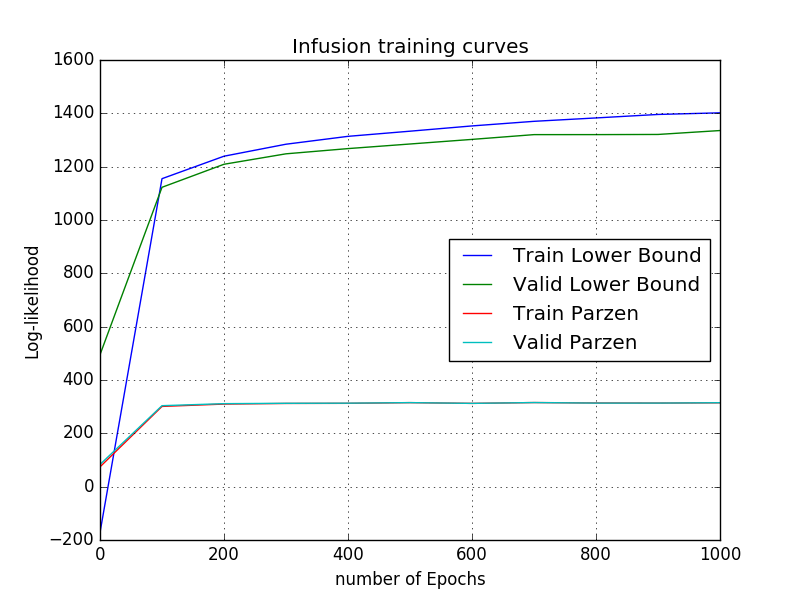
Figure 3: Training curves: lower bounds on average log-likelihood on MNIST as infusion training progresses. We also show the lower bounds estimated with the Parzen estimation method.

Model	Test
DBM (Bengio et al., 2013)	$138\pm 2$
SCAE (Bengio et al., 2013)	$121\pm 1.6$
GSN (Bengio et al., 2014)	$214\pm 1.1$
Diffusion (Sohl-Dickstein et al., 2015)	$220\pm 1.9$
GANs (Goodfellow et al.)	$225\pm 2$
GMMN + AE (Li et al.)	$282\pm 2$
Infusion training (Our)	$\mathbf{312}\pm 1.7$

Table 1: Parzen-window-based estimator of lower bound on average test log-likelihood on MNIST (in nats).

table Log-likelihood (in nats) estimated by AIS on MNIST test and training sets as reported in Wu et al. (2016) and the log likelihood estimates of our model obtained by infusion training (last three lines). Our initial model uses a Gaussian output with diagonal covariance, and we applied both our lower bound and importance sampling (IS) log-likelihood estimates to it. Since Wu et al. (2016) used only an isotropic output observation model, in order to be comparable to them, we also evaluated our model after replacing the output by an isotropic Gaussian output (same fixed variance for all pixels). Average and standard deviation over 10 repetitions of the evaluation are provided. Note that AIS might provide a higher evaluation of likelihood than our current IS estimate, but this is left for future work.

Model	Test log-likelihood (1000ex)	Train log-likelihood (100ex)
VAE-50 (AIS)	$991.435\pm 6.477$	$1272.586\pm 6.759$
GAN-50 (AIS)	$627.297\pm 8.813$	$620.498\pm 31.012$
GMMN-50 (AIS)	$593.472\pm 8.591$	$571.803\pm 30.864$
VAE-10 (AIS)	$705.375\pm 7.411$	$780.196\pm 19.147$
GAN-10 (AIS)	$328.772\pm 5.538$	$318.948\pm 22.544$
GMMN-10 (AIS)	$346.679\pm 5.860$	$345.176\pm 19.893$
Infusion training + isotropic (IS estimate)	$\mathbf{\mathrm{413.297}}\pm 0.460$	$\mathbf{\mathrm{450.695}}\pm 1.617$
Infusion training (IS estimate)	$1836.27\pm 0.551$	$1837.560\pm 1.074$
Infusion training (lower bound)	$1350.598\pm 0.079$	$1230.305\pm 0.532$

Table 2: Inception score (with standard error) of 50 000 samples generated by models trained on CIFAR-10. We use the models in Salimans et al. (2016) as baseline. ’SP’ corresponds to the best model described by Salimans et al. (2016) trained in a semi-supervised fashion. ’-L’ corresponds to the same model after removing the label in the training process (unsupervised way), ’-MBF’ corresponds to a supervised training without minibatch features.

Model	Real data	SP	-L	-MBF	Infusion training
Inception score	11.24 $\pm$ .12	8.09 $\pm$ .07	4.36 $\pm$ .06	3.87 $\pm$ .03	4.62 $\pm$ .06

4.2 Sample generation

Another common qualitative way to evaluate generative models is to look at the quality of the samples generated by the model. In Figure 4 we show various samples on each of the datasets we used. In order to get sharper images, we use at sampling time more denoising steps than in the training time (In the MNIST case we use 30 denoising steps for sampling with a model trained on 15 denoising steps). To make sure that our network didn’t learn to copy the training set, we show in the last column the nearest training-set neighbor to the samples in the next-to last column. We can see that our training method allow to generate very sharp and accurate samples on various dataset.

(a) MNIST

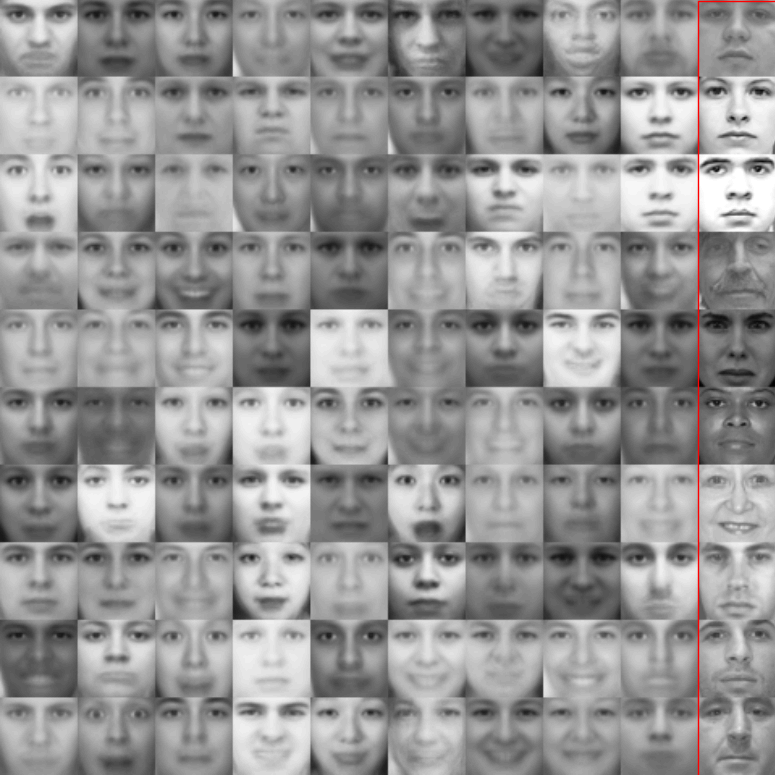
(b) Toronto Face Dataset

(c) CIFAR-10

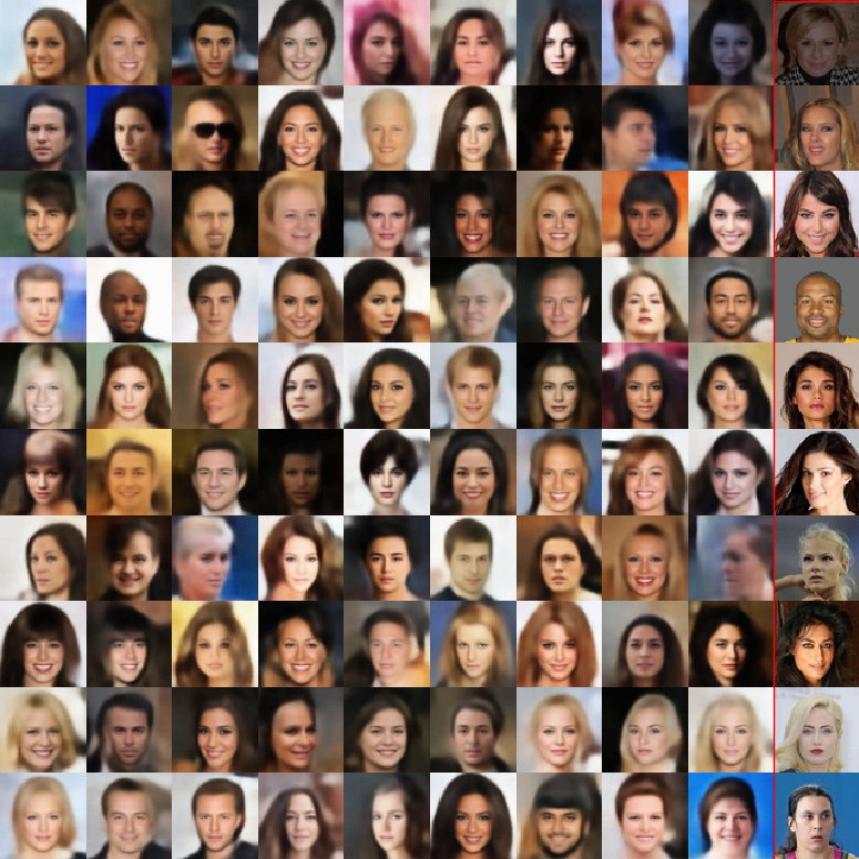
(d) CelebA

Figure 4: Mean predictions by our models on 4 different datasets. The rightmost column shows the nearest training example to the samples in the next-to last column.

4.3 Inpainting

Another method to evaluate a generative model is inpainting. It consists of providing only a partial image from the test set and letting the model generate the missing part. In one experiment, we provide only the top half of CelebA test set images and clamp that top half throughout the sampling chain. We restart sampling from our model several times, to see the variety in the distribution of the bottom part it generates. Figure 5 shows that the model is able to generate a varied set of bottom halves, all consistent with the same top half, displaying different type of smiles and expression. We also see that the generated bottom halves transfer some information about the provided top half of the images (such as pose and more or less coherent hair cut).

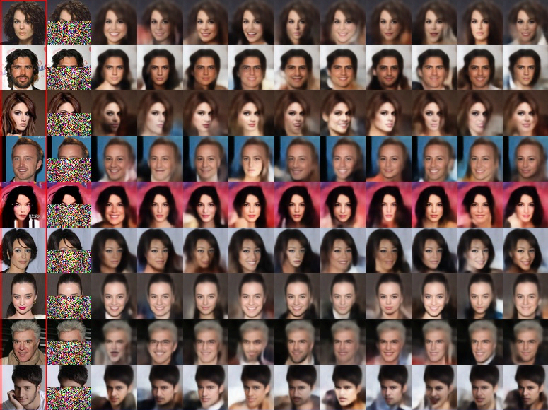
Figure 5: Inpainting on CelebA dataset. In each row, from left to right: an image form the test set; the same image with bottom half randomly sampled from our factorial prior. Then several end samples from our sampling chain in which the top part is clamped. The generated samples show that our model is able to generate a varied distribution of coherent face completions.

5 Conclusion and future work

We presented a new training procedure that allows a neural network to learn a transition operator of a Markov chain. Compared to the previously proposed method of Sohl-Dickstein et al. (2015) based on inverting a slow diffusion process, we showed empirically that infusion training requires far fewer denoising steps, and appears to provide more accurate models. Currently, many successful generative models, judged on sample quality, are based on GAN architectures. However these require to use two different networks, a generator and a discriminator, whose balance is reputed delicate to adjust, which can be source of instability during training. Our method avoids this problem by using only a single network and a simpler training objective.

Denoising-based infusion training optimizes a heuristic surrogate loss for which we cannot (yet) provide theoretical guarantees, but we empirically verified that it results in increasing log-likelihood estimates. On the other hand the lower-bound-based infusion training procedure does maximize an explicit variational lower-bound on the log-likelihood. While we have run most of our experiments with the former, we obtained similar results on the few problems we tried with lower-bound-based infusion training.

Future work shall further investigate the relationship and quantify the compromises achieved with respect to other Markov Chain methods including Sohl-Dickstein et al. (2015); Salimans et al. (2015) and also to powerful inference methods such as Rezende & Mohamed (2015). As future work, we also plan to investigate the use of more sophisticated neural net generators, similar to DCGAN’s (Radford et al., 2016) and to extend the approach to a conditional generator applicable to structured output problems.

Acknowledgments

We would like to thank the developers of Theano (Theano Development Team, 2016) for making this library available to build on, Compute Canada and Nvidia for their computation resources, NSERC and Ubisoft for their financial support, and three ICLR anonymous reviewers for helping us improve our paper.

Appendix A Details on the experiments

A.1 MNIST experiments

We show the impact of the infusion rate $\alpha^{(t)}=\alpha^{{}^{(t-1)}}+\omega$ for different numbers of training steps on the lower bound estimate of log-likelihood on the Validation set of MNIST in Figure 6. We also show the quality of generated samples and the lower bound evaluated on the test set in Table 3. Each experiment in Table 3 uses the corresponding models of Figure 6 that obtained the best lower bound value on the validation set. We use the same network architecture as described in Section 4, i.e two fully connected layers with Relu activations composed of 1200 units followed by two distinct fully connected layers composed of 784 units, one that predicts the means, the other one that predicts the variances. Each mean and variance is associated with one pixel. All of the the parameters of the model are shared across different steps except for the batch norm parameters. During training, we use the batch statistics of the current mini-batch in order to evaluate our model on the train and validation sets. At test time (Table 3), we first compute the batch statistics over the entire train set for each step and then use the computed statistics to evaluate our model on the test test.

We did some experiments to evaluate the impact of $\alpha$ or $\omega$ in $\alpha^{(t)}=\alpha^{{}^{(t-1)}}+\omega$. Figure 6 shows that as the number of steps increases, the optimal value for infusion rate decreases. Therefore, if we want to use many steps, we should have a small infusion rate. These conclusions are valid for both increasing and constant infusion rate. For example, the optimal $\alpha$ for a constant infusion rate, in Figure 6e with 10 steps is 0.08 and in Figure 6f with 15 steps is 0.06. If the number of steps is not enough or the infusion rate is too small, the network will not be able to learn the target distribution as shown in the first rows of all subsection in Table 3.

In order to show the impact of having a constant versus an increasing infusion rate, we show in Figure 7 the samples created by infused and sampling chains. We observe that having a small infusion rate over many steps ensures a slow blending of the model distribution into the target distribution.

In Table 4, we can see high lower bound values on the test set with few steps even if the model can’t generate samples that are qualitatively satisfying. These results indicate that we can’t rely on the lower bound as the only evaluation metric and this metric alone does not necessarily indicate the suitability of our model to generated good samples. However, it is still a useful tool to prevent overfitting (the networks in Figure 6e and 6f overfit when the infusion rate becomes too high). Concerning the samples quality, we observe that having a small infusion rate over an adequate number of steps leads to better samples.

(a) Networks trained with 1 infusion step. Each infusion rate in the figure corresponds to $\alpha^{(0)}$. Since we have only one step, we have $\omega=0$.

(b) Networks trained with 5 infusion steps. Each infusion rate corresponds to $\omega$. We set $\alpha^{(0)}=0$.

(c) Networks trained with 10 infusion steps. Each infusion rate corresponds to $\omega$. We set $\alpha^{(0)}=0$.

(d) Networks trained with 15 infusion steps. Each infusion rate corresponds to $\omega$. We set $\alpha^{(0)}=0$.

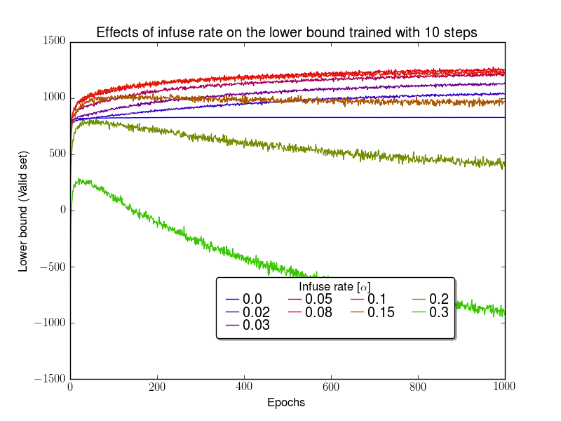
(e) Networks trained with 10 infusion steps. In this experiment we use the same infusion rate for each time step such that $\forall_{t}\alpha^{(t)}=\alpha^{(0)}$. Each infusion rate in the figure corresponds to different values for $\alpha^{(0)}$.

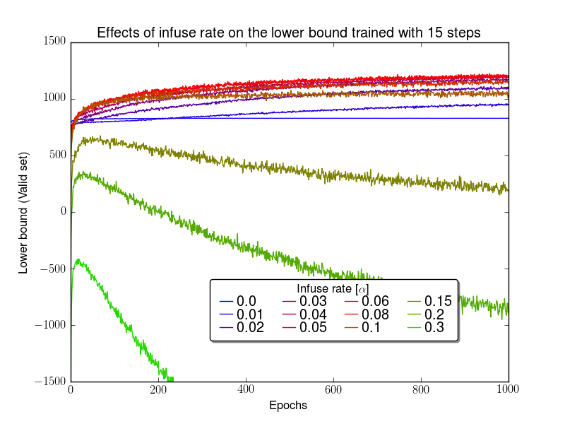
(f) Networks trained with 15 infusion steps. In this experiment we use the same infusion rate for each time step such that $\forall_{t}\alpha^{(t)}=\alpha^{(0)}$. Each infusion rate in the figure corresponds to different values $\alpha^{(0)}$.

Figure 6: Training curves on MNIST showing the log likelihood lower bound (nats) for different infusion rate schedules and different number of steps. We use an increasing schedule $\alpha^{(t)}=\alpha^{{}^{(t-1)}}+\omega$. In each sub-figure for a fixed number of steps, we show the lower bound for different infusion rates.

Table 3: Infusion rate impact on the lower bound log-likelihood (test set) and the samples generated by a network trained with different number of steps. Each sub-table corresponds to a fixed number of steps. Each row corresponds to a different infusion rate, where we show its lower bound and also its corresponding generated samples from the trained model. Note that for images, we show the mean of the Gaussian distributions instead of the true samples. As the number of steps increases, the optimal infusion rate decreases. Higher number of steps contributes to better qualitative samples, as the best samples can be seen with 15 steps using $\alpha=0.01$.

infusion rate	Lower bound (test)	Means of the model
0.0	824.34
0.05	885.35
0.1	967.25
0.15	1063.27
0.2	1115.15
0.25	1158.81
$\mathbf{0.3}$	$\mathbf{1209.39}$
0.4	1209.16
0.5	1132.05
0.6	1008.60
0.7	854.40
0.9	-161.37

(a) infusion rate impact on the lower bound log-likelihood (test set) and the samples generated by a network trained with 1 step.

infusion rate	Lower bound (test)
0.0	823.81
0.01	910.19
0.03	1142.43
0.05	1303.19
0.08	1406.38
$\mathbf{0.1}$	$\mathbf{1448.66}$
0.15	1397.41
0.2	1262.57

(b) infusion rate impact on the lower bound log-likelihood (test set) and the samples generated by a network trained with 5 steps

infusion rate	Lower bound (test)
0.0	824.42
0.01	1254.07
$\mathbf{0.02}$	$\mathbf{1389.12}$
0.03	$1366.6$8
0.04	1223.47
0.05	1057.43
0.05	846.73
0.07	658.66

(c) infusion rate impact on the lower bound log-likelihood (test set) and the samples generated by a network trained with 10 steps

infusion rate	Lower bound (test)
0.0	824.50
$\mathbf{0.01}$	$\mathbf{1351.03}$
0.02	1066.60
0.03	609.10
0.04	876.93
0.05	-479.69
0.06	-941.78

(d) infusion rate impact on the lower bound log-likelihood (test set) and the samples generated by a network trained with 15 steps

(a) Chains infused with MNIST test set samples by a constant rate ($\alpha^{(0)}=0.05,\enskip\omega=0$) in 15 steps.

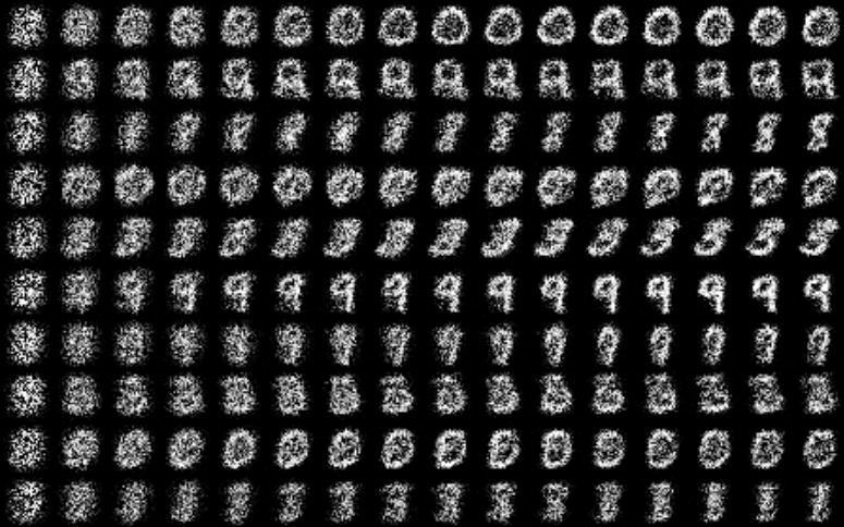
(b) Model sampling chains on MNIST using a network trained with a constant infusion rate ($\alpha^{(0)}=0.05,\enskip\omega=0$) in 15 steps.

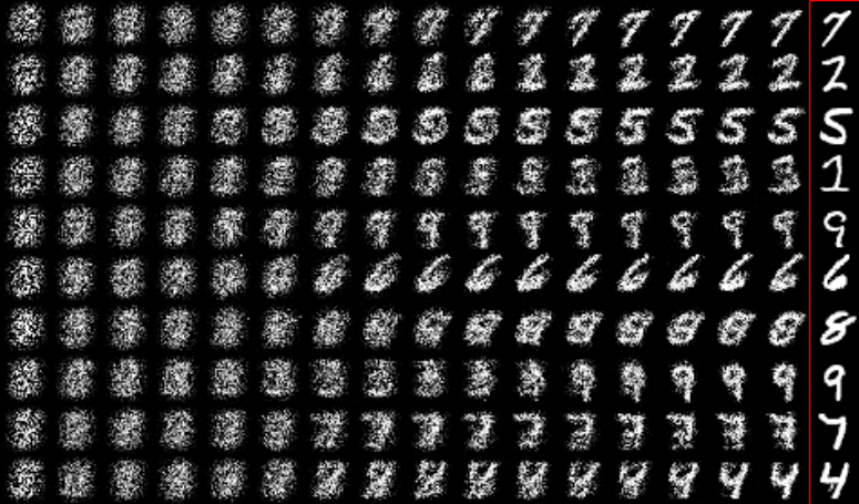
(c) Chains infused with MNIST test set samples by an increasing rate ($\alpha^{(0)}=0.0,\enskip\omega=0.01$) in 15 steps.

(d) Model sampling chains on MNIST using a network trained with an increasing infusion rate ($\alpha^{(0)}=0.0,\enskip\omega=0.01$) in 15 steps.

Figure 7: Comparing samples of constant infusion rate versus an increasing infusion rate on infused and generated chains. The models are trained on MNIST in 15 steps. Note that having an increasing infusion rate with a small value for $\omega$ allows a slow convergence to the target distribution. In contrast having a constant infusion rate leads to a fast convergence to a specific point. Increasing infusion rate leads to more visually appealing samples. We observe that having an increasing infusion rate over many steps ensures a slow blending of the model distribution into the target distribution.

A.2 Infusion and model sampling chains on natural images datasets

In order to show the behavior of our model trained by Infusion on more complex datasets, we show in Figure 8 chains on CIFAR-10 dataset and in Figure 9 chains on CelebA dataset. In each Figure, the first sub-figure shows the chains infused by some test examples and the second sub-figure shows the model sampling chains. In the experiment on CIFAR-10, we use an increasing schedule $\alpha^{(t)}=\alpha^{{}^{(t-1)}}+0.02$ with $\alpha^{(0)}=0$ and 20 infusion steps (this corresponds to the training parameters). In the experiment on CelebA, we use an increasing schedule $\alpha^{(t)}=\alpha^{{}^{(t-1)}}+0.01$ with $\alpha^{(0)}=0$ and 15 infusion steps.

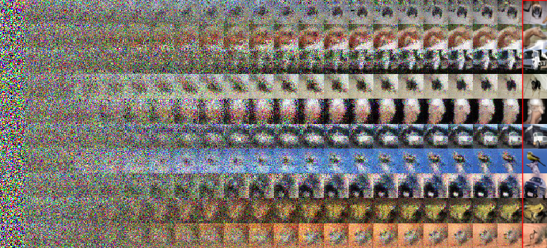
(a) Infusion chains on CIFAR-10. Last column corresponds to the target used to infuse the chain.

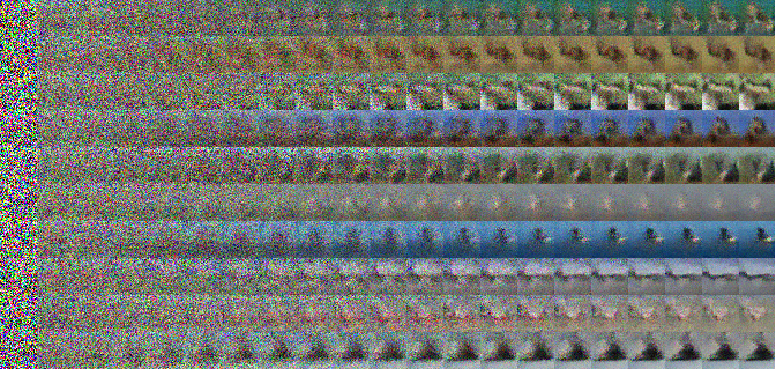
(b) Model sampling chains on CIFAR-10

Figure 8: Infusion chains (Sub-Figure 8a) and model sampling chains (Sub-Figure 8b) on CIFAR-10.

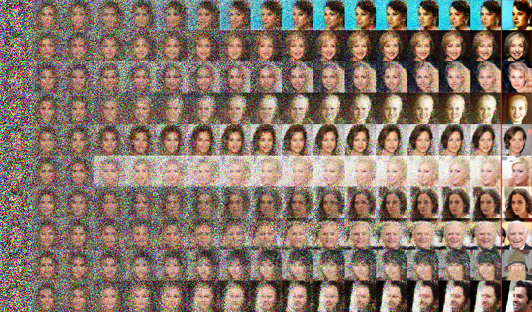
(a) Infusion chains on CelebA. Last column corresponds to the target used to infuse the chain.

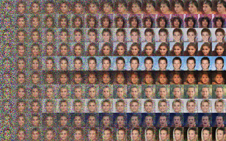
(b) Model sampling chains on CelebA

Figure 9: Infusion chains (Sub-Figure 9a) and model sampling chains (Sub-Figure 9b) on CelebA.

References

- Alain et al. (2016) Guillaume Alain, Yoshua Bengio, Li Yao, Jason Yosinski, Eric Thibodeau-Laufer, Saizheng Zhang, and Pascal Vincent. GSNs: generative stochastic networks. Information and Inference, 2016. doi: 10.1093/imaiai/iaw003.
- Bengio et al. (2013) Yoshua Bengio, Grégoire Mesnil, Yann Dauphin, and Salah Rifai. Better mixing via deep representations. In Proceedings of the 30th International Conference on Machine Learning (ICML 2013), 2013.
- Bengio et al. (2014) Yoshua Bengio, Eric Laufer, Guillaume Alain, and Jason Yosinski. Deep generative stochastic networks trainable by backprop. In Proceedings of the 31st International Conference on Machine Learning (ICML 2014), pp. 226–234, 2014.
- Breuleux et al. (2011) Olivier Breuleux, Yoshua Bengio, and Pascal Vincent. Quickly generating representative samples from an rbm-derived process. Neural Computation, 23(8):2058–2073, 2011.
- Dinh et al. (2014) Laurent Dinh, David Krueger, and Yoshua Bengio. Nice: Non-linear independent components estimation. arXiv preprint arXiv:1410.8516, 2014.
- Glorot et al. (2011) Xavier Glorot, Antoine Bordes, and Yoshua Bengio. Deep sparse rectifier neural networks. In Aistats, volume 15, pp. 275, 2011.
- Goodfellow et al. (2014) Ian Goodfellow, Jean Pouget-Abadie, Mehdi Mirza, Bing Xu, David Warde-Farley, Sherjil Ozair, Aaron Courville, and Yoshua Bengio. Generative adversarial nets. In Z. Ghahramani, M. Welling, C. Cortes, N. D. Lawrence, and K. Q. Weinberger (eds.), Advances in Neural Information Processing Systems 27, pp. 2672–2680. Curran Associates, Inc., 2014.
- Goyal et al. (2017) Anirudh Goyal, Nan Rosemary Ke, Alex Lamb, and Yoshua Bengio. The variational walkback algorithm. Technical report, Université de Montréal, 2017. URL https://openreview.net/forum?id=rkpdnIqlx. On openreview.net.
- Ioffe & Szegedy (2015) Sergey Ioffe and Christian Szegedy. Batch normalization: Accelerating deep network training by reducing internal covariate shift. Proceedings of The 32nd International Conference on Machine Learning, pp. 448–456, 2015.
- Kingma & Welling (2014) Diederik P Kingma and Max Welling. Auto-encoding variational bayes. In Proceedings of the 2nd International Conference on Learning Representations (ICLR 2014), 2014.
- Krizhevsky & Hinton (2009) Alex. Krizhevsky and Geoffrey E Hinton. Learning multiple layers of features from tiny images. Master’s thesis, Department of Computer Science, University of Toronto, 2009.
- Larochelle & Murray (2011) Hugo Larochelle and Iain Murray. The neural autoregressive distribution estimator. In AISTATS, volume 1, pp. 2, 2011.
- LeCun & Cortes (1998) Yann LeCun and Corinna Cortes. The mnist database of handwritten digits, 1998.
- Li et al. (2015) Yujia Li, Kevin Swersky, and Richard Zemel. Generative moment matching networks. In International Conference on Machine Learning (ICML 2015), pp. 1718–1727, 2015.
- Liu et al. (2015) Ziwei Liu, Ping Luo, Xiaogang Wang, and Xiaoou Tang. Deep learning face attributes in the wild. In Proceedings of International Conference on Computer Vision (ICCV 2015), December 2015.
- Lucas Theis & Bethge (2016) Aäron van den Oord Lucas Theis and Matthias Bethge. A note on the evaluation of generative models. In Proceedings of the 4th International Conference on Learning Representations (ICLR 2016), 2016.
- Radford et al. (2016) Alec Radford, Luke Metz, and Soumith Chintala. Unsupervised representation learning with deep convolutional generative adversarial networks. International Conference on Learning Representations, 2016.
- Rezende & Mohamed (2015) Danilo Rezende and Shakir Mohamed. Variational inference with normalizing flows. In Proceedings of the 32nd International Conference on Machine Learning (ICML 2015), pp. 1530–1538, 2015.
- Rezende et al. (2014) Danilo Jimenez Rezende, Shakir Mohamed, and Daan Wierstra. Stochastic backpropagation and approximate inference in deep generative models. In Proceedings of the 31th International Conference on Machine Learning, ICML 2014, Beijing, China, 21-26 June 2014, pp. 1278–1286, 2014. URL http://jmlr.org/proceedings/papers/v32/rezende14.html.
- Rifai et al. (2012) Salah Rifai, Yoshua Bengio, Yann Dauphin, and Pascal Vincent. A generative process for sampling contractive auto-encoders. In Proceedings of the 29th International Conference on Machine Learning (ICML 2012), 2012.
- Salakhutdinov & Hinton (2009) Ruslan Salakhutdinov and Geoffrey E Hinton. Deep boltzmann machines. In AISTATS, volume 1, pp. 3, 2009.
- Salimans et al. (2015) Tim Salimans, Diederik Kingma, and Max Welling. Markov chain monte carlo and variational inference: Bridging the gap. In Proceedings of The 32nd International Conference on Machine Learning, pp. 1218–1226, 2015.
- Salimans et al. (2016) Tim Salimans, Ian J. Goodfellow, Wojciech Zaremba, Vicki Cheung, Alec Radford, and Xi Chen. Improved techniques for training gans. CoRR, abs/1606.03498, 2016.
- Sohl-Dickstein et al. (2015) Jascha Sohl-Dickstein, Eric A. Weiss, Niru Maheswaranathan, and Surya Ganguli. Deep Unsupervised Learning using Nonequilibrium Thermodynamics. In Proceedings of the 32nd International Conference on Machine Learning, volume 37 of JMLR Proceedings, pp. 2256–2265. JMLR.org, 2015.
- Susskind et al. (2010) Josh M Susskind, Adam K Anderson, and Geoffrey E Hinton. The toronto face database. Department of Computer Science, University of Toronto, Toronto, ON, Canada, Tech. Rep, 3, 2010.
- Theano Development Team (2016) Theano Development Team. Theano: A Python framework for fast computation of mathematical expressions. arXiv e-prints, abs/1605.02688, may 2016.
- van den Oord et al. (2016) Aäron van den Oord, Nal Kalchbrenner, and Koray Kavukcuoglu. Pixel recurrent neural networks. In Proceedings of the 33nd International Conference on Machine Learning (ICML 2016), pp. 1747–1756, 2016.
- Vincent et al. (2010) Pascal Vincent, Hugo Larochelle, Isabelle Lajoie, Yoshua Bengio, and Pierre-Antoine Manzagol. Stacked denoising autoencoders: Learning useful representations in a deep network with a local denoising criterion. Journal of Machine Learning Research, 11(Dec):3371–3408, 2010.
- Wu et al. (2016) Yuhuai Wu, Yuri Burda, Ruslan Salakhutdinov, and Roger B. Grosse. On the quantitative analysis of decoder-based generative models. CoRR, abs/1611.04273, 2016.