Daily monitoring of TeV gamma-ray emission from Mrk 421, Mrk 501, and the Crab Nebula with HAWC

A.U. Abeysekara Department of Physics and Astronomy, University of Utah, Salt Lake City, UT, USA A. Albert Physics Division, Los Alamos National Laboratory, Los Alamos, NM, USA R. Alfaro Instituto de Física, Universidad Nacional Autónoma de México, Mexico City, Mexico C. Alvarez Universidad Autónoma de Chiapas, Tuxtla Gutiérrez, Chiapas, México J.D. Álvarez Universidad Michoacana de San Nicolás de Hidalgo, Morelia, Mexico R. Arceo Universidad Autónoma de Chiapas, Tuxtla Gutiérrez, Chiapas, México J.C. Arteaga-Velázquez Universidad Michoacana de San Nicolás de Hidalgo, Morelia, Mexico D. Avila Rojas Instituto de Física, Universidad Nacional Autónoma de México, Mexico City, Mexico H.A. Ayala Solares Department of Physics, Michigan Technological University, Houghton, MI, USA A.S. Barber Department of Physics and Astronomy, University of Utah, Salt Lake City, UT, USA N. Bautista-Elivar Universidad Politecnica de Pachuca, Pachuca, Hidalgo, Mexico J. Becerra Gonzalez NASA Goddard Space Flight Center, Greenbelt, MD, USA A. Becerril Instituto de Física, Universidad Nacional Autónoma de México, Mexico City, Mexico E. Belmont-Moreno Instituto de Física, Universidad Nacional Autónoma de México, Mexico City, Mexico S.Y. BenZvi Department of Physics & Astronomy, University of Rochester, Rochester, NY , USA A. Bernal Instituto de Astronomía, Universidad Nacional Autónoma de México, Mexico City, Mexico J. Braun Department of Physics, University of Wisconsin-Madison, Madison, WI, USA C. Brisbois Department of Physics, Michigan Technological University, Houghton, MI, USA K.S. Caballero-Mora Universidad Autónoma de Chiapas, Tuxtla Gutiérrez, Chiapas, México T. Capistrán Instituto Nacional de Astrofísica, Óptica y Electrónica, Puebla, Mexico A. Carramiñana Instituto Nacional de Astrofísica, Óptica y Electrónica, Puebla, Mexico S. Casanova Instytut Fizyki Jadrowej im Henryka Niewodniczanskiego Polskiej Akademii Nauk, Krakow, Poland M. Castillo Universidad Michoacana de San Nicolás de Hidalgo, Morelia, Mexico U. Cotti Universidad Michoacana de San Nicolás de Hidalgo, Morelia, Mexico J. Cotzomi Facultad de Ciencias Físico Matemáticas, Benemérita Universidad Autónoma de Puebla, Puebla, Mexico S. Coutiño de León Instituto Nacional de Astrofísica, Óptica y Electrónica, Puebla, Mexico C. De León Facultad de Ciencias Físico Matemáticas, Benemérita Universidad Autónoma de Puebla, Puebla, Mexico E. De la Fuente Departamento de Física, Centro Universitario de Ciencias Exactas e Ingenierías, Universidad de Guadalajara, Guadalajara, Mexico R. Diaz Hernandez Instituto Nacional de Astrofísica, Óptica y Electrónica, Puebla, Mexico B.L. Dingus Physics Division, Los Alamos National Laboratory, Los Alamos, NM, USA M.A. DuVernois Department of Physics, University of Wisconsin-Madison, Madison, WI, USA J.C. Díaz-Vélez Departamento de Física, Centro Universitario de Ciencias Exactas e Ingenierías, Universidad de Guadalajara, Guadalajara, Mexico R.W. Ellsworth School of Physics, Astronomy, and Computational Sciences, George Mason University, Fairfax, VA, USA K. Engel Department of Physics, University of Maryland, College Park, MD, USA D.W. Fiorino Department of Physics, University of Maryland, College Park, MD, USA N. Fraija Instituto de Astronomía, Universidad Nacional Autónoma de México, Mexico City, Mexico J.A. García-González Instituto de Física, Universidad Nacional Autónoma de México, Mexico City, Mexico F. Garfias Instituto de Astronomía, Universidad Nacional Autónoma de México, Mexico City, Mexico M. Gerhardt Department of Physics, Michigan Technological University, Houghton, MI, USA A. González Muñoz Instituto de Física, Universidad Nacional Autónoma de México, Mexico City, Mexico M.M. González Instituto de Astronomía, Universidad Nacional Autónoma de México, Mexico City, Mexico J.A. Goodman Department of Physics, University of Maryland, College Park, MD, USA Z. Hampel-Arias Department of Physics, University of Wisconsin-Madison, Madison, WI, USA J.P. Harding Physics Division, Los Alamos National Laboratory, Los Alamos, NM, USA S. Hernandez Instituto de Física, Universidad Nacional Autónoma de México, Mexico City, Mexico A. Hernandez-Almada Instituto de Física, Universidad Nacional Autónoma de México, Mexico City, Mexico B. Hona Department of Physics, Michigan Technological University, Houghton, MI, USA C.M. Hui NASA Marshall Space Flight Center, Astrophysics Office, Huntsville, AL, USA P. Hüntemeyer Department of Physics, Michigan Technological University, Houghton, MI, USA A. Iriarte Instituto de Astronomía, Universidad Nacional Autónoma de México, Mexico City, Mexico A. Jardin-Blicq Max-Planck Institute for Nuclear Physics, Heidelberg, Germany V. Joshi Max-Planck Institute for Nuclear Physics, Heidelberg, Germany S. Kaufmann Universidad Autónoma de Chiapas, Tuxtla Gutiérrez, Chiapas, México D. Kieda Department of Physics and Astronomy, University of Utah, Salt Lake City, UT, USA A. Lara Instituto de Geofísica, Universidad Nacional Autónoma de México, Mexico City, Mexico R.J. Lauer Department of Physics and Astronomy, University of New Mexico, Albuquerque, NM, USA W.H. Lee Instituto de Astronomía, Universidad Nacional Autónoma de México, Mexico City, Mexico D. Lennarz School of Physics and Center for Relativistic Astrophysics - Georgia Institute of Technology, Atlanta, GA, USA H. León Vargas Instituto de Física, Universidad Nacional Autónoma de México, Mexico City, Mexico J.T. Linnemann Department of Physics and Astronomy, Michigan State University, East Lansing, MI, USA A.L. Longinotti Instituto Nacional de Astrofísica, Óptica y Electrónica, Puebla, Mexico G. Luis Raya Universidad Politecnica de Pachuca, Pachuca, Hidalgo, Mexico R. Luna-García Centro de Investigación en Computación, Instituto Politécnico Nacional, Mexico City, Mexico. R. López-Coto Max-Planck Institute for Nuclear Physics, Heidelberg, Germany K. Malone Department of Physics, Pennsylvania State University, University Park, PA, USA S.S. Marinelli Department of Physics and Astronomy, Michigan State University, East Lansing, MI, USA O. Martinez Facultad de Ciencias Físico Matemáticas, Benemérita Universidad Autónoma de Puebla, Puebla, Mexico I. Martinez-Castellanos Department of Physics, University of Maryland, College Park, MD, USA J. Martínez-Castro Centro de Investigación en Computación, Instituto Politécnico Nacional, Mexico City, Mexico. J.A. Matthews Department of Physics and Astronomy, University of New Mexico, Albuquerque, NM, USA P. Miranda-Romagnoli Universidad Autónoma del Estado de Hidalgo, Pachuca, Mexico E. Moreno Facultad de Ciencias Físico Matemáticas, Benemérita Universidad Autónoma de Puebla, Puebla, Mexico M. Mostafá Department of Physics, Pennsylvania State University, University Park, PA, USA L. Nellen Instituto de Ciencias Nucleares, Universidad Nacional Autónoma de México, Mexico City, Mexico M. Newbold Department of Physics and Astronomy, University of Utah, Salt Lake City, UT, USA M.U. Nisa Department of Physics & Astronomy, University of Rochester, Rochester, NY , USA R. Noriega-Papaqui Universidad Autónoma del Estado de Hidalgo, Pachuca, Mexico J. Pretz Department of Physics, Pennsylvania State University, University Park, PA, USA E.G. Pérez-Pérez Universidad Politecnica de Pachuca, Pachuca, Hidalgo, Mexico Z. Ren Department of Physics and Astronomy, University of New Mexico, Albuquerque, NM, USA C.D. Rho Department of Physics & Astronomy, University of Rochester, Rochester, NY , USA C. Rivière Department of Physics, University of Maryland, College Park, MD, USA D. Rosa-González Instituto Nacional de Astrofísica, Óptica y Electrónica, Puebla, Mexico M. Rosenberg Department of Physics, Pennsylvania State University, University Park, PA, USA E. Ruiz-Velasco Instituto de Física, Universidad Nacional Autónoma de México, Mexico City, Mexico F. Salesa Greus Instytut Fizyki Jadrowej im Henryka Niewodniczanskiego Polskiej Akademii Nauk, Krakow, Poland A. Sandoval Instituto de Física, Universidad Nacional Autónoma de México, Mexico City, Mexico M. Schneider Santa Cruz Institute for Particle Physics, University of California, Santa Cruz, Santa Cruz, CA, USA H. Schoorlemmer Max-Planck Institute for Nuclear Physics, Heidelberg, Germany G. Sinnis Physics Division, Los Alamos National Laboratory, Los Alamos, NM, USA A.J. Smith Department of Physics, University of Maryland, College Park, MD, USA R.W. Springer Department of Physics and Astronomy, University of Utah, Salt Lake City, UT, USA P. Surajbali Max-Planck Institute for Nuclear Physics, Heidelberg, Germany I. Taboada School of Physics and Center for Relativistic Astrophysics - Georgia Institute of Technology, Atlanta, GA, USA O. Tibolla Universidad Autónoma de Chiapas, Tuxtla Gutiérrez, Chiapas, México K. Tollefson Department of Physics and Astronomy, Michigan State University, East Lansing, MI, USA I. Torres Instituto Nacional de Astrofísica, Óptica y Electrónica, Puebla, Mexico T.N. Ukwatta Physics Division, Los Alamos National Laboratory, Los Alamos, NM, USA G. Vianello Department of Physics, Stanford University, Stanford, CA, USA T. Weisgarber Department of Physics, University of Wisconsin-Madison, Madison, WI, USA S. Westerhoff Department of Physics, University of Wisconsin-Madison, Madison, WI, USA I.G. Wisher Department of Physics, University of Wisconsin-Madison, Madison, WI, USA J. Wood Department of Physics, University of Wisconsin-Madison, Madison, WI, USA T. Yapici Department of Physics and Astronomy, Michigan State University, East Lansing, MI, USA P.W. Younk Physics Division, Los Alamos National Laboratory, Los Alamos, NM, USA A. Zepeda Physics Department, Centro de Investigacion y de Estudios Avanzados del IPN, Mexico City, Mexico H. Zhou Physics Division, Los Alamos National Laboratory, Los Alamos, NM, USA

Abstract

We present results from daily monitoring of gamma rays in the energy range $\sim 0.5$ to $\sim 100$ TeV with the first 17 months of data from the High Altitude Water Cherenkov (HAWC) Observatory. Its wide field of view of 2 steradians and duty cycle of $>95$ % are unique features compared to other TeV observatories that allow us to observe every source that transits over HAWC for up to $\sim 6$ hours each sidereal day. This regular sampling yields unprecedented light curves from unbiased measurements that are independent of seasons or weather conditions. For the Crab Nebula as a reference source we find no variability in the TeV band. Our main focus is the study of the TeV blazars Markarian (Mrk) 421 and Mrk 501. A spectral fit for Mrk 421 yields a power law index $\Gamma=2.21\pm 0.14_{\mathrm{stat}}\pm 0.20_{\mathrm{sys}}$ and an exponential cut-off $E_{0}=5.4\pm 1.1_{\mathrm{stat}}\pm 1.0_{\mathrm{sys}}$ TeV. For Mrk 501, we find an index $\Gamma=1.60\pm 0.30_{\mathrm{stat}}\pm 0.20_{\mathrm{sys}}$ and exponential cut-off $E_{0}=5.7\pm 1.6_{\mathrm{stat}}\pm 1.0_{\mathrm{sys}}$ TeV. The light curves for both sources show clear variability and a Bayesian analysis is applied to identify changes between flux states. The highest per-transit fluxes observed from Mrk 421 exceed the Crab Nebula flux by a factor of approximately five. For Mrk 501, several transits show fluxes in excess of three times the Crab Nebula flux. In a comparison to lower energy gamma-ray and X-ray monitoring data with comparable sampling we cannot identify clear counterparts for the most significant flaring features observed by HAWC.

gamma rays: observations, galaxies: active, BL Lacertae objects: individual (Mrk 421, Mrk 501), ISM: individual (Crab Nebula), acceleration of particles

^†^†software: 3ML (Vianello et al., 2016), HEALPix (Gorski et al., 2005), ROOT (Brun & Rademakers, 1997), NumPy and SciPy (van der Walt et al., 2011), Matplotlib (Hunter, 2007)

\AuthorCallLimit

=150

1 Introduction

Most extragalactic sources of gamma-ray emission at TeV energies are blazars, active galactic nuclei (AGN) with jets oriented close to the line of sight.¹¹1See list at http://tevcat.uchicago.edu . Due to the steep viewing angle and the limited angular resolution of TeV observations, the locations of such regions are not resolved in GeV or TeV observations. The general consensus is that a rotating central black hole serves as power source, transporting energy along the jets to one or multiple emission regions. In competing model descriptions, the conversion into kinetic energy happens either through stochastic acceleration in relativistic shocks or through magnetic reconnection; see Sironi et al. (2015) and references therein for a recent overview. Depending on the dominating population of accelerated particles being either electrons or protons, models are also categorized as either leptonic (Rees, 1967) or hadronic (Mannheim, 1993). The latter would provide a framework for AGNs as sources of charged cosmic rays and neutrinos. Such hadronic models for gamma-ray emission from blazars have recently been found to be hard to reconcile with measurements of jet power (Zdziarski & Boettcher, 2015), but this might not hold true for high energy peaked BL Lac objects with a gamma-ray peak in the spectral energy distribution around 1 TeV (Cerruti et al., 2015). Acceleration models generally have to allow for variability in the TeV emission, since a number of TeV blazars are known to exhibit strong flux changes. During such flares, TeV fluxes have been observed to increase by an order of magnitude and to vary on time scales from months down to minutes (see e.g. Aharonian et al., 2007; Albert et al., 2007a). The monitoring of TeV gamma-ray variability can provide critical insights into the energetics and mechanisms of acceleration. Long-term observations of TeV variability are particularly valuable to establish flaring frequencies and variability time scales can be used to constrain sizes of emission regions. By putting unbiased TeV data in the context of multiwavelength observations we can test if we see strong correlations across energies as expected in one-zone models or if a multi-zone description is required (see e.g. Abdo et al., 2011a). Furthermore, systematic tests of correlations between TeV gamma rays from blazars and multimessenger data, such as IceCube neutrino signals, can benefit from regular monitoring.

Most of the observations in the TeV band have been performed with imaging atmospheric Cherenkov telescopes (IACTs) that can only operate during clear nights and typically monitor only one source in the field of view at any time. Atmospheric conditions and competing observation tasks generally limit the time available for long-term studies of individual objects. Observations of blazars have also often been biased by the tendency to follow up on flare alerts, preventing equal, unbiased coverage of low flux states or flares without multiwavelength correlations. The monitoring program of the First G-APD Cherenkov Telescope (FACT; Anderhub et al., 2013) aims at unbiased scheduling of regular observations for selected objects, but the observations are still limited by seasonal visibility constraints and weather. Current IACTs can therefore provide very useful data for in-depth studies of individual flares but have only limited capabilities for regular, systematic monitoring. Previous long-term blazar monitoring studies by wide field-of-view TeV instruments with high duty cycles can be found, for example, in Abdo et al. (2014); Bartoli et al. (2011, 2012) but only include light curves that integrated over week- or month-long intervals due to limited sensitivity.

With the High Altitude Water Cherenkov (HAWC) Observatory we now have a very high energy instrument that can monitor any source over two thirds of the sky for up to 6 hours per day. These capabilities make unprecedented TeV light curve data available for studying flaring behavior of blazars. In addition, scanning a large part of the sky with this sensitivity will increase the chances to find bright flare events from established and new extragalactic sources that can be used to constrain or measure the extragalactic background light (EBL; Stecker et al., 1992) and intergalactic magnetic fields (Neronov & Semikoz, 2007).

Preliminary blazar light curves from data taken in 2013 and 2014 with the partial HAWC array were shown in Lauer et al. (2016). In this paper we present the first long-term TeV light curve studies with single-transit intervals that are based on data from the completed HAWC Observatory, taken over 17 months between 2014 November and 2016 April. We are focusing on the two blazars that have been significantly detected in the second HAWC catalog (Abeysekara et al., 2017a), Markarian (Mrk) 421 and Mrk 501. After a short discussion of the instrument in Section 2, we describe the analysis methods in Section 3, including the production of light curves via daily sky maps, the maximum likelihood analysis for deriving flux and spectral measurements and the algorithms for characterizing variability. To verify the variability analysis on a reference source, we apply these methods to the Crab Nebula in Section 4. We then present the main results from applying the analysis to Mrk 421 in Section 5 and Mrk 501 in Section 6. A discussion of the results is included at the end of each of the sections for the individual sources, and we close with conclusions and outlook in Section 7.

2 The HAWC Observatory

The HAWC Observatory is located at an elevation of 4,100 m above sea level on the flanks of the Sierra Negra volcano in the state of Puebla, Mexico (97.3^∘W, 19.0^∘N). Covering an area of 22,000 m², the array consists of 300 water Cherenkov detectors (WCDs), each filled with 190,000 liters of water and instrumented with 4 photomultiplier tubes (PMTs) to detect Cherenkov light from charged particles in extensive air showers. Light-tight bladders inside the corrugated steel frame optically isolate each detector from the environment which allows HAWC to be operated continuously, with down time only due to maintenance. Before HAWC was completed in 2015 March it had been operating in a partial configuration with 250 WCDs since 2014 November, leading to a slight improvement during the first few months of data included in this paper.

The design of HAWC is optimized for the detection of air showers induced by gamma rays between $\sim 0.1$ and $\sim 100$ TeV. Peak sensitivity is reached at a few TeV, depending on source spectra. The footprint of an air shower is recorded through the collection of PMT signals induced by the passing of the shower front through the array and is referred to as an event in the following. Charge and timing information are calibrated via optical laser pulses and are used to reconstruct the direction of the primary particle. Events are sorted into nine analysis bins, defined by the fraction of PMTs with signals in a narrow time window (550 ns). Each bin has individual background suppression cuts that reject a large fraction of showers from hadronic primaries based on the distribution of observed charges, which includes more bright signals from muons outside the shower core and is less smooth for hadronic showers compared to those induced by gamma rays. The increasing number of PMT signals available for direction reconstruction leads to an angular resolution²²2The angular resolution is defined here as 68% containment radius for events from a point source. that improves from $\sim 1$ ^∘ to $\sim 0.2$ ^∘ from the first to the last bin. By quantifying the size of the shower on the ground the bins serve as an energy proxy. In the analysis presented here, we use the energy distributions in each bin predicted by simulation to perform likelihood fits of fluxes and spectra via a forward-folding method. A full description of HAWC data reconstruction, analysis method, performance, and systematic uncertainties is presented in Abeysekara et al. (2017b).

3 Analysis Methods

3.1 Sidereal Day Sky Maps

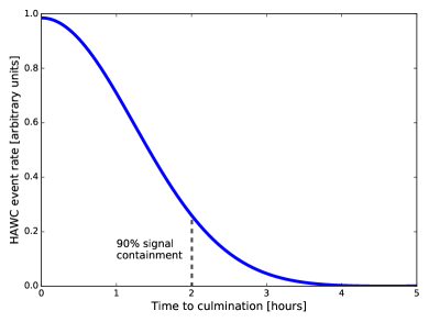
HAWC can record extensive air showers from all directions visible above the horizon. Due to the increasing absorption of secondary particles in the atmosphere, the actual effective area for gamma rays is a function of the zenith angle of the primary particle and the contribution of events from outside a cone with an opening angle of $\sim 45$ ^∘ around zenith is usually small. The field of view thus spans a solid angle of $\sim 2$ steradians (sr) and HAWC is most sensitive to sources between declinations $-26$ ^∘ and $+64$ ^∘ . With the rotation of the Earth, any location in this declination range passes over HAWC once every sidereal day. In the following, a transit is defined by visibility over HAWC at zenith angles $\theta<45$ ^∘ and lasts approximately 6 hours for the sources discussed in this paper. The detection efficiency is not uniform during the transit and Fig. 1 shows the expected fraction of signal as a function of time relative to culmination. Approximately 90% of the signal events arrive within the central $\sim 4$ hours of a transit for a source modeled on the Crab Nebula (photon index $\Gamma=2.63$ and declination 22^∘ ). While the shape of this event distribution as a function of transit time can in principle change for different spectra and declinations, it is not significantly altered for the sources discussed in this paper, which culminate within $\leq 20$ ^∘ of zenith. For the flux measurement over a full transit, the zenith dependence of HAWC’s sensitivity simplifies to a dependence on the source’s declination that determines the expected excess and energy distribution.

Refer to caption — Figure 1: Gamma-ray signal rate in HAWC versus time, showing one half of a symmetric transit before/after culmination at 0 hours. This distribution is based on simulations for a point source at declination 20^∘ with a Crab-like simple power-law spectrum, photon index $\Gamma=2.63$ , and highlights the time window during which 90% of the events are expected.

In order to process the data in units that do not contain more than one full transit for any source, all reconstructed events are sorted into sidereal days, starting at midnight local sidereal time at the HAWC site.³³3This choice leads to transits being split in two for sources with right ascension $<3$ h or $>21$ h. Such sources, though not discussed in this paper, can be analyzed with a separate set of maps binning the data with their start times offset by 12 sidereal hours. For each sidereal day and each of the nine analysis bins, a sky map of event counts is produced by populating pixels on a HEALPix grid (Gorski et al., 2005) with an average spacing of $\sim 0.06^{\circ}$ . These maps are still dominated by hadronic background events and we use direct integration (Atkins et al., 2003) to obtain a background estimate. In this procedure, a local efficiency map is created by averaging counts in a strip of pixels over two hours in right ascension around any location. We smooth this efficiency map via a spline fit to compensate for the limited statistics in higher analysis bins. The pixels near the strongest known sources and the galactic plane are excluded during the averaging in order not to bias the result by counting gamma ray events as background. Due to the limited statistics in higher analysis bins, we perform a spline fit of the local efficiency distributions during the direct integration procedure. The estimated background counts in each pixel are stored in a second map with the same grid structure.

A quality selection is applied before including data in the maps. First, monitoring of the stability of the angular distributions of reconstructed background events is used to exclude data taken during unstable conditions, for example related to maintenance. In order to control rate stability during a sidereal day, we then fit the detector rate with a function that follows tidal effects of the atmosphere and reject short periods of data that significantly deviate from this fit. To ensure a uniform detector response, sidereal days with partial coverage are not included for a given source if the lost signal fraction is expected to exceed 50%. This expected coverage fraction is calculated by integrating the signal distribution from Fig. 1 only over those sections of the transit that are included in the data, assuming a uniform flux during 6 hours. The different right ascensions of the three sources lead to slightly different exposures which are reported in Table 1. The total observation time is calculated based on 6 hours of effective HAWC observations for an uninterrupted transit and is corrected for gaps in case of partial coverage. For the period of 513 sidereal days included in this analysis, on average 92% of transits or 22% of actual time per source are covered.

Table 1: Observation time per source after quality cuts

Source	Included Transits	Time At Zenith Angles $<45$ ^∘
		[hours]
Crab	472	2700
Mrk 421	471	2665
Mrk 501	479	2750

3.2 Flux and Spectral Analysis

For this light curve analysis, the standard HAWC maximum-likelihood method (Younk et al., 2016) is applied to the sidereal day maps in order to fit photon fluxes for each transit of selected source locations. The two extragalactic sources discussed here are modeled as gamma-ray point sources with differential flux energy spectra described by a power law with normalization $F$ at 1 TeV, photon index $\Gamma$ and an optional exponential cut-off $E_{0}$ :

\frac{dN_{\mathrm{ph}}}{dE}=F\left(\frac{E}{1\mathrm{TeV}}\right)^{-\Gamma}\exp{\left(-\frac{E}{E_{0}}\right)}\quad.

(1)

In the HAWC likelihood analysis framework, this input flux is convolved with a detector response function that includes the point spread function and efficiency of triggers and cuts, depending on primary energy and incident angle. For one source transit over HAWC, the signal hypothesis contributions as a function of zenith angle are summed and yield the expected number of events $S_{b,p}$ per analysis bin $b$ (ranging from 1 to 9) and pixel $p$ (for all pixels within a radius of 3^∘ around the source).

In cases where the coverage of a source transit is interrupted, for example due to detector down time, the lost signal fraction compared to a full transit is calculated by excluding the gap period from the integration over zenith angles (see Fig. 1) and the expected event count is reduced accordingly. For the source hypothesis defined by $\{F,\Gamma,E_{0}\}$ and the observation $\mathbf{N}$ of numbers of events in all bins and pixels, we express the likelihood as

\mathcal{L}_{S}\left(\mathbf{N},\{F,\Gamma,E_{0}\}\right)=\prod_{b}{\prod_{p}{P(N_{b,p},\lambda_{b,p})}}\quad,

(2)

where $P(N_{b,p},\lambda_{b,p})$ is the Poisson distribution for a mean expectation $\lambda_{b,p}=S_{b,p}+B_{b,p}$ , the sum of the expected signal ( $S$ ) and the number of background ( $B$ ) events estimated from data for analysis bin $b$ and pixel $p$ . In the likelihood ratio test, the result of equation (2) is compared to the likelihood value $\mathcal{L}_{B}$ for a background-only assumption ( $S_{b,p}=0$ ). We express this ratio as the difference of the logarithms of the two likelihood values and define the standard test statistic as

\mathrm{TS}=2\Delta\ln{\mathcal{L}}=2\left(\ln(\mathcal{L}_{S})-\ln(\mathcal{L}_{B})\right)\quad.

(3)

TS is then numerically maximized by iteratively changing the input parameters, yielding those values that have the highest likelihood of describing the observed data for the point source model assumption.

For the analysis in this paper, the normalization $F$ , the spectral index $\Gamma$ , and the cut-off value $E_{0}$ in equation (1) were allowed to vary when fitting the spectral shape with the time-integrated data of the whole period. For the light curve measurements, the spectral parameters $\Gamma$ and $E_{0}$ were kept constant and only the normalization $F$ was left free to vary in the likelihood maximization, since the counts during a single transit are often not sufficient for a multi-parameter fit to converge.

In the light curves shown in the results section we include all flux measurements and their uncertainties (1 standard deviation), even if they do not constitute a significant detection by themselves. The likelihood-maximization procedure can produce negative flux normalizations. These are obviously non-physical as gamma-ray flux measurements but occur when low statistics lead to an underfluctuation of the event count compared to the background estimate in a sufficient number of analysis bins.

3.3 Variability Analysis

3.3.1 Likelihood Variability Test

The maximum-likelihood approach is also used to test if the daily flux measurements in a light curve are consistent with a source flux that is constant in time over the whole period under consideration. We consider the likelihood $\mathcal{L}_{i}(M)$ for the observation in time interval $i$ under two different assumptions for the hypothesis $M$ :

•

$\mathcal{L}_{i}(F_{i})$ , where $F_{i}$ is the best-fit flux value for time interval $i$ , as obtained from a likelihood maximization with only this flux as a free parameter. The light curves show these flux values $F_{i}$ .
•

$\mathcal{L}_{i}(F_{\mathrm{const}})$ , where $F_{\mathrm{const}}$ is the best-fit flux value for the time-integrated data set, as obtained from a likelihood maximization with only this flux as a free parameter.

These definitions allow us to compare the likelihood of individual flux measurements with that of a constant flux. Similar to Section 3.6 of Nolan et al. (2012), we define a test statistic as twice the differences between the logarithms of these likelihood values, summed over all intervals:

\mathrm{TS}_{\mathrm{var}}=2\sum_{i}{\left(\ln{\mathcal{L}_{i}(F_{i})}-\ln{\mathcal{L}_{i}(F_{\mathrm{const}})}\right)}\quad.

(4)

If the null hypothesis of a constant flux is true, then the distribution of TS_var can be approximated as $\chi^{2}(n_{\mathrm{dof}}-1)$ , according to Wilks’ theorem (Wilks, 1938). By applying this variability test to light curves of empty sky locations, we found that $\chi^{2}(n-1)$ indeed matches the distribution of TS_var for random fluctuations around zero if we use an effective $n=1.06n_{\mathrm{dof}}$ , where $n_{\mathrm{dof}}$ is the number of degrees of freedom in the light curve. We calculate the probability for a given source to be consistent with the constant flux hypothesis by integrating the $\chi^{2}(n-1)$ distribution above the TS_var value obtained for the light curve of that source.

3.3.2 Bayesian Blocks

If a light curve is variable, we can use the Bayesian blocks algorithm (Scargle et al., 2013) to find an optimal segmentation of the data into regions that are well represented by a constant flux, within the statistical uncertainties. We adopted the so-called point measurements fitness function for the Bayesian blocks algorithm, described in Section 3.3 of Scargle et al. (2013) and applied it to the daily flux data points to find the change points at the transition from one flux state to the next. The algorithm requires the initial choice of a Bayesian prior, called $\mathrm{ncp}_{\mathrm{prior}}$ , for the probability of finding a new change of flux states, where $\gamma=\exp{(-\mathrm{ncp}_{\mathrm{prior}})}$ is the constant factor defining a priori how much less likely it is to find $k+1$ change points instead of $k$ points. In order to choose this prior, we simulated light curves for random fluctuations around a constant flux value and required a false positive probability of 5% for finding one change point. We found this to be fulfilled by adopting $\mathrm{ncp}_{\mathrm{prior}}=6$ . We checked that varying the number of light curve points between 400 and 500 as well as using different relative uncertainties in the simulation to cover the range of observations for our three sources has negligible effect on the derived $\mathrm{ncp}_{\mathrm{prior}}$ value. The false positive probability accounts for any internal trials of the algorithm and results in a relative frequency of 5% for identifying a change point that is not a true flux state change for each light curve (see Section 2.7 of Scargle et al., 2013). The values of the constant flux amplitude within each block, defined by the position of the change points, are the averages of the corresponding daily measurements, weighted by the inverse square of the individual flux uncertainties.

3.4 Multiwavelength Correlations

A detailed comparison of simultaneous multiwavelength data for features observed in the HAWC light curves is beyond the scope of this paper. Instead, we present a first look at multi-instrument comparisons of unbiased, long-term monitoring that, like the HAWC data, provide daily binning and are not affected by seasonal visibility or weather-related gaps. Public data with comparable sampling and duty cycle for observations of Mrk 421 and Mrk 501, in particular no gaps larger than a few days, are currently only available from very few other monitoring instruments. We checked the lower energy gamma-ray light curves with daily binning from the Fermi Large Area Telescope (LAT) Monitored Source List⁴⁴4The Fermi-LAT Monitored Source List Light Curves can be found at http://fermi.gsfc.nasa.gov/ssc/data/access/lat/msl_lc., with an energy coverage from 100 MeV to 300 GeV. For neither Mrk 421 nor Mrk 501 strong flares were detected on a 1-day timescale and none of the daily-averaged integral fluxes exceeded a typical Fermi-LAT alert threshold of $10^{-6}$ ph cm^-2 s^-1 . These results were generated by an automated analysis pipeline and a re not suitable for detailed comparisons of absolute fluxes. A dedicated analysis and the study of the correlation between the high energy emission detected by Fermi-LAT and the HAWC TeV data will be presented in a forthcoming publication.

In the X-ray band, we can compare our data to the daily light curves provided by the Swift/Burst Alert Telescope (BAT) (Krimm et al., 2013). This instrument covers energies between 15 and 50 keV and, for catalog sources like those discussed here, has a median exposure of 1.7 hours per day that can vary throughout the year but stays $<5.4$ hours for 95% of the days. The Swift-BAT light curves are sampled with one data point per day, based on Modified Julian Dates (MJD), and are thus not perfectly aligned with the binning in local sidereal days that was chosen as a natural frequency for the HAWC data. The observations are also not necessarily exactly simultaneous on the scale of hours.

3.5 Systematic Uncertainties

A detailed analysis of systematic uncertainties of gamma-ray fluxes measured with HAWC in Abeysekara et al. (2017b) concludes with estimating a $\pm 50$ % uncertainty in the flux normalization. This uncertainty affects all per-transit flux measurements only as a common change in absolute scaling and thus does not impact the relative magnitude of daily flux measurements. The results of variability studies and change point identification can only be affected by systematic uncertainties that change between individual sidereal days or time periods. The calibration is monitored and is very stable. Updates of calibration parameters were only performed to accommodate hardware changes, for example additions of PMTs. The remaining hardware-related potential source of variability is removal or replacement of individual PMTs due to maintenance and repairs. This has been found to affect flux measurements by less than $\pm 5$ %. A higher level systematic uncertainty that could in principle affect individual fluxes is due to the possibility that the blazar spectra vary with time or flux state (see e.g. Krennrich et al., 2002). We simulated gamma-ray fluxes with different spectral parameters that are allowed within the uncertainties of our data and analyzed them with the fixed parameters used in the light curve analysis. For each source we determined an optimal threshold above which we perform the analytical flux integration by requiring that the difference between the photon fluxes for different spectral hypotheses is minimal. These threshold values are used when quoting the photon fluxes in the results sections: 1 TeV for the Crab Nebula, 2 TeV for Mrk 421, and 3 TeV for Mrk 501. The resulting uncertainty on individual flux values under spectral hardening or softening is $\pm 5$ %. The combination of these two potentially time-dependent systematic uncertainties is significantly smaller than the statistical uncertainty of the per-transit flux values and thus marginal with respect to the analysis of variability features.

We have performed further tests of the robustness of the likelihood variability estimation. Using the Crab Nebula as a reference, we found that changes in the analysis procedure with respect to background estimation (different smoothing procedures within the direct integration), data selection (excluding the three highest bins with an average $\leq 1$ photon per day for our sources), and spectral model (power law and log parabola) only changed the resulting TS_var value of the variability by $\leq 0.2$ standard deviations of the null hypothesis. We therefore find no indication that the map-making and likelihood analysis can introduce significant variability features. We conclude that our analysis of flux variations and identification of flaring states in this paper is not limited by these systematic uncertainties.

For the interpretation of absolute flux values it is helpful to compare our measurements to a gamma-ray reference flux. We therefore convert fluxes to multiples of the HAWC-measured Crab Nebula flux ( $1.89\cdot 10^{-11}$ ph cm ^-2 s^-1, see detailed analysis in Abeysekara et al., 2017b) as Crab Units (CU) with a common threshold of 1 TeV. This threshold was chosen to provide easier comparisons between the different sources and the literature. We still have to consider the flux uncertainty introduced by the choice of a fixed spectral assumption for which the analytical integration above 1 TeV is performed. We used the time-integrated HAWC data to fit the flux normalization of each of the three sources discussed here with a number of different power law indices and cut-off values that cover the individual statistical and systematic uncertainty range. We find that the maximum uncertainty of the photon fluxes in CU due to the spectral assumption is $\pm 25$ %.

4 Results for the Crab Nebula

4.1 Flux Light Curve

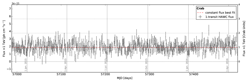
The Crab Nebula is the brightest galactic TeV point source. A detailed analysis of time-integrated HAWC data for this source is presented in Abeysekara et al. (2017b). In Fig. 2 we show the results of applying the likelihood analysis to the sidereal day maps at the location of the Crab Nebula. We use a fixed spectrum with index $\Gamma=2.63$ in equation (1) and no exponential cut-off, $E_{0}\rightarrow\infty$ , based on the best fit value obtained in the HAWC catalog (Abeysekara et al., 2017a).

The left-hand y-axis in Fig. 2 indicates the photon flux ( ph cm^-2 s^-1 ) after analytically integrating the spectrum above 1 TeV for the best fit normalization. The right-hand axis shows the Crab Units (CU) defined by dividing the flux by the time-averaged HAWC measurement of the Crab flux, also indicated as a dashed line in the figure. We use Modified Julian Dates (MJD) for labeling the time axes and highlight the duration of HAWC measurements (6 sidereal hours) through horizontal bars.

We applied the variability test outlined in Section 3.3 to the light curve with 1-transit intervals and found a $\mathrm{TS}_{\mathrm{var}}=517.9$ , with a probability of 0.292 ( $1.1$ standard deviations) of measuring the same or a larger TS value for a constant flux hypothesis. An analysis of the light curve with the Bayesian blocks algorithm with a false positive probability of 5% reveals no change points. HAWC daily flux measurements thus show no indication of variability in data from the Crab Nebula.

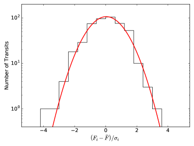
In Fig. 3 we show a histogram of $(F_{i}-\bar{F})/\sigma_{i}$ , where $F_{i}$ and $\sigma_{i}$ are the fluxes and uncertainties from Fig. 2 and $\bar{F}$ is the best fit value for a constant flux. A fit to a Gaussian function yields a center at $0.035\pm 0.050$ and a width of $1.033\pm 0.036$ , confirming that the observed flux distribution is consistent with arising from a constant source flux.

4.2 Discussion

Based on measurements by other instruments, the Crab is generally believed to be a steady source⁵⁵5We ignore here the very high energy pulsed emission directly from the pulsar that is very weak compared to the pulsar wind nebula’s emission. at TeV energies (Aliu et al., 2014; Abramowski et al., 2014; Bartoli et al., 2015). The non-detection of variability in TeV emission from the Crab Nebula with HAWC is in agreement with these results. We conclude that HAWC daily light curve measurements and the likelihood variability check are a robust test of the steady gamma-ray source hypothesis and that any systematic uncertainties in the HAWC data are very unlikely to mimic significant variability in this analysis.

Given that the Crab Nebula is known to flare in lower energy bands, we can use the unique daily TeV light curve data to constrain any TeV flux enhancement during such episodes. During the 17 months included here, the Fermi-LAT collaboration reported an increased gamma-ray flux for energies $>100$ MeV between 2015 December 28 and 2016 January 9, reaching up to $\sim 1.7$ times the average flux (Buehler et al., 2016). The maximum HAWC 1-transit flux during this period was $(2.14\pm 0.54)\cdot 10^{-11}$ ph cm^-2 s^-1 above 1 TeV on 2016 January 7, only 0.46 standard deviations above the average flux. This corresponds to an upper limit at 95% confidence level of $3.04\cdot 10^{-11}$ ph cm^-2 s^-1 above 1 TeV, 1.6 times the average flux. When we combine the HAWC measurements over the 12 transits⁶⁶6Two out of 14 transits did not pass the quality criterion of $>50$ % transits coverage. included in this period, we obtain a flux measurement of $(1.42\pm 0.15)\cdot 10^{-11}$ ph cm^-2 s^-1 above 1 TeV, 0.75 times the average flux and consistent with a random fluctuation. We conclude that we observe no significant change in the TeV flux during this MeV flare period.

5 Results for Mrk 421

5.1 Source Characteristics

Mrk 421 is a BL Lacertae type blazar with a redshift of $z=0.031$ (Mao, 2011). It was the first extragalactic object discovered in the TeV band (Punch et al., 1992) and has been extensively studied by many TeV gamma-ray observatories. Mrk 421 is known to exhibit a high degree of variability in its emission and yearly average fluxes are known to vary between a few tenths and $\sim 1.9$ times the flux of the Crab Nebula (Acciari et al., 2014). Variability has been observed down to time scales of hours or less and its spectral shape is known to vary with its brightness (Krennrich et al., 2002).

By using the time-integrated HAWC data for Markarian 421, we fit the spectral shape with the likelihood methods discussed in Section 3.2, leaving the normalization $F$ , the photon index $\Gamma$ , and the exponential cut-off $E_{0}$ free. The resulting best fit values are $F=(2.82\pm 0.19_{\mathrm{stat}}\pm 1.41_{\mathrm{sys}})\cdot 10^{-11}$ TeV^-1 cm^-2 s^-1 for the time-averaged normalization at 1 TeV, a photon index $\Gamma=2.21\pm 0.14_{\mathrm{stat}}\pm 0.20_{\mathrm{sys}}$ and an exponential cut-off at $E_{0}=5.4\pm 1.1_{\mathrm{stat}}\pm 1.0_{\mathrm{sys}}$ TeV. The significance of this description over the background-only hypothesis is $\mathrm{TS}=1232.47$ or 35.1 standard deviations. When compared to a pure power law hypothesis ( $E_{0}\rightarrow\infty$ ), the fit with a cut-off is clearly the better description, preferred at $\Delta\mathrm{TS}=64.8$ or 8 standard deviations. We use these values for index and cut-off as a fixed set of parameters when fitting the flux normalization for each sidereal day, reported in the following section.

5.2 Flux Light Curve

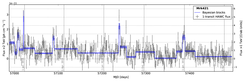
The flux light curve for Mrk 421 with 1-transit intervals is shown in Fig. 4 . Photon flux units (left y-axis) are based on analytical integration of the fixed spectral shape above a threshold of 2 TeV that minimizes flux uncertainties due to spectral variations. The conversion to CU (right axis) is based on average HAWC Crab Nebula measurements, see Section 4, for a common threshold of 1 TeV in order to allow comparisons between the different sources. The average flux for the 17 months period is determined via a fit of the combined data under a constant flux assumption and yields $(4.53\pm 0.14)\cdot 10^{-12}$ ph cm^-2 s^-1 above 2 TeV.

Applying the likelihood variability test to this light curve yields TS ${}_{\mathrm{var}}=1154.9$ , which corresponds to a p-value $4.40\cdot 10^{-54}$ based on the expected $\chi^{2}$ distribution for constant flux models and clearly shows the variable nature of the TeV emission from Mrk 421. The highest per-transit flux value, $(2.94\pm 0.37)\cdot 10^{-11}$ ph cm ^-2 s^-1 above 2 TeV was measured for MJD 57238.74 – 57238.99 (2015-08-04 UTC 17:40 – 23:40), with a pre-trial significance of 9.3 standard deviations compared to the null hypothesis. A flux that is only slightly lower, $(2.91\pm 0.38)\cdot 10^{-11}$ ph cm ^-2 s^-1, was observed during MJD 57020.33 – 57020.58 (2014-12-29 UTC 8:00 – 14:00) and highlights that the variability occurs on time scales of less than one day, since the flux value for the day before and after this maximum are a factor of $\sim 3$ and $\sim 4$ lower, respectively.

The Bayesian blocks algorithm with a prior corresponding to a false positive probability of 5% identifies 18 change points in the light curve shown in Fig. 4. The flux amplitudes for the periods between two change points that are consistent with a constant flux are included as blue lines with a shaded region for the statistical uncertainty of one standard deviation. These block positions and amplitudes are listed in Table 2 in the Appendix.

5.3 Discussion

The spectral fit results, $\Gamma=2.21\pm 0.14_{\mathrm{stat}}\pm 0.20_{\mathrm{sys}}$ and $E_{0}=5.4\pm 1.1_{\mathrm{stat}}\pm 1.0_{\mathrm{sys}}$ TeV, are consistent with spectral shapes previously observed (see e.g. Albert et al., 2007b). If we compare to the range of VERITAS spectral fits as a function of flux state in Acciari et al. (2011a), we find that the average HAWC spectrum is closest to the parameters for the Mid-state level, $\Gamma^{\mathrm{M}}=2.278\pm 0.037$ and $E_{0}^{\mathrm{M}}=4.36\pm 0.58$ TeV. A more detailed analysis of the HAWC spectral fits and a discussion of the absorption features of the EBL is beyond the scope of this paper. We will revisit this in a separate paper and take advantage of better energy estimation techniques for HAWC data that are currently under development to enhance the sensitivity to the curvature at the highest energies.

HAWC data can confirm and track the variability of Mrk 421 via daily flux measurements. By applying the Bayesian blocks algorithm, we identified 19 distinct flux states. The apparent substructure within some blocks in Figure 4 is likely to be due to flux variations on shorter time scales which cannot be resolved by the present analysis, given the predetermined 5% false positive probability and the uncertainties of our measurements. As a stability check, we lowered the false positive condition from 5% to 10%, which led to the identification of only one additional block around MJD 57065.

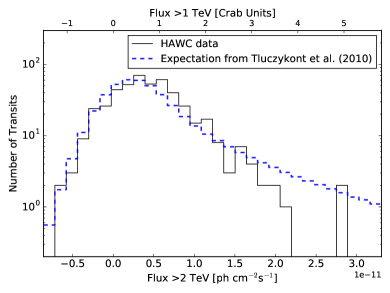
In Fig. 5, a histogram of all flux measurements from Mrk 421 highlights the spread of the observed flux states. We can compare this distribution to a function from Tluczykont et al. (2010) that was derived as a good fit to archival data, composed of the sum of a normal distribution ( $f_{\mathrm{Gauss}}$ ) around a low flux peak and a log-normal part ( $f_{\mathrm{LogN}}$ ) describing a tail to higher fluxes. The number of observations as a function of the flux $x$ is given by:

$\displaystyle f_{T}(x)$	$\displaystyle=$	$\displaystyle f_{\mathrm{Gauss}}+f_{\mathrm{LogN}}$
	$\displaystyle=$	$\displaystyle\frac{n_{\mathrm{Gauss}}}{\sigma_{\mathrm{Gauss}}\sqrt{2\pi}}\exp{\left(-\frac{(x-\mu_{\mathrm{Gauss}})^{2}}{2\sigma_{\mathrm{Gauss}}^{2}}\right)}$
		$\displaystyle+\frac{n_{\mathrm{LogN}}}{x\sigma_{\mathrm{LogN}}\sqrt{2\pi}}\exp{\left(-\frac{(\ln(x)-\mu_{\mathrm{LogN}})^{2}}{2\sigma_{\mathrm{LogN}}^{2}}\right)}\;,$

with the best-fit parameters $n_{\mathrm{Gauss}}=48.08$ , $\mu_{\mathrm{Gauss}}=0.3285$ , $\sigma_{\mathrm{Gauss}}=0.1137$ , $n_{\mathrm{LogN}}=45.55$ , $\mu_{\mathrm{LogN}}=0.1025$ , and $\sigma_{\mathrm{LogN}}=1.022$ . Here we follow the convention from the reference of measuring $x$ in CU above 1 TeV but setting its unit to 1 in the formula. In order to account for the HAWC measurement uncertainties, we use a two-step process to define samples that each have 471 flux values, matching the size of the data set. First, we draw 471 random values according to the distribution in equation (5.3) and use these value as centers and the standard deviation values from data as widths to define 471 normal distributions. Then, we draw one random value form each of these normal distributions to obtain a set of fluxes that reflects the uncertainties of the HAWC data. We average over 10,000 such samples to obtain the prediction for a HAWC measurement of this flux distribution. It is included in Fig. 5 (blue, dashed line). We compare this expectation with the histogram of HAWC data via a Kolmogorov-Smirnov (KS) test and find a probability of $0.0008$ that they arise from the same distribution. This value is stable under changes of the histogram binning and rescaling the HAWC fluxes within the systematic uncertainty of $\pm 25$ % leads to a maximum KS probability value of $0.0046$ . Since we account for HAWC flux uncertainties in our sampling procedure, we also tested reducing $\sigma_{\mathrm{Gauss}}$ from Tluczykont et al. (2010) under the assumption that it is mostly reflecting measurement uncertainties in the fitted data, but found only smaller KS probabilities. Since equation (5.3) is based on the fit to a compilation of measurements from many different instruments, it is hard to assess the systematic uncertainties of this parametrization. We have to consider that the large gaps in time coverage and a likely bias due to observations triggered by multiwavelength alerts for the public data in Tluczykont et al. (2010) can lead to a fit that does not well represent the average daily flux distribution for Mrk 421. We compare this function here for the first time with data from an unbiased, regular monitoring with a single, stable detector and conclude that these 17 months of HAWC observations cannot be well described by equation (5.3). The current level of statistical uncertainties of the HAWC data prevents us from obtaining a stable fit of the 6 parameters from equation (5.3) or testing if the tail of higher fluxes is indeed best described with a log-normal distribution which could indicate an origin of variability from multiplicative processes. Increased statistics and the coverage of more high flux states with new HAWC data will provide the basis for obtaining a better functional description of Mrk 421 flux states.

Since February 2016, the daily flux measurements for both Mrk 421 and Mrk 501 have been automatically performed at the HAWC site immediately after the end of each transit. The preliminary analysis is based on the so-called online reconstruction, performed with only a few seconds’ time lag on all recorded events and a preliminary calibration and data quality selection. Our threshold for issuing alerts about flaring states for both sources is a flux value equivalent to 3 CU in a single transit, which corresponds to a detection at $\sim 5$ standard deviations for Mrk 421. In the 17 months of data included here, Mrk 421 surpassed this threshold during 11 transits, 2.3% of the time.

5.4 Multiwavelength Comparisons

In Fig. 6, we compare the HAWC TeV measurements to light curves from the Swift-BAT (15 – 50 keV)⁷⁷7Public light curve data from http://swift.gsfc.nasa.gov/results/transients/. monitoring instrument that provides very similar sampling and instrument duty cycle. The Swift-BAT data allow us to apply the same Bayesian blocks algorithm as used for HAWC data. The ratio of average error to mean flux value is larger for Swift-BAT light curves than for the HAWC data, but simulations show that the same Bayesian prior value ( $\mathrm{ncp}_{\mathrm{prior}}=6$ ) will guarantee the same false positive probability of 5%. This analysis identifies 8 change points, i.e. 9 blocks, in the X-ray data. The only Swift-BAT flux state that matches one of the HAWC flux states with less than 10 days’ difference in start and end times is the lowest one ⁸⁸8The Swift-BAT weighted mean amplitude for this block is negative but compatible with zero within 1.1 standard deviations.. None of the highest HAWC-measured flaring states are mirrored in the blocks for the X-ray light curve. We cannot exclude that the size of the statistical uncertainties hides correlated features at the day scale, considering that at least the Swift-BAT energy band seems to cover mostly a steeply falling part of the spectral energy distribution observed in the past (Abdo et al., 2011b). It is possible that this is due to insufficient overlap between the instruments’ exposures during one day, since we established significant TeV variability within less than one sidereal day in Section 5.2. Similar cases of missing correlations for bright TeV flares have been observed before (see e.g. Acciari et al., 2011a; Blazejowski et al., 2005). On the other hand, when we compare all daily averaged fluxes by calculating the Spearman rank correlation coefficient for the HAWC and the Swift-BAT data we find a positive correlation of $0.341\pm 0.030$ . The probability for this result to occur for uncorrelated data sets of the same size is $3\cdot 10^{-13}$ and we can thus qualitatively confirm previous observations of TeV-to-keV correlations based on (partially biased) IACT data (Fossati et al., 2008; Blazejowski et al., 2005; Albert et al., 2007b; Horan et al., 2009; Tluczykont et al., 2010) .

The only public notification about flaring activity for Mrk 421 that was sent during the period under investigation is an Astronomer’s Telegram (Kapanadze, 2015) about an increased X-ray flux observed with Swift-XRT (0.3 – 10 keV) between June 8 and June 16, 2015. Our Bayesian blocks analysis does not identify any significant flux state changes within 1.2 months around these dates.

6 Results for Mrk 501

6.1 Source Characteristics

Mrk 501 is a BL Lacertae type blazar that is similar to Mrk 421, given its distance of $z=0.033$ (Mao, 2011) and its classification as a high-peaked BL Lac object. It is the second extragalactic object that was discovered at TeV energies (Quinn et al., 1996). Various studies at TeV energies have shown different features of low flux states emission and extreme outbursts, for example in Acciari et al. (2011b).

Our initial fit of the spectral shape uses the integrated 17 months of HAWC data. When we do not allow curvature in the spectral model, $E_{0}\rightarrow\infty$ in equation 1, we obtain the best fit values $F=(4.50\pm 0.28_{\mathrm{stat}}\pm 2.25_{\mathrm{sys}})\cdot 10^{-12}$ TeV^-1 cm^-2 s^-1 for normalization at 1 TeV and a photon index $\Gamma=2.84\pm 0.04_{stat}\pm 0.20_{sys}$ . This is consistent with results reported in Acciari et al. (2011b) and Abdo et al. (2011a). Leaving also the exponential cut-off free yields a normalization $F=(4.40\pm 0.60_{\mathrm{stat}}\pm 2.20_{\mathrm{sys}})\cdot 10^{-12}$ TeV^-1 cm^-2 s^-1 , a photon index $\Gamma=1.60\pm 0.30_{\mathrm{stat}}\pm 0.20_{\mathrm{sys}}$ , and an exponential cut-off value of $E_{0}=5.7\pm 1.6_{\mathrm{stat}}\pm 1.0_{\mathrm{sys}}$ TeV. The latter result is clearly preferred by $\Delta\mathrm{TS}=48.64$ or 7.0 standard deviations over the power law fit without a cut-off. Its significance compared to the background-only hypothesis is $\mathrm{TS}=610.49$ or 24.7 standard deviations. For the flux normalization fits performed to construct the flux light curve we use the description with the cut-off and keep the index and cut-off parameters fixed at the HAWC-measured values.

6.2 Flux Light Curve

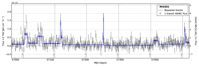
The Mrk 501 flux light curve for all 1-transit intervals that have $>50$ % coverage with HAWC is shown in Fig. 7. The photon flux is calculated as the analytical integration above 3 TeV, the optimal threshold value for Mrk 501 in order to minimize the systematic uncertainties of the flux measurement due to the fixed spectral assumption. For the 17 months period included here, we find an average flux of $(1.74\pm 0.08)\cdot 10^{-12}$ ph cm^-2 s^-1 above 3 TeV.

The result of the likelihood variability calculation for Mrk 501 is TS ${}_{\mathrm{var}}=1115.4$ , corresponding to a p-value $9.18\cdot 10^{-48}$ , and thus clearly establishes variability of the TeV emission measured here. The highest daily flux, $(1.67\pm 0.23)\cdot 10^{-11}$ ph cm^-2 s^-1 above 3 TeV, was observed during the transit MJD 57251.94 – 57252.19 (2015-08-17 UTC 22:40 to 2015-08-18 UTC 4:40) with a pre-trial significance of 9.5 standard deviations compared to the null hypothesis. This is approximately a factor 10 higher than the constant flux fit average and shows a variability time scale of less than one day, since the flux is higher by a factor $\sim 4$ compared to the previous transit and by a factor $\sim 8$ compared to the next transit.

In order to find significant flux state changes in this light curve, we applied the Bayesian blocks algorithm. Given the prior for 5% false positive probability, the algorithm identifies 13 change points. The amplitudes of periods between these change points are consistent with a constant flux and are shown as blue lines in Fig. 7, with shaded bands indicating one standard deviation around the mean amplitude. These block positions and amplitudes are listed in Table 3 in the Appendix.

6.3 Discussion

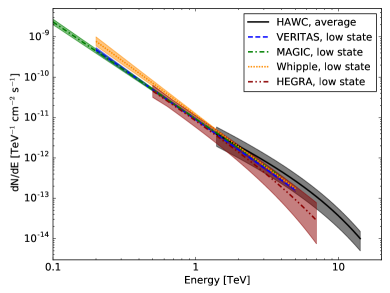
The integrated HAWC data for Mrk 501 is best described via a curved spectrum that we model with a photon index $\Gamma=1.6$ and an exponential cut-off at $E_{0}=5.7$ TeV. In Fig. 8 we compare this result with spectra measured by MAGIC (Ahnen et al., 2016), VERITAS and Whipple (Aliu et al., 2016), as well as HEGRA (Aharonian et al., 2001). We include only the values designated as low-state by these observatories since the HAWC light curve shows long periods of low activity that dominate our averaged measurement. The analyses of spectra during flaring states in the same publications show generally harder photon indices. The HAWC spectrum averaged over 17 months is consistent with these measurements within the statistical and systematic uncertainties as shown in Fig. 8. The spectral curvature in our measurement manifests itself primarily outside the energy range covered by the IACT measurements. The HAWC energy range was determined from simulation as the central interval containing 90% of expected signal events for the best-fit spectrum. While the strong curvature in the spectrum of Mrk 501 prevents us from constraining the spectral shape above an energy of $\sim$ 15 TeV with the current analysis, HAWC is generally sensitive to gamma ray energies up to $\sim$ 100 TeV, as discussed in Abeysekara et al. (2017a).

The HEGRA analysis also obtains a better fit with an exponential cut-off than a pure power law. The HEGRA cut-off value, $5.1(_{-2.3}^{+7.8})_{\mathrm{stat}}$ TeV, is consistent with the HAWC value. A cut-off in the energy spectrum can arise from gamma-ray absorption through the EBL (see e.g. Domínguez et al., 2011) or originate in processes intrinsic to the source, for example, a limit to the energies of injected particles, changes in the Klein-Nishina scattering cross section (Hillas, 1999), or absorption through photon fields in the lower jet (Dermer & Schlickeiser, 1994). The best-fit photon index $\Gamma=1.6\pm 0.30_{\mathrm{stat}}\pm 0.20_{\mathrm{stat}}$ that we measure is hard compared to, for example, Mrk 421 but still greater than the lower limit of $\sim 1.5$ for Fermi-acceleration in shocks (Malkov & Drury, 2001). At lower energies, up to $\sim~{}300$ GeV, spectral hardening with photon indices down to $\sim 1.0$ has been observed for Mrk 501 by Fermi-LAT (see e.g. Shukla et al., 2016). We will provide a more detailed study of the spectral energy distribution and EBL absorption for Mrk 501 with HAWC data in a separate publication.

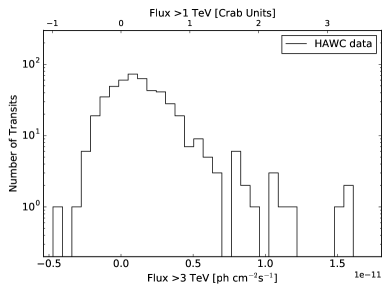
The TeV light curve for Mrk 501 shows various flaring periods and we find 14 Bayesian blocks defining distinct flux states under a false detection prior of 5%. The three highest per-transit fluxes exceed the level of three times the Crab Nebula flux, corresponding to 0.6% of all observations included here. The last of these flares (2015 August 17) was also captured in tests of the HAWC real-time fast transient monitor (Weisgarber, 2017) that resolves a sub-transit light curve of event rates. A histogram of all flux measurements is shown in Fig. 9. The shape is generally similar to Fig. 5, though with the peak and maximum fluxes shifted to lower CU values. As in the case of Mrk 421, the limited statistics currently prevent us from distinguishing between different functional descriptions of this distribution.

The automated daily light curve monitor that performs the per-transit light curve analysis at the HAWC site has been operational since 2016 February and identified the increased flux state of Mrk 501 on 2016 April 6, is visible on the right side of Fig. 7 at a level of $\sim 2.4$ CU. We reported this flare in Sandoval et al. (2016), including the fact that the following day still showed a higher than average flux before returning to a lower state. The gamma-ray excess rates measured by FACT⁹⁹9See public monitoring at http://www.factproject.org/monitoring (Anderhub et al., 2013). above 750 GeV also show a rising trend before the HAWC alert.

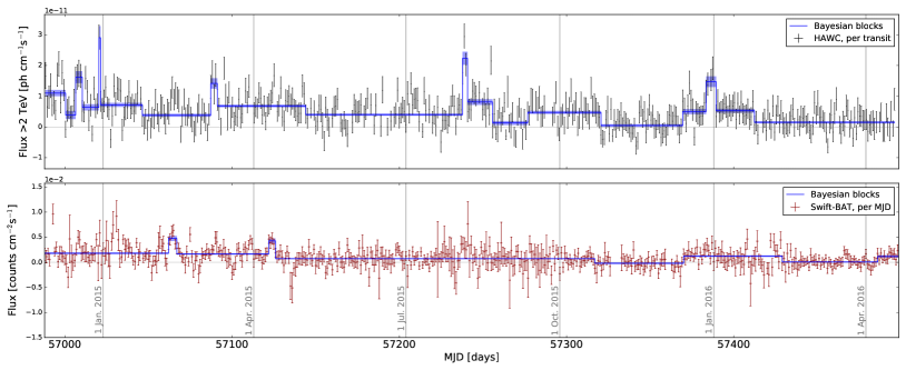
6.4 Multiwavelength Comparisons

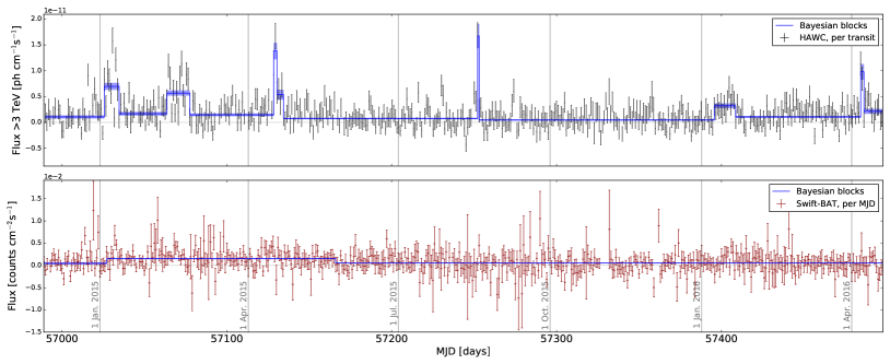
The Swift-BAT (15 – 50 keV) data¹⁰¹⁰10Public light curve data from http://swift.gsfc.nasa.gov/results/transients/. for Mrk 501 have a very high ratio of average error to weighted mean flux (2.5), but we can apply the same Bayesian blocks analysis with prior value $\mathrm{ncp}_{\mathrm{prior}}=6$ as for HAWC data, keeping a 5% false positive probability. Only 2 change points, i.e. 3 distinct flux states are found. The resulting comparison between the three light curves is shown in Fig. 10. The X-ray data reveal no day-scale light curve features that are correlated with the TeV flares observed with HAWC. With the Bayesian blocks analysis we find no short flaring periods in the Swift-BAT light curves that mirror the activity observed at TeV energies, but the large relative uncertainties (average error corresponds to 2.5 times the mean rate value) precludes us from obtaining a quantitative limit for this absence of correlation. We can calculate the Spearman rank correlation coefficient for all daily averaged fluxes and obtain $0.164\pm 0.032$ , with a probability of $10^{-3}$ to occur for an uncorrelated system. This positive correlation is qualitatively similar to results obtained previously (e.g. Krawczynski et al., 2000; Tluczykont et al., 2010) but is less significant than that observed for Mrk 421 in Section 5.4.

7 Conclusions and Outlook

We presented the first TeV gamma-ray light curves with sidereal day binning for the Crab Nebula, Markarian 421, and Markarian 501 that were obtained with the first 17 months of data from the HAWC Observatory. HAWC is currently the most sensitive wide-field-of-view TeV gamma-ray observatory and provides unique coverage of transients due to its $\sim 95$ % duty-cycle and an unbiased daily observation mode.

No variability was found for the Crab Nebula flux measurements, which is in agreement with the absence of TeV variability in IACT observations. For both Mrk 421 and Mrk 501 we found clear variability on time scales of one day and use the Bayesian blocks algorithm to identify distinct flux states. In the case of Mrk 421, the distribution of unbiased, daily flux measurements from HAWC is not well described by a fit to archival TeV data from literature. The average flux over the period included here is $\sim 0.8$ CU above 1 TeV, significantly higher than previous estimates for an upper limit to the baseline flux ( $\sim 0.3$ CU) but not exceeding the maximum of past yearly averages. The highest flux values, averaged over 6 hours, reach up to five times the Crab Nebula flux. Mrk 501, on the other hand, is observed with an average flux $\sim 0.3$ CU above 1 TeV, with flares reaching up to $\sim 3.5$ CU multiple times during our observations. The spectral fit for Mrk 501 is in agreement with previous measurements up to a few TeV and shows curvature, modeled here as an exponential cut-off at $\sim 6$ TeV.

The public monitoring data for lower energy gamma rays with Fermi-LAT (100 MeV to 300 GeV) did not show daily flaring features during the period covered by our TeV light curves. We compared the HAWC data to Swift-BAT X-ray measurements that have similar sampling and duty cycle. For daily intervals, we could not identify activity in this energy band (15 to 50 keV) that is correlated with the largest TeV flaring episodes observed with HAWC. On the other hand, we find positive correlations for both Mrk 421 and Mrk 501 between HAWC and Swift-BAT X-ray fluxes when comparing all daily averaged measurements, similar to previously published results. This first look at multiwavelength correlations is limited by the low sensitivities of the satellite monitoring instruments that result in large uncertainties for average daily fluxes. In a forthcoming study, we will extend these multiwavelength studies and include data from pointed observations with more sensitive instruments where available, in order to better assess flux correlations and compare them to broad band model predictions. Ongoing work of improving the energy estimation in the HAWC analysis will help us to study the spectra of Mrk 421 and Mrk 501 in more detail and to investigate changes in spectral behavior over time.

The description of the methods, systematic uncertainties, and reference applications of the HAWC light curve analysis that we presented here provides the basis for day-scale transient studies of any TeV source within the approximately two thirds of the sky monitored by HAWC. This analysis is already being performed in realtime and will continue to provide flare alerts for Mrk 421 and Mrk 501. We are in the process of applying this analysis to all candidates listed in the HAWC catalog (Abeysekara et al., 2017a), as well as other target lists, and will present those results in a separate publication.

The HAWC Observatory will continue to record unbiased data for every source location transiting through its field of view, with an exposure of up to 6 hours per sidereal day. With the initial results discussed here and the continuation of this analysis program over the following years, we aim to provide HAWC TeV light curves as a new resource for studying the time domain of astrophysical processes at the highest energies.

8 Acknowledgements

We acknowledge the support from: the US National Science Foundation (NSF); the US Department of Energy Office of High-Energy Physics; the Laboratory Directed Research and Development (LDRD) program of Los Alamos National Laboratory; Consejo Nacional de Ciencia y Tecnología (CONACyT), México (grants 271051, 232656, 260378, 179588, 239762, 254964, 271737, 258865, 243290, 132197), Laboratorio Nacional HAWC de rayos gamma; L’OREAL Fellowship for Women in Science 2014; Red HAWC, México; DGAPA-UNAM (grants RG100414, IN111315, IN111716-3, IA102715, 109916, IA102917); VIEP-BUAP; PIFI 2012, 2013, PROFOCIE 2014, 2015;the University of Wisconsin Alumni Research Foundation; the Institute of Geophysics, Planetary Physics, and Signatures at Los Alamos National Laboratory; Polish Science Centre grant DEC-2014/13/B/ST9/945; Coordinación de la Investigación Científica de la Universidad Michoacana. Thanks to Luciano Díaz and Eduardo Murrieta for technical support.

Appendix A Bayesian Blocks results

Tables 2 and 3 show the Bayesian block results (5% false positive probability) from the analysis of HAWC daily flux light curves for Mrk 421 and Mrk 501, respectively.

Table 2: HAWC Bayesian blocks for Mrk 421

MJD Start	MJD Stop	Duration	Flux $>2$ TeV
		[days]	[ph cm^-2 s^-1]
56988.38	56999.64	12.01	$(1.1\pm 0.1)\cdot 10^{-11}$
57000.39	57005.63	5.98	$(3.9\pm 1.3)\cdot 10^{-12}$
57006.37	57009.61	3.99	$(1.6\pm 0.2)\cdot 10^{-11}$
57010.36	57019.59	9.97	$(6.4\pm 1.0)\cdot 10^{-12}$
57020.33	57020.58	1.00	$(2.9\pm 0.4)\cdot 10^{-11}$
57021.33	57045.52	24.93	$(7.2\pm 0.7)\cdot 10^{-12}$
57046.26	57086.40	40.89	$(3.8\pm 0.5)\cdot 10^{-12}$
57087.15	57090.39	3.99	$(1.4\pm 0.2)\cdot 10^{-11}$
57091.14	57143.25	52.85	$(6.9\pm 0.5)\cdot 10^{-12}$
57144.00	57236.99	93.74	$(4.0\pm 0.4)\cdot 10^{-12}$
57237.74	57239.98	2.99	$(2.2\pm 0.2)\cdot 10^{-11}$
57240.73	57254.95	14.96	$(8.1\pm 0.9)\cdot 10^{-12}$
57255.69	57275.89	20.94	$(1.3\pm 0.7)\cdot 10^{-12}$
57276.63	57319.76	43.88	$(4.7\pm 0.5)\cdot 10^{-12}$
57320.51	57368.63	48.87	$(4.8\pm 4.2)\cdot 10^{-13}$
57369.38	57382.59	13.96	$(5.0\pm 0.8)\cdot 10^{-12}$
57383.34	57387.58	5.98	$(1.5\pm 0.2)\cdot 10^{-11}$
57389.32	57411.51	22.94	$(5.3\pm 0.6)\cdot 10^{-12}$
57412.26	57496.28	83.77	$(1.5\pm 0.3)\cdot 10^{-12}$

Table 3: HAWC Bayesian blocks for Mrk 501

MJD Start	MJD Stop	Duration	Flux $>3$ TeV
		[days]	[ph cm^-2 s^-1]
56989.66	57024.82	35.90	$(1.1\pm 0.3)\cdot 10^{-12}$
57025.56	57033.79	8.98	$(7.0\pm 0.7)\cdot 10^{-12}$
57034.54	57062.67	28.92	$(1.7\pm 0.3)\cdot 10^{-12}$
57063.46	57076.67	13.96	$(5.7\pm 0.5)\cdot 10^{-12}$
57077.42	57127.53	50.86	$(1.5\pm 0.3)\cdot 10^{-12}$
57128.28	57129.53	1.99	$(1.4\pm 0.2)\cdot 10^{-11}$
57130.28	57133.52	3.99	$(5.4\pm 1.0)\cdot 10^{-12}$
57134.27	57251.20	117.68	$(7.6\pm 1.5)\cdot 10^{-13}$
57251.94	57252.19	1.00	$(1.7\pm 0.2)\cdot 10^{-11}$
57252.94	57394.80	142.61	$(4.5\pm 1.4)\cdot 10^{-13}$
57395.55	57407.77	12.96	$(3.2\pm 0.5)\cdot 10^{-12}$
57408.51	57483.56	75.79	$(1.1\pm 0.2)\cdot 10^{-12}$
57484.31	57485.55	1.99	$(9.8\pm 1.5)\cdot 10^{-12}$
57486.30	57497.52	10.97	$(2.1\pm 0.5)\cdot 10^{-12}$

References

Abdo et al. (2011a) Abdo, A. A., et al. 2011a, ApJ, 727, 129
Abdo et al. (2011b) —. 2011b, ApJ, 736, 131
Abdo et al. (2014) —. 2014, ApJ, 782, 110
Abeysekara et al. (2017a) Abeysekara, A. U., et al. 2017a, arXiv:1702.02992
Abeysekara et al. (2017b) —. 2017b, arXiv:1701.01778
Abramowski et al. (2014) Abramowski, A., et al. 2014, A&A, 562, L4
Acciari et al. (2011a) Acciari, V. A., et al. 2011a, ApJ, 738, 25
Acciari et al. (2011b) —. 2011b, ApJ, 729, 2
Acciari et al. (2014) —. 2014, Astropart. Phys., 54, 1
Aharonian et al. (2001) Aharonian, F., et al. 2001, ApJ, 546, 898
Aharonian et al. (2007) —. 2007, ApJ, 664, L71
Ahnen et al. (2016) Ahnen, M. L., et al. 2016, ArXiv e-prints, arXiv:1612.09472
Albert et al. (2007a) Albert, J., et al. 2007a, ApJ, 669, 862
Albert et al. (2007b) —. 2007b, ApJ, 663, 125
Aliu et al. (2014) Aliu, E., et al. 2014, ApJ, 781, L11
Aliu et al. (2016) —. 2016, A&A, 594, A76
Anderhub et al. (2013) Anderhub, H., et al. 2013, JInst, 8, P06008
Atkins et al. (2003) Atkins, R. W., et al. 2003, ApJ, 595, 803
Bartoli et al. (2011) Bartoli, B., et al. 2011, ApJ, 734, 110
Bartoli et al. (2012) —. 2012, ApJ, 758, 2
Bartoli et al. (2015) —. 2015, ApJ, 798, 119
Blazejowski et al. (2005) Blazejowski, M., et al. 2005, ApJ, 630, 130
Brun & Rademakers (1997) Brun, R., & Rademakers, F. 1997, NIMPA, 389, 81
Buehler et al. (2016) Buehler, R., et al. 2016, ATel, 8519
Cerruti et al. (2015) Cerruti, M., Zech, A., Boisson, C., & Inoue, S. 2015, MNRAS, 448, 910
Dermer & Schlickeiser (1994) Dermer, C. D., & Schlickeiser, R. 1994, ApJS, 90, 945
Domínguez et al. (2011) Domínguez, A., et al. 2011, MNRAS, 410, 2556
Fossati et al. (2008) Fossati, G., et al. 2008, ApJ, 677, 906
Gorski et al. (2005) Gorski, K. M., et al. 2005, ApJ, 622, 759
Hillas (1999) Hillas, A. M. 1999, APh, 11, 27
Horan et al. (2009) Horan, D., et al. 2009, ApJ, 695, 596
Hunter (2007) Hunter, J. D. 2007, CSE, 9, 90
Kapanadze (2015) Kapanadze, B. 2015, ATel, 7654
Krawczynski et al. (2000) Krawczynski, H., Coppi, P. S., Maccarone, T., & Aharonian, F. A. 2000, A&A, 353, 97
Krennrich et al. (2002) Krennrich, F., et al. 2002, ApJ, 575, L9
Krimm et al. (2013) Krimm, H. A., et al. 2013, ApJS, 209, 14
Lauer et al. (2016) Lauer, R. J., et al. 2016, PoS, ICRC2015, 716
Malkov & Drury (2001) Malkov, M. A., & Drury, L. O. 2001, RPPh, 64, 429
Mannheim (1993) Mannheim, K. 1993, A&A, 269, 67
Mao (2011) Mao, L. S. 2011, New A, 16, 503
Neronov & Semikoz (2007) Neronov, A., & Semikoz, D. V. 2007, JETP Lett., 85, 473
Nolan et al. (2012) Nolan, P. L., et al. 2012, ApJS, 199, 31
Punch et al. (1992) Punch, M., et al. 1992, Nature, 358, 477
Quinn et al. (1996) Quinn, J., et al. 1996, ApJ, 456, L83
Rees (1967) Rees, M. J. 1967, MNRAS, 137, 429
Sandoval et al. (2016) Sandoval, A., et al. 2016, ATel, 8922
Scargle et al. (2013) Scargle, J. D., Norris, J. P., Jackson, B., & Chiang, J. 2013, ApJ, 764, 167
Shukla et al. (2016) Shukla, A., et al. 2016, ApJ, 832, 177
Sironi et al. (2015) Sironi, L., Petropoulou, M., & Giannios, D. 2015, MNRAS, 450, 183
Stecker et al. (1992) Stecker, F. W., de Jager, O. C., & Salamon, M. H. 1992, ApJ, 390, L49
Tluczykont et al. (2010) Tluczykont, M., et al. 2010, A&A, 524, A48
van der Walt et al. (2011) van der Walt, S., Colbert, S. C., & Varoquaux, G. 2011, Computing in Science Engineering, 13, 22. http://www.scipy.org/
Vianello et al. (2016) Vianello, et al. 2016, PoS, ICRC2015, 1042. http://github.com/giacomov/3ML
Weisgarber (2017) Weisgarber, T. 2017, AIP Conf. Proc., 1792, 070009
Wilks (1938) Wilks, S. S. 1938, Annals Math. Statist., 9, 60
Younk et al. (2016) Younk, P. W., et al. 2016, PoS, ICRC2015, 948
Zdziarski & Boettcher (2015) Zdziarski, A. A., & Boettcher, M. 2015, MNRAS, 450, L21