CSI: A Hybrid Deep Model for Fake News Detection

Abstract.

The topic of fake news has drawn attention both from the public and the academic communities. Such misinformation has the potential of affecting public opinion, providing an opportunity for malicious parties to manipulate the outcomes of public events such as elections. Because such high stakes are at play, automatically detecting fake news is an important, yet challenging problem that is not yet well understood. Nevertheless, there are three generally agreed upon characteristics of fake news: the text of an article, the user response it receives, and the source users promoting it. Existing work has largely focused on tailoring solutions to one particular characteristic which has limited their success and generality.

In this work, we propose a model that combines all three characteristics for a more accurate and automated prediction. Specifically, we incorporate the behavior of both parties, users and articles, and the group behavior of users who propagate fake news. Motivated by the three characteristics, we propose a model called CSI which is composed of three modules: Capture, Score, and Integrate. The first module is based on the response and text; it uses a Recurrent Neural Network to capture the temporal pattern of user activity on a given article. The second module learns the source characteristic based on the behavior of users, and the two are integrated with the third module to classify an article as fake or not. Experimental analysis on real-world data demonstrates that CSI achieves higher accuracy than existing models, and extracts meaningful latent representations of both users and articles.

1. Introduction

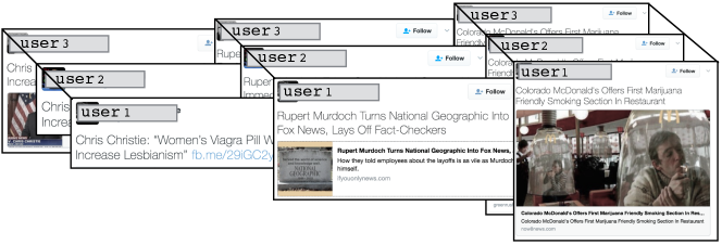
Figure 1. A group of Twitter accounts who shared the same set of fake articles.

Fake news on social media has experienced a resurgence of interest due to the recent political climate and the growing concern around its negative effect. For example, in January 2017, a spokesman for the German government stated that they “are dealing with a phenomenon of a dimension that [they] have not seen before”, referring to the proliferation of fake news (ger, 2017). Not only does it provide a source of spam in our lives, but fake news also has the potential to manipulate public perception and awareness in a major way.

Detecting misinformation on social media is an extremely important but also a technically challenging problem. The difficulty comes in part from the fact that even the human eye cannot accurately distinguish true from false news; for example, one study found that when shown a fake news article, respondents found it “‘somewhat’ or ‘very’ accurate 75% of the time”, and another found that 80% of high school students had a hard time determining whether an article was fake (Edkins, 2016; npr, 2016). In an attempt to combat the growing misinformation and confusion, several fact-checking websites have been deployed to expose or confirm stories (e.g. snopes.com). These websites play a crucial role in combating fake news, but they require expert analysis which inhibits a timely response. As a response, numerous articles and blogs have been written to raise public awareness and provide tips on differentiating truth from falsehood (McClure, 2017). While each author provides a different set of signals to look out for, there are several characteristics that are generally agreed upon, relating to the text of an article, the response it receives, and its source.

The most natural characteristic is the text of an article. Advice in the media varies from evaluating whether the headline matches the body of the article, to judging the consistency and quality of the language. Attempts to automate the evaluation of text have manifested in sophisticated natural language processing and machine learning techniques that rely on hand-crafted and data-specific textual features to classify a piece of text as true or false (Gupta et al., 2014; Ferreira and Vlachos, 2016; Ma et al., 2016; Markowitz and Hancock, 2014; Markines et al., 2009; Rubin et al., 2015). These approaches are limited by the fact that the linguistic characteristics of fake news are still not yet fully understood. Further, the characteristics vary across different types of fake news, topics, and media platforms.

A second characteristic is the response that a news article is meant to illicit. Advice columns encourage readers to consider how a story makes them feel – does it provoke either anger or an emotional response? The advice stems from the observation that fake news often contains opinionated and inflammatory language, crafted as click bait or to incite confusion (Chen et al., 2015; Rubin, 2017). For example, the New York Times cited examples of people profiting from publishing fake stories online; the more provoking, the greater the response, and the larger the profit (Maheshwari, 2016). Efforts to automate response detection typically model the spread of fake news as an epidemic on a social graph (Friggeri et al., 2014; Jin et al., 2013; Starbird et al., 2014; Kumar et al., 2016), or use hand-crafted features that are social-network dependent, such as the number of Facebook likes, combined with a traditional classifier (Castillo et al., 2011; Ma et al., 2015; Kwon et al., 2017; Wu et al., 2015; Zhao et al., 2015; Markines et al., 2009). Unfortunately, access to a social graph is not always feasible in practice, and manual selection of features is labor intensive.

A final characteristic is the source of the article. Advice here ranges from checking the structure of the url, to the credibility of the media source, to the profile of the journalist who authored it; in fact, Google has recently banned nearly 200 publishers to aid this task (Townsend, 2017). In the interest of exposure to a large audience, a set of loyal promoters may be deployed to publicize and disseminate the content. In fact, several small-scale analyses have observed that there are often groups of users that heavily publicize fake news, particularly just after its publication (Lotan, 2016; kre, 2015). For example, Figure 1 shows an example of three Twitter users who consistently promote the same fake news stories. Approaches here typically focus on data-dependent user behaviors, or identifying the source of an epidemic, and disregard the fake news articles themselves (Wang et al., 2014; Mukherjee et al., 2012).

Each of the three characteristics mentioned above has ambiguities that make it challenging to successfully automate fake news detection based on just one of them. Linguistic characteristics are not fully understood, hand-crafted features are data-specific and arduous, and source identification does not trivially lead to fake news detection. In this work, we build a more accurate automated fake news detection by utilizing all three characteristics at once: text, response, and source. Instead of relying on manual feature selection, the CSI model that we propose is built upon deep neural networks, which can automatically select important features. Neural networks also enable CSI to exploit information from different domains and capture temporal dependencies in users engagement with articles. A key property of CSI is that it explicitly outputs information both on articles and users, and does not require the existence of a social graph, domain knowledge, nor assumptions on the types and distribution of behaviors that occur in the data.

Specifically, CSI is composed of one module for each side of the activity, user and article – Figure 3(b) illustrates the intuition. The first module, called Capture, exploits the temporal pattern of user activity, including text, to capture the response a given article received. Capture is constructed as a Recurrent Neural Network (more precisely an LSTM) which receives article-specific information such as the temporal spacing of user activity on the article and a doc2vec (Le and Mikolov, 2014) representation of the text generated in this activity (such as a tweet). The second module, which we call Score, uses a neural network and an implicit user graph to extract a representation and assign a score to each user that is indicative of their propensity to participate in a source promotion group. Finally, the third module, Integrate, combines the response, text, and source information from the first two modules to classify each article as fake or not. The three module composition of CSI allows it to independently learn characteristics from both sides of the activity, combine them for a more accurate prediction and output feedback both on the articles (as a falsehood classification) and on the users (as a suspiciousness score).

Experiments on two real-world datasets demonstrate that by incorporating text, response, and source, the CSI model achieves significantly higher classification accuracy than existing models. In addition, we demonstrate that both the Capture and Score modules provide meaningful information on each side of the activity. Capture generates low-dimensional representations of news articles and users that can be used for tasks other than classification, and Score rates users by their participation in group behavior.

The main contributions can be summarized as:

1. To the best of our knowledge, we propose the first model that explicitly captures the three common characteristics of fake news, text, response, and source, and identifies misinformation both on the article and on the user side.

2. The proposed model, which we call CSI, evades the cost of manual feature selection by incorporating neural networks. The features we use capture the temporal behavior and textual content in a general way that does not depend on the data context nor require distributional assumptions.

3. Experiments on real world datasets demonstrate that CSI is more accurate in fake news classification than previous work, while requiring fewer parameters and training.

2. Related work

The task of detecting fake news has undergone a variety of labels, from misinformation, to rumor, to spam. Just as each individual may have their own intuitive definition of such related concepts, each paper adopts its own definition of these words which conflicts or overlaps both with other terms and other papers. For this reason, we specify that the target of our study is detecting news content that is fabricated, that is fake. Given the disparity in terminology, we overview existing work grouped loosely according to which of the three characteristics (text, response, and source) it considers.

There has been a large body of work surrounding text analysis of fake news and similar topics such as rumors or spam. This work has focused on mining particular linguistic cues, for example, by finding anomalous patterns of pronouns, conjunctions, and words associated with negative emotional word usage (Feng and Hirst, 2013; Markowitz and Hancock, 2014). For example, Gupta et al. (Gupta et al., 2014) found that fake news often contain an inflated number of swear words and personal pronouns. Branching off of the core linguistic analysis, many have combined the approach with traditional classifiers to label an article as true or false (Castillo et al., 2011; Ma et al., 2015; Kwon et al., 2017; Wu et al., 2015; Zhao et al., 2015; Markines et al., 2009; Ferreira and Vlachos, 2016). Unfortunately, the linguistic indicators of fake news across topic and media platform are not yet well understood; Rubin et al. (Rubin et al., 2015) explained that there are many types of fake news, each with different potential textual indicators. Thus existing works design hand-crafted features which is not only laborious but highly dependent on the specific dataset and the availability of domain knowledge to design appropriate features. To expand beyond the specificity of hand-crafted features, Ma et al. (Ma et al., 2016) proposed a model based on recurrent neural networks that uses mainly linguistic features. In contrast to (Ma et al., 2016), the CSI model we propose captures all three characteristics, is able to isolate suspicious users, and requires fewer parameters for a more accurate classification.

The response characteristic has also received attention in existing work. Outside of the fake news domain, Castillo et al. (Castillo et al., 2014) showed that the temporal pattern of user response to news articles plays an important role in understanding the properties of the content itself. From a slightly different point of view, one popular approach has been to measure the response an article received by studying its propagation on a social graph (Friggeri et al., 2014; Jin et al., 2013; Starbird et al., 2014; Kumar et al., 2016). The epidemic approach requires access to a graph which is infeasible in many scenarios. Another approach has been to utilize hand-crafted social-network dependent behaviors, such as the number of Facebook likes, as features in a classifier (Castillo et al., 2011; Ma et al., 2015; Kwon et al., 2017; Wu et al., 2015; Zhao et al., 2015; Markines et al., 2009). As with the linguistic features, these works require feature-engineering which is laborious and lacks generality.

The final characteristic, source, has been studied as the task of identifying the source of an epidemic on a graph (Wang et al., 2014; Luo et al., 2013; Zhu and Ying, 2016), or isolating bots based on certain documented behaviors (Chavoshi et al., 2016; Varol et al., 2017). Another approach identifies group anomalies. Early work in group anomaly detection assumed that the groups were known a priori, and the goal was to detect which of them were anomalous (Mukherjee et al., 2012). Such information is not feasible in practice, hence later works propose variants of mixtures models for the data, where the learned parameters are used to identify the anomalous groups (Xiong et al., 2011a; Xiong et al., 2011b). Muandet et al. (Muandet and Schölkopf, 2013) took a similar approach by combining kernel embedding with an SVM classifier. Most recently, Yu et al. (Yu et al., 2015) proposed a unified hierarchical Bayes model to infer the groups and detect group anomalies simultaneously. There has also been a strong line of work surrounding detecting suspicious user behavior of various types; a nice overview is given in (Jiang et al., 2016). Of this line, the most related is the CopyCatch model proposed in (Beutel et al., 2013), which identifies temporal bipartite cores of user activity on pages. In contrast to existing works, the CSI model we propose can identify group anomalies as well as the core behaviors they are responsible for (fake news). The model does not require group information as input, does not make assumptions about a particular distribution, and learns a representation and score for each user.

In contrast to the vast array of work highlighted here, the CSI model we propose does not rely on hand-crafted features, domain knowledge, or distributional assumptions, offering a more general modeling of the data. Further, CSI captures all three characteristics and outputs both a classification of articles, a scoring of users, and representations of both users and articles that can be used for in separate analysis.

3. Problem

In this section we first lay out preliminaries, and then discuss the context of fake news which we address.

Preliminaries: We consider a series of temporal engagements that occurred between $n$ users with $m$ news-articles over time $[1,T]$. Each engagement between a user $u_{i}$ and an article $a_{j}$ at time $t$ is represented as $e_{ijt}=(u_{i},a_{j},t)$. In particular, in our setting, an engagement is composed of textual information relayed by the user $u_{i}$ about article $a_{j}$, at time $t$; for example, a tweet or a Facebook post. Figure 2 illustrates the setting. In addition, we assume that each news article is associated with a label $L(a_{j})=0$ if the news is true, and $L(a_{j})=1$ if it is false. Throughout we will use italic characters $x$ for scalars, bold characters h for vectors, and capital bold characters W for matrices.

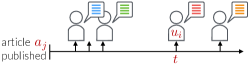
Figure 2. Temporal engagements of users with articles.

Goal: While the overarching theme of this work is fake news detection, the goal is two fold (1) accurately classify fake news, and (2) identify groups of suspicious users. In particular, given a temporal sequence of engagements $E=\{e_{ijt}=(u_{i},a_{j},t)\}$, our goal is to produce a label $\hat{L}(a_{j})\in[0,1]$ for each article, and a suspiciousness score $s_{i}$ for each user. To do this we encapsulate the text, response, and source characteristics in a model and capture the temporal behavior of both parties, users and articles, as well as textual information exchanged in the activity. We make no assumptions on the distribution of user behavior, nor on the context of the engagement activity.

4. Model

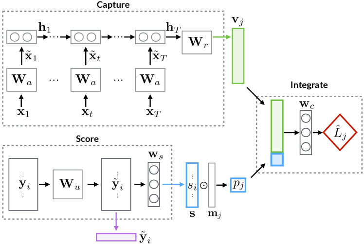
(a) The CSI model specification. The Capture module depicts the LSTM for a single article $a_{j}$, while the Score module operates over all users. The output of Score is then filtered to be relevant to $a_{j}$.

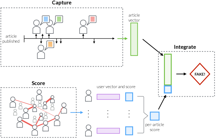
(b) Intuition behind CSI. Here, Capture receives the temporal series of engagements, and Score is fed an implicit user graph constructed from the engagements over all articles in the data.

Figure 3. An illustration of the proposed CSI model.

In this section, we give the details of the proposed model, which we call CSI. The model consists of two main parts, a module for extracting temporal representation of news articles, and a module for representing and scoring the behavior of users. The former captures the response characteristic described in Section 1 while incorporating text, and the latter captures the source characteristic. Specifically, CSI is composed of the following three parts, the specification and intuition of which is shown in Figure 3:

1. Capture: To extract temporal representations of articles we use a Recurrent Neural Network (RNN). Temporal engagements are stored as vectors and are fed into the RNN which produces an output a representation vector $\textbf{v}_{j}$.

2. Score: To compute a score $s_{i}$ and representation $\tilde{\textbf{y}}_{i}$, user-features are fed into a fully connected layer and a weight is applied to produce the scores vectors s.

3. Integrate: The outputs of the two modules are concatenated and the resultant vector is used for classification.

With the first two modules, Capture and Score, the CSI model extracts representations of both users and articles as low-dimensional vectors; these representations are important for the fake news task, but can also be used for independent analysis of users and articles. In addition, Score produces a score for each user as a compact version of the vector. The Integrate module then combines the article representations with the user scores for an ultimate prediction of the veracity of an article. In the sections that follow, we discuss the details of each module.

4.1. Capture news article representation

In the first module, we seek to capture the pattern of temporal engagement of users with an article $a_{j}$ both in terms of the frequency and distribution. In other words, we wish to capture not only the number of users that engaged with $a_{j}$ in Figure 3(b), but also how the engagements were spaced over time. Further, we incorporate textual information naturally available with the engagement, such as the text of a tweet, in a general and automated way.

As the core of the first module, we use a Recurrent Neural Network (RNN), since RNNs have been shown to be effective at capturing temporal patterns in data and for integrating different sources of information. A key component of Capture is the choice of features used as input to the cells for each article. Our feature vector $\textbf{x}_{t}$ has the following form:

$$\textbf{x}_{t}=(\eta,\Delta t,\textbf{x}_{u},\textbf{x}_{\tau})$$

The first two variables, $\eta$ and $\Delta t$, capture the temporal pattern of engagement an article receives with two simple, yet powerful quantities: the number of engagements $\eta$, and the time between engagements $\Delta t$. Together, $\eta$ and $\Delta t$ provide a general of measure the frequency and distribution of the response an article received. Next, we incorporate source by adding a user feature vector $\textbf{x}_{u}$ that is global and not specific to a given article. In line with existing literature on information retrieval and recommender systems (Leskovec et al., 2014), we construct the binary incidence matrix of which articles a user engaged with, and apply the Singular Value Decomposition (SVD) to extract a lower-dimensional representation for each $u_{i}$. Finally, a vector $\textbf{x}_{\tau}$ is included which carries the text characteristic of an engagement with a given article $a_{j}$. To avoid hand-crafted textual feature selection for $\textbf{x}_{\tau}$, we use doc2vec (Le and Mikolov, 2014) on the text of each engagement. Further technical details will be explained in Section 5.

Since the temporal and textual features come from different domains, it is not desirable to incorporate them into the RNN as raw input. To standardize the input features, we insert an embedding layer between the raw features $\textbf{x}_{t}$ and the inputs $\tilde{\textbf{x}}_{t}$ of the RNN. This embedding layer is a fully connected layer as following:

$$\tilde{\textbf{x}}_{t}=\text{tanh}(\textbf{W}_{a}\textbf{x}_{t}+\textbf{b}_{a})$$

where $\textbf{W}_{a}$ is a weight matrix applied to the raw features $\textbf{x}_{t}$ at time $t$ and $\textbf{b}_{a}$ is a bias vector. Both $\textbf{W}_{a}$ and $\textbf{b}_{a}$ are the fixed for all $\textbf{x}_{t}$. To capture the temporal response of users to an article, we construct the Capture module using a Long Short-Term Memory (LSTM) model because of its propensity for capturing long-term dependencies and its flexibility in processing inputs of variable lengths. For the sake of brevity we do not discuss the well-established LSTM model here, but refer the interested reader to (Hüsken and Stagge, 2003) for more detail.

What is important for our discussion is that in the final step of the LSTM, $\tilde{\textbf{x}}_{T}$ is fed as input and the last hidden state $\textbf{h}_{T}$ is passed to the fully connected layer. The result is a vector:

$$\textbf{v}_{j}=\text{tanh}(\textbf{W}_{r}\textbf{h}_{T}+\textbf{b}_{r})$$

This vector serves as a low dimension representation of the temporal pattern of engagements a given article $a_{j}$ received – capturing both the response and textual characteristics. The vectors $\textbf{v}_{j}$ will be fed to the Integrate module for article classification, but can also be used for stand-alone analysis of articles.

Partitioning: In principle, the feature vector $\textbf{x}_{t}$ associated with each engagement can be considered as an input into a cell; however, this would be highly inefficient for large data. A more efficient approach is to partition a given sequence by changing the granularity, and using an aggregate of each partition (such as an average) as input to a cell. Specifically, the feature vector for article $a_{j}$ at partition $t$ has the following form: $\eta$ is the number of engagements that occurred in partition $t$, $\Delta t$ holds the time between the current and previous non-empty partitions, $\textbf{x}_{u}$ is the average of user-features over users $u_{i}$ that engaged with $a_{j}$ during $t$, and $\tau$ is the textual content exchanged during $t$.

4.2. Score users

In the second module, we wish to capture the source characteristic present in the behavior of users. To do this, we seek a compact representation that will have the same (small) dimension for every article (since it will ultimately be used in the Integrate module). Given a set of user features, we first apply a fully connected layer to extract vector representations of each user as follows:

$$\tilde{\textbf{y}}_{i}=\text{tanh}(\textbf{W}_{u}{\textbf{y}_{i}}+\textbf{b}_{u})$$

where $\textbf{W}_{u}$ is the weight matrix and $\textbf{b}_{u}$ is the bias; $L2$-regularization is used on $\textbf{W}_{u}$ with parameter $\lambda$. This results in a vector representation $\tilde{\textbf{y}}_{i}$ for each user $u_{i}$ that is learned jointly with the Capture module. To aggregate this information, we apply a weight vector $\textbf{w}_{s}$ to produce a scalar score $s_{i}$ for each user as:

$$s_{i}=\sigma(\textbf{w}^{\top}_{s}\cdot\tilde{\textbf{y}}_{i}+{b}_{s})$$

with ${b}_{s}$ as the bias of a fully connected layer, and $\sigma$ as the sigmoid function. The set of $s_{i}$ forms the vector s of user scores.

In principle, user features can be constructed using information from the users social network profile. Since we wish to capture the source characteristic, we construct a weighted user graph where an edge denotes the number of articles with which two users have both engaged. Users who engage in group behavior will correspond to dense blocks in the adjacency matrix. Following the literature, we apply the SVD to the adjacency matrix and extract a lower-dimensional feature $\textbf{y}_{i}$ for each user, ultimately obtaining $(s_{i},\tilde{\textbf{y}}_{i})$ for each user $u_{i}$.

By constructing the Score module in this way, CSI is able to jointly learn from the two sides of the engagements while extracting information that is meaningful to the source characteristic. As with the Capture module, the vector $\tilde{\textbf{y}}_{i}$ can be used for stand-alone analysis of the users.

4.3. Integrate to classify

Each of the Capture and Score modules outputs information on articles and users with respect to the three characteristics of interest. In order to incorporate the two sources of information, we propose a third module as the final step of CSI in which article representations $\textbf{v}_{j}$ are combined with the user scores $s_{i}$ to produce a label prediction $\hat{L}_{j}$ for each article.

To integrate the two modules, we apply a mask $\textbf{m}_{j}$ to the vector s that selects only the entries $s_{i}$ whose corresponding user $u_{i}$ engaged with a given article $a_{j}$. These values are average to produce $p_{j}$ which captures the suspiciousness score of the users that engage with the specific article $a_{j}$. The overall score $p_{j}$ is concatenated with $\textbf{v}_{j}$ from Capture, and the resultant vector $\textbf{c}_{j}$ is fed into the last fully connected layer to predict the label $\hat{L}_{j}$ of article $a_{j}$.

$$\hat{L}_{j}=\sigma(\textbf{w}^{\top}_{c}\textbf{c}_{j}+{b}_{c})$$

This integration step enables the modules to work together to form a more accurate prediction. By jointly training the CSI with the Capture and Score modules, the model learns both user and article information simultaneously. At the same time, the CSI model generates information on articles and users that captures different important characteristics of the fake news problem, and combines the information for an ultimate prediction.

Training: The loss function for training CSI is specified as:

$$Loss=-\frac{1}{N}\sum_{j=1}^{N}\left[L_{j}\log\hat{L}_{J}+(1-L_{j})\log(1-\hat{L}_{j})\right]+\frac{\lambda}{2}||\textbf{W}_{u}||^{2}_{2}$$

where $L_{j}$ is a the ground-truth label. To reduce overfitting in CSI, random units in $\textbf{W}_{a}$ and $\textbf{W}_{r}$ are dropped out for training. Under these constraints, the parameters in Capture, Score, and Integrate are jointly trained by back-propagation.

4.4. Generality

We have presented the CSI model in the context of fake news; however, our model can be easily generalized to any dataset. Consider a set of engagements between an actor $q_{i}$ and a target $r_{j}$ over time $t\in[0,T]$, in other words, the article in Figure 3(b) is a target and each user is an actor. The Capture module can be used to capture the temporal patterns of engagements exhibited on targets by actors, and Score can be used to extract a score and representation of each actor $q_{i}$ that captures the participation in group behavior. Finally, Integrate combines the first two modules to enhance the prediction quality on targets. For example, consider users accessing a set of databases. The Capture module can identify databases which received an unusual pattern of access, and Score can highlight users that were likely responsible. In addition, the flexibility of CSI allows for integration of additional domain knowledge.

5. Experiments

	Twitter	Weibo
# Users	233,719	2,819,338
# Articles	992	4,664
# Engagements	592,391	3,752,459
# Fake articles	498	2,313
# True articles	494	2,351
Avg $T$ per article (hours)	1,983	1,808

Table 1. Statistics of the datasets.

In this section, we demonstrate the quality of CSI on two real world datasets. In the main set of experiments, we evaluate the accuracy of the classification produced by CSI. In addition, we investigate the quality of the scores and representations produced by the Score module and show that they are highly related to the score characteristic. Finally, we show the robustness of our model when labeled data is limited and investigate temporal behaviors of suspicious users.

Datasets In order to have a fair comparison, we use two real-world social media datasets that have been used in previous work, Twitter and Weibo (Ma et al., 2016). To date, these are the only publicly available datasets that include all three characteristics: response, text, and user information. Each dataset has a number of articles with labels $L(a_{j})$; in Twitter the articles are news stories, and in Weibo they are discussion topics. Each article also has a set of engagements (tweets) made by a user $u_{i}$ at time $t$. A summary of the statistics is listed in Table 1.

5.1. Model setup

We first describe the details of two important components in CSI: 1) how to obtain the temporal partitions discussed in Section 4 and 2) the specific features for each dataset.

Partitioning: As mentioned in Section 4, treating each time-stamp as its own input to a cell can be extremely inefficient and can reduce utility. Hence, we propose to partition the data into segments, each of which will be an input to a cell. We apply a natural partitioning by changing the temporal granularity from seconds to hours.

Hyperparameters: We use cross-validation to set the regularization parameter for the loss function in Section 4.3 to $\lambda=0.01$, the dropout probability as $0.2$, the learning rate to $0.001$, and use the Adam optimizer.

Features: Recall from Section 4 that Capture operates on $\textbf{x}_{t}=(\eta,\Delta t,\textbf{x}_{u},\textbf{x}_{\tau})$ – temporal, user, and textual features. To apply doc2vec(Le and Mikolov, 2014) to the Weibo data, we first apply Chinese text segmentation. To extract $\textbf{x}_{u}$, we apply the SVD with rank $20$ for Twitter and $10$ for Weibo, resulting in $122$ dimensional $\textbf{x}_{t}$ for Twitter and $112$ for Weibo. (SVD dimension chosen using the Scree plot.) We then set the embedding dimension so that each $\tilde{\textbf{x}}_{t}$ has dimension $100$. The SVD rank for $\textbf{x}_{i}$ for Score is $50$ for both datasets , and the dimension of $\textbf{W}_{u}$ is 100.

	Twitter		Weibo
	Accuracy	F-score	Accuracy	F-score
DT-Rank	0.624	0.636	0.732	0.726
DTC	0.711	0.702	0.831	0.831
SVM-TS	0.767	0.773	0.857	0.861
LSTM-1	0.814	0.808	0.896	0.913
GRU-2	0.835	0.830	0.910	0.914
CI	0.847	0.846	0.928	0.927
CI-t	0.854	0.848	0.939	0.940
CSI	0.892	0.894	0.953	0.954

Table 2. Comparison of detection accuracy on two datasets

5.2. Fake news classification accuracy

In the main set of experiments, we use two real-world datasets, Twitter and Weibo, to compare the proposed CSI model with five state-of-the-art models that have been used for similar classification tasks and were discussed in Section 2: SVM-TS (Ma et al., 2015) , DT-Rank (Zhao et al., 2015), DTC (Castillo et al., 2011) , LSTM-1 (Ma et al., 2016), and GRU-2 (Ma et al., 2016). Further, to evaluate the utility of different features included in the model, we consider CI as the CSI model using only textual features $\textbf{x}_{t}=(\textbf{x}_{\tau})$, CI-t as using textual and temporal features $\textbf{x}_{t}=(\eta,\Delta t,\textbf{x}_{\tau})$, and finally CSI using textual, temporal, and user features. Since the first two do not incorporate user information, we omit the S from the name. All RNN-based models including LSTM-1 and GRU-2 were implemented with Theano and tested with Nvidia Tesla K40c GPU. The AdaGrad algorithm is used as an optimizer for LSTM-1 and GRU-2 as per (Ma et al., 2016). For CSI, we used the Adam algorithm.

Table 2 shows the classification results using 80% of entire data as training samples, 5% to tune parameters, and the remaining 15% for testing; we use 5-fold cross validation. This division is chosen following previous work for fair comparison, and will be studied in later sections. We see that CSI outperforms other models in both accuracy and F-score. Specifically, CI shows similar performance with GRU-2 which is a more complex 2-layer stacked network. This performance validates our choice of capturing fundamental temporal behavior, and demonstrates how a simpler structure can benefit from better features and partitioning. Further, it shows the benefit of utilizing doc2vec over simple tf-idf.

Next, we see that CI-t exhibits an improvement of more than $1\%$ in both accuracy and F-score over CI. This demonstrated that while linguistic features may carry some temporal properties, the frequency and distribution of engagements caries useful information in capturing the difference between true and fake news.

Finally, CSI gives the best performance over all comparison models and versions. We see that integrating user features boosts the overall numbers up to 4.3% from GRU-2. Put together, these results demonstrate that CSI successfully captures and leverages all three characteristics of text, response, and source, for accurately classifying fake news.

5.3. Model complexity

In practice, the availability of labeled examples of true and fake news may be limited, hence, in this section, we study the usability of CSI in terms of the number of parameters and amount of labeled training samples it requires.

Although CSI is based on deep neural networks, the compact set of features that Capture utilizes results in fewer required parameters than other models. Furthermore, the user relations in Score can deliver condensed representations which cannot be captured by an RNN, allowing CSI to have less parameters than other RNN-based models. In particular, the model has on the order of $52K$ parameters, whereas GRU-2 has $621K$ parameter.

To study the number of labeled samples CSI relies on, we study the accuracy as a function of the training set size. Figure 4 shows that even if only 10% training samples are available, CSI can show comparable performance with GRU-2; thus, the CSI model is lighter and can be trained more easily with fewer training samples.

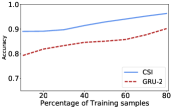
(a) Twitter

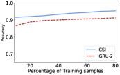
(b) Weibo

Figure 4. Accuracy vs. the percentage of training samples.

5.4. Interpreting user representations

In this section, we analyze the output of Score which is a score $s_{i}$ and a representation $\tilde{\textbf{y}}_{i}$ for every user. Since the available data does not have ground-truth labels on users, we perform a qualitative evaluation of the information contained in $(s_{i},\tilde{\textbf{y}}_{i})$ with respect to the source characteristic of fake news.

Although we lack user-labels, the dataset still contains information that can be used as a proxy. In particular, we want to evaluate whether $(s_{i},\tilde{\textbf{y}}_{i})$ captures the suspicious behavior of users in terms promotion of fake news and group behavior. For the former, a reasonable proxy is the fraction of fake news a user engages with, denoted $\ell_{i}\in[0,1]$ with $0.0$ meaning the user has never reacted to fake news, and $1.0$ meaning the engagements are exclusively with fake news. In addition, we consider the corresponding scores for articles as the average over users, namely $p_{j}$ is the average of $s_{i}$ and $\lambda_{j}$ is the average of $\ell_{i}$ over $u_{i}$ that engaged with $a_{j}$.

To test the extent to which $(s_{i},\tilde{\textbf{y}}_{i})$ capture $\ell_{i}$, we compute the correlation between the two measures across users; Table 3 shows the Pearson correlation coefficient and significance. For both datasets and on both sides of the user-article engagement, we find a statistically significant positive relationship between the two scores. Results are consistent for the Spearman coefficient and for ordinary least squares regression(OLS). In addition, Figures 5(a) and 5(b) show the distribution of $\ell_{i}$ among a subset of users with highest and lowest $s_{i}$. Most of the users who were assigned a high $s_{i}$ by CSI (marked as most suspicious) have $\ell_{i}$ close to $1$, while those with low $s_{i}$ have low $\ell_{i}$. Altogether, the results demonstrate that $s_{i}$ and $p_{j}$ hold meaningful information with respect to user levels of engagement with fake news.

	User	Article
Twitter	$0.525$***	$0.671$***
Weibo	$0.485$***	$0.646$***

Table 3. Correlation between $\ell_{i}$ and $\tilde{\textbf{y}}_{i}$ with statistical significance as *$<0.1$, **$<0.05$, and ***$<0.01$.

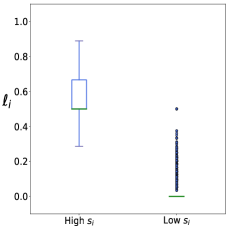
(a) Twitter

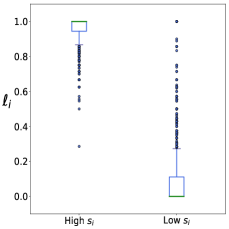
(b) Weibo

Figure 5. Distribution of $\ell_{i}$ over users marked as high and low suspicion according to the s vector produce by CSI.

To investigate the relation of $\tilde{\textbf{y}}_{i}$ to $\ell_{i}$, we regress the cosine distance between $\tilde{\textbf{y}}_{i}$ and $\tilde{\textbf{y}}_{i^{\prime}}$ against the difference between $\ell_{i}$ and $\ell_{i^{\prime}}$ for each pair of users $(i,i^{\prime})$. Consistent with results for $s_{i}$, we find a positive correlation of $0.631$ for Twitter and $0.867$ for Weibo, both of which are statistically significant at the $1\%$ level. Further, we visualize the space of user representations by projecting a sample of the vectors $\tilde{\textbf{y}}_{i}$ onto the first and second singular vectors $\mu_{1}$ and $\mu_{2}$ of the matrix of $\tilde{\textbf{y}_{i}}$’s. Figure 6 shows the projection for both datasets, where each point corresponds to a user $u_{i}$ and is colored according to $\ell_{i}$. We see that the space exhibits a strong separation between users with extreme $\ell_{i}$, suggesting that the vectors $\tilde{\textbf{y}}_{i}$ offer a good latent representation of user behavior with respect to fake news and can be used for deeper user analysis.

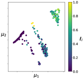
(a) Twitter users

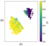
(b) Weibo users

Figure 6. Projection of user vectors $\textbf{z}_{j}$.

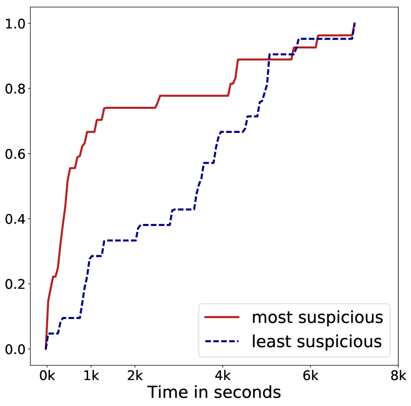
(a) Fake news on Twitter

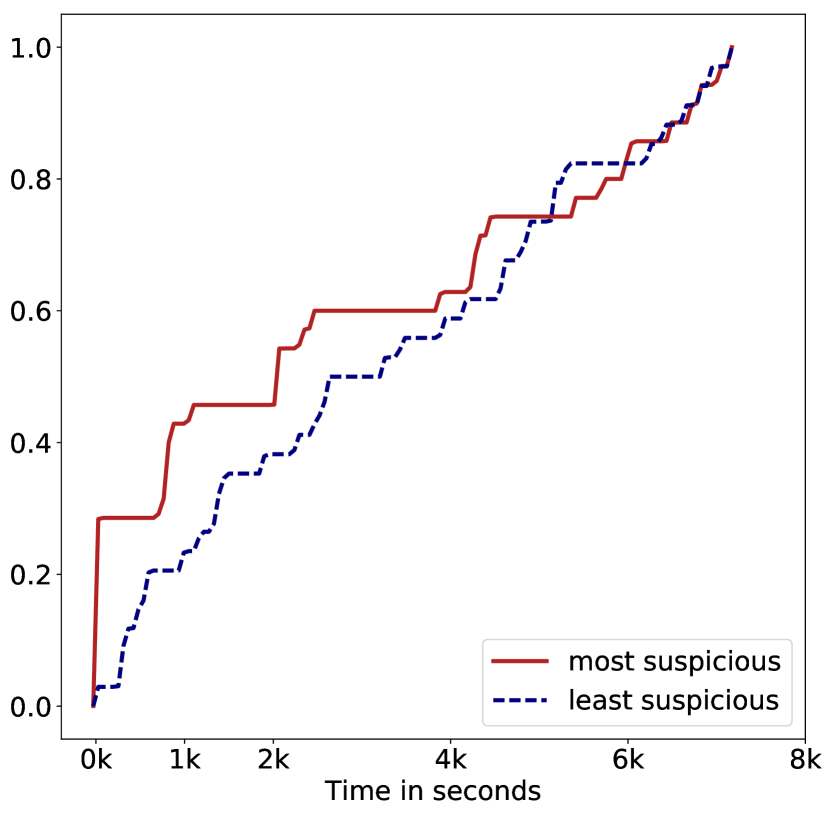
(b) True news on Twitter

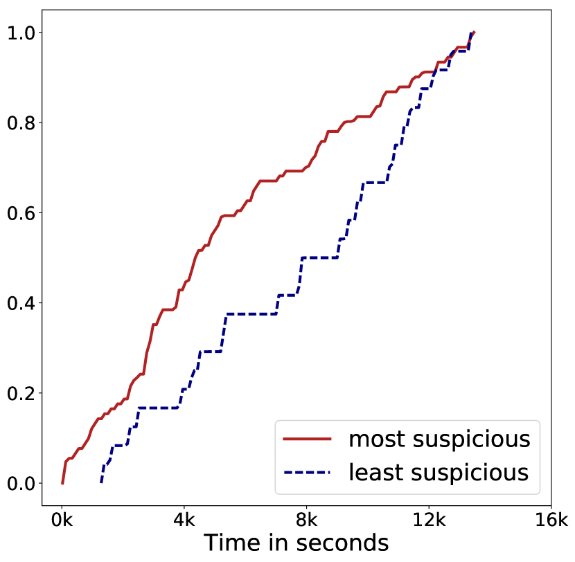
(c) Fake news on Weibo

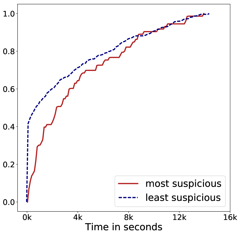
(d) True news on Weibo

Figure 7. Distribution (CDF) of user lags on Twitter and Weibo.

Next, we analyze the propensity of $(s_{i},\tilde{\textbf{y}}_{i})$ to capture group behavior. We construct an implicit user graph by adding an edge between users who have engaged with the same article, and by analyze the clustering of users in the graph. We apply the BiMax algorithm proposed by Prelić et al. (Prelić et al., 2006) to search for biclusters in the adjacency matrix. We find that for both datasets, users with large $\ell_{i}$ participate in more and larger biclusters than those with low $\ell_{i}$. Further, biclusters for users with large $\ell_{i}$ are formed largely with fake news articles, while those for low $\ell_{i}$ are largely with true news.

This suggests that suspicious users exhibit the source characteristic with respect to fake news. In addition, for each pair of users $(u_{i},u_{i^{\prime}})$ we compute the Jaccard distance between the set of articles they interacted with. We compute the correlation between this quantity and $|s_{i}-s_{i^{\prime}}|$ as well as the cosine distance between $\tilde{\textbf{y}}_{i}$ and $\tilde{\textbf{y}}_{i^{\prime}}$. For the former we find a correlation of $0.36$ for Twitter and $0.21$ for Weibo, and for the latter we find $0.30$ for Twitter and $0.16$ for Weibo. All results are significant at the $1\%$ level, with Spearman correlation and OLS giving consistent results.

Overall, despite lack of ground-truth labels on users, our analysis demonstrates that the Score module captures meaningful information with respect to the the source characteristic. The user score $s_{i}$ provides the model with an indication of the suspiciousness of user $u_{i}$ with respect to group behavior and fake news engagement. Further, the $\tilde{\textbf{y}}_{i}$ vector provides a representation of each user that can be used for deeper analysis of user behavior in the data.

5.5. Characterizing user behavior

In this section, we ask whether the users marked as suspicious by CSI have any characteristic behavior. Using the $s_{i}$ scores of each user we select approximately $25$ users from the most suspicious groups, and the same amount from the least suspicious group.

We consider two properties of user behavior: (1) the lag and (2) the activity. To measure lag for each user, we compute the lag in time between time between an article’s publication, and when the user first engaged with it. We then plot the distribution of user lags separated by most and least suspicious, and true and fake news. Figure 7 shows the CDF of the results. Immediately we see that the most suspicious users in each dataset are some of the first to promote the fake content – supporting the source characteristic. In contrast, both types of users act similarly on real news.

Next, we measure the user activity as the time between engagements user $u_{i}$ had with a particular article $a_{j}$. Figure 8 shows the CDF of user activity. We see that on both datasets, suspicious users often have bursts of quick engagements with a given article; this behavior differs more significantly from the least suspicious users on fake news than it does on true news. Interestingly, the behavior of suspicious users on Twitter is similar on fake and true news, which may demonstrate a sophistication in fake content promotion techniques. Overall, these distributions show that the combination of temporal, textual, and user features in $\textbf{x}_{t}$ provides meaningful information to capture the three key characteristics, and for CSI to distinguishing suspicious users.

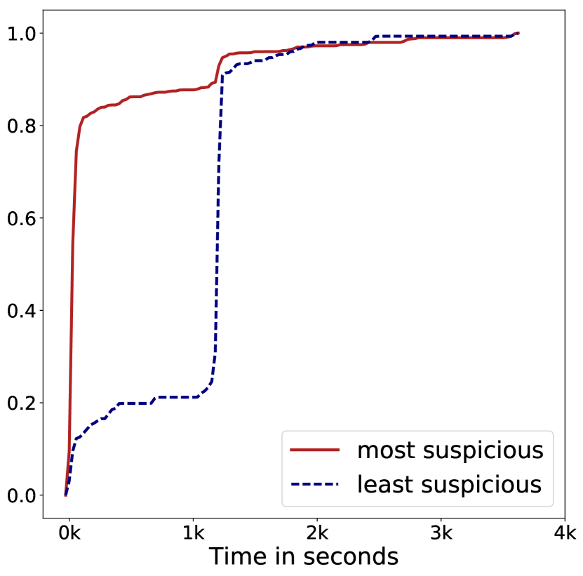
(a) Fake news on Twitter

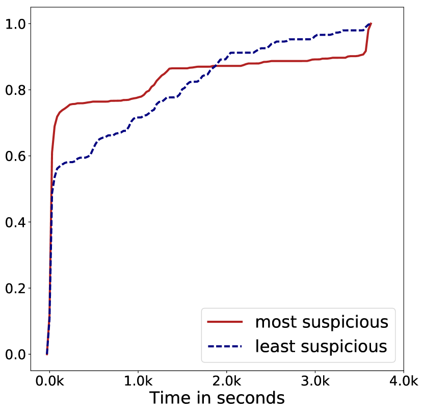
(b) True news on Twitter

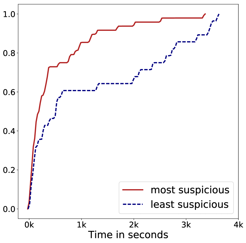
(c) Fake news on Weibo

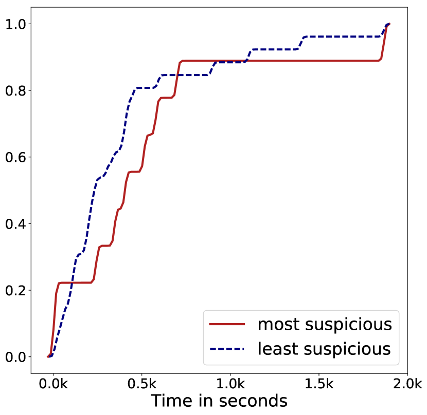
(d) True news on Weibo

Figure 8. Distribution (CDF) of user activity on Twitter and Weibo.

5.6. Utilizing temporal article representations

In this section, we investigate the vector $\textbf{v}_{j}$ that is the output of Capture for each article $a_{j}$. Intuitively, these vectors are a low-dimensional representation of the temporal and textual response an article has received, as well as the types of users the response has come from. In a general sense, the output of an LSTM has been used for a variety of tasks such as machine translation (Sutskever et al., 2014), question answering (Wang and Nyberg, 2015), and text classification (Lee and Dernoncourt, 2016). Hence, in the context of this work it is natural to wondering whether these vectors can be used for deeper insight into the space of articles.

As an example, we consider applying Spectral Clustering for a more fine-grained partition than two classes. We consider the set of $\textbf{v}_{j}$ associated with the test set of Twitter and Weibo articles, and set $k=5$ clusters according to the elbow curve. Figure 9 shows the results in the space of the first two singular vectors ($\mu_{1}$ and $\mu_{2}$) of the matrix formed by the vectors $\textbf{v}_{j}$ for each respective dataset, with one color for each cluster.

Table 4 shows the breakdown of true and false articles in each cluster. We can see that the results gives a natural division both among true and fake articles. For example, on the Twitter datasets, while both C2 and C4 are composed of mostly fake news, we can see that the projections of their temporal representation are quite separated. This separation suggests that there may be different types of fake news which exhibit slightly different signals in the text, response, and source characteristics, for example, satire and spam. The Weibo data shows two poles: C1 in the top left corresponds largely to true news, while C2 and C4 captures different types of fake news. Meanwhile, C3 and C5 which are spread across the middle, have more mixed membership.

In the context of the general framework described in Section 4, the results show that the $\textbf{v}_{j}$ vectors produced by the Capture module offer insight into the population of users with respect to their behavior towards fake news. Aside from the classification output of the model, the representations can be used stand-alone for gaining insight about targets (articles) in the data.

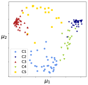
(a) Twitter

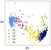
(b) Weibo

Figure 9. Article clustering with $\textbf{v}_{j}$ on Twitter and Weibo.

Twitter				Weibo
Cluster	True	False		Cluster	True	False
1	16	17		1	362	5
2	5	33		2	16	326
3	46	2		3	45	10
4	3	16		4	0	72
5	11	8		5	28	37

Table 4. Cluster statistics for Twitter and Weibo for Figure 9.

6. Conclusion

In this work, we study the timely problem of fake news detection. While existing work has typically addressed the problem by focusing on either the text, the response an article receives, or the users who source it, we argue that it is important to incorporate all three. We propose the CSI model which is composed of three modules. The first module, Capture, captures the abstract temporal behavior of user encounters with articles, as well as temporal textual and user features, to measure response as well as the text. The second component, Score, estimates a source suspiciousness score for every user, which is then combined with the first module by Integrate to produce a predicted label for each article.

The separation into modules allows CSI to output a prediction separately on users and articles, incorporating each of the three characteristics, meanwhile combining the information for classification. Experiments on two real-world datasets demonstrate the accuracy of CSI in classifying fake news articles. Aside from accurate prediction, the CSI model also produces latent representations of both users and articles that can be used for separate analysis; we demonstrate the utility of both the extracted representations and the computed user scores.

The CSI model is general in that it does not make assumptions on the distribution of user behavior, on the particular textual context of the data, nor on the underlying structure of the data. Further, by utilizing the power of neural networks, we incorporate different sources of information, and capture the temporal evolution of engagements from both parties, users and articles. At the same time, the model allows for easy incorporation of richer data, such as user profile information, or advanced text libraries. Overall our work demonstrates the value in modeling the three intuitive and powerful characteristics of fake news.

Despite encouraging results, fake news detection remains a challenging problem with many open questions. One particularly interesting direction would be to build models that incorporate concepts from reinforcement learning and crowd sourcing. Including humans in the learning process could lead to more accurate and, in particular, more timely predictions.

References

- (1)
- kre (2015) 2015. Social Network Analysis Reveals Full Scale of Kremlin’s Twitter Bot Campaign. (April 2015). globalvoices.org/2015/04/02/analyzing-kremlin-twitter-bots/
- npr (2016) 2016. Students Have ’Dismaying’ Inability To Tell Fake News From Real, Study Finds. (November 2016). www.npr.org/sections/thetwo-way/2016/11/23/503129818/study-finds-students-have-dismaying-inability-to-tell-fake-news-from-real
- ger (2017) 2017. Germany investigating unprecedented spread of fake news online. (January 2017). www.theguardian.com/world/2017/jan/09/germany-investigating-spread-fake-news-online-russia-election
- Beutel et al. (2013) Alex Beutel, Wanhong Xu, Venkatesan Guruswami, Christopher Palow, and Christos Faloutsos. 2013. Copycatch: stopping group attacks by spotting lockstep behavior in social networks. In Proceedings of the 22nd international conference on World Wide Web. ACM, 119–130.
- Castillo et al. (2014) Carlos Castillo, Mohammed El-Haddad, Jürgen Pfeffer, and Matt Stempeck. 2014. Characterizing the life cycle of online news stories using social media reactions. In Proceedings of the 17th ACM conference on Computer supported cooperative work & social computing. ACM, 211–223.
- Castillo et al. (2011) Carlos Castillo, Marcelo Mendoza, and Barbara Poblete. 2011. Information credibility on twitter. In Proceedings of the 20th international conference on World wide web. ACM, 675–684.
- Chavoshi et al. (2016) Nikan Chavoshi, Hossein Hamooni, and Abdullah Mueen. 2016. DeBot: Twitter Bot Detection via Warped Correlation. 2016 IEEE 16th International Conference on Data Mining (ICDM) (2016), 817–822.
- Chen et al. (2015) Yimin Chen, Niall J Conroy, and Victoria L Rubin. 2015. Misleading online content: Recognizing clickbait as false news. In Proceedings of the 2015 ACM on Workshop on Multimodal Deception Detection. ACM, 15–19.
- Edkins (2016) Brett Edkins. 2016. Americans Believe They Can Detect Fake News. Studies Show They Can’t. (December 2016). www.forbes.com/sites/brettedkins/2016/12/20/americans-believe-they-can-detect-fake-news-studies-show-they-cant/
- Feng and Hirst (2013) Vanessa Wei Feng and Graeme Hirst. 2013. Detecting Deceptive Opinions with Profile Compatibility.. In IJCNLP. 338–346.
- Ferreira and Vlachos (2016) William Ferreira and Andreas Vlachos. 2016. Emergent: a novel data-set for stance classification. In Proceedings of the 2016 Conference of the North American Chapter of the Association for Computational Linguistics: Human Language Technologies. ACL.
- Friggeri et al. (2014) Adrien Friggeri, Lada A Adamic, Dean Eckles, and Justin Cheng. 2014. Rumor Cascades.. In ICWSM.
- Gupta et al. (2014) Aditi Gupta, Ponnurangam Kumaraguru, Carlos Castillo, and Patrick Meier. 2014. Tweetcred: Real-time credibility assessment of content on twitter. In International Conference on Social Informatics. Springer, 228–243.
- Hüsken and Stagge (2003) Michael Hüsken and Peter Stagge. 2003. Recurrent neural networks for time series classification. Neurocomputing 50 (2003), 223–235.
- Jiang et al. (2016) Meng Jiang, Peng Cui, and Christos Faloutsos. 2016. Suspicious behavior detection: Current trends and future directions. IEEE Intelligent Systems 31, 1 (2016), 31–39.
- Jin et al. (2013) Fang Jin, Edward Dougherty, Parang Saraf, Yang Cao, and Naren Ramakrishnan. 2013. Epidemiological modeling of news and rumors on twitter. In Proceedings of the 7th Workshop on Social Network Mining and Analysis. ACM, 8.
- Kumar et al. (2016) Srijan Kumar, Robert West, and Jure Leskovec. 2016. Disinformation on the web: Impact, characteristics, and detection of wikipedia hoaxes. In Proceedings of the 25th International Conference on World Wide Web. International World Wide Web Conferences Steering Committee, 591–602.
- Kwon et al. (2017) Sejeong Kwon, Meeyoung Cha, and Kyomin Jung. 2017. Rumor Detection over Varying Time Windows. PLOS ONE 12, 1 (2017), e0168344.
- Le and Mikolov (2014) Quoc V Le and Tomas Mikolov. 2014. Distributed Representations of Sentences and Documents.. In ICML, Vol. 14. 1188–1196.
- Lee and Dernoncourt (2016) Ji Young Lee and Franck Dernoncourt. 2016. Sequential short-text classification with recurrent and convolutional neural networks. arXiv preprint arXiv:1603.03827 (2016).
- Leskovec et al. (2014) Jure Leskovec, Anand Rajaraman, and Jeffrey David Ullman. 2014. Mining of massive datasets. Cambridge University Press.
- Lotan (2016) Gilad Lotan. 2016. Fake News Is Not the Only Problem. (November 2016). points.datasociety.net/fake-news-is-not-the-problem-f00ec8cdfcb
- Luo et al. (2013) Wuqiong Luo, Wee Peng Tay, and Mei Leng. 2013. Identifying infection sources and regions in large networks. IEEE Transactions on Signal Processing 61, 11 (2013), 2850–2865.
- Ma et al. (2016) Jing Ma, Wei Gao, Prasenjit Mitra, Sejeong Kwon, Bernard J Jansen, Kam-Fai Wong, and Meeyoung Cha. 2016. Detecting rumors from microblogs with recurrent neural networks. In Proceedings of IJCAI.
- Ma et al. (2015) Jing Ma, Wei Gao, Zhongyu Wei, Yueming Lu, and Kam-Fai Wong. 2015. Detect rumors using time series of social context information on microblogging websites. In Proceedings of the 24th ACM International on Conference on Information and Knowledge Management. ACM, 1751–1754.
- Maheshwari (2016) Sapa Maheshwari. 2016. How Fake News Goes Viral: A Case Study. (November 2016). https://www.nytimes.com/2016/11/20/business/media/how-fake-news-spreads.html
- Markines et al. (2009) Benjamin Markines, Ciro Cattuto, and Filippo Menczer. 2009. Social spam detection. In Proceedings of the 5th International Workshop on Adversarial Information Retrieval on the Web. ACM, 41–48.
- Markowitz and Hancock (2014) David M Markowitz and Jeffrey T Hancock. 2014. Linguistic traces of a scientific fraud: The case of Diederik Stapel. PloS one 9, 8 (2014), e105937.
- McClure (2017) Laura McClure. 2017. How to tell fake news from real news. (January 2017). blog.ed.ted.com/2017/01/12/how-to-tell-fake-news-from-real-news/
- Muandet and Schölkopf (2013) Krikamol Muandet and Bernhard Schölkopf. 2013. One-class support measure machines for group anomaly detection. arXiv preprint arXiv:1303.0309 (2013).
- Mukherjee et al. (2012) Arjun Mukherjee, Bing Liu, and Natalie Glance. 2012. Spotting fake reviewer groups in consumer reviews. In Proceedings of the 21st international conference on World Wide Web. ACM, 191–200.
- Prelić et al. (2006) Amela Prelić, Stefan Bleuler, Philip Zimmermann, Anja Wille, Peter Bühlmann, Wilhelm Gruissem, Lars Hennig, Lothar Thiele, and Eckart Zitzler. 2006. A systematic comparison and evaluation of biclustering methods for gene expression data. Bioinformatics 22, 9 (2006), 1122–1129.
- Rubin (2017) Victoria L Rubin. 2017. Deception Detection and Rumor Debunking for Social Media. (2017).
- Rubin et al. (2015) Victoria L Rubin, Yimin Chen, and Niall J Conroy. 2015. Deception detection for news: three types of fakes. Proceedings of the Association for Information Science and Technology 52, 1 (2015), 1–4.
- Starbird et al. (2014) Kate Starbird, Jim Maddock, Mania Orand, Peg Achterman, and Robert M Mason. 2014. Rumors, false flags, and digital vigilantes: Misinformation on twitter after the 2013 boston marathon bombing. iConference 2014 Proceedings (2014).
- Sutskever et al. (2014) Ilya Sutskever, Oriol Vinyals, and Quoc V Le. 2014. Sequence to sequence learning with neural networks. In Advances in neural information processing systems. 3104–3112.
- Townsend (2017) Tess Townsend. 2017. Google has banned 200 publishers since it passed a new policy against fake news. (January 2017). www.recode.net/2017/1/25/14375750/google-adsense-advertisers-publishers-fake-news
- Varol et al. (2017) Onur Varol, Emilio Ferrara, Clayton A Davis, Filippo Menczer, and Alessandro Flammini. 2017. Online human-bot interactions: Detection, estimation, and characterization. arXiv preprint arXiv:1703.03107 (2017).
- Wang and Nyberg (2015) Di Wang and Eric Nyberg. 2015. A Long Short-Term Memory Model for Answer Sentence Selection in Question Answering.. In ACL (2). 707–712.
- Wang et al. (2014) Zhaoxu Wang, Wenxiang Dong, Wenyi Zhang, and Chee Wei Tan. 2014. Rumor source detection with multiple observations: Fundamental limits and algorithms. In ACM SIGMETRICS Performance Evaluation Review, Vol. 42. ACM, 1–13.
- Wu et al. (2015) Ke Wu, Song Yang, and Kenny Q Zhu. 2015. False rumors detection on sina weibo by propagation structures. In Data Engineering (ICDE), 2015 IEEE 31st International Conference on. IEEE, 651–662.
- Xiong et al. (2011a) Liang Xiong, Barnabás Póczos, and Jeff G Schneider. 2011a. Group anomaly detection using flexible genre models. In Advances in neural information processing systems. 1071–1079.
- Xiong et al. (2011b) Liang Xiong, Barnabás Póczos, Jeff G Schneider, Andrew J Connolly, and Jake VanderPlas. 2011b. Hierarchical Probabilistic Models for Group Anomaly Detection.. In AISTATS. 789–797.
- Yu et al. (2015) Rose Yu, Xinran He, and Yan Liu. 2015. Glad: group anomaly detection in social media analysis. ACM Transactions on Knowledge Discovery from Data (TKDD) 10, 2 (2015), 18.
- Zhao et al. (2015) Zhe Zhao, Paul Resnick, and Qiaozhu Mei. 2015. Enquiring minds: Early detection of rumors in social media from enquiry posts. In Proceedings of the 24th International Conference on World Wide Web. ACM, 1395–1405.
- Zhu and Ying (2016) Kai Zhu and Lei Ying. 2016. Information source detection in the SIR model: A sample-path-based approach. IEEE/ACM Transactions on Networking (TON) 24, 1 (2016), 408–421.