Topological surfaces as gridded surfaces in geometrical spaces.

Abstract

In this paper we study topological surfaces as gridded surfaces in the 2-dimensional scaffolding of cubic honeycombs in Euclidean and hyperbolic spaces.

Keywords: Cubulated surfaces, gridded surfaces, euclidean and hyperbolic honeycombs.

AMS subject classification: Primary 57Q15, Secondary 57Q25, 57Q05.

1 Introduction

The category of cubic complexes and cubic maps is similar to the simplicial category. The only difference consists in considering cubes of different dimensions instead of simplexes. In this context, a cubulation of a manifold is a cubical complex which is PL homeomorphic to the manifold (see [4], [7], [12]). In this paper we study the realizations of cubulations of manifolds embedded in skeletons (or scaffoldings) of the canonical cubical honeycombs of an euclidean or hyperbolic space.

In [1] it was shown the following theorem:

Theorem 1.1.

Let $M,\,\,N\subset\mathbb{R}^{n+2}$, $N\subset{M}$, be closed and smooth submanifolds of $\mathbb{R}^{n+2}$ such that $\mbox{dimension}\,(M)=n+1$ and $\mbox{dimension}\,(N)=n$. Suppose that $N$ has a trivial normal bundle in $M$ (i.e., $N$ is a two-sided hypersurface of $M$). Then there exists an ambient isotopy of $\mathbb{R}^{n+2}$ which takes $M$ into the $(n+1)$-skeleton of the canonical cubulation $\cal C$ of $\mathbb{R}^{n+2}$ and $N$ into the $n$-skeleton of $\cal C$. In particular, $N$ can be deformed by an ambient isotopy into a cubical manifold contained in the canonical scaffolding of $\mathbb{R}^{n+2}$.

In particular, the previous theorem establishes that smooth knotted surfaces in $\mathbb{R}^{4}$ are isotopic to cubulated 2-knots in the 4-dimensional cubic honeycomb. Orientable smooth closed surfaces are cubulated manifolds.

Definition 1.2.

Let $S$ be a topological $2$-manifold embedded in either $\mathbb{R}^{n}$ or $\mathbb{H}^{n}$. We say that $S$ is a geometrically gridded surface if it is contained in the $2$-skeleton of either the canonical cubulation $\{4,3^{n-2},4\}$ of $\mathbb{R}^{n}$, the hyperbolic cubic honeycomb $\{4,3,5\}$ of the hyperbolic space $\mathbb{H}^{3}$ or the hyperbolic cubic honeycomb $\{4,3,3,5\}$ of the hyperbolic space $\mathbb{H}^{4}$. Here geometrically means that the surface is gridded by isometric pieces of regular euclidean or hyperbolic squares and it is placed in the corresponding skeleton in the scaffolding $\mathcal{S}^{2}$ of a regular cubic euclidean or hyperbolic honeycomb $\cal C$. If it is understood the type of squares we simply say that $S$ is a gridded surface.

A gridded surface $S$ on $\mathcal{S}^{2}$ of $\cal C$ in $\mathbb{R}^{n}$ is a piecewise linear surface such that each linear piece is a unit square with its vertices in the $\mathbb{Z}^{n}$-lattice of $\mathbb{R}^{n}$. However in the case of hyperbolic spaces $\mathbb{bH}^{n}$ the description of the vertices is more complicated since the vertices belong to an orbit of a non-abelian discrete group acting by isometries on hyperbolic space $\mathbb{bH}^{n}$ as we will see in the next sections. We remark that our gridded surfaces are in a natural way length spaces [2].

Hilbert (1901, [9]) proved that there is no regular smooth isometric immersion $X:\mathbb{H}^{2}\rightarrow\mathbb{R}^{3}$. Efimov (1961, [5]) generalizad this nonexistence theorem of Hilbert to the case of complete surfaces of nonpositive curvature; more precisely, he showed that there is no ${\cal{C}}^{2}$-isometric immersion of a complete, two dimensional, Riemannian manifold $M\subset\mathbb{R}^{3}$ whose curvature satisfies $K\leq c<0$. However, J. Nash (1956, [18]) proved that any ${\cal{C}}^{k}$-manifold $(M^{n},g)$ can be ${\cal{C}}^{k}$-isometrically immersed into $\mathbb{R}^{n}$ where $q\geq\frac{3}{2}n(n+1)(n+9)$ and $k\geq 3$. This implies that the hyperbolic space can be embedded into a high dimensional Euclidean space; for instance, we can find a ${\cal{C}}^{3}$-isometric embedding of $\mathbb{H}^{2}$ into $\mathbb{R}^{99}$ (see [8], [18]).

In this paper we study topological surfaces as geometrically gridded surfaces in the scaffolding of cubic honeycombs in Euclidean and hyperbolic spaces. We prove that connected orientable surfaces can be gridded in $\mathbb{R}^{3}$ or $\mathbb{H}^{3}$ and all the surfaces, orientable or not, can be gridded in $\mathbb{R}^{4}$ or $\mathbb{H}^{4}$.

2 Preliminaries

This section consists of two topics. The first studies the type of “scaffolding” (i.e.. the 2-skeleton of an Euclidean or hyperbolic honeycomb) in which we can embed a surface in order to make it a gridded surface. For this purpose we start studying the regular cubic honeycombs of dimensions 3 and 4 in the Euclidean and hyperbolic cases.

In the second topic we will revise the theorem of topological classification of non-compact surfaces, in particular non-compact surfaces with Cantor sets of ends of planar and nonplanar type, and also with Cantor sets of non-orientable ends.

2.1 Regular cubic honeycombs

We are interested in geometrically regular cubic honeycombs which are geometric spaces filled with hypercubes which are euclidean or hyperbolic hypercubes. We denote these honeycombs by their Schläffli symbols. For a cube the symbol is $\{4,3\}$. This means that the faces of the regular cube are squares with Schläffli symbol $\{4\}$ and that there are 3 squares around each vertex. These cubic honeycombs have Schläffli symbols which describe their geometry and start by $\{4,3,...\}.$

2.1.1 Euclidean cubic honeycombs $\{4,3^{n-2},4\}$

The canonical cubulation $\mathcal{C}^{n}$ of $\mathbb{R}^{n}$ is its decomposition into $n$-dimensional cubes which are the images of the unit $n$-cube $I^{n}=[0,1]^{n}$ by translations by vectors with integer coefficients. Then all vertices of $\mathcal{C}^{n}$ have integers in their coordinates.

Any cubulation of $\mathbb{R}^{n}$ is obtained by applying a conformal transformation to the canonical cubulation. Remember that a conformal transformation is of the form $x\mapsto{\lambda{A(x)}+a},$ where $\lambda\neq 0,\,\,a\in\mathbb{R}^{n},\,\,\,A\in{SO(n)}$.

Any $n-$cubulation has the same combinatorial structure as honeycomb. The regular hypercubic honeycomb whose Schläffli symbol is $\{4,3^{n-2},4\}$ is a cubulation of $\mathbb{R}^{n}$ which is its decomposition into a collection $\mathcal{C}^{n}$ of right-angled $n$-dimensional hypercubes $\{4,3^{n-2}\}$ called the cells such that any two are either disjoint or meet in one common $k-$face of some dimension $k$. This provides $\mathbb{R}^{n}$ with the structure of a cubic complex whose category is similar to the simplicial category PL.

The combinatorial structure of the regular honeycomb $\{4,3,4\}$ is as follows: there are 6 edges, 12 squares and 8 cubes which are incident for each vertex and there are 4 squares and 4 cubes which are incident for each edge.

The combinatorial structure of the regular honeycomb $\{4,3,3,4\}$ is as follows: there are 8 edges, 24 squares, 32 cubes and 16 hypercubes which are incident for each vertex; there are 6 squares, 32 cubes and 16 hypercubes which are incident for each edge and there are 4 cubes and 4 hypercubes which are incident for each square.

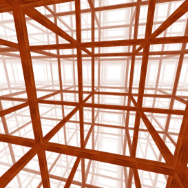
Figure 1: The 3-dimensional cubic kaleidoscopic honeycomb $\{4,3,4\}$. This Figure is courtesy of Roice Nelson [13].

Definition 2.1.

The $k$-skeleton of the canonical cubulation $\mathcal{C}^{n}$ of $\mathbb{R}^{n}$, denoted by $\mathcal{C}^{k}$, consists of the union of the $k$-skeletons of the hypercubes in $\mathcal{C}^{n}$, i.e., the union of all cubes of dimension $k$ contained in the $n$-cubes in $\mathcal{C}^{n}$. We will call the 2-skeleton $\mathcal{C}^{2}$ of $\mathcal{C}^{n}$ the canonical scaffolding of $\mathbb{R}^{n}$.

2.1.2 Hyperbolic cubic honeycombs $\{4,3,5\}$ and $\{4,3,3,5\}$

A gridded surface is a surface made of congruent squares contained in the corresponding scaffoldings which have disjoint interiors and are glued only in their edges, two squares are either disjoint or share one edge or a vertex. Around each vertex there is a circular circuit of squares (the squared star of the vertex). The condition of regularity of platonic solids in the 3-dimensional case implies that the number of squares around each vertex is a constant $k>2$. If $k=3$ then the regular gridded surface is the cube $\{4,3\}$ which is homeomorphic to a sphere $\mathbb{S}^{2}$. If $k=4$ then the regular surface is the gridded plane $\{4,4\}$ which is isometric to the Euclidean plane $\mathbb{R}^{2}$. If $k>4$ then the regular surfaces are the gridded hyperbolic planes which are denoted by $\{4,5\},\{4,6\},...$. These gridded hyperbolic planes are length spaces [2] and are isometric, as length metric spaces to the hyperbolic plane $\mathbb{H}^{2}$.

Analogously, we consider regular gridded 3-manifolds made of congruent cubes in scaffoldings which are disjoint and glued only in their boundary squares, two cubes are either disjoint or meet at a vertex an edge or a square. There is a circular circuit of cubes around each edge and one spherical circuit of cubes around each vertex as PL 3-manifolds. For each edge there is the same number of cubes $k>2$. If $k=3$ then the regular gridded 3-manifold is the hypercube $\{4,3,3\}$ which is homeomorphic to the 3-sphere $\mathbb{S}^{3}$. If $k=4$ then the regular gridded 3-manifold is the cubic space $\{4,3,4\}$ which is isometric to the Euclidean space $\mathbb{R}^{3}$. If $k=5$ then the regular gridded 3-manifold is the cubic hyperbolic 3-space $\{4,3,5\}$ which is isometric as a length space to the hyperbolic 3-space $\mathbb{H}^{3}$ [2].

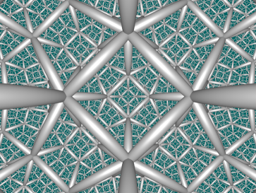
Figure 2: The 3-dimensional cubic hyperbolic honeycomb $\{4,3,5\}$. This Figure is courtesy of Roice Nelson [13].

Finally we construct regular gridded 4-manifolds made of congruent hypercubes contained in the corresponding scaffoldings which are disjoint and glued only in their boundary cubes, two hypercubes are either disjoint, or meet along a boundary cube of some dimension. There is one circular circuit of hypercubes around each square, one 2-spherical circuit of hypercubes around each edge and one 3-spherical circuit of hypercubes around each edge vertex as PL 4-manifolds.

For each square which is a ridge, there is the same number of hypercubes $k>3$. If $k=3$ then the regular gridded 4-manifold is the hypercube $\{4,3,3,3\}$ which is homeomorphic to the 4-sphere $\mathbb{S}^{4}$. If $k=4$ then the regular 4-manifold is the gridded cubic 4-space $\{4,3,3,4\}$ which is isometric to the Euclidean 4-space $\mathbb{R}^{4}$. If $k=5$ then the regular 4-manifold is the gridded hyperbolic 5-space $\{4,3,3,5\}$ which is isometric to the hyperbolic 4-space $\mathbb{H}^{4}$.

The combinatorial structure of the regular hyperbolic honeycomb $\{4,3,5\}$ ($\cal C$) is as follows: there are 12 edges, 30 squares and 20 cubes meeting at every vertex and there are 5 squares and 5 cubes meeting at every edge.

The combinatorial structure of the regular honeycomb $\{4,3,3,5\}$ ($\cal C$) is as follows: there are 120 edges, 720 squares, 1200 cubes and 600 hypercubes meeting at every vertex; there are 6 squares, 32 cubes and 16 hypercubes meeting at every edge and there are 5 cubes and 5 hypercubes meeting at every square.

As before, we define the $k$-skeleton of the hyperbolic honeycomb of $\mathbb{H}^{n}$ ($n=3,4$), denoted by $\mathcal{C}^{k}$, consists of the union of the $k$-skeletons of the hypercubes in $\cal C$, i.e., the union of all cubes of dimension $k$ contained in the $n$-cubes in $\cal C$. We will call the 2-skeleton $\mathcal{C}^{2}$ of $\cal C$ the canonical scaffolding of $\mathbb{H}^{n}$ ($n=3,4$).

2.2 Taxonomy of topological surfaces

Next we will consider all topological surfaces. First we will remind some definitions.

Let $g(S)$ denote the genus of a compact surface $S$. The genus of the noncompact surface $S$ is by definition

$$g(S)=\max\{g(A)\,:\,A\,\,\mbox{is a compact subsurface of}\,\,S\},$$

if this maximum exists, and infinite otherwise ( $g(S)=\infty$).

If $g(S)=0$ we say that the surface $S$ is planar. In this case the surface is homeomorphic to an open subset of the plane.

Definition 2.2.

There are four orientability classes of noncompact surfaces:

1. If every compact subsurface of a surface $S$ is orientable, then $S$ is orientable.

2. If there is no bounded subset $A$ of $S$ such that $S-A$ is orientable, then $S$ is infinitely nonorientable.

3. If $S$ does not belong to (l) or (2) and every sufficiently large subsurface of $S$ contains an even number of cross caps, then $S$ is even non orientable.

4. If $S$ does not belong to (1) or (2) and every sufficiently large subsurface of $S$ contains an odd number of cross caps, then $S$ is odd non orientable.

Definition 2.3.

Let $S$ be a surface. An end of $S$ is a function $e$ which asigns to each compact subset $K$ of $S$ an unbounded, connected component $e(K)$ of $\mbox{Cl}(S-K)$ in such a way that if $K$ and $L$ are compact subsets of $S$ and $K\subset L$ then $e(L)\subset e(K)$. $E_{S}$ denotes the set of all ends of $S$.

If $S$ is a noncompact surface, there is a compact subsurface $A$ of $S$ such that each component of $\mbox{Cl}(S-A)$ is either orientable or infinitely nonorientable, and either planar or of infinite genus. In all that follows $A$ will denote such a subsurface.

Definition 2.4.

Let $e\in E_{S}$. We say that $e$ is nonorientable (or orientable) if $e(A)$ is infinitely nonorientable (or orientable). And $e$ is planar (or of infinite genus) if $e(A)$ is planar (or of infinite genus).

For any surface $S$ consider the nested triple $(E_{S},G_{S},O_{S})$, where $E_{S}$ is the set of ends of $S$, $G_{S}$ is the subset of $E_{S}$ consisting of the ends which are not planar, and $O_{S}$ is the subset of $G_{S}$ of the orientable nonplanar ends.

The next Theorem is by Kerékjárto and Richards, the reader can find it in [14].

Theorem.

(Classification theorem for noncompact surfaces). Let $X$ and $Y$ be two noncompact surfaces of the same genus and orientability class. Then $X$ and $Y$ are homeomorphic if and only if the triads $(E_{X},G_{X},O_{X})$ and $(E_{Y},G_{Y},O_{Y})$ are topologically equivalent.

Remark 2.5.

The condition that $X$ and $Y$ are of the same genus and orientability class guaranties that their bounded parts are homeomorphic. The condition on the subsets of ends makes sure that their asymptotic behavior is the same.

Our goal is to show that any surface is homeomorphic to a gridded surface. In order to prove it, we will use the classification theorem for noncompact surfaces and the theorems of Richards which appear in [14].

Theorem 2.6.

The set of ends of a surface is totally disconnected, separable, and compact. Any compact, separable, totally disconnected space is homeomorphic to a subset of the Cantor set.

Theorem 2.7.

Let $(X,Y,Z)$ be any triple of compact, separable, totally disconnected spaces with $Z\subset Y\subset X$. Then there is a surface S whose ideal boundary $(E_{S},G_{S},O_{S})$ is topologically equivalent to the triple $(X,Y,Z)$.

Theorem 2.8.

Every surface is homeomorphic to a surface formed from a 2-sphere $\mathbb{S}^{2}$ by first removing a closed totally disconnected set $X$ from $\mathbb{S}^{2}$, then removing the interiors of a finite or infinite sequence $D_{1},D_{2},\dots$ of non-overlapping closed discs in $\mathbb{S}^{2}-X$, and finally suitably identifying the boundaries of these discs in pairs, (It may be necessary to identify the boundary of one disc with itself to produce an odd ”cross cap.”) The sequence $D_{1},D_{2},\dots$ ”approaches $X$” in the sense that, for any open set $U\subset\mathbb{S}^{2}$ containing $X$, all but a finite number of the $D_{i}$ are contained in $U$.

Let $X\subset\mathbb{S}^{2}$ a Cantor set, the orientable noncompact surface $\mathbb{S}^{2}-X$ is called the tree of life. The tree of life can be constructed by an infinite set of pair of pants glued along their boundaries. A pair of pants is by definition the surface with boundary $\mathbb{S}^{2}-\{D_{1},D_{2},D_{3}\}$ where each $D_{i}$ is an open disc. Consider the surfaces with boundary $\Sigma_{1}$ and $\Sigma_{2}$ which are the connected sum of a pair of pants with a torus $\Sigma_{1}=\mathbb{T}^{2}-\{D_{1},D_{2},D_{3}\}$ and with a projective plane $\Sigma_{2}=\mathbb{P}^{2}-\{D_{1},D_{2},D_{3}\}$.

A pruned tree of life is obtained from the tree of life removing a set of branches (neighborhoods of ends) cut along boundaries of the corresponding pair of pants where these boundaries are identified to points (i.e, we cap some holes of the pair of pants).

For the purpose of this paper we will rephrase the Theorem 2.8, as follows.

Theorem 2.9.

Every surface is homeomorphic to a surface obtained from a pruned tree of life such that a finite or infinite number of pair of pants are interchanged by either the connected sum of a pair of pants with a torus i.e., $\Sigma_{1}$ or the connected sum of pair of pants with a projective plane i.e., $\Sigma_{2}$.

For instance, consider the plane; i.e. the noncompact surface homeomorhic to $\mathbb{R}^{2}$. Then, it can be obtained from the tree of life if one removes all of its branches except one but and at each boundary component we glue a squared disk. The gridded surface obtained in this way is depicted in Figure 3. In this way, the plane is composed by an infinite number of pair of pants.

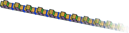
Figure 3: The gridded plane is obtained from the tree of life made of pair of pants after pruning and filling the remaining holes with squares (the left square and the squares at the top).

3 Surfaces in $\{4,3^{n-2},4\}$ in $\mathbb{R}^{n}$

3.1 Compact surfaces in $\{4,3,3,4\}$ in $\mathbb{R}^{4}$

As we mentioned before, we will prove that any connected surface with a finite number of ends is homeomorphic to a gridded surface. We will start considering closed surfaces.

Notice that the 2-sphere $\mathbb{S}^{2}$ and the 2-torus $\mathbb{T}^{2}$ are homeomorphic to gridded surfaces contained in the scaffolding $\mathcal{C}^{2}$ of the canonical cubulation $\cal C$ of $\mathbb{R}^{3}$ in the obvious way. In fact, Consider the unit 3-cube $I^{3}=[0,1]^{3}$, clearly its boundary $\partial I^{3}$ is contained in $\mathcal{C}^{2}$ and is homeomorphic to the 2-sphere $\mathbb{S}^{2}$ (see Figure 4).

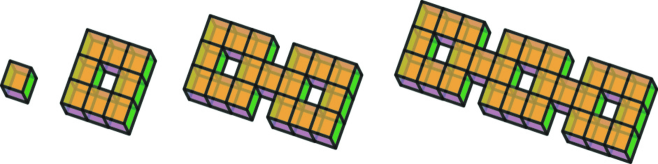
Figure 4: Closed gridded surfaces in $\mathbb{R}^{3}$.

The 2-torus $\mathbb{T}^{2}$ is the gridded surface $S=\cup_{i=0}^{9}F_{i}$ (see the second image of the Figure 4), where $F_{i}$, $i=0,\ldots,9$ are the following 10 sets which are unions of squares (squared sets):

$$F_{0}=\{(x,y,0)\in\mathbb{R}^{3}\,|\,0\leq x,\,y\leq 3\}\setminus\{(x,y,0)\in\mathbb{R}^{3}\,|\,1<x,\,y<2\},$$

$$F_{1}=\{(x,y,1)\in\mathbb{R}^{3}\,|\,0\leq x,\,y\leq 3\}\setminus\{(x,y,0)\in\mathbb{R}^{3}\,|\,1<x,\,y<2\},$$

$$F_{2}=\{(0,y,z)\in\mathbb{R}^{3}\,|\,0\leq y\leq 3,\,\,0\leq z\leq 1\},$$

$$F_{3}=\{(1,y,z)\in\mathbb{R}^{3}\,|\,0\leq y\leq 3,\,\,0\leq z\leq 1\},$$

$$F_{4}=\{(x,0,z)\in\mathbb{R}^{3}\,|\,0\leq x\leq 3,\,\,0\leq z\leq 1\},$$

$$F_{5}=\{(x,1,z)\in\mathbb{R}^{3}\,|\,0\leq x\leq 3,\,\,0\leq z\leq 1\},$$

$$F_{6}=\{(x,1,z)\in\mathbb{R}^{3}\,|\,1\leq x\leq 2,\,\,0\leq z\leq 1\},$$

$$F_{7}=\{(x,2,z)\in\mathbb{R}^{3}\,|\,1\leq x\leq 2,\,\,0\leq z\leq 1\},$$

$$F_{8}=\{(1,y,z)\in\mathbb{R}^{3}\,|\,1\leq y\leq 2,\,\,0\leq z\leq 1\},$$

$$F_{9}=\{(2,y,z)\in\mathbb{R}^{3}\,|\,1\leq y\leq 2,\,\,0\leq z\leq 1\}.$$

Remark 3.1.

Notice that each square $F$ of the canonical cubulation $\cal C$ of $\mathbb{R}^{4}$ (or $\mathbb{R}^{3}$) is determined by its barycenter $B_{F}$. In fact, consider the unitary canonical vectors on $\mathbb{R}^{4}$: $e_{\pm 1}=(\pm 1,0,0,0)$, $e_{\pm 2}=(0,\pm 1,0,0)$, $e_{\pm 3}=(0,0,\pm 1,0)$ and $e_{\pm 4}=(0,0,0,\pm 1)$. Then

$$F=\{ae_{u}+be_{v}\,:\,0\leq a,\,b\leq 1\}+w$$

where $e_{u}$ and $e_{v}$ ($u,v\in\{\pm 1,\,\pm 2,\,\pm 3,\,\pm 4\}$, $|u|\neq|v|$), denote the corresponding unitary canonical vectors and $w$ is a vector with integers in its coordinates, in fact $w$ is a translation vector. Thus $B_{F}=\frac{1}{2}e_{u}+\frac{1}{2}e_{v}+w$.

We identify the squares of the torus with their barycenters, then:

$F_{0}=(\frac{1}{2},\frac{1}{2},0),(\frac{3}{2},\frac{1}{2},0),(\frac{5}{2},\frac{1}{2},0),(\frac{1}{2},\frac{3}{2},0),(\frac{5}{2},\frac{3}{2},0),(\frac{1}{2},\frac{5}{2},0),(\frac{3}{2},\frac{5}{2},0),(\frac{5}{2},\frac{5}{2},0).$

$F_{1}=(\frac{1}{2},\frac{1}{2},1),(\frac{3}{2},\frac{1}{2},1),(\frac{5}{2},\frac{1}{2},1),(\frac{1}{2},\frac{3}{2},1),(\frac{5}{2},\frac{3}{2},1),(\frac{1}{2},\frac{5}{2},1),(\frac{3}{2},\frac{5}{2},1),(\frac{5}{2},\frac{5}{2},1).$

$F_{2}=(0,\frac{1}{2},\frac{1}{2}),(0,\frac{3}{2},\frac{1}{2}),(0,\frac{5}{2},\frac{1}{2}).$

$F_{3}=(1,\frac{3}{2},\frac{1}{2}).$

$F_{4}=(2,\frac{3}{2},\frac{1}{2}).$

$F_{5}=(3,\frac{1}{2},\frac{1}{2}),(3,\frac{3}{2},\frac{1}{2}),(3,\frac{5}{2},\frac{1}{2}).$

$F_{6}=(\frac{1}{2},0,\frac{1}{2}),(\frac{3}{2},0,\frac{1}{2}),(\frac{5}{2},0,\frac{1}{2}).$

$F_{7}=(\frac{3}{2},1,\frac{1}{2}).$

$F_{8}=(\frac{3}{2},2,\frac{1}{2}).$

$F_{9}=(\frac{1}{2},3,\frac{1}{2}),(\frac{3}{2},3,\frac{1}{2}),(\frac{5}{2},3,\frac{1}{2}).$

The Klein bottle and the real projective plane can not be homeomorphic to gridded surfaces contained in the 2-skeleton of $\mathbb{R}^{3}$ (see [17]) but they are homeomorphic to gridded surfaces contained in the 2-skeleton of $\mathbb{R}^{4}$.

Lemma 3.2.

The projective plane $(\mathbb{P}^{2})$ is a gridded surface in $\{4,3,3,4\}$ in $\mathbb{R}^{4}$.

Proof. We construct a gridded version of the crosscap in $\{4,3,3,4\}$ in $\mathbb{R}^{4}$, see Figure 5. In the left we show the projection of the crosscap. In the middle we divide the crosscap in three parts: on the bottom, there is the base which is a cubic box minus two squares, in the middle there is a band and on the top, there is a disk which is the neighborhood of one vertex.

In the top right part of the Figure 5, we can find the description of the combinatorial square complex of the crosscap as a disk consisting on 30 squares, such that points in the circle boundary are identified by the antipodal map. On the bottom, there is a Möbius band contained in this crosscap.

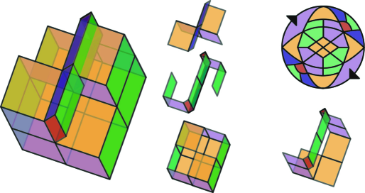
Figure 5: A gridded projective plane in $\mathbb{R}^{4}$. The first figure at the left is the projection of the crosscap into $\mathbb{R}^{3}$.

The gridded crosscap is formed by 30 squares in planes parallel to five of the six coordinate planes in $\mathbb{R}^{4}$ and whose barycenters are:

$XY$: $(\frac{1}{2},\frac{1}{2},0,0),$ $(\frac{3}{2},\frac{1}{2},0,0),$ $(\frac{3}{2},\frac{3}{2},0,0),$ $(\frac{1}{2},\frac{3}{2},0,0),$ $(\frac{3}{2},\frac{1}{2},1,0),$ $(\frac{1}{2},\frac{3}{2},1,0),$ $(\frac{1}{2},\frac{1}{2},2,0),$ $(\frac{3}{2},\frac{3}{2},2,0).$

$XZ$: $(\frac{1}{2},0,\frac{1}{2},0),$ $(\frac{1}{2},0,\frac{3}{2},0),$ $(\frac{3}{2},0,\frac{1}{2},0),$ $(\frac{1}{2},1,\frac{3}{2},0),$ $(\frac{3}{2},1,\frac{3}{2},0),$ $(\frac{1}{2},2,\frac{1}{2},0),$ $(\frac{3}{2},2,\frac{1}{2},0),$ $(\frac{3}{2},2,\frac{3}{2},0).$

$YZ$: $(0,\frac{1}{2},\frac{1}{2},0),$ $(0,\frac{1}{2},\frac{3}{2},0),$ $(0,\frac{3}{2},\frac{1}{2},0),$ $(1,\frac{1}{2},\frac{3}{2},1),$ $(1,\frac{3}{2},\frac{3}{2},1),$ $(2,\frac{1}{2},\frac{1}{2},0),$ $(2,\frac{3}{2},\frac{1}{2},0),$ $(2,\frac{3}{2},\frac{3}{2},0).$

$YW$: $(1,\frac{1}{2},1,\frac{1}{2}),$ $(1,\frac{1}{2},2,\frac{1}{2}),$ $(1,\frac{3}{2},1,\frac{1}{2}),$ $(1,\frac{3}{2},2,\frac{1}{2}).$

$ZW$: $(1,0,\frac{3}{2},\frac{1}{2}),$ $(1,2,\frac{3}{2},\frac{1}{2}).$

These are explictely the 30 squares in $\mathbb{R}^{4}$ corresponding to the disk at the top right of figure 5 (after identifying diametrically opposite points).

Remark 3.3.

If $S$ is a gridded surface contained in the scaffolding $\mathcal{C}^{2}$ of the canonical cubulation $\cal C$ of $\mathbb{R}^{3}$, then $S$ is a gridded surface contained in the scaffolding $\mathcal{C}^{2}$ of the canonical cubulation $\cal C$ of $\mathbb{R}^{4}$, since $\mathbb{R}^{3}$ is canonically isomorphic to the hyperplane ${\cal{P}}=\mathbb{R}^{3}\times\{0\}\subset\mathbb{R}^{4}$ and ${\cal{P}}$ has a canonical cubulation ${\cal{C}}_{\cal{P}}$ given by the restriction of the cubulation $\cal C$ of $\mathbb{R}^{4}$ to it; i.e., ${\cal{C}}_{\cal{P}}$ is the decomposition into cubes which are the images of the unit cube $I^{3}=\{(x_{1},x_{2},x_{3},0)\,|\,0\leq x_{i}\leq 1\}$ by translations by vectors with integer coefficients whose last coordinate is zero.

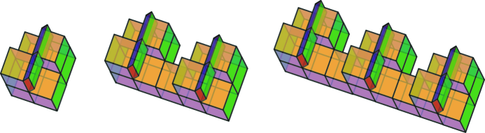
Figure 6: Closed gridded non-orientable surfaces in $\mathbb{R}^{4}$ (the first figure is the projection of the crosscap in $\mathbb{R}^{3}$ following the description of figure 5).

Let $S_{1}$ and $S_{2}$ be two gridded surfaces. In a natural way, we define the gridded connected sum $\#_{g}$ of $S_{1}$ and $S_{2}$, denoted by $S_{1}\#_{g}S_{2}$, as follows: We choose embeddings $i_{j}:\mathbb{D}^{2}\rightarrow S_{j}$ $(j=1,2)$, such that $i_{j}(\mathbb{D}^{2})$ is a unit square $F_{i}$ into $S_{i}$, $i=1,2$. We can assume, up to applying rigid movements that $F_{1}$ and $F_{2}$ are faces of some 3-cube $Q$ which its interior does not intersect neither $S_{1}$ or $S_{2}$. Thus we obtain $S_{1}\#_{g}S_{2}$ from the disjoint sum $(S_{1}\setminus\operatorname{Int}(Q_{1}))\sqcup(S_{2}\setminus\operatorname{Int}(Q_{2}))$ joining $F_{1}$ with $F_{2}$ via the four remaining faces of $Q$ (see Figure 7). Observe that $S_{1}\#_{g}S_{2}$ is homeomorphic to the usual connected sum $S_{1}\#S_{2}$.

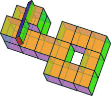
Figure 7: The gridded connected sum of gridded surfaces is gridded.

Lemma 3.4.

If $S_{1}$ and $S_{2}$ are surfaces homeomorphic to gridded surfaces $C_{1}$ and $C_{2}$, respectively; then the connected sum $S_{1}\#S_{2}$ is homeomorphic to the gridded connected sum $C_{1}\#_{g}C_{2}$.

Proof. Consider the gridded surfaces $C_{1}$ and $C_{2}$. Then $C_{1}\#_{g}C_{2}$ is homeomorphic to $C_{1}\#C_{2}$. Therefore $C_{1}\#_{g}C_{2}$ is homeomorphic to $S_{1}\#S_{2}$. $\square$

Summarizing, from the above Lemmas and using the classification theorem for closed surfaces, we have the following.

Theorem 3.5.

Any closed surface $S$ is homeomorphic to a gridded surface $C$ such that if $S$ is orientable then $C$ is contained in the scaffolding $\mathcal{C}^{2}$ of the canonical cubulation $\cal C$ of $\mathbb{R}^{3}$, and if $S$ is non orientable then $C$ is contained in the scaffolding $\mathcal{C}^{2}$ of the canonical cubulation $\cal C$ of $\mathbb{R}^{4}$.

3.2 Gridded surfaces in $\{4,3,4\}$ and $\{4,3,3,4\}$ in $\mathbb{R}^{3}$ and $\mathbb{R}^{4}$

We will show that all connected surfaces (orientable or not) can be gridded in $\mathbb{R}^{4}$ and moreover all orientable connected surfaces can be gridded in $\mathbb{R}^{3}$.

This follows from the fact that the 3-regular infinite tree graph can be embedded in the 1-skeleton of the 4-regular tessellation of squares in the Euclidean plane (canonical cubulation of $\mathbb{R}^{2}$). Then we thicken this tree graph to get a gridded tree of life in $\mathbb{R}^{3}$ or $\mathbb{R}^{4}$. In order to obtain a connected surface from our gridded tree of life, we glue a set of tori and/or projective planes to the pruned tree of life corresponding to the given surface.

Lemma 3.6.

The 3-regular infinite tree graph (i.e., a connected infinite regular tree of degree 3) can be embedded in the 1-skeleton of the 4-regular tessellation of squares in the Euclidean plane (canonical cubulation of $\mathbb{R}^{2}$).

Proof.

We will construct a 3-regular infinite tree graph embedded in the 1-skeleton of the 4-regular tessellation of squares in the Euclidean plane $\mathbb{R}^{2}$ as a spiral. The trivalent vertices are the elements of the set $\{(n,2n)|n\in\mathbb{N}\}$ (see left part of Figure 8). More precisely, we start from the origin $O=(0,0)$, and we consider the following two paths: one from $O$ to $(0,1)$ and the other one from $O$ to $(1,0)$ and then from $(1,0)$ to $(1,3)$. Next we set two paths $\gamma^{n}_{1}$ and $\gamma^{n}_{2}$ at each vertex $(n,2n+1)$, $n\in\mathbb{N}$. Notice that each path in the 1-skeleton of our cubulation of $\mathbb{R}^{2}$ can be described in a unique way by a sequence of adjacent vertices on the $\mathbb{Z}^{2}$-lattice which is described by arrows. Using the above, we have that

$${\scriptstyle\gamma^{n}_{1}=[(n,2n+1)\to(-2n-1,2n+1)\to(-2n-1,-2n-1)\to(2n+2,-2n-1)\to(2n+2,4n+5)]}$$

and

$${\scriptstyle\gamma^{n}_{2}=[(n,2n+1)\to(n,2n+2)\to(-2n-2,2n+2)\to(-2n-2,-2n-2)\to(2n+3,-2n-2)to(2n+3,4n+7)].}$$

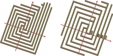
Figure 8: Left: The tree of life gridded in $\mathbb{R}^{3}$. Right: A general noncompact surface gridded in $\mathbb{R}^{4}$.

The infinite union of paths is our desired 3-regular infinite tree graph. $\square$

Theorem 3.7.

Any connected surface $S$ is homeomorphic to a gridded surface $C$ such that if $S$ is orientable then $C$ is contained in the scaffolding $\mathcal{C}^{2}$ of the canonical cubulation $\cal C$ of $\mathbb{R}^{3}$, and if $S$ is non orientable then $C$ is contained in the scaffolding $\mathcal{C}^{2}$ of the canonical cubulation $\cal C$ of $\mathbb{R}^{4}$.

Proof.

Given a connected surface $S$, we will construct a homeomorphic gridded copy of it by means of Richard’s Theorem. First, we recall that $S$ can be obtained from the tree of life by removing a set of branches to get the corresponding pruned tree of life $P$ and next, we interchanged a finite or infinite number of pair of pants of $P$ by either the connected sum of a pair of pants with a torus or the connected sum of a pair of pants with a projective plane to get $S$ (see Theorem 2.9).

Let $T$ be the infinite regular tree graph of degree 3. Then by the previous Lemma, $T$ can be embedded in the 1-skeleton of the 4-regular tessellation by squares in the Euclidean plane $\mathbb{R}^{2}$. Now, we apply the homothetic transformation $x\mapsto 5x$ in $\mathbb{R}^{2}$ to expand $T$ obtaining a new tree graph $\hat{T}$ whose edge size is now 5 units. Notice that the plane $\mathbb{R}^{2}$ is embedded in a natural way into $\mathbb{R}^{3}$ as the set of points whose third coordinate is zero. Let $V$ be the union of all cubes that intersect $\hat{T}$, so its boundary $\mathfrak{T}$ is a surface homeomorphic to the tree of life embedded in the 2-skeleton of the canonical cubulation of $\mathbb{R}^{3}$ (see Figure 8). By Richard’s Theorem, we obtain $S$ gluing a set of tori and/or projective planes to the pruned tree of life corresponding to $S$. Notice that the space of ends $E_{\mathfrak{T}}$ of the tree of life $\mathfrak{T}$ is homeomorphic to the Cantor set, $C$, and our surface $S$ is determined by a nested sequence of three closed subsets of the Cantor set $(E_{S},G_{S},O_{S})$ where $O_{S}\subset{G_{S}}\subset{E_{S}}$.

Let $\phi:E_{\mathfrak{T}}\rightarrow C$ be a homeomorphism of the set of ends of our tree of life into the Cantor set, and consider a homeomorphism $\Psi:E_{S}\to E^{\prime}\subset{E_{\mathfrak{T}}}$ of the sets of ends of $S$ into the set of ends of our tree of life. The ends that do not belong to $\Psi(E_{S})$ are pruned and closed by squares to obtain a surface without boundary. Observe that the pair of pants of the tree of life are in correspondence with the vertices $(0,n),n\in\mathbb{N}$, hence we glue tori and projective planes into pair of paints around these vertices $(0,n)$ and according to the images of $(E_{S},G_{S},O_{S})$ into $E_{\mathfrak{T}}$. First glue tori on the respective pair of paints of the orientable non planar ends $O_{S}$ an next glue projective planes on the respective pair of paints of the ends in $G_{S}-O_{S}$ (see right part of Figure 8).

If the surface $S$ is non orientable but $G_{S}-O_{S}=$ the there are two cases: If $O_{S}\neq$ only is necessary glue one or two projective planes if $S$ is non orientable non or even, respectively. If $O_{S}=$ then its necessary glue a finite number of projective planes and/or tori.

Notice that they are disjoint since the diameter of such pieces is less than the distance of the pair of parts of our surface. Therefore, $S$ is gridded in $\mathbb{R}^{4}$ or $\mathbb{R}^{3}$ if $S$ is orientable. $\square$

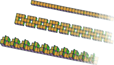
Figure 9: Types of ends of a surface with finite ends. A cylinder, an infinite ladder and an infinite chain of crosscaps.

Remark 3.8.

If the surface to considerer has a finite number of ends the we can consider a closed gridded surface and glue the ends which are of three types: the cilinder, the infinite ladder (an infinite chain of tori) and an infinite chain of projective planes. See Figure 9.

4 Orientable surfaces in $\{4,3,5\}$ in $\mathbb{H}^{3}$

All orientable surfaces can be constructed as gridded surfaces on the hyperbolic cubic honeycomb $\{4,3,5\}$ of the hyperbolic space $\mathbb{H}^{3}$. We proceed as in the Euclidean case where we proof that the orientable closed surfaces are gridded in $\mathbb{R}^{3}$ by means gridded the torus and the connected sum of two gridded surfaces.

Lemma 4.1.

The torus is a gridded surface in $\{4,3,5\}$ in $\mathbb{H}^{3}$. Moreover, all closed orientable surfaces are gridded surfaces in $\{4,3,5\}$ in $\mathbb{H}^{3}$.

Proof.

Let the torus be the gridded surface obtained as the boundary of twelve consecutive cubes in $\{4,3,5\}$ whose union looks like as O. There are a central removed cube and there are 4 cubes around each of its four hyperparallel edges (see Figure 10). This gridded torus in hyperbolic space is the one with the minimum number of squares in the scaffolding of $\{4,3,5\}$. It has 44 squares.

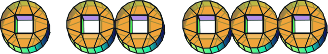
Figure 10: Torus and closed orientable surfaces in $\{4,3,5\}$ in $\mathbb{H}^{3}$.

There is a completely analogous hyperbolic concept of connected sum for gridded surfaces as in the previous Euclidean section. Let $S_{1}$ and $S_{2}$ gridded surfaces in $\mathbb{H}^{3}$ and $D_{1}\subset S_{1}$ and $D_{2}\subset S_{2}$ two squares such that each one of the corresponding support hyperbolic plane $\hat{D_{i}}$ $i=1,2$, divides $\mathbb{H}^{3}$ in two half–spaces in such a way that $S_{i}$ is contained in only one half–space. Then we can construct the connected sum $S_{1}\#S_{2}$ as a gridded surface. A closed orientable surface can be gridded in this hyperbolic context as a connected sum of gridded tori. ∎

A hyperbolic pair of pants is a closed pair of pants with a hyperbolic metric such that each of its three boundary circles are geodesics. The isometry class of such pair of pants is determined by the triple of lengths $(l_{1},l_{2},l_{3})$ of the boundaries.

Lemma 4.2.

The pair of pants is a gridded surface in $\{4,3,5\}$ in $\mathbb{H}^{3}$.

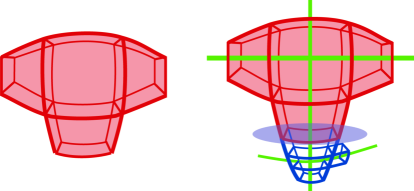
Figure 11: A gridded pair of pants in $\{4,3,5\}$ in $\mathbb{H}^{3}$.

Proof.

Let the pair of pants be the gridded surface obtained as the boundary of four cubes in $\{4,3,5\}$ whose union looks like as T minus three squares. There are a central cube $C$ and three neighborhood cubes $C_{i}$ of it such that these four cubes do not share a vertex; i.e. $C\cap\cup_{i=1}^{3}C_{i}=\emptyset$. Then $C\#C_{1}\#C_{2}\#C_{3}$ is our pair of pants (see Figure 11). ∎

Lemma 4.3.

The tree of life is a gridded surface in $\{4,3,5\}$ in $\mathbb{H}^{3}$.

Proof.

The proof is constructive by means pair of pants pasted along their boundaries as an infinite tree.

There are two distinguished geodesics in our model of the pair of pants. Notice that a pair of pants has a rotational symmetry of order 2. The axis of symmetry is a geodesic which pass through the barycenters of the central cube and the second neighborhood cube i.e. the vertical bar in the T. The second axis is the geodesic perpendicular to the axis of symmetry which passes through the barycenters of the central cube and the first and third neighborhood cubes i.e. the horizontal bar in the T. The axis of symmetry is ultraparallel to the two squares which were removed from the first and third neighborhood cubes and the second axis is ultraparallel to the square which was removed from the second neighborhood cube.

Then we can construct inductively the tree of life. We start by a pair of pants $P$ and glue it both a square in the boundary of the second cube and two pairs of pants $P_{i}$ at each boundary of the first and third cubes of $P$ with the second neighborhood cubes of the corresponding $P_{i}$; in such away that all barycenters of the cubes are lie in one hyperbolic plane (see Figure 11). The second axis of the first pair of pants is the axis of symmetry of the two pair of pants which have been glued to its first and third neighborhood cubes. The second axis of the new two cubes is ultraparallel to the axis of symmetry of the original cube and these geodesics are ultraparallel to the hyperbolic plane defined by the square of gluing of each two pair of pants. This plane divides the tree of life in two connected components.

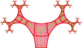
Figure 12: Gridded Tree of life in $\{4,3,5\}$ in $\mathbb{H}^{3}$.

We glue new pairs of pants by the second neighborhood cube in the boundaries of the surface such that all barycenters of the cubes are in the hyperbolic plane. The step of induction is that the second axis of the pair of pants in the surface is the axis of symmetry of the two pair of pants which have been glued to their first and third neighborhood cubes. The second axis of the new two cubes is ultraparallel to the axis of symmetry of the original cube and these geodesics are ultraparallel to the hyperbolic plane defined by the square of gluing of each two pair of pants. This plane divides the tree of life in two connected components. By induction, we have constructed the tree of life. ∎

We are ready to prove the following theorem.

Theorem 4.4.

Any connected orientable surface is homeomorphic to a gridded surface in $\{4,3,5\}$ in $\mathbb{H}^{3}$.

Proof. Any connected orientable surface can be constructed from the pruned tree of life replacing some pair of pants by “handles”. We can consider the gridded torus minus three nonconsecutive equatorial squares. Notice that when we exchange a pair of pants by these gridded tori minus three nonconsecutive equatorial squares, the property of the gridded connected sum is preserved. The hyperbolic planes which pass through the boundaries of the modified pair of pants are ultraparallels, then the construction of a tree of life with handles is analogous to the planar tree of life.

5 Surfaces in $\{4,3,3,5\}$ in $\mathbb{H}^{4}$

One great difference between the Euclidean and the hyperbolic gridded cases is that the gridded Euclidean spaces are nested and the gridded hyperbolic spaces are not (as gridded spaces). For the Euclidean case we proof that the orientable closed surfaces are gridded in $\mathbb{R}^{3}$ by means gridded the torus and the connected sum. We proved that the projective plane is gridded in $\mathbb{R}^{4}$ and all closed surfaces are gridded in $\mathbb{R}^{4}$.

The gridded hyperbolic 3-space $\{4,3,5\}$ is not contained in the gridded hyperbolic 4-space $\{4,3,3,5\}$. However, it is not a great problem to grid in $\mathbb{H}^{4}$ all the gridded surfaces in $\mathbb{H}^{3}$. We need to grid the torus, the pair of pants and the connected sum of gridded surfaces in order to obtain all orientable surfaces. For nonorientable surfaces we need only to prove that the projective plane is gridded in $\mathbb{H}^{4}$ and applying the Richards Theorem then we will obtain all surfaces gridded in $\mathbb{H}^{4}$.

Lemma 5.1.

The torus is a gridded surface in $\{4,3,3,5\}$ in $\mathbb{H}^{4}$. Moreover, all closed orientable surfaces are gridded surfaces in $\{4,3,3,5\}$ in $\mathbb{H}^{4}$.

Proof.

There are 8 cubes in the hypercube forming two linked tori in $\mathbb{S}^{3}$ (see Figure 13). We take one of these torus. Let the torus be the gridded surface obtained as the boundary of four consecutive cubes in a hypercube $\{4,3,3\}$.

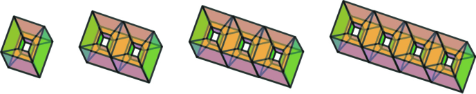
Figure 13: Gridded torus and closed orientable surfaces in $\{4,3,3,5\}$ in $\mathbb{H}^{4}$.

As above, we have a 4-dimensional analogous hyperbolic concept of connected sum for gridded surfaces. Let $S_{1}$ and $S_{2}$ be two hyperbolic gridded surfaces $\mathbb{H}^{4}$ and $D_{i}\subset S_{i}$, $i=1,2$ be squares such that the corresponding support hyperbolic plane $\hat{D_{i}}$ lies in a 3-dimensional geodesic hyperbolic subspace which divides $\mathbb{H}^{4}$ in two half–spaces such that $S_{i}$ is contained in only one half–space. Then we can construct the connected sum $S_{1}\#S_{2}$ as a gridded surface. A closed orientable surface can be gridded in this hyperbolic context as a connected sum of gridded tori. ∎

Lemma 5.2.

The pair of pants is a gridded surface in $\{4,3,3,5\}$ in $\mathbb{H}^{4}$.

Proof.

Consider three 3-faces $F_{1}$, $F_{2}$ and $F_{3}$ of three consecutive hypercubes $C_{1}$, $C_{2}$ and $C_{3}$ such that $F_{i}\subset C_{i}$ ($i=1,2,3$) and $F_{1}\cap F_{2}$ and $F_{2}\cap F_{3}$ are two disjoint squares. The barycenters of $C_{1}$, $C_{2}$ and $C_{3}$ are collinear. Consider the connected sum $F_{1}\#F_{2}\#F_{3}$. Notice that $F_{1}\#F_{2}\#F_{3}$ is homeomorphic to a $\mathbb{S}^{2}$. Then the pair of pants is obtained from $F_{1}\#F_{2}\#F_{3}$ by removing one boundary square $S_{i}$ from $F_{i}$, in such a way that $S_{1}$ is parallel to $F_{1}\cap F_{2}$ and $S_{3}$ is parallel to $F_{2}\cap F_{3}$ (see Figure 14). ∎

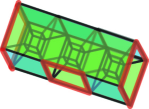
Figure 14: The gridded pair of pants in $\{4,3,3,5\}$ in $\mathbb{H}^{4}$.

Lemma 5.3.

The tree of life is a gridded surface in $\{4,3,3,5\}$ in $\mathbb{H}^{4}$.

Proof.

The proof is constructive using pair of pants pasted along their boundaries as an infinite tree.

There are two important geodesics in our model of a pair of pants. A pair of pants has a rotational symmetry of order 2. The axis of symmetry is a geodesic which passes through the barycenter of $F_{2}$ and the barycenter of the square $S_{2}$. The second axis is the geodesic perpendicular to the axis of symmetry which passes through the barycenters of $S_{1}$ and $S_{3}$. The axis of symmetry is ultraparallel to the two squares which were removed from $F_{1}$ and $F_{3}$ and the second axis is ultraparallel to the square which was removed from $F_{2}$.

We can construct inductively the tree of life in analogous way as $\mathbb{H}^{3}$. ∎

Lemma 5.4.

The projective plane is a gridded surface in $\{4,3,3,5\}$ in $\mathbb{H}^{4}$.

Proof. We construct a gridded version of the crosscap in $\{4,3,3,5\}$ in $\mathbb{H}^{4}$. See the Figures 5 and 15. In the left we show the projection of the crosscap. In the middle we divide the crosscap in three parts: at the bottom, there is the base which is a pentagonal cubic box minus two squares at the top. In the middle, there is a band and at the top there is a disk which is a neighborhood of one vertex. Only the base is different in the two Figures 5 and 15.

In the right part of the Figure 15 there is a description of the combinatorial square complex of the crosscap as a disk with 34 squares after identifying points in the circle boundary by the antipodal map. At the bottom, there is a Möbius band contained in this crosscap. This is similar to the Euclidean case except one uses 4 more squares in the crosscap (see figure 5).

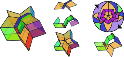
Figure 15: Gridded projective plane in $\{4,3,3,5\}$ in $\mathbb{H}^{4}$.

We are ready to prove the following theorem.

Theorem 5.5.

Any connected surface is homeomorphic to a gridded surface in $\{4,3,3,5\}$ in $\mathbb{H}^{4}$.

Proof. Any connected surface can be constructed from the pruned tree of life modifying some pair of pants by means put “handles” and “projective planes”. Consider the connected sum of a hyperbolic gridded torus in $\{4,3,3,5\}$ and the pair of pants. In fact, from a gridded torus we remove an open square and we paste the boundary of this square onto the boundary of a removed square in the central cube $F_{2}$ of the pair of pants (see Figure 16).

Figure 16: Tree of life with handles and projective planes. The non-planar non orientable ends go to the top left and the orientable non-planar ends go to the top right.

As above, we consider the connected sum of a hyperbolic gridded projective plane in $\{4,3,3,5\}$ and the pair of pants. Remove from the gridded projective plane an open square in its base and paste its boundary with the boundary of one square in the central cube $F_{2}$ of the pair of pants.

Notice that, if we exchange a pair of pants of a pruned tree of life by these kind of new pair of pants the property of the gridded connected sum is preserved. The hyperbolic spaces which pass by the boundaries of these new pair of pants are ultraparallels and divide $\mathbb{H}^{4}$ in two half–spaces where the pair of pants is contained in one component. Then the construction of a tree of life with handles and projective planes is analogous to the construction of an orientable noncompact surface in $\mathbb{H}^{3}$ (see Theorem 4.4).

J. P. Díaz. Instituto de Matemáticas, Unidad Cuernavaca. Universidad Nacional Autónoma de México. Av. Universidad s/n, Col. Lomas de Chamilpa. Cuernavaca, Morelos, México, 62209.

E-mail address: juanpablo@matcuer.unam.mx

G. Hinojosa. Centro de Investigación en Ciencias. Instituto de Investigación en Ciencias Básicas y Aplicadas. Universidad Autónoma del Estado de Morelos. Av. Universidad 1001, Col. Chamilpa. Cuernavaca, Morelos, México, 62209.

E-mail address: gabriela@uaem.mx

A. Verjovsky. Instituto de Matemáticas, Unidad Cuernavaca. Universidad Nacional Autónoma de México. Av. Universidad s/n, Col. Lomas de Chamilpa. Cuernavaca, Morelos, México, 62209.

E-mail address: alberto@matcuer.unam.mx

References

- [1] M. Boege, G. Hinojosa, and A. Verjovsky. Any smooth knot is isotopic to a cubic knot contained in the canonical scaffolding of . Rev. Mat Complutense (2011) 24: 1–13. DOI 10.1007/s13163-010-0037-4.
- [2] M. Burago, Y. Burago, S. Ivanov. A course in metric geometry. Graduate Studies in Mathematics, 33. American Mathematical Society, Providence, RI, 2001. xiv+415 pp. ISBN: 0-8218-2129-6
- [3] Yuanan Diao. Minimal Knotted Polygons on the Cubic Lattice. Journal of Knot Theory and Its Ramifications, vol. 2, no. 4 (1993) 413–425.
- [4] N. P. Dolbilin, M. A. Shtan ko, M. I. Shtogrin. Cubic manifolds in lattices. Izv. Ross. Akad. Nauk Ser. Mat. 58 (1994), no. 2, 93-107; translation in Russian Acad. Sci. Izv. Math. 44 (1995), no. 2, 301-313.
- [5] N. V. Efimov. Impossibility of a complete regular surface in Euclidean 3-Space whose Gaussian curvature has a negative upper bound. Doklady Akad. Nauk. SSSR 150 (1963), 1206–1209 (Russian); Engl. transl. in Sov. Math. (Doklady) 4 (1963), 843–846.
- [6] R. H. Fox. A Quick Trip Through Knot Theory. Topology of 3-Manifolds and Related Topics. Prentice-Hall, Inc., 1962.
- [7] L. Funar. Cubulations, immersions, mappability and a problem of Habegger. Ann. scient. Éc. Norm. Sup., 4e série, t. 32, 1999, pp. 681–700.
- [8] M. Gromov. Partial Differential Relations. Ergebnisse der Mathematik und ihrer Grenzgebiete; 3. Folge, Bd. 9, Springer, Berlin, 1986.
- [9] D. Hilbert, Über Flächen von constanter Gauscher Krümmung. Trans. Amer. Math. Soc. 2 (1901), 87–99.
- [10] G. Hinojosa, A. Verjovsky, C. Verjovsky Marcotte. Cubulated moves and discrete knots. Journal of knot theory and its ramifications, Vol 22, No. 14 (2013) 1350079 (26 pages). DOI: 10.1142/S021821651350079X
- [11] B. Mazur. The definition of equivalence of combinatorial imbeddings. Publications mathématiques de l’I.H.É.S., tome 3 (1959) p.5–17.
- [12] S. Matveev, M. Polyak. Finite-Type Invariants of Cubic Complexes. Acta Applicandae Mathematicae 75, pp. 125–132, 2003.
- [13] https://plus.google.com/+RoiceNelson/posts
- [14] I. Richards. On the Classification of Noncompact Surfaces. Trans. Amer. Math. Soc. 106 (1963), 259-269.
- [15] Vladimir A. Rokhlin, New results in the theory of four-dimensional manifolds. Doklady Acad. Nauk. SSSR (N.S.) 84 (1952) 221–224.
- [16] D. Rolfsen. Knots and Links. Publish or Perish, Inc. 1976.
- [17] H. Samelson, Orientability of Hypersurfaces in . Proceedings of the American Mathematical Society, Vol. 22, No. 1 (Jul., 1969), pp. 301–302.
- [18] D. Struik. A Concise History of Mathematics. 3rd. ed., Dover, New York, 1967.
- [19] Živaljević, Rade T. Combinatorial groupoids, cubical complexes, and the Lovász conjecture. Discrete Comput. Geom. 41 (2009), no. 1, 135–161.