Black-Box Optimization in Machine Learning
with Trust Region Based Derivative Free Algorithm

Abstract

In this work, we utilize a Trust Region based Derivative Free Optimization (DFO-TR) method to directly maximize the Area Under Receiver Operating Characteristic Curve (AUC), which is a nonsmooth, noisy function. We show that AUC is a smooth function, in expectation, if the distributions of the positive and negative data points obey a jointly normal distribution. The practical performance of this algorithm is compared to three prominent Bayesian optimization methods and random search. The presented numerical results show that DFO-TR surpasses Bayesian optimization and random search on various black-box optimization problem, such as maximizing AUC and hyperparameter tuning.

1 Introduction

Most machine learning (ML) models rely on optimization tools to perform training. Typically these models are formed so that at least stochastic estimates of the gradient can be computed; for example, when optimizing least squares or logistic loss of a neural network on a given data set. Lately, however, with the increasing need to tune hyperparameters of ML models, black-box optimization methods have been given significant consideration. These methods do not rely on any explicit gradient computation, but assume that only function values can be computed, usually with noise.

There are two relatively independent directions of research for black-box optimization–Bayesian Optimization (BO) (Mockus, 1994; Brochu et al., 2010), predominantly popular in the ML community, and derivative free optimization (DFO) (Conn et al., 2009)–popular in the optimization community. There are other classes of methods for black-box optimization developed in the fields of simulation optimization and engineering, but they are more specialized and we will not focus on them here.

Both BO and DFO methods are usually applied to functions that are not known to be convex. The key difference between the BO and DFO methods, is that BO methods always contain a component that aims at the exploration of the space, hence seeking a global solution, while DFO methods are content with a local optimum. However, it has been shown in DFO literature (More & Wild, 2009) that DFO methods tend to escape shallow local minima and are quite well suited for problems with a few well defined local basins (and possibly many small local basins that appear due to noise).

BO until recently have been established as the method of choice for hyperparameter optimization (HPO). While BO methods have been shown to be effective at finding good solutions (not always globally optimal, as that can only be achieved in the limit), their efficiency slows down significantly as the number of iterations grows. Overall, the methods are quite computationally costly and scale poorly with the number of hyperparameters. Recently, the BO efficiency has been called into question in comparison with a simple random search (Li et al., 2016), whose iterations require nothing, but function evaluations. Moreover, some improvements on random search have been proposed to incorporate cheeper function evaluations and further increase its efficiency for HPO.

In this paper, we will explore properties of an efficient class of DFO methods–model-based trust region methods–in application to problems in ML. We will show that these methods can be more efficient than BO and random search, especially for problems of dimensions higher than 2 or 3. In the specific case of HPO, hyperparameters can be continuous, discrete or categorical. While some DFO methods have been developed for the case of optimization over categorical or binary variables, these methods essentially rely on local search heuristics and we do not consider them here. Our goal is to examine, in detail, the behavior of various black-box methods in a purely continuous setting. We also aim to explore practical scalability of the methods with respect to the dimension of the search space and nonlinearity of the function. While we will list some experiments on HPO problems, these problems are limited to three continuous hyperparameters. Hence, to perform our comparison on problems of larger dimension, we mainly focus on a different problem–optimizing Area Under Receiver Operating Characteristic (ROC) Curve (AUC) (Hanley & McNeil, 1982), over a set of linear classifiers.

AUC is a widely used measure for learning with imbalanced data sets, which are dominant in ML applications. Various results has been reported in terms of comparing the AUC value as a performance measure of a classifier versus the usual prediction accuracy, that is the total percentage of misclassified examples (Bradley, 1997; Ferri et al., 2002; Brefeld & Scheffer, 2005; Lu et al., 2010). In particular, in (Bradley, 1997), AUC is used to evaluate the performance of some ML algorithms such as decision trees, neural networks, and some statistical methods, where, experimentally, it is shown that AUC has advantages over the accuracy. In (Cortes & Mohri, 2004), a statistical analysis of the relationship between AUC and the error rate, including the expected value and the variance of AUC for a fixed error rate, has been presented. Their results show that the average AUC value monotonically increases with the classification accuracy, but in the case of uneven class distributions, the variance of AUC can be large. This observation implies that the classifiers with the same fixed low accuracy may have noticeably different AUC values. Therefore, optimizing AUC value directly may be desirable, however doing so using gradient-based optimization techniques is not feasible, because this function is a discontinuous step function, hence its gradients are either zero or undefined.

This difficulty motivates various state-of-the-art techniques optimizing an approximation of this discontinuous loss function. In (Yan et al., 2003; Herschtal & Raskutti, 2004; Calders & Jaroszewicz, 2007), various smooth nonconvex approximation of AUC has been optimized by the gradient descent method. Alternatively, a ranking loss, which is defined as $1-$AUC value, is minimized approximately, by replacing it with the pairwise margin loss, such as exponential loss, logistic loss, and hinge loss (Joachims, 2006; Steck, 2007; Rudin & Schapire, 2009; Zhao et al., 2011), which results in a convex problem. In terms of computational effort, each iteration of the gradient descent algorithm applied to the pairwise exponential or logistic loss has quadratic computational complexity with the number of training samples $N$. However, computing the gradient of the pairwise hinge loss can be done by a method with the reduced complexity of $\mathcal{O}(N\log N)$. The same method can be applied to compute the AUC value itself, which we utilize in our approach.

In this work, we apply a variant of a model-based trust region derivative free method, called DFO-TR, (Conn et al., 2009) to directly maximize the AUC function over a set of linear classifiers, without using any hyperparameters. We note that in HPO the black-box function is often the validation error or accuracy achieved by the classifier trained using some given set of hyperparameters. Hence, like AUC this function is often piecewise constant and discontinuous. Thus, we believe that optimizing AUC directly and HPO in continuous domains have many common properties as black-box optimization problems. The main goal of this work is to demonstrate the advantages of the DFO-TR framework over other black-box optimization algorithms, such as Bayesian optimization and random search for various ML applications.

Bayesian optimization is known in the ML community as a powerful tool for optimizing nonconvex objective functions, which are expensive to evaluate, and whose derivatives are not accessible. In terms of required number of objective function evaluations, Bayesian optimization methods are considered to be some of the most efficient techniques (Mockus, 1994; Jones et al., 1998; Brochu et al., 2010) for black-box problems of low effective dimensionality. In theory, Bayesian optimization methods seek global optimal solution, due to their sampling schemes, which trade-off between exploitation and exploration (Brochu et al., 2010; Eggensperger et al., 2013). Specifically, Bayesian optimization methods construct a probabilistic model by using point evaluations of the true function. Then, by using this model, the subsequent configurations of the parameters will be selected (Brochu et al., 2010) by optimizing an acquisition function derived from the model. The model is built based on all past evaluation points in an attempt to approximate the true function globally. As a result, the acquisition function is often not trivial to maintain and optimize and per iteration complexity of BO methods increases. On the other hand, DFO-TR and other model-based DFO methods content themselves with building a local model of the true function, hence maintenance of such models remains moderate and optimization step on each iteration is cheap.

We compare DFO-TR with SMAC (Hutter et al., 2011), SPEARMINT (Snoek et al., 2012), and TPE (Bergstra et al., 2011), which are popular Bayesian optimization algorithms based on different types of model. We show that DFO-TR is capable of obtaining better or comparable objective function values using fewer function evaluations and a much better computational effort overall. We also show that DFO-TR is more efficient than random search, finding better objective function values faster. We also discuss the convergence properties of DFO-TR and its stochastic variant (Chen et al., 2015), and argue that these results apply to optimizing expected AUC value, when it is a smooth function. We suggest further improvements to the algorithm by applying stochastic function evaluations and thus reducing function evaluation complexity and demonstrate computational advantage of this approach.

In summary our contributions are as follows

• We provide a computational comparison that shows that model-based trust-region DFO methods can be superior to BO methods and random search on a variety of black-box problems over continuous variables arising in ML.

• We utilize recently developed theory of stochastic model-based trust region methods to provide theoretical foundations for applying the method to optimize AUC function over a set of linear classifiers. We show that this function is continuous in expectations under certain assumptions on the data set.

• We provide a simple direct way to optimize AUC function, which is often more desirable than optimizing accuracy or classical loss functions.

This paper is organized in six sections. In the next section, we describe the practical framework of a DFO-TR algorithm. In §3, we describe how AUC function can be interpreted as a smooth function in expectation. In §4, we state the main similarities and differences between Bayesian optimization and DFO-TR. We present computational results in §5. Finally, we state our conclusions in §6.

2 Algorithmic Framework of DFO-TR

Model-based trust region DFO methods (Conn et al., 1997; Powell, 2004) have been proposed for a class of optimization problems of the form $\min_{w\in\mathbb{R}^{d}}f(w)$, when computing the gradient and the Hessian of $f(w)$ is not possible, either because it is unknown or because the computable gradient is too noisy to be of use. It is, however, assumed that some local first-order or even second-order information of the objective function is possible to construct to an accuracy sufficient for optimization. If the function is smooth, then such information is usually constructed by building an interpolation or regression model of $f(w)$ using a set of points for which function value is (approximately known) (Conn et al., 2009). By using quadratic models, these methods are capable of approximating the second-order information efficiently to speed up convergence and to guarantee convergence to local minima, rather than simply local stationary points. They have been shown to be the most practical black-box optimization methods in deterministic settings (More & Wild, 2009). Extensive convergence analysis of these methods over smooth deterministic functions have been summarized in (Conn et al., 2009).

Recently, several variants of trust region methods have been proposed to solve stochastic optimization problem $\min_{w}\mathbb{E_{\xi}}[f(w,\xi)]$, where $f(w,\xi)$ is a stochastic function of a deterministic vector $w\in\mathbb{R}^{d}$ and a random variable $\xi$ (Shashaani et al., 2015; Billups & Larson, 2016; Chen et al., 2015). In particular, in (Chen et al., 2015), a trust region based stochastic method, referred to STORM (STochastic Optimization with Random Models), is introduced and shown to converge, almost surely, to a stationary point of $\mathbb{E_{\xi}}[f(w,\xi)]$, under the assumption that $\mathbb{E_{\xi}}[f(w,\xi)]$ is smooth. Moreover, in recent work (Blanchet et al., 2016) a convergence rate of this method has been analyzed. This class of stochastic methods utilizes samples of $f(w,\xi)$ to construct models that approximate $\mathbb{E_{\xi}}[f(w,\xi)]$ sufficiently accurately, with high enough probability. In the next section, we will show that the AUC function can be a smooth function in expectation, under some conditions, hence STORM method and tis convergence properties are applicable. For general convergent framework of STORM, we refer the reader to (Chen et al., 2015).

Here in Algorithm 1, we present the specific practical implementation of a deterministic algorithm, which can work with finite training sets rather than infinite distributions, but shares many properties with STORM and produces very good results in practice. The key difference between STORM and DFO-TR is that the former requires resampling $f(w,\xi)$ for various $w$’s, at each iteration, since $f(w,\xi)$ is a random value for any fixed $w$, while DFO-TR computes only one value of deterministic $f(w)$ per iteration. When applied to deterministic smooth functions, this algorithm converges to a local solution (Conn et al., 2009), but here we apply it to a nonsooth function which can be viewed as a noisy version of a smooth function (as argued in the next section). While there are no convergence results for DFO-TR or STORM for deterministic nonsooth, noisy functions, the existing results indicate that the DFO-TR method will converge to a neighborhood of the solution before the noise in the function estimates prevents further progress. Our computational results conform this.

We note a few key properties on the algorithm. At each iteration, a quadratic model, not necessarily convex, is constructed using previously evaluated points that are sufficiently close to the current iterate. Then, this model is optimized inside the trust region $\mathcal{B}(w_{k},\Delta_{k}):=\{w:\|w-w_{k}\|\leq\Delta_{k}\}$. The global solution for the trust region subproblem is well known and can be obtained efficiently in $O(d^{3})$ operations (Conn et al., 2000), which is not expensive, since in our setting $d$ is small. The number of points that are used to construct the model is at most $\frac{(d+1)(d+2)}{2}$, but good models that exploit some second-order information can be constructed with $O(d)$ points. Each iteration requires only one new evaluation of the function and the new function value either provides an improvement over the best observed value or can be used to improve the local model (Scheinberg & Toint, 2010). Thus the method utilizes function evaluations very efficiently.

Algorithm 1  Trust Region based Derivative Free Optimization (DFO-TR)

  1: Initializations:

  2: Initialize $w_{0}$, $\Delta_{0}>0$, and choose $0<\eta_{0}<\eta_{1}<1$,     $\theta>1$, and $0<\gamma_{1}<1<\gamma_{2}$.

  3: Define an interpolation set $\mathcal{W}\in\mathcal{B}(w_{0},\Delta_{0})$.

  4: Compute $f(w)$ for all $w\in\mathcal{W}$, let $m=|\mathcal{W}|$.

  5: Let $w_{0}:=\bar{w_{0}}=\arg\min_{w\in\mathcal{W}}f(w)$.

  6: for $k=1,2,\cdots$ do

  7:    Build the model:

  8:    Discard all $w\in\mathcal{W}$ such that $\|w-w_{k}\|\geq\theta\Delta_{k}$.

  9:    Using $\mathcal{W}$ construct an interpolation model:        $Q_{k}(w)=f_{k}+g_{k}^{T}(w-w_{k})$                       $+\frac{1}{2}(w-w_{k})^{T}H_{k}(w-w_{k})$.

  10:    Minimize the model within the trust region:

  11:    $\hat{w}_{k}=\arg\min_{w\in\mathcal{B}(w_{k},\Delta_{k})}Q_{k}(w)$.

  12:    Compute $f(\hat{w}_{k})$ and $\rho_{k}:=\frac{f(w_{k})-f(\hat{w}_{k})}{Q_{k}(w_{k})-Q_{k}(\hat{w}_{k})}$.

  13:    Update the interpolation set:

  14:    if $m<\frac{1}{2}(d+1)(d+2)$ then

  15:      add new point $\hat{w}_{k}$ to the interpolation set $\mathcal{W}$,            and $m:=m+1$.

  16:    else

  17:      if $\rho_{k}\geq\eta_{0}$ then replace $\arg\max_{w\in\mathcal{W}}\|w-w_{k}\|$            with $\hat{w}_{k}$,

  18:      otherwise do the same if            $\|w-w_{k}\|<\max_{w\in\mathcal{W}}\|w-w_{k}\|$.

  19:    end if

  20:    Update the trust region radius:

  21:    if $\rho_{k}\geq\eta_{1}$ then $w_{k+1}\leftarrow\hat{w}_{k}$ and $\Delta_{k+1}\leftarrow\gamma_{2}\Delta_{k}$.

  22:    if $\rho_{k}<\eta_{0}$ then $w_{k+1}\leftarrow w_{k}$, and if $m>d+1$          update $\Delta_{k+1}\leftarrow\gamma_{1}\Delta_{k}$, otherwise $\Delta_{k+1}\leftarrow\Delta_{k}$.

  23: end for.

3 AUC function and its expectation

In this section, we define the AUC function of a linear classifier $w^{T}x$ and demonstrate that under certain assumptions on the data set distribution, its expected value is smooth with respect to $w$. First, suppose that we have two given sets $\mathcal{S}_{+}:=\{x_{i}^{+}:i=1,\ldots,N_{+}\}$ and $\mathcal{S}_{-}:=\{x_{j}^{-}:j=1,\ldots,N_{-}\}$, sampled from distributions $\mathcal{D}_{1}$ and $\mathcal{D}_{2}$, respectively. For a given linear classifier $w^{T}x$, the corresponding AUC value, a (noisy) nonsmooth deterministic function, is obtained as (Mann & Whitney, 1947)

$$F_{AUC}(w)=\frac{\sum_{i=1}^{N_{+}}\sum_{j=1}^{N_{-}}\mathbb{I}_{w}(x_{i}^{+},x_{j}^{-})}{N_{+}N_{-}},$$ (1)

where $\mathbb{I}_{w}$ is an indicator function defined as

$$\mathbb{I}_{w}(x_{i}^{+},x_{j}^{-})=\begin{cases}+1&\text{if}~{}~{}w^{T}x_{i}^{+}>w^{T}x_{j}^{-},\\ 0&\text{otherwise.}\end{cases}$$

Clearly, $F_{AUC}(w)$ is piece-wise constant function of $w$, hence it is not continuous. However, we show that the expected value of AUC, denoted by $\mathbb{E}[F_{AUC}(w)]$, is a smooth function of the vector $w$, where the expectation is taken over $\mathcal{S}_{+}$ and $\mathcal{S}_{-}$, in some cases.

To this end, first we need to interpret the expected value of AUC in terms of a probability value. For two given finite sets ${\cal S_{+}}$ and ${\cal S_{-}}$, the AUC value of the classifier $w^{T}x$ can be interpreted as

$$F_{AUC}(w)=P\left(w^{T}X_{+}>w^{T}X_{-}\right),$$

where $X_{+}$ and $X_{-}$ are randomly sampled from ${\cal S_{+}}$ and ${\cal S_{-}}$, respectively. Now, if two sets $\mathcal{S}_{+}$ and $\mathcal{S}_{-}$ are randomly drawn from distributions $\mathcal{D}_{1}$ and $\mathcal{D}_{2}$, then the expected value of AUC is defined as

$$\mathbb{E}\left[F_{AUC}(w)\right]=P\left(w^{T}\hat{X}_{+}>w^{T}\hat{X}_{-}\right),$$ (2)

where $\hat{X}_{+}$ and $\hat{X}_{-}$ are randomly chosen from distributions $\mathcal{D}_{1}$ and $\mathcal{D}_{2}$, respectively. In what follows, we show that if two distributions $\mathcal{D}_{1}$ and $\mathcal{D}_{2}$ are jointly normal, then $\mathbb{E}[F_{AUC}(w)]$ is a smooth function of $w$. We use the following results from statistic.

Theorem 1

If two $d-$dimensional random vectors $\hat{X}_{1}$ and $\hat{X}_{2}$ have a joint multivariate normal distribution, such that

$$\begin{pmatrix}\hat{X}_{1}\\ \hat{X}_{2}\end{pmatrix}\sim\mathcal{N}\left(\mu,\Sigma\right),$$ (3)

$$\text{where}~{}~{}\mu=\begin{pmatrix}\mu_{1}\\ \mu_{2}\end{pmatrix}~{}~{}\text{and}~{}~{}~{}\Sigma=\begin{pmatrix}\Sigma_{11}&\Sigma_{12}\\ \Sigma_{21}&\Sigma_{22}\end{pmatrix}.$$

Then, the marginal distributions of $\hat{X}_{1}$ and $\hat{X}_{2}$ are normal distributions with the following properties

$$\hat{X}_{1}\sim\mathcal{N}\left(\mu_{1},\Sigma_{11}\right),~{}~{}~{}~{}~{}~{}~{}~{}~{}~{}\hat{X}_{2}\sim\mathcal{N}\left(\mu_{2},\Sigma_{22}\right).$$

Proof 1

The proof can be found in (Tong, 1990). $\square$

Theorem 2

Consider two random vectors $\hat{X}_{1}$ and $\hat{X}_{2}$, as defined in (3), then for any vector $w\in\mathbb{R}^{d}$, we have

$$Z=w^{T}\left(\hat{X}_{1}-\hat{X}_{2}\right)\sim\mathcal{N}\left(\mu_{Z},\sigma_{Z}^{2}\right),$$ (4)

$$\text{where}~{}~{}\mu_{Z} =w^{T}\left(\mu_{1}-\mu_{2}\right)$$ (5)

$$\text{and}~{}~{}\sigma_{Z}^{2} =w^{T}\left(\Sigma_{11}+\Sigma_{22}-\Sigma_{12}-\Sigma_{21}\right)w.$$

Proof 2

The proof can be found in (Tong, 1990). $\square$

Now, in what follows, we have the formula for the expected value of the AUC.

Theorem 3

If two random vectors $\hat{X}_{1}$ and $\hat{X}_{2}$, respectively drawn from distributions $\mathcal{D}_{1}$ and $\mathcal{D}_{2}$, have a joint normal distribution as defined in Theorem 1, then the expected value of AUC function can be defined as

$$\mathbb{E}\left[F_{AUC}(w)\right]=\phi\left(\frac{\mu_{Z}}{\sigma_{Z}}\right),$$

where $\phi$ is the cumulative function of the standard normal distribution, so that $\phi(x)=e^{-\frac{1}{2}x^{2}}/2\pi$, for $\forall x\in\mathbb{R}$.

Proof 3

From Theorem 2 we have

$$\mathbb{E}\left[F_{AUC}(w)\right]$$

$$=P\left(w^{T}\hat{X}_{+}>w^{T}\hat{X}_{-}\right)=P\left(w^{T}(\hat{X}_{+}-\hat{X}_{-})>0\right)$$

$$=P(Z>0)=1-P\left(Z\leq 0\right)$$

$$=1-P\left(\frac{Z-\mu_{Z}}{\sigma_{Z}}\leq\frac{-\mu_{Z}}{\sigma_{Z}}\right)$$

$$=1-\phi\left(\frac{-\mu_{Z}}{\sigma_{Z}}\right)=\phi\left(\frac{\mu_{Z}}{\sigma_{Z}}\right),$$

where random variable $Z$ has been defined in (4), with the stated mean and variance in (5). $\square$

In Theorem 3, since the cumulative function of the standard normal distribution, i.e., $\phi$, is a smooth function, we can conclude that for a given linear classifier $w^{T}x$, the corresponding expected value of AUC, is a smooth function of $w$. Moreover, it is possible to compute derivatives of this function, if the first and second moments of the normal distribution are known. We believe that the assumption of the positive and negative data classes obeying jointly normal distribution is too strong to be satisfied for most of the practical problems, hence we do not think that the gradient estimates of $\phi\left({\mu_{Z}}/{\sigma_{Z}}\right)$ will provide good estimates of the true expected AUC. However, we believe that smoothness of the expected AUC remains true in cases of many practical distributions. The extension of this observation can be considered as a subject of a future study.

4 Bayesian Optimization versus DFO-TR

Bayesian optimization framework, as outlined in Algorithm 2, like DFO-TR framework operates by constructing a (probabilistic) model $M(w)$ of the true function $f$ by using function values computed thus far by the algorithm. The next iterate $w_{k}$ is computed by optimizing an acquisition function, $a_{M}$, which presents a trade-off between minimizing the model and improving the model, by exploring areas where $f(w)$ has not been sampled. Different Bayesian optimization algorithms use different models and different acquisition functions, for instance, expected improvement (M. Schonlau & Jones, 1998) over the best observed function value is a popular acquisition function in the literature.

The key advantage and difficulty of BO methods is that the acquisition function may have a complex structure, and needs to be optimized globally on each iteration. For example, the algorithm in (Brochu et al., 2010) uses deterministic derivative free optimizer DIRECT (Jones et al., 1993) to maximize the acquisition function. When evaluation of $f(w)$ is very expensive, then the expense of optimizing the acquisition function may be small in comparison. However, in many case, as we will see in our computational experiments, this expense can be dominant. In contrast, the DFO-TR method, as described in Algorithm 1, maintains a quadratic model by using only the points in the neighborhood of the current iterate and global optimization of this model subject to the trust region constraint can be done efficiently, as was explained in the previous section. While $Q(w)$ is a local model, it can capture nonconvexity of the true function $f(w)$ and hence allows the algorithm to follow negative curvature directions. As we will see in §5.2, for the same amount of number of function evaluations, DFO-TR achieved better or comparable function values, while requiring significantly less computational time than Bayesian optimization algorithms (TPE, SMAC, and SPEARMINT).

Algorithm 2  Bayesian Optimization

  1: for $t=1,2,\cdots$ do

  2:     Find $w_{k}$ by optimizing the acquisition function over        model $M$: $w_{k}\leftarrow\arg\min_{w}a_{M}(w|\mathcal{D}_{1:k-1}).$

  3:    Sample the objective function: $v_{k}:=f(w_{k})$.

  4:    Augment the data $\mathcal{D}_{1:k}=\{\mathcal{D}_{1:k-1},(w_{k},v_{k})\}$       and update the model $M$.

  5: end for

5 Numerical Experiments

5.1 Optimizing Smooth, NonConvex Benchmark Functions

In this section, we compare the performance of DFO-TR and Bayesian optimization algorithms on optimizing three nonconvex smooth benchmark functions. We compare the precision $\Delta f_{opt}$ with the global optimal value, which is known, and is computed after a given number of function evaluations.

Algorithm 1 is implemented in Python 2.7.11 . We start from the zero vector as the initial point. In addition, the trust region radius is initialized as $\Delta_{0}=1$ and the initial interpolation set has $d+1$ random members. The parameters are chosen as $\eta_{0}=0.001$, $\eta_{1}=0.75$, $\theta=10$, $\gamma_{1}=0.98$, and $\gamma_{2}=1.5$. We have used the hyperparameter optimization library, HPOlib , to perform the experiments on TPE, SMAC, and SPEARMINT algorithms, implemented in Python, Java3, and MATLAB, respectively. Each benchmark function is evaluated on its known search space, as is defined in the default setting of the HPOlib (note that DFO-TR does not require nor utilizes a restricted search space).

We can see that on all three problems DFO-TR reaches the global value accurately and quickly, outperforming BO methods. This is because DFO-TR utilizes second-order information effectively, which helps following negative curvature and significantly improving convergence in the absence of noise. Among the three Bayesian optimization algorithms SPEARMINT performs better while the performance of TPE and SMAC is comparable to each other, but inferior to those of SPEARMINT and DFO-TR.

Table 1: DFO-TR vs. BO on Branin function in terms of $\Delta f_{opt}$, over number of function evaluations. Branin is a two dimensional function with $f_{opt}=0.397887$.

Algorithm	1	5	11	100
DFO-TR	15.7057	0.1787	0	0
TPE	30.0880	4.8059	3.4743	0.0180
SMAC	23.7320	10.3842	6.7017	0.0208
SPEARMINT	34.3388	17.1104	1.1615	3.88e-08

Table 2: DFO-TR vs. BO on Camelback function in terms of $\Delta f_{opt}$, over number of function evaluations. Camelback is a two dimensional function with $f_{opt}=-1.031628$.

Algorithm	1	10	21	100
DFO-TR	2.3631	0.1515	0	0
TPE	3.3045	0.5226	0.3226	0.0431
SMAC	1.0316	0.0179	0.0179	0.0036
SPEARMINT	2.3868	1.6356	0.1776	2.29e-05

Table 3: DFO-TR vs. BO on Hartmann function in terms of $\Delta f_{opt}$, over number of function evaluations. Hartmann is a six dimensional function with $f_{opt}=-3.322368$.

Algorithm	1	25	64	250
DFO-TR	3.1175	0.4581	0	0
TPE	3.1862	2.5544	1.4078	0.4656
SMAC	2.8170	1.5311	0.6150	0.2357
SPEARMINT	2.6832	2.6671	2.5177	9.79e-05

5.2 Optimizing AUC Function

In this section, we compare the performance of DFO-TR and the three Bayesian optimization algorithms, TPE, SMAC, and SPEARMINT, on the task of optimizing AUC of a linear classifier, defined by $w$. While in §3, we have argued that $\mathbb{E}[F_{AUC}(w)]$ is a smooth function, in practice we have a finite data set, hence we compute the noisy nonsmooth estimate of $\mathbb{E}[F_{AUC}(w)]$. This, essentially means, that we can only expect to optimize the objective up to some accuracy, after which the noise will prevent further progress.

In our experiments, we used 12 binary class data sets, as shown in Table 4, where some of the data sets are normalized so that each dimension has mean 0 and variance 1. These data sets can be downloaded from LIBSVM website and UCI machine learning repository.

Table 4: data sets statistic, $d:$ dimension, $N:$ number of data points, $N_{-}/N_{+}:$ class distribution ratio, $AC:$ attribute characteristics.

data set	AC	$d$	$N$	$N_{-}/N_{+}$
fourclass	$[-1,1]$	2	862	1.8078
magic04	$[-1,1]$, scaled	10	19020	1.8439
svmguide1	$[-1,1]$, scaled	4	3089	1.8365
diabetes	$[-1,1]$	8	768	1.8657
german	$[-1,1]$	24	1000	2.3333
svmguide3	$[-1,1]$, scaled	22	1243	3.1993
shuttle	$[-1,1]$, scaled	9	43500	3.6316
segment	$[-1,1]$	19	2310	6
ijcnn1	$[-1,1]$	22	35000	9.2643
satimage	$[27,157]$, integer	36	4435	9.6867
vowel	$[-6,6]$	10	528	10
letter	$[0,15]$, integer	16	20000	26.2480

The average value of AUC and its standard deviation, using five-fold cross-validation, is reported as the performance measure. Table 5 summarizes the results.

The initial vector $w_{0}$ for DFO-TR is set to zero and the search space of Bayesian optimization algorithms is set to interval $[-1,1]$. For each data set, a fixed total budget of number of function evaluations is given to each algorithm and the final AUC computed on the test set is compared.

Table 5: Comparing DFO-TR vs. BO algorithms.

Data	num.	DFO-TR		TPE		SMAC		SPEARMINT
	fevals	AUC	time	AUC	time	AUC	time	AUC	time
fourclass	100	0.835$\pm$0.019	0.31	0.839$\pm$0.021	12	0.839$\pm$0.021	77	0.838$\pm$0.020	5229
svmguide1	100	0.988$\pm$0.004	0.71	0.984$\pm$0.009	13	0.986$\pm$0.006	72	0.987$\pm$0.006	6435
diabetes	100	0.829$\pm$0.041	0.58	0.824$\pm$0.044	15	0.825$\pm$0.045	75	0.829$\pm$0.060	8142
shuttle	100	0.990$\pm$0.001	43.4	0.990$\pm$0.001	17	0.989$\pm$0.001	76	0.990$\pm$0.001	13654
vowel	100	0.975$\pm$0.027	0.68	0.965$\pm$0.029	16	0.965$\pm$0.038	77	0.968$\pm$0.025	9101
magic04	100	0.842$\pm$0.006	10.9	0.824$\pm$0.009	16	0.821$\pm$0.012	76	0.839$\pm$0.006	7947
letter	200	0.987$\pm$0.003	10.2	0.959$\pm$0.008	49	0.953$\pm$0.022	166	0.985$\pm$0.004	21413
segment	300	0.992$\pm$0.007	9.1	0.962$\pm$0.021	99	0.997$\pm$0.004	263	0.976$\pm$0.021	216217
ijcnn1	300	0.913$\pm$0.005	57.3	0.677$\pm$0.015	109	0.805$\pm$0.031	268	0.922$\pm$0.004	259213
svmguide3	300	0.776$\pm$0.046	13.5	0.747$\pm$0.026	114	0.798$\pm$0.035	307	0.7440$\pm$0.072	185337
german	300	0.795$\pm$0.024	9.9	0.771$\pm$0.022	120	0.778$\pm$0.025	310	0.805$\pm$0.020	242921
satimage	300	0.757$\pm$0.013	14.2	0.756$\pm$0.020	164	0.750$\pm$0.011	341	0.761$\pm$0.028	345398

For each data set, the bold number indicates the best average AUC value found by a Bayesian optimization algorithms. We can see that DFO-TR attains comparable or better AUC value to the best one, in almost all cases. Since for each data set, all algorithms are performed for the same budget of number of function evaluations, we do not include the time spent on function evaluations in the reported time. Thus, the time reported in Table 5 is only the optimizer time. As we can see, DFO-TR is significantly faster than Bayesian optimization algorithms, while it performs competitively in terms of the average value of AUC. Note that the problems are listed in the order of increasing dimension $d$. Even thought the MATLAB implantation of SPEARMINT probably puts it at a certain disadvantage in terms of computational time comparisons, we observe that it is clearly a slow method, whose complexity grows significantly as $d$ increases.

Next, we compare the performance of DFO-TR versus the random search algorithm (implemented in Python 2.7.11) on maximizing AUC. Table 6 summarizes the results, in a similar manner to Table 5. Moreover, in Table 6, we also allow random search to use twice the budget of the function evaluations, as is done in (Jamieson & Talwalkar, 2015) when comparing random search to BO. The random search algorithm is competitive with DFO-TR on a few problems, when using twice the budget, however, it can be seen that as the problem dimension grows, the efficiency of random search goes down substantially. Overall, DFO-TR consistently surpasses random search when function evaluation budgets are equal, while not requiring very significant overhead, as the BO methods.

Table 6: Comparing DFO-TR vs. random search algorithm.

Data	DFO-TR		Random Search		Random Search
	AUC	num. fevals	AUC	num. fevals	AUC	num. fevals
fourclass	0.835$\pm$0.019	100	0.836$\pm$0.017	100	0.839$\pm$0.021	200
svmguide1	0.988$\pm$0.004	100	0.965$\pm$0.024	100	0.977$\pm$0.009	200
diabetes	0.829$\pm$0.041	100	0.783$\pm$0.038	100	0.801$\pm$0.045	200
shuttle	0.990$\pm$0.001	100	0.982$\pm$0.006	100	0.988$\pm$0.001	200
vowel	0.975$\pm$0.027	100	0.944$\pm$0.040	100	0.961$\pm$0.031	200
magic04	0.842$\pm$0.006	100	0.815$\pm$0.009	100	0.817$\pm$0.011	200
letter	0.987$\pm$0.003	200	0.920$\pm$0.026	200	0.925$\pm$0.018	400
segment	0.992$\pm$0.007	300	0.903$\pm$0.041	300	0.908$\pm$0.036	600
ijcnn1	0.913$\pm$0.005	300	0.618$\pm$0.010	300	0.629$\pm$0.013	600
svmguide3	0.776$\pm$0.046	300	0.690$\pm$0.038	300	0.693$\pm$0.039	600
german	0.795$\pm$0.024	300	0.726$\pm$0.028	300	0.739$\pm$0.021	600
satimage	0.757$\pm$0.013	300	0.743$\pm$0.029	300	0.750$\pm$0.020	600

We finally note that while we exclude comparisons with other methods, that optimize AUC surrogates, from this paper, due to lack of space, we have performed such experiments and observed that the final AUC values obtained by DFO-TR and BO are competitive with other existing methods.

5.2.1 Stochastic versus Deterministic DFO-TR

In order to further improve efficiency of DFO-TR, we observe that STORM framework and theory (Chen et al., 2015) suggests that noisy function evaluations do not need to be accurate far away from the optimal solution. In our context, this means that AUC can be evaluated on small subsets of the training set, which gradually increase as the algorithm progresses. In particular, at each iteration, we compute AUC on a subset of data, which is sampled from positive and negative sets uniformly at random, at the rate

$$\min \{N,\max\{k\times\lfloor 50\times({N}/{(N_{+}+N_{-})})\rfloor+$$

$$\lfloor 1000\times({N}/{(N_{+}+N_{-})})\rfloor,\lfloor{0.1\times N}\rfloor\}\},$$

where $N_{+}=\mathcal{S}_{+}$ and $N_{-}=\mathcal{S}_{-}$, and $N=N_{+}$, when we sample from the positive class and $N=N_{-}$, when we sample from the negative one. For each class, at least 10 percent of the whole training data is used.

We include an additional modification–after each unsuccessful step with $\rho_{k}<\eta_{0}$, we compute $f_{new}(w_{k})$ by resampling over data points. Then, we update $f(w_{k})$ such that $f(w_{k}):=\left(f(w_{k})+f_{new}(w_{k})\right)/2$. This is done, so that accidental incorrectly high AUC values are not preventing the algorithm from making progress. This results in a less expensive (in terms of function evaluation cost) algorithm, while, as we see in Figure 1, the convergence to the optimal solution is comparable.

We chose two data sets shuttle and letter to compare the performance of the stochastic variant of the DFO-TR with the deterministic one. These sets were chosen because they contain a relatively large number of data points and hence the effect of subsampling can be observed. We repeated each experiment four times using five-fold cross-validation (due to the random nature of the stochastic sampling). Hence, for each problem, the algorithms have been applied 20 times in total, and the average AUC values are reported in Figure 1. At each round, all parameters of DFO-TR and S-DFO-TR are set as described in §5.1, except $w_{0}$, which is a random vector evenly distributed over $[-1,1]$.

As we see in Figure 1, the growth rate of AUC over iterations in S-DFO-TR is as competitive as that of DFO-TR. However, by reducing the size of the data sets, the iteration of S-DFO-TR are significantly cheaper than that of DFO-TR, especially at the beginning. This indicates that the methods can handle large data sets.

We finally note that we chose to optimize AUC over linear classifiers for simplicity only. Any other classifier parametrized by $w$ can be trained using a black-box optimizer in a similar way. However, the current DFO-TR method have some difficulties in convergence with problems when dimension of $w$ is very large.

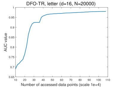
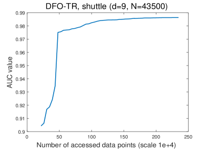
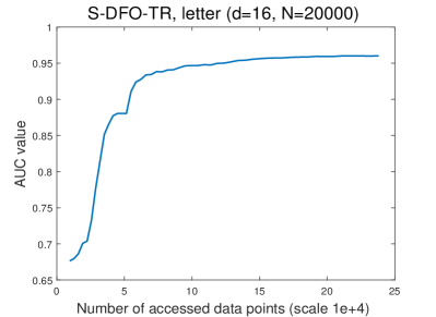
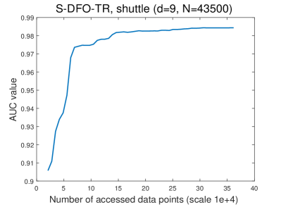
Figure 1: Comparison of stochastic DFO-TR and deterministic one in optimizing AUC function.

5.3 Hyperparameter Tuning of Cost-Sensitive RBF-Kernel SVM

Finally, we turn to hyperparamater tuning to show that DFO-TR can also outperform state-of-the-art methods on this problem. We consider tuning parameters of an RBF-kernel, cost-sensitive, SVM, with $\ell_{2}$ regularization parameter $\lambda$, kernel width $\gamma$, and positive class cost $c_{p}$. Thus, in this setting, we compare the performance of DFO-TR, random search, and Bayesian optimization algorithms, in tuning a three-dimensional hyperparameter $w=(\lambda,\gamma,{c_{p}})$, in order to achieve a high test accuracy.

For the random search algorithm, as well as the Bayesian optimization algorithms, the search space is chosen as $\lambda\in[10^{-6},10^{0}]$, $\gamma\in[10^{0},10^{3}]$, as is done in (Jamieson & Talwalkar, 2015), and $c_{p}\in[10^{-2},10^{2}]$. The setting of Algorithm 1 is as described in §5.1, while $w_{0}=(\lambda_{0},\gamma_{0},{c_{p}}_{0})$ is a three-dimensional vector randomly drawn from the search space defined above.

We have used the five-fold cross-validation with the train-validate-test framework as follows: we used two folds as the training set for the SVM model, other two folds as the validation set to compute and maximize the validation accuracy, and the remaining one as the test set to report the test accuracy.

Figure 2 illustrates the performance of DFO-TR versus random search and Bayesian optimization algorithms, in terms of the average test accuracy over the number of function evaluations. As we can see, DFO-TR constantly surpasses random search and Bayesian optimization algorithms. It is worth mentioning that random search is competitive with the BO methods and in contrast to §5.1 and §5.2, SMAC performs the best among the Bayesian optimization algorithms.

Figure 2: Comparison of DFO-TR, random search and BO algorithms on tuning RBF-kernel SVM hyperparameters.

6 Conclusion

In this work, we demonstrate that model-based derivative free optimization is a better alternative to Bayesian optimization for some black-box optimization tasks arising in machine learning. We rely on an existing convergent stochastic trust region framework to provide theoretical foundation for the chosen algorithm, and we demonstrate the efficiency of a practical implementation of DFO-TR for optimizing AUC function over the set of linear classifiers, hyperparameter tuning, and on other benchmark problems.

Appendix

In this section, we provide some complementary results. Table 7 compares the performance of the linear classifier obtained by directly maximizing AUC via DFO-TR, versus approximately maximizing AUC by utilizing gradient descent approach to minimize the pair-wise hinge loss. We utilized the same strategy of using data sets as is done in §5.2.1. Therefore, the AUC value in Table 7 is the average AUC value of 20 different runs. As we can see, compared to minimizing pair-wise hinge loss, DFO-TR achieves competitive AUC value in less number of function evaluations.

Figures 3 and 4 support the computational results in §5.2 and illustrate the per iteration behavior of each method. We can see that DFO improves the objective values faster than the Bayesian optimization algorithms.

Table 7: Comparing deterministic DFO-TR vs. pairwise hinge loss minimization

Algorithm	fourclass		svmguide1
	AUC	num. fevals	AUC	num. fevals
Pair-Wise Hinge	0.836226$\pm$ 0.000923	480	0.989319 $\pm$ 0.000008	334
DFO-TR	0.836311$\pm$ 0.000921	254	0.989132$\pm$ 0.000007	254
Algorithm	diabetes		shuttle
	AUC	num. fevals	AUC	num. fevals
Pair-Wise Hinge	0.830852$\pm$0.001015	348	0.988625$\pm$0.000021	266
DFO-TR	0.830402$\pm$0.00106	254	0.987531$\pm$0.000035	254
Algorithm	vowel		magic04
	AUC	num. fevals	AUC	num. fevals
Pair-Wise Hinge	0.975586$\pm$0.000396	348	0.843085 $\pm$ 0.000208	417
DFO-TR	0.973785$\pm$0.000506	254	0.843511$\pm$0.000213	254
Algorithm	letter		segment
	AUC	num. fevals	AUC	num. fevals
Pair-Wise Hinge	0.986699$\pm$0.000037	517	0.993134 $\pm$ 0.000023	753
DFO-TR	0.985119$\pm$0.000042	254	0.99567$\pm$0.00071	254
Algorithm	ijcnn1		svmguide3
	AUC	num. fevals	AUC	num. fevals
Pair-Wise Hinge	0.930685$\pm$0.000204	413	0.793116$\pm$0.001284	368
DFO-TR	0.910897$\pm$ 0.000264	254	0.775246$\pm$ 0.002083	254
Algorithm	german		satimage
	AUC	num. fevals	AUC	num. fevals
Pair-Wise Hinge	0.792402$\pm$ 0.000795	421	0.769505$\pm$0.000253	763
DFO-TR	0.791048$\pm$0.000846	254	0.757554$\pm$0.000236	254

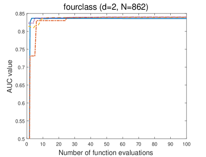
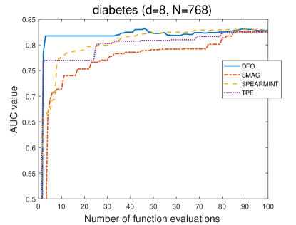
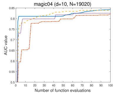
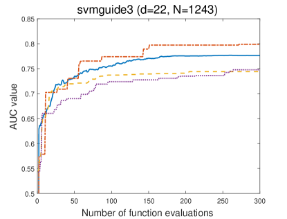
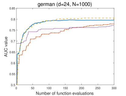
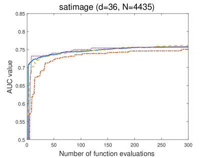
Figure 3: DFO-TR vs. BO algorithms (First Part).

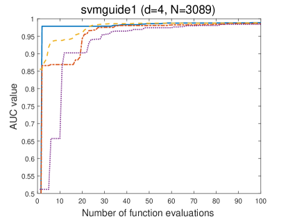
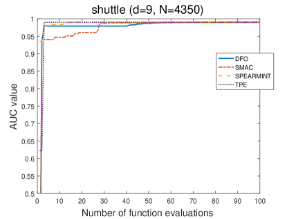
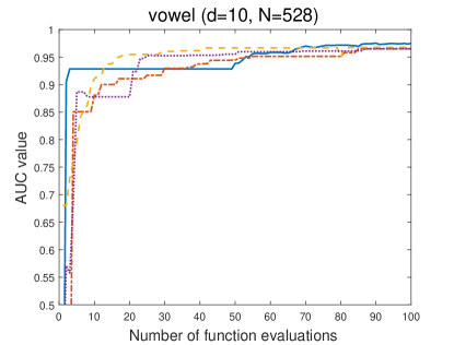
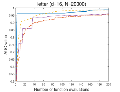
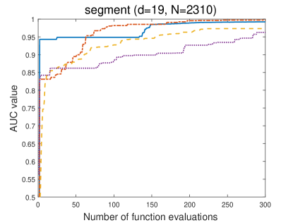
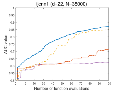
Figure 4: DFO-TR vs. BO algorithms (Second Part).

References

- Bergstra et al. (2011) Bergstra, J., Bardenet, R., Bengio, Y., and Kegl, B. Algorithms for hyper-parameter optimization. In Proc. of NIPS-11, 2011.
- Billups & Larson (2016) Billups, S. C. and Larson, J. Stochastic derivative-free optimization using a trust region framework. J. Computational Optimization and Apps, 64(2):619–645, 2016.
- Blanchet et al. (2016) Blanchet, J., Cartis, C., Menickelly, M., and Scheinberg, K. Convergence rate analysis of a stochastic trust region method for nonconvex optimization. https://arxiv.org/pdf/1609.07428, 2016.
- Bradley (1997) Bradley, A. P. The use of the area under the ROC curve in the evaluation of machine learning algorithms. Pattern Recognition, 30:1145–1159, 1997.
- Brefeld & Scheffer (2005) Brefeld, U. and Scheffer, T. AUC maximizing support vector learning. ICML, 2005.
- Brochu et al. (2010) Brochu, E., Cora, V.M., and de Freitas, N. A tutorial on Bayesian optimization of expensive cost functions, with application to active user modeling and hierarchical reinforcement learning. eprint arXiv:1012.2599, arXiv.org, 2010.
- Calders & Jaroszewicz (2007) Calders, T. and Jaroszewicz, S. Efficient AUC optimization for classification. Discovery in Databases, Warsaw, Poland, pp. 42–53, 2007.
- Chen et al. (2015) Chen, R., Menickelly, M., and Scheinberg, K. Stochastic optimization using a trust-region method and random models. https://arxiv.org/pdf/1504.04231, 2015.
- Conn et al. (1997) Conn, A. R., Scheinberg, K., and Ph. L. Toint. Recent progress in unconstrained nonlinear optimization without derivatives. Mathematical Programming, 79:397–414, 1997.
- Conn et al. (2000) Conn, A. R., Gould, N. I. M., and Toint, P. T. Trust Region Methods. MPS/SIAM Series on Optimization. SIAM, Philadelphia, 2000.
- Conn et al. (2009) Conn, A.R., Scheinberg, K., and Vicente, L.N. Introduction To Derivative-Free Optimization. Society for Industrial and Applied Mathematics. Philadelphia, 2009.
- Cortes & Mohri (2004) Cortes, C. and Mohri, M. AUC optimization vs. error rate minimization. In S. Thrun, L. Saul, and B. Scholkopf, editors, Advances in Neural Information Processing Systems 16. MIT Press, Cambridge, MA, 2004.
- Eggensperger et al. (2013) Eggensperger, K., Feurer, M., Hutter, F., Bergstra, J., Snoek, J., Hoos, H. H., and Brown, K. L. Towards an empirical foundation for assessing bayesian optimization of hyperparameters. In NIPS Workshop on Bayesian Optimization in Theory and Practice, 2013.
- Ferri et al. (2002) Ferri, C., Flach, P., and Hernandez-Orallo, J. Learning decision trees using the area under the ROC curve. ICML, 2002.
- Hanley & McNeil (1982) Hanley, J. A. and McNeil, B. J. The meaning and use of the area under a receiver operating characteristic (ROC) curve. Radiology, 1982.
- Herschtal & Raskutti (2004) Herschtal, A. and Raskutti, B. Optimizing area under the ROC curve using gradient descent. In ICML, ACM Press, New York, 2004.
- Hutter et al. (2011) Hutter, F., Hoos, H. H., and Leyton-Brown, K. Sequential model-based optimization for general algorithm configuration. In Proc. of LION-5, 2011.
- Jamieson & Talwalkar (2015) Jamieson, Kevin and Talwalkar, Ameet. Non-stochastic best arm identification and hyperparameter optimization. https://arxiv.org/pdf/1502.07943, 2015.
- Joachims (2006) Joachims, T. Training linear SVMs in linear time. In ACM SIGKDD, pp. 217–226, 2006.
- Jones et al. (1993) Jones, D. R., Perttunen, C. D., and Stuckman, B. E. Lipschitzian optimization without the lipschitz constant. J. Optimization Theory and Apps, 79:157–181, 1993.
- Jones et al. (1998) Jones, D. R., Schonlau, M., and Welch, W. J. Efficient global optimization of expensive black-box functions. J. Global Optimization, 13:455–492, 1998.
- Li et al. (2016) Li, L., Jamieson, K., DeSalvo, G., Rostamizadeh, A., and Talwalkar, A. Hyperband: A novel bandit-based approach to hyperparameter optimization. https://arxiv.org/abs/1603.06560, 2016.
- Lu et al. (2010) Lu, X., Tang, K., and Yao, X. Evolving neural networks with maximum AUC for imbalanced data classification. LNAI, 6076:335–342, 2010.
- M. Schonlau & Jones (1998) M. Schonlau, W. J. Welch and Jones, D. R. Global versus local search in constrained optimization of computer models. In New Developments and Applications in Experimental Design, 34:11–25, 1998.
- Mann & Whitney (1947) Mann, H. B. and Whitney, D. R. On a test whether one of two random variables is stochastically larger than the other. Ann. Math. Statist, 18:50–60, 1947.
- Mockus (1994) Mockus, J. Application of bayesian approach to numerical methods of global and stochastic optimization. J. Global Optimization, 4:347–365, 1994.
- More & Wild (2009) More, J. J. and Wild, S. M. Benchmarking derivative-free optimization algorithms. SIAM J. Optim, 20:172–191, 2009.
- Powell (2004) Powell, M. J. D. Least Frobenius norm updating of quadratic models that satisfy interpolation conditions. Mathematical Programming, 100:183–215, 2004.
- Rudin & Schapire (2009) Rudin, C. and Schapire, R. E. Margin-based ranking and an equivalence between adaboost and rankboost. Journal of Machine Learning Research, 10:2193–2232, 2009.
- Scheinberg & Toint (2010) Scheinberg, K. and Toint, Ph. L. Self-correcting geometry in model-based algorithms for derivative-free unconstrained optimization. SIAM J. Optim, 20(6):3512–3532, 2010.
- Shashaani et al. (2015) Shashaani, S., Hashemi, F. S., and Pasupathy, R. ASTRO-DF: A class of adaptive sampling trust-region algorithms for derivative-free simulation optimization. https://arxiv.org/pdf/1610.06506, 2015.
- Snoek et al. (2012) Snoek, J., Larochelle, H., and Adams, R.P. Practical bayesian optimization of machine learning algorithms. In Proc. of NIPS-12, 2012.
- Steck (2007) Steck, H. Hinge rank loss and the area under the ROC curve. In ECML, Lecture Notes in Computer Science, pp. 347–358, 2007.
- Tong (1990) Tong, Y.L. The multivariate normal distribution. Springer Series in Statistics, 1990.
- Yan et al. (2003) Yan, L., Dodier, R., Mozer, M.C., and Wolniewicz, R. Optimizing classifier performance via approximation to the wilcoxon-mann-witney statistic. Proceedings of the Twentieth Intl. Conf. on Machine Learning, AAAI Press, Menlo Park, CA, pp. 848–855, 2003.
- Zhao et al. (2011) Zhao, P., Hoi, S. C. H., Jin, R., and Yang, T. Online AUC maximization. In Proceedings of the 28th ICML, Bellevue, WA, USA, 2011.