Non-robust phase transitions in the generalized clock model on trees

C. Külske, P. Schriever C. Külske
Fakultät für Mathematik, Ruhr-University of Bochum, Postfach 102148,  44721, Bochum, Germany
Christof.Kuelske@ruhr-uni-bochum.de P. Schriever
Fakultät für Mathematik, Ruhr-University of Bochum, Postfach 102148,  44721, Bochum, Germany
Philipp.Schriever-d8j@ruhr-uni-bochum.de
Abstract.

Pemantle and Steif provided a sharp threshold for the existence of a RPT (robust phase transition) for the continuous rotator model and the Potts model in terms of the branching number and the second eigenvalue of the transfer operator, where a robust phase transition is said to occur if an arbitrarily weak coupling with symmetry-breaking boundary conditions suffices to induce symmetry breaking in the bulk. They further showed that for the Potts model RPT occurs at a different threshold than PT (phase transition in the sense of multiple Gibbs measures), and conjectured that RPT and PT should occur at the same threshold in the continuous rotator model.

We consider the class of 444- and 555-state rotation-invariant spin models with reflection symmetry on general trees which contains the Potts model and the clock model with scalarproduct-interaction as limiting cases. The clock model can be viewed as a particular discretization which is obtained from the classical rotator model with state space S1superscript𝑆1S^{1}.

We analyze the transition between PT=RPT and PT\neqRPT, in terms of the eigenvalues of the transfer matrix of the model at the critical threshold value for the existence of RPT. The transition between the two regimes depends sensitively on the third largest eigenvalue.

Mathematics Subject Classifications (2010). 82B26 (primary); 60K35 (secondary)

Key words. Trees, Gibbs measures, phase transition, robust phase transition, clock model, XY-model.

1. Introduction

We consider spin models on locally finite trees T=(V,E)𝑇𝑉𝐸T=(V,E) where the spin variables σx,xVsubscript𝜎𝑥𝑥𝑉\sigma_{x},x\in V, take values in the finite local state space Ω0={0,,q1}subscriptΩ00𝑞1\Omega_{0}=\{0,...,q-1\}, q𝑞q\in\mathbb{N}. The interaction between the spin variables will be given by a transfer matrix which is circulant, i.e. possesses discrete rotation-invariance, and which can therefore be uniquely described by its eigenvalues. An interesting question is whether or not there exists more than one extremal Gibbs measure, i.e., if there is a phase transition for this model. A little bit more involved is the question if it is possible to identify precise values for the free parameters of the transfer matrix at which a phase transition occurs. For background and recent results see [1, 2, 11, 14, 16, 17, 21, 22, 23, 28, 32].
Another interest in spin models on trees comes from network theory, where random graphs are used to describe the interaction between different agents. In these models the random graphs are often assumed (or proven in the large-graph limit) to be locally tree-like. To understand the behavior of these systems it is important to understand the situation on the tree first [4, 5, 6, 7].

For the Ising model on an arbitrary infinite tree with constant interaction strength J𝐽J the exact critical inverse temperature βcsubscript𝛽𝑐\beta_{c} of phase transition is well-known and is given by Jβc=kcoth1(brT)𝐽subscript𝛽𝑐𝑘superscripthyperbolic-cotangent1br𝑇J\beta_{c}=k\coth^{-1}(\operatorname{br}T), where k𝑘k is Boltzmann’s constant and brTbr𝑇\operatorname{br}T is the branching number of the tree which captures the average number of edges per vertex [25]. Similarly, the critical value for the existence of infinite clusters under independent Bernoulli percolation and the critical value for recurrence of random walks on the tree are given in terms of brTbr𝑇\operatorname{br}T as well [26].

One way to determine whether or not the spin model exhibits a phase transition is to exploit the recursion formula for the marginal distributions of the finite-volume Gibbs measures under boundary condition, see (3.1). For such models there is no phase transition, if and only if all the single-site marginals of the finite-volume Gibbs measures converge to the equidistribution for every boundary condition ωΩ𝜔Ω\omega\in\Omega (Proposition 3.1). For some models which are stochastically increasing in the boundary condition, in a sense described below, it is even enough to prove that the marginals of the finite-volume Gibbs measure under plus boundary condition converge to the equidistribution. This is for example the case in the Ising and the continuous rotator model, but also in the generalized clock model which will be introduced shortly (Proposition 3.2).

Showing that the Gibbs marginals converge under the tree recursion is in general a challenging problem: Along the leaves of the finite subtree we have to fix a boundary condition, which means that we are starting from a Dirac distribution, i.e., far away from the equidistribution, and the recursion, in general, lacks any convexity.

In [29] Pemantle and Steif introduced the notion of a robust phase transition (or RPT) which makes the tree recursion for the Gibbs marginals easier to analyze. Such a robust phase transition is said to occur when even for an arbitrary weakening of the interaction along the spins at the boundary of a sequence of finite sub-volumes ΛnSSVsubscriptΛ𝑛SS𝑉\Lambda_{n}\SS V, we still retain information about the spins at a single site in the thermodynamic limit n𝑛n\to\infty, i.e., even under this stronger condition the single-site Gibbs marginals are not converging to the equidistribution. For more background on phase-transitions in systems with weak boundary couplings see also [9, 10]. The question whether or not there is a robust phase transition is easier to answer as one can make use of local arguments around the equidistribution. To be more specific: Under the assumption that there is a robust phase transition it is possible to start the recursion in a distribution which is already arbitrarily close to the equidistribution. Then, we only have to make sure that under the recursion we are repelled from the equidistribution. The behavior is heuristically understood in terms of the linearization of the recursion, but to control the non-linearities along relevant directions is delicate.

Pemantle and Steif provided a sharp threshold for the existence of a RPT for the continuous rotator model (also called classical Heisenberg model) in any dimension, as well as for the Potts model. Similarly to the threshold for regular phase transitions in the Ising model, it is given in terms of the branching number of the tree and an effective coupling parameter, which turns out to be the second eigenvalue of the transfer operator. Furthermore they showed that for the Potts model RPT occurs at a different threshold than the regular phase transition, but conjectured that RPT and regular phase transition should occur at the same threshold in the continuous Heisenberg models [29]. It is therefore interesting to investigate generalized clock models as interpolations between the Potts model and the model of plane rotators (XY-model, Heisenberg model on S1superscript𝑆1S^{1}), from the perspective of the study of RPTs. (For more results around the issue of differences and similarities between continuous spin-models and clock models see e.g. [13, 27, 12, 19].)

This paper consists of two main parts:

Applicability of Pemantle-Steif theory:
We consider a class of finite-state spin models on general trees and show that for a wide range of circulant transfer matrices the sharp threshold for the existence of RPT given by Pemantle and Steif holds in these cases as well (Proposition 2.5). More precisely, this result holds under the assumption that the matrix elements of the transfer matrix are non-increasing in the distance to the diagonal. This is equivalent to saying that the pair potential describing the interaction of two neighboring spins along the tree is non-decreasing in the difference of the spin values along the discrete circle.

Bifurcation analysis on binary tree for q=4,5𝑞45q=4,5:
For q=4,5𝑞45q=4,5 we show that in these models, which we call generalized clock models, RPT and regular phase transition are in general not equivalent and we determine the transition point between both scenarios in terms of the third eigenvalue of the corresponding transfer operator for two examples on the binary tree (Theorem 2.6). For a visualization of the regions of the different regimes see Figures 5, 6 in Section 4. In the standard clock model with cosine-potential it turns out that there are no non-robust phase transitions (unlike q=3𝑞3q=3).
The non-equivalence is shown by studying the tree recursion on the level of the Fourier coefficients α1,α2subscript𝛼1subscript𝛼2\alpha_{1},\alpha_{2} of the marginal distributions of the finite-volume Gibbs measures. This leads us to a two-dimensional fixed-point equation which turns out to be polynomial. The number of solutions to this fixed-point equation can then be given by analytic arguments.

2. The generalized clock model: Definitions and main results

Let T=(V,E)𝑇𝑉𝐸T=(V,E) be a locally finite tree with vertex set V𝑉V and edge set E𝐸E which is rooted at some vertex oV𝑜𝑉o\in V. The number of neighbors of the vertices is assumed to be bounded by a finite constant B𝐵B throughout. Let dG:V×V:subscript𝑑𝐺𝑉𝑉d_{G}:V\times V\to\mathbb{N} be the graph distance on T𝑇T, i.e., dG(x,y)subscript𝑑𝐺𝑥𝑦d_{G}(x,y) equals the number of edges in the shortest path from x𝑥x to y𝑦y for each pair x,yV𝑥𝑦𝑉x,y\in V. Also, let |x|:=dG(x,o)assign𝑥subscript𝑑𝐺𝑥𝑜|x|:=d_{G}(x,o) for any xV𝑥𝑉x\in V. Two vertices v𝑣v and w𝑤w are called nearest neighbors if dG(v,w)=1subscript𝑑𝐺𝑣𝑤1d_{G}(v,w)=1, i.e., if there exists an edge eE𝑒𝐸e\in E connecting them. We use the notation e={v,w}𝑒𝑣𝑤e=\{v,w\}. We write vw𝑣𝑤v\to w if dG(v,w)=1subscript𝑑𝐺𝑣𝑤1d_{G}(v,w)=1 and |w|=|v|+1𝑤𝑣1|w|=|v|+1, i.e., v𝑣v is the parent of w𝑤w. Finite subsets ΛΛ\Lambda of V𝑉V will be denoted by ΛSSVΛSS𝑉\Lambda\SS V.

Every vertex vV𝑣𝑉v\in V will be equipped with a spin variable σvsubscript𝜎𝑣\sigma_{v} taking values in the finite metric space (Ω0,d)subscriptΩ0𝑑(\Omega_{0},d), where Ω0:={0,,q1}assignsubscriptΩ00𝑞1\Omega_{0}:=\{0,...,q-1\} and d(k,l):=1cos(2π(kl)/q)assign𝑑𝑘𝑙12𝜋𝑘𝑙𝑞d(k,l):=1-\cos\big{(}2\pi(k-l)/q\big{)}. Let G:=qassign𝐺subscript𝑞G:=\mathbb{Z}_{q} be the cyclic group acting transitively on Ω0subscriptΩ0\Omega_{0}. Some |Ω0|×|Ω0|subscriptΩ0subscriptΩ0|\Omega_{0}|\times|\Omega_{0}| probability transition matrix M𝑀M is chosen, s.t.

M(k,l)=M(gk,gl)k,lΩ0,gG,formulae-sequence𝑀𝑘𝑙𝑀𝑔𝑘𝑔𝑙for-all𝑘formulae-sequence𝑙subscriptΩ0for-all𝑔𝐺M(k,l)=M(g\circ k,g\circ l)\quad\forall k,l\in\Omega_{0},\;\forall g\in G,

and M(0,j)=M(0,k)𝑀0𝑗𝑀0𝑘M(0,j)=M(0,k) if d(0,j)=d(0,k)𝑑0𝑗𝑑0𝑘d(0,j)=d(0,k). We will further assume that M𝑀M is non-increasing, i.e., M(i,j)M(k,l)𝑀𝑖𝑗𝑀𝑘𝑙M(i,j)\leq M(k,l) if d(i,j)d(k,l)𝑑𝑖𝑗𝑑𝑘𝑙d(i,j)\geq d(k,l). Due to the Perron-Frobenius theorem the stochastic matrix M𝑀M has the distinguished eigenvalue λ0=1subscript𝜆01\lambda_{0}=1 with the following properties: First, |λ|<λ0𝜆subscript𝜆0|\lambda|<\lambda_{0} for all eigenvalues λλ0𝜆subscript𝜆0\lambda\neq\lambda_{0} of M𝑀M, and secondly, λ0subscript𝜆0\lambda_{0} is simple. We note that because M𝑀M is invariant under the G𝐺G-action the matrix is circulant and can hence be completely described by its first row, which will be denoted by r𝑟r.

As M𝑀M is a transfer matrix (which even happens to be a stochastic matrix the way we have defined it) we can define an associated potential Φ(i,j)Φ𝑖𝑗\Phi(i,j) by letting

Φ(i,j):=logM(i,j)assignΦ𝑖𝑗𝑀𝑖𝑗\begin{split}\Phi(i,j):=-\log M(i,j)\end{split}

and define the corresponding formal infinite-volume Hamiltonian by

H(ω)={v,w}EΦ(ωv,ωw).𝐻𝜔subscript𝑣𝑤𝐸Φsubscript𝜔𝑣subscript𝜔𝑤\begin{split}H(\omega)=\sum_{\{v,w\}\in E}\Phi(\omega_{v},\omega_{w}).\end{split}

We call a spin model with such a Hamiltonian a generalized clock model. Using inverse discrete Fourier transformation we can describe the circulant transfer matrix M𝑀M (and the potential ΦΦ\Phi accordingly) also by its eigenvalues. Remember that the eigenvalues λjsubscript𝜆𝑗\lambda_{j} of M𝑀M are given by

λj=k=0q1rke2πijk/q,j{0,,q1}formulae-sequencesubscript𝜆𝑗superscriptsubscript𝑘0𝑞1subscript𝑟𝑘superscript𝑒2𝜋𝑖𝑗𝑘𝑞𝑗0𝑞1\lambda_{j}=\sum_{k=0}^{q-1}r_{k}e^{-2\pi ijk/q},\quad j\in\{0,...,q-1\}

and the first row of M𝑀M is then recovered by

rl=1qk=0q1λke2πilk/q,l{0,,q1}.formulae-sequencesubscript𝑟𝑙1𝑞superscriptsubscript𝑘0𝑞1subscript𝜆𝑘superscript𝑒2𝜋𝑖𝑙𝑘𝑞𝑙0𝑞1r_{l}=\frac{1}{q}\sum_{k=0}^{q-1}\lambda_{k}e^{2\pi ilk/q},\quad l\in\{0,...,q-1\}.

If the eigenvalues are chosen such that M𝑀M is of the form

Mi,j={eJ/Z,if i=j1/Z,if ijsubscript𝑀𝑖𝑗casessuperscript𝑒𝐽𝑍if 𝑖𝑗1𝑍if 𝑖𝑗M_{i,j}=\left\{\begin{array}[]{cl}e^{J}/Z,&\mbox{if }i=j\\ 1/Z,&\mbox{if }i\neq j\end{array}\right.

where J>0𝐽0J>0 suitable and Z>0𝑍0Z>0 is a normalizing constant, we recover the Potts model. If M𝑀M is given by

Mi,j=1ZeJcos(2π(ij)/q),subscript𝑀𝑖𝑗1𝑍superscript𝑒𝐽2𝜋𝑖𝑗𝑞M_{i,j}=\frac{1}{Z}e^{J\cos(2\pi(i-j)/q)},

for some J>0𝐽0J>0 and normalizing constant Z>0𝑍0Z>0, we recover the standard-clock model with scalarproduct-interaction.

A cutset C𝐶C is a finite set of vertices such that every self-avoiding infinite path starting from the root o𝑜o intersects C𝐶C such that there are no vertices x,yC𝑥𝑦𝐶x,y\in C with |x|<|y|𝑥𝑦|x|<|y| and x𝑥x lies in the shortest path from o𝑜o to y𝑦y. For a cutset C𝐶C the graph TC𝑇𝐶T\setminus C consists of some infinite components and one finite component. The finite component will be denoted by Cisuperscript𝐶𝑖C^{i} and the union of the infinite components of TC𝑇𝐶T\setminus C will be denoted by Cosuperscript𝐶𝑜C^{o}. A sequence of cutsets {Cn}nsubscriptsubscript𝐶𝑛𝑛\{C_{n}\}_{n\in\mathbb{N}} is said to exhaust V, if for every vertex vV𝑣𝑉v\in V there exists a N𝑁N\in\mathbb{N} s.t. vCni𝑣superscriptsubscript𝐶𝑛𝑖v\in C_{n}^{i} for every nN𝑛𝑁n\geq N. We define the configuration space by Ω=Ω0VΩsuperscriptsubscriptΩ0𝑉\Omega=\Omega_{0}^{V}.

Definition 2.1.

Let C𝐶C be a cutset of the tree T𝑇T and δΩ𝛿Ω\delta\in\Omega a spin configuration which serves as a boundary condition to the interior. The finite-volume Gibbs measure on Ω0CisuperscriptsubscriptΩ0superscript𝐶𝑖\Omega_{0}^{C^{i}} under boundary condition δ𝛿\delta is defined by

(2.1) μCΦ,δ(ωCi)=1ZCΦ(δ)exp(HCΦ,δ(ωCi)),superscriptsubscript𝜇𝐶Φ𝛿subscript𝜔superscript𝐶𝑖1superscriptsubscript𝑍𝐶Φ𝛿superscriptsubscript𝐻𝐶Φ𝛿subscript𝜔superscript𝐶𝑖\mu_{C}^{\Phi,\delta}(\omega_{C^{i}})=\frac{1}{Z_{C}^{\Phi}(\delta)}\exp\Big{(}-H_{C}^{\Phi,\delta}(\omega_{C^{i}})\Big{)},

where

HCΦ,δ(ωCi)={x,y}E:x,yCiΦ(ωx,ωy)+{x,y}E:xCi,yCΦ(ωx,δy)superscriptsubscript𝐻𝐶Φ𝛿subscript𝜔superscript𝐶𝑖subscript:𝑥𝑦𝐸absent𝑥𝑦superscript𝐶𝑖Φsubscript𝜔𝑥subscript𝜔𝑦subscript:𝑥𝑦𝐸absentformulae-sequence𝑥superscript𝐶𝑖𝑦𝐶Φsubscript𝜔𝑥subscript𝛿𝑦H_{C}^{\Phi,\delta}(\omega_{C^{i}})=\sum_{\begin{subarray}{c}\{x,y\}\in E:\\ x,y\in C^{i}\end{subarray}}\Phi(\omega_{x},\omega_{y})+\sum_{\begin{subarray}{c}\{x,y\}\in E:\\ x\in C^{i},y\in C\end{subarray}}\Phi(\omega_{x},\delta_{y})

and

ZCΦ(δ)=ω~CiΩ0Ciexp(HCΦ,δ(ω~Ci))superscriptsubscript𝑍𝐶Φ𝛿subscriptsubscript~𝜔superscript𝐶𝑖superscriptsubscriptΩ0superscript𝐶𝑖subscriptsuperscript𝐻Φ𝛿𝐶subscript~𝜔superscript𝐶𝑖Z_{C}^{\Phi}(\delta)=\sum_{\tilde{\omega}_{C^{i}}\in\Omega_{0}^{C^{i}}}\exp\Big{(}-H^{\Phi,\delta}_{C}(\tilde{\omega}_{C^{i}})\Big{)}

is a normalizing constant or partition function. If the second summand in the Hamiltonian H𝐻H is left out, i.e., if there is no interaction with the boundary, we call this the free Gibbs measure.

Note that the family of finite-volume Gibbs measures as we have defined them above can also be interpreted as a (local) Gibbsian specification γΦsuperscript𝛾Φ\gamma^{\Phi} [18, Definition 1.23] which is given by

(2.2) γCiΦ(fδ)=μCΦ,δ(dωCi)f(ωCiδ(Ci)c).subscriptsuperscript𝛾Φsuperscript𝐶𝑖conditional𝑓𝛿superscriptsubscript𝜇𝐶Φ𝛿𝑑subscript𝜔superscript𝐶𝑖𝑓subscript𝜔superscript𝐶𝑖subscript𝛿superscriptsuperscript𝐶𝑖𝑐\gamma^{\Phi}_{C^{i}}(f\mid\delta)=\int\mu_{C}^{\Phi,\delta}(d\omega_{C^{i}})f(\omega_{C^{i}}\delta_{(C^{i})^{c}}).

This specification is a family of probability kernels with the property that γCiΦ(δ)1(Ω0V)\gamma^{\Phi}_{C^{i}}(\cdot\mid\delta)\in\mathcal{M}_{1}(\Omega_{0}^{V}) for every δΩ𝛿Ω\delta\in\Omega and s.t. γCiΦ(A)subscriptsuperscript𝛾Φsuperscript𝐶𝑖conditional𝐴\gamma^{\Phi}_{C^{i}}(A\mid\cdot) is measurable w.r.t. the sigma-algebra generated by the spin variables {σv,v(Ci)c}subscript𝜎𝑣𝑣superscriptsuperscript𝐶𝑖𝑐\{\sigma_{v},v\in(C^{i})^{c}\} for every A(𝒫(q))V𝐴superscript𝒫subscript𝑞𝑉A\in(\mathcal{P}(\mathbb{Z}_{q}))^{V}.

Let a measure space (X,X,μ)𝑋subscript𝑋𝜇(X,\mathcal{F}_{X},\mu), a measurable space (Y,Y)𝑌subscript𝑌(Y,\mathcal{F}_{Y}) and a probability kernel π𝜋\pi from Xsubscript𝑋\mathcal{F}_{X} to Ysubscript𝑌\mathcal{F}_{Y} be given. Then the push-forward of μ𝜇\mu under π𝜋\pi is defined by

μπ(A)=μ(dω)π(Aω)AY.formulae-sequence𝜇𝜋𝐴𝜇𝑑𝜔𝜋conditional𝐴𝜔for-all𝐴subscript𝑌\mu\pi(A)=\int\mu(d\omega)\pi(A\mid\omega)\quad\forall A\in\mathcal{F}_{Y}.

A measure μ1(Ω0V)𝜇subscript1superscriptsubscriptΩ0𝑉\mu\in\mathcal{M}_{1}(\Omega_{0}^{V}) is called a Gibbs measure w.r.t. a specification (γΛ)ΛSSVsubscriptsubscript𝛾ΛΛSS𝑉(\gamma_{\Lambda})_{\Lambda\SS V} if

μ=μγΛΛSSV.𝜇𝜇subscript𝛾Λfor-allΛSS𝑉\mu=\mu\gamma_{\Lambda}\quad\forall\Lambda\SS V.

The probability kernels given by (2.2)italic-(2.2italic-)\eqref{GibbsSpec} are only defined for finite sub-volumes ΛSSVΛSS𝑉\Lambda\SS V of the specific form Λ=CiΛsuperscript𝐶𝑖\Lambda=C^{i} where C𝐶C is a cutset, but this is not an issue w.r.t. identifying the set of Gibbs measures:

Lemma 2.2.

Suppose γ𝛾\gamma is a specification and μ𝜇\mu a measure on Ω0VsuperscriptsubscriptΩ0𝑉\Omega_{0}^{V}. Then the following statements are equivalent:

  1. (i)

    μ𝜇\mu is a Gibbs measure.

  2. (ii)

    μγΛ=μ𝜇subscript𝛾Λ𝜇\mu\gamma_{\Lambda}=\mu for every ΛSSVΛSS𝑉\Lambda\SS V.

  3. (iii)

    μγCi=μ𝜇subscript𝛾superscript𝐶𝑖𝜇\mu\gamma_{C^{i}}=\mu for every cutset CSSV𝐶SS𝑉C\SS V.

For a proof, see [18, Remark 1.24]. This lemma allows us to give an alternative characterization of Gibbs measures (in the infinite volume) as follows:

Lemma 2.3.

A probability measure μ𝜇\mu in the infinite volume Ω0VsuperscriptsubscriptΩ0𝑉\Omega_{0}^{V} is called a Gibbs measure for the potential ΦΦ\Phi if for any cutset C𝐶C the conditional distribution on Cisuperscript𝐶𝑖C^{i} given a boundary configuration δΩ0V𝛿superscriptsubscriptΩ0𝑉\delta\in\Omega_{0}^{V} is given by μCΦ,δsuperscriptsubscript𝜇𝐶Φ𝛿\mu_{C}^{\Phi,\delta}, i.e.,

μ(ωCiδCCo)=μCΦ,δ(ωCi).𝜇conditionalsubscript𝜔superscript𝐶𝑖subscript𝛿𝐶superscript𝐶𝑜superscriptsubscript𝜇𝐶Φ𝛿subscript𝜔superscript𝐶𝑖\mu(\omega_{C^{i}}\mid\delta_{C\cup C^{o}})=\mu_{C}^{\Phi,\delta}(\omega_{C^{i}}).

Given an interaction potential ΦΦ\Phi, a cutset C𝐶C and a boundary condition δ𝛿\delta, let pC,oΦ,δsuperscriptsubscript𝑝𝐶𝑜Φ𝛿p_{C,o}^{\Phi,\delta} denote the marginal distribution of the finite-volume Gibbs measure μCΦ,δsuperscriptsubscript𝜇𝐶Φ𝛿\mu_{C}^{\Phi,\delta} at the root o.𝑜o. We now come to the key definition of a robust phase transition, which is said to occur if a “plus” boundary condition retains its influence on the root even when the interaction along the edges at the boundary is made arbitrarily small: Given ΦΦ\Phi and u(0,1]𝑢01u\in(0,1] and a cutset C𝐶C of T𝑇T, let Φ¯(u,C)¯Φ𝑢𝐶\bar{\Phi}(u,C) be the potential which is ΦΦ\Phi on edges in Cisuperscript𝐶𝑖C^{i} and uΦ𝑢Φu\Phi on edges connecting C𝐶C to Cisuperscript𝐶𝑖C^{i}. Let δ0subscript𝛿0\delta_{0} be a boundary configuration which is all 00, i.e., (δ0)v=0subscriptsubscript𝛿0𝑣0(\delta_{0})_{v}=0 for all vV𝑣𝑉v\in V. Let pC,ou,Φ,+superscriptsubscript𝑝𝐶𝑜𝑢Φp_{C,o}^{u,\Phi,+} denote the marginal distribution at the root o𝑜o of the measure μCu,Φ,+:=μCΦ¯(u,C),δ0assignsuperscriptsubscript𝜇𝐶𝑢Φsuperscriptsubscript𝜇𝐶¯Φ𝑢𝐶subscript𝛿0\mu_{C}^{u,\Phi,+}:=\mu_{C}^{\bar{\Phi}(u,C),\delta_{0}}. In the following we will always denote the equidistribution on Ω0subscriptΩ0\Omega_{0} by 𝟏1\mathbf{1}.

δ𝛿\deltaC𝐶Co𝑜ov𝑣vuΦ𝑢Φu\PhiΦΦ\Phi
Definition 2.4.

A generalized clock model on the tree T𝑇T is said to exhibit a robust phase transition for the interaction ΦΦ\Phi if for every u(0,1],𝑢01u\in(0,1],

infCpC,ou,Φ,+𝟏0,subscriptinfimum𝐶subscriptnormsuperscriptsubscript𝑝𝐶𝑜𝑢Φ10\inf_{C}||p_{C,o}^{u,\Phi,+}-\mathbf{1}||_{\infty}\neq 0,

where the infimum is taken over all cutsets C𝐶C of T𝑇T.

We will show that under a positivity assumption on the eigenvalues of the transfer matrix M𝑀M, which is chosen such that M𝑀M is non-increasing, the existence of a robust phase transition is a geometric property of the underlying tree T𝑇T. The decisive parameter in this regard is the branching number, which in some sense captures the average number of edges per vertex of the tree. It is defined by

(2.3) brT:=sup{λ:infCvCλ|v|>0},assignbr𝑇supremumconditional-set𝜆subscriptinfimum𝐶subscript𝑣𝐶superscript𝜆𝑣0\operatorname{br}T:=\sup\{\lambda:\inf_{C}\sum_{v\in C}\lambda^{-|v|}>0\},

where the infimum is once more taken over all cutsets C𝐶C.

The branching number has been introduced in this form by Lyons [26] and it can be interpreted as the exponential of the Hausdorff dimension of the boundary T𝑇\partial T of the tree which has been studied previously by Furstenberg [15]. For percolation and symmetric root-biased random walks on trees it is known that there exist sharp thresholds for the existence of infinite clusters and positive recurrence respectively that are given by the branching number [26].

The definition of robust phase transitions goes back to a paper by Pemantle and Steif [29], in which they showed that under certain “ferromagneticity” assumptions, amongst others regarding the positivity of the Fourier coefficients of the Gibbs marginals, there exists a sharp threshold for the existence of such RPTs which is given by

λ1brT=1,subscript𝜆1br𝑇1\lambda_{1}\operatorname{br}T=1,

where λ1subscript𝜆1\lambda_{1} denotes the first non-trivial Fourier coefficient of the transfer operator. By establishing applicability of the results of Pemantle and Steif we prove that this threshold holds also for certain types of generalized clock models:

Proposition 2.5.

Let T𝑇T be a tree and M𝑀M the transfer matrix of a generalized clock model with state space Ω0={0,1,,q1}subscriptΩ001𝑞1\Omega_{0}=\{0,1,...,q-1\}. Assume that all eigenvalues of M𝑀M are non-negative and such that M𝑀M is non-increasing. Let λ1subscript𝜆1\lambda_{1} be the second largest eigenvalue of M𝑀M. If

λ1brT>1subscript𝜆1br𝑇1\lambda_{1}\operatorname{br}T>1

then there is a robust phase transition and if

λ1brT<1subscript𝜆1br𝑇1\lambda_{1}\operatorname{br}T<1

there is no robust phase transition.

Remember that for suitably chosen eigenvalues for the transfer matrix M𝑀M we recover the Potts model and the standard-clock model with the potential Φ(i,j)=cos(2πq(ij))Φ𝑖𝑗2𝜋𝑞𝑖𝑗\Phi(i,j)=\cos\big{(}\frac{2\pi}{q}(i-j)\big{)} respectively from the generalized clock model. In both of these two models the same sharp threshold for the existence of a RPT as given in Theorem 2.5 holds.

The existence of a robust phase transition always implies phase transition (Proposition 3.2). However for the Potts model it is known that the existence of regular phase transitions does not solely depend on the second largest eigenvalue and the existence of a regular phase transition does not imply the existence of a RPT. For the classical Heisenberg model it has been only conjectured that robust and non-robust phase transitions do coincide [29].

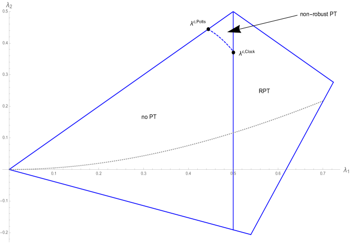
We show that in the generalized clock model there is no equivalence of PT and RPT in general: For q=4,5𝑞45q=4,5 on the binary tree we provide the exact transition point between the two regimes PT==RPT and PT\neqRPT at criticality, i.e., for λ1=1/2subscript𝜆112\lambda_{1}=1/2, in terms of the third largest eigenvalue λ2subscript𝜆2\lambda_{2}. For q=4𝑞4q=4 we give the transition points for every λ1(0,1/2)subscript𝜆1012\lambda_{1}\in(0,1/2) (see Figure 5).

Theorem 2.6.

Consider the generalized q𝑞q-state clock model on the binary rooted tree. For q=4𝑞4q=4 and q=5𝑞5q=5 there exists a non-empty region for the eigenvalues λ1,λ2subscript𝜆1subscript𝜆2\lambda_{1},\lambda_{2} of the transfer matrix M𝑀M, such that the spin system exhibits a phase transition but no robust phase transition.

3. RPT is a geometric property: Applicability of Pemantle-Steif theory for the generalized clock model on possibly irregular trees

An important property of Gibbs measures for spin models on trees is the recursive nature of their marginal distributions pC,vΦ,δsuperscriptsubscript𝑝𝐶𝑣Φ𝛿p_{C,v}^{\Phi,\delta}: Let w1,,wksubscript𝑤1subscript𝑤𝑘w_{1},...,w_{k} be the children of v𝑣v. Then

(3.1) pC,vΦ,δ(i)=1ZC,vΦ,δl=1k(j=0q1M(i,j)pC,wlΦ,δ(j)),superscriptsubscript𝑝𝐶𝑣Φ𝛿𝑖1superscriptsubscript𝑍𝐶𝑣Φ𝛿superscriptsubscriptproduct𝑙1𝑘superscriptsubscript𝑗0𝑞1𝑀𝑖𝑗superscriptsubscript𝑝𝐶subscript𝑤𝑙Φ𝛿𝑗p_{C,v}^{\Phi,\delta}(i)=\frac{1}{Z_{C,v}^{\Phi,\delta}}\prod_{l=1}^{k}\left(\sum_{j=0}^{q-1}M(i,j)p_{C,w_{l}}^{\Phi,\delta}(j)\right),

where

ZC,vΦ,δ=k=0q1l=1k(j=0q1M(k,j)pC,wΦ,δ(j))superscriptsubscript𝑍𝐶𝑣Φ𝛿superscriptsubscript𝑘0𝑞1superscriptsubscriptproduct𝑙1𝑘superscriptsubscript𝑗0𝑞1𝑀𝑘𝑗superscriptsubscript𝑝𝐶𝑤Φ𝛿𝑗Z_{C,v}^{\Phi,\delta}=\sum_{k=0}^{q-1}\prod_{l=1}^{k}\left(\sum_{j=0}^{q-1}M(k,j)p_{C,w}^{\Phi,\delta}(j)\right)

is a normalizing constant [29, Lemma 2.2]. We like to note that equation (3.1) is the defining property of so-called boundary laws or entrance laws [18], [33]. It is known that every Gibbs measure which is a tree-indexed Markov chain can be uniquely represented in terms of a boundary law (up to a positive pre-factor), and conversely that every boundary law can be used to construct a Gibbs measure which is a Markov chain [33]. Furthermore, the extremal elements of the set of Gibbs measures are necessarily Markov chains (see [18, Theorem 12.6]), and therefore spin models on trees exhibit a phase transition if and only if there exists more than one boundary law. Note that we always have the free solution, i.e., the equidistribution 𝟏1\mathbf{1}. For a recent paper showing the connection between gradient Gibbs measures and periodic boundary laws for models with non-compact local state space, see [23].

In the following we will work towards an equivalent definition of phase transition. For every neighboring pair of vertices v,wV𝑣𝑤𝑉v,w\in V we get two infinite trees when we remove the edge {v,w}𝑣𝑤\{v,w\} from E𝐸E. Let us denote the tree containing v𝑣v by Tvsubscript𝑇𝑣T_{v} and the other by Twsubscript𝑇𝑤T_{w}. For any cutset Cnsubscript𝐶𝑛C_{n} on the whole tree T𝑇T we define cutsets Cnv:=CnTvassignsuperscriptsubscript𝐶𝑛𝑣subscript𝐶𝑛subscript𝑇𝑣C_{n}^{v}:=C_{n}\cap T_{v} and Cnw:=CnTwassignsuperscriptsubscript𝐶𝑛𝑤subscript𝐶𝑛subscript𝑇𝑤C_{n}^{w}:=C_{n}\cap T_{w} on the two subtrees Tv,Twsubscript𝑇𝑣subscript𝑇𝑤T_{v},T_{w}. For any configuration δΩ𝛿Ω\delta\in\Omega we introduce boundary conditions δvsubscript𝛿𝑣\delta_{v} and δwsubscript𝛿𝑤\delta_{w} on Tvsubscript𝑇𝑣T_{v} and Twsubscript𝑇𝑤T_{w} by setting δv:=δTvassignsubscript𝛿𝑣𝛿subscript𝑇𝑣\delta_{v}:=\delta\cap T_{v} and δw:=δTwassignsubscript𝛿𝑤𝛿subscript𝑇𝑤\delta_{w}:=\delta\cap T_{w} respectively. Note that in the following we denote the marginal distributions of the finite-volume Gibbs measures on the infinite subtrees Tvsubscript𝑇𝑣T_{v} and Twsubscript𝑇𝑤T_{w} by pCnv,vΦ,δvsuperscriptsubscript𝑝superscriptsubscript𝐶𝑛𝑣𝑣Φsubscript𝛿𝑣p_{C_{n}^{v},v}^{\Phi,\delta_{v}} and pCnw,wΦ,δwsuperscriptsubscript𝑝superscriptsubscript𝐶𝑛𝑤𝑤Φsubscript𝛿𝑤p_{C_{n}^{w},w}^{\Phi,\delta_{w}} respectively. These are not to be confused with the marginals of the finite-volume Gibbs measure on the whole tree T𝑇T. Let the inner boundary of a subset ΛVΛ𝑉\Lambda\subset V be defined by iΛ:={vΛ:wΛ with {v,w}E}assignsuperscript𝑖Λconditional-set𝑣Λ𝑤Λ with 𝑣𝑤𝐸\partial^{i}\Lambda:=\{v\in\Lambda:\exists w\in\partial\Lambda\mbox{ with }\{v,w\}\in E\}.

Proposition 3.1.

Let (αi)iVsubscriptsubscript𝛼𝑖𝑖𝑉(\alpha_{i})_{i\in V} be a family of measures on Ω0subscriptΩ0\Omega_{0} and let {Cn}nsubscriptsubscript𝐶𝑛𝑛\{C_{n}\}_{n\in\mathbb{N}} be a sequence of cutsets that exhausts V𝑉V. Suppose that for every vV𝑣𝑉v\in V and every δΩ𝛿Ω\delta\in\Omega the marginal distribution pCnv,vΦ,δvsuperscriptsubscript𝑝superscriptsubscript𝐶𝑛𝑣𝑣Φsubscript𝛿𝑣p_{C_{n}^{v},v}^{\Phi,\delta_{v}} converges to the distribution αvsubscript𝛼𝑣\alpha_{v}. Then the thermodynamic limit of the finite-volume Gibbs measure, μ:=limnγCni(δ)\mu:=\lim_{n\to\infty}\gamma_{C_{n}^{i}}(\cdot\mid\delta), exists for any choice of δ𝛿\delta and is given by

μ(σΛ=ωΛ)=1ZΛkiΛαk(ωk)bΛMb(ωb)𝜇subscript𝜎Λsubscript𝜔Λ1subscript𝑍Λsubscriptproduct𝑘superscript𝑖Λsubscript𝛼𝑘subscript𝜔𝑘subscriptproduct𝑏Λsubscript𝑀𝑏subscript𝜔𝑏\mu(\sigma_{\Lambda}=\omega_{\Lambda})=\frac{1}{Z_{\Lambda}}\prod_{k\in\partial^{i}\Lambda}\alpha_{k}(\omega_{k})\prod_{b\subset\Lambda}M_{b}(\omega_{b})

where ΛSSVΛSS𝑉\Lambda\SS V is any finite connected set, ωΛΩ0Λsubscript𝜔ΛsuperscriptsubscriptΩ0Λ\omega_{\Lambda}\in\Omega_{0}^{\Lambda}, and ZΛsubscript𝑍ΛZ_{\Lambda} is a normalizing constant.

Proof.

The proof is done by induction on |Λ|Λ|\Lambda|. First, let Λ={v,w}Λ𝑣𝑤\Lambda=\{v,w\} with vwsimilar-to𝑣𝑤v\sim w. Remove the edge connecting v𝑣v to w𝑤w from the tree to get the two subtrees Tvsubscript𝑇𝑣T_{v} and Twsubscript𝑇𝑤T_{w} which contain v𝑣v and w𝑤w respectively. Note that by assumption

pCnv,vΦ,δv(ωv)=ωCnv,ivexp(HCnv,i(ωv,ωCnv,iv,δ(Cnv,i)cv))ωv,ωCnv,ivexp(HCnv,i(ωv,ωCnv,iv,δ(Cnv,i)cv))αv(ωv)superscriptsubscript𝑝superscriptsubscript𝐶𝑛𝑣𝑣Φsubscript𝛿𝑣subscript𝜔𝑣subscriptsubscript𝜔superscriptsubscript𝐶𝑛𝑣𝑖𝑣subscript𝐻superscriptsubscript𝐶𝑛𝑣𝑖subscript𝜔𝑣subscript𝜔superscriptsubscript𝐶𝑛𝑣𝑖𝑣subscriptsuperscript𝛿𝑣superscriptsuperscriptsubscript𝐶𝑛𝑣𝑖𝑐subscriptsubscript𝜔𝑣subscript𝜔superscriptsubscript𝐶𝑛𝑣𝑖𝑣subscript𝐻superscriptsubscript𝐶𝑛𝑣𝑖subscript𝜔𝑣subscript𝜔superscriptsubscript𝐶𝑛𝑣𝑖𝑣subscriptsuperscript𝛿𝑣superscriptsuperscriptsubscript𝐶𝑛𝑣𝑖𝑐subscript𝛼𝑣subscript𝜔𝑣p_{C_{n}^{v},v}^{\Phi,\delta_{v}}(\omega_{v})=\frac{\sum_{\omega_{C_{n}^{v,i}\setminus v}}\exp(-H_{C_{n}^{v,i}}(\omega_{v},\omega_{C_{n}^{v,i}\setminus v},\delta^{v}_{(C_{n}^{v,i})^{c}}))}{\sum_{\omega_{v},\omega_{C_{n}^{v,i}\setminus v}}\exp(-H_{C_{n}^{v,i}}(\omega_{v},\omega_{C_{n}^{v,i}\setminus v},\delta^{v}_{(C_{n}^{v,i})^{c}}))}\to\alpha_{v}(\omega_{v})

for n𝑛n\to\infty. Let g𝑔g be some test-function on Λ={v,w}Λ𝑣𝑤\Lambda=\{v,w\}. Then

γCn(g(ωv,ωw)δv,δw)=ωv,ωw1ZCnδg(ωv,ωw)Mvw(ωv,ωw)×(ωCnv,i{v}exp(HCnv,i(ωv,ωCnv,iv,δ(Cnv,i)cv)))×(ωCnw,i{w}exp(HCnw,i(ωw,ωCnw,iw,δ(Cnw,i)cw)))=1Zv,wωv,ωwg(ωv,ωw)Mvw(ωv,ωw)pCnv,vΦ,δvpCnw,wΦ,δw1Zv,wωv,ωwg(ωv,ωw)Mvw(ωv,ωw)αv(ωv)αw(ωw)\begin{split}&\gamma_{C_{n}}(g(\omega_{v},\omega_{w})\mid\delta^{v},\delta^{w})\\ =&\sum_{\omega_{v},\omega_{w}}\frac{1}{Z_{C_{n}}^{\delta}}g(\omega_{v},\omega_{w})M_{vw}(\omega_{v},\omega_{w})\\ &\qquad\times\left(\sum_{\omega_{C_{n}^{v,i}\setminus\{v\}}}\exp\left(-H_{C_{n}^{v,i}}\left(\omega_{v},\omega_{C_{n}^{v,i}\setminus v},\delta^{v}_{(C_{n}^{v,i})^{c}}\right)\right)\right)\\ &\qquad\qquad\times\left(\sum_{\omega_{C_{n}^{w,i}\setminus\{w\}}}\exp\left(-H_{C_{n}^{w,i}}\left(\omega_{w},\omega_{C_{n}^{w,i}\setminus w},\delta^{w}_{(C_{n}^{w,i})^{c}}\right)\right)\right)\\ =&\frac{1}{Z_{v,w}}\sum_{\omega_{v},\omega_{w}}g(\omega_{v},\omega_{w})M_{vw}(\omega_{v},\omega_{w})\,p_{C_{n}^{v},v}^{\Phi,\delta_{v}}\,p_{C_{n}^{w},w}^{\Phi,\delta_{w}}\\ \to&\frac{1}{Z_{v,w}}\sum_{\omega_{v},\omega_{w}}g(\omega_{v},\omega_{w})M_{vw}(\omega_{v},\omega_{w})\,\alpha_{v}(\omega_{v})\,\alpha_{w}(\omega_{w})\end{split}

for n𝑛n\to\infty. This proves the claim for volumes ΛΛ\Lambda that consist of only two sites.

Now suppose the claim holds for any sub-volume ΔVΔ𝑉\Delta\subset V with |Δ|=nΔ𝑛|\Delta|=n. Let Λ:=Δ{w}assignΛΔ𝑤\Lambda:=\Delta\cup\{w\} with wΔ𝑤Δw\in\partial\Delta and v:=wΔassign𝑣𝑤Δv:=\partial w\cap\Delta. Let g𝑔g be some test-function on ΛΛ\Lambda. Then

γCn(g(ωΛ)δv,δw)=γCn(g(ωΔ,ωj)δv,δw)=ωΔ,ωj1ZCnδg(ωΔ,ωw)Mvw(ωv,ωw)×(ωCnv,iΔ(exp(HCnv,i(ωΔ,ωCnv,iΔ),δ(Cnv,i)c)))×(ωCnw,i{w}(exp(HCnv,i(ωw,ωCnv,iw),δ(Cnw,i)c)))=1ZCnδωΔ,ωjg(ωΔ,ωj)Mvw(ωv,ωw)γCnv,i(ωΔδv)pCnw,wΦ,δw1ZΛωΔ,ωjg(ωΔ,ωj)Mvw(ωv,ωw)(kiΔ{w}αk(ωk)bΔMb(ωb))αw(ωw).\begin{split}&\gamma_{C_{n}}(g(\omega_{\Lambda})\mid\delta^{v},\delta^{w})=\gamma_{C_{n}}(g(\omega_{\Delta},\omega_{j})\mid\delta^{v},\delta^{w})\\ =&\sum_{\omega_{\Delta},\omega_{j}}\frac{1}{Z_{C_{n}}^{\delta}}g(\omega_{\Delta},\omega_{w})M_{vw}(\omega_{v},\omega_{w})\\ &\qquad\times\left(\sum_{\omega_{C_{n}^{v,i}\setminus\Delta}}\left(\exp\left(-H_{C_{n}^{v,i}}(\omega_{\Delta},\omega_{C_{n}^{v,i}\setminus\Delta}),\delta_{(C_{n}^{v,i})^{c}}\right)\right)\right)\\ &\qquad\qquad\times\left(\sum_{\omega_{C_{n}^{w,i}\setminus\{w\}}}\left(\exp\left(-H_{C_{n}^{v,i}}(\omega_{w},\omega_{C_{n}^{v,i}\setminus w}),\delta_{(C_{n}^{w,i})^{c}}\right)\right)\right)\\ =&\frac{1}{Z_{C_{n}}^{\delta}}\sum_{\omega_{\Delta},\omega_{j}}g(\omega_{\Delta},\omega_{j})M_{vw}(\omega_{v},\omega_{w})\,\gamma_{C_{n}^{v,i}}(\omega_{\Delta}\mid\delta_{v})\,p_{C_{n}^{w},w}^{\Phi,\delta_{w}}\\ \to&\frac{1}{Z_{\Lambda}}\sum_{\omega_{\Delta},\omega_{j}}g(\omega_{\Delta},\omega_{j})M_{vw}(\omega_{v},\omega_{w})\,\left(\prod_{k\in\partial^{i}\Delta\setminus\{w\}}\alpha_{k}(\omega_{k})\prod_{b\subset\Delta}M_{b}(\omega_{b})\right)\alpha_{w}(\omega_{w}).\end{split}

The last equation follows from the induction assumption. Note that γCnv,i(δv)\gamma_{C_{n}^{v,i}}(\cdot\mid\delta_{v}) is the measure on the subtree Tvsubscript𝑇𝑣T_{v} and not on the whole tree. Hence the inner boundary of ΔΔ\Delta in Tvsubscript𝑇𝑣T_{v} is not containing w𝑤w. This completes the proof. ∎

Note that Proposition 3.1 readily implies that there is no phase transition under the given assumptions: Every extremal Gibbs measure μ𝜇\mu can be given as a thermodynamic limit of a finite-volume Gibbs measure prepared with some boundary configuration which is typical for μ𝜇\mu (see [8, Proposition 2.23]). As these limits are assumed to be the same for any boundary configuration ω𝜔\omega, we find that there can only exist one extremal Gibbs measure. Therefore the spin model exhibits a phase transition if and only if the recursion equation (3.1) has more than one solution. It is even enough to study the recursion under “plus” boundary condition:

Proposition 3.2.

In the generalized clock model a phase transition occurs if and only if there exists a vertex v𝑣v and a sequence of cutsets {Cn}nsubscriptsubscript𝐶𝑛𝑛\{C_{n}\}_{n\in\mathbb{N}} such that

infnpCn,vΦ,δ0𝟏0.subscriptinfimum𝑛subscriptnormsuperscriptsubscript𝑝subscript𝐶𝑛𝑣Φsubscript𝛿010\inf_{n}\|p_{C_{n},v}^{\Phi,\delta_{0}}-\mathbf{1}\|_{\infty}\neq 0.

Proposition 3.2 also holds for the Ising, Potts and continuous rotator models. The proof for the generalized clock model is analogous to the one for the rotator model [29, Proposition 1.4]. The crucial property in these models is the positivity of the Fourier coefficients of the marginal distributions pCn,vΦ,δ0superscriptsubscript𝑝subscript𝐶𝑛𝑣Φsubscript𝛿0p_{C_{n},v}^{\Phi,\delta_{0}} (3.4) and of the transfer operator r𝑟r (3.5) which we will discus later.

Observe that the r.h.s. of (3.1) is a convolution of the different distributions of the children over the vectors in the circular matrix representing the interaction, followed by an ordinary product. We will make use of consequences of this structure regarding monotonicity below.

In the following we will show that in the generalized clock model, where we assume that the eigenvalues of the transfer matrix M𝑀M are restricted by

1λj>0,j{0,,q1},formulae-sequence1subscript𝜆𝑗0for-all𝑗0𝑞11\geq\lambda_{j}>0,\quad\forall j\in\{0,...,q-1\},

and such that M𝑀M is non-increasing, the existence of a RPT is determined by the branching number of the underlying tree and the second largest eigenvalue of the transfer matrix.

To understand the recursion (3.1) for the Gibbs marginals, it is important to note that it preserves the natural class of symmetric probability vectors which have positive Fourier (cosine-)coefficients, as we will explain now.
By P(Ω0/0)𝑃subscriptΩ00P(\Omega_{0}/0) we denote the vectors on Ω0subscriptΩ0\Omega_{0} that are symmetric to 00, i.e., f(j)=f(k)𝑓𝑗𝑓𝑘f(j)=f(k) if d(0,j)=d(0,k)𝑑0𝑗𝑑0𝑘d(0,j)=d(0,k) for any fP(Ω0/0)𝑓𝑃subscriptΩ00f\in P(\Omega_{0}/0). Note that dim(P(Ω0/0))=q2+1dimension𝑃subscriptΩ00𝑞21\dim(P(\Omega_{0}/0))=\lfloor\frac{q}{2}\rfloor+1. It will be convenient to work with the non-normalized basis ={ϕj}j=0,,q2subscriptsubscriptitalic-ϕ𝑗𝑗0𝑞2\mathcal{B}=\{\phi_{j}\}_{j=0,...,\lfloor\frac{q}{2}\rfloor}, where

ϕj(k):=cos(2πjk/q),k{0,1,,q1}.formulae-sequenceassignsubscriptitalic-ϕ𝑗𝑘2𝜋𝑗𝑘𝑞𝑘01𝑞1\phi_{j}(k):=\cos(2\pi jk/q),\quad k\in\{0,1,...,q-1\}.

This basis has the properties

(3.2) ϕiϕj=12ϕi+j+12ϕijsubscriptitalic-ϕ𝑖subscriptitalic-ϕ𝑗12subscriptitalic-ϕ𝑖𝑗12subscriptitalic-ϕ𝑖𝑗\phi_{i}\phi_{j}=\frac{1}{2}\phi_{i+j}+\frac{1}{2}\phi_{i-j}

and

(3.3) ϕiϕj=zjδijϕj,subscriptitalic-ϕ𝑖subscriptitalic-ϕ𝑗subscript𝑧𝑗subscript𝛿𝑖𝑗subscriptitalic-ϕ𝑗\phi_{i}*\phi_{j}=z_{j}\delta_{ij}\phi_{j},

where ϕiϕj(k):=lϕi(kl)ϕj(l)assignsubscriptitalic-ϕ𝑖subscriptitalic-ϕ𝑗𝑘subscript𝑙subscriptitalic-ϕ𝑖𝑘𝑙subscriptitalic-ϕ𝑗𝑙\phi_{i}*\phi_{j}(k):=\sum_{l}\phi_{i}(k-l)\phi_{j}(l) and zj=kEϕj2(k)subscript𝑧𝑗subscript𝑘𝐸superscriptsubscriptitalic-ϕ𝑗2𝑘z_{j}=\sum_{k\in E}\phi_{j}^{2}(k). We introduce a new norm ||||A||\cdot||_{A} on the space of symmetric vectors P(Ω0/0)𝑃subscriptΩ00P(\Omega_{0}/0), which is defined as the sum of the absolute values of the Fourier coefficients, i.e.,

fA:=j=0q2|aj(f)|,assignsubscriptnorm𝑓𝐴superscriptsubscript𝑗0𝑞2subscript𝑎𝑗𝑓||f||_{A}:=\sum_{j=0}^{\lfloor\frac{q}{2}\rfloor}|a_{j}(f)|,

where aj(f):=zj1f,ϕjassignsubscript𝑎𝑗𝑓superscriptsubscript𝑧𝑗1𝑓subscriptitalic-ϕ𝑗a_{j}(f):=z_{j}^{-1}\langle f,\phi_{j}\rangle.

For any two distributions f,gP(Ω0/0)𝑓𝑔𝑃subscriptΩ00f,g\in P(\Omega_{0}/0), we clearly have fgP(Ω0/0)𝑓𝑔𝑃subscriptΩ00fg\in P(\Omega_{0}/0) and

fgAfAgA.subscriptnorm𝑓𝑔𝐴subscriptnorm𝑓𝐴subscriptnorm𝑔𝐴||fg||_{A}\leq||f||_{A}||g||_{A}.

This submultiplicativity can be seen by developing f𝑓f and g𝑔g w.r.t. \mathcal{B} and using property (3.2). As any fP(Ω0/0)𝑓𝑃subscriptΩ00f\in P(\Omega_{0}/0) can be developed w.r.t. \mathcal{B}, property (3.3) gives us

aj(fg)=zjaj(f)aj(g)f,gP(Ω0/0).formulae-sequencesubscript𝑎𝑗𝑓𝑔subscript𝑧𝑗subscript𝑎𝑗𝑓subscript𝑎𝑗𝑔for-all𝑓𝑔𝑃subscriptΩ00a_{j}(f*g)=z_{j}a_{j}(f)a_{j}(g)\quad\forall f,g\in P(\Omega_{0}/0).

Note that

(3.4) aj(Me1)=aj(r)=λj/zj>0subscript𝑎𝑗𝑀subscript𝑒1subscript𝑎𝑗𝑟subscript𝜆𝑗subscript𝑧𝑗0a_{j}(Me_{1})=a_{j}(r)=\lambda_{j}/z_{j}>0

for all j0𝑗0j\geq 0.

We define the class P+(Ω0/0)P(Ω0/0)subscript𝑃subscriptΩ00𝑃subscriptΩ00P_{+}(\Omega_{0}/0)\subset P(\Omega_{0}/0) as the smallest class of symmetric probability vectors which contains the canonical basis vector e1=(1,0,,0)subscript𝑒1100e_{1}=(1,0,...,0) and which is closed under the recursion given by (3.1). Note that this class contains all possible marginal distributions of any finite-volume Gibbs measure under “plus” boundary condition. By the recursion formula it follows, that all the Fourier coefficients of any marginal gP+(Ω0/0)𝑔subscript𝑃subscriptΩ00g\in P_{+}(\Omega_{0}/0) of a Gibbs measure are strictly positive:

(3.5) aj(g)>0j{0,,q1}.formulae-sequencesubscript𝑎𝑗𝑔0for-all𝑗0𝑞1a_{j}(g)>0\quad\forall j\in\{0,...,q-1\}.

Remember that this is only the case since we have chosen the eigenvalues of the transfer matrix M𝑀M to be positive. Another important property is that the Fourier coefficients of higher order are dominated by the first one: Let fP+(Ω0/0)𝑓subscript𝑃subscriptΩ00f\in P_{+}(\Omega_{0}/0). Then

|1+2k=0q2f(k)cos(2πqjk)|1+2k=0q2f(k)cos(2πqk),j{0,,q/2},formulae-sequence12superscriptsubscript𝑘0𝑞2𝑓𝑘2𝜋𝑞𝑗𝑘12superscriptsubscript𝑘0𝑞2𝑓𝑘2𝜋𝑞𝑘for-all𝑗0𝑞2\left\lvert 1+2\sum_{k=0}^{\left\lfloor\frac{q}{2}\right\rfloor}f(k)\cos\left(\frac{2\pi}{q}jk\right)\right\rvert\leq 1+2\sum_{k=0}^{\left\lfloor\frac{q}{2}\right\rfloor}f(k)\cos\left(\frac{2\pi}{q}k\right),\quad\forall j\in\{0,...,\left\lfloor q/2\right\rfloor\},

which is equivalent to say that z1a1(f)|zjaj(f)|subscript𝑧1subscript𝑎1𝑓subscript𝑧𝑗subscript𝑎𝑗𝑓z_{1}a_{1}(f)\geq|z_{j}a_{j}(f)| for all j{0,,q/2}𝑗0𝑞2j\in\{0,...,\left\lfloor q/2\right\rfloor\}. For r𝑟r being the first row of the transfer matrix M𝑀M of a generalized clock model with M𝑀M being non-increasing this implies that λ1subscript𝜆1\lambda_{1} is the second largest eigenvalue:

λ1(M)=z1a1(f)|zjaj(f)|=|λj|,j{0,,q/2}.formulae-sequencesubscript𝜆1𝑀subscript𝑧1subscript𝑎1𝑓subscript𝑧𝑗subscript𝑎𝑗𝑓subscript𝜆𝑗for-all𝑗0𝑞2\lambda_{1}(M)=z_{1}a_{1}(f)\geq|z_{j}a_{j}(f)|=|\lambda_{j}|,\quad\forall j\in\{0,...,\left\lfloor q/2\right\rfloor\}.

We come to an important lemma which establishes an upper bound for the distance of the convoluted distributions to their linearization.

Lemma 3.3.

There exists a function o𝑜o with limh0(o(h)/h)=0subscript0𝑜0\lim_{h\rightarrow 0}(o(h)/h)=0 such that for all h1,,hkP+(Ω0/0)subscript1subscript𝑘subscript𝑃subscriptΩ00h_{1},...,h_{k}\in P_{+}(\Omega_{0}/0),

1Zi=1khi𝟏i=1k(hi𝟏)Ao(maxihi𝟏A),subscriptdelimited-∥∥1𝑍superscriptsubscriptproduct𝑖1𝑘subscript𝑖1superscriptsubscript𝑖1𝑘subscript𝑖1𝐴𝑜subscript𝑖subscriptnormsubscript𝑖1𝐴\lVert\frac{1}{Z}\prod_{i=1}^{k}h_{i}-\mathbf{1}-\sum_{i=1}^{k}(h_{i}-\mathbf{1})\rVert_{A}\leq o(\max_{i}||h_{i}-\mathbf{1}||_{A}),

provided maxihi𝟏A1subscript𝑖subscriptnormsubscript𝑖1𝐴1\max_{i}||h_{i}-\mathbf{1}||_{A}\leq 1. Here the product is understood to be pointwise and Z>0𝑍0Z>0 is a normalizing constant turning i=1khisuperscriptsubscriptproduct𝑖1𝑘subscript𝑖\prod_{i=1}^{k}h_{i} into a probability vector.

This lemma is similar to Lemma 2.7 from [29] and the proof works similarly. We like to point out that the proof requires a bound on the term j=0q1i=1khi(j)superscriptsubscript𝑗0𝑞1superscriptsubscriptproduct𝑖1𝑘subscript𝑖𝑗\sum_{j=0}^{q-1}\prod_{i=1}^{k}h_{i}(j) from below. This is where the non-negativity of the eigenvalues λisubscript𝜆𝑖\lambda_{i} of the transition matrix enters. We have seen that under this condition all Fourier coefficients of the vectors hisubscript𝑖h_{i} are positive. This and property (3.2) imply that j=0q1i=1khi(j)j=0q1i=1ka0(hi)ϕ0(j)=1/qk1superscriptsubscript𝑗0𝑞1superscriptsubscriptproduct𝑖1𝑘subscript𝑖𝑗superscriptsubscript𝑗0𝑞1superscriptsubscriptproduct𝑖1𝑘subscript𝑎0subscript𝑖subscriptitalic-ϕ0𝑗1superscript𝑞𝑘1\sum_{j=0}^{q-1}\prod_{i=1}^{k}h_{i}(j)\geq\sum_{j=0}^{q-1}\prod_{i=1}^{k}a_{0}(h_{i})\phi_{0}(j)=1/q^{k-1}.

Remark 3.4.

Consider the q𝑞q-state generalized clock model with q=4𝑞4q=4 or q=5𝑞5q=5 on the binary tree. Assume that M𝑀M is a non-increasing circulant matrix which may even have negative eigenvalues. Let h1subscript1h_{1} and h2subscript2h_{2} be any elements of P+(Ω0/0)subscript𝑃subscriptΩ00P_{+}(\Omega_{0}/0) with hi=1qϕ0+a1(hi)ϕ1+a2(hi)ϕ2subscript𝑖1𝑞subscriptitalic-ϕ0subscript𝑎1subscript𝑖subscriptitalic-ϕ1subscript𝑎2subscript𝑖subscriptitalic-ϕ2h_{i}=\frac{1}{q}\phi_{0}+a_{1}(h_{i})\phi_{1}+a_{2}(h_{i})\phi_{2}. For q=4𝑞4q=4 we get by the orthogonality of the basis functions that

j=0q1h1(j)h2(j)=1q+q2a1(h1)a1(h2)+qa2(h1)a2(h2).superscriptsubscript𝑗0𝑞1subscript1𝑗subscript2𝑗1𝑞𝑞2subscript𝑎1subscript1subscript𝑎1subscript2𝑞subscript𝑎2subscript1subscript𝑎2subscript2\sum_{j=0}^{q-1}h_{1}(j)h_{2}(j)=\frac{1}{q}+\frac{q}{2}a_{1}(h_{1})a_{1}(h_{2})+q\;a_{2}(h_{1})a_{2}(h_{2}).

For q=5𝑞5q=5 we get

j=0q1h1(j)h2(j)=1q+q2(a1(h1)a1(h2)+a2(h1)a2(h2)).superscriptsubscript𝑗0𝑞1subscript1𝑗subscript2𝑗1𝑞𝑞2subscript𝑎1subscript1subscript𝑎1subscript2subscript𝑎2subscript1subscript𝑎2subscript2\sum_{j=0}^{q-1}h_{1}(j)h_{2}(j)=\frac{1}{q}+\frac{q}{2}\big{(}a_{1}(h_{1})a_{1}(h_{2})+a_{2}(h_{1})a_{2}(h_{2})\big{)}.

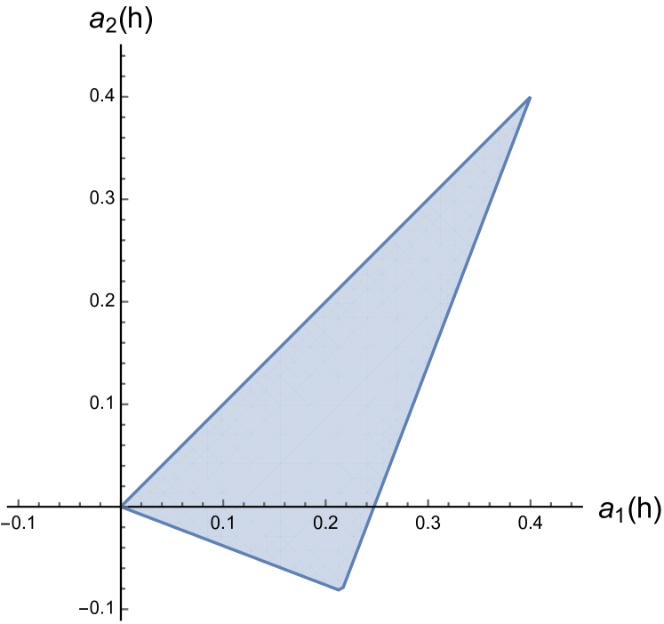
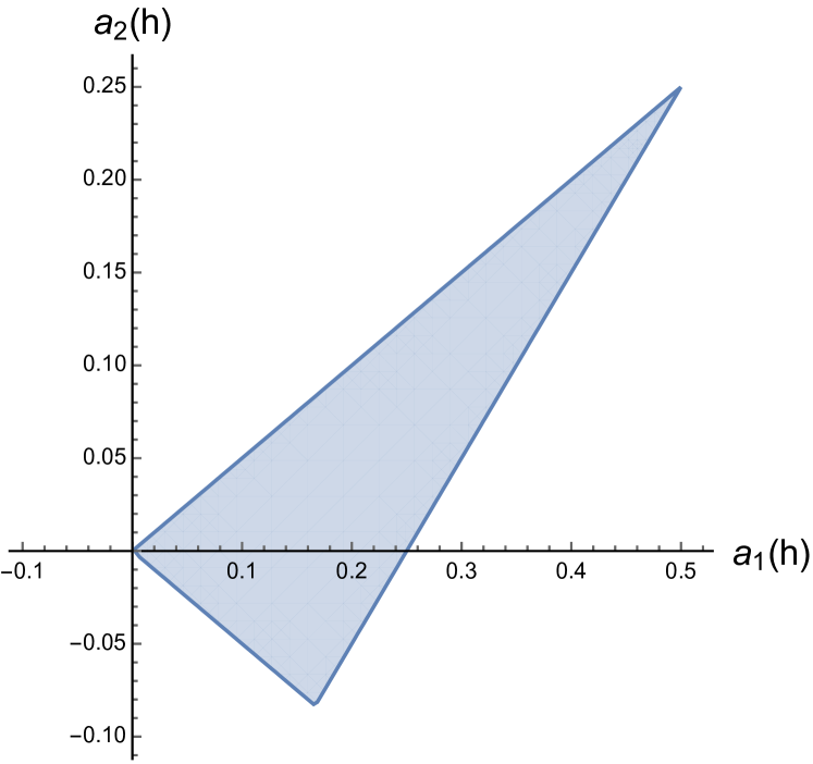
For probability vectors hP+(Ω0)subscript𝑃subscriptΩ0h\in P_{+}(\Omega_{0}) there are of course restrictions on the values of the Fourier modes a1,2subscript𝑎12a_{1,2} that come from 0h(j)10𝑗10\leq h(j)\leq 1 for all jΩ0𝑗subscriptΩ0j\in\Omega_{0} and from the fact that hh is non-increasing. For the region of values the coefficients a1,2subscript𝑎12a_{1,2} can attain in this case, see Figure 1. It can be easily checked that j=0q1h1(j)h2(j)superscriptsubscript𝑗0𝑞1subscript1𝑗subscript2𝑗\sum_{j=0}^{q-1}h_{1}(j)h_{2}(j) is always bounded from below for any choice of h1,h2subscript1subscript2h_{1},h_{2}. Therefore Lemma 3.3 holds for the generalized clock model with q=4,5𝑞45q=4,5 even for transfer matrices with non-positive eigenvalues.
Refer to caption
(a) q=4𝑞4q=4.
Refer to caption
(b) q=5𝑞5q=5.
Figure 1. Region of the coeffcients a1(h),a2(h)subscript𝑎1subscript𝑎2a_{1}(h),a_{2}(h) for a probability vector hP+(Ω0/0)subscript𝑃subscriptΩ00h\in P_{+}(\Omega_{0}/0), where M𝑀M is allowed to have non-positive eigenvalues.

We come to the proof of Proposition 2.5 regarding robust phase transitions on trees in the generalized clock model.

Proof of Proposition 2.5. We will check the necessary conditions for Theorems 3.1 and 3.2 from the paper by Pemantle and Steif [29]:

  1. (i)

    From Lemma 3.3 follows the upper bound for the distance of the convoluted distributions to their linearization.

  2. (ii)

    Note that as P(Ω0/0)𝑃subscriptΩ00P(\Omega_{0}/0) is finite-dimensional all norms are equivalent, in particular the A𝐴A-Norm ||||A||\cdot||_{A} and the supremum norm ||||||\cdot||_{\infty}.

  3. (iii)

    Let ΦΦ\Phi be a potential that corresponds to some circulant transfer matrix M𝑀M. For u(0,1]𝑢01u\in(0,1] we define Musuperscript𝑀𝑢M^{u} to be the transfer matrix that corresponds to the potential uΦ𝑢Φu\Phi, i.e., the first row of Musuperscript𝑀𝑢M^{u} is given by

    ru(j)=exp(uΦ(0,j)).superscript𝑟𝑢𝑗𝑢Φ0𝑗r^{u}(j)=\exp\big{(}-u\Phi(0,j)\big{)}.

    Clearly ru𝟏0subscriptnormsuperscript𝑟𝑢10||r^{u}-\mathbf{1}||_{\infty}\to 0 and hence ru𝟏A0subscriptnormsuperscript𝑟𝑢1𝐴0||r^{u}-\mathbf{1}||_{A}\to 0 for u0𝑢0u\to 0.

  4. (iv)

    The transfer matrix M𝑀M is bounded by 111 in the operator norm:

    MA=supfA=1MfA=supfA=1rfA=supfA=1j=0q/2|aj(rf)|=supfA=1j=0q/2|γjaj(r)aj(f)|=supfA=1j=0q/2|λjaj(f)|supfA=1j=0q/2|aj(f)|=1.subscriptnorm𝑀𝐴subscriptsupremumsubscriptnorm𝑓𝐴1subscriptnorm𝑀𝑓𝐴subscriptsupremumsubscriptnorm𝑓𝐴1subscriptnorm𝑟𝑓𝐴subscriptsupremumsubscriptnorm𝑓𝐴1superscriptsubscript𝑗0𝑞2subscript𝑎𝑗𝑟𝑓subscriptsupremumsubscriptnorm𝑓𝐴1superscriptsubscript𝑗0𝑞2subscript𝛾𝑗subscript𝑎𝑗𝑟subscript𝑎𝑗𝑓subscriptsupremumsubscriptnorm𝑓𝐴1superscriptsubscript𝑗0𝑞2subscript𝜆𝑗subscript𝑎𝑗𝑓subscriptsupremumsubscriptnorm𝑓𝐴1superscriptsubscript𝑗0𝑞2subscript𝑎𝑗𝑓1\begin{split}||M||_{A}&=\sup_{||f||_{A}=1}||Mf||_{A}=\sup_{||f||_{A}=1}||r*f||_{A}\\ &=\sup_{||f||_{A}=1}\sum_{j=0}^{\lfloor q/2\rfloor}|a_{j}(r*f)|=\sup_{||f||_{A}=1}\sum_{j=0}^{\lfloor q/2\rfloor}|\gamma_{j}a_{j}(r)a_{j}(f)|\\ &=\sup_{||f||_{A}=1}\sum_{j=0}^{\lfloor q/2\rfloor}|\lambda_{j}a_{j}(f)|\leq\sup_{||f||_{A}=1}\sum_{j=0}^{\lfloor q/2\rfloor}|a_{j}(f)|=1.\end{split}
  5. (v)

    The next inequality shows that the convolution is in some sense a contraction w.r.t. to the A𝐴A-norm:

    Mf𝟏A=rf𝟏A=j=0q/2|aj(rf𝟏)|=j=0q/2|aj(rf)aj(𝟏)|=j=1q/2|aj(rf)|=j=1q/2|γjaj(r)aj(f)|=j=1q/2|λjaj(f)|λ1j=1q/2|aj(f)|=λ1f𝟏A.subscriptnorm𝑀𝑓1𝐴subscriptnorm𝑟𝑓1𝐴superscriptsubscript𝑗0𝑞2subscript𝑎𝑗𝑟𝑓1superscriptsubscript𝑗0𝑞2subscript𝑎𝑗𝑟𝑓subscript𝑎𝑗1superscriptsubscript𝑗1𝑞2subscript𝑎𝑗𝑟𝑓superscriptsubscript𝑗1𝑞2subscript𝛾𝑗subscript𝑎𝑗𝑟subscript𝑎𝑗𝑓superscriptsubscript𝑗1𝑞2subscript𝜆𝑗subscript𝑎𝑗𝑓subscript𝜆1superscriptsubscript𝑗1𝑞2subscript𝑎𝑗𝑓subscript𝜆1subscriptnorm𝑓1𝐴\begin{split}||Mf-\mathbf{1}||_{A}&=||r*f-\mathbf{1}||_{A}=\sum_{j=0}^{\lfloor q/2\rfloor}|a_{j}(r*f-\mathbf{1})|\\ &=\sum_{j=0}^{\lfloor q/2\rfloor}|a_{j}(r*f)-a_{j}(\mathbf{1})|=\sum_{j=1}^{\lfloor q/2\rfloor}|a_{j}(r*f)|\\ &=\sum_{j=1}^{\lfloor q/2\rfloor}|\gamma_{j}a_{j}(r)a_{j}(f)|=\sum_{j=1}^{\lfloor q/2\rfloor}|\lambda_{j}a_{j}(f)|\\ &\leq\lambda_{1}\sum_{j=1}^{\lfloor q/2\rfloor}|a_{j}(f)|=\lambda_{1}||f-\mathbf{1}||_{A}.\end{split}

Therefore all the conditions for Theorem 3.1 from [29] are met. Hence we can already conclude that in the generalized clock model λ1br(T)<1subscript𝜆1br𝑇1\lambda_{1}\operatorname{br}(T)<1 implies the absence of a RPT.

In the following we check the conditions for Theorem 3.2 of [29]:

  1. (i)

    First we like to note that for all fP+(Ω0/0)𝑓subscript𝑃subscriptΩ00f\in P_{+}(\Omega_{0}/0)

    f(0)=maxkΩ0f(k) and f(q+12)=minkΩ0f(k).formulae-sequence𝑓0subscript𝑘subscriptΩ0𝑓𝑘 and 𝑓𝑞12subscript𝑘subscriptΩ0𝑓𝑘f(0)=\max_{k\in\Omega_{0}}f(k)\quad\mbox{ and }\quad f\Big{(}\left\lceil\frac{q+1}{2}\right\rceil\Big{)}=\min_{k\in\Omega_{0}}f(k).
  2. (ii)

    If f𝑓f is non-increasing, it is easy to see that Mf=rf𝑀𝑓𝑟𝑓Mf=r*f is also non-increasing. Therefore, as a consequence of the recursion (3.1), all fP+(Ω0/0)𝑓subscript𝑃subscriptΩ00f\in P_{+}(\Omega_{0}/0) are non-increasing.
    Define the functional :P(Ω0/0):𝑃subscriptΩ00\mathcal{L}:P(\Omega_{0}/0)\rightarrow\mathbb{R} that captures the weighted absolute value of the first Fourier coefficient by

    (g):=k=0q1g(k)ϕ1(k)=z1a1(g).assign𝑔superscriptsubscript𝑘0𝑞1𝑔𝑘subscriptitalic-ϕ1𝑘subscript𝑧1subscript𝑎1𝑔\mathcal{L}(g):=\sum_{k=0}^{q-1}g(k)\phi_{1}(k)=z_{1}a_{1}(g).

    Let fP+(Ω0/0).𝑓subscript𝑃subscriptΩ00f\in P_{+}(\Omega_{0}/0). Then

    (Mf𝟏)=z1a1(Mf𝟏)=z1a1(rf𝟏)=z1a1(rf)=z12a1(r)a1(f)=(k=0q1r(k)ϕ1(k))(l=0q1f(l)ϕ1(l))=(k=0q1r(k)ϕ1(k))(l=0q1(f(l)𝟏)ϕ1(l))=λ1(f𝟏).𝑀𝑓1subscript𝑧1subscript𝑎1𝑀𝑓1subscript𝑧1subscript𝑎1𝑟𝑓1subscript𝑧1subscript𝑎1𝑟𝑓superscriptsubscript𝑧12subscript𝑎1𝑟subscript𝑎1𝑓superscriptsubscript𝑘0𝑞1𝑟𝑘subscriptitalic-ϕ1𝑘superscriptsubscript𝑙0𝑞1𝑓𝑙subscriptitalic-ϕ1𝑙superscriptsubscript𝑘0𝑞1𝑟𝑘subscriptitalic-ϕ1𝑘superscriptsubscript𝑙0𝑞1𝑓𝑙1subscriptitalic-ϕ1𝑙subscript𝜆1𝑓1\begin{split}\mathcal{L}(Mf-\mathbf{1})&=z_{1}a_{1}(Mf-\mathbf{1})=z_{1}a_{1}(r*f-\mathbf{1})\\ &=z_{1}a_{1}(r*f)=z_{1}^{2}a_{1}(r)a_{1}(f)\\ &=\Big{(}\sum_{k=0}^{q-1}r(k)\phi_{1}(k)\Big{)}\Big{(}\sum_{l=0}^{q-1}f(l)\phi_{1}(l)\Big{)}\\ &=\Big{(}\sum_{k=0}^{q-1}r(k)\phi_{1}(k)\Big{)}\Big{(}\sum_{l=0}^{q-1}(f(l)-\mathbf{1})\phi_{1}(l)\Big{)}=\lambda_{1}\mathcal{L}(f-\mathbf{1}).\end{split}
  3. (iii)

    Note that (f)𝑓\mathcal{L}(f) can be bounded from above by the A𝐴A-norm of f𝑓f:

    |(f)|z1fA𝑓subscript𝑧1subscriptnorm𝑓𝐴|\mathcal{L}(f)|\leq z_{1}||f||_{A}

    for all fP+(Ω0/0).𝑓subscript𝑃subscriptΩ00f\in P_{+}(\Omega_{0}/0).

  4. (iv)

    Now, we want to find a constant d>0𝑑0d>0 s.t. (f)df𝟏A𝑓𝑑subscriptnorm𝑓1𝐴\mathcal{L}(f)\geq d||f-\mathbf{1}||_{A} for all fP+(Ω0/0)𝑓subscript𝑃subscriptΩ00f\in P_{+}(\Omega_{0}/0). We already know that |a1(f)|=a1(f)|aj(f)|subscript𝑎1𝑓subscript𝑎1𝑓subscript𝑎𝑗𝑓|a_{1}(f)|=a_{1}(f)\geq|a_{j}(f)| for all j2𝑗2j\geq 2. Therefore we can choose d:=z1/q2assign𝑑subscript𝑧1𝑞2d:=z_{1}/\left\lfloor\frac{q}{2}\right\rfloor.

Therefore all the prerequisites for Theorem 3.2 in [29] are met as well. Hence we get that in the general clock model λ1brT>1subscript𝜆1br𝑇1\lambda_{1}\operatorname{br}T>1 implies the existence of a RPT and we have finished the proof of Proposition 2.5. \Box

Remark 3.5.

Let us once more consider the q𝑞q-state generalized clock model with q{4,5}𝑞45q\in\{4,5\} on the binary tree. We have already seen in Remark 3.4 that Lemma 3.3 also holds for the case of transition matrices with negative eigenvalues as long as they are non-increasing. One can easily check that all the other prerequisites for Theorem 3.1 from [29] are also met in this case and therefore λ1brT<1subscript𝜆1br𝑇1\lambda_{1}\operatorname{br}T<1 still implies the absence of robust phase transitions.

For the verification of the conditions of Theorem 3.2 from [29] note that the space P+(Ω0/0)subscript𝑃subscriptΩ00P_{+}(\Omega_{0}/0) is three-dimensional and |a1(f)|=a1(f)|a2(f)|subscript𝑎1𝑓subscript𝑎1𝑓subscript𝑎2𝑓|a_{1}(f)|=a_{1}(f)\geq|a_{2}(f)| for every fP+(Ω0/0)𝑓subscript𝑃subscriptΩ00f\in P_{+}(\Omega_{0}/0). It is then easily seen that for suitably chosen constant c4subscript𝑐4c_{4} indeed L(f)c4f1A𝐿𝑓subscript𝑐4subscriptnorm𝑓1𝐴L(f)\geq c_{4}||f-1||_{A} for all fP+(Ω0/0)𝑓subscript𝑃subscriptΩ00f\in P_{+}(\Omega_{0}/0). For q=4,5𝑞45q=4,5 the constant can be chosen to be c4=2/z1subscript𝑐42subscript𝑧1c_{4}=2/z_{1}. All the other conditions of Theorem 3.2 are clearly met as well.

We conclude that for q=4,5𝑞45q=4,5 the sharp threshold for the existence of a RPT holds even for transition matrices with negative eigenvalues as long as the transfer matrix M𝑀M is non-increasing.

4. Non-robust phase transitions in the generalized clock model on the binary tree

4.1. Case q=5

In this section we will take a closer look at the generalized clock model with local state space Ω0={0,,4}subscriptΩ004\Omega_{0}=\{0,...,4\}. Furthermore we will assume that T𝑇T is the binary tree, i.e., the Cayley tree 𝒞𝒯(2)𝒞𝒯2\mathcal{C}\mathcal{T}(2). The first row of the transfer matrix M𝑀M is given by

r=(r0,r1,r2,r3,r4)=(a,b,c,c,b),𝑟subscript𝑟0subscript𝑟1subscript𝑟2subscript𝑟3subscript𝑟4𝑎𝑏𝑐𝑐𝑏r=(r_{0},r_{1},r_{2},r_{3},r_{4})=(a,b,c,c,b),

where a+2b+2c=1𝑎2𝑏2𝑐1a+2b+2c=1. As M𝑀M is symmetric there are five eigenvalues λi,i=0,,4formulae-sequencesubscript𝜆𝑖𝑖04\lambda_{i},i=0,...,4, that are given by

λm=k=04rkexp(2πimk/5).subscript𝜆𝑚superscriptsubscript𝑘04subscript𝑟𝑘2𝜋𝑖𝑚𝑘5\lambda_{m}=\sum_{k=0}^{4}r_{k}\exp\big{(}-2\pi imk/5\big{)}.

This gives us

λ0=1,λ1=a+2bcos(2π/5)+2ccos(4π/5)=λ4formulae-sequencesubscript𝜆01subscript𝜆1𝑎2𝑏2𝜋52𝑐4𝜋5subscript𝜆4\lambda_{0}=1,\quad\lambda_{1}=a+2b\cos(2\pi/5)+2c\cos(4\pi/5)=\lambda_{4}

and

λ2=a+2bcos(4π/5)+2ccos(2π/5)=λ3.subscript𝜆2𝑎2𝑏4𝜋52𝑐2𝜋5subscript𝜆3\lambda_{2}=a+2b\cos(4\pi/5)+2c\cos(2\pi/5)=\lambda_{3}.

In the following we will assume that λ112subscript𝜆112\lambda_{1}\leq\frac{1}{2} and 1=λ0>λ1λ21subscript𝜆0subscript𝜆1subscript𝜆21=\lambda_{0}>\lambda_{1}\geq\lambda_{2} are given in such a way that M𝑀M is non-increasing. The assumption λ112subscript𝜆112\lambda_{1}\leq\frac{1}{2} is made as this is the known critical value for the existence of a robust phase transition in the generalized clock model on the binary tree. The inequality λ1λ2subscript𝜆1subscript𝜆2\lambda_{1}\geq\lambda_{2} is necessary for M𝑀M being non-increasing. By the Fourier inversion formula the eigenvalues determine the first row of M𝑀M. We have

rl=15m=04λmexp(2πilm/5)subscript𝑟𝑙15superscriptsubscript𝑚04subscript𝜆𝑚2𝜋𝑖𝑙𝑚5r_{l}=\frac{1}{5}\sum_{m=0}^{4}\lambda_{m}\exp\big{(}2\pi ilm/5\big{)}

and therefore

r0=15(1+2λ1+2λ2),r1=15(1+2λ1cos(2π/5)+2λ2cos(4π/5))=r4,r2=15(1+2λ1cos(4π/5)+2λ2cos(2π/5))=r3.formulae-sequenceformulae-sequencesubscript𝑟01512subscript𝜆12subscript𝜆2subscript𝑟11512subscript𝜆12𝜋52subscript𝜆24𝜋5subscript𝑟4subscript𝑟21512subscript𝜆14𝜋52subscript𝜆22𝜋5subscript𝑟3\begin{split}r_{0}&=\frac{1}{5}(1+2\lambda_{1}+2\lambda_{2}),\\ r_{1}&=\frac{1}{5}(1+2\lambda_{1}\cos(2\pi/5)+2\lambda_{2}\cos(4\pi/5))=r_{4},\\ r_{2}&=\frac{1}{5}(1+2\lambda_{1}\cos(4\pi/5)+2\lambda_{2}\cos(2\pi/5))=r_{3}.\end{split}

The recursion for the marginal distributions of the Gibbs measure can now be seen as acting on the orthogonal space of the constant function, that is the set of symmetric mass zero measures, {pP(Ω0/0)k=0q1pk=0}conditional-set𝑝𝑃subscriptΩ00superscriptsubscript𝑘0𝑞1subscript𝑝𝑘0\{p\in P(\Omega_{0}/0)\mid\sum_{k=0}^{q-1}p_{k}=0\}. For q=5𝑞5q=5 this space is two-dimensional with basis {ϕ1,ϕ2}subscriptitalic-ϕ1subscriptitalic-ϕ2\{\phi_{1},\phi_{2}\}, where

ϕ1:=c1(1,cos(2π/5),cos(4π/5),cos(4π/5),cos(2π/5))Tassignsubscriptitalic-ϕ1superscript𝑐1superscript12𝜋54𝜋54𝜋52𝜋5𝑇\phi_{1}:=c^{-1}(1,\cos(2\pi/5),\cos(4\pi/5),\cos(4\pi/5),\cos(2\pi/5))^{T}

and

ϕ2:=c1(1,cos(4π/5),cos(2π/5),cos(2π/5),cos(4π/5))Tassignsubscriptitalic-ϕ2superscript𝑐1superscript14𝜋52𝜋52𝜋54𝜋5𝑇\phi_{2}:=c^{-1}(1,\cos(4\pi/5),\cos(2\pi/5),\cos(2\pi/5),\cos(4\pi/5))^{T}

with

c:=1+2cos2(2π/5)+2cos2(4π/5)assign𝑐12superscript22𝜋52superscript24𝜋5c:=\sqrt{1+2\cos^{2}(2\pi/5)+2\cos^{2}(4\pi/5)}

being a normalizing constant. For a probability distribution α1(Ω0)𝛼subscript1subscriptΩ0\alpha\in\mathcal{M}_{1}(\Omega_{0}) given by

α(j)=1q+k=12αkϕk(j),𝛼𝑗1𝑞superscriptsubscript𝑘12subscript𝛼𝑘subscriptitalic-ϕ𝑘𝑗\alpha(j)=\frac{1}{q}+\sum_{k=1}^{2}\alpha_{k}\phi_{k}(j),

with αksubscript𝛼𝑘\alpha_{k} being the Fourier coefficients, we have

Mα(j)=1q+k=12λkαkϕk(j).𝑀𝛼𝑗1𝑞superscriptsubscript𝑘12subscript𝜆𝑘subscript𝛼𝑘subscriptitalic-ϕ𝑘𝑗M\alpha(j)=\frac{1}{q}+\sum_{k=1}^{2}\lambda_{k}\alpha_{k}\phi_{k}(j).

Let F5subscript𝐹5F_{5} be the non-linear map which represents the recursion. As we are operating on the binary tree, recursion equation (3.1) boils down to

α(j)=F5α(j):=(1q+k=12λkαkϕk(j))2j=04(1q+k=12λkαkϕk(j))2.𝛼𝑗subscript𝐹5𝛼𝑗assignsuperscript1𝑞superscriptsubscript𝑘12subscript𝜆𝑘subscript𝛼𝑘subscriptitalic-ϕ𝑘𝑗2superscriptsubscript𝑗04superscript1𝑞superscriptsubscript𝑘12subscript𝜆𝑘subscript𝛼𝑘subscriptitalic-ϕ𝑘𝑗2\alpha(j)=F_{5}\alpha(j):=\frac{\left(\frac{1}{q}+\sum_{k=1}^{2}\lambda_{k}\alpha_{k}\phi_{k}(j)\right)^{2}}{\sum_{j=0}^{4}\left(\frac{1}{q}+\sum_{k=1}^{2}\lambda_{k}\alpha_{k}\phi_{k}(j)\right)^{2}}.

For the summands in the numerator we have

(Mα(j))2=1q2+2qk=12λkαkϕk(j)+k=12l=12αkαlλkλlϕk(j)ϕl(j).superscript𝑀𝛼𝑗21superscript𝑞22𝑞superscriptsubscript𝑘12subscript𝜆𝑘subscript𝛼𝑘subscriptitalic-ϕ𝑘𝑗superscriptsubscript𝑘12superscriptsubscript𝑙12subscript𝛼𝑘subscript𝛼𝑙subscript𝜆𝑘subscript𝜆𝑙subscriptitalic-ϕ𝑘𝑗subscriptitalic-ϕ𝑙𝑗(M\alpha(j))^{2}=\frac{1}{q^{2}}+\frac{2}{q}\sum_{k=1}^{2}\lambda_{k}\alpha_{k}\phi_{k}(j)+\sum_{k=1}^{2}\sum_{l=1}^{2}\alpha_{k}\alpha_{l}\lambda_{k}\lambda_{l}\phi_{k}(j)\phi_{l}(j).

By the addition theorem for the cosine follows

ϕk(j)ϕl(j)=v(ϕk+l(j)+ϕkl(j))subscriptitalic-ϕ𝑘𝑗subscriptitalic-ϕ𝑙𝑗𝑣subscriptitalic-ϕ𝑘𝑙𝑗subscriptitalic-ϕ𝑘𝑙𝑗\phi_{k}(j)\phi_{l}(j)=v(\phi_{k+l}(j)+\phi_{k-l}(j))

and

ϕk(j)2=vϕ2k(j)+w,subscriptitalic-ϕ𝑘superscript𝑗2𝑣subscriptitalic-ϕ2𝑘𝑗𝑤\phi_{k}(j)^{2}=v\phi_{2k}(j)+w,

where v:=12cassign𝑣12𝑐v:=\frac{1}{2c} and w:=12c2=2v2=1qassign𝑤12superscript𝑐22superscript𝑣21𝑞w:=\frac{1}{2c^{2}}=2v^{2}=\frac{1}{q}. This gives us

(Mα(j))2=1q2+2qk=12λkαkϕk(j)+v1k,l2,klαkαlλkλl(ϕk+l(j)+ϕkl(j))+v1k2αk2λk2ϕ2k(j)+w1k2αk2λk2superscript𝑀𝛼𝑗21superscript𝑞22𝑞superscriptsubscript𝑘12subscript𝜆𝑘subscript𝛼𝑘subscriptitalic-ϕ𝑘𝑗𝑣subscriptformulae-sequence1𝑘formulae-sequence𝑙2𝑘𝑙subscript𝛼𝑘subscript𝛼𝑙subscript𝜆𝑘subscript𝜆𝑙subscriptitalic-ϕ𝑘𝑙𝑗subscriptitalic-ϕ𝑘𝑙𝑗𝑣subscript1𝑘2subscriptsuperscript𝛼2𝑘superscriptsubscript𝜆𝑘2subscriptitalic-ϕ2𝑘𝑗𝑤subscript1𝑘2subscriptsuperscript𝛼2𝑘subscriptsuperscript𝜆2𝑘\begin{split}(M\alpha(j))^{2}&=\frac{1}{q^{2}}+\frac{2}{q}\sum_{k=1}^{2}\lambda_{k}\alpha_{k}\phi_{k}(j)+v\sum_{1\leq k,l\leq 2,k\neq l}\alpha_{k}\alpha_{l}\lambda_{k}\lambda_{l}(\phi_{k+l}(j)+\phi_{k-l}(j))\\ &\qquad+v\sum_{1\leq k\leq 2}\alpha^{2}_{k}\lambda_{k}^{2}\phi_{2k}(j)+w\sum_{1\leq k\leq 2}\alpha^{2}_{k}\lambda^{2}_{k}\cr\end{split}

and by orthogonality of the basis functions ϕ1,ϕ2subscriptitalic-ϕ1subscriptitalic-ϕ2\phi_{1},\phi_{2} the normalization is just

1jq(Mα(j))2=1q+wq1k2αk2λk2.subscript1𝑗𝑞superscript𝑀𝛼𝑗21𝑞𝑤𝑞subscript1𝑘2subscriptsuperscript𝛼2𝑘subscriptsuperscript𝜆2𝑘\begin{split}&\sum_{1\leq j\leq q}(M\alpha(j))^{2}=\frac{1}{q}+wq\sum_{1\leq k\leq 2}\alpha^{2}_{k}\lambda^{2}_{k}.\end{split}

Therefore the recursion can be written as

(4.1) F5α(j)=1q+11q+wq1k2αk2λk2(2qk=12λkαkϕk(j)+v1k,l2,klαkαlλkλl(ϕk+l(j)+ϕkl(j))+v1k2αk2λk2ϕ2k(j))=1q+m=12αmϕm(j).subscript𝐹5𝛼𝑗1𝑞11𝑞𝑤𝑞subscript1𝑘2subscriptsuperscript𝛼2𝑘subscriptsuperscript𝜆2𝑘2𝑞superscriptsubscript𝑘12subscript𝜆𝑘subscript𝛼𝑘subscriptitalic-ϕ𝑘𝑗𝑣subscriptformulae-sequence1𝑘formulae-sequence𝑙2𝑘𝑙subscript𝛼𝑘subscript𝛼𝑙subscript𝜆𝑘subscript𝜆𝑙subscriptitalic-ϕ𝑘𝑙𝑗subscriptitalic-ϕ𝑘𝑙𝑗𝑣subscript1𝑘2subscriptsuperscript𝛼2𝑘superscriptsubscript𝜆𝑘2subscriptitalic-ϕ2𝑘𝑗1𝑞superscriptsubscript𝑚12subscriptsuperscript𝛼𝑚subscriptitalic-ϕ𝑚𝑗\begin{split}F_{5}\alpha(j)&=\frac{1}{q}+\frac{1}{\frac{1}{q}+wq\sum_{1\leq k\leq 2}\alpha^{2}_{k}\lambda^{2}_{k}}\Bigl{(}\frac{2}{q}\sum_{k=1}^{2}\lambda_{k}\alpha_{k}\phi_{k}(j)\\ +&\quad v\sum_{1\leq k,l\leq 2,k\neq l}\alpha_{k}\alpha_{l}\lambda_{k}\lambda_{l}(\phi_{k+l}(j)+\phi_{k-l}(j))+v\sum_{1\leq k\leq 2}\alpha^{2}_{k}\lambda_{k}^{2}\phi_{2k}(j)\Bigr{)}\cr&=\frac{1}{q}+\sum_{m=1}^{2}\alpha^{\prime}_{m}\phi_{m}(j).\end{split}

For q=5𝑞5q=5 this gives

11q+wq1k2αk2λk2(2qk=12λkαkϕk(j)+1k,l2,klαkαlλkλlv(ϕk+l(j)+ϕkl(j))+v1k2αk2λk2ϕ2k(j))=m=12αmϕm(j).11𝑞𝑤𝑞subscript1𝑘2subscriptsuperscript𝛼2𝑘subscriptsuperscript𝜆2𝑘2𝑞superscriptsubscript𝑘12subscript𝜆𝑘subscript𝛼𝑘subscriptitalic-ϕ𝑘𝑗subscriptformulae-sequence1𝑘formulae-sequence𝑙2𝑘𝑙subscript𝛼𝑘subscript𝛼𝑙subscript𝜆𝑘subscript𝜆𝑙𝑣subscriptitalic-ϕ𝑘𝑙𝑗subscriptitalic-ϕ𝑘𝑙𝑗𝑣subscript1𝑘2subscriptsuperscript𝛼2𝑘superscriptsubscript𝜆𝑘2subscriptitalic-ϕ2𝑘𝑗superscriptsubscript𝑚12subscriptsuperscript𝛼𝑚subscriptitalic-ϕ𝑚𝑗\begin{split}&\frac{1}{\frac{1}{q}+wq\sum_{1\leq k\leq 2}\alpha^{2}_{k}\lambda^{2}_{k}}\Bigl{(}\frac{2}{q}\sum_{k=1}^{2}\lambda_{k}\alpha_{k}\phi_{k}(j)\cr&+\sum_{1\leq k,l\leq 2,k\neq l}\alpha_{k}\alpha_{l}\lambda_{k}\lambda_{l}v(\phi_{k+l}(j)+\phi_{k-l}(j))+v\sum_{1\leq k\leq 2}\alpha^{2}_{k}\lambda_{k}^{2}\phi_{2k}(j)\Bigr{)}\cr&=\sum_{m=1}^{2}\alpha^{\prime}_{m}\phi_{m}(j).\end{split}

Rewriting these last equations produces two fixed-point equations for the Fourier modes α1subscript𝛼1\alpha_{1} and α2subscript𝛼2\alpha_{2}:

(4.2) α1=115+α12λ12+α22λ22(25λ1α1+2λ1λ2vα1α2+vλ22α22)subscript𝛼1115superscriptsubscript𝛼12superscriptsubscript𝜆12superscriptsubscript𝛼22superscriptsubscript𝜆2225subscript𝜆1subscript𝛼12subscript𝜆1subscript𝜆2𝑣subscript𝛼1subscript𝛼2𝑣superscriptsubscript𝜆22superscriptsubscript𝛼22\alpha_{1}=\frac{1}{\frac{1}{5}+\alpha_{1}^{2}\lambda_{1}^{2}+\alpha_{2}^{2}\lambda_{2}^{2}}\left(\frac{2}{5}\lambda_{1}\alpha_{1}+2\lambda_{1}\lambda_{2}v\alpha_{1}\alpha_{2}+v\lambda_{2}^{2}\alpha_{2}^{2}\right)

and

(4.3) α2=115+α12λ12+α22λ22(25λ2α2+2λ1λ2vα1α2+vλ12α12).subscript𝛼2115superscriptsubscript𝛼12superscriptsubscript𝜆12superscriptsubscript𝛼22superscriptsubscript𝜆2225subscript𝜆2subscript𝛼22subscript𝜆1subscript𝜆2𝑣subscript𝛼1subscript𝛼2𝑣superscriptsubscript𝜆12superscriptsubscript𝛼12\alpha_{2}=\frac{1}{\frac{1}{5}+\alpha_{1}^{2}\lambda_{1}^{2}+\alpha_{2}^{2}\lambda_{2}^{2}}\left(\frac{2}{5}\lambda_{2}\alpha_{2}+2\lambda_{1}\lambda_{2}v\alpha_{1}\alpha_{2}+v\lambda_{1}^{2}\alpha_{1}^{2}\right).

We set λ1=12subscript𝜆112\lambda_{1}=\frac{1}{2} as this is the critical value for the existence of RPT on the binary tree. Note that α1=0subscript𝛼10\alpha_{1}=0 if and only if α2=0subscript𝛼20\alpha_{2}=0. We define

A:=20λ22α22.assign𝐴20superscriptsubscript𝜆22superscriptsubscript𝛼22A:=20\lambda_{2}^{2}\alpha_{2}^{2}.

From the first of these equations we get

α1(4+5α12+A)=4α1+20λ2vα1α2+vAsubscript𝛼145superscriptsubscript𝛼12𝐴4subscript𝛼120subscript𝜆2𝑣subscript𝛼1subscript𝛼2𝑣𝐴\begin{split}\alpha_{1}(4+5\alpha_{1}^{2}+A)&=4\alpha_{1}+20\lambda_{2}v\alpha_{1}\alpha_{2}+vA\end{split}

and hence

(4.4) A=20λ2vα1α25α13α1v𝐴20subscript𝜆2𝑣subscript𝛼1subscript𝛼25superscriptsubscript𝛼13subscript𝛼1𝑣A=\frac{20\lambda_{2}v\alpha_{1}\alpha_{2}-5\alpha_{1}^{3}}{\alpha_{1}-v}

for α1vsubscript𝛼1𝑣\alpha_{1}\neq v. In the case where α1=vsubscript𝛼1𝑣\alpha_{1}=v we find α2=v4λ2subscript𝛼2𝑣4subscript𝜆2\alpha_{2}=\frac{v}{4\lambda_{2}}. Plugging these values into the second fixed-point equation shows that this solution only appears for λ2=(15v+14v3+116v3)/(25v+2v3)0.385417subscript𝜆215𝑣14superscript𝑣3116superscript𝑣325𝑣2superscript𝑣30.385417\lambda_{2}=(\frac{1}{5}v+\frac{1}{4}v^{3}+\frac{1}{16}v^{3})/(\frac{2}{5}v+2v^{3})\approx 0.385417.

Continuing with the second equation for α1vsubscript𝛼1𝑣\alpha_{1}\neq v we may use (4.4) to reduce the order of α2subscript𝛼2\alpha_{2} repeatedly. This leads to

α2=8λ2α2+20λ2vα1α2+5vα124+5α12+20λ2vα1α25α13α1vα2(4α1+5α134v5vα12+20λ2vα1α25α13)=(α1v)(8λ2α2+20λ2vα1α2+5vα12)4α2(α1v)5vα12α2+vα1λ2(20λ2vα1α25α13α1v)=(α1v)(8λ2α2+20λ2vα1α2+5vα12)(4λ2(α1v)25λ2vα12(α1v)+20λ2v2α128λ22(α1v)220λ22vα1(α1v)2)α2=5vα14+5vλ2α12(α1v)2.subscript𝛼28subscript𝜆2subscript𝛼220subscript𝜆2𝑣subscript𝛼1subscript𝛼25𝑣superscriptsubscript𝛼1245superscriptsubscript𝛼1220subscript𝜆2𝑣subscript𝛼1subscript𝛼25superscriptsubscript𝛼13subscript𝛼1𝑣subscript𝛼24subscript𝛼15superscriptsubscript𝛼134𝑣5𝑣superscriptsubscript𝛼1220subscript𝜆2𝑣subscript𝛼1subscript𝛼25superscriptsubscript𝛼13subscript𝛼1𝑣8subscript𝜆2subscript𝛼220subscript𝜆2𝑣subscript𝛼1subscript𝛼25𝑣superscriptsubscript𝛼124subscript𝛼2subscript𝛼1𝑣5𝑣superscriptsubscript𝛼12subscript𝛼2𝑣subscript𝛼1subscript𝜆220subscript𝜆2𝑣subscript𝛼1subscript𝛼25superscriptsubscript𝛼13subscript𝛼1𝑣subscript𝛼1𝑣8subscript𝜆2subscript𝛼220subscript𝜆2𝑣subscript𝛼1subscript𝛼25𝑣superscriptsubscript𝛼124subscript𝜆2superscriptsubscript𝛼1𝑣25subscript𝜆2𝑣superscriptsubscript𝛼12subscript𝛼1𝑣20subscript𝜆2superscript𝑣2superscriptsubscript𝛼128superscriptsubscript𝜆22superscriptsubscript𝛼1𝑣220superscriptsubscript𝜆22𝑣subscript𝛼1superscriptsubscript𝛼1𝑣2subscript𝛼25𝑣superscriptsubscript𝛼145𝑣subscript𝜆2superscriptsubscript𝛼12superscriptsubscript𝛼1𝑣2\begin{split}&\alpha_{2}=\frac{8\lambda_{2}\alpha_{2}+20\lambda_{2}v\alpha_{1}\alpha_{2}+5v\alpha_{1}^{2}}{4+5\alpha_{1}^{2}+\frac{20\lambda_{2}v\alpha_{1}\alpha_{2}-5\alpha_{1}^{3}}{\alpha_{1}-v}}\\ \implies&\alpha_{2}\Big{(}4\alpha_{1}+5\alpha_{1}^{3}-4v-5v\alpha_{1}^{2}+20\lambda_{2}v\alpha_{1}\alpha_{2}-5\alpha_{1}^{3}\Big{)}\\ &\qquad=(\alpha_{1}-v)(8\lambda_{2}\alpha_{2}+20\lambda_{2}v\alpha_{1}\alpha_{2}+5v\alpha_{1}^{2})\\ \implies&4\alpha_{2}(\alpha_{1}-v)-5v\alpha_{1}^{2}\alpha_{2}+\frac{v\alpha_{1}}{\lambda_{2}}\Big{(}\frac{20\lambda_{2}v\alpha_{1}\alpha_{2}-5\alpha_{1}^{3}}{\alpha_{1}-v}\Big{)}\\ &\qquad=(\alpha_{1}-v)(8\lambda_{2}\alpha_{2}+20\lambda_{2}v\alpha_{1}\alpha_{2}+5v\alpha_{1}^{2})\\ \implies&\Big{(}4\lambda_{2}(\alpha_{1}-v)^{2}-5\lambda_{2}v\alpha_{1}^{2}(\alpha_{1}-v)+20\lambda_{2}v^{2}\alpha_{1}^{2}-8\lambda_{2}^{2}(\alpha_{1}-v)^{2}\\ &\qquad-20\lambda_{2}^{2}v\alpha_{1}(\alpha_{1}-v)^{2}\Big{)}\alpha_{2}=5v\alpha_{1}^{4}+5v\lambda_{2}\alpha_{1}^{2}(\alpha_{1}-v)^{2}.\end{split}

For P3(α1)0subscript𝑃3subscript𝛼10P_{3}(\alpha_{1})\neq 0 we have

(4.5) α2=f(α1)=P4(α1)P3(α1),subscript𝛼2𝑓subscript𝛼1subscript𝑃4subscript𝛼1subscript𝑃3subscript𝛼1\begin{split}\alpha_{2}=f(\alpha_{1})=\frac{P_{4}(\alpha_{1})}{P_{3}(\alpha_{1})},\end{split}

where

P3(α1)=4λ2(α1v)25λ2vα12(α1v)+20λ2v2α128λ22(α1v)220λ22vα1(α1v)2subscript𝑃3subscript𝛼14subscript𝜆2superscriptsubscript𝛼1𝑣25subscript𝜆2𝑣superscriptsubscript𝛼12subscript𝛼1𝑣20subscript𝜆2superscript𝑣2superscriptsubscript𝛼128superscriptsubscript𝜆22superscriptsubscript𝛼1𝑣220superscriptsubscript𝜆22𝑣subscript𝛼1superscriptsubscript𝛼1𝑣2\begin{split}P_{3}(\alpha_{1})&=4\lambda_{2}(\alpha_{1}-v)^{2}-5\lambda_{2}v\alpha_{1}^{2}(\alpha_{1}-v)+20\lambda_{2}v^{2}\alpha_{1}^{2}\\ &\qquad-8\lambda_{2}^{2}(\alpha_{1}-v)^{2}-20\lambda_{2}^{2}v\alpha_{1}(\alpha_{1}-v)^{2}\end{split}

and

P4(α1)=5vα14+5vλ2α12(α1v)2.subscript𝑃4subscript𝛼15𝑣superscriptsubscript𝛼145𝑣subscript𝜆2superscriptsubscript𝛼12superscriptsubscript𝛼1𝑣2P_{4}(\alpha_{1})=5v\alpha_{1}^{4}+5v\lambda_{2}\alpha_{1}^{2}(\alpha_{1}-v)^{2}.

If P3(α1)=0subscript𝑃3subscript𝛼10P_{3}(\alpha_{1})=0 there is only the trivial solution. Substituting (4.5) for the first fixed-point equation leaves us to solve

5α13P32(α1)+20λ22P42(α1)α120λ2vα1P3(α1)P4(α1)20vλ22P42(α1)=0,5superscriptsubscript𝛼13superscriptsubscript𝑃32subscript𝛼120superscriptsubscript𝜆22superscriptsubscript𝑃42subscript𝛼1subscript𝛼120subscript𝜆2𝑣subscript𝛼1subscript𝑃3subscript𝛼1subscript𝑃4subscript𝛼120𝑣superscriptsubscript𝜆22superscriptsubscript𝑃42subscript𝛼105\alpha_{1}^{3}P_{3}^{2}(\alpha_{1})+20\lambda_{2}^{2}P_{4}^{2}(\alpha_{1})\alpha_{1}-20\lambda_{2}v\alpha_{1}P_{3}(\alpha_{1})P_{4}(\alpha_{1})-20v\lambda_{2}^{2}P_{4}^{2}(\alpha_{1})=0,

which is equivalent to

(4.6) α13(α1v)2[α14(125λ222+200λ23+250λ24)+α13(2010λ227510λ23+12510λ24)+α12(140λ22345λ23+75λ24)+α1(1610λ22+6410λ2312552λ24)+8λ2236λ23+40λ24]=:α13(α1v)2qλ2(α1).\begin{split}\alpha_{1}^{3}(\alpha_{1}-v)^{2}\Big{[}&\alpha_{1}^{4}\left(\frac{125\lambda_{2}^{2}}{2}+200\lambda_{2}^{3}+250\lambda_{2}^{4}\right)\\ &+\alpha_{1}^{3}\left(-20\sqrt{10}\lambda_{2}^{2}-75\sqrt{10}\lambda_{2}^{3}+125\sqrt{10}\lambda_{2}^{4}\right)\\ &+\alpha_{1}^{2}\left(140\lambda_{2}^{2}-345\lambda_{2}^{3}+75\lambda_{2}^{4}\right)\\ &+\alpha_{1}\left(-16\sqrt{10}\lambda_{2}^{2}+64\sqrt{10}\lambda_{2}^{3}-125\sqrt{\frac{5}{2}}\lambda_{2}^{4}\right)\\ &+8\lambda_{2}^{2}-36\lambda_{2}^{3}+40\lambda_{2}^{4}\Big{]}=:\alpha_{1}^{3}(\alpha_{1}-v)^{2}q_{\lambda_{2}}(\alpha_{1}).\end{split}

Let us write for the quartic function qλ2(α1)=aα14+bα13+cα12+dα1+esubscript𝑞subscript𝜆2subscript𝛼1𝑎superscriptsubscript𝛼14𝑏superscriptsubscript𝛼13𝑐superscriptsubscript𝛼12𝑑subscript𝛼1𝑒q_{\lambda_{2}}(\alpha_{1})=a\alpha_{1}^{4}+b\alpha_{1}^{3}+c\alpha_{1}^{2}+d\alpha_{1}+e. Looking at the discriminant ΔΔ\Delta of qλ2subscript𝑞subscript𝜆2q_{\lambda_{2}}, i.e.,

Δ=256a3e3192a2bde2128a2c2e2+144a2cd2e27a2d4+144ab2ce26ab2d2e80abc2de+18abcd3+16ac4e4ac3d227b4e2+18b3cde4b3d34b2c3e+b2c2d2,Δ256superscript𝑎3superscript𝑒3192superscript𝑎2𝑏𝑑superscript𝑒2128superscript𝑎2superscript𝑐2superscript𝑒2144superscript𝑎2𝑐superscript𝑑2𝑒27superscript𝑎2superscript𝑑4144𝑎superscript𝑏2𝑐superscript𝑒26𝑎superscript𝑏2superscript𝑑2𝑒80𝑎𝑏superscript𝑐2𝑑𝑒18𝑎𝑏𝑐superscript𝑑316𝑎superscript𝑐4𝑒4𝑎superscript𝑐3superscript𝑑227superscript𝑏4superscript𝑒218superscript𝑏3𝑐𝑑𝑒4superscript𝑏3superscript𝑑34superscript𝑏2superscript𝑐3𝑒superscript𝑏2superscript𝑐2superscript𝑑2\begin{split}\Delta&=256a^{3}e^{3}-192a^{2}bde^{2}-128a^{2}c^{2}e^{2}+144a^{2}cd^{2}e-27a^{2}d^{4}\\ &\quad+144ab^{2}ce^{2}-6ab^{2}d^{2}e-80abc^{2}de+18abcd^{3}+16ac^{4}e\\ &\quad-4ac^{3}d^{2}-27b^{4}e^{2}+18b^{3}cde-4b^{3}d^{3}-4b^{2}c^{3}e+b^{2}c^{2}d^{2},\end{split}

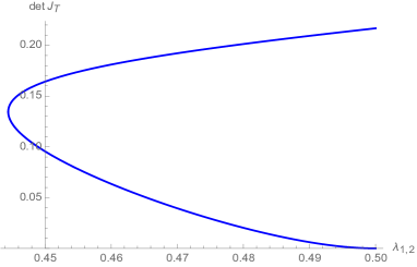
it can be shown by numerical calculations that there exists no non-trivial solutions for α1subscript𝛼1\alpha_{1} if 0λ2<λ2c0subscript𝜆2superscriptsubscript𝜆2𝑐0\leq\lambda_{2}<\lambda_{2}^{c}, where λ2csuperscriptsubscript𝜆2𝑐\lambda_{2}^{c} is a real root of ΔΔ\Delta with λ2c0.370748superscriptsubscript𝜆2𝑐0.370748\lambda_{2}^{c}\approx 0.370748. Indeed, in this regime we have Δ(λ2)>0Δsubscript𝜆20\Delta(\lambda_{2})>0 and P(λ2)>0𝑃subscript𝜆20P(\lambda_{2})>0, where

P:=8ac3b2.assign𝑃8𝑎𝑐3superscript𝑏2P:=8ac-3b^{2}.

This is a well-known sufficient condition for the non-existence of any real roots of the quartic function qλ2subscript𝑞subscript𝜆2q_{\lambda_{2}}. For the critical value λ2csuperscriptsubscript𝜆2𝑐\lambda_{2}^{c} we have that Δ(λ2c)=0,P(λ2c)>0formulae-sequenceΔsuperscriptsubscript𝜆2𝑐0𝑃superscriptsubscript𝜆2𝑐0\Delta(\lambda_{2}^{c})=0,P(\lambda_{2}^{c})>0 and D(λ2c)0𝐷superscriptsubscript𝜆2𝑐0D(\lambda_{2}^{c})\neq 0, where

D:=64a3e16a2c2+16ab2c16a2bd3b4.assign𝐷64superscript𝑎3𝑒16superscript𝑎2superscript𝑐216𝑎superscript𝑏2𝑐16superscript𝑎2𝑏𝑑3superscript𝑏4D:=64a^{3}e-16a^{2}c^{2}+16ab^{2}c-16a^{2}bd-3b^{4}.

This means that for λ2=λ2csubscript𝜆2superscriptsubscript𝜆2𝑐\lambda_{2}=\lambda_{2}^{c} a double real root for qλ2subscript𝑞subscript𝜆2q_{\lambda_{2}} appears. For λ2(λ2c,λ~2c)subscript𝜆2superscriptsubscript𝜆2𝑐superscriptsubscript~𝜆2𝑐\lambda_{2}\in(\lambda_{2}^{c},\tilde{\lambda}_{2}^{c}) where Δ(λ~2c)=0Δsuperscriptsubscript~𝜆2𝑐0\Delta(\tilde{\lambda}_{2}^{c})=0 with λ~2c0.494119superscriptsubscript~𝜆2𝑐0.494119\tilde{\lambda}_{2}^{c}\approx 0.494119 we see by numerical computations that Δ(λ2)<0Δsubscript𝜆20\Delta(\lambda_{2})<0 and hence there exist exactly two distinct real roots for qλ2subscript𝑞subscript𝜆2q_{\lambda_{2}}. In the regime where λ2>λ~2csubscript𝜆2superscriptsubscript~𝜆2𝑐\lambda_{2}>\tilde{\lambda}_{2}^{c} we have that Δ(λ2)>0Δsubscript𝜆20\Delta(\lambda_{2})>0, P(λ2)<0𝑃subscript𝜆20P(\lambda_{2})<0 and D(λ2)<0𝐷subscript𝜆20D(\lambda_{2})<0. Hence there exist four distinct real roots in this case. In the situation where λ2=λ~2csubscript𝜆2superscriptsubscript~𝜆2𝑐\lambda_{2}=\tilde{\lambda}_{2}^{c} we get that Δ(λ2)=0,P(λ2)<0formulae-sequenceΔsubscript𝜆20𝑃subscript𝜆20\Delta(\lambda_{2})=0,P(\lambda_{2})<0, D(λ2)<0𝐷subscript𝜆20D(\lambda_{2})<0 and Δ0(λ2)0subscriptΔ0subscript𝜆20\Delta_{0}(\lambda_{2})\neq 0, where Δ0:=c23bd+12aeassignsubscriptΔ0superscript𝑐23𝑏𝑑12𝑎𝑒\Delta_{0}:=c^{2}-3bd+12ae. This means that there exists one real double root and two simple real roots in this case [30].
Refer to caption
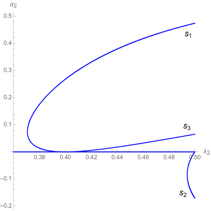
(a) The values of α1subscript𝛼1\alpha_{1} on the vertical axis plotted against the corresponding values of the third largest eigenvalue λ2subscript𝜆2\lambda_{2} on the horizontal axis.
(b)
Refer to caption
(c) The values of α2subscript𝛼2\alpha_{2} on the vertical axis plotted against the corresponding values of the third largest eigenvalue λ2subscript𝜆2\lambda_{2} on the horizontal axis.
Figure 2. The solutions to the boundary law equations (4.2), (4.3) for q=5𝑞5q=5 in terms of the Fourier modes α1,2subscript𝛼12\alpha_{1,2} depending on the third largest eigenvalue λ2subscript𝜆2\lambda_{2} of the transfer matrix M𝑀M.
Refer to caption
Refer to caption
Refer to caption
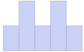
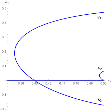
Figure 3. Symmetry of the solutions s1,s2,s3subscript𝑠1subscript𝑠2subscript𝑠3s_{1},s_{2},s_{3} in the Potts model.

All the solutions to the polynomial equation (4.6) can be calculated by numerical techniques. For a plot of the derived coefficients α1subscript𝛼1\alpha_{1} and α2subscript𝛼2\alpha_{2} respectively against the corresponding value of λ2subscript𝜆2\lambda_{2}, see Figures 2(b) and 2(c). It can be checked by simple numerical calculations that all of these solutions correspond to a probability distribution.

In accordance with our previous investigation we find that there only exists the trivial solution to the fixed-point equations if λ2<λ2csubscript𝜆2superscriptsubscript𝜆2𝑐\lambda_{2}<\lambda_{2}^{c}. At the critical value λ2csuperscriptsubscript𝜆2𝑐\lambda_{2}^{c} an additional solution away from the trivial one appears, which then undergoes a pitchfork bifurcation. For λ2=0.4subscript𝜆20.4\lambda_{2}=0.4 the lower branch then becomes 00, which happens when

e=8λ2236λ23+40λ24=0.𝑒8superscriptsubscript𝜆2236superscriptsubscript𝜆2340superscriptsubscript𝜆240e=8\lambda_{2}^{2}-36\lambda_{2}^{3}+40\lambda_{2}^{4}=0.

As we have predicted, an additional solution appears when λ2=λ~2csubscript𝜆2superscriptsubscript~𝜆2𝑐\lambda_{2}=\tilde{\lambda}_{2}^{c}. This solution then also undergoes a bifurcation for increasing values of λ2subscript𝜆2\lambda_{2} and the lower branch becomes 00 for λ2=0.5subscript𝜆20.5\lambda_{2}=0.5, which is again where e=0𝑒0e=0. So we have exactly four different solutions to our two-dimensional fixed-point equation when λ2=0.5subscript𝜆20.5\lambda_{2}=0.5 which is of course when our generalized clock model turns into the Potts model with no external magnetic field. In this situation there are three additional solutions s1,s2,s3subscript𝑠1subscript𝑠2subscript𝑠3s_{1},s_{2},s_{3} to the trivial one. The symmetries of the corresponding boundary laws are visualized in Figure 3.

In the Potts model the transition matrix can be written in the form

Mi,j={eβ/Z,if i=j1/Z,if ijsubscript𝑀𝑖𝑗casessuperscript𝑒𝛽𝑍if 𝑖𝑗1𝑍if 𝑖𝑗M_{i,j}=\begin{cases}e^{\beta}/Z,&\mbox{if }i=j\\ 1/Z,&\mbox{if }i\neq j\end{cases}

with β>0𝛽0\beta>0 and Z=eβ+q1𝑍superscript𝑒𝛽𝑞1Z=e^{\beta}+q-1 being a normalizing constant. Then λ1=λ2=eβ1eβ+q1subscript𝜆1subscript𝜆2superscript𝑒𝛽1superscript𝑒𝛽𝑞1\lambda_{1}=\lambda_{2}=\frac{e^{\beta}-1}{e^{\beta}+q-1}. Note that 2λ1=12subscript𝜆112\lambda_{1}=1 if and only if θ:=eβ=q+1assign𝜃superscript𝑒𝛽𝑞1\theta:=e^{\beta}=q+1.

Let us comment on this value. Recall that in the 555-state Potts model the translation-invariant states are described by the translation-invariant solutions for the boundary law equation [21]: There is always the free solution (corresponding to open boundary conditions), and each boundary law has the property that its 555 components take only two values. There are two different one-dimensional fixed-point equations for the case of a decomposition into either 1+4141+4 or 2+3232+3 components. Each of these fixed-point equations have different critical inverse temperatures at which solutions appear and bifurcate into an upper and a lower branch. It is a property of the recursion that on the binary tree at θ:=eβ=q+1assign𝜃superscript𝑒𝛽𝑞1\theta:=e^{\beta}=q+1 the lower branches of these recursions become equal to the free solution. This behavior is similar for all Potts models on Cayley trees of any degree and the corresponding value θcrsubscript𝜃𝑐𝑟\theta_{cr} is known [21]. As we will see shortly in Proposition 4.1 this critical value is identical with the critical value for the existence of RPT for Cayley trees of any degree.

This is remarkable. Robust phase transition is caused by local instability of the equidistribution, that is small perturbations won’t be attracted by the equidistribution but will converge to (one of) the stable symmetry breaking fixed points. On the other hand, the degeneration of the lower branches of the m𝑚m-indexed boundary laws (with m𝑚m singled out components) is indicated by the same equation. Let θRPTsubscript𝜃𝑅𝑃𝑇\theta_{RPT} denote the critical value of θ𝜃\theta for the existence of RPT in the Potts model.

Proposition 4.1.

Let T𝑇T be a Cayley tree of degree d𝑑d\in\mathbb{N}. In the Potts model with q𝑞q\in\mathbb{N} states we have

θRPT=θcr.subscript𝜃𝑅𝑃𝑇subscript𝜃𝑐𝑟\theta_{RPT}=\theta_{cr}.

Proof. It is known that θcr=d+q1d1subscript𝜃𝑐𝑟𝑑𝑞1𝑑1\theta_{cr}=\frac{d+q-1}{d-1} [21]. As θ=θRPT𝜃subscript𝜃𝑅𝑃𝑇\theta=\theta_{RPT} iff

λ1=θ1θ+q1=1dsubscript𝜆1𝜃1𝜃𝑞11𝑑\lambda_{1}=\frac{\theta-1}{\theta+q-1}=\frac{1}{d}

the claim is obviously true. \Box

4.2. Case q=4

We still consider the generalized clock model on the binary tree T𝑇T. Let the local state space be given by Ω0={0,,3}subscriptΩ003\Omega_{0}=\{0,...,3\}. Again we assume M𝑀M to be non-increasing. The entries of the first row of the transfer matrix are given by

r0=14(1+2λ1+λ2),subscript𝑟01412subscript𝜆1subscript𝜆2r_{0}=\frac{1}{4}(1+2\lambda_{1}+\lambda_{2}),
r1=14(1λ2)=r3,subscript𝑟1141subscript𝜆2subscript𝑟3r_{1}=\frac{1}{4}(1-\lambda_{2})=r_{3},
r2=14(12λ1+λ2),subscript𝑟21412subscript𝜆1subscript𝜆2r_{2}=\frac{1}{4}(1-2\lambda_{1}+\lambda_{2}),

where λi,i=0,1,2formulae-sequencesubscript𝜆𝑖𝑖012\lambda_{i},i=0,1,2 denote the eigenvalues of M𝑀M. For the basis of the mass-zero measures we choose

φ1:=c11(1,cosπ2,cosπ,cos3π2)=c11(1,0,1,0),c11:=2,formulae-sequenceassignsubscript𝜑1superscriptsubscript𝑐111𝜋2𝜋3𝜋2superscriptsubscript𝑐111010assignsuperscriptsubscript𝑐112\varphi_{1}:=c_{1}^{-1}(1,\cos\frac{\pi}{2},\cos\pi,\cos\frac{3\pi}{2})=c_{1}^{-1}(1,0,-1,0),\quad c_{1}^{-1}:=\sqrt{2},
φ2:=c21(1,cosπ,cos2π,cos3π)=c21(1,1,1,1),c21:=2.formulae-sequenceassignsubscript𝜑2superscriptsubscript𝑐211𝜋2𝜋3𝜋superscriptsubscript𝑐211111assignsuperscriptsubscript𝑐212\varphi_{2}:=c_{2}^{-1}(1,\cos\pi,\cos 2\pi,\cos 3\pi)=c_{2}^{-1}(1,-1,1,-1),\quad c_{2}^{-1}:=2.

The symmetric probability distributions can be represented as

α(j)=14+α1φ1(j)+α2φ2(j).𝛼𝑗14subscript𝛼1subscript𝜑1𝑗subscript𝛼2subscript𝜑2𝑗\alpha(j)=\frac{1}{4}+\alpha_{1}\varphi_{1}(j)+\alpha_{2}\varphi_{2}(j).

The recursion F4subscript𝐹4F_{4} of the distributions on the binary tree T𝑇T is then given by

α(j)=F4α(j):=(14+k=12λkαkφk(j))2j=03(14+k=12λkαkφk(j))2.𝛼𝑗subscript𝐹4𝛼𝑗assignsuperscript14superscriptsubscript𝑘12subscript𝜆𝑘subscript𝛼𝑘subscript𝜑𝑘𝑗2superscriptsubscript𝑗03superscript14superscriptsubscript𝑘12subscript𝜆𝑘subscript𝛼𝑘subscript𝜑𝑘𝑗2\alpha(j)=F_{4}\alpha(j):=\frac{\left(\frac{1}{4}+\sum_{k=1}^{2}\lambda_{k}\alpha_{k}\varphi_{k}(j)\right)^{2}}{\sum_{j=0}^{3}\left(\frac{1}{4}+\sum_{k=1}^{2}\lambda_{k}\alpha_{k}\varphi_{k}(j)\right)^{2}}.

The summands in the numerator are given by

(Mα(j))2=142+14(α12λ12+α22λ22)+(12λ1α1+α1α2λ1λ2)φ1(j)+(12λ2α2+12α12λ12)φ2(j).superscript𝑀𝛼𝑗21superscript4214superscriptsubscript𝛼12superscriptsubscript𝜆12superscriptsubscript𝛼22superscriptsubscript𝜆2212subscript𝜆1subscript𝛼1subscript𝛼1subscript𝛼2subscript𝜆1subscript𝜆2subscript𝜑1𝑗12subscript𝜆2subscript𝛼212superscriptsubscript𝛼12superscriptsubscript𝜆12subscript𝜑2𝑗\begin{split}(M\alpha(j))^{2}=&\frac{1}{4^{2}}+\frac{1}{4}\Big{(}\alpha_{1}^{2}\lambda_{1}^{2}+\alpha_{2}^{2}\lambda_{2}^{2}\Big{)}+\Big{(}\frac{1}{2}\lambda_{1}\alpha_{1}+\alpha_{1}\alpha_{2}\lambda_{1}\lambda_{2}\Big{)}\varphi_{1}(j)\\ &+\Big{(}\frac{1}{2}\lambda_{2}\alpha_{2}+\frac{1}{2}\alpha_{1}^{2}\lambda_{1}^{2}\Big{)}\varphi_{2}(j).\end{split}

By orthogonality the normalization is just

j=03(Mα(j))2=14+α12λ12+α22λ22superscriptsubscript𝑗03superscript𝑀𝛼𝑗214superscriptsubscript𝛼12superscriptsubscript𝜆12superscriptsubscript𝛼22superscriptsubscript𝜆22\sum_{j=0}^{3}(M\alpha(j))^{2}=\frac{1}{4}+\alpha_{1}^{2}\lambda_{1}^{2}+\alpha_{2}^{2}\lambda_{2}^{2}

and hence

F4α(j)=14+12λ1α1+α1α2λ1λ214+α12λ12+α22λ22φ1(j)+12λ2α2+12α12λ1214+α12λ12+α22λ22φ2(j).subscript𝐹4𝛼𝑗1412subscript𝜆1subscript𝛼1subscript𝛼1subscript𝛼2subscript𝜆1subscript𝜆214superscriptsubscript𝛼12superscriptsubscript𝜆12superscriptsubscript𝛼22superscriptsubscript𝜆22subscript𝜑1𝑗12subscript𝜆2subscript𝛼212superscriptsubscript𝛼12superscriptsubscript𝜆1214superscriptsubscript𝛼12superscriptsubscript𝜆12superscriptsubscript𝛼22superscriptsubscript𝜆22subscript𝜑2𝑗F_{4}\alpha(j)=\frac{1}{4}+\frac{\frac{1}{2}\lambda_{1}\alpha_{1}+\alpha_{1}\alpha_{2}\lambda_{1}\lambda_{2}}{\frac{1}{4}+\alpha_{1}^{2}\lambda_{1}^{2}+\alpha_{2}^{2}\lambda_{2}^{2}}\varphi_{1}(j)+\frac{\frac{1}{2}\lambda_{2}\alpha_{2}+\frac{1}{2}\alpha_{1}^{2}\lambda_{1}^{2}}{\frac{1}{4}+\alpha_{1}^{2}\lambda_{1}^{2}+\alpha_{2}^{2}\lambda_{2}^{2}}\varphi_{2}(j).

This leads to the two fixed-point equations

(4.7) α1=12λ1α1+α1α2λ1λ214+α12λ12+α22λ22,α2=12λ2α2+12α12λ1214+α12λ12+α22λ22.formulae-sequencesubscript𝛼112subscript𝜆1subscript𝛼1subscript𝛼1subscript𝛼2subscript𝜆1subscript𝜆214superscriptsubscript𝛼12superscriptsubscript𝜆12superscriptsubscript𝛼22superscriptsubscript𝜆22subscript𝛼212subscript𝜆2subscript𝛼212superscriptsubscript𝛼12superscriptsubscript𝜆1214superscriptsubscript𝛼12superscriptsubscript𝜆12superscriptsubscript𝛼22superscriptsubscript𝜆22\begin{split}\alpha_{1}&=\frac{\frac{1}{2}\lambda_{1}\alpha_{1}+\alpha_{1}\alpha_{2}\lambda_{1}\lambda_{2}}{\frac{1}{4}+\alpha_{1}^{2}\lambda_{1}^{2}+\alpha_{2}^{2}\lambda_{2}^{2}},\\ \alpha_{2}&=\frac{\frac{1}{2}\lambda_{2}\alpha_{2}+\frac{1}{2}\alpha_{1}^{2}\lambda_{1}^{2}}{\frac{1}{4}+\alpha_{1}^{2}\lambda_{1}^{2}+\alpha_{2}^{2}\lambda_{2}^{2}}.\end{split}

For the critical value λ1=1/2subscript𝜆112\lambda_{1}=1/2 it follows from the first of these equations that α1=0subscript𝛼10\alpha_{1}=0 or

(4.8) α1=±2λ2α24λ22α22.subscript𝛼1plus-or-minus2subscript𝜆2subscript𝛼24superscriptsubscript𝜆22superscriptsubscript𝛼22\begin{split}\alpha_{1}=\pm\sqrt{2\lambda_{2}\alpha_{2}-4\lambda_{2}^{2}\alpha_{2}^{2}}.\end{split}

In the case where α1=±2λ2α24λ22α22subscript𝛼1plus-or-minus2subscript𝜆2subscript𝛼24superscriptsubscript𝜆22superscriptsubscript𝛼22\alpha_{1}=\pm\sqrt{2\lambda_{2}\alpha_{2}-4\lambda_{2}^{2}\alpha_{2}^{2}}, it follows from the second fixed-point equation that

α2=3λ212(λ2+λ22).subscript𝛼23subscript𝜆212subscript𝜆2superscriptsubscript𝜆22\alpha_{2}=\frac{3\lambda_{2}-1}{2(\lambda_{2}+\lambda_{2}^{2})}.

Plugging this value for α2subscript𝛼2\alpha_{2} into (4.8), we get that ±2λ2α24λ22α22plus-or-minus2subscript𝜆2subscript𝛼24superscriptsubscript𝜆22superscriptsubscript𝛼22\pm\sqrt{2\lambda_{2}\alpha_{2}-4\lambda_{2}^{2}\alpha_{2}^{2}} only takes real values if and only if λ2(1/3,1)subscript𝜆2131\lambda_{2}\in(1/3,1). Hence the critical value for λ2subscript𝜆2\lambda_{2} for the existence of a phase transition is λ2c:=13assignsuperscriptsubscript𝜆2𝑐13\lambda_{2}^{c}:=\frac{1}{3}. An easy calculation shows that all the solutions to (4.7) correspond to a probability distribution. We have thereby shown the following theorem.

Theorem 4.2.

Consider the 444-state generalized clock model on the binary tree where the critical value for RPT is λ1=1/2subscript𝜆112\lambda_{1}=1/2. Then the spin model has Gibbs measures with single-site marginals different from the equidistribution if and only if λ2(1/3,1/2)subscript𝜆21312\lambda_{2}\in(1/3,1/2).

We have seen that there exist non-robust phase transitions in the generalized clock model on the binary tree for q{4,5}𝑞45q\in\{4,5\}. It is not difficult to prove that for a generalized clock model on a tree T𝑇T which exhibits no RPT there always exists another tree Tsuperscript𝑇T^{\prime} s.t. brT=brTbr𝑇brsuperscript𝑇\operatorname{br}T=\operatorname{br}T^{\prime} and Tsuperscript𝑇T^{\prime} does not exhibit a PT. This is very much done by the same techniques proving the absence of RPT under the condition λ1brT<1subscript𝜆1br𝑇1\lambda_{1}\operatorname{br}T<1. The tree Tsuperscript𝑇T^{\prime} is constructed by adding edges in series with sufficient length to the tree T𝑇T, where the adding of these edges must be done sufficiently sparse such that brT=brTbr𝑇brsuperscript𝑇\operatorname{br}T=\operatorname{br}T^{\prime}. The recursion along these added series of edges then replaces the weakening of the coupling along the cutset in the notion of RPT (see the proof of Theorem 1.14 in [29]).
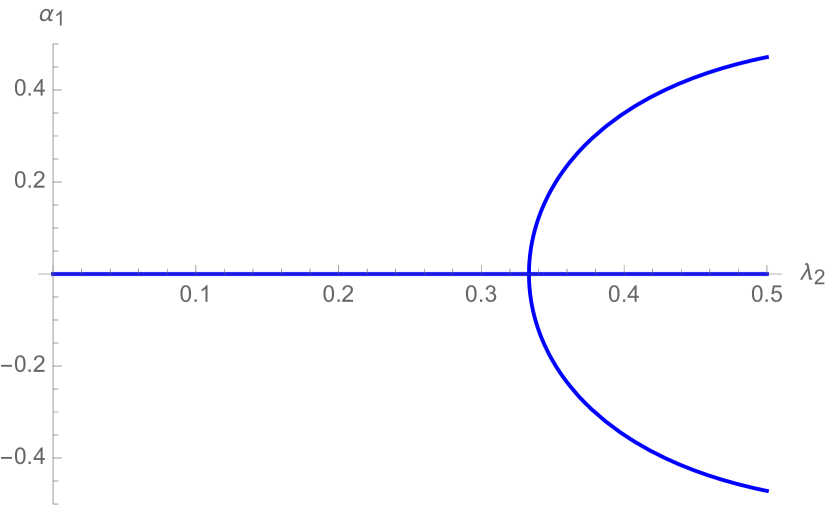
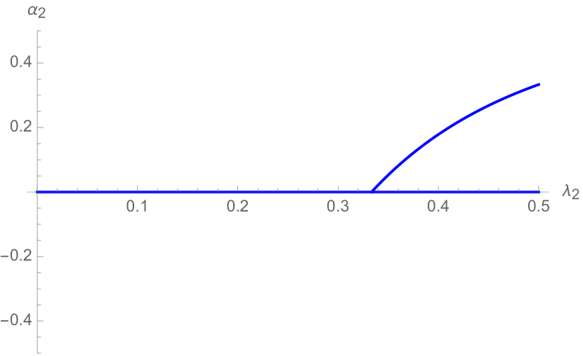
Refer to caption
Refer to caption
Figure 4. The solutions to the boundary law equations (4.2), (4.3) for q=4𝑞4q=4 in terms of the Fourier modes α1,2subscript𝛼12\alpha_{1,2} depending on the third largest eigenvalue λ2subscript𝜆2\lambda_{2}.

Let us map our solutions to the known solutions of the Potts model [21]. Note that at λ1=1/2subscript𝜆112\lambda_{1}=1/2 there is a bifurcation of the m=2𝑚2m=2 branches from the free solution α=1𝛼1\alpha=1, where both branches exist only for bigger values of λ1subscript𝜆1\lambda_{1}. Hence the only available solution is of type m=1𝑚1m=1, and here we only find the solution of the upper branch of the form, written in boundary law language, (a,1,1,1),a1𝑎111𝑎1(a,1,1,1),a\neq 1. Also, our recursion acts in the subspace of these solutions which are symmetric w.r.t. 00. Hence only two of the possible permutations persist, namely (a,1,1,1),(1,1,a,1)𝑎11111𝑎1(a,1,1,1),(1,1,a,1). These solutions are mapped to the upper and lower end of the pitchfork type branches in Figure 4.

In the Potts model the transfer matrix is given by M(i,j)=exp[β𝟏{i=j}]𝑀𝑖𝑗𝛽subscript1𝑖𝑗M(i,j)=\exp[\beta\mathbf{1}_{\{i=j\}}] with inverse temperature β>0𝛽0\beta>0. It is known that the effective inverse temperature for the existence of a PT in the Potts model is given by βc=12log(1+2q1)subscript𝛽𝑐1212𝑞1\beta_{c}=\frac{1}{2}\log(1+2\sqrt{q-1}). As the second largest eigenvalue is given by λ2=eβeβeβ+(q1)eβsubscript𝜆2superscript𝑒𝛽superscript𝑒𝛽superscript𝑒𝛽𝑞1superscript𝑒𝛽\lambda_{2}=\frac{e^{\beta}-e^{-\beta}}{e^{\beta}+(q-1)e^{-\beta}} we get for the critical value λ2c=2q1q+2q1superscriptsubscript𝜆2𝑐2𝑞1𝑞2𝑞1\lambda_{2}^{c}=\frac{2\sqrt{q-1}}{q+2\sqrt{q-1}}. For q=4,5𝑞45q=4,5 we have given the exact transition point for the existence of (non-robust) phase transitions at criticality, i.e. for λ1=1/2subscript𝜆112\lambda_{1}=1/2. For the case q=4𝑞4q=4 we can even calculate the critical value λ2csuperscriptsubscript𝜆2𝑐\lambda_{2}^{c} for the existence of non-robust phase transitions for any value of λ1[0,1/2]subscript𝜆1012\lambda_{1}\in[0,1/2]: For α10subscript𝛼10\alpha_{1}\neq 0 we get from the first equation of (4.7) that

(4.9) α12λ12=12λ1+λ1λ2α214λ22α22=:P1(α2).\begin{split}\alpha_{1}^{2}\lambda_{1}^{2}&=\frac{1}{2}\lambda_{1}+\lambda_{1}\lambda_{2}\alpha_{2}-\frac{1}{4}-\lambda_{2}^{2}\alpha_{2}^{2}=:P_{1}(\alpha_{2}).\end{split}

The second equation of (4.7) gives us

(4.10) α12λ12=λ2α2+λ1α2+2λ1λ2α22=:P2(α2).\begin{split}\alpha_{1}^{2}\lambda_{1}^{2}&=-\lambda_{2}\alpha_{2}+\lambda_{1}\alpha_{2}+2\lambda_{1}\lambda_{2}\alpha_{2}^{2}=:P_{2}(\alpha_{2}).\end{split}

The critical line in (λ1,λ2)subscript𝜆1subscript𝜆2(\lambda_{1},\lambda_{2})-space for the existence of multiple solutions to (4.7) are given by the two equations P1(α2)=P2(α2)subscript𝑃1subscript𝛼2subscript𝑃2subscript𝛼2P_{1}(\alpha_{2})=P_{2}(\alpha_{2}) and P1(α2)=P2(α2)superscriptsubscript𝑃1subscript𝛼2superscriptsubscript𝑃2subscript𝛼2P_{1}^{\prime}(\alpha_{2})=P_{2}^{\prime}(\alpha_{2}). They are derived by the requirement that the parabolas described by P1subscript𝑃1P_{1} and P2subscript𝑃2P_{2} as a function of α2subscript𝛼2\alpha_{2} have precisely one touching point described by a critical α2subscript𝛼2\alpha_{2}. It can be shown by elementary computations eliminating the α2subscript𝛼2\alpha_{2} that the solutions to this system are given by λ1=4λ21λ2(1+λ2)2subscript𝜆14subscript𝜆21subscript𝜆2superscript1subscript𝜆22\lambda_{1}=4\lambda_{2}\frac{1-\lambda_{2}}{(1+\lambda_{2})^{2}}. The critical points are given by the dashed line in Figure 5.
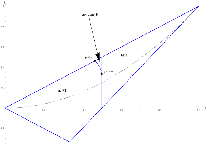
Refer to caption
Figure 5. The generalized clock model for q=4𝑞4q=4 can be described by the two eigenvalues λ1,2subscript𝜆12\lambda_{1,2} of the transfer matrix M𝑀M. The region for the existence of non-robust phase transitions is given by the area above the dashed line inside the quadrangle. Note that the transition point in the Potts model is given by λ1=λ2=2q1q+2q10.4641subscript𝜆1subscript𝜆22𝑞1𝑞2𝑞10.4641\lambda_{1}=\lambda_{2}=\frac{2\sqrt{q-1}}{q+2\sqrt{q-1}}\approx 0.4641 and the transition point at the critical value for RPT in the generalized clock model on the binary tree is given by λ1=1/2subscript𝜆112\lambda_{1}=1/2 and λ2=1/3subscript𝜆213\lambda_{2}=1/3. The eigenvalues of the transition matrix for the standard-clock model with scalarproduct-interaction are given by the dotted line. There are no non-robust PTs in the standard clock model.
Refer to caption
Figure 6. The generalized clock model for q=5𝑞5q=5 can be described by the two eigenvalues λ1,2subscript𝜆12\lambda_{1,2} of the transfer matrix M𝑀M. The region for the existence of non-robust phase transitions is given by the area above the dashed line inside the triangle. The eigenvalues for the standard-clock model are given by the dotted line.
Refer to caption
Figure 7. In the Potts regime the values of the determinant of the Jacobi matrix of (4.12) for α1=α2=α±subscript𝛼1subscript𝛼2subscript𝛼plus-or-minus\alpha_{1}=\alpha_{2}=\alpha_{\pm} are plotted against λ=λ1=λ2𝜆subscript𝜆1subscript𝜆2\lambda=\lambda_{1}=\lambda_{2}.

For q=5𝑞5q=5 the task to determine the transition line between the two regimes becomes more difficult. However, it is possible to use the implicit function theorem to prove the existence of non-robust phase transitions. In the Potts regime with λ1=λ2=λsubscript𝜆1subscript𝜆2𝜆\lambda_{1}=\lambda_{2}=\lambda and λ(4/9,1/2)𝜆4912\lambda\in(4/9,1/2) there exist two b.l. solutions of the form l=(a±,1,1,1,1)𝑙subscript𝑎plus-or-minus1111l=(a_{\pm},1,1,1,1) with

(4.11) a±=(1eβ2(q1)±54q2eβ+e2β2(q1))1subscript𝑎plus-or-minussuperscriptplus-or-minus1superscript𝑒𝛽2𝑞154𝑞2superscript𝑒𝛽superscript𝑒2𝛽2𝑞11\begin{split}a_{\pm}=\left(\frac{1-e^{\beta}}{2(q-1)}\pm\frac{\sqrt{5-4q-2e^{\beta}+e^{2\beta}}}{2(q-1)}\right)^{-1}\end{split}

where eβ=1+λ(q1)1λsuperscript𝑒𝛽1𝜆𝑞11𝜆e^{\beta}=\frac{1+\lambda(q-1)}{1-\lambda}. Here, λ𝜆\lambda is the only non-trivial eigenvalue of the transfer matrix M𝑀M. The Fourier modes α1±,α2±superscriptsubscript𝛼1plus-or-minussuperscriptsubscript𝛼2plus-or-minus\alpha_{1}^{\pm},\alpha_{2}^{\pm} of the solutions a±subscript𝑎plus-or-minusa_{\pm} are then given by α1±=α2±=2(1a±)5superscriptsubscript𝛼1plus-or-minussuperscriptsubscript𝛼2plus-or-minus21subscript𝑎plus-or-minus5\alpha_{1}^{\pm}=\alpha_{2}^{\pm}=\frac{2(1-a_{\pm})}{5}. Let T:22:𝑇superscript2superscript2T:\mathbb{R}^{2}\to\mathbb{R}^{2} be defined by

(4.12) T(α1,α2)=(α1115+α12λ12+α22λ22(25λ1α1+2λ1λ2vα1α2+vλ22α22)α2115+α12λ12+α22λ22(25λ2α2+2λ1λ2vα1α2+vλ12α12)).𝑇subscript𝛼1subscript𝛼2matrixsubscript𝛼1115superscriptsubscript𝛼12superscriptsubscript𝜆12superscriptsubscript𝛼22superscriptsubscript𝜆2225subscript𝜆1subscript𝛼12subscript𝜆1subscript𝜆2𝑣subscript𝛼1subscript𝛼2𝑣superscriptsubscript𝜆22superscriptsubscript𝛼22subscript𝛼2115superscriptsubscript𝛼12superscriptsubscript𝜆12superscriptsubscript𝛼22superscriptsubscript𝜆2225subscript𝜆2subscript𝛼22subscript𝜆1subscript𝜆2𝑣subscript𝛼1subscript𝛼2𝑣superscriptsubscript𝜆12superscriptsubscript𝛼12T(\alpha_{1},\alpha_{2})=\begin{pmatrix}\alpha_{1}-\frac{1}{\frac{1}{5}+\alpha_{1}^{2}\lambda_{1}^{2}+\alpha_{2}^{2}\lambda_{2}^{2}}\left(\frac{2}{5}\lambda_{1}\alpha_{1}+2\lambda_{1}\lambda_{2}v\alpha_{1}\alpha_{2}+v\lambda_{2}^{2}\alpha_{2}^{2}\right)\\ \alpha_{2}-\frac{1}{\frac{1}{5}+\alpha_{1}^{2}\lambda_{1}^{2}+\alpha_{2}^{2}\lambda_{2}^{2}}\left(\frac{2}{5}\lambda_{2}\alpha_{2}+2\lambda_{1}\lambda_{2}v\alpha_{1}\alpha_{2}+v\lambda_{1}^{2}\alpha_{1}^{2}\right)\end{pmatrix}.

To apply the implicit function theorem we need to compute and discuss the Jacobian. We don’t give details, but provide a plot of the Jacobian of T𝑇T for λ1=λ2subscript𝜆1subscript𝜆2\lambda_{1}=\lambda_{2} and α1=α2=α±subscript𝛼1subscript𝛼2subscript𝛼plus-or-minus\alpha_{1}=\alpha_{2}=\alpha_{\pm} which is given in Figure 7. Note that the Jacobi matrix becomes non-invertible right at the critical value for the existence of RPT, i.e., λ1=λ2=1/2subscript𝜆1subscript𝜆212\lambda_{1}=\lambda_{2}=1/2. This is the point where the lower branch of the b.l. solutions, i.e. asubscript𝑎a_{-}, turns into the free solution. For λ1=λ2(4/9,1/2)subscript𝜆1subscript𝜆24912\lambda_{1}=\lambda_{2}\in(4/9,1/2) the Jacobian is always invertible at the Potts solution. Hence for every λ1=λ2subscript𝜆1subscript𝜆2\lambda_{1}=\lambda_{2} there exists an open neighborhood around that point in which there exist non-robust phase transitions. Even though we did not give an analytic argument to show the form of the transition line between the regimes PT=RPT and PT\neqRPT, we can compute it numerically. The transition line for the case q=5𝑞5q=5 is given by the dashed line in Figure 6.

Acknowledgement

This work is supported by Deutsche Forschungsgemeinschaft, RTG 2131 High-dimensional Phenomena in Probability - Fluctuations and Discontinuity. We thank Aernout van Enter for useful comments to an earlier draft of the manuscript.

References

  • [1] R. Bissacot, E. O. Endo, A. C. D. van Enter, Stability of the phase transition of critical-field Ising model on Cayley trees under inhomogeneous external fields, arXiv: 1611.00424, 2016.
  • [2] P. M. Blekher, N. N. Ganikhodzhaev, Pure phases of the Ising model on Bethe lattices, Theory Probab. Appl., 35, No. 2, 216-227, 1990.
  • [3] C. Borgs, R. Kotecký, I. Medved’, Finite-size effects for the Potts model with weak boundary conditions, J. Stat. Phys., 109, No. 1, 67-131, 2002.
  • [4] A. Dembo, A. Montanari, Ising models on locally tree-like graphs, Ann. Appl. Probab., 20, No. 2, 565-592, 2010.
  • [5] A. Dembo, A. Montanari, N. Sun, Factor models on locally tree-like graphs, Ann. Probab., 41, No. 6, 4162-4213, 2013.
  • [6] S. Dommers, C. Giardinà, R. van der Hofstad, Ising critical exponents on random trees and graphs, Comm. Math. Phys., 328, No. 1, 355-395, 2014.
  • [7] S. Dommers, C. Külske, P. Schriever, Continuous spin models on annealed generalized random graphs, arXiv: 1610.08242, 2016.
  • [8] A. C. D. van Enter, R. Fernández, A. D. Sokal, Regularity properties and pathologies of position-space renormalization-group transformations: Scope and limitations of Gibbsian theory, J. Stat. Phys., 72, No. 5, 879-1167, 1993.
  • [9] A. C. D. van Enter, A remark on the notion of robust phase transitions, J. Stat. Phys., 98, No. 5/6, 1409-1416, 2000.
  • [10] A. C. D. van Enter, I. Medved’, K. Netočný, Chaotic size dependence in the Ising model with random boundary conditions, Markov Process. Related Fields, 8, No. 3, 479-508, 2002.
  • [11] A. C. D. van Enter, V. Ermolaev, G. Iacobelli, C. Külske, Gibbs-non-Gibbs properties for evolving Ising models on trees, Ann. Inst. Henri Poincaré Probab. Stat., 48, No. 3, 774-791, 2012.
  • [12] A. C. D. van Enter, C. Külske, A. Opoku, Discrete approximations to vector spin models, J. Phys. A: Math. Theor., 44, 2011.
  • [13] J. Fröhlich, T. Spencer, The Kosterlitz-Thouless transition in two-dimensional Abelian spin systems and the Coulomb gas, Comm. Math. Phys., 81, No. 4, 527-602, 1981.
  • [14] M. Formentin, C. Külske, On the purity of the free boundary condition Potts measure on random trees, Stoch. Process. Appl., 119, No. 9, 2992-3005, 2009.
  • [15] H. Furstenberg, Intersections of Cantor sets and transversality of semigroups. In: R. C. Gunning, editor, Problems in Analysis, A symposium in honor of Salomon Bochner, pages 41-59. Princeton Univ. Press, Princeton, N.J., 1970
  • [16] D. Gandolfo, J. Ruiz, S. Shlosman, A manifold of pure Gibbs states of the Ising model on a Cayley tree, J. Stat. Phys., 148, No. 6, 999-1005, 2012.
  • [17] N. N. Ganikhodzhaev, U. A. Rozikov, Description of periodic extreme Gibbs measures of some lattice models on a Cayley tree, Theoret. and Math. Phys., 111, No. 1, 480-486, 1997.
  • [18] H. O. Georgii, Gibbs Measures and Phase Transitions, 2nd ed., de Gruyter Studies in Mathematics 9, Walter de Gruyter & Co., Berlin, 2011.
  • [19] B. Jahnel, C. Külske, A class of nonergodic interacting particle systems with unique invariant measure, Ann. Appl. Probab, 24, No. 6, 2595-2643, 2014.
  • [20] S. Janson, E. Mossel, Robust reconstruction on trees is determined by the second eigenvalue, Ann. Probab., 32, No.3B, 2630-2649, 2004.
  • [21] C. Külske, U. Rozikov, R.M. Khakimov, Description of the translation-invariant splitting Gibbs measures for the Potts model on a Cayley tree, J. Stat. Phys., 156, No. 1, 189-200, 2014.
  • [22] C. Külske, U. Rozikov, Fuzzy transformations and extremality of Gibbs measures for the Potts model on a Cayley tree, Random Struct. Alg., doi:10.1002/rsa.20671
  • [23] C. Külske, P. Schriever, Gradient Gibbs measures and fuzzy transformations on trees, Preprint, arXiv: 1609.00159, 2016.
  • [24] R. Lyons, Y. Peres, Probability on Trees and Networks, Cambridge Series in Statistical and Probabilistic Mathematics, Cambridge University Press, Cambridge, 2016.
  • [25] R. Lyons, The Ising model and percolation on trees and tree-like graphs, Comm. Math. Phys., 125, No. 2, 337-353, 1989
  • [26] R. Lyons, Random walks and percolation on trees, Ann. Probab., 18, No.3, 931-958, 1990
  • [27] C. Maes, S. Shlosman, Rotating states in driven clock- and XY-models, J. Stat. Phys., 144, No. 6, 1238-1246, 2011.
  • [28] R. Pemantle, Y. Peres, The Critical Ising Model on Trees, Concave Recursions and Nonlinear Capacity, Ann. Probab., 38, No.1, 184-206, 2010.
  • [29] R. Pemantle, J. Steif, Robust phase transitions for Heisenberg and other models on general trees, Ann. Probab., 27, No. 2, 876-912, 1999.
  • [30] E. L. Rees, Discussion of the roots of a quartic function, Amer. Math. Monthly, 29, No. 2, 51-55, 1922.
  • [31] U. Rozikov, Gibbs Measures on Cayley Trees, Word Scientific, Singapore, 2013.
  • [32] A. Sly, Reconstruction for the Potts model, Ann. Probab., 39, No. 4, 1365-1406, 2011.
  • [33] S. Zachary, Countable state space Markov random fields and Markov chains on trees, Ann. Probab., 11, No. 4, 894-903, 1983.