Initial Estimates on the Performance of the LSST on the Detection of Eclipsing Binaries

Abstract

In this work we quantify the performance of LSST on the detection of eclipsing binaries. We use Kepler observed binaries to create a large sample of simulated pseudo-LSST binary light curves. From these light curves, we attempt to recover the known binary signal. The success rate of period recovery from the pseudo-LSST light curves is indicative of LSST’s expected performance. Using an off-the-shelf Analysis of Variance (AoV) routine, we successfully recover 71% of the targets in our sample. We examine how the binary period impacts recovery success and see that for periods longer than 10 days the chance of successful binary recovery drops below 50%.

1 Introduction

1.1 LSST and Kepler

The Large Synoptic Survey Telescope (LSST) is unlike any previous telescope survey. Capable of imaging the entire sky approximately four times in a single week, the amount of data it will generate is substantial: the 3.2-gigapixel camera will take approximately 1000 pairs of exposures generating roughly 15 Terabytes of data each night. Currently under construction in Chile, the ten-year survey is expected to begin in 2022. The LSST fast cadence makes LSST appealing for the study eclipsing binaries, especially at the faint end where such an extensive survey was hereunto not possible.

The value of eclipsing binaries cannot be overstated. Aside from being exquisite distance estimators [Ribas et al., 2005], binary stars allow for direct, model-independent, measures of stellar mass [Torres et al., 2010]. The eclipses provide the relative stellar radii, the inclination of the system, and orbital characteristics such as the eccentricity and the argument of periastron. Even without radial velocities, relative radius estimates can be made for systems.

LSST will allow us to perform large scale binary population studies. One aspect that LSST will be uniquely equipped to study is binary rates as a function of spectral type, especially at the low mass end. At the high mass end, at least 75% of O-type stars form in binary or multiple systems [Mason et al., 1998, 2009]. Lower mass stars are less likely to be found in binaries: 70% of B-types and A-types [Shatsky and Tokovinin, 2002, Kobulnicky and Fryer, 2007, Kouwenhoven et al., 2007], roughly 50% of solar-types [Raghavan et al., 2010], and M-Dwarfs estimates range between 11% [Reid and Gizis, 1997] up to 34-42% [Henry and McCarthy, 1990, Fischer and Marcy, 1992]. For the least massive stars and brown dwarfs, it is estimated that only 10%-30% of stars exist in multi-star systems [Burgasser et al., 2003, Siegler et al., 2005, Allen et al., 2007, Maxted et al., 2008, Joergens, 2008].

More massive stars form in massive gas clouds which tend to form multiple stars closer together, leading to the formation of systems with multiple companions. As can be seen from the previously stated multiplicity rates, the less massive a star, the smaller the multiplicity rate. This, compounded with their faintness, makes low mass binaries difficult to study. LSST will be able to survey faint M-M binary pairs thanks to its large étendue.

In order to estimate LSST’s performance on observing eclipsing binary systems we look to NASA’s Kepler mission [Borucki et al., 2010]. This mission was designed to discover Earth-size exoplanets in or near the habitable zones of their host stars using the transit method of planet detection. This method requires a convenient orientation of the system being observed: the plane of the planet’s orbit must be aligned with the line of sight such that the planet will pass in front of the parent star and block some of its light. The Kepler telescope was launched on March 7, 2009 into an Earth-trailing orbit about the Sun to achieve a high pointing stability. Kepler produced observations of unprecedented quality in terms of sensitivity and duration. It created a superb sample of binaries due to long cadence of approximately 30 minutes, short cadence of approximately 1 minute, mission lifetime of 4 years, and observations of approximately 200,000 targets. The Kepler Eclipsing Binary Catalog (KEBC) [Prša et al., 2011, Slawson et al., 2011, Kirk et al., 2016, Abdul-Masih et al., 2016] provides a robust and vetted list of 2876 binaries as of July 1, 2016. The list of the catalog fields and a short description of each is given in Table 1.

Table 1: Column names given in the KEBC with a short description.

Catalog Column Name	Description
KIC	the Kepler input catalog identification number
period	the period of the binary
period error	the associated uncertainty in the period
bjd0	time of primary eclipse
bjd0 error	uncertainty in bjd0
GLon	galactic longitude
GLat	galactic latitude
kmag	Kepler magnitude
LC data	long cadence Kepler archived data
SC data	short cadence Kepler archived data

1.2 Simulation Overview

The KEBC sources served as templates which we used to generate light curves that resemble what LSST will observe. First, we considered a region of the sky for which we have a fairly complete sampling, namely the Kepler field. We then use this field to create a sample field in the Southern hemisphere along the same galactic latitude, in order to preserve the stellar number density. LSST’s performance on this equivalent field is evaluated by simulating observations of these sources according to the LSST cadence.

The LSST cadence will be non-uniform and determined by a multitude of inputs. Weather conditions, slew distance, and science goals are all considered when determining which part of the sky to observe next. The next field LSST observes is determined by optimization of all of these conditions. Until LSST is actually in operation, we can only simulate its observing cadence. The LSST science team has developed the LSST Operations Simulator (OpSim, Delgado et al. 2014) which will enable the simulation of the LSST cadence. The cadence of the light curves was extracted from OpSim using the Metrics Analysis Framework (MAF, Jones et al. 2014). OpSim and MAF are developed as part of the overall LSST simulations effort [Connolly et al., 2014]. Finally, the pseudo-LSST light curves were interpolated from the KEBC light curves using the LSST cadence. We neglect targets with multiple binary signals (i.e. systems with more than two members) in this current treatment.

We next attempt to recover the binary signal from the newly created light curves. For a target to be considered recovered as a binary, the strongest period will need to be a harmonic (integer multiple or fraction) of the known KEBC period.

This work serves as a proof of concept and a first step that will lead to a more sophisticated analysis including the production of an eclipsing binary science metric for use in the construction of LSST’s observing cadence.

2 Simulated Pseudo-LSST Light Curves

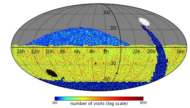
A modification was made to the KEBC light curves to make them appropriate for this work. Because Kepler observed a fixed region in the Northern hemisphere (RA 19h22m40s, Dec +44°30'00"), it was necessary to translate the dataset to the southern sky and into the viewing range of LSST. To achieve this, the galactic longitude ($l$) was inverted for each KEBC target such that $l\rightarrow-l$. By applying this transformation we are able to preserve the galactic latitude of our sample, which builds on the assumption that the number density of stars is, in general, uniform along galactic latitude. The result of this operation is depicted in Figure 1.

Figure 1: Plots of the simulated number of visits LSST will make over its planned 10 year mission lifetime. A log scale was chosen to emphasize the different observing strategies LSST will employ. Left: Plotted in equatorial coordinates with the Kepler field in white and the translated field in black. Right: Plotted in galactic coordinates with the Kepler field in white and the translated field in black.

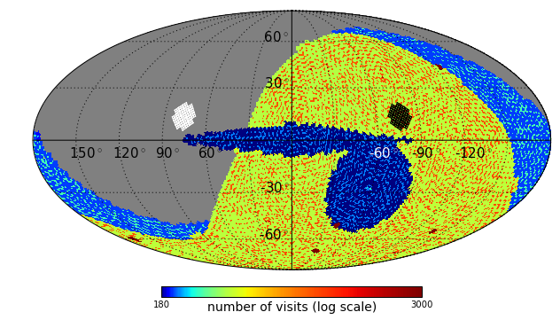Comparing the Kepler field coverage, 115 deg², to the LSST field of view per exposure, 9.6 deg², shows that roughly 11 LSST fields would cover the Kepler field. This also demonstrates that the Kepler field is a large enough patch of sky to provide multiple pointings and hence will allow separate cadences to be generated for samples.

3 LSST Simulations

The actual LSST observing cadence will be determined as the mission progresses, with changes occurring on a nightly basis due to factors such as changing weather conditions. Therefore, the ten-year observing strategy must be simulated.

OpSim is a tool that generates a realistic pointing history for LSST [Delgado et al., 2014]. OpSim takes many factors into account: realistic weather conditions such as clouds, and their effect on seeing; downtime due to scheduled as well as unscheduled maintenance; a high-fidelity model of the telescope behavior including slew time and filter changes; and a scheduler that selects desired observations for each pointing. OpSim outputs information about each observation that was simulated (e.g., epoch, sky position, seeing, sky brightness).

The current reference baseline run (minion_1016) was processed with OpSim and the output was then analyzed using MAF. For this treatment we use MAF to retrieve the exposure times for our binary targets. MAF allows for metrics to be defined that measure quantities of interest from OpSim’s simulation of the pointing history.

3.1 Light Curve Creation

A UserPointSlicer was used to obtain the exposure times. This slicer accepts a list of RA and Dec coordinates as input and returns a nested list of the exposure times for each point defined by the user.

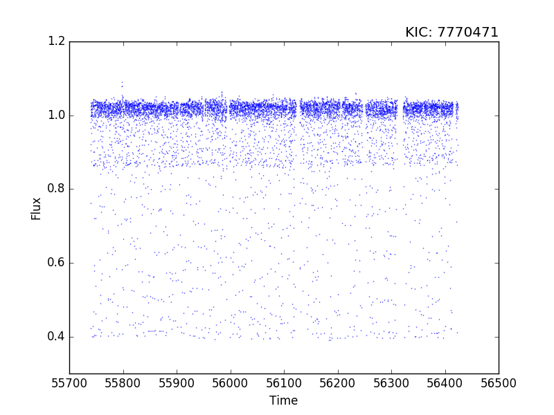
The time stamps for each KEBC binary were phase-folded over their respective period. The flux values were not simulated, instead we adopted the interpolated flux values from the Kepler phase-folded light curve. This flux interpolation is effectively sampling the Kepler light curve with the LSST cadence. The resulting pseudo-LSST phase-folded light curve is then unfolded back into time domain, producing an LSST light curve. Flux uncertainties were similarly interpolated and adopted.

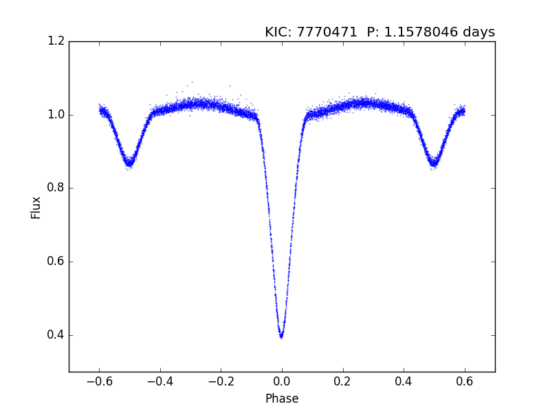
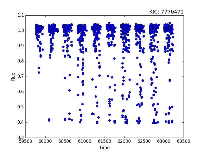
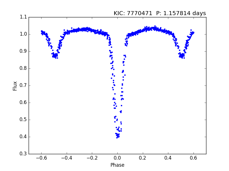
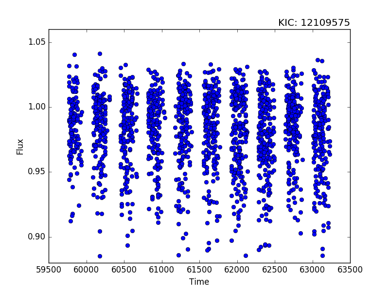
These light curves are LSST-like, meaning that the time domains are representative of what one would expect. However, it is worth pointing out the differences between these missions. The Kepler instrument used single broad band photometry while LSST will have 6 passbands, ugrizy, preferentially making observations in the r- and i-bands. The magnitude limit of each mission is also vastly different. LSST’s main survey will observe down to a typical r magnitude of 24.5 [Ivezić et al., 2008], while Kepler had a breakdown limit of approximately 19^th magnitude [Van Cleve and Caldwell, 2009]. We use flux values which are derived from Kepler and no conversion factors or corrections were made beyond the detrending which was applied to the original light curves. The flux uncertainties are certainly problematic as they are reflective of Kepler’s systematics and data acquisition. Therefore, these light curves can at this time provide only qualitative insight, quantifying only how the cadence of LSST will impact the detection of binary stars. Figure 2 shows a KEBC light curve in the top panels and the simulated LSST light curve in the bottom panels.

Figure 2: Top Left: Original Kepler light curve. Top Right: The light curve phase-folded over the KEBC period. Bottom Left: LSST simulated light curve. Bottom Right: The light curve phase-folded over the AoV period.

For reference we present a plot of a typical window function for LSST in Figure 3.

Figure 3: The window function of a constant source as observed by LSST. The diurnal cycle can be clearly seen.

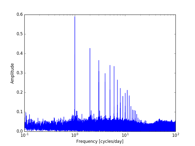
The diurnal cycle is obvious and will be present in all of the data. Red noise (cf. Pont et al. [2006]) is expected to be relatively low for LSST. This expectation is based upon the irregularity of the LSST cadence as red-noise is most notable in back-to-back time-series. However, it should be noted that the OpSim simulator does not provide enough fidelity at this time to determine the impact and influence of red noise.

LSST has a limiting magnitude of 15.8 for a 15-second $r$ band exposure [LSST Science Collaboration et al., 2009]. Therefore, we look at what precision LSST could achieve while looking at a $16^{\textnormal{th}}$ mag point source in $r$. Ivezić et al. [2008] gives the random photometric error for a single LSST visit, $\sigma_{\textnormal{rand}}$, of a point source of a certain magnitude, $m$, as

$$\sigma^{2}_{\textnormal{rand}}=(0.04-\gamma)x+\gamma x^{2}\hskip 5.0pt(\textnormal{mag}^{2})$$

with $x\equiv 10^{0.4(m-m_{5})}$. The $\gamma$ term collects a number of factors including sky brightness and readout noise among others, while $m_{5}$ is the $5\sigma$ depth for a specific band. Ivezić et al. [2008] gives a value of 0.039 for $\gamma$. The $5\sigma$ depth depends upon the sky conditions and telescope orientation. For a typical point source near zenith, with the expected median sky brightness, Ivezić et al. [2008] gives a value of 24.43 for $m_{5}$. For a $16^{\textnormal{th}}$ mag point source we have $\sigma_{\textnormal{rand}}=657$ ppm.

Turning our attention to Kepler, we look at the Combined Differential Photometric Precision (CDPP). This metric, used in the transiting planet search (TPS) pipeline [Jenkins et al., 2010, Tenenbaum et al., 2012] is a measure of the white noise of a time series as seen by a transit. Christiansen et al. [2012] gives a median CDPP value of 139.1 ppm for a $15^{\textnormal{th}}$ mag dwarf with a 6 hour transit. Comparing the expected value of the LSST photometric precision that we calculated to this value we find that this is roughly 5 times larger. To simulate this, we injected a per-point Gaussian noise at the $5\sigma$ level into the simulated light curves.

4 Period Detection

The pseudo-LSST light curves are passed to the Analysis of Variance (AoV) tool [Schwarzenberg-Czerny, 1989, Devor, 2005] as implemented in VARTOOLS [Hartman and Bakos, 2016]. This command line utility provides an assortment of tools and methods for analyzing light curves. For each simulated light curve the method performs a period search by phase-binning the light curves and calculating the $\theta\_aov$ statistic over a specified period range. The period, the $\theta\_aov$, the signal-to-noise ratio, and the formal false alarm probability are computed.

For our treatment we only look at the period with the highest $\theta\_aov$ which we denote as $P_{LSST}{}$. Every target will have a computed $P_{LSST}{}$ but we need to verify that the strongest signal corresponds to the known binary period. Next, $P_{LSST}{}$ is compared to the known period from the catalog, $P_{KEBC}{}$. In order to evaluate the effectiveness, we compute a period ratio, $P_{r}{}$, defined as:

$$P_{r}{}\equiv\frac{P_{LSST}}{P_{KEBC}}.$$

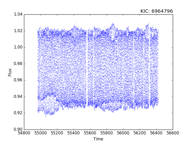
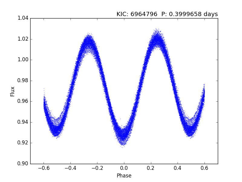
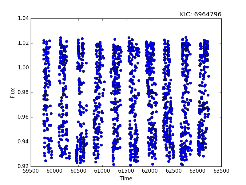
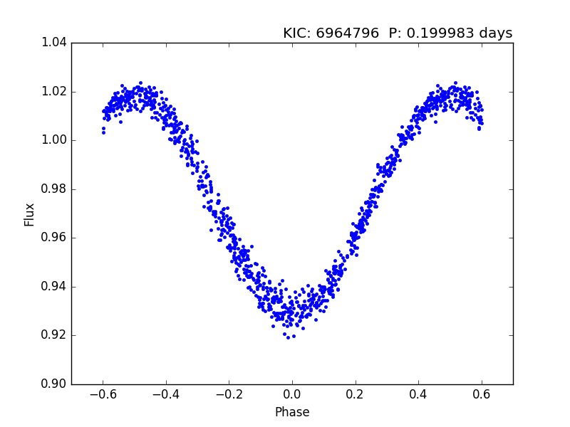
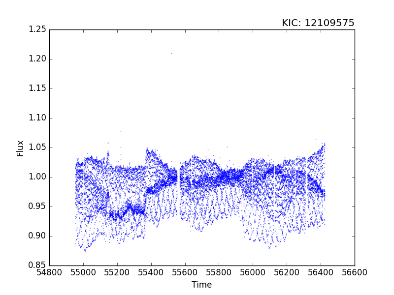
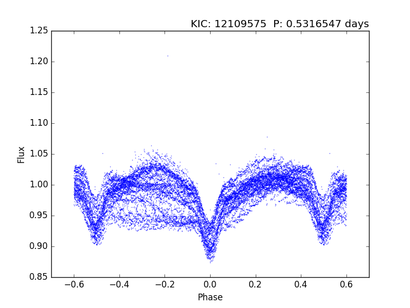
We define a successful detection (Table 2) if $P_{r}{}$ is within a specified tolerance range of one of three target values: 0.5, 1, and 2. We determined that a tolerance of 0.1% was sufficient as increasing the tolerance beyond this point did not alter the results significantly (Table 3). The values of $P_{r}{}$ were chosen because they correspond to different light curve shapes. A $P_{r}{}$ of 0.5 corresponds to the half cycle of the binary. This is the tendency if the primary and secondary eclipses are similar in shape and depth. Figure 4 shows an example of one such target. A $P_{r}{}$ of 1 indicates that the period finder returned the close-to-true orbital period of the binary. In contrast to the previous case, binaries with eclipses that are different depths and shapes have a strong orbital period signal. Figure 2 depicts a source in which the original binary period was recovered. A $P_{r}{}$ of 2 corresponds to twice the period of the binary. Spots can change the depths of the eclipses from orbit to orbit. This effect can produce light curves where the strongest period is a multiple of the orbital period of the binary. For this work we do not consider binaries with a $P_{r}{}$ greater than 2 times the orbital period. Figure 5 shows an example of a binary with a $P_{r}$ of 2.

if	$0.5(1-tol/2)\leq P_{r}\leq 0.5(1+tol/2)$	then	half-period was recovered
if	$1.0(1-tol/2)\leq P_{r}\leq 1.0(1+tol/2)$	then	period was recovered
if	$2.0(1-tol/2)\leq P_{r}\leq 2.0(1+tol/2)$	then	twice-period was recovered

Table 2: A recovery is successful if its $P_{r}{}$ is within some tolerance of the detection criterion. For example, a 1% tolerance value would give ranges of size 0.005, 0.01, and 0.02 for $P_{r}{}$ values of 0.5, 1.0, and 2.0, respectively. The criterion ranges would then be 0.49975 to 0.50025, 0.995 to 1.005, and 1.99 to 2.01, respectively.

Figure 4: Top Left: Original Kepler light curve. Top Right: The light curve phase-folded over the KEBC period. Bottom Left: LSST simulated light curve. Bottom Right: The light curve phase-folded over the AoV period.

Figure 5: Top Left: Original Kepler light curve. Top Right: The light curve phase-folded over the KEBC period. Bottom Left: LSST simulated light curve. Bottom Right: The light curve phase-folded over the AoV period.

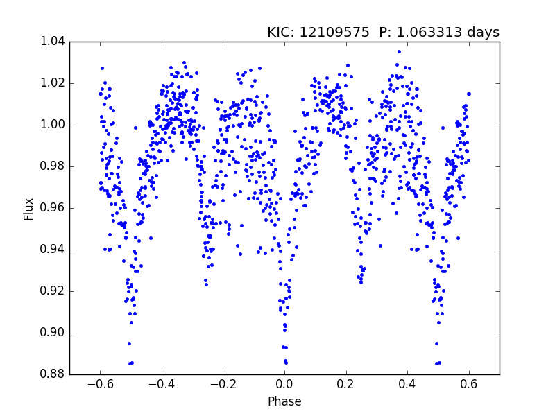The period finder successfully recovered 2027 out of the simulated 2844 binaries, 71.3% of the sample. Breaking this up into their detection types (see Table 2), we find that 1133 (39.8%) were identified by their half cycle signal and 887 (31.3%) by the true binary period. There were 7 (0.2%) that were detected with a $P_{r}{}$ of 2. These results are listed in Table 3.

	0.01%		0.02%		0.05%		0.1%		0.2%		0.5%		1.0%
$P_{r}{}$	num.	perc.	num.	perc.	num.	perc.	num.	perc.	num.	perc.	num.	perc.	num.	perc.
0.5	1066	37.48	1120	39.38	1140	40.08	1142	40.15	1142	40.15	1142	40.15	1142	40.15
	1009	35.48	1058	37.20	1074	37.76	1076	37.83	1076	37.83	1076	37.83	1076	37.83
1.0	796	27.99	860	30.24	878	30.87	879	30.91	879	30.91	879	30.91	879	30.91
	763	26.83	814	28.62	832	29.25	832	29.25	832	29.25	832	29.25	832	29.25
2.0	7	0.25	8	0.28	8	0.28	8	0.28	8	0.28	8	0.28	8	0.28
	11	0.39	11	0.39	11	0.39	11	0.39	11	0.39	11	0.39	11	0.39
success	1869	65.72	1988	69.90	2026	71.24	2029	71.34	2029	71.34	2029	71.34	2029	71.34
	1783	62.69	1883	66.21	1917	67.41	1919	67.48	1919	67.48	1919	67.48	1919	67.48
failure	975	34.28	856	30.10	818	28.76	815	28.66	815	28.66	815	28.66	815	28.66
	1061	37.31	961	33.79	927	32.59	925	32.52	925	32.52	925	32.52	925	32.52

Table 3: Results of the period detection using a variety of tolerance values. The italicized rows are the results for the light curves with the injected $5\sigma$ noise. A tolerance of 0.1% is sufficient as further increasing the tolerance does not alter the detection rates.

5 Discussion

Table 3 shows that 71.3% of the binaries were recovered with the detection of the half-period being the most common. In addition, we also looked at how the binary period impacted detection success. Figure 6 shows that, as expected, higher periods are detected less reliably.

Figure 6: The recovery rate, given as a fraction, as a function of the $P_{KEBC}{}$. In blue are the results for the light curves with $5\sigma$ noise introduced while the results for the light curves with no additional noise are in gray. For periods less than 2 days we recover nearly 100% of the binaries. The recovery success drops below 50% for binaries with periods greater than 10 days.

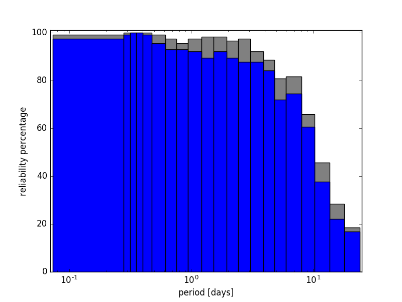The recovery rate drops below 50% for binaries with periods of above 10 days. It is also clear from the plot that the introduction of the $5\sigma$ noise suppresses the recovery rate. As expected, the suppression is period-dependent, because the geometric selection effect suppresses the detection of high eclipse amplitude light curves. The probability of an eclipse drops rapidly as the separation between components increases, which in turn means that we should expect suppression in high-amplitude light curves at the long period end. Because long period binaries will produce fewer eclipses as compared to short period binaries over the survey lifetime, the eclipse signal-to-noise ratio will be inherently lower for longer period binaries.

Figure 7 shows the number of binaries as a function of period in the KEBC. There are a substantial number of binaries to simulate even at periods of 100 days.

Figure 7: The number of binaries in the KEBC as a function of their period. The gradual drop off at higher periods is due to the geometrical probability of eclipses as well as Kepler’s duty cycle [Kirk et al., 2016].

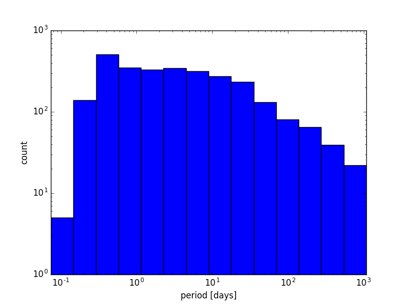
It is not surprising that binaries with shorter periods will be detected more reliably. Shorter period binaries will have their eclipses more completely sampled, allowing for a more reliable detection.

We explored what effect dithering would have on our results and there was no appreciable difference. Dithering refers to the intentional offset the scan pattern LSST will make when returning to observe the same fields. In order to get full sky coverage, LSST will have to have overlapping regions. Dithering will help smear the overlap so that coverage is more uniform.

6 Future Work

This work is a first step in the creation of a robust science metric for use in the determination of the LSST cadence algorithm. Future steps include modifying the fluxes to be more representative of what LSST would observe. Currently, the process is using Kepler fluxes without any modification.

Using simulated instead of Kepler light curves and maintaining a standard number of light curves as a function of period would help remove potential biases due to Kepler’s selection effects. Longer period binaries suffer from an intrinsic bias due to the geometric probability of eclipse detection.

Finally, constructing a light curve sample from a model of the Galaxy would allow us to evaluate the performance of LSST as a function of position beyond just the Kepler field. This model would be generated using Galaxia [Sharma et al., 2011] which implements the Besancon model [Robin et al., 2003]. The model would also consider effects from crowding near the galactic plane as well as differences in stellar density, providing (within the accuracy of the Galaxy model) a more accurate representation of the observations LSST will be making.

References

- Abdul-Masih et al. [2016] M. Abdul-Masih, A. Prša, K. Conroy, S. Bloemen, T. Boyajian, L. R. Doyle, C. Johnston, V. Kostov, D. W. Latham, G. Matijevič, A. Shporer, and J. Southworth. Kepler Eclipsing Binary Stars. VIII. Identification of False Positive Eclipsing Binaries and Re-extraction of New Light Curves. AJ, 151:101, Apr. 2016. 10.3847/0004-6256/151/4/101.
- Allen et al. [2007] P. R. Allen, D. W. Koerner, M. W. McElwain, K. L. Cruz, and I. N. Reid. A New Brown Dwarf Desert? A Scarcity of Wide Ultracool Binaries. AJ, 133(3):971, 2007. URL http://stacks.iop.org/1538-3881/133/i=3/a=971.
- Astropy Collaboration et al. [2013] Astropy Collaboration, T. P. Robitaille, E. J. Tollerud, P. Greenfield, M. Droettboom, E. Bray, T. Aldcroft, M. Davis, A. Ginsburg, A. M. Price-Whelan, W. E. Kerzendorf, A. Conley, N. Crighton, K. Barbary, D. Muna, H. Ferguson, F. Grollier, M. M. Parikh, P. H. Nair, H. M. Unther, C. Deil, J. Woillez, S. Conseil, R. Kramer, J. E. H. Turner, L. Singer, R. Fox, B. A. Weaver, V. Zabalza, Z. I. Edwards, K. Azalee Bostroem, D. J. Burke, A. R. Casey, S. M. Crawford, N. Dencheva, J. Ely, T. Jenness, K. Labrie, P. L. Lim, F. Pierfederici, A. Pontzen, A. Ptak, B. Refsdal, M. Servillat, and O. Streicher. Astropy: A community Python package for astronomy. A&A, 558:A33, Oct. 2013. 10.1051/0004-6361/201322068.
- Borucki et al. [2010] W. J. Borucki, D. Koch, G. Basri, N. Batalha, T. Brown, D. Caldwell, J. Caldwell, J. Christensen-Dalsgaard, W. D. Cochran, E. DeVore, E. W. Dunham, A. K. Dupree, T. N. Gautier, J. C. Geary, R. Gilliland, A. Gould, S. B. Howell, J. M. Jenkins, Y. Kondo, D. W. Latham, G. W. Marcy, S. Meibom, H. Kjeldsen, J. J. Lissauer, D. G. Monet, D. Morrison, D. Sasselov, J. Tarter, A. Boss, D. Brownlee, T. Owen, D. Buzasi, D. Charbonneau, L. Doyle, J. Fortney, E. B. Ford, M. J. Holman, S. Seager, J. H. Steffen, W. F. Welsh, J. Rowe, H. Anderson, L. Buchhave, D. Ciardi, L. Walkowicz, W. Sherry, E. Horch, H. Isaacson, M. E. Everett, D. Fischer, G. Torres, J. A. Johnson, M. Endl, P. MacQueen, S. T. Bryson, J. Dotson, M. Haas, J. Kolodziejczak, J. Van Cleve, H. Chandrasekaran, J. D. Twicken, E. V. Quintana, B. D. Clarke, C. Allen, J. Li, H. Wu, P. Tenenbaum, E. Verner, F. Bruhweiler, J. Barnes, and A. Prsa. Kepler planet-detection mission: Introduction and first results. Science, 327(5968):977–980, 2010. ISSN 0036-8075. 10.1126/science.1185402. URL http://science.sciencemag.org/content/327/5968/977.
- Burgasser et al. [2003] A. J. Burgasser, J. D. Kirkpatrick, I. N. Reid, M. E. Brown, C. L. Miskey, and J. E. Gizis. Binarity in Brown Dwarfs: T Dwarf Binaries Discovered with the Hubble Space Telescope Wide Field Planetary Camera 2. ApJ, 586:512–526, Mar. 2003. 10.1086/346263.
- Christiansen et al. [2012] J. L. Christiansen, J. M. Jenkins, D. A. Caldwell, C. J. Burke, P. Tenenbaum, S. Seader, S. E. Thompson, T. S. Barclay, B. D. Clarke, J. Li, J. C. Smith, M. C. Stumpe, J. D. Twicken, and J. Van Cleve. The Derivation, Properties, and Value of Kepler’s Combined Differential Photometric Precision. PASP, 124:1279–1287, Dec. 2012. 10.1086/668847.
- Connolly et al. [2014] A. J. Connolly, G. Z. Angeli, S. Chandrasekharan, C. F. Claver, K. Cook, Z. Ivezic, R. L. Jones, K. S. Krughoff, E.-H. Peng, J. Peterson, C. Petry, A. P. Rasmussen, S. T. Ridgway, A. Saha, G. Sembroski, J. vanderPlas, and P. Yoachim. An end-to-end simulation framework for the large synoptic survey telescope, 2014. URL http://dx.doi.org/10.1117/12.2054953.
- Delgado et al. [2014] F. Delgado, A. Saha, S. Chandrasekharan, K. Cook, C. Petry, and S. Ridgway. The LSST operations simulator. In Modeling, Systems Engineering, and Project Management for Astronomy VI, volume 9150 of Proc. SPIE, page 915015, Aug. 2014. 10.1117/12.2056898.
- Devor [2005] J. Devor. Solutions for 10,000 Eclipsing Binaries in the Bulge Fields of OGLE II Using DEBiL. ApJ, 628:411–425, July 2005. 10.1086/431170.
- Fischer and Marcy [1992] D. A. Fischer and G. W. Marcy. Multiplicity among M dwarfs. ApJ, 396:178–194, Sept. 1992. 10.1086/171708.
- Hartman and Bakos [2016] J. D. Hartman and G. Á. Bakos. VARTOOLS: A program for analyzing astronomical time-series data. Astronomy and Computing, 17:1–72, Oct. 2016. 10.1016/j.ascom.2016.05.006.
- Henry and McCarthy [1990] T. J. Henry and D. W. McCarthy, Jr. A systematic search for brown dwarfs orbiting nearby stars. ApJ, 350:334–347, Feb. 1990. 10.1086/168387.
- Ivezić et al. [2008] Z. Ivezić, J. A. Tyson, B. Abel, E. Acosta, R. Allsman, Y. AlSayyad, S. F. Anderson, J. Andrew, R. Angel, G. Angeli, R. Ansari, P. Antilogus, K. T. Arndt, P. Astier, E. Aubourg, T. Axelrod, D. J. Bard, J. D. Barr, A. Barrau, J. G. Bartlett, B. J. Bauman, S. Beaumont, A. C. Becker, J. Becla, C. Beldica, S. Bellavia, G. Blanc, R. D. Blandford, J. S. Bloom, J. Bogart, K. Borne, J. F. Bosch, D. Boutigny, W. N. Brandt, M. E. Brown, J. S. Bullock, P. Burchat, D. L. Burke, G. Cagnoli, D. Calabrese, S. Chandrasekharan, S. Chesley, E. C. Cheu, J. Chiang, C. F. Claver, A. J. Connolly, K. H. Cook, A. Cooray, K. R. Covey, C. Cribbs, W. Cui, R. Cutri, G. Daubard, G. Daues, F. Delgado, S. Digel, P. Doherty, R. Dubois, G. P. Dubois-Felsmann, J. Durech, M. Eracleous, H. Ferguson, J. Frank, M. Freemon, E. Gangler, E. Gawiser, J. C. Geary, P. Gee, M. Geha, R. R. Gibson, D. K. Gilmore, T. Glanzman, I. Goodenow, W. J. Gressler, P. Gris, A. Guyonnet, P. A. Hascall, J. Haupt, F. Hernandez, C. Hogan, D. Huang, M. E. Huffer, W. R. Innes, S. H. Jacoby, B. Jain, J. Jee, J. G. Jernigan, D. Jevremovic, K. Johns, R. L. Jones, C. Juramy-Gilles, M. Juric, S. M. Kahn, J. S. Kalirai, N. Kallivayalil, B. Kalmbach, J. P. Kantor, M. M. Kasliwal, R. Kessler, D. Kirkby, L. Knox, I. Kotov, V. L. Krabbendam, S. Krughoff, P. Kubanek, J. Kuczewski, S. Kulkarni, R. Lambert, L. Le Guillou, D. Levine, M. Liang, K. Lim, C. Lintott, R. H. Lupton, A. Mahabal, P. Marshall, S. Marshall, M. May, R. McKercher, M. Migliore, M. Miller, D. J. Mills, D. G. Monet, M. Moniez, D. R. Neill, J. Nief, A. Nomerotski, M. Nordby, P. O’Connor, J. Oliver, S. S. Olivier, K. Olsen, S. Ortiz, R. E. Owen, R. Pain, J. R. Peterson, C. E. Petry, F. Pierfederici, S. Pietrowicz, R. Pike, P. A. Pinto, R. Plante, S. Plate, P. A. Price, M. Prouza, V. Radeka, J. Rajagopal, A. Rasmussen, N. Regnault, S. T. Ridgway, S. Ritz, W. Rosing, C. Roucelle, M. R. Rumore, S. Russo, A. Saha, B. Sassolas, T. L. Schalk, R. H. Schindler, D. P. Schneider, G. Schumacher, J. Sebag, G. H. Sembroski, L. G. Seppala, I. Shipsey, N. Silvestri, J. A. Smith, R. C. Smith, M. A. Strauss, C. W. Stubbs, D. Sweeney, A. Szalay, P. Takacs, J. J. Thaler, R. Van Berg, D. Vanden Berk, K. Vetter, F. Virieux, B. Xin, L. Walkowicz, C. W. Walter, D. L. Wang, M. Warner, B. Willman, D. Wittman, S. C. Wolff, W. M. Wood-Vasey, P. Yoachim, H. Zhan, and for the LSST Collaboration. LSST: from Science Drivers to Reference Design and Anticipated Data Products. ArXiv e-prints, May 2008.
- Jenkins et al. [2010] J. M. Jenkins, H. Chandrasekaran, S. D. McCauliff, D. A. Caldwell, P. Tenenbaum, J. Li, T. C. Klaus, M. T. Cote, and C. Middour. Transiting planet search in the kepler pipeline, 2010. URL http://dx.doi.org/10.1117/12.856764.
- Joergens [2008] V. Joergens. Binary frequency of very young brown dwarfs at separations smaller than 3 AU. A&A, 492(2):545–555, 2008. 10.1051/0004-6361:200810413. URL http://dx.doi.org/10.1051/0004-6361:200810413.
- Jones et al. [2014] R. L. Jones, P. Yoachim, S. Chandrasekharan, A. J. Connolly, K. H. Cook, . Ivezić, K. S. Krughoff, C. Petry, and S. T. Ridgway. The LSST metrics analysis framework (MAF). Proc. SPIE, 9149:91490B–91490B–18, 2014. 10.1117/12.2056835. URL http://dx.doi.org/10.1117/12.2056835.
- Kirk et al. [2016] B. Kirk, K. Conroy, A. Prša, M. Abdul-Masih, A. Kochoska, G. Matijevič, K. Hambleton, T. Barclay, S. Bloemen, T. Boyajian, L. R. Doyle, B. J. Fulton, A. J. Hoekstra, K. Jek, S. R. Kane, V. Kostov, D. Latham, T. Mazeh, J. A. Orosz, J. Pepper, B. Quarles, D. Ragozzine, A. Shporer, J. Southworth, K. Stassun, S. E. Thompson, W. F. Welsh, E. Agol, A. Derekas, J. Devor, D. Fischer, G. Green, J. Gropp, T. Jacobs, C. Johnston, D. M. LaCourse, K. Saetre, H. Schwengeler, J. Toczyski, G. Werner, M. Garrett, J. Gore, A. O. Martinez, I. Spitzer, J. Stevick, P. C. Thomadis, E. H. Vrijmoet, M. Yenawine, N. Batalha, and W. Borucki. Kepler Eclipsing Binary Stars. VII. The Catalog of Eclipsing Binaries Found in the Entire Kepler Data Set. AJ, 151:68, Mar. 2016. 10.3847/0004-6256/151/3/68.
- Kobulnicky and Fryer [2007] H. A. Kobulnicky and C. L. Fryer. A New Look at the Binary Characteristics of Massive Stars. ApJ, 670:747–765, Nov. 2007. 10.1086/522073.
- Kouwenhoven et al. [2007] M. B. N. Kouwenhoven, A. G. A. Brown, S. F. Portegies Zwart, and L. Kaper. The primordial binary population. II.. Recovering the binary population for intermediate mass stars in Scorpius OB2. A&A, 474:77–104, Oct. 2007. 10.1051/0004-6361:20077719.
- LSST Science Collaboration et al. [2009] LSST Science Collaboration, P. A. Abell, J. Allison, S. F. Anderson, J. R. Andrew, J. R. P. Angel, L. Armus, D. Arnett, S. J. Asztalos, T. S. Axelrod, and et al. LSST Science Book, Version 2.0. ArXiv e-prints, Dec. 2009.
- Mason et al. [1998] B. D. Mason, D. R. Gies, W. I. Hartkopf, W. G. Bagnuolo, Jr., T. ten Brummelaar, and H. A. McAlister. ICCD speckle observations of binary stars. XIX - an astrometric/spectroscopic survey of O stars. AJ, 115:821, Feb. 1998. 10.1086/300234.
- Mason et al. [2009] B. D. Mason, W. I. Hartkopf, D. R. Gies, T. J. Henry, and J. W. Helsel. The High Angular Resolution Multiplicity of Massive Stars. AJ, 137:3358–3377, Feb. 2009. 10.1088/0004-6256/137/2/3358.
- Maxted et al. [2008] P. F. L. Maxted, R. D. Jeffries, J. M. Oliveira, T. Naylor, and R. J. Jackson. A survey for low-mass spectroscopic binary stars in the young clusters around Orionis and Orionis. MNRAS, 385(4):2210–2224, 2008. 10.1111/j.1365-2966.2008.13008.x. URL http://mnras.oxfordjournals.org/content/385/4/2210.abstract.
- Pont et al. [2006] F. Pont, S. Zucker, and D. Queloz. The effect of red noise on planetary transit detection. Monthly Notices of the Royal Astronomical Society, 373(1):231, 2006. 10.1111/j.1365-2966.2006.11012.x. URL +http://dx.doi.org/10.1111/j.1365-2966.2006.11012.x.
- Prša et al. [2011] A. Prša, N. Batalha, R. W. Slawson, L. R. Doyle, W. F. Welsh, J. A. Orosz, S. Seager, M. Rucker, K. Mjaseth, S. G. Engle, K. Conroy, J. Jenkins, D. Caldwell, D. Koch, and W. Borucki. Kepler Eclipsing Binary Stars. I. Catalog and Principal Characterization of 1879 Eclipsing Binaries in the First Data Release. AJ, 141:83, Mar. 2011. 10.1088/0004-6256/141/3/83.
- Raghavan et al. [2010] D. Raghavan, H. A. McAlister, T. J. Henry, D. W. Latham, G. W. Marcy, B. D. Mason, D. R. Gies, R. J. White, and T. A. ten Brummelaar. A Survey of Stellar Families: Multiplicity of Solar-type Stars. ApJS, 190:1–42, Sept. 2010. 10.1088/0067-0049/190/1/1.
- Reid and Gizis [1997] I. N. Reid and J. E. Gizis. Low-Mass Binaries in the Hyades: A Scarcity of Brown Dwarfs. AJ, 114:1992, Nov. 1997. 10.1086/118620.
- Ribas et al. [2005] I. Ribas, C. Jordi, F. Vilardell, E. L. Fitzpatrick, R. W. Hilditch, and E. F. Guinan. First Determination of the Distance and Fundamental Properties of an Eclipsing Binary in the Andromeda Galaxy. ApJ, 635:L37–L40, Dec. 2005. 10.1086/499161.
- Robin et al. [2003] A. C. Robin, C. Reylé, S. Derrière, and S. Picaud. A synthetic view on structure and evolution of the Milky Way. A&A, 409:523–540, Oct. 2003. 10.1051/0004-6361:20031117.
- Schwarzenberg-Czerny [1989] A. Schwarzenberg-Czerny. On the advantage of using analysis of variance for period search. MNRAS, 241:153–165, Nov. 1989. 10.1093/mnras/241.2.153.
- Sharma et al. [2011] S. Sharma, J. Bland-Hawthorn, K. V. Johnston, and J. Binney. Galaxia: A Code to Generate a Synthetic Survey of the Milky Way. ApJ, 730:3, Mar. 2011. 10.1088/0004-637X/730/1/3.
- Shatsky and Tokovinin [2002] N. Shatsky and A. Tokovinin. The mass ratio distribution of B-type visual binaries in the Sco OB2 association. A&A, 382:92–103, Jan. 2002. 10.1051/0004-6361:20011542.
- Siegler et al. [2005] N. Siegler, L. M. Close, K. L. Cruz, E. L. Martín, and I. N. Reid. Discovery of Two Very Low Mass Binaries: Final Results of an Adaptive Optics Survey of Nearby M6.0-M7.5 Stars. ApJ, 621:1023–1032, Mar. 2005. 10.1086/427743.
- Slawson et al. [2011] R. W. Slawson, A. Prša, W. F. Welsh, J. A. Orosz, M. Rucker, N. Batalha, L. R. Doyle, S. G. Engle, K. Conroy, J. Coughlin, T. A. Gregg, T. Fetherolf, D. R. Short, G. Windmiller, D. C. Fabrycky, S. B. Howell, J. M. Jenkins, K. Uddin, F. Mullally, S. E. Seader, S. E. Thompson, D. T. Sanderfer, W. Borucki, and D. Koch. Kepler Eclipsing Binary Stars. II. 2165 Eclipsing Binaries in the Second Data Release. AJ, 142:160, Nov. 2011. 10.1088/0004-6256/142/5/160.
- Tange [2011] O. Tange. Gnu parallel - the command-line power tool. ;login: The USENIX Magazine, 36(1):42–47, Feb 2011. URL http://www.gnu.org/s/parallel.
- Tenenbaum et al. [2012] P. Tenenbaum, J. L. Christiansen, J. M. Jenkins, J. F. Rowe, S. Seader, D. A. Caldwell, B. D. Clarke, J. Li, E. V. Quintana, J. C. Smith, M. C. Stumpe, S. E. Thompson, J. D. Twicken, J. V. Cleve, W. J. Borucki, M. T. Cote, M. R. Haas, D. T. Sanderfer, F. R. Girouard, T. C. Klaus, C. K. Middour, B. Wohler, N. M. Batalha, T. Barclay, and J. E. Nickerson. Detection of potential transit signals in the first three quarters of kepler mission data. The Astrophysical Journal Supplement Series, 199(1):24, 2012. URL http://stacks.iop.org/0067-0049/199/i=1/a=24.
- Torres et al. [2010] G. Torres, J. Andersen, and A. Giménez. Accurate masses and radii of normal stars: modern results and applications. A&A Rev., 18:67–126, Feb. 2010. 10.1007/s00159-009-0025-1.
- Van Cleve and Caldwell [2009] J. Van Cleve and D. A. Caldwell. Kepler Instrument Handbook, KSCI 19033-001, 2009.