Testing invisible momentum ansatze in missing energy events at the LHC

Abstract

We consider SUSY-like events with two decay chains, each terminating in an invisible particle, whose true energy and momentum are not measured in the detector. Nevertheless, a useful educated guess about the invisible momenta can still be obtained by optimizing a suitable invariant mass function. We review and contrast several proposals in the literature for such ansatze: four versions of the $M_{T2}$-assisted on-shell reconstruction (MAOS), as well as several variants of the on-shell constrained $M_{2}$ variables. We compare the performance of these methods with regards to the mass determination of a new particle resonance along the decay chain from the peak of the reconstructed invariant mass distribution. For concreteness, we consider the event topology of dilepton $t\bar{t}$ events and study each of the three possible subsystems, in both a $t\bar{t}$ and a SUSY example. We find that the $M_{2}$ variables generally provide sharper peaks and therefore better ansatze for the invisible momenta. We show that the performance can be further improved by preselecting events near the kinematic endpoint of the corresponding variable from which the momentum ansatz originates.

1 Introduction

The bread and butter method for discovering a new particle in high energy physics is the “bump hunt”: one identifies and measures the momenta and energies of all relevant decay products, and forms their total invariant mass. Signal events, which are due to the production of a new resonance, appear as a localized “bump” feature over the relatively smooth background continuum. This technique has led to many discoveries in the past, including the most recent discovery of the Standard Model Higgs boson, which was first observed as an invariant mass peak in the four-lepton and di-photon channels Chatrchyan:2012xdj ; Aad:2012tfa .

However, this tried and true method faces a major challenge when one (or more) of the decay products are neutral, weakly interacting particles, which are invisible in the detector, and as a result their energies and momenta remain unknown. Many well-motivated models of new physics Beyond the Standard Model (BSM) contain such particles, as they are the prototypical dark matter candidates. Consequently, one has to develop alternative methods for discovery (and mass measurement) which are applicable to the case of such semi-invisible resonance decays.

The situation is further complicated by the fact that most BSM models with dark matter candidates introduce a conserved discrete symmetry, often a $Z_{2}$ parity, in order to protect the lifetime of the dark matter particle. The new particles which are charged under this symmetry are necessarily pair produced; therefore, each event contains not one, but at least two invisible (dark matter) particles whose 4-momenta $q_{1}^{\mu}$ and $q_{2}^{\mu}$ are not individually measured. At hadron colliders, it is only the sum $\vec{q}_{1T}+\vec{q}_{2T}$ of their transverse momenta which can be measured in the form of the missing transverse momentum ${\;/\!\!\!\!\vec{P}_{T}}$ of the event:

$$\vec{q}_{1T}+\vec{q}_{2T}={\;/\!\!\!\!\vec{P}_{T}}.$$ (1)

However, the partitioning of the measured ${\;/\!\!\!\!\vec{P}_{T}}$ into $\vec{q}_{1T}$ and $\vec{q}_{2T}$ is a priori unknown, and furthermore, the longitudinal components $q_{1z}$ and $q_{2z}$ remain arbitrary at this point as well.

Over the last 15-20 years, a large number of methods have been proposed to deal with measurements in such “SUSY-like” events, i.e., events with two decay chains, each terminating in an invisible particle (see Ref. Barr:2010zj for a recent review). One possibility is to try to calculate exactly the unknown individual 4-momenta $q_{i}^{\mu}$ of the invisible particles, which in turn would allow one to reconstruct an invariant mass peak again. Unfortunately, this idea can only be applied to very specific event topologies, where the decay chains are sufficiently long, yielding enough mass-shell constraints in addition to (1) Kawagoe:2004rz ; Nojiri:2007pq ; Cheng:2008mg ; Cheng:2009fw . This is why the majority of the proposed methods have abandoned the idea of directly measuring a mass peak, and instead focused on measuring a kinematic endpoint for a suitably defined variable.

Now, what constitutes a “good” kinematic variable for a kinematic endpoint measurement? The answer to this question in principle depends on several factors, including the assumed event topology, the nature of the visible SM particles in the final state, the precision with which their momenta $p_{j}$ are measured, etc. Roughly speaking, we can divide the set of kinematic variables into two categories:

• Variables built only from directly measured quantities, i.e., the momenta $p_{j}$ of the visible final state particles and the missing transverse momentum ${\;/\!\!\!\!\vec{P}_{T}}$. The primary example of such a variable is the invariant mass of a collection of visible particles. This idea forms the basis of the classic method for mass determination in supersymmetry from kinematic endpoints Hinchliffe:1996iu ; Bachacou:1999zb ; Allanach:2000kt ; Gjelsten:2004ki ; Gjelsten:2005aw ; Matchev:2009iw ; Kim:2015bnd . Other variables belonging to this class include the scalar sum $H_{T}$ of the transverse momenta of visible objects (jets or leptons), the effective mass $M_{eff}$ Hinchliffe:1996iu ; Tovey:2000wk , the contransverse mass variable $M_{CT}$ Tovey:2008ui ; Polesello:2009rn and its variants $M_{CT_{\perp}}$ and $M_{CT_{\parallel}}$ Matchev:2009ad , the ratio of visible transverse energies Nojiri:2000wq ; Cheng:2011ya , and the energy itself Agashe:2012bn ; Agashe:2012fs ; Agashe:2013eba ; Chen:2014oha ; Agashe:2015wwa ; Agashe:2015ike . The advantage of these variables is their simplicity, since one does not have to even face the question about the individual momenta $q_{i}$ or masses $\tilde{m}_{i}$ of the invisible particles in the event. In principle, these variables are very general and can be usefully applied in certain situations; however, they also fail to take advantage of the specific characteristics of the event, and become suboptimal for more complex event topologies.

• Variables defined in terms of both the measured momenta $p_{j}$ and the invisible momenta $q_{i}$. Of course, since the individual invisible momenta $q_{i}$ are unknown, the definition of any such variable

  $$v\equiv v(p_{j},q_{i})$$ (2)

  must be supplemented with a procedure for fixing the values of the invisible momenta $q_{i}$ through a suitable ansatz. More concretely, the ansatz should allow us to compute the invisible 4-momenta $q_{i}^{\mu}$ in terms of the measured visible 4-momenta $p_{j}^{\nu}$ and a set of hypothesized masses $\tilde{m}_{i}$ for the invisible particles:

  $$q_{i}^{\mu}=q_{i}^{\mu}(p_{j}^{\nu},\tilde{m}_{i}),$$ (3)

  so that at the end of the day, the kinematic variable (2) can be equivalently expressed in terms of visible momenta $p_{j}$ and invisible masses $\tilde{m}_{i}$ only:

  $$v=v(p_{j},q_{i}(p_{j},\tilde{m}_{i})).$$ (4)

  If one is solely interested in the kinematic variable $v$ itself and its properties (differential distribution, kinematic endpoints, etc.), the intermediate step (3) of computing the individual invisible momenta $q_{i}$ is unimportant and can be regarded simply as a convenient calculational tool. In fact, many of the computer codes on the market which are used to compute kinematic variables of the type (2), by default do not even report the values for the invisible momenta found from the ansatz (3). There are also some special cases, e.g., the minimum partonic center-of-mass energy $\sqrt{\hat{s}}_{min}$ Konar:2008ei ; Robens:2011zm , the razor variables Rogan:2010kb ; Buckley:2013kua , or the transverse mass $M_{T}$ Smith:1983aa ; Barger:1983wf , where one can solve for the ansatz (3) analytically, eliminate the invisible momenta, and derive an exact analytical expression for the variable $v$ in the form of (4), which can then serve as an alternative definition, without reference to any invisible momenta at all.

  Perhaps the two best known examples of variables of the type (2) are the transverse mass Smith:1983aa ; Barger:1983wf and the Cambridge $M_{T2}$ variable Lester:1999tx ; Barr:2003rg . Recently this set of variables was expanded significantly and now includes $M_{T2\perp}$ and $M_{T2\parallel}$ Konar:2009wn , the asymmetric $M_{T2}$ Barr:2009jv ; Konar:2009qr , $M_{2C}$ Ross:2007rm ; Barr:2008ba , $M_{CT2}$ Cho:2009ve ; Cho:2010vz , $M_{T2}^{approx}$ Lally:2012uj , and the constrained $M_{2}$ variables Mahbubani:2012kx ; Cho:2014naa ; Cho:2014yma ; Kim:2014ana ; Cho:2015laa . As the index $``2"$ suggests, all these variables were designed for the case of SUSY-like events with two decay chains, and they also carry an implicit dependence on the test masses $\tilde{m}_{i}$ of the invisible particles, as indicated in (4). Despite the large number of such variables on the market, they all share the same common idea Barr:2011xt : choose a suitable target function and minimize it over all possible values of the individual invisible momenta $q_{i}$ which are consistent with the ${\;/\!\!\!\!\vec{P}_{T}}$ condition (1). The variations arise because one faces a menu of choices:

  • Partitioning of the event. One groups the final state particles according to the assumed production process — single production, pair production, etc. Ideally, one should also have a separate category for jets which are suspected to come from initial state radiation Lester:2007fq ; Papaefstathiou:2009hp ; Alwall:2009zu ; Konar:2010ma .

  • Choice of target function. The target function can be a full (3+1)-dimensional invariant mass, as in the case of $\sqrt{\hat{s}}_{min}$ Konar:2008ei , $M_{2C}$ Ross:2007rm ; Barr:2008ba and $M_{2}$ Mahbubani:2012kx ; Cho:2014naa ; a (2+1)-dimensional transverse mass, e.g., $M_{T}$ Smith:1983aa ; Barger:1983wf or $M_{T2}$ Lester:1999tx , and even a (1+1)-dimensional mass as in the case of $M_{T2\perp}$ and $M_{T2\parallel}$ Konar:2009wn . Note that the projection to lower dimensions in general does not commute with the partitioning, so by performing those two operations in different order, one obtains in principle different variables Barr:2011xt .

  • Imposing additional on-shell constraints. The minimization of (3+1)-dimensional mass target functions over the invisible momenta can be performed by taking into account the ${\;/\!\!\!\!\vec{P}_{T}}$ constraint (1) only, or by adding additional kinematic constraints which are motivated by the assumed event topology Mahbubani:2012kx ; Cho:2014naa ; Swain:2014dha ; Konar:2015hea , a prior kinematic endpoint measurement Ross:2007rm , or by the presence of a known SM particle in the decay chain (for example, a $W$ boson Barr:2011ux ; Barr:2011si ; Bai:2012gs ; Swain:2014dha or a $\tau$ lepton Barr:2011he ; Swain:2014dha ; Konar:2016wbh ). The additional on-shell constraints further restrict the allowed domain of values for the components of the individual invisible momenta $q_{i}$ and in general lead to a different outcome from the minimization procedure.

  Note that whenever the target function is a transverse mass in (2+1) dimensions, the minimization fixes only the transverse components $\vec{q}_{iT}$ of the invisible momenta, and for the longitudinal components one must rely on additional measurements or assumptions. For example, in the $M_{T2}$-assisted on-shell (MAOS) reconstruction method, one assumes knowledge of the mass of the mother particle and enforces its on-shell condition, which allows to solve for the longitudinal momenta Cho:2008tj . The method was then tested in examples where the mothers are known SM particles, e.g. top quarks, $W$-bosons or $\tau$-leptons Choi:2009hn ; Cho:2009wh ; Park:2011uz ; Choi:2010dw ; Choi:2011ys ; Guadagnoli:2013xia . Since the on-shell constraints are nonlinear functions, the MAOS approach typically yields multiple solutions for the longitudinal momentum components, so one must also specify a prescription for handling this multiplicity. In contrast, target functions defined in (3+1) dimensions automatically yield ansatze for the full energy-momentum 4-vectors $q^{\mu}_{i}$, without any need for additional assumptions Barr:2011xt . Another benefit of the (3+1) formulation is that the obtained solutions for the longitudinal components $q_{iz}$ are typically unique Cho:2014naa ; Cho:2015laa .

In this paper, we would like to reemphasize the existence of various ansatze (3) for the individual invisible momenta in missing energy events, and demonstrate their utility in the context of a mass measurement through a “bump hunt”. Following previous studies, we shall consider the general event topology of dilepton $t\bar{t}$ events, which already have very rich kinematics, as one can define and study three different subsystems Burns:2008va : one associated with the two $b$-jets, another associated with the two leptons, and a third one referring to the event as a whole (see Fig. 1 below). After briefly introducing our notation and conventions in Section 2, in the next Section 3 we shall carefully define and contrast the different ansatze for invisible momenta which follow from some of the most commonly discussed in the literature variables of type (2): $M_{T2}$, $M_{2}$, and $\sqrt{\hat{s}}_{min}$. The transverse variable $M_{T2}$ is already at the heart of (as well as in the name of) the MAOS method Cho:2008tj . In addition to the traditional MAOS method described earlier, in Section 3.1 we shall also consider two modified MAOS prescriptions Choi:2009hn ; Cho:2009wh ; Park:2011uz ; Choi:2010dw , which avoid using information about the mother particle mass, and instead rely on the calculated value of $M_{T2}$ in the event. (There will also be a fourth variant of the MAOS method, which will assume a known mass for a particle other than the parent.) Then in Section 3.2 we shall consider the case of (3+1)-dimensional target functions, since it automatically provides an ansatz for the longitudinal invisible momenta Konar:2008ei ; Cho:2014naa .

Next we would like to compare the performance of the difference ansatze (3). One possibility is to compare the momenta predicted by (3) to the true invisible momenta in the event. However, the ultimate goal of any invisible momentum reconstruction is to perform some kind of physics measurement. In particular, once we have a guess for the invisible momenta, we can revisit the original idea for a bump hunt, and compare the precision of mass measurements performed with different ansatze. This will be the subject of Section 4, in which we shall study the position and the sharpness of the corresponding reconstructed invariant mass peak. Our main result will be that the invisible momenta provided by $M_{2}$-type variables generally lead to the most accurate mass measurements.

In Section 5 we shall generalize our discussion to the case of BSM collider signals exhibiting the $t\bar{t}$ event topology. In particular, we shall explore the general mass parameter space of the three particles in each decay chain, and analyze the performance of the invisible momentum reconstruction from $M_{2}$-type variables as a function of parameter space. In doing so, we shall identify the parameter space regions where the accuracy is degraded, and then propose a solution for recovering sensitivity by applying a preselection cut. The same idea has already been used successfully in the case of MAOS Cho:2008tj and here we demonstrate its validity in a more general context. Sec. 6 is reserved for our conclusions.

2 Notations and setup

In this paper we shall largely follow the notation and terminology of Ref. Cho:2014naa , which we briefly review here for the reader’s convenience.

2.1 The physics process

Figure 1: The decay topology under consideration in this paper with the corresponding three subsystems explicitly delineated. Each parent particle, $A_{i}$, ($i=1,2$) decays to two visible particles, $a_{i}$ and $b_{i}$, and an invisible daughter particle, $C_{i}$, through an intermediate on-shell resonance, $B_{i}$. The blue dotted, green dot-dashed, and black solid lines indicate the subsystems $(a)$, $(b)$, and $(ab)$, respectively.

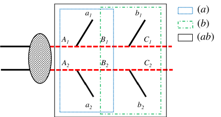
We focus on the generic event topology which is schematically depicted in Fig. 1. We assume the pair production of two heavy particles, $A_{1}$ and $A_{2}$, whose subsequent decay chains consist of two two-body decays:

$$pp\to A_{1}A_{2},\quad A_{i}\to a_{i}B_{i},\quad B_{i}\to b_{i}C_{i},\quad(i=1,2).$$ (5)

Here the particles $a_{i}$ and $b_{i}$ are SM particles which are visible in the detector, so that their 4-momenta $p_{a_{1}}^{\mu}$, $p_{b_{1}}^{\mu}$, $p_{a_{2}}^{\mu}$, and $p_{b_{2}}^{\mu}$ are measured known quantities. In contrast, the particles $C_{i}$ are invisible in the detector — they can be dark matter candidates or SM neutrinos — and their 4-momenta, $q_{i}^{\mu}$, are a priori unknown, being constrained only by the ${\;/\!\!\!\!\vec{P}_{T}}$ measurement (1) and our conjectured values $\tilde{m}_{C_{1}}$ and $\tilde{m}_{C_{2}}$ for their masses:

$$q_{i}^{2}=\tilde{m}_{C_{i}}^{2},\quad(i=1,2).$$ (6)

As usual, all visible particles are assumed massless (this is done merely for simplicity). The masses of the intermediate resonances in Fig. 1 are denoted by $m_{A_{i}}$ and $m_{B_{i}}$, with $m_{A_{i}}>m_{B_{i}}$. The process (5) depicted in Fig. 1 covers a large class of interesting and motivated scenarios, including dilepton $t\bar{t}$ events in the SM, stop pair production in supersymmetry with $\tilde{t}\to b\tilde{\chi}^{+}$, followed by $\chi^{+}\to\ell^{+}\tilde{\nu}_{\ell}$, gluino pair production in supersymmetry with $\tilde{g}\to\bar{q}\tilde{q}$, followed by $\tilde{q}\to q\tilde{\chi}^{0}$, and many more.

2.2 Event subsystems and the particle family tree nomenclature

As first discussed in the context of the $M_{T2}$ variable Burns:2008va , within the original event one can consider several useful subsystems which are delineated by the colored rectangles in Fig. 1. Each subsystem is defined by a choice of parent particles and a choice of daughter particles among the set of three particles $\left\{A_{i},B_{i},C_{i}\right\}$. Since the parents must be heavier than the daughters, there are only three possibilities, and in each case, the remaining third type of particles will be referred to as relatives. Following the notation of Cho:2014naa , we shall label each subsystem by the set of visible particles on each decay side which are used to construct the kinematic variable:

• The $(ab)$ subsystem. This system refers to the event as a whole and is indicated by the solid black box in Fig. 1. Here the $A_{i}$’s are the two parent particles and the $C_{i}$’s are the daughter particles, leaving the intermediate resonances $B_{i}$ as the relative particles. The visible particles on each side, $a_{i}$ and $b_{i}$, are combined into a composite visible particle with 4-momentum $p^{\mu}_{a_{i}}+p^{\mu}_{b_{i}}$.

• The $(b)$ subsystem. This subsystem is outlined by the green dot-dashed box in Fig. 1. Now the parents are the $B_{i}$ particles, the daughters are the $C_{i}$ particles, and the relatives are the $A_{i}$ particles. The kinematic variables for this subsystem will be defined in terms of the 4-momenta $p^{\mu}_{b_{i}}$ of the visible particles $b_{i}$.

• The $(a)$ subsystem. This subsystem is depicted by the blue dotted box in Fig. 1. The $A_{i}$ particles are again treated as parents, but the daughters are now the $B_{i}$ particles, while the relatives are the $C_{i}$ particles. The kinematic variables will use the 4-momenta $p^{\mu}_{a_{i}}$ of the visible particles $a_{i}$.

3 Ansatze for the invisible momenta

We are now in position to define the different kinematic variables of interest, for each of the three subsystems: $(ab)$, $(b)$ and $(a)$. For each variable (2), we first identify a target function, which is then minimized over all possible values of the individual invisible momenta $q^{\mu}_{i}$ consistent with the missing transverse momentum condition (1). This minimization will yield the required ansatz for the missing momenta (3). In Section 3.1 we begin our discussion with (2+1)-dimensional target functions defined on the transverse plane, where the minimization fixes only the transverse components $\vec{q}_{iT}$ of the invisible momenta. One then needs to impose an additional requirement in order to obtain a suitable value for the longitudinal components, and we shall review the different options discussed in the literature. Then in Section 3.2 we shall proceed to discuss (3+1)-dimensional invariant mass target functions, where the minimization results in fully specified invisible momenta $q^{\mu}_{i}$. In preparation for the numerical comparisons to follow in the next two sections, we shall again review the different possibilities arising from applying various on-shell constraints on the parent and/or relative particles.

3.1 Transverse mass target functions and MAOS reconstruction

At hadron colliders, where the longitudinal momentum of the initial state is a priori unknown, transverse variables are attractive since they are invariant under longitudinal boosts. When targeting an event topology with two separate decay chains like that of Fig. 1, one should consider the two parent particles $P_{i}$ and their corresponding decay products $\{a_{i},b_{i},C_{i}\}$. In order to obtain a useful generalization of the canonical transverse mass variable for this case, one follows the prescription behind the Cambridge $M_{T2}$ variable Lester:1999tx — first form the individual transverse masses $M_{TP_{i}}$ of the two parents, then choose the larger of the two, $\max\left(M_{TP_{1}},M_{TP_{2}}\right)$, as our target function, and minimize it with respect to the transverse components of the momenta of the daughter particles, subject to the ${\;/\!\!\!\!\vec{P}_{T}}$ constraint (1). We obtain three different versions of the $M_{T2}$ variable, depending on the subsystem under consideration Burns:2008va . For subsystem $(ab)$, the parents are $A_{i}$ and the daughters are $C_{i}$, thus

$$M_{T2}(ab) \equiv \min_{\vec{q}_{1T},\vec{q}_{2T}}\left\{\max\left[M_{TA_{1}}(\vec{q}_{1T},\tilde{m}_{C_{1}}),\;M_{TA_{2}}(\vec{q}_{2T},\tilde{m}_{C_{2}})\right]\right\}.$$ (7)

$$\vec{q}_{1T}+\vec{q}_{2T} = {\;/\!\!\!\!\vec{P}_{T}}$$

In subsystem $(b)$, the parents are the $B_{i}$ particles, and one gets

$$M_{T2}(b) \equiv \min_{\vec{q}_{1T},\vec{q}_{2T}}\left\{\max\left[M_{TB_{1}}(\vec{q}_{1T},\tilde{m}_{C_{1}}),\;M_{TB_{2}}(\vec{q}_{2T},\tilde{m}_{C_{2}})\right]\right\}.$$ (8)

$$\vec{q}_{1T}+\vec{q}_{2T} = {\;/\!\!\!\!\vec{P}_{T}}$$

The case of subsystem $(a)$ is somewhat more complicated since the daughters are the $B_{i}$ particles and the minimization is performed in terms of their momenta as opposed to the momenta of the $C_{i}$ particles. If we introduce the 4-momenta of the $B_{i}$ particles,

$$Q_{i}\equiv q_{i}+p_{b_{i}},$$ (9)

we can define

$$M_{T2}(a) \equiv \min_{\vec{Q}_{1T},\vec{Q}_{2T}}\left\{\max\left[M_{TA_{1}}(\vec{Q}_{1T},\tilde{m}_{B_{1}}),\;M_{TA_{2}}(\vec{Q}_{2T},\tilde{m}_{B_{2}})\right]\right\},$$ (10)

$$\vec{Q}_{1T}+\vec{Q}_{2T} = {\;/\!\!\!\!\vec{P}_{T}}+\vec{p}_{b_{1}T}+\vec{p}_{b_{2}T}$$

where instead of (6) we have

$$Q_{i}^{2}=\tilde{m}_{B_{i}}^{2},\quad(i=1,2).$$ (11)

The three minimizations in (7), (8) and (10) in principle provide three independent ansatze for the transverse momenta $\vec{q}_{iT}$ of the $C_{i}$ particles, as shown in Table 1.

		Ansatz for the invisible momenta
Method	required inputs	longitudinal	No of	transverse
		components	solutions	components
MAOS1(ab)	$m_{A},m_{C}$	eq. (12)	up to 4	$M_{T2}(ab)$
MAOS2(ab)	$m_{C}$	eq. (15)	up to 2
MAOS3(ab)	$m_{C}$	eq. (18)	unique
MAOS4(ab)	$m_{B},m_{C}$	eq. (21)	up to 4
MAOS1(b)	$m_{B},m_{C}$	eq. (13)	up to 4	$M_{T2}(b)$
MAOS2(b)	$m_{C}$	eq. (16)	unique
MAOS3(b)		eq. (19)
MAOS4(b)	$m_{A},m_{C}$	eq. (22)	up to 4
MAOS1(a)	$m_{A},m_{B}$	eq. (14)	up to 4	$M_{T2}(a)$
MAOS2(a)	$m_{B}$	eq. (17)	unique
MAOS3(a)		eq. (20)
MAOS4(a)	$m_{C},m_{B}$	eq. (23)	up to 4

Table 1: A summary of the different possible MAOS schemes. The transverse invisible momenta are fixed by the $M_{T2}$ calculation in one of the three possible subsystems $(ab)$, $(a)$, and $(b)$, while the longitudinal invisible momenta can be computed from any one of the four conditions MAOS1, MAOS2, MAOS3 and MAOS4 described in the text. The second column lists the required mass inputs for each case.

As for the longitudinal components $q_{iz}$, one has to impose additional constraints and compute $q_{iz}$ independently. There are several different options:

• MAOS1: use the known mass of a parent particle. This is the idea of the original MAOS method Cho:2008tj . If we imagine that the mass of the parent particle is already known from a prior measurement, we can enforce two mass shell conditions (one for each parent) in order to determine the longitudinal momentum of the respective invisible particle. Depending on the subsystem under considerations, the MAOS1 constraint reads

  $${\rm Subsystem~{}(ab):}\quad m_{A_{i}}^{2} = (p_{a_{i}}+p_{b_{i}}+q_{i})^{2},$$ (12)

  $${\rm Subsystem~{}(b):}\quad m_{B_{i}}^{2} = (p_{b_{i}}+q_{i})^{2},$$ (13)

  $${\rm Subsystem~{}(a):}\quad m_{A_{i}}^{2} = (p_{a_{i}}+Q_{i})^{2}.$$ (14)

  The first two relations will provide an ansatz directly for $q_{iz}$, while the last one can be solved for $Q_{iz}$, after which $q_{iz}$ will be obtained from (9). In all cases, we have to deal with a quadratic equation for each decay chain, thus we may end up with up to four valid solutions, as indicated in Table 1.

• MAOS2: use the value of $M_{T2}$ calculated in the event. The main disadvantage of the original MAOS1 scheme is that one needs precise prior knowledge of the mass of the parent particle, which may not be available immediately. In order to circumvent this difficulty, an alternative proposal, which does not require the parent mass as an input, was suggested in Refs. Choi:2009hn ; Cho:2009wh ; Park:2011uz ; Choi:2010dw . The idea is to use the numerical value of the event-wise $M_{T2}$ value in place of the parent mass. Depending on the subsystem, we have:

  $${\rm Subsystem~{}(ab):}\quad M^{2}_{T2}(ab) = (p_{a_{i}}+p_{b_{i}}+q_{i})^{2},$$ (15)

  $${\rm Subsystem~{}(b):}\quad M^{2}_{T2}(b) = (p_{b_{i}}+q_{i})^{2},$$ (16)

  $${\rm Subsystem~{}(a):}\quad M^{2}_{T2}(a) = (p_{a_{i}}+Q_{i})^{2}.$$ (17)

  At first glance, these relations may look weird, since the left-hand side is a transverse quantity, while the right-hand side is a genuine (3+1)-dimensional invariant mass. This observation is the key to understanding the physical meaning of the ansatz: the invisible momentum is chosen so that its rapidity is the same as the rapidity of the agglomerated visible decay products, which allows a longitudinal boost to a frame where the momenta are purely transverse, and the transverse mass becomes the same as the mass Barr:2011xt .

• MAOS3: use the individual parent transverse masses obtained in the $M_{T2}$ calculation. One remaining disadvantage of the MAOS2 method is that the obtained solution for the longitudinal momenta may not be unique. This occurs for the so-called “unbalanced” events, where the minimum of the target function is at a point where the transverse masses of the two parents are not equal Cho:2014naa . This motivated another choice, where one makes use of the individual parent transverse masses in each branch Park:2011uz , namely

  $${\rm Subsystem~{}(ab):}\quad M^{2}_{TA_{i}} = (p_{a_{i}}+p_{b_{i}}+q_{i})^{2},$$ (18)

  $${\rm Subsystem~{}(b):}\quad M^{2}_{TB_{i}} = (p_{b_{i}}+q_{i})^{2},$$ (19)

  $${\rm Subsystem~{}(a):}\quad M^{2}_{TA_{i}} = (p_{a_{i}}+Q_{i})^{2}.$$ (20)

  With this prescription, the obtained values for the longitudinal momenta are unique. As shown in Table 1, the distinction between MAOS2 and MAOS3 only arises in the case of subsystem $(ab)$, since subsystems $(a)$ and $(b)$ always lead to balanced events, for which MAOS2 and MAOS3 are identical procedures.

• MAOS4: use the known fixed mass of a relative particle. This method is similar in spirit to MAOS1, only this time we use as an input the mass of a relative particle. In analogy to (12-14), we get

  $${\rm Subsystem~{}(ab):}\quad m_{B_{i}}^{2} = (p_{b_{i}}+q_{i})^{2},$$ (21)

  $${\rm Subsystem~{}(b):}\quad m_{A_{i}}^{2} = (p_{a_{i}}+p_{b_{i}}+q_{i})^{2},$$ (22)

  $${\rm Subsystem~{}(a):}\quad m_{C_{i}}^{2} = (Q_{i}-p_{b_{i}})^{2}.$$ (23)

  As shown in Table 1, three different versions of MAOS4 are possible in dilepton $t\bar{t}$ events. For example, MAOS4(ab) requires that the lepton and the neutrino on each side of the event reconstruct to the true $W$-boson mass, which makes it suitable for studying the reconstructed top quark mass. On the other hand, in MAOS4(b) one demands that the two top quarks have nominal masses, in which case the interesting variable to study would be the reconstructed $W$-boson mass.

In principle, all twelve MAOS methods listed in Table 1 are valid procedures for obtaining the invisible momenta and they will all be illustrated in Section 4.1 below. To the best of our knowledge, only some of the options in Table 1 have been used in the literature so far. The original proposal Cho:2008tj focused on MAOS1(ab), while MAOS2(ab) and MAOS3(ab) were introduced later in Choi:2009hn ; Cho:2009wh ; Park:2011uz ; Choi:2010dw . Ref. Choi:2011ys made use of MAOS1(ab) and MAOS4(ab) to tackle the two-fold combinatorial ambiguity in dilepton $t\bar{t}$ events Rajaraman:2010hy ; Baringer:2011nh . The possibility to use different subsystems for MAOS reconstruction was pointed out in Ref. Guadagnoli:2013xia , which performed a comparison of MAOS1(ab), MAOS1(a) and MAOS1(b) using dilepton $t\bar{t}$ events and concluded that the best ansatz for the momenta of the invisible particles is provided by MAOS1(ab), followed by MAOS1(b) and finally, MAOS1(a). Quite recently, the MAOS1(b) version was used by the CMS collaboration to measure the top mass in dilepton $t\bar{t}$ events CMS:2016kgk .

3.2 (3+1)-dimensional invariant mass target functions

Following Barr:2011xt ; Mahbubani:2012kx ; Cho:2014naa , one could also consider target functions in (3+1)-dimensions. Starting with the actual parent masses, $M_{P_{i}}$, we can schematically define the (3+1)-dimensional analogues of (7), (8) and (10) as

$$M_{2}(\tilde{m}) \equiv \min_{\vec{q}_{1},\vec{q}_{2}}\left\{\max\left[M_{P_{1}}(\vec{q}_{1},\tilde{m}),\;M_{P_{2}}(\vec{q}_{2},\tilde{m})\right]\right\},$$ (24)

$$\vec{q}_{1T}+\vec{q}_{2T} = {\;/\!\!\!\!\vec{P}_{T}}$$

where $\tilde{m}$ is the daughter test mass for the corresponding subsystem and the minimization is performed over all 3-components of the vectors $\vec{q}_{1}$ and $\vec{q}_{2}$. If (24) is left as is, we will obtain nothing new — the result of the minimization will be equal to the corresponding value of $M_{T2}$ Ross:2007rm ; Barr:2011xt ; Cho:2014naa , and furthermore, we will derive the same invisible momenta as with the MAOS2 method. This motivates us to modify the naive definition (24) appropriately, by taking into account the specific features of the event topology of Fig. 1 Cho:2014naa . For example, in many BSM realizations of Fig. 1, the two decay chains are symmetric in the sense that the original parent particles $A_{i}$ are identical (or at worst a particle-antiparticle pair) and decay in the same fashion. As a result, the corresponding masses on the two sides of the event are the same:

$$m_{A_{1}} = m_{A_{2}}\equiv m_{A},$$ (25)

$$m_{B_{1}} = m_{B_{2}}\equiv m_{B},$$ (26)

$$m_{C_{1}} = m_{C_{2}}\equiv m_{C},$$ (27)

and we can incorporate some number of these constraints into the definition of the kinematic variable. Note that the first equal sign in eqs. (25-27) refers to the symmetry of the event topology, while the second additionally implies knowledge of the actual value of the mass, $m_{A}$, $m_{B}$ or $m_{C}$. Due to the freedom of choosing different sets among the constraints (25-27), several classes of variables are possible.

• Equality of the two parent masses. In the absence of any knowledge of the actual masses of the parent particles, the best one can do is to apply the constraint of identical parents

  $$M_{P_{1}}=M_{P_{2}}.$$ (28)

  Following the notation of Cho:2014naa , variables for which this condition is enforced, will carry a first index $C$ for “constrained”.

• Equality of the two relative masses. In analogy to (28), we can demand that the two relative particles in each decay chain are the same:

  $$M_{R_{1}}=M_{R_{2}}.$$ (29)

  Following the notation of Cho:2014naa , variables for which this condition is enforced, will carry a second index $C$.

• Fixed mass for the two relatives. An even stronger constraint arises if we enforce the relative mass to be equal to some fixed value $M_{R}$ (compare to the MAOS4 method introduced above in Section 3.1):

  $$M_{R_{1}}=M_{R_{2}}\equiv M_{R}.$$ (30)

  Further expanding upon the notation of Cho:2014naa , variables for which this condition is enforced, will carry a second index $R$ indicating the relative particle whose mass is known. For example, in the special case of the event topology of Fig. 1 applied to dilepton $t\bar{t}$ events, the index $R$ can take the values $R=t$ in subsystem (b), $R=W$ in subsystem (ab), and $R=\nu$ in subsystem (a).

In summary, the $M_{2}$ class of variables will be labelled by two subscripts. The first refers to the parent hypothesis and takes a value $C$ if (28) is applied, and $X$ otherwise. The second subscript refers to the relative hypothesis and takes a value $C$ if (29) is applied, a value $R$ if (30) is applied, and $X$ otherwise. Altogether, we have six possible variables: $M_{2XX}$, $M_{2XC}$, $M_{2XR}$, $M_{2CX}$, $M_{2CC}$, and $M_{2CR}$.

	Subsystem	Mass	Applied constraints for
Variable	type	inputs	parents	relatives
$M_{2XX}(ab)$	(ab)	$m_{C}$	—	—
$M_{2XC}(ab)$	(ab)	$m_{C}$	—	$m_{B_{1}}=m_{B_{2}}$
$M_{2CX}(ab)$	(ab)	$m_{C}$	$m_{A_{1}}=m_{A_{2}}$	—
$M_{2CC}(ab)$	(ab)	$m_{C}$	$m_{A_{1}}=m_{A_{2}}$	$m_{B_{1}}=m_{B_{2}}$
$M_{2XR}(ab)$	(ab)	$m_{B},m_{C}$	—	$m_{B_{1}}=m_{B_{2}}=m_{B}$
$M_{2CR}(ab)$	(ab)	$m_{B},m_{C}$	$m_{A_{1}}=m_{A_{2}}$	$m_{B_{1}}=m_{B_{2}}=m_{B}$
$M_{2XX}(b)$	(b)	$m_{C}$	—	—
$M_{2XC}(b)$	(b)	$m_{C}$	—	$m_{A_{1}}=m_{A_{2}}$
$M_{2CX}(b)$	(b)	$m_{C}$	$m_{B_{1}}=m_{B_{2}}$	—
$M_{2CC}(b)$	(b)	$m_{C}$	$m_{B_{1}}=m_{B_{2}}$	$m_{A_{1}}=m_{A_{2}}$
$M_{2XR}(b)$	(b)	$m_{A},m_{C}$	—	$m_{A_{1}}=m_{A_{2}}=m_{A}$
$M_{2CR}(b)$	(b)	$m_{A},m_{C}$	$m_{B_{1}}=m_{B_{2}}$	$m_{A_{1}}=m_{A_{2}}=m_{A}$
$M_{2XX}(a)$	(a)	$m_{B}$	—	—
$M_{2XC}(a)$	(a)	$m_{B}$	—	$m_{C_{1}}=m_{C_{2}}$
$M_{2CX}(a)$	(a)	$m_{B}$	$m_{A_{1}}=m_{A_{2}}$	—
$M_{2CC}(a)$	(a)	$m_{B}$	$m_{A_{1}}=m_{A_{2}}$	$m_{C_{1}}=m_{C_{2}}$
$M_{2XR}(a)$	(a)	$m_{B},m_{C}$	—	$m_{C_{1}}=m_{C_{2}}=m_{C}$
$M_{2CR}(a)$	(a)	$m_{B},m_{C}$	$m_{A_{1}}=m_{A_{2}}$	$m_{C_{1}}=m_{C_{2}}=m_{C}$

Table 2: A summary of the $6\times 3=18$ variables of type $M_{2}$ defined in the text. For each of the three subsystems $(ab)$, $(a)$, and $(b)$, one may choose to apply (or not) the parent constraint (28), and then choose to apply (or not) one of the relative constraints (29) or (30).

In Table 2 we collect the full set of $6\times 3=18$ variables of type $M_{2}$. The table is organized as follows. We group the variables by subsystem — first (ab), then (b), and finally, subsystem (a). Within each subsystem, we order the variables according to the amount of theoretical input — variables with fewer (more) constraints appear earlier (later) in the list. As indicated by the entries in the third column of Table 2, four of the variables within each subsystem require a single input mass parameter, namely the hypothesized mass of the daughter particle for this subsystem. These 12 variables, of type $M_{2XX}$, $M_{2CX}$, $M_{2XC}$, and $M_{2CC}$, are precisely the on-shell constrained $M_{2}$ variables discussed in Cho:2014naa . The remaining 6 variables in Table 2 require an additional mass input — the mass of the relative particle. In this sense, they are the analogues of the MAOS1 or MAOS4 schemes for invisible momentum reconstruction, which also required an additional mass input, see Table 1.

The pros and cons of the different types of $M_{2}$ variables from Table 2 will be discussed in our numerical examples below (see Section 4.2). The exact definition for each variable should be clear from our earlier discussion (see also Cho:2014naa ), but at this point it may still be instructive to give a few specific examples, particularly for the newly introduced variables $M_{2XR}$ and $M_{2CR}$ which employ the stricter constraint (30).

For concreteness, let us consider the dilepton $t\bar{t}$ realization of the event topology of Fig. 1, in which the visible particles are: a pair of b-quarks ($a_{1}=b$, $a_{2}=\bar{b}$) and a pair of leptons ($b_{1}=\ell^{+}$, $b_{2}=\ell^{-}$). One could imagine that the leptons are still the result of leptonic decays of SM $W$-bosons to neutrinos, so that $m_{B_{i}}=m_{W}$ and $m_{C_{i}}=0$, while the parents $A_{i}$ are some new particles, e.g., 4th generation up-type quarks. Then, the physics process under consideration (5) becomes

$$pp\to t^{\prime}\bar{t}^{\prime},\quad t^{\prime}\to bW^{+},\quad W^{+}\to\ell^{+}\nu_{\ell}.$$ (31)

In this case, it makes sense to consider the variable $M_{2CW}(b\ell)$ defined as

$$M_{2CW}^{2}(b\ell) \equiv \min_{\vec{q}_{1},\vec{q}_{2}}\left\{\max\left[(p_{b}+p_{\ell^{+}}+q_{1})^{2},\;(p_{\bar{b}}+p_{\ell^{-}}+q_{2})^{2}\right]\right\},$$ (32)

$$q_{1}^{2} = 0$$

$$q_{2}^{2} = 0$$

$$\vec{q}_{1T}+\vec{q}_{2T} = {\;/\!\!\!\!\vec{P}_{T}}$$

$$(p_{\ell^{+}}+q_{1})^{2} = m_{W}^{2}$$

$$(p_{\ell^{-}}+q_{2})^{2} = m_{W}^{2}$$

$$(p_{b}+p_{\ell^{+}}+q_{1})^{2} = (p_{\bar{b}}+p_{\ell^{-}}+q_{2})^{2}$$

whose upper kinematic endpoint would be the mass of the top partner $t^{\prime}$.

Another possibility is to consider stop production in SUSY, followed by sequential decays to charginos and sneutrinos:

$$pp\to\tilde{t}\,\tilde{t}^{\ast},\quad\tilde{t}\to b\tilde{\chi}^{+},\quad\tilde{\chi}^{+}\to\ell^{+}\tilde{\nu}_{\ell}.$$ (33)

In this case, a prior measurement of the $M_{T2}(\ell)$ kinematic endpoint could provide knowledge of the chargino mass as a function of the sneutrino mass, $m_{\tilde{\chi}^{\pm}}(m_{\tilde{\nu}_{\ell}})$, which would allow us to consider the maximally constrained kinematic variable $M_{2C\tilde{\chi}^{\pm}}(b\ell)$ defined as

$$M_{2C\tilde{\chi}^{\pm}}^{2}(b\ell) \equiv \min_{\vec{q}_{1},\vec{q}_{2}}\left\{\max\left[(p_{b}+p_{\ell^{+}}+q_{1})^{2},\;(p_{\bar{b}}+p_{\ell^{-}}+q_{2})^{2}\right]\right\},$$ (34)

$$q_{1}^{2} = m^{2}_{\tilde{\nu}_{\ell}}$$

$$q_{2}^{2} = m^{2}_{\tilde{\nu}_{\ell}}$$

$$\vec{q}_{1T}+\vec{q}_{2T} = {\;/\!\!\!\!\vec{P}_{T}}$$

$$(p_{\ell^{+}}+q_{1})^{2} = m^{2}_{\tilde{\chi}^{\pm}}(m_{\tilde{\nu}_{\ell}})$$

$$(p_{\ell^{-}}+q_{2})^{2} = m^{2}_{\tilde{\chi}^{\pm}}(m_{\tilde{\nu}_{\ell}})$$

$$(p_{b}+p_{\ell^{+}}+q_{1})^{2} = (p_{\bar{b}}+p_{\ell^{-}}+q_{2})^{2}$$

The minimizations in (32) and (34) are essentially one-dimensional minimizations, since they involve a total of seven constraints for the eight unknown components $q_{1}^{\mu}$ and $q_{2}^{\mu}$.

One could also consider situations where the masses for the $A_{i}$ particles are known instead. If we stick to the case where $A_{i}$ is the SM top quark, we can imagine that the particles $B_{i}$ are not $W$ bosons, but some other charged scalars $H^{\pm}$. Then the process under consideration becomes

$$pp\to t\bar{t},\quad t\to bH^{+},\quad H^{+}\to\ell^{+}\nu_{\ell}.$$ (35)

The relevant variable now is

$$M_{2Ct}^{2}(\ell) \equiv \min_{\vec{q}_{1},\vec{q}_{2}}\left\{\max\left[(p_{\ell^{+}}+q_{1})^{2},\;(p_{\ell^{-}}+q_{2})^{2}\right]\right\},$$ (36)

$$q_{1}^{2} = 0$$

$$q_{2}^{2} = 0$$

$$\vec{q}_{1T}+\vec{q}_{2T} = {\;/\!\!\!\!\vec{P}_{T}}$$

$$(p_{\ell^{+}}+q_{1})^{2} = (p_{\ell^{-}}+q_{2})^{2}$$

$$(p_{b}+p_{\ell^{+}}+q_{1})^{2} = m_{t}^{2}$$

$$(p_{\bar{b}}+p_{\ell^{-}}+q_{2})^{2} = m_{t}^{2}$$

whose upper kinematic endpoint is the mass of the charged boson $H^{\pm}$. Note that the first $M_{2}$ subscript “$C$” in (36) refers to the presence of the parent mass constraint (28) for the $H^{\pm}$ particles in the leptonic subsystem, while the second subscript “$t$” identifies the relative particles $A_{i}$ as top quarks.

In conclusion of this section, we also mention the possibility to define a class of variables, $M_{1}$, where one minimizes a target mass function without any partitioning of the event Barr:2011xt . If this minimization is performed in the absence of any additional kinematic constraints besides (1), one obtains the usual $\sqrt{s}_{min}$ variable Konar:2008ei ; Konar:2010ma . In the example of the $t\bar{t}$ event topology we have

$$s_{min}(b\ell)\equiv M_{1XX}^{2}(b\ell) \equiv \min_{\vec{q}_{1},\vec{q}_{2}}\left\{(p_{b}+p_{\ell^{+}}+q_{1}+p_{\bar{b}}+p_{\ell^{-}}+q_{2})^{2}\right\},$$ (37)

$$q_{1}^{2} = 0$$

$$q_{2}^{2} = 0$$

$$\vec{q}_{1T}+\vec{q}_{2T} = {\;/\!\!\!\!\vec{P}_{T}}$$

where we have assumed zero test masses for the two invisible particles. However, one may also choose to partition the event post factum in order to define a suitable kinematic constraint of the type (28), (29) or (30). Consider, for example, the single production of a heavy Higgs boson, $H^{0}$, subsequently decaying to two on-shell $W$-bosons, which in turn decay leptonically:

$$pp\to H^{0},\quad H^{0}\to W^{+}W^{-},\quad W^{+}\to\ell^{+}\nu_{\ell},\quad W^{-}\to\ell^{-}\bar{\nu}_{\ell}.$$ (38)

The relevant variable to consider in this case would be

$$M_{1W}^{2}(\ell) \equiv \min_{\vec{q}_{1},\vec{q}_{2}}\left\{(p_{\ell^{+}}+q_{1}+p_{\ell^{-}}+q_{2})^{2}\right\},$$ (39)

$$q_{1}^{2} = 0$$

$$q_{2}^{2} = 0$$

$$\vec{q}_{1T}+\vec{q}_{2T} = {\;/\!\!\!\!\vec{P}_{T}}$$

$$(p_{\ell^{+}}+q_{1})^{2} = m_{W}^{2}$$

$$(p_{\ell^{-}}+q_{2})^{2} = m_{W}^{2}$$

which was called $m_{T}^{bound}$ in Barr:2011si and $\hat{s}_{min}^{cons}$ in Swain:2014dha . In all those cases, the minimization again results in an ansatz for the invisible 3-momenta $\vec{q}_{1}$ and $\vec{q}_{2}$, so that the $M_{1}$ class of variables can in principle also be used for fixing the momenta of the invisible particles.

4 $M_{T2}$-assisted and $M_{2}$-assisted mass reconstructions of mass peaks

In the previous section, we identified a number of different ways in which one can obtain an ansatz for the unknown momenta of the invisible particles in the event. The main purpose of this section is to compare the usefulness of these different ansatze with regards to mass measurements through bump hunting. To be specific, we shall focus on the dilepton $t\bar{t}$ event topology from Fig. 1 and we shall consider the three subsystems, $(ab)$, $(a)$ and $(b)$. In subsection 4.1 we shall first discuss the twelve versions of the traditional MAOS method which are listed in Table 1, while in subsection 4.2 we shall compare the different types of $M_{2}$-based reconstructions from Table 2. Depending on the procedure, one expects to obtain an invariant mass bump for one of the three particles involved — the top quark, the $W$-boson or the neutrino, as the case may be. The sensitivity of the mass measurement will be judged by the width of the obtained invariant mass distribution — a narrow (broad) peak will indicate high (reduced) sensitivity. Finally, in subsection 4.3 we shall contrast the MAOS methods from Sec. 4.1 to the $M_{2}$-based methods from Sec. 4.2.

4.1 Comparison of the different MAOS methods

First we compare the performance of the twelve different MAOS schemes introduced in Sec. 3.1. Generally, we will be reconstructing the mass of the relative particle — the $W$ boson mass $\tilde{M}_{W}$ in subsystem $(ab)$, the top quark mass $\tilde{M}_{t}$ in subsystem $(b)$ and the neutrino mass $\tilde{M}_{\nu}$ in subsystem $(a)$. However, in the case of MAOS4, the result would be trivial since the mass of the relative particle itself is used as one of the constraints. This is why in the case of MAOS4 only we shall instead plot the mass of the parent particle, i.e., $\tilde{M}_{W}$ for MAOS4(b) and $\tilde{M}_{t}$ for MAOS4(ab) and MAOS4(a). Our results are presented in Figs. 2-4, where events were generated with Madgraph Alwall:2014hca for the LHC with energy 14 TeV. Since it is difficult to distinguish a $b$-jet from a $\bar{b}$-jet in practice, there is a two-fold combinatorial ambiguity which may occur at different stages — in forming the $M_{T2}$ variable, in using the top mass to solve for $q_{iz}$, or in forming $\tilde{M}_{t}$. Either way, this combinatorial ambiguity inevitably affects the results, which is why in the figures we show separately results for the correct lepton-jet pairing (left panels), the wrong lepton-jet pairing (middle panels) and combining both pairings (right panels).

Fig. 2 shows results from reconstructing the top quark mass $\tilde{M}_{t}$ with the five relevant MAOS methods: MAOS1(b) (red solid lines), MAOS2(b) (green dot-dashed lines), MAOS3(b) (blue dotted lines), MAOS4(ab) (orange dashed lines), and MAOS4(a) (cyan solid lines).

Figure 2: Comparison of the performance of different MAOS schemes in reconstructing the top mass in dilepton $t\bar{t}$ events. Distributions of the reconstructed top mass $\tilde{M}_{t}$ are shown for the case of the correct lepton-jet pairing (left panel), the wrong lepton-jet pairing (middle panel) and both pairings (right panel). The top quark is treated as a relative particle in the case of MAOS1(b) (red solid line), MAOS2(b) (green dot-dashed line) and MAOS3(b) (blue dotted line), and as a parent particle in the case of MAOS4(ab) (orange dashed line) and MAOS4(a) (cyan solid line).

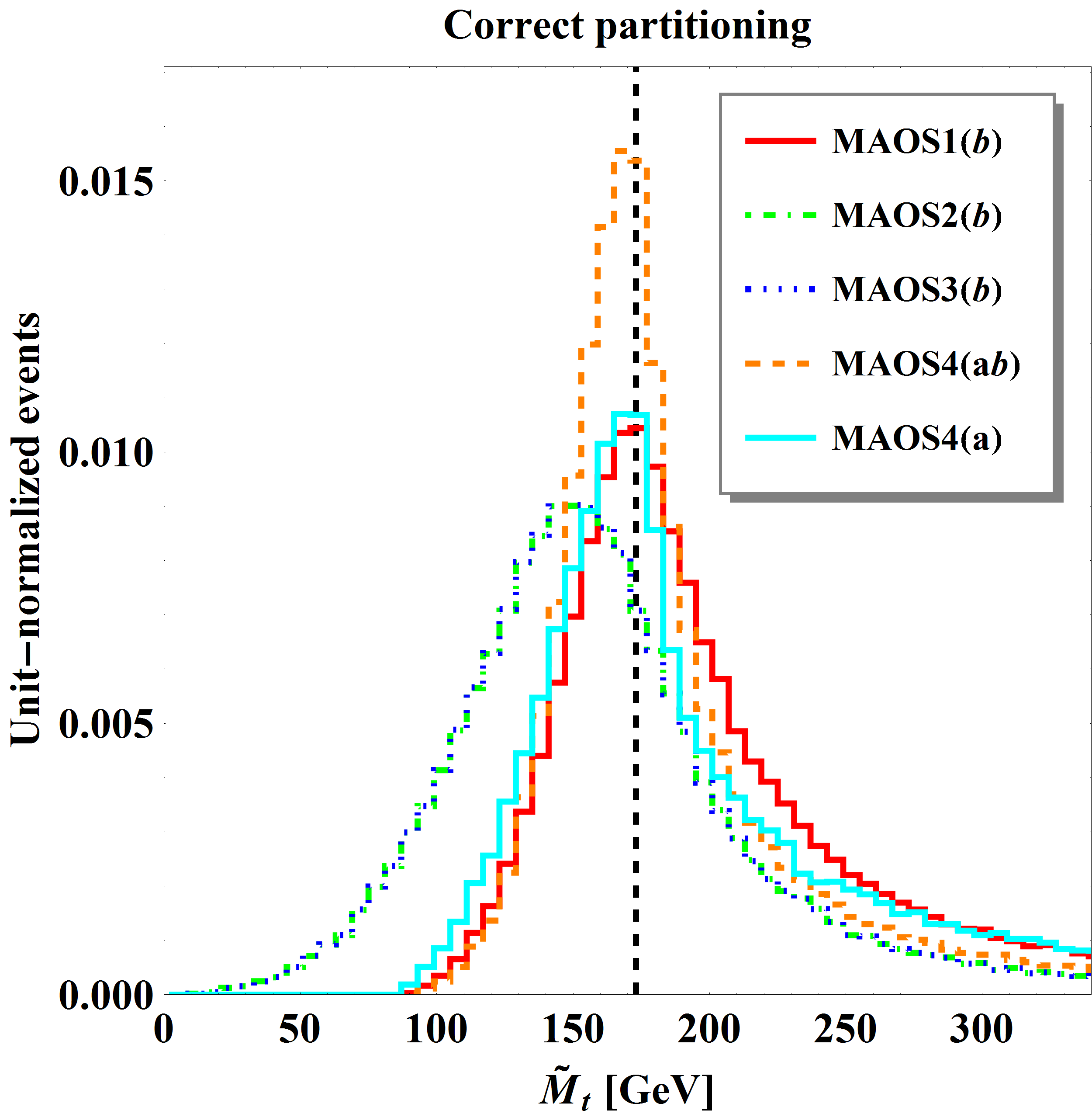
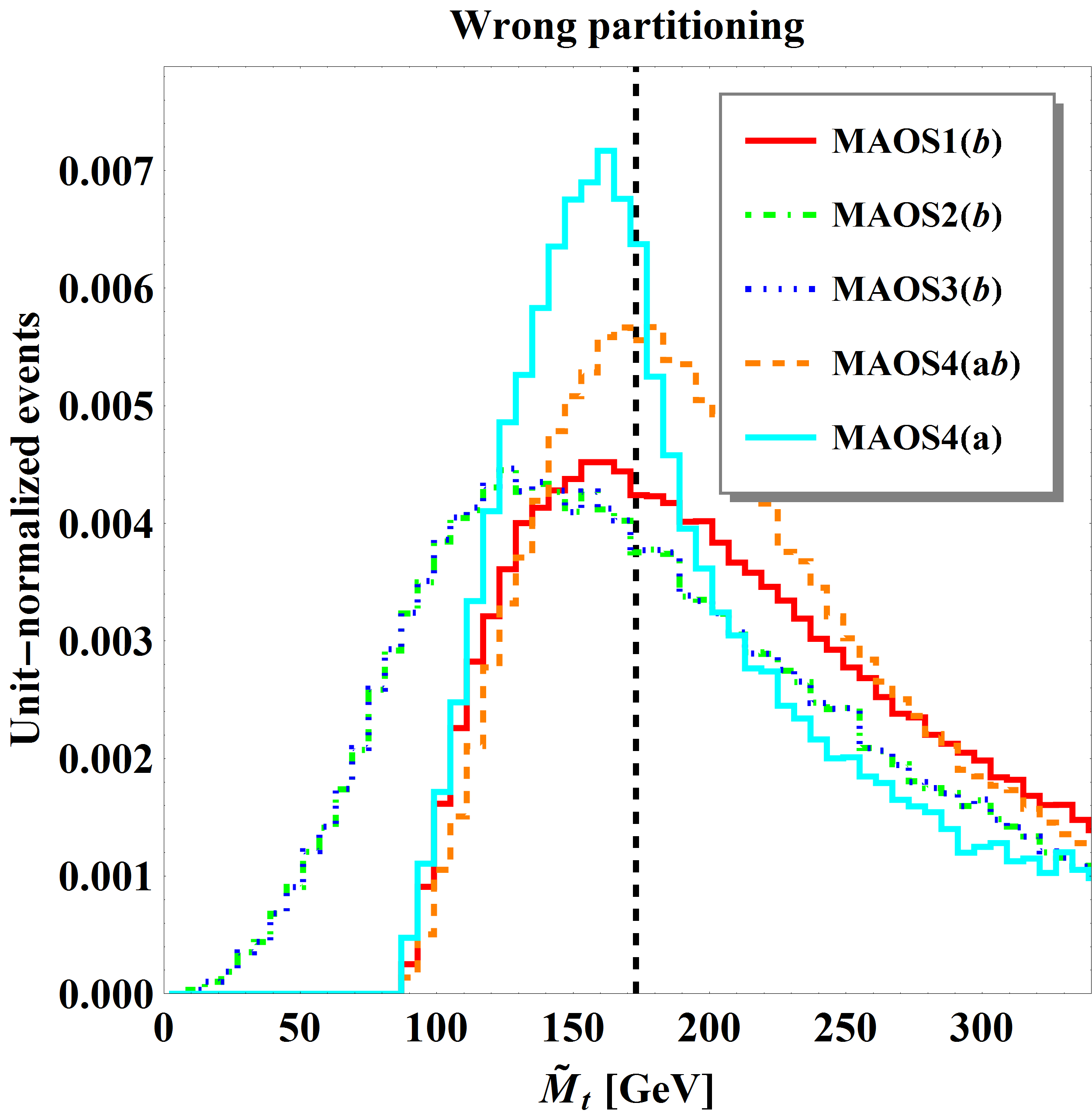
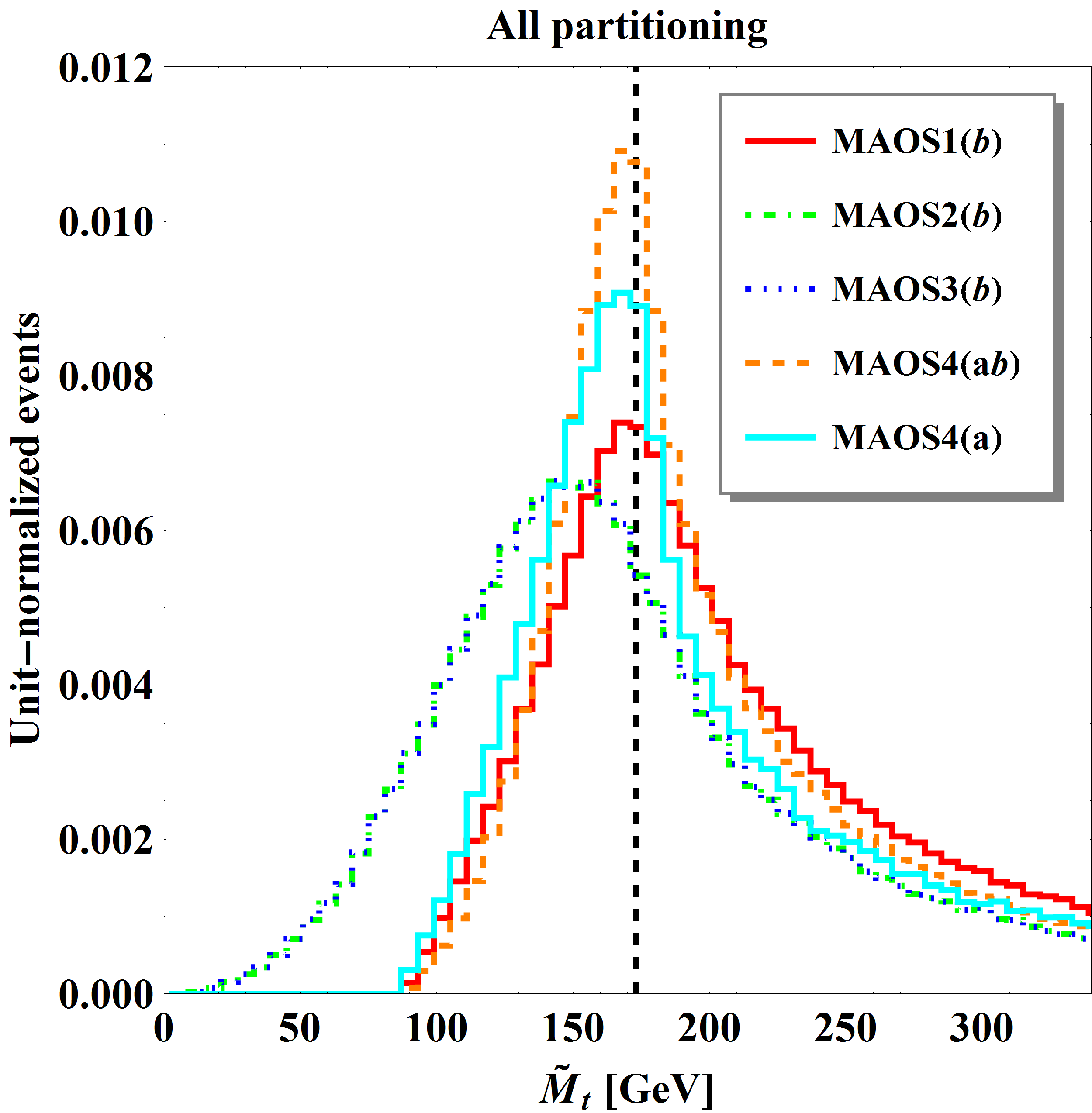
In all cases, we use the correct test mass when calculating $M_{T2}$: the true neutrino mass $m_{\nu}=0$ in subsystems (ab) and (b), and the true $W$-boson mass $m_{W}=80$ GeV for subsystem (a). In the case of MAOS2(b) and MAOS3(b), this is the only mass input needed to reconstruct $\tilde{M}_{t}$, see Table 1. Unfortunately, this theoretical advantage seems to be offset by the inferior performance of these two methods: even for the correct lepton-jet combination, the MAOS2(b) and MAOS3(b) distributions in the left panel in Fig. 2 peak below the true top mass $m_{t}$, so that a bump hunt will systematically underestimate the value of $m_{t}$. The remaining three MAOS methods illustrated in the figure, MAOS1(b), MAOS4(ab) and MAOS4(a), use an additional mass input, and are thus expected to perform better. This is confirmed by Fig. 2, which suggests that MAOS4(ab) slightly outperforms the other other two methods, MAOS4(a) and MAOS1(b), which are utilizing the smaller individual subsystems (a) and (b). There are two effects which contribute to this. First, for the correct lepton-jet combination (the left panel in Fig. 2) the distributions for all three methods, MAOS1(b), MAOS4(ab) and MAOS4(a), have their peaks very close to the true mass $m_{t}$, but the peak for MAOS4(ab) is more narrow than the other two. Second, for the wrong lepton-jet combination (the middle panel in Fig. 2), the MAOS4(ab) distribution is relatively broad, but happens to peak right around the top quark mass again, while the distributions for MAOS4(a) and MAOS1(b) peak at slightly lower values. If one does not attempt to resolve the combinatorics Rajaraman:2010hy ; Baringer:2011nh ; Choi:2011ys and instead does the simplest thing, namely, combine the two distributions from the left and middle panels of Fig. 2, one would obtain the combined distributions shown in the right panel of Fig. 2. We see that among the methods using two mass inputs, MAOS4(ab) appears to be the best, followed by MAOS4(a) and MAOS1(b). The remaining two procedures, MAOS2(b) and MAOS3(b), rely on a single mass input, and give identical answers, in accordance with our expectations for subsystem $(b)$.

Figure 3: Comparison of the performance of different MAOS schemes in reconstructing the $W$-boson mass in dilepton $t\bar{t}$ events. Distributions of the reconstructed $W$-boson mass $\tilde{M}_{W}$ are shown for the case of the correct lepton-jet pairing (left panel), the wrong lepton-jet pairing (middle panel) and both pairings (right panel). The $W$-boson is treated as a relative particle in the case of MAOS1(ab) (red solid line), MAOS2(ab) (green dot-dashed line) and MAOS3(ab) (blue dotted line), and as a parent particle in the case of MAOS4(b) (orange dashed line).

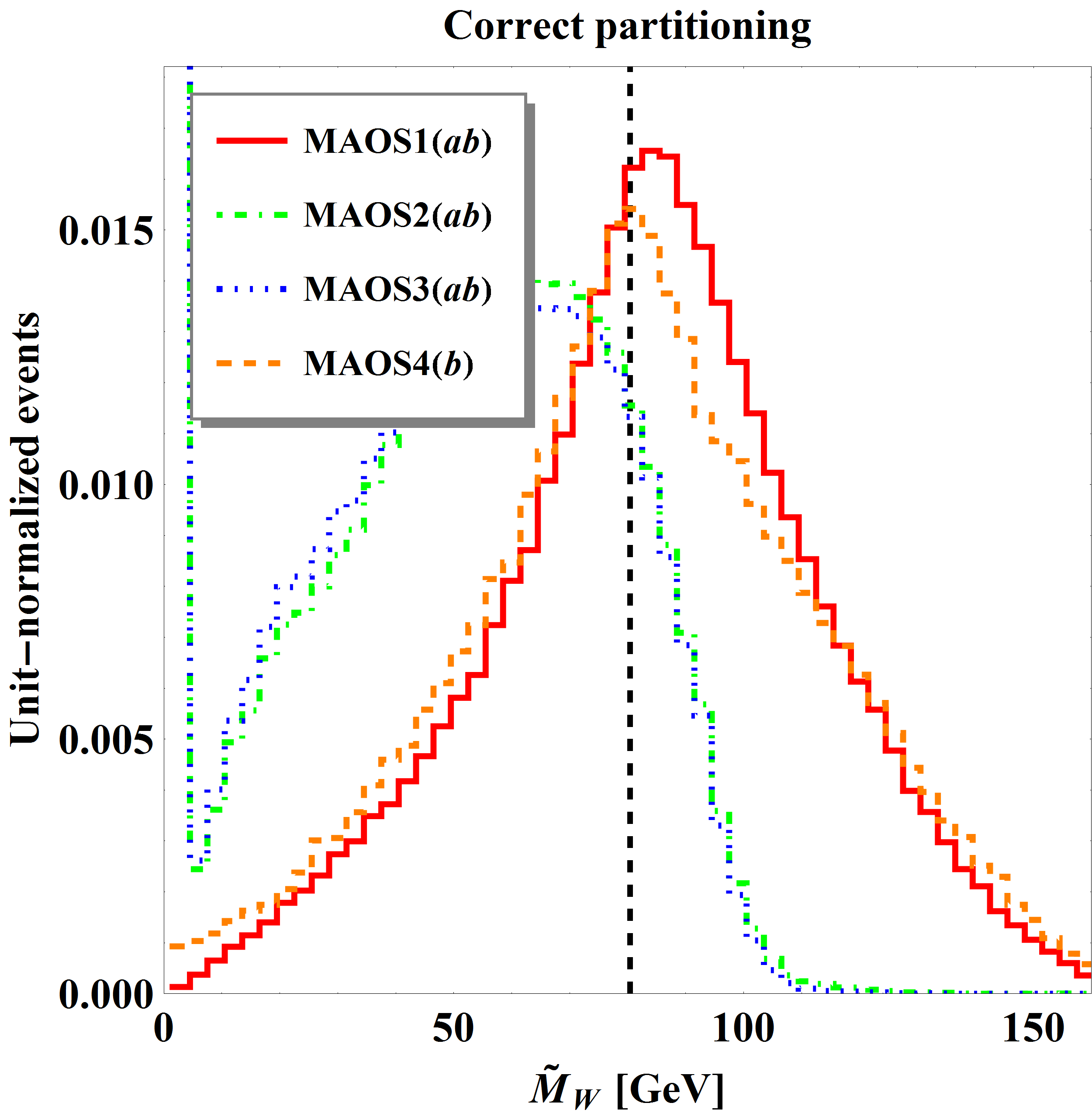
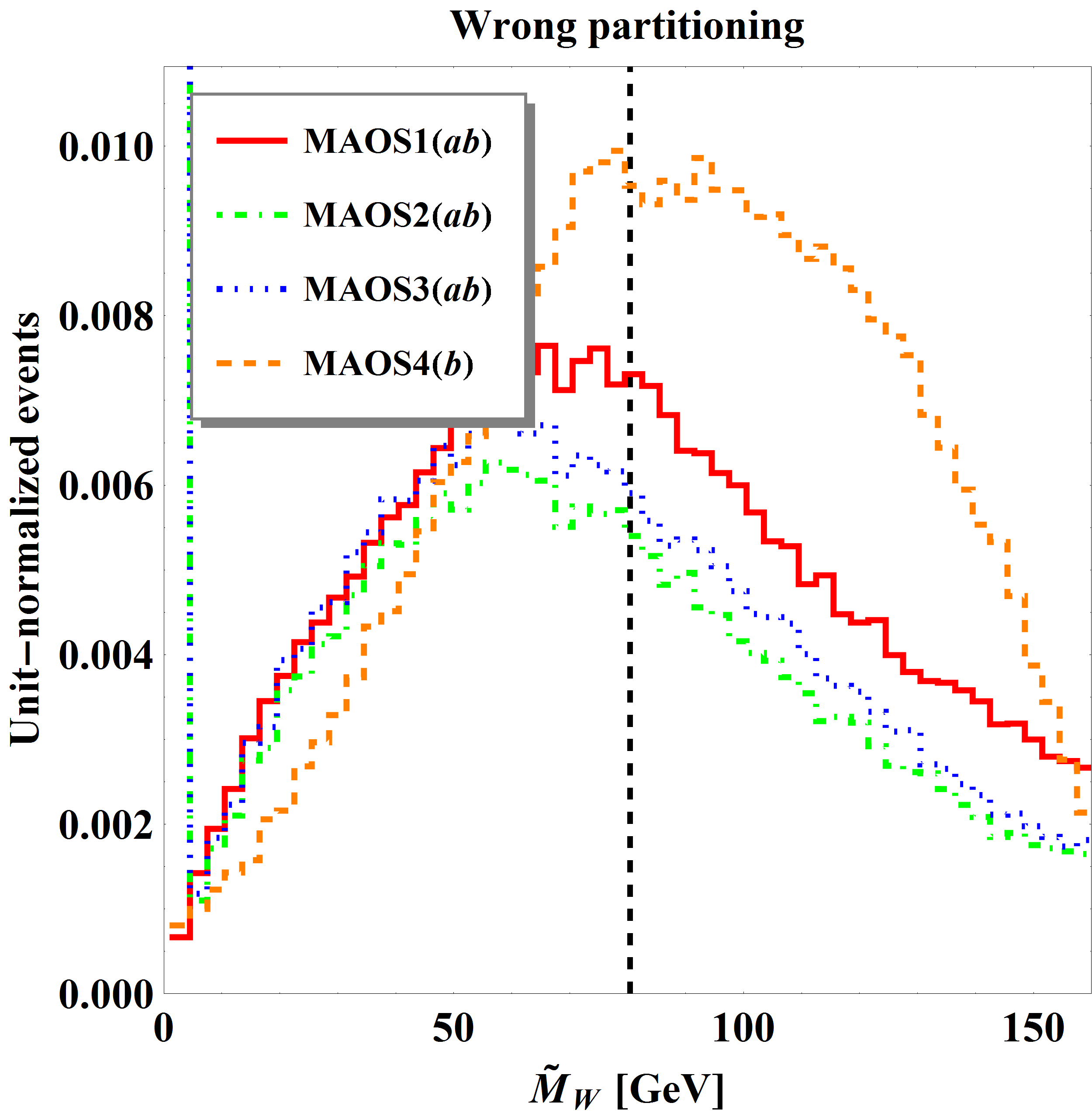
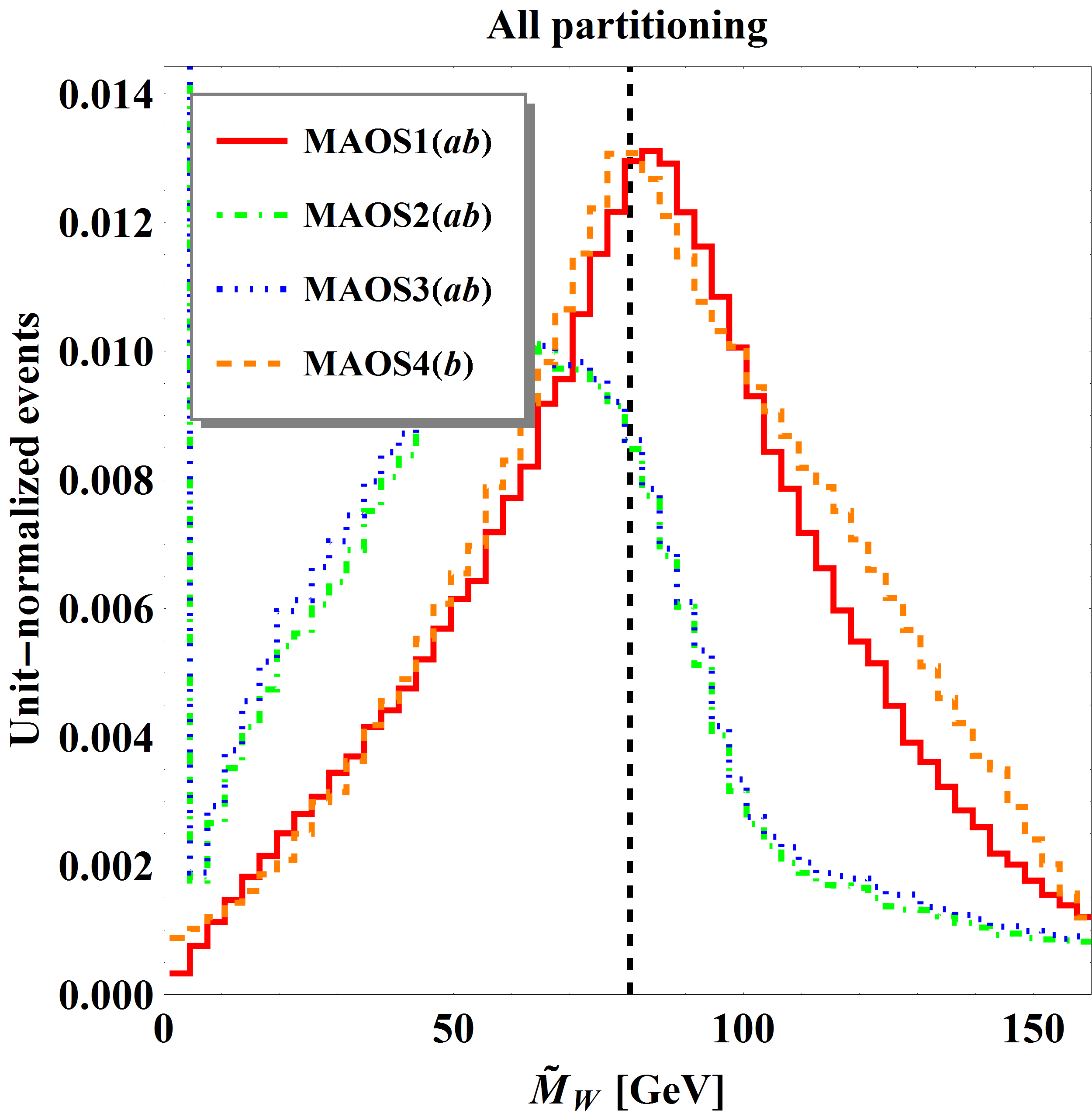
Fig. 3 shows the analogous results for the reconstruction of the mass $\tilde{M}_{W}$ of the $W$-boson, using MAOS1(ab) (red solid line), MAOS2(ab) (green dot-dashed line), MAOS3(ab) (blue dotted line), and MAOS4(b) (orange dashed line). In all cases we use the correct test mass as an input to the $M_{T2}$ calculation, and then the correct value of the additional mass input required for MAOS1(ab) and MAOS4(b). The left panel of Fig. 3 clearly demonstrates the benefit of the additional mass input, as MAOS1(ab) and MAOS4(b) greatly outperform MAOS2(ab) and MAOS3(ab). Since the corresponding wrong-combination distributions in the middle panel have similar shapes, this advantage is preserved in the combined distributions shown in the right panel. Upon closer inspection, MAOS4(b) (orange dashed line) appears slightly better than MAOS1(ab) (red solid line). However, in new physics applications of the MAOS methods, the knowledge of the additional mass input is not always guaranteed, and one would have to do with MAOS2(ab) or MAOS3(ab), which perform very similarly. Among the two, MAOS3(ab) has a slight theoretical advantage in the sense that its invisible momentum ansatz is always unique and well-defined.

Figure 4: Comparison of the performance of different MAOS schemes in reconstructing the neutrino mass-squared in dilepton $t\bar{t}$ events. Distributions of the reconstructed neutrino mass-squared $\tilde{M}^{2}_{\nu}$ are shown for the case of the correct lepton-jet pairing (left panel), the wrong lepton-jet pairing (middle panel) and both pairings (right panel). Here the neutrino is always treated as a relative particle in the case of MAOS1(a) (red solid line), MAOS2(a) (green dot-dashed line) and MAOS3(a) (blue dotted line).

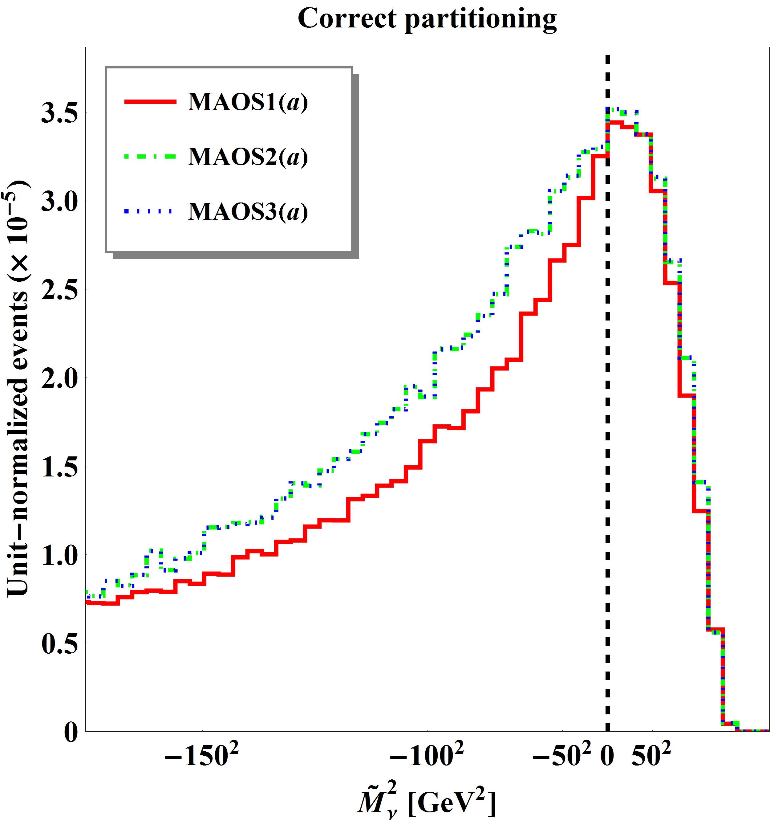
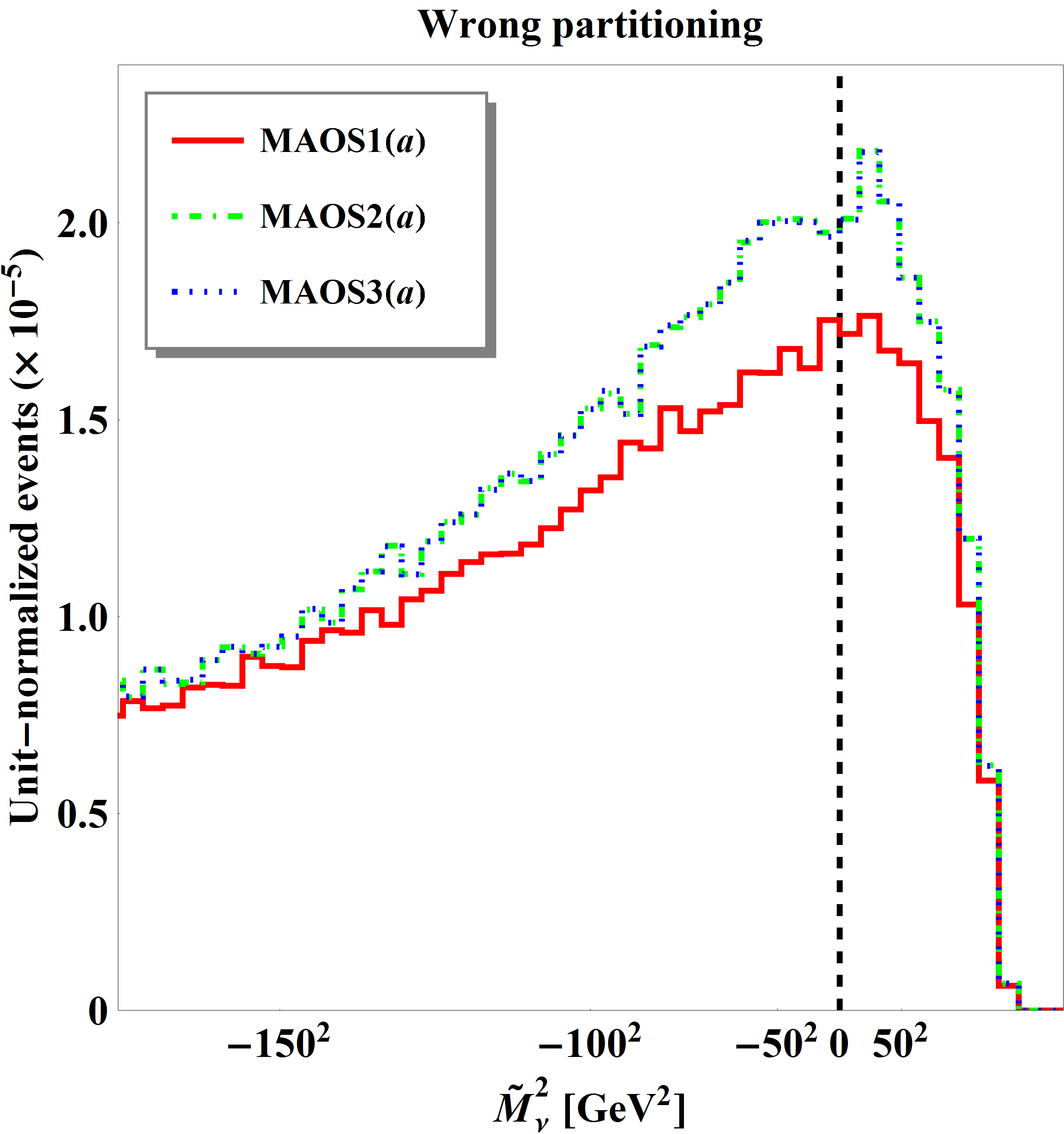
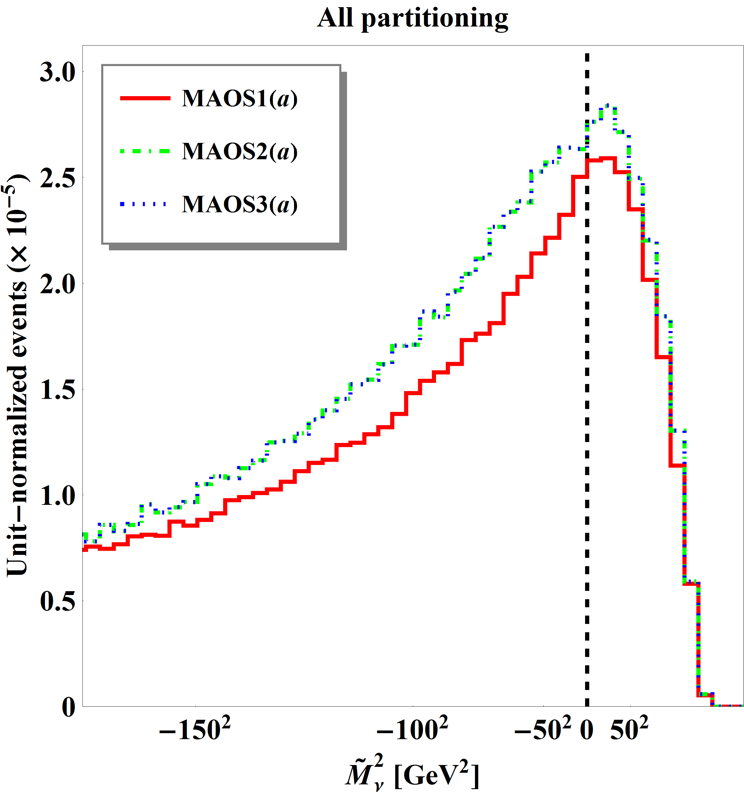
Our third and final mass reconstruction for the dilepton $t\bar{t}$ topology is shown in Fig. 4, where we plot in analogous fashion the reconstructed neutrino mass-squared $\tilde{M}^{2}_{\nu}$ when the neutrino is treated as a relative particle in subsystem (a): MAOS1(a) (red solid line), MAOS2(a) (green dot-dashed line) and MAOS3(a) (blue dotted line). This time the benefit of the additional mass input $m_{t}$ in the case of MAOS1(a) is not so clear — all three distributions have similar shapes (the distributions for MAOS2(a) and MAOS3(a) are in fact identical, since subsystem $(a)$ has only balanced events) and peak near the origin.

4.2 Comparison of the different $M_{2}$-based methods

We shall now use the dilepton $t\bar{t}$ example to test the accuracy of the invisible momentum reconstruction from the different $M_{2}$-based methods listed in Table 2. We shall not consider all 18 possibilities in Table 2, since some are closely related. For example, it is known that for any subsystem, the $M_{2XX}$ and $M_{2CX}$ variables are identical, and furthermore, equal to the value of the Cambridge transverse mass variable $M_{T2}$ Cho:2014naa :

$$M_{2XX}=M_{2CX}=M_{T2}.$$ (40)

In spite of this relation, the corresponding three ansatze for the invisible momenta are not necessarily the same. First of all, $M_{T2}$ is a transverse variable and it only fixes the transverse components $\vec{q}_{1T}$ and $\vec{q}_{2T}$, while $M_{2XX}$ and $M_{2CX}$ in addition provide values for the longitudinal components $q_{1z}$ and $q_{2z}$. In the case of balanced events, those predictions are unique and the same for $M_{2XX}$ and $M_{2CX}$, while for unbalanced events, there is a two-fold ambiguity for $q_{1z}$ and $q_{2z}$ in the case of $M_{2CX}$ and a flat direction in the case of $M_{2XX}$ Cho:2014naa . In what follows, we shall therefore prefer to consider the invisible momentum reconstruction from the $M_{2CX}$ variable instead of $M_{2XX}$.

Similar considerations apply in the case of the pair of variables $M_{2XC}$ and $M_{2CC}$, as well as for $M_{2XR}$ and $M_{2CR}$. In each case, the variables are equal for balanced events and only differ for unbalanced events, where this time the obtained invisible momentum configurations are unique. This is why we shall also not consider $M_{2XC}$ and $M_{2XR}$, and instead focus on $M_{2CC}$ and $M_{2CR}$, respectively.

Figure 5: The same as Fig. 2, but using the appropriate $M_{2}$ variables for fixing the invisible momenta. Distributions of $\tilde{M}_{t}$ are shown for the case of $M_{2CR}(ab)$ (red solid line), $M_{2CX}(b)$ (green dot-dashed line), $M_{2CC}(b)$ (blue dotted line), and $M_{2CR}(a)$ (orange dashed line).

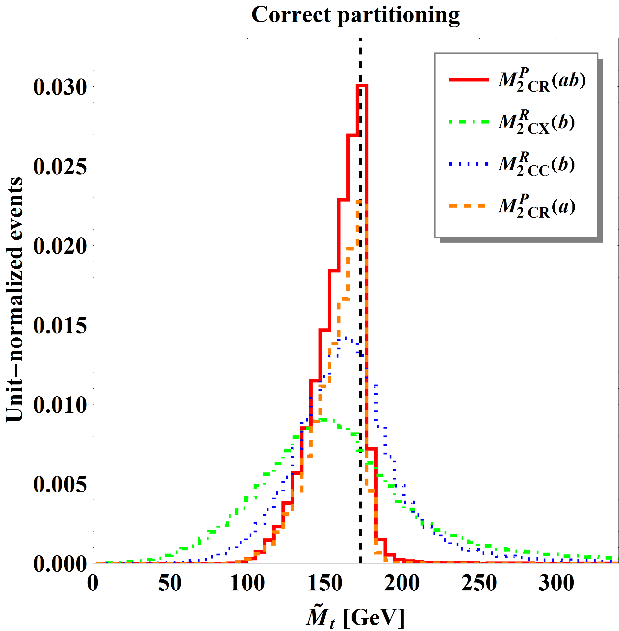
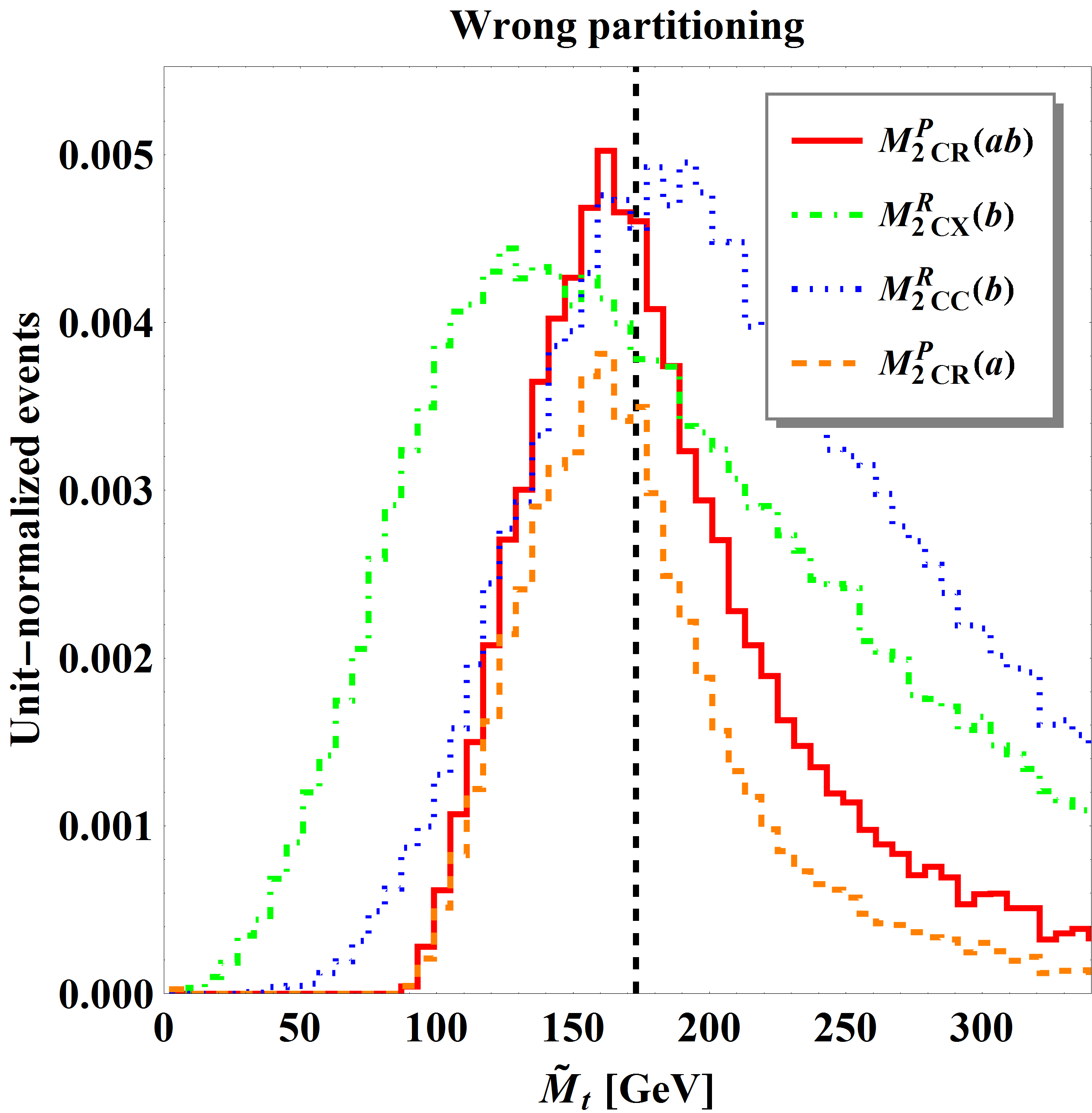
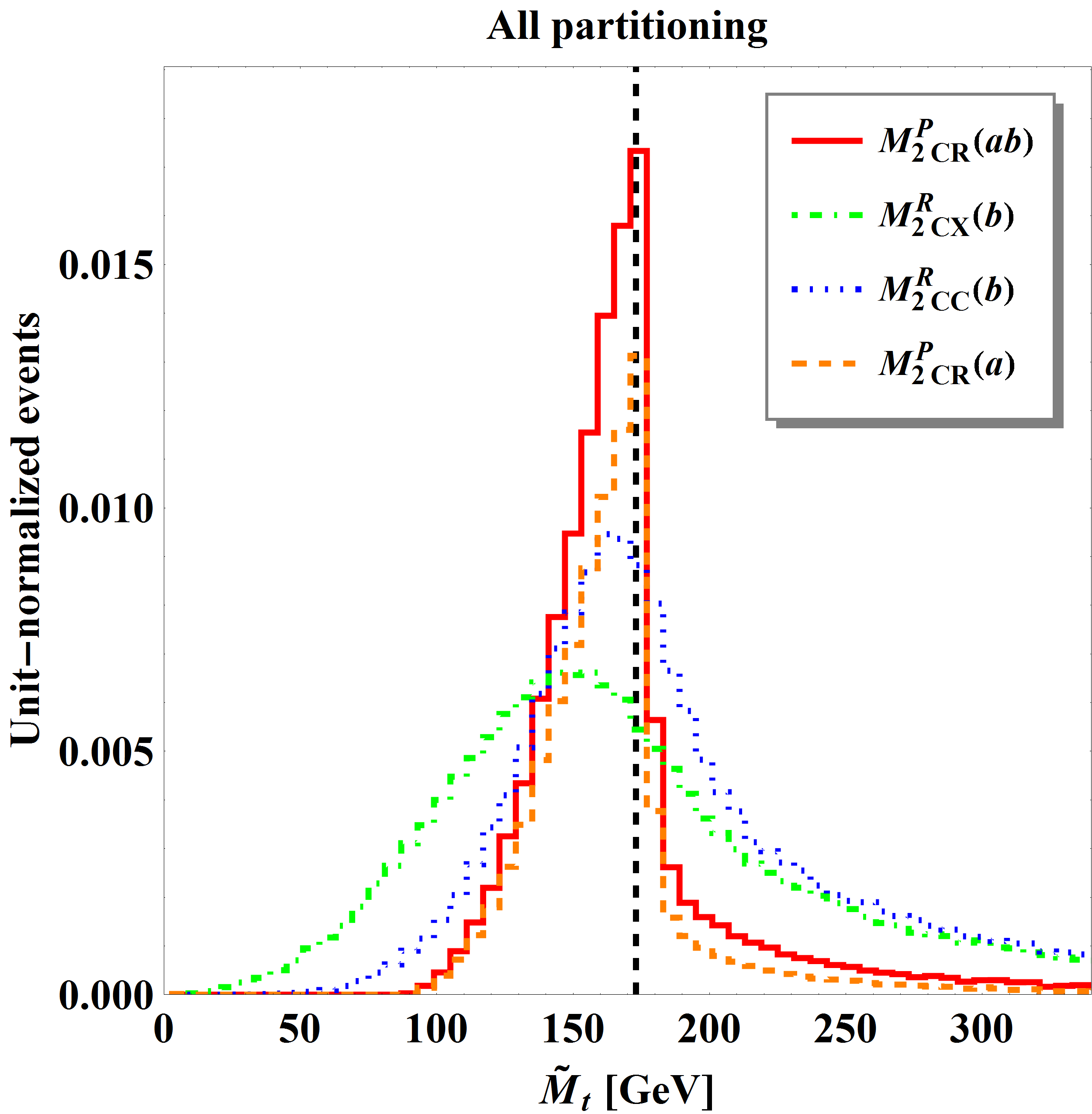
Fig. 5 shows distributions of the reconstructed top quark mass $\tilde{M}_{t}$ with the four relevant $M_{2}$ methods from Table 2: $M_{2CR}(ab)$ (red solid line), $M_{2CX}(b)$ (green dot-dashed line), $M_{2CC}(b)$ (blue dotted line), and $M_{2CR}(a)$ (orange dashed line). In analogy to Fig. 2, we show separately the distributions obtained for the correct lepton-jet pairing (left panel), the wrong lepton-jet pairing (middle panel), and both pairings (right panel). Note that some distributions have fewer events, since the constraints cannot be simultaneously satisfied. This is most notable for the case of $M_{2CR}(a)$, and is typically due to events in which an intermediate resonance (a top quark or a $W$-boson) is rather off-shell (we expect this effect to be further amplified once we account for the finite detector resolution). Also note that in subsystems $(ab)$ and $(a)$ the top quark is a parent particle, while in subsystem $(b)$ it is a relative particle. This distinction is indicated in the legend of Fig. 5 with a superscript $P$ or $R$, respectively.

Fig. 5 confirms that the more constrained variables generally provide better guesses for the invisible momenta, as measured by the location and width of the reconstructed mass peak in $\tilde{M}_{t}$. The most constrained version of the $M_{2}$ variable is $M_{2CR}$, which has one parent constraint and two relative constraints, leaving a single momentum degree of freedom to be minimized over. In Fig. 5, both $M_{2CR}(ab)$ and $M_{2CR}(a)$ seem to work very well — for the correct lepton-jet pairing, the reconstructed top mass peak is very well defined and located at the correct position (marked with the vertical dashed line). However, the disadvantage of $M_{2CR}(ab)$ and $M_{2CR}(a)$ is that one uses both the $W$-boson mass and the neutrino mass as inputs to the calculation, which restricts their applicability to BSM scenarios. Under those circumstances, the single-input variables $M_{2CX}(b)$ and $M_{2CC}(b)$ will be more useful for momentum reconstruction — in Fig. 5 the corresponding $\tilde{M}_{t}$ distributions are shown with the green dot-dashed and the blue dotted line, respectively. We see that even with the lack of knowledge of the precise value of the $W$-boson mass, the $M_{2CC}(b)$ variable still provides a good momentum ansatz, as judged by the location of the peak of its $\tilde{M}_{t}$ distribution.

Figure 6: The same as Fig. 3, but using the appropriate $M_{2}$ variables for fixing the invisible momenta. Distributions of $\tilde{M}_{W}$ are shown for the case of $M_{2CX}(ab)$ (green dot-dashed line), $M_{2CC}(ab)$ (blue dotted line), and $M_{2CR}(b)$ (red solid line).

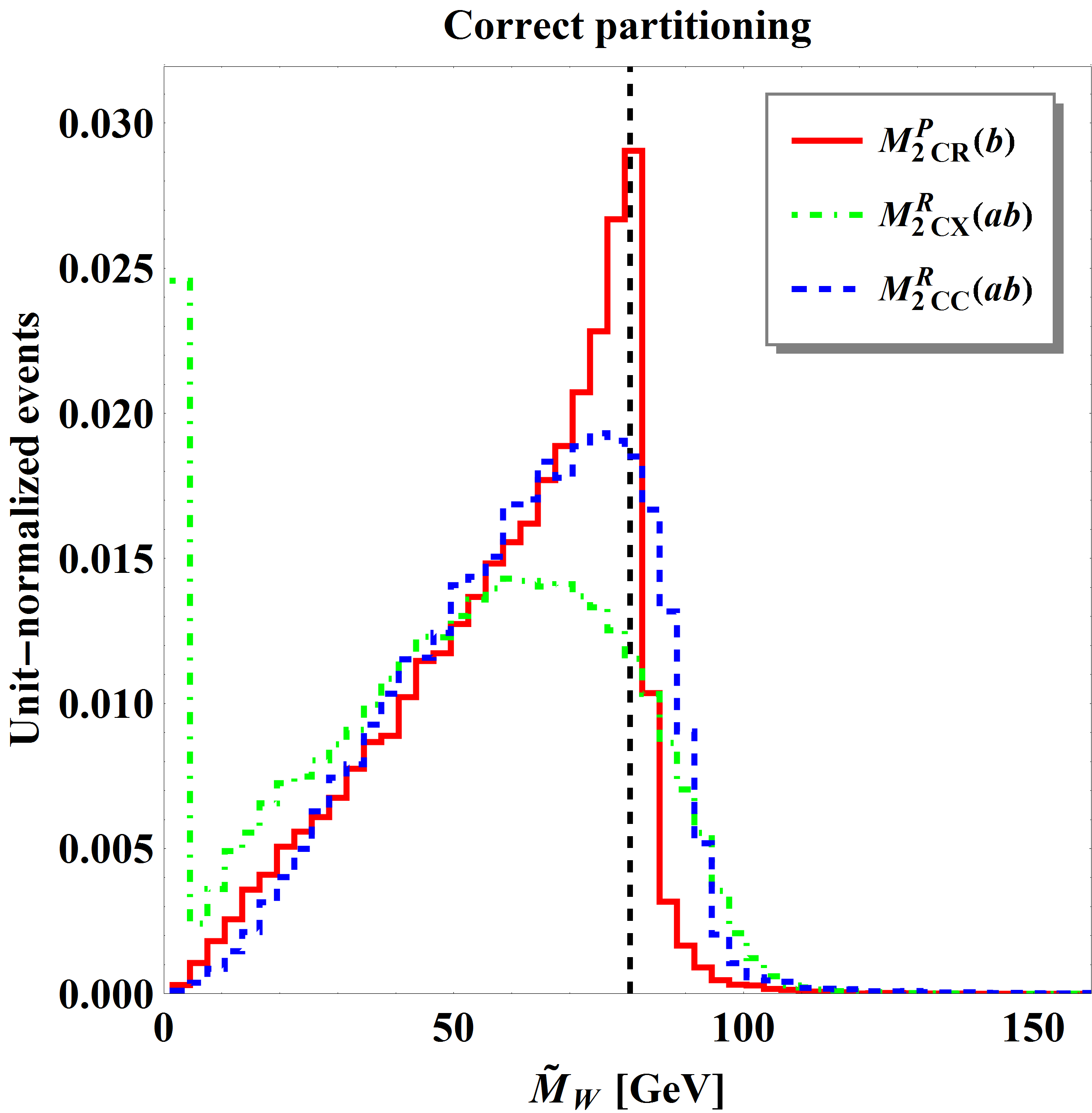
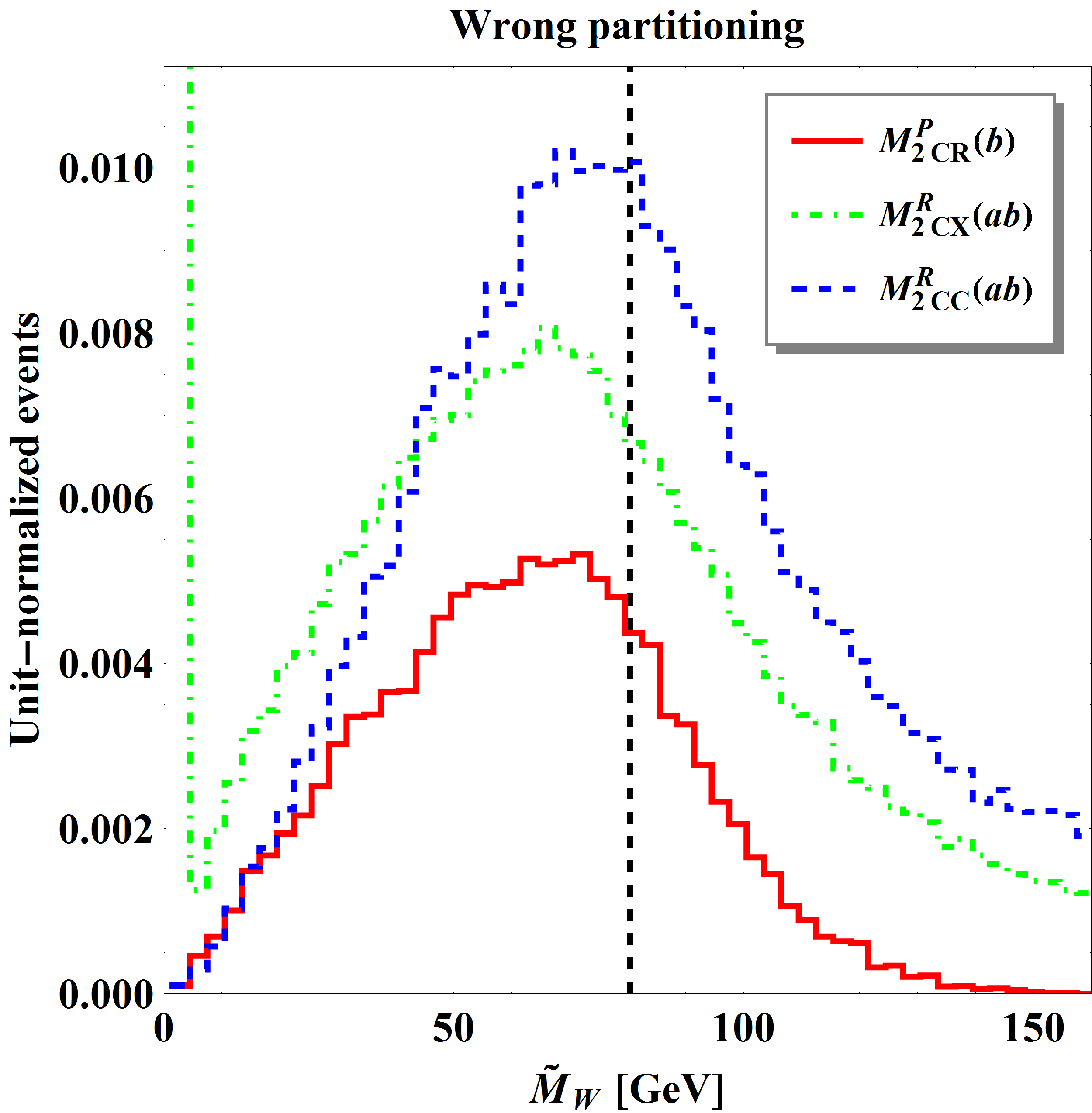
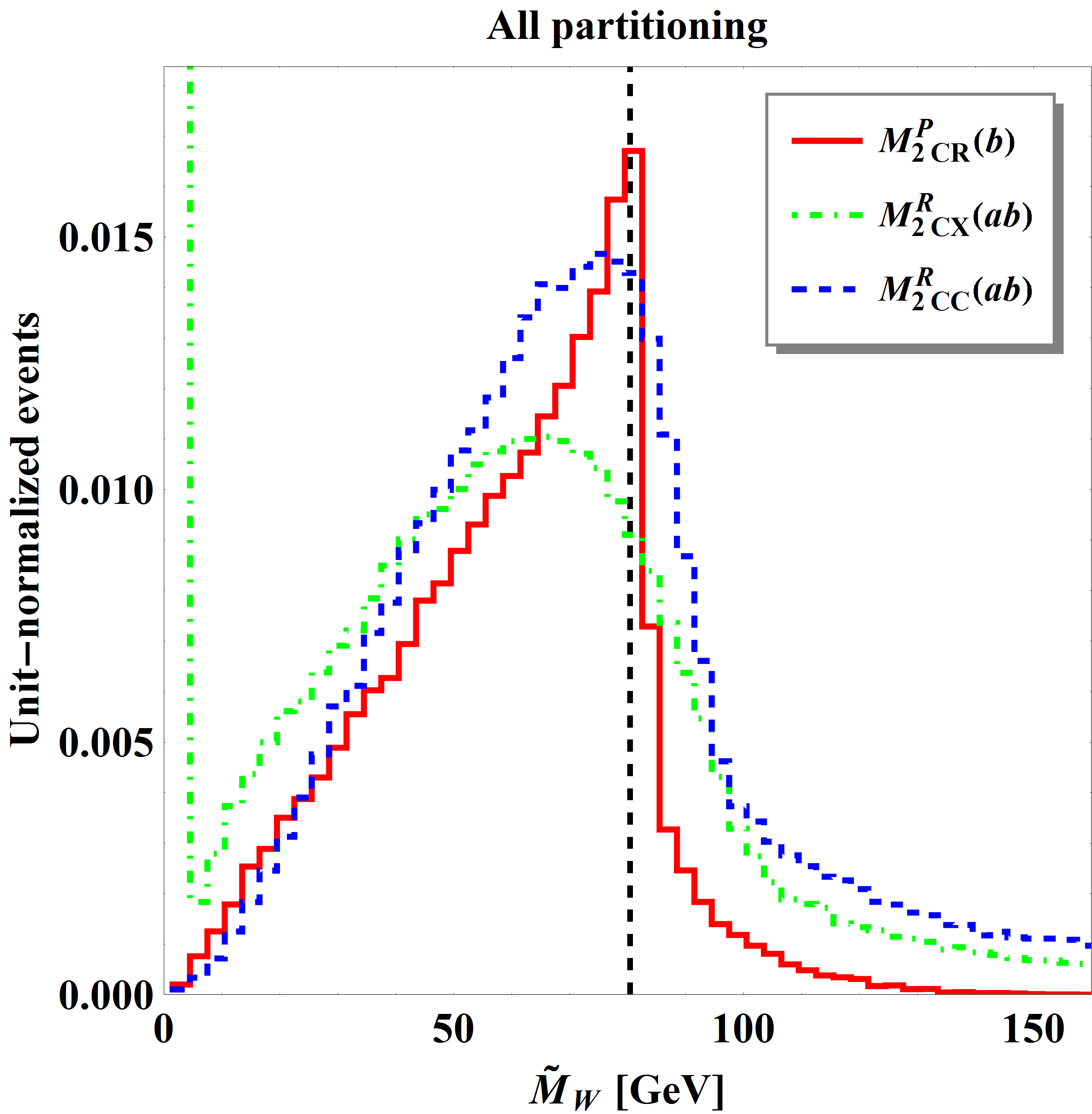
In Figs. 6 and 7 we similarly show distributions of the reconstructed $W$-boson mass $\tilde{M}_{W}$ and the reconstructed neutrino mass squared $\tilde{M}^{2}_{\nu}$, respectively. (These two figures are the analogues of Figs. 3 and 4 for the MAOS case.) The $\tilde{M}_{W}$ distributions in Fig. 6 use invisible momentum reconstruction from $M_{2CX}(ab)$ (green dot-dashed line), $M_{2CC}(ab)$ (blue dotted line), and $M_{2CR}(b)$ (red solid line), while the $\tilde{M}^{2}_{\nu}$ distributions in Fig. 7 use the invisible momenta obtained by $M_{2CX}(a)$ (red solid line) and $M_{2CC}(a)$ (blue dashed line). We again observe that the maximally constrained variable, $M_{2CR}(b)$, which uses as inputs the neutrino and top quark masses, is able to provide us with a very good ansatz for the invisible momenta, and the $\tilde{M}_{W}$ distribution in Fig. 6 exhibits a very narrow peak at the proper location (80 GeV). The remaining four distributions in Figs. 6 and 7 are derived from single-input variables, where we again observe that $M_{2CC}$ performs slightly better than $M_{2CX}$.

Figure 7: The same as Fig. 4, but using the appropriate $M_{2}$ variables for fixing the invisible momenta. Distributions of $\tilde{M}^{2}_{\nu}$ are shown for the case of $M_{2CX}(a)$ (red solid line) and $M_{2CC}(a)$ (blue dashed line).

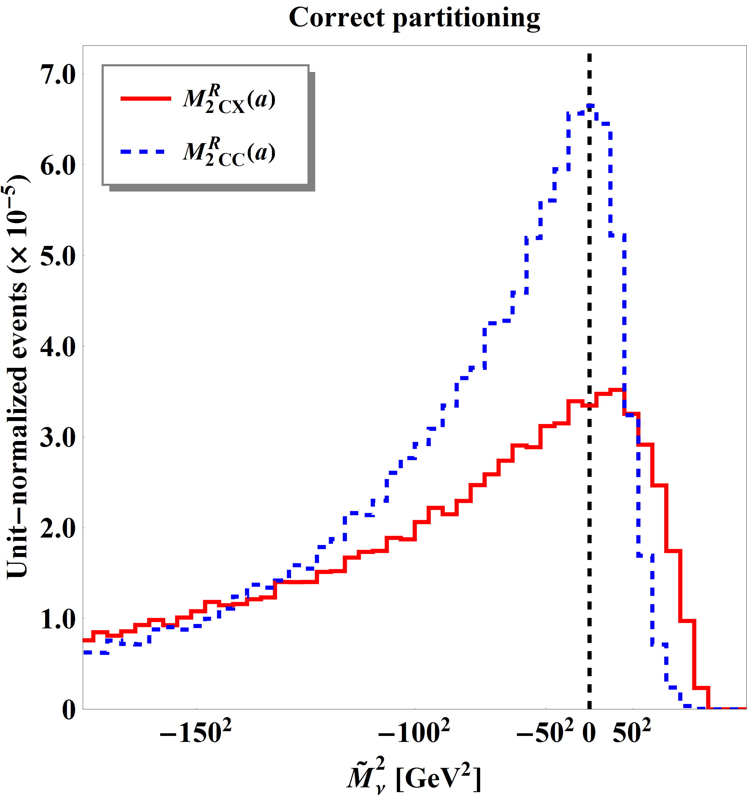
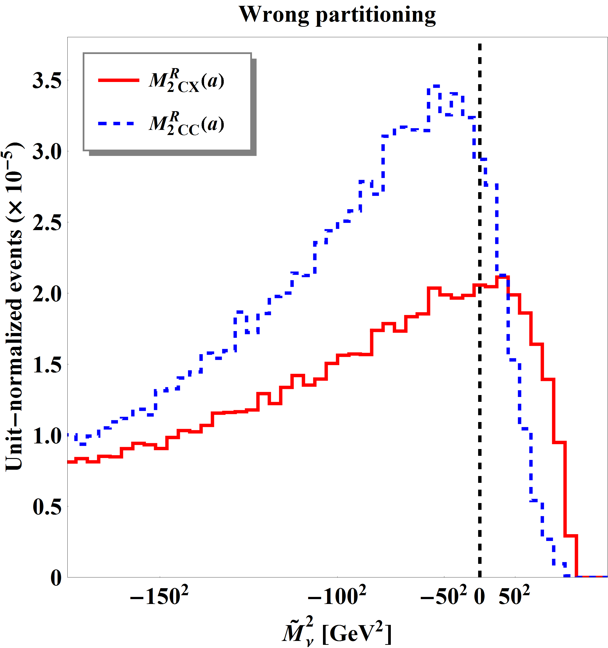
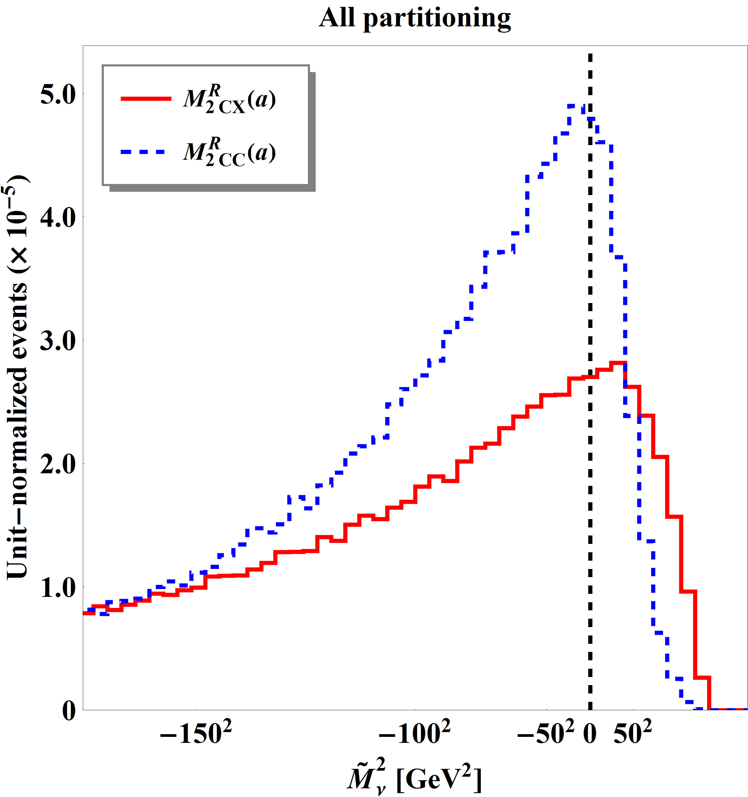
In the above discussion of Figs. 5 and 6 we have been focusing on measuring the top quark mass and the $W$-boson mass from the peaks of the respective $\tilde{M}_{t}$ and $\tilde{M}_{W}$ distributions. However, one should keep in mind that whenever we reconstruct a parent mass, we always have the option of measuring it from a kinematic endpoint as well. This is clearly evident in the left panel of Fig. 5 for the case of $M_{2CR}(ab)$ and $M_{2CR}(a)$, and in the left panel of Fig. 6 for the case of $M_{2CR}(b)$. Even with the pollution from the wrong combinatorics in the middle panels of Figs. 5 and 6, the endpoint structures are still preserved in the corresponding combined distributions shown in the right panels.

4.3 Comparison of $M_{T2}$-assisted and $M_{2}$-assisted reconstruction schemes

Having discussed the different versions of the more traditional MAOS method in Sec. 4.1 and the different options for $M_{2}$-assisted invisible momentum reconstruction in Sec. 4.2, we are now ready to contrast the two methods to each other. For this purpose, we reassemble the results from the previous two subsections in Figs. 8-10, so that only methods using the same number of theoretical mass inputs are compared on each plot: the distributions shown on the left panels of these figures require two mass inputs, while the distributions in the right panels need only one. Since we already showed the effects of combinatorics in the previous two subsections (compare the left and middle panels of Figs. 2-7), here for simplicity we plot only the combined distributions, which include both the correct and the wrong lepton-jet assignment. Naturally, the use of the extra mass input should allow for a better measurement, thus one should expect the distributions in the left panels of Figs. 8-10 to be more sharply peaked than those in the corresponding right panels.

Figure 8: Comparison of the MAOS and $M_{2}$-assisted methods for top mass reconstruction from Figs. 2 and 5. The left panel shows distributions of the reconstructed top mass $\tilde{M}_{t}$ with methods which use two mass inputs (the $W$-boson mass and the neutrino mass): the three MAOS methods from Fig. 2, MAOS4(ab) (blue solid line), MAOS1(b) (green dot-dashed line), and MAOS4(a) (cyan dotted line), and the two $M_{2}$-based methods from Fig. 5, $M_{2CR}(ab)$ (red solid line) and $M_{2CR}(a)$ (orange dashed line). The right panel shows distributions of the reconstructed top mass $\tilde{M}_{t}$ with methods which use a single mass input (the neutrino mass): MAOS2(b) (blue dotted line) and MAOS3(b) (green dot-dashed line) from Fig. 2 and $M_{2CX}(b)$ (orange dashed line) and $M_{2CC}(b)$ (red solid line) from Fig. 5.

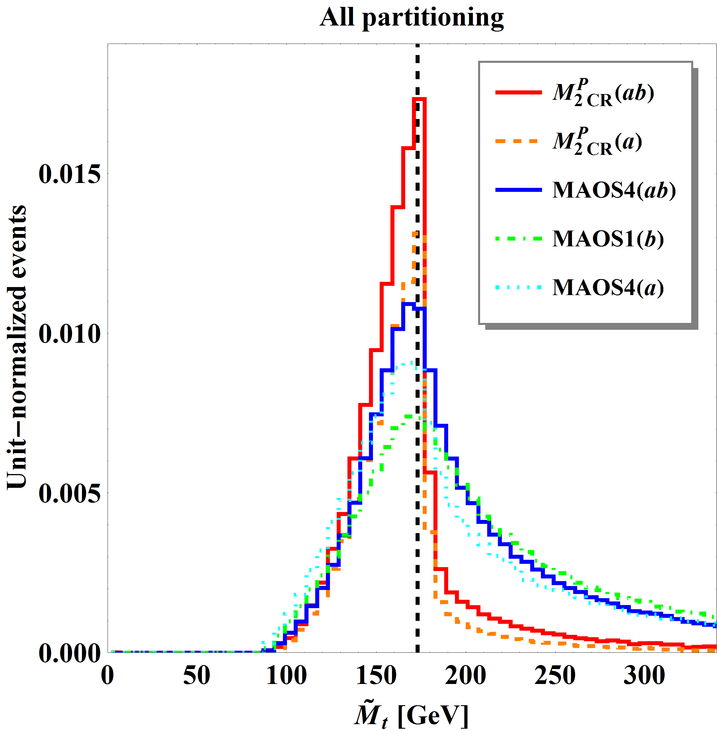
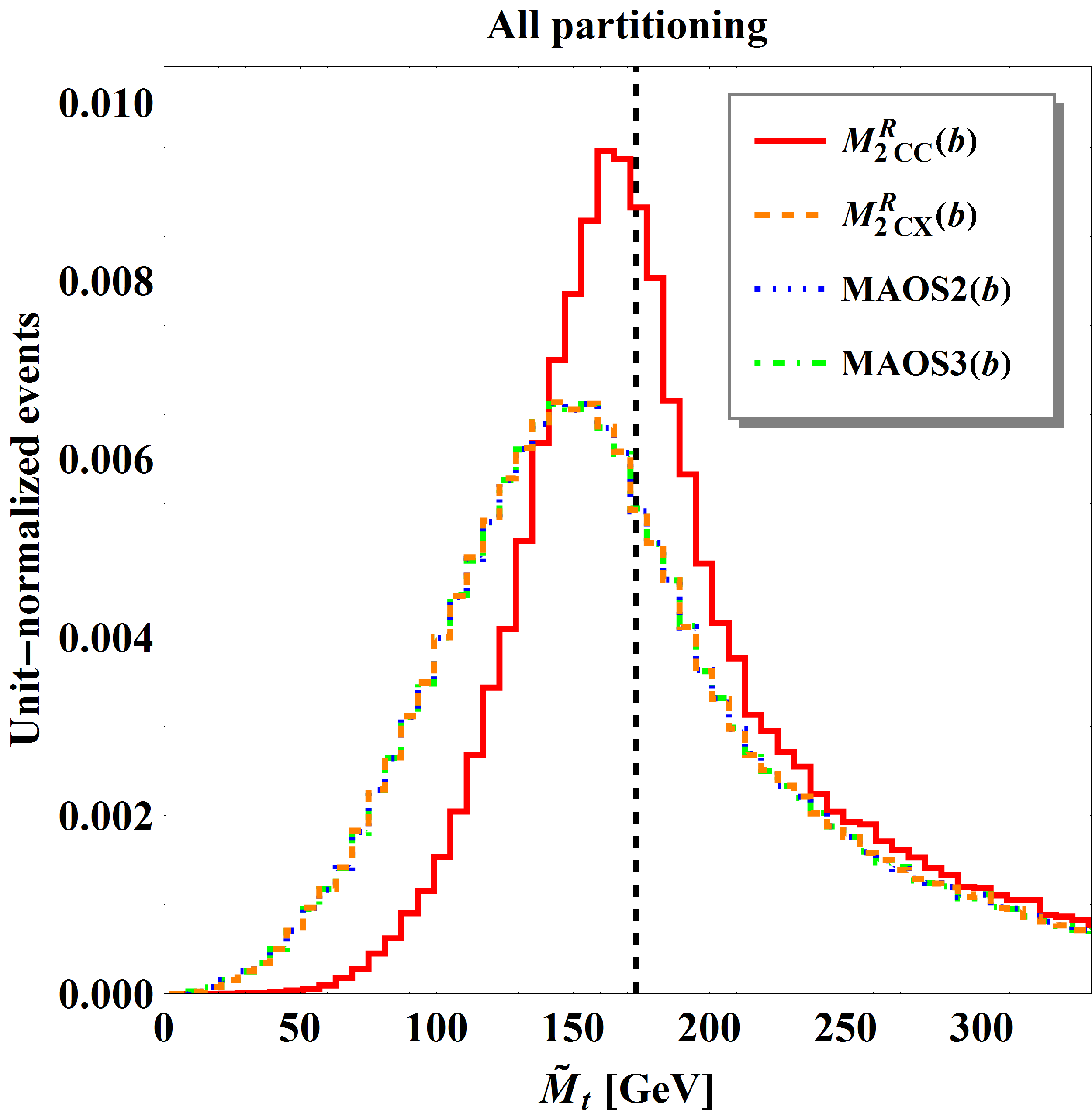
Fig. 8 summarizes our previous results from Figs. 2 and 5 for the reconstruction of the top mass $\tilde{M}_{t}$. The distributions shown in the left panel require prior knowledge of both the $W$-boson mass $m_{W}$ and the neutrino mass $m_{\nu}$, while for the distributions shown in the right panel one only needs to know $m_{\nu}$. The left panel of Fig. 8 demonstrates that the two $M_{2}$ methods, $M_{2CR}(ab)$ (the red solid line) and $M_{2CR}(a)$ (the orange dashed line) clearly outperform their MAOS counterparts, MAOS4(ab) (blue solid line), MAOS1(b) (green dot-dashed line) and MAOS4(a) (cyan dotted line) — the peaks reconstructed by means of $M_{2}$ are significantly more narrow, which should lead to a more precise mass measurement. Regardless of this width difference, in all five cases the peak of the distribution is correctly centered on the true top mass used in the simulations (indicated by the vertical dashed line). The right panel of Fig. 8 leads to a very similar conclusion for the set of methods which rely on a single mass parameter input — here the method of $M_{2CC}(b)$ (red solid line) is clearly the best, while the other three, MAOS2(b) (blue dotted line), MAOS3(b) (green dot-dashed line), and $M_{2CX}(b)$ (orange dashed line), are in a perfect tie, which is not a numerical coincidence, but rather expected theoretically. First, the procedures of MAOS2 and MAOS3 differ only for unbalanced events, of which there are none in subsystem $(b)$. Furthermore, it is known that the variables $M_{T2}$ and $M_{2CX}$ are identical in any subsystem Cho:2014naa , see eq. (40). Therefore they would lead to the same invisible momentum reconstruction, which is indeed confirmed by the right panel in Fig. 8.

Figure 9: The same as Fig. 8, but for the reconstructed mass $\tilde{M}_{W}$ of the $W$-boson. The left panel shows distributions of the reconstructed $W$-boson mass $\tilde{M}_{W}$ with methods which use two mass inputs (the top mass and the neutrino mass): MAOS1(ab) (green dot-dashed line) and MAOS4(b) (blue dotted line) from Fig. 3 and $M_{2CR}(b)$ (red solid line) from Fig. 6. The right panel shows distributions of the reconstructed $W$-boson mass $\tilde{M}_{W}$ with methods which use a single mass input (the neutrino mass): MAOS2(ab) (blue dotted line) and MAOS3(ab) (green dot-dashed line) from Fig. 3 and $M_{2CX}(ab)$ (orange dashed line) and $M_{2CC}(ab)$ (red solid line) from Fig. 6.

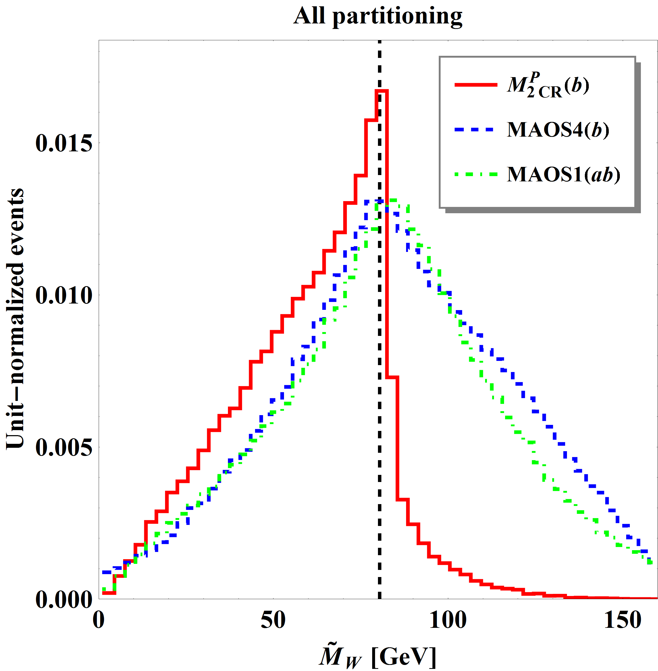
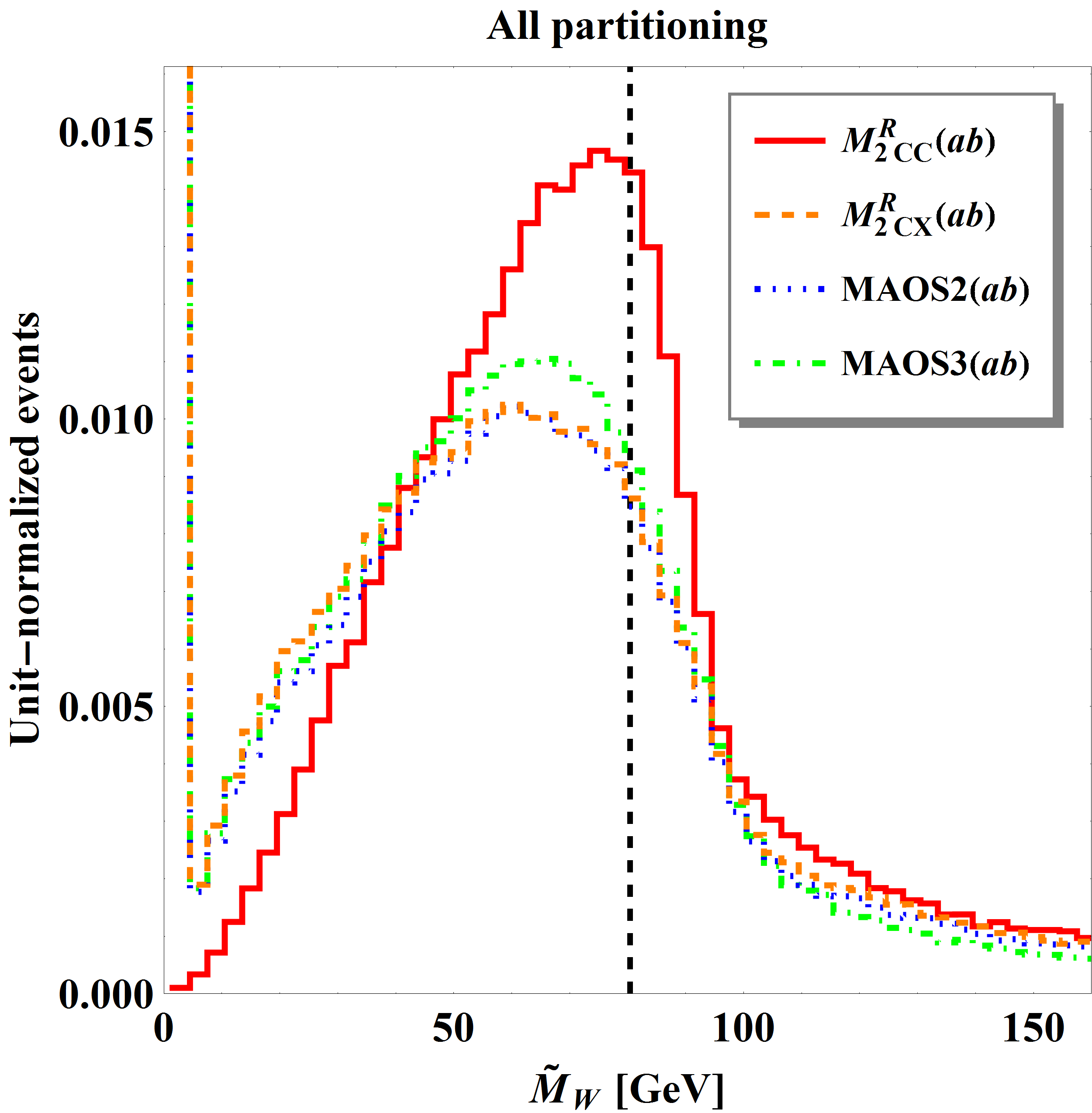
Fig. 9 reassembles our previous results from Figs. 3 and 6 for the reconstructed $W$-boson mass $\tilde{M}_{W}$. The left panel shows the distributions which need two mass inputs, the top mass $m_{t}$ and the neutrino mass $m_{\nu}$. All three distributions peak at the correct value of the $W$ mass indicated with the vertical dashed line. However, the distribution obtained with $M_{2CR}(b)$ (the red solid line) is slightly more narrow than the other two, corresponding to MAOS1(ab) (the green dot-dashed line) and MAOS4(b) (the blue dotted line). The right panel in Fig. 9 collects the distributions from Figs. 3 and 6 which require only the neutrino mass as an input. Here we notice that MAOS2(ab) (the blue dotted line) and MAOS3(ab) (the green dot-dashed line) give slightly different results, due to the presence of unbalanced events in subsystem $(ab)$. Once again, the theorem from Cho:2014naa ensures that the distributions for MAOS2(ab) (the blue dotted line) and $M_{2CX}(ab)$ (the orange dashed line) are the same. Just like we saw in the right panel of Fig. 8, the distribution obtained from the $M_{2CC}$-type variable, in this case $M_{2CC}(ab)$ (the red solid line), has the best properties: its peak is relatively narrow and appears closest to the true $W$-boson mass.

Figure 10: The same as Fig. 8, but for the reconstructed mass-squared $\tilde{M}^{2}_{\nu}$ of the neutrino. The left panel shows the distribution obtained with MAOS1(a) from Fig. 4, which uses two mass inputs: the mass of the top quark and the mass of the $W$-boson. The right panel shows distributions of the reconstructed neutrino mass squared $\tilde{M}^{2}_{\nu}$ with methods which use a single mass input (the $W$-boson mass): MAOS2(a) (blue dotted line), and MAOS3(a) (green dot-dashed line) from Fig. 4 and $M_{2CX}(a)$ (orange dashed line) and $M_{2CC}(a)$ (red solid line) from Fig. 7.

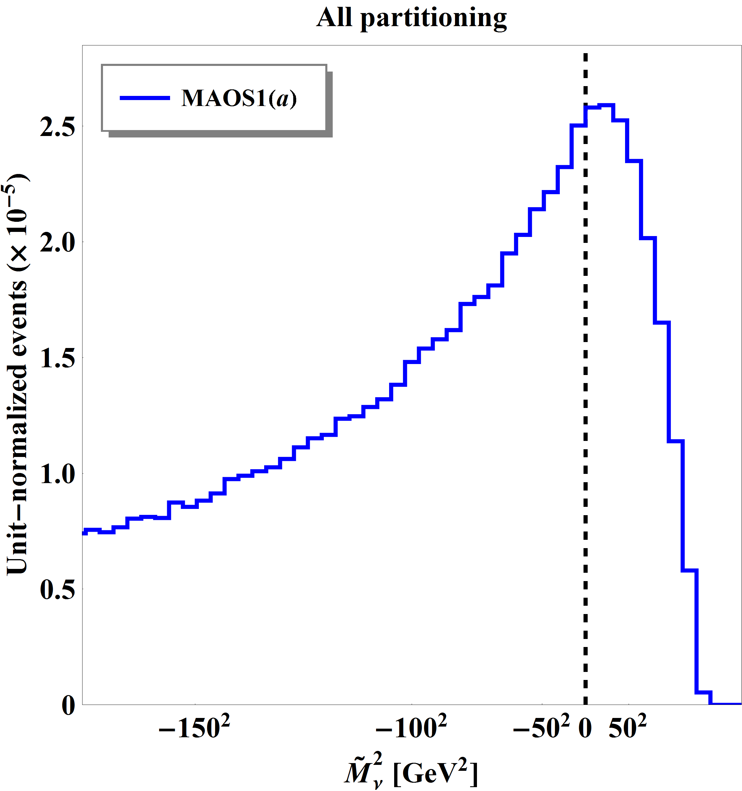
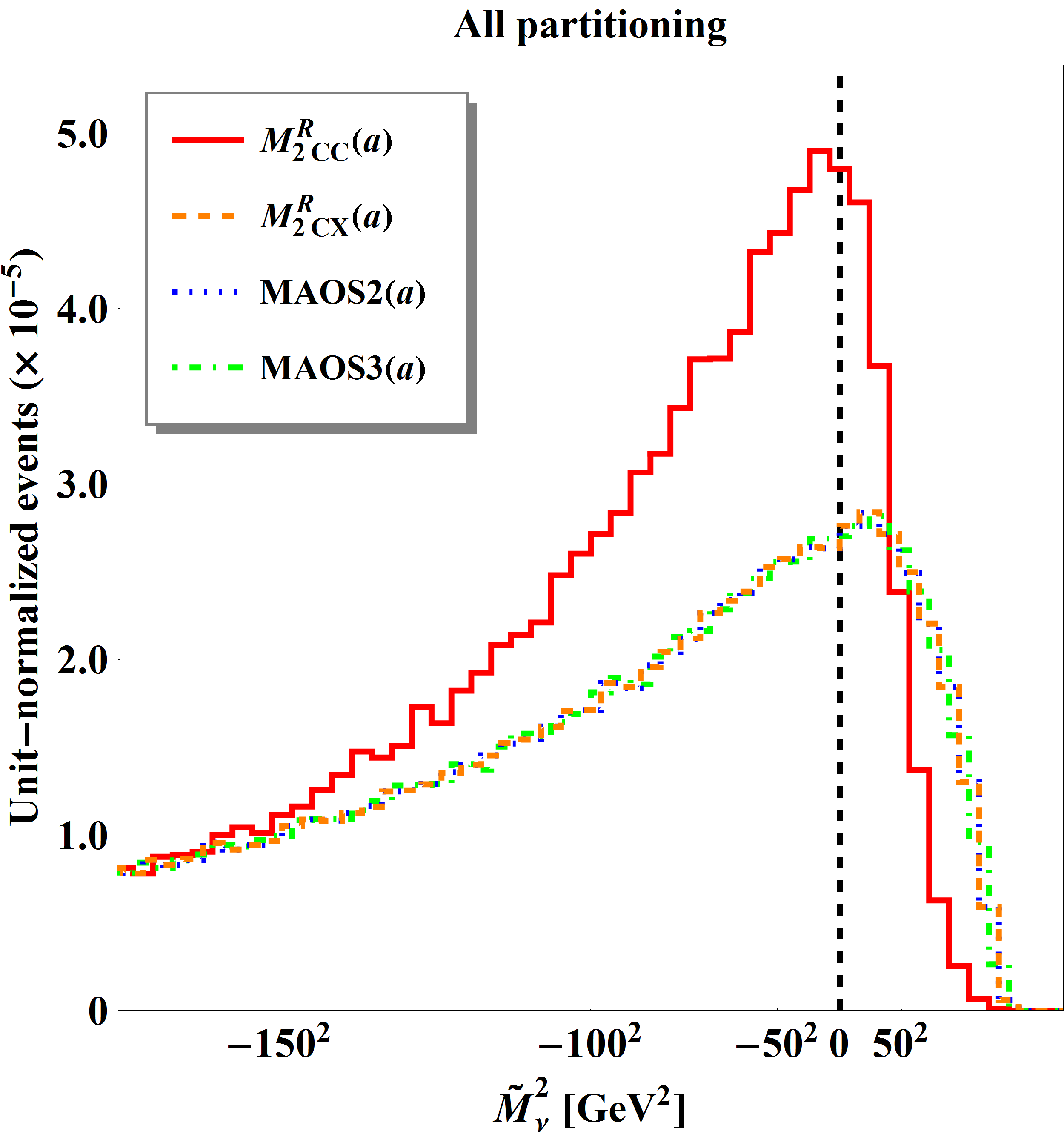
Finally, in Fig. 10 we revisit our results from Figs. 4 and 7 for the reconstructed neutrino mass-squared $\tilde{M}^{2}_{\nu}$. This time there is only a single method, MAOS1(a), which uses two mass inputs, and correspondingly, it is depicted in the left panel. The remaining four methods use a single input, the $W$-boson mass, and are shown in the right panel. Once again, in accordance with the theorem from Cho:2014naa , the distributions for $M_{2CX}(a)$ (the orange dashed line) and MAOS2(a) (the blue dotted line) are identical. The lack of unbalanced events in subsystem $(a)$ implies that the distributions corresponding to MAOS2(a) and MAOS3(a) are also the same. The remaining fourth distribution, based on $M_{2CC}(a)$ (the red solid line) is different, however, and appears to be the most promising for the purposes of a mass measurement of $\tilde{M}_{\nu}$.

In conclusion of this section, let us summarize our main result. We contrasted the MAOS and $M_{2}$ methods for invisible momentum reconstruction by examining their potential for a mass measurement of an unknown particle through a bump hunt. We analyzed each of the three subsystems in the event topology of Fig. 1 and found that the invisible momentum reconstruction offered by the $M_{2}$ class of variables is generally superior to MAOS — the reconstructed invariant mass peaks are more narrow and better localized. An additional theoretical advantage of the $M_{2}$ approach is that it is less ambiguous, as it always provides a unique ansatz for balanced events. In the next section we shall continue to investigate the $M_{2}$ approach in the most general case of the event topology from Fig. 1, where $A$, $B$ and $C$ are arbitrary new physics particles.

5 Applicability to BSM scenarios

Our discussion in the previous section was limited to the SM $t\bar{t}$ dilepton event topology. The dilepton $t\bar{t}$ example is appealing to an experimentalist mainly because we know it is present in the data and can be used as a toy playground for new physics searches Chatrchyan:2013boa ; CMS:2016kgk ; ATLAS:2012poa . Given that the ultimate goal of the LHC is to discover new physics and measure the new particle mass spectrum, in this section we shall abandon the $t\bar{t}$ example and instead consider the most general case of the event topology of Fig. 1, where the mass spectrum $(m_{A},m_{B},m_{C})$ is completely arbitrary, and not $(m_{t},m_{W},m_{\nu})$, as in the previous section. A concrete realization in SUSY is provided by the process (33) of stop production, in which the masses of the top squark, chargino and sneutrino are a priori unknown.

The main goal of this section will be to revisit the bump hunting mass measurement technique discussed previously and investigate how well it does in the general mass parameter space $(m_{A},m_{B},m_{C})$, away from our previous “study point” $(m_{t},m_{W},m_{\nu})$. Since the exact nature of the new physics particles $A$, $B$ and $C$ is unknown, in the simulations of this section we shall decay particles $A$ and $B$ by pure phase space. For concreteness, we shall continue to assume that particles $A$ are colored fermions produced similarly to top quarks. For fairness in comparing the sensitivity at different points in mass parameter space, it would be nice to fix the overall signal rate. An easy way to do this is to fix the mass (and hence the cross-section) of the heaviest particle $A$. In what follows we shall choose $m_{A}=500$ GeV; this has the additional benefit of reducing the dimensionality of the relevant mass parameter space to two. The masses of the two remaining particles will be varied as $m_{B}\in(0,m_{A})$ and $m_{C}\in(0,m_{B})$. We shall then investigate the sensitivity of the method as a function of $m_{B}$ and $m_{C}$.

Figure 11: An example of stop production (33) which works rather well. The mass spectrum is $m_{A}=500$ GeV, $m_{B}=300$ GeV, $m_{C}=200$ GeV. The top row shows the $M_{2CC}(ab)$ distribution (left panel), the corresponding reconstruction of the relative particle $B$ in the (ab) subsystem (middle panel), and their correlation (right panel). The bottom row shows the $M_{2CC}(b)$ distribution (left panel), the corresponding reconstruction of the relative particle $A$ in the (b) subsystem (middle panel), and their correlation (right panel). The dashed lines mark the true values of the particle masses in each case.

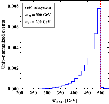
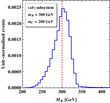
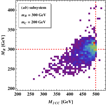
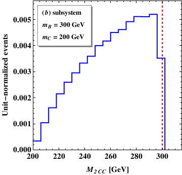
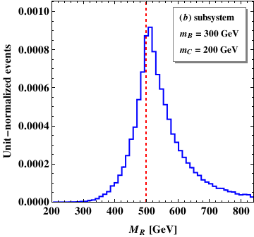
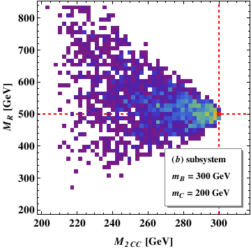
In Fig. 11 we revisit the main study point considered in Cho:2014naa , namely $m_{A}=500$ GeV, $m_{B}=300$ GeV, $m_{C}=200$ GeV. In the left panels we show the distributions of $M_{2CC}(ab)$ (upper row) and $M_{2CC}(b)$ (lower row), both made with the correct choice of $m_{C}$. We observe that both distributions peak very nicely at their kinematic endpoint, allowing a measurement of the corresponding mass ($m_{A}$ for the case of $M_{2CC}(ab)$ and $m_{B}$ for the case of $M_{2CC}(b)$) from either the peak of the distribution, or the location of the kinematic endpoint. For our purposes, however, we are mostly interested in using the invisible momentum ansatz for reconstructing the mass of the relative particle, namely $m_{B}$ for the case of $M_{2CC}(ab)$ and $m_{A}$ for the case of $M_{2CC}(b)$. This reconstruction is shown in the two middle panels of Fig. 11. We see that the reconstructed relative mass distributions have very sharp, well-defined peaks positioned very close to the true values of the masses, which are indicated by the vertical dashed lines. We conclude that for the particular study point shown in Fig. 11, the invisible momentum reconstruction is quite successful and the bump hunt measurement is very promising. For future reference, the two right panels in Fig. 11 then show the correlations between the two variables plotted in the left and middle panels of each row.

Figure 12: The same as Fig. 11, but for a study point which does not work as well: $m_{A}=500$ GeV, $m_{B}=450$ GeV, $m_{C}=50$ GeV.

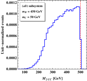
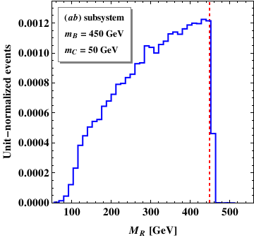
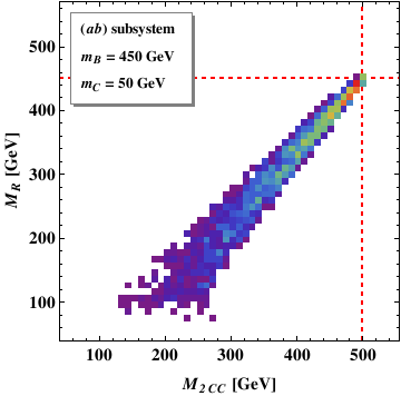
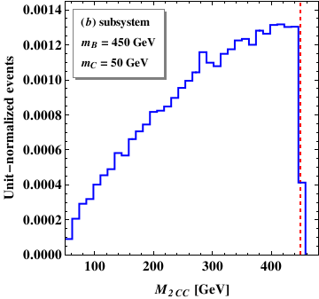
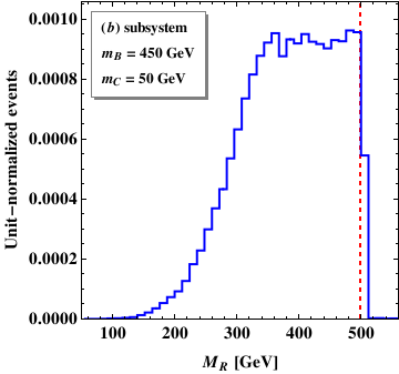
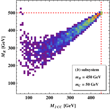
Fig. 12 presents the same results, but for a different study point, $m_{A}=500$ GeV, $m_{B}=450$ GeV, and $m_{C}=50$ GeV. The mass spectrum was judiciously chosen so that the shapes of the relevant kinematic distributions are adversely affected. For example, as shown in the upper left panel, the peak in the $M_{2CC}(ab)$ distribution is now much broader, extending significantly to the left (compare to the upper left panel in Fig. 11). Reconstructing the masses of the relative particles now appears to be a bit more problematic, as illustrated by the middle panels in Fig. 12 — in the upper row, the peak in the distribution of $m_{B}$ reconstructed with the invisible momenta from $M_{2CC}(ab)$, is very asymmetric. The lower middle panel shows an even worse situation: the distribution of $m_{C}$ reconstructed with the invisible momenta from $M_{2CC}(b)$ appears flat from $300$ GeV all the way to $500$ GeV, making the corresponding mass determination quite uncertain.

Fortunately, there exists a way to recover sensitivity. The basic idea can be understood from the correlation plots in the right panels of Fig. 12. Notice that the most populated bins are situated very close to the true values of the masses, $m_{B}=450$ GeV and $m_{A}=500$ GeV. The problem arises because of the appearance of the tail extending towards lower values of the reconstructed relative mass $M_{R}$, so that when we project this two-dimensional plot on the $y$-axis, the obtained distribution is skewed towards lower values of $M_{R}$ as well. This basic observation suggests the two possible solutions to the problem. First, instead of bump hunting on a one-dimensional histogram, one may target directly the most populated bins in the two-dimensional correlation plots shown in the right panels of Fig. 12 (note that this method would have also worked on our previous example shown in Fig. 11). The use of such two-dimensional correlation plots was previously suggested in order to detect the kinematic boundaries of the available phase space Costanzo:2009mq ; Burns:2009zi ; Matchev:2009iw ; Debnath:2015wra ; Debnath:2016mwb ; Debnath:2016gwz , while here we propose to use them in order to find the location of the highest density.

Figure 13: The effect of a preselection cut on the reconstructed relative mass distributions shown in the middle panel plots from Figs. 11, 12 and 15. The preselection cut is applied on the variable $M_{2CC}(ab)$ (upper row) or $M_{2CC}(b)$ (lower row). The left, middle and right plots correspond to the study points from Fig. 11, Fig. 12 and Fig. 15, respectively. Events are selected in the top 5% (red), top 10% (orange), top 20% (green) and top 50% of the allowed range for the $M_{2CC}$ variable.

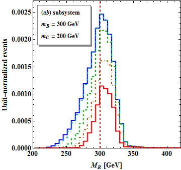
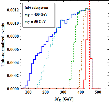
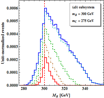
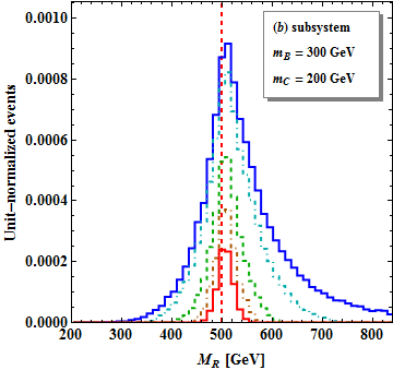
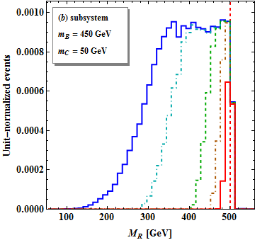
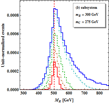
An alternative approach is based on the following observation. The right panels in Figs. 11 and 12 show that the correct value of the relative mass $M_{R}$ is obtained for events with extreme values of the $M_{2CC}$ kinematic variable plotted on the $x$-axis. In other words, the ansatz for the invisible momenta tends to work best for events near the $M_{2CC}$ kinematic endpoint (this was first pointed out in the context of MAOS reconstruction Cho:2008tj , and follows from the general principle that kinematic endpoints are attained at very special extreme momentum configurations Hinchliffe:1996iu ; Kersting:2009ne ; Matchev:2009fh ). Thus the precision of the one-dimensional bump hunting method will be recovered, if we simply apply a preselection cut on $M_{2CC}$ to eliminate the effect of the tail. Ideally, one would like to select only events which sit right at the $M_{2CC}$ kinematic endpoint, but such a severe cut may cause too large of a loss of statistics. This trade-off is illustrated in Fig. 13, which shows the effect of the preselection cut on the reconstructed relative mass distributions shown in the middle panel plots from Fig. 11 and 12. The preselection cut is applied on the corresponding $M_{2CC}$ variable from the $x$-axis of the scatter plots in the right panels of Figs. 11 and 12, $M_{2CC}(ab)$ (plots in the upper row) or $M_{2CC}(b)$ (plots in the lower row). The left (middle) plots correspond to the study point from Fig. 11 (Fig. 12). The middle plots in Fig. 13 nicely illustrate the benefit from the preselection cut — the unwanted events from the tail are removed and the mass bump is rendered more symmetric, and is now centered on the correct mass value for the relative particle. However, those benefits do come at a cost - the number of events in the mass bump is correspondingly reduced. (Note, however, the upper middle panel of Fig. 13, where the cut seems to cause no appreciable loss in statistics.) On the other hand, the left plots in Fig. 13 show that for our first study point from Fig. 11, the cut does not lead to a big improvement in the shape of the distribution, but this is because the shape was already very good to begin with, and thus a preselection cut would be unnecessary.

Figure 14: The fraction of events falling within the rightmost 5% of the allowed range for $M_{2CC}(ab)$ (left panel), $M_{2CC}(b)$ (middle panel) and $M_{2CC}(a)$ (right panel). The mass of $A$ is fixed at $m_{A}=500$ GeV, while $m_{B}$ and $m_{C}$ are varied as $m_{B}\in(0,m_{A})$ and $m_{C}\in(0,m_{B})$.

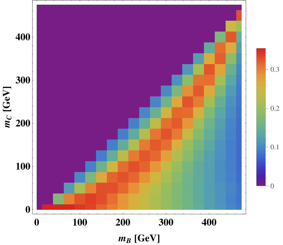
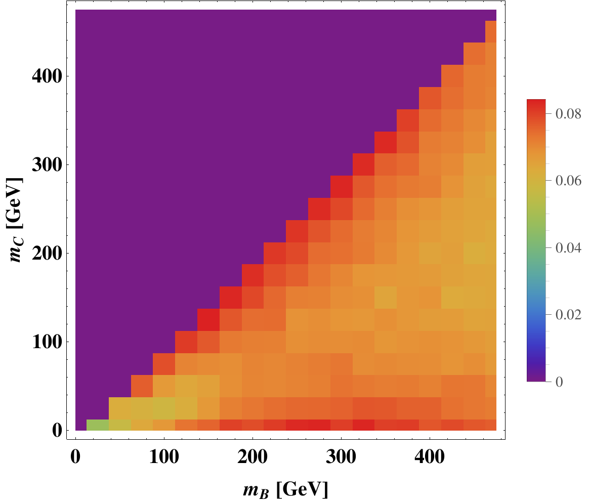
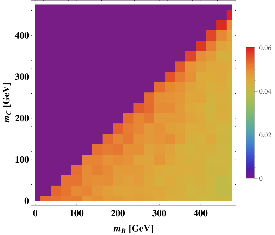
The loss of statistics observed in Fig. 13 as a result of the preselection cut suggests that a crucial issue for us to consider is the population of the $M_{2CC}$ bins near the upper kinematic endpoint. This is investigated in Fig. 14 as a function of the general mass parameter space $(m_{B},m_{C})$ for a fixed $m_{A}=500$ GeV. The figure shows results for each of the three subsystems: $(ab)$ in the left panel, $(b)$ in the middle panel, and $(a)$ in the right panel. For any given choice of $m_{B}$ and $m_{C}$, we take the allowed range for the corresponding $M_{2CC}$ variable, i.e., the difference between its upper and lower kinematic endpoints, and divide it into 20 equal size bins. Then the rainbow scale in Fig. 14 indicates the fraction of events which fell into the very last bin, i.e. in the upper 5% of the $M_{2CC}$ range, close to the upper kinematic endpoint.

Fig. 14 reveals that throughout the whole mass parameter space, the rightmost bin is very well populated in the case of the $(ab)$ subsystem, and less so in the case of the $(b)$ and $(a)$ subsystems. Given that invisible momentum reconstruction works best for events near the last bin, this suggests that variables based on the $(ab)$ subsystem have a certain advantage in terms of statistics and accuracy. Upon closer inspection of the left panel in Fig. 14, we find that the last bin is maximally populated if the mass spectrum satisfies the relation

$$m_{C}=\frac{m_{B}^{2}}{m_{A}},$$ (41)

whose physical meaning is the following — in the rest frame of particle $A_{i}$, particle $C_{i}$ remains at rest, while the visible particles $a_{i}$ and $b_{i}$ are back-to-back. The relation (41) was approximately satisfied for the study point in Fig. 11, where we had $m_{C}=200$ GeV and $m_{B}^{2}/m_{A}=180$ GeV. On the other hand, the study point in Fig. 12 was characterized by $m_{C}=50$ GeV and $m_{B}^{2}/m_{A}=405$ GeV, which significantly violated (41) by $m_{C}$ being too low. Note that the relation (41) is scale invariant, i.e., the result does not change if we inflate all masses by the same constant factor. We checked this with explicit simulations, and verified that much heavier spectra which satisfy (41), continue to exhibit nice reconstructed peaks and vice versa.

In conclusion of this section, we shall test the prediction (41) by choosing a point for which $m_{C}$ is too high. Let us again take $m_{A}=500$ GeV and $m_{B}=300$ GeV, as in Fig. 11, only now increase the value of $m_{C}$ to $275$ GeV, well above the prediction from (41). The result is shown in Fig. 15.

Figure 15: The same as Fig. 12, but for an example with a relatively high value of $m_{C}$: $m_{A}=500$ GeV, $m_{B}=300$ GeV, $m_{C}=275$ GeV.

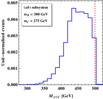
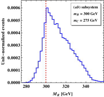
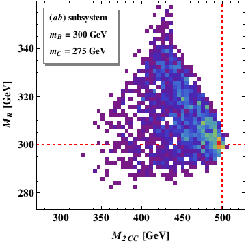
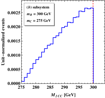
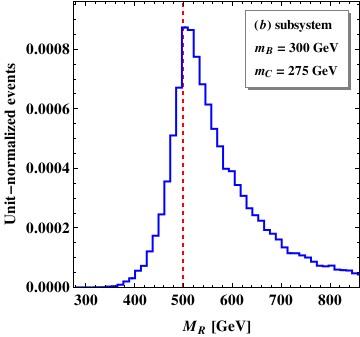
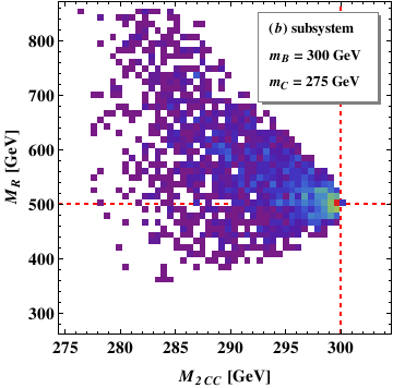
The upper left panel shows that, as designed, the events near the $M_{2CC}(ab)$ kinematic endpoint are depleted, and the peak of the $M_{2CC}(ab)$ distribution has now moved to lower values, away from the kinematic endpoint. The right panels again exhibit tails, only this time the tails curl up towards higher values of the reconstructed relative mass, leading to an overestimate of the mass — the bulk of the $M_{R}$ distributions in the middle panels extend above the nominal mass of the respective parent particle. However, these problems can be again overcome by the two techniques considered earlier — applying a preselection cut on events near the $M_{2CC}(ab)$ kinematic endpoint (see the right panels in Fig. 13), or directly targeting the most populated bins in the two-dimensional correlation plots in the right panels of Fig. 15.

6 Conclusions and outlook

Understanding the kinematics of events with missing transverse momentum at hadron colliders like the LHC is an important task, since many new physics models have collider signatures with dark matter particles and/or neutrinos, whose individual momenta and energies are not measured in the detector. The two traditional approaches for analyzing such events are 1) where available, use a sufficient number of on-shell constraints to solve for the invisible momenta exactly; and 2) use variables which do not require any actual knowledge of the individual invisible momenta. However, recently several prescriptions for assigning approximate values to the individual invisible momenta have emerged. The main goal of this paper was to advertise the existence of a large number of such ansatze (3) and demonstrate their usefulness for the purposes of a mass measurement through a bump hunt. Our specific points are the following.

• Many different ansatze are possible. Quite often, any given prescription for assigning invisible momenta has many different variations, as we demonstrated in Sections 3.1 and 3.2, where we defined 12 versions of the MAOS method and 18 versions of the $M_{2}$ method, respectively, in the case of the dilepton $t\bar{t}$ event topology.

• The $M_{2}$ class of variables automatically provides ansatze for the longitudinal components of the invisible momenta. As discussed in Sections 3 and 4, the important advantage of the $M_{2}$ class of (3+1)-dimensional invariant mass variables is that they automatically provide values for the longitudinal components of the invisible momenta, without any need for additional mass inputs. In that sense, they are on the same theoretical footing as the MAOS2 and MAOS3 versions of the MAOS method, but significantly outperform them in the presence of the relative mass constraint (29).

• The $M_{2}$-based reconstruction of invisible momenta is superior to the MAOS schemes. In this paper, we compared the performance of the two methods using the example of a bump hunt mass measurement. Our results in Sec. 4.3 showed that the invisible momenta found by the $M_{2}$ class of variables generally lead to a better determination of the new particle masses.

• Software support. With the release of the public code Optimass Cho:2015laa which is capable of computing the on-shell constrained $M_{2}$ variables for general event topologies, the corresponding ansatze for the invisible momenta are also readily available and can be used for phenomenological studies similar to the one in this paper. For example, one could imagine spin measurements as in Refs. Cho:2008tj ; Cheng:2010yy ; Guadagnoli:2013xia , or designing procedures for reducing the combinatorial background Rajaraman:2010hy ; Baringer:2011nh ; Choi:2011ys ; us .

• Sensitivity study throughout the mass parameter space. In Section 5 we investigated the precision of the invisible momentum reconstruction throughout the full mass parameter space, and identified the regions where sensitivity can be lost. We proposed to mitigate the problem by either studying the 2D correlations of the reconstructed mass and the $M_{2}$ variable, or by applying a preselection cut on the $M_{2}$ variable in order to only select events near its kinematic endpoint.