Resistance metric, and spectral asymptotics, on the graph of the Weierstrass function

Sorbonne Universités, UPMC Univ Paris 06

CNRS, UMR 7598, Laboratoire Jacques-Louis Lions, 4, place Jussieu 75005, Paris, France

1 Introduction

Following our work on the graph of the Weierstrass function [5], in the spirit of those of J. Kigami  [1], [2], and [3], [29], which enabled us to build a Laplacian on the aforementioned graph, it was natural to go further and give the related explicit resistance metric. In doing so, we made calculations that directly enable one to obtain the box dimension of the graph, in a simpler way than [6]or [7].

The aim of this work is twofold. We had a special interest in the study of the spectral properties of the Laplacian. In [5], we have given the explicit the spectrum on the graph of the Weierstrass function. In the case of Laplacians on post-critically finite fractals, previous works, by J. Kigami and M. Lapidus [10], and R. S. Strichartz [29], make the link between resistance metric, and asymptotic properties of the spectrum of the Laplacian, by means of an analoguous of Weyl’s formula.

So we asked ourselves wether those results were still valid, for the graph of the Weierstrass function.

2 Framework of the study

In this section, we recall results that are developed in [5].

Notation.

In the following, $\lambda$ and $N_{b}$ are two real numbers such that:

$$0<\lambda<1\quad,\quad N_{b}\,\in\,{\mathbb{N}}\quad\text{and}\quad\lambda\,N_{b}>1$$

We will consider the ($1-$periodic) Weierstrass function ${\cal W}$, defined, for any real number $x$, by:

$${\cal W}(x)=\displaystyle\sum_{n=0}^{+\infty}\lambda^{n}\,\cos\left(2\,\pi\,N_{b}^{n}\,x\right)$$

We place ourselves, in the sequel, in the Euclidean plane of dimension 2, referred to a direct orthonormal frame. The usual Cartesian coordinates are $(x,y)$.

The restriction $\Gamma_{\cal W}$ to $[0,1[\times{\mathbb{R}}$, of the graph of the Weierstrass function, is approximated by means of a sequence of graphs, built through an iterative process. To this purpose, we introduce the iterated function system of the family of $C^{\infty}$ contractions from ${\mathbb{R}}^{2}$ to ${\mathbb{R}}^{2}$:

$$\left\{T_{0},...,T_{N_{b}-1}\right\}$$

where, for any integer $i$ belonging to $\left\{0,...,N_{b}-1\right\}$, and any $(x,y)$ of ${\mathbb{R}}^{2}$:

$$T_{i}(x,y)=\left(\displaystyle\frac{x+i}{N_{b}},\lambda\,y+\cos\left(2\,\pi\,\left(\frac{x+i}{N_{b}}\right)\right)\right)$$

Property 2.1.

$$\Gamma_{\cal W}=\underset{i=0}{\overset{N_{b}-1}{\bigcup}}\,T_{i}(\Gamma_{\cal W})$$

Definition 2.1.

For any integer $i$ belonging to $\left\{0,...,N_{b}-1\right\}$, let us denote by:

$$P_{i}=(x_{i},y_{i})=\left(\displaystyle\frac{i}{N_{b}-1},\displaystyle\frac{1}{1-\lambda}\,\cos\left(\displaystyle\frac{2\,\pi\,i}{N_{b}-1}\right)\right)$$

the fixed point of the contraction $T_{i}$.

We will denote by $V_{0}$ the ordered set (according to increasing abscissa), of the points:

$$\left\{P_{0},...,P_{N_{b}-1}\right\}$$

The set of points $V_{0}$, where, for any $i$ of $\left\{0,...,N_{b}-2\right\}$, the point $P_{i}$ is linked to the point $P_{i+1}$, constitutes an oriented graph (according to increasing abscissa)), that we will denote by $\Gamma_{{\cal W}_{0}}$. $V_{0}$ is called the set of vertices of the graph $\Gamma_{{\cal W}_{0}}$.

For any natural integer $m$, we set:

$$V_{m}=\underset{i=0}{\overset{N_{b}-1}{\bigcup}}\,T_{i}\left(V_{m-1}\right)$$

The set of points $V_{m}$, where two consecutive points are linked, is an oriented graph (according to increasing abscissa), which we will denote by $\Gamma_{{\cal W}_{m}}$. $V_{m}$ is called the set of vertices of the graph $\Gamma_{{\cal W}_{m}}$. We will denote, in the sequel, by

$${\cal N}^{\cal S}_{m}=2\,N_{b}^{m}+N_{b}-2$$

the number of vertices of the graph $\Gamma_{{\cal W}_{m}}$, and we will write:

$$V_{m}=\left\{{\cal S}_{0}^{m},{\cal S}_{1}^{m},\ldots,{\cal S}_{{\cal N}_{m}-1}^{m}\right\}$$

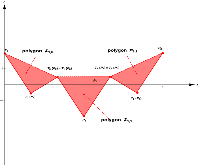
Figure 1: The polygons ${\cal P}_{1,0}$, ${\cal P}_{1,1}$, ${\cal P}_{1,2}$, in the case where $\lambda=\displaystyle\frac{1}{2}$, and $N_{b}=3$.

Figure 2: The graphs $\Gamma_{{\cal W}_{0}}$ (in green),  $\Gamma_{{\cal W}_{1}}$ (in red), $\Gamma_{{\cal W}_{2}}$ (in orange), $\Gamma_{{\cal W}}$ (in cyan), in the case where $\lambda=\displaystyle\frac{1}{2}$, and $N_{b}=3$.

Definition 2.2.

Consecutive vertices on the graph $\Gamma_{\cal W}$

Two points $X$ et $Y$ de $\Gamma_{{\cal W}}$ will be called consecutive vertices of the graph $\Gamma_{\cal W}$ if there exists a natural integer $m$, and an integer $j$ of $\left\{0,...,N_{b}-2\right\}$, such that:

$$X=\left(T_{i_{1}}\circ\ldots\circ T_{i_{m}}\right)(P_{j})\quad\text{et}\quad Y=\left(T_{i_{1}}\circ\ldots\circ T_{i_{m}}\right)(P_{j+1})\qquad\left\{i_{1},\ldots,i_{m}\right\}\,\in\,\left\{0,...,N_{b}-1\right\}^{m}$$

or:

$$X=\left(T_{i_{1}}\circ T_{i_{2}}\circ\ldots\circ T_{i_{m}}\right)\left(P_{N_{b}-1}\right)\quad\text{et}\quad Y=\left(T_{i_{1}+1}\circ T_{i_{2}}\ldots\circ T_{i_{m}}\right)(P_{0})$$

Definition 2.3.

For any natural integer $m$, the ${\cal N}^{\cal S}_{m}$ consecutive vertices of the graph $\Gamma_{{\cal W}_{m}}$ are, also, the vertices of $N_{b}^{m}$ simple polygons ${\cal P}_{m,j}$, $0\leqslant j\leqslant N_{b}^{m}-1$, with $N_{b}$ sides. For any integer $j$ such that $0\leqslant j\leqslant N_{b}^{m}-1$, one obtains each polygon by linking the point number $j$ to the point number $j+1$ if $j=i\,\text{mod }N_{b}$, $0\leqslant i\leqslant N_{b}-2$, and the point number $j$ to the point number $j-N_{b}+1$ if $j=-1\,\text{mod }N_{b}$. These polygons generate a Borel set of ${\mathbb{R}}^{2}$.

Definition 2.4.

Polygonal domain delimited by the graph $\Gamma_{{\cal W}_{m}}$, $m\,\in\,{\mathbb{N}}$

For any natural integer $m$, well call polygonal domain delimited by the graph $\Gamma_{{\cal W}_{m}}$, and denote by ${\cal D}\left(\Gamma_{{\cal W}_{m}}\right)$, the reunion of the $N_{b}^{m}$ polygons ${\cal P}_{m,j}$, $0\leqslant j\leqslant N_{b}^{m}-1$, with $N_{b}$ sides.

Definition 2.5.

Polygonal domain delimited by the graph $\Gamma_{{\cal W}}$

We will call polygonal domain delimited by the graph $\Gamma_{{\cal W}}$, and denote by ${\cal D}\left(\Gamma_{{\cal W}}\right)$, the limit:

$${\cal D}\left(\Gamma_{{\cal W}}\right)=\displaystyle\lim_{n\to+\infty}{\cal D}\left(\Gamma_{{\cal W}_{m}}\right)$$

Definition 2.6.

Word, on the graph $\Gamma_{\cal W}$

Let $m$ be a strictly positive integer. We will call number-letter any integer ${\cal M}_{i}$ of $\left\{0,\ldots,N_{b}-1\right\}$, and word of length $|{\cal M}|=m$, on the graph $\Gamma_{\cal W}$, any set of number-letters of the form:

$${\cal M}=\left({\cal M}_{1},\ldots,{\cal M}_{m}\right)$$

We will write:

$$T_{\cal M}=T_{{\cal M}_{1}}\circ\ldots\circ T_{{\cal M}_{m}}$$

Definition 2.7.

Edge relation, on the graph $\Gamma_{\cal W}$

Given a natural integer $m$, two points $X$ and $Y$ of $\Gamma_{{\cal W}_{m}}$ will be called adjacent if and only if $X$ and $Y$ are two consecutive vertices of $\Gamma_{{\cal W}_{m}}$. We will write:

$$X\underset{m}{\sim}Y$$

This edge relation ensures the existence of a word ${\cal M}=\left({\cal M}_{1},\ldots,{\cal M}_{m}\right)$ of length $m$, such that $X$ and $Y$ both belong to the iterate:

$$T_{\cal M}\,V_{0}=\left(T_{{\cal M}_{1}}\circ\ldots\circ T_{{\cal M}_{m}}\right)\,V_{0}$$

Given two points $X$ and $Y$ of the graph $\Gamma_{\cal W}$, we will say that $X$ and $Y$ are adjacent if and only if there exists a natural integer $m$ such that:

$$X\underset{m}{\sim}Y$$

Proposition 2.2.

Adresses, on the graph of the Weierstrass function

Given a strictly positive integer $m$, and a word ${\cal M}=\left({\cal M}_{1},\ldots,{\cal M}_{m}\right)$ of length $m\,\in\,{\mathbb{N}}^{\star}$, on the graph $\Gamma_{{\cal W}_{m}}$, for any integer $j$ of $\left\{1,...,N_{b}-2\right\}$, any $X=T_{\cal M}(P_{j})$ de $V_{m}\setminus V_{0}$, i.e. distinct from one of the $N_{b}$ fixed point $P_{i}$,  $0\leqslant i\leqslant N_{b}-1$, has exactly two adjacent vertices, given by:

$$T_{\cal M}(P_{j+1})\quad\text{et}\quad T_{\cal M}(P_{j-1})$$

where:

$$T_{\cal M}=T_{{\cal M}_{1}}\circ\ldots\circ T_{{\cal M}_{m}}$$

By convention, the adjacent vertices of $T_{{\cal M}}(P_{0})$ are $T_{{\cal M}}(P_{1})$ and $T_{{\cal M}}(P_{N_{b}-1})$, those of $T_{{\cal M}}(P_{N_{b}-1})$, $T_{{\cal M}}(P_{N_{b}-2})$ and $T_{{\cal M}}(P_{0})$ .

Definition 2.8.

$m^{th}-$order subcell, $m\,\in\,{\mathbb{N}}^{\star}$, related to a pair of points of the graph $\Gamma_{\cal W}$

Given a strictly positive integer $m$, and two points $X$ and $Y$ of $V_{m}$ such that $X\underset{m}{\sim}Y$, we will call $m^{th}-$order subcell, related to the pair of points $(X,Y)$, the polygon, the vertices of which are $X$, $Y$, and the intersection points of the edge between the vertices at the extremities of the polygon, i.e. the respective intersection points of polygons of the type ${\cal P}_{m,j-1}$ and ${\cal P}_{m,j}$, $1\leqslant j\leqslant N_{b}^{m}-1$, on the one hand, and of the type ${\cal P}_{m,j}$ and ${\cal P}_{m,j+1}$, $0\leqslant j\leqslant N_{b}^{m}-2$, on the other hand.

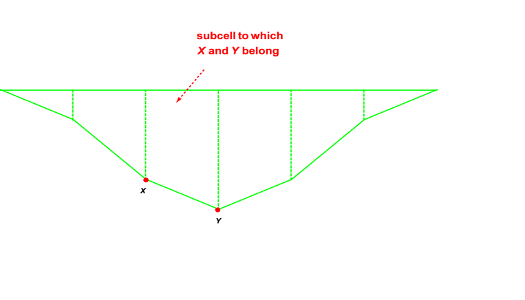
Figure 3: A $m^{th}-$order subcell, in the case where $\lambda=\displaystyle\frac{1}{2}$, and $N_{b}=7$.

Notation.

For any integer $j$ belonging to $\left\{0,...,N_{b}-1\right\}$, any natural integer $m$, and any word $\cal M$ of length $m$, we set:

$$\begin{array}[]{ccc}T_{\cal M}\left(P_{j}\right)&=&\left(x\left(T_{\cal M}\left(P_{j}\right)\right),y\left(T_{\cal M}\left(P_{j}\right)\right)\right)\end{array}\quad,\quad\begin{array}[]{ccc}T_{\cal M}\left(P_{j+1}\right)&=&\left(x\left(T_{\cal M}\left(P_{j+1}\right)\right),y\left(T_{\cal M}\left(P_{j+1}\right)\right)\right)\end{array}$$

$$L_{m}=x\left(T_{\cal M}\left(P_{j+1}\right)\right)-x\left(T_{\cal M}\left(P_{j}\right)\right)=\displaystyle\frac{1}{(N_{b}-1)\,N_{b}^{m}}$$

Proposition 2.3.

An upper bound and lower bound, for the box-dimension of the graph $\Gamma_{\cal W}$

For any integer $j$ belonging to $\left\{0,1,\ldots,N_{b}-2\right\}$, each natural integer $m$, and each word $\cal M$ of length $m$, let us consider the rectangle, the width of which is:

$$L_{m}=x\left(T_{\cal M}\left(P_{j+1}\right)\right)-x\left(T_{\cal M}\left(P_{j}\right)\right)=\displaystyle\frac{1}{(N_{b}-1)\,N_{b}^{m}}$$

and height $|h_{j,m}|$, such that the points $T_{\cal M}\left(P_{j+1}\right)$ and $T_{\cal M}\left(P_{j+1}\right)$ are two vertices of this rectangle.
Then:

$$L_{m}^{2-D_{\cal W}}\,(N_{b}-1)^{2-D_{\cal W}}\,\left|\left\{\displaystyle\frac{2}{1-\lambda}\,\displaystyle\min_{0\leqslant j\leqslant N_{b}-1}\sin\left(\displaystyle\frac{\pi\,(2\,j+1)}{N_{b}-1}\right)-\displaystyle\frac{\pi}{N_{b}\,(N_{b}-1)\,\left(\lambda\,N_{b}-1\right)}\right\}\right|\leqslant|h_{j,m}|$$

and:

$$|h_{j,m}|\leqslant\eta_{2-D_{\cal W}}\,L_{m}^{2-D_{\cal W}}$$

where the real constant $\eta_{2-D_{\cal W}}$ is given by :

$$\eta_{2-D_{\cal W}}=2\,\pi^{2}\,(N_{b}-1)^{2-D_{\cal W}}\,\left\{\displaystyle\frac{(2\,N_{b}-1)\,\lambda\,(N_{b}^{2}-1)}{(N_{b}-1)^{2}\,(1-\lambda)\,(\lambda\,N_{b}^{2}-1)}+\displaystyle\frac{2\,N_{b}}{(\lambda\,N_{b}^{2}-1)\,(\lambda\,N_{b}^{3}-1)}\right\}$$

There exists thus a positive constant

$$C=\displaystyle\max\,\left\{\,(N_{b}-1)^{2-D_{\cal W}}\,\left|\left\{\displaystyle\frac{2}{1-\lambda}\,\displaystyle\min_{0\leqslant j\leqslant N_{b}-1}\sin\left(\displaystyle\frac{\pi\,(2\,j+1)}{N_{b}-1}\right)-\displaystyle\frac{\pi}{N_{b}\,(N_{b}-1)\,\left(\lambda\,N_{b}-1\right)}\right\}\right|,\eta_{2-D_{\cal W}}\right\}$$

such that the graph $\Gamma_{\cal W}$ on $L_{m}$ can be covered by at least and at most:

$$N_{m}\,\left\{C\,\left(\displaystyle\frac{L_{m}}{N_{m}}\right)^{1-D_{\cal W}}+1\right\}=C\,L_{m}^{1-D_{\cal W}}\,N_{m}^{D_{\cal W}}+N_{m}$$

squares, the side length of which is $\displaystyle\frac{L_{m}}{N_{m}}$.

Proof.

For any pair of integers $(i_{m},j)$ of $\left\{0,...,N_{b}-2\right\}^{2}$:

$$\begin{array}[]{ccc}T_{i_{m}}\left(P_{j}\right)&=&\left(\displaystyle\frac{x_{j}+i_{m}}{N_{b}},\lambda\,y_{j}+\cos\left(2\,\pi\,\left(\frac{x_{j}+i_{m}}{N_{b}}\right)\right)\right)\end{array}$$

For any pair of integers  $(i_{m},i_{m-1},j)$ of $\left\{0,...,N_{b}-2\right\}^{3}$:

$$\begin{array}[]{ccc}T_{i_{m-1}}\left(T_{i_{m}}\left(P_{j}\right)\right)&=&\left(\displaystyle\frac{\frac{x_{j}+{i_{m}}}{N_{b}}+i_{m-1}}{N_{b}},\lambda^{2}\,y_{j}+\lambda\,\cos\left(2\,\pi\,\left(\frac{x_{j}+{i_{m}}}{N_{b}}\right)\right)+\cos\left(2\,\pi\,\left(\frac{\frac{x_{j}+{i_{m}}}{N_{b}}+i_{m-1}}{N_{b}}\right)\right)\right)\\ \\ &=&\left(\displaystyle\frac{x_{j}+{i_{m}}}{N_{b}^{2}}+\displaystyle\frac{i_{m-1}}{N_{b}},\lambda^{2}\,y_{j}+\lambda\,\cos\left(2\,\pi\,\left(\frac{x_{j}+{i_{m}}}{N_{b}}\right)\right)+\cos\left(2\,\pi\,\left(\displaystyle\frac{x_{j}+{i_{m}}}{N_{b}^{2}}+\displaystyle\frac{i_{m-1}}{N_{b}}\right)\right)\right)\\ \end{array}$$

For any pair of integers $(i_{m},i_{m-1},i_{m-2},j)$ of $\left\{0,...,N_{b}-2\right\}^{4}$:

$$\begin{array}[]{ccc}T_{i_{m-2}}\left(T_{i_{m-1}}\left(T_{i_{m}}\left(P_{j}\right)\right)\right)&=&\bigg{(}\displaystyle\frac{x_{j}+{i_{m}}}{N_{b}^{3}}+\displaystyle\frac{i_{m-1}}{N_{b}^{2}}+\displaystyle\frac{i_{m-2}}{N_{b}},\\ &&\lambda^{3}\,y_{j}+\lambda^{2}\,\cos\left(2\,\pi\,\left(\frac{x_{j}+i_{m}}{N_{b}}\right)\right)\\ &&+\lambda\,\cos\left(2\,\pi\,\left(\displaystyle\frac{x_{j}+{i_{m}}}{N_{b}^{2}}+\displaystyle\frac{i_{m-1}}{N_{b}}\right)\right)+\cos\left(2\,\pi\,\left(\displaystyle\frac{x_{j}+{i_{m}}}{N_{b}^{3}}+\displaystyle\frac{i_{m-1}}{N_{b}^{2}}+\displaystyle\frac{i_{m-2}}{N_{b}}\right)\right)\bigg{)}\end{array}$$

Given a strictly positive integer $m$, and two points $X$ and $Y$ of $V_{m}$ such that:

$$X\underset{m}{\sim}Y$$

there exists a word $\cal M$ of length $|{\cal M}|=m$, on the graph $\Gamma_{\cal W}$, and an integer $j$ of $\left\{0,...,N_{b}-2\right\}^{2}$, such that:

$$X=T_{\cal M}\left(P_{j}\right)\quad,\quad Y=T_{\cal M}\left(P_{j+1}\right)$$

Let us write $T_{\cal M}$ under the form:

$$T_{\cal M}=T_{i_{m}}\circ T_{i_{m-1}}\circ\ldots\circ T_{i_{1}}$$

where $(i_{1},\ldots,i_{m})\,\in\,\left\{0,...,N_{b}-1\right\}^{m}$.

One has then:

$$x\left(T_{\cal M}\left(P_{j}\right)\right)=\displaystyle\frac{x_{j}}{N_{b}^{m}}+\displaystyle\sum_{k=1}^{m}\frac{i_{k}}{N_{b}^{k}}\quad,\quad x\left(T_{\cal M}\left(P_{j+1}\right)\right)=\displaystyle\frac{x_{j+1}}{N_{b}^{m}}+\displaystyle\sum_{k=1}^{m}\frac{i_{k}}{N_{b}^{k}}$$

and:

$$\left\{\begin{array}[]{ccc}y\left(T_{\cal M}\left(P_{j}\right)\right)&=&\lambda^{m}\,y_{j}+\displaystyle\sum_{k=1}^{m}\lambda^{m-k}\,\cos\left(2\,\pi\,\left(\displaystyle\frac{x_{j}}{N_{b}^{k}}+\displaystyle\sum_{\ell=0}^{k}\frac{i_{m-\ell}}{N_{b}^{k-\ell}}\right)\right)\\ \\ y\left(T_{\cal M}\left(P_{j+1}\right)\right)&=&\lambda^{m}\,y_{j+1}+\displaystyle\sum_{k=1}^{m}\lambda^{m-k}\,\cos\left(2\,\pi\,\left(\displaystyle\frac{x_{j+1}}{N_{b}^{k}}+\displaystyle\sum_{\ell=0}^{k}\frac{i_{m-\ell}}{N_{b}^{k-\ell}}\right)\right)\end{array}\right.$$

This leads to:

$$\begin{array}[]{ccc}h_{j,m}-\lambda^{m}\,\left(y_{j+1}-y_{j}\right)&=&\displaystyle\sum_{k=1}^{m}\lambda^{m-k}\,\left\{\cos\left(2\,\pi\,\left(\displaystyle\frac{x_{j+1}}{N_{b}^{k}}+\displaystyle\sum_{\ell=0}^{k}\frac{i_{m-\ell}}{N_{b}^{k-\ell}}\right)\right)-\cos\left(2\,\pi\,\left(\displaystyle\frac{x_{j}}{N_{b}^{k}}-\displaystyle\sum_{\ell=0}^{k}\frac{i_{m-\ell}}{N_{b}^{k-\ell}}\right)\right)\right\}\\ \\ \\ &=&-2\displaystyle\sum_{k=1}^{m}\lambda^{m-k}\,\sin\left(\pi\,\left(\displaystyle\frac{x_{j+1}-x_{j}}{N_{b}^{k}}\right)\right)\,\sin\left(2\,\pi\,\left(\displaystyle\frac{x_{j+1}+x_{j}}{2\,N_{b}^{k}}+\displaystyle\sum_{\ell=0}^{k}\frac{i_{m-\ell}}{N_{b}^{k-\ell}}\right)\right)\\ \\ \\ \end{array}$$

Taking into account:

$$\begin{array}[]{ccc}\lambda^{m}\,\left(y_{j+1}-y_{j}\right)&=&\displaystyle\frac{\lambda^{m}}{1-\lambda}\,\left(\cos\left(\displaystyle\frac{2\,\pi\,(j+1)}{N_{b}-1}\right)-\cos\left(\displaystyle\frac{2\,\pi\,j}{N_{b}-1}\right)\right)\\ &=&-2\,\displaystyle\frac{\lambda^{m}}{1-\lambda}\,\sin\left(\displaystyle\frac{\pi}{N_{b}-1}\right)\,\sin\left(\displaystyle\frac{\pi\,(2\,j+1)}{N_{b}-1}\right)\\ \end{array}$$

one has:

$$\begin{array}[]{ccc}h_{j,m}+2\,\displaystyle\frac{\lambda^{m}}{1-\lambda}\,\sin\left(\displaystyle\frac{\pi}{N_{b}-1}\right)\,\sin\left(\displaystyle\frac{\pi\,(2\,j+1)}{N_{b}-1}\right)&=&-2\,\displaystyle\sum_{k=1}^{m}\lambda^{m-k}\,\sin\left(\displaystyle\frac{\pi}{N_{b}^{k+1}\,(N_{b}-1)}\right)\,\sin\left(\displaystyle\frac{\pi\,(2\,j+1)}{N_{b}^{k+1}\,(N_{b}-1)}+2\,\pi\,\displaystyle\sum_{\ell=0}^{k}\frac{i_{m-\ell}}{N_{b}^{k-\ell}}\right)\\ \end{array}$$

Thus:

$$\begin{array}[]{ccc}\left|y\left(T_{\cal M}\left(P_{j}\right)\right)-y\left(T_{\cal M}\left(P_{j+1}\right)\right)-2\,\displaystyle\frac{\lambda^{m}}{1-\lambda}\,\sin\left(\displaystyle\frac{\pi}{N_{b}-1}\right)\,\sin\left(\displaystyle\frac{\pi\,(2\,j+1)}{N_{b}-1}\right)\right|&\leqslant&\displaystyle\sum_{k=1}^{m}\displaystyle\frac{2\,\pi\,\lambda^{m-k}}{N_{b}^{k+1}\,(N_{b}-1)}\\ &=&\displaystyle\frac{\pi\,\lambda^{m}\,\left(1-\frac{1}{\lambda^{m}\,N_{b}^{m}}\right)}{\lambda\,N_{b}\,N_{b}\,(N_{b}-1)\,\left(1-\frac{1}{\lambda\,N_{b}}\right)}\\ &\leqslant&\displaystyle\frac{\pi\,\lambda^{m}}{N_{b}\,(N_{b}-1)\,\left(\lambda\,N_{b}-1\right)}\\ \\ \\ \end{array}$$

which leads to:

$$\begin{array}[]{ccc}y\left(T_{\cal M}\left(P_{j}\right)\right)-y\left(T_{\cal M}\left(P_{j+1}\right)\right)&\geqslant&2\,\displaystyle\frac{\lambda^{m}}{1-\lambda}\,\sin\left(\displaystyle\frac{\pi}{N_{b}-1}\right)\,\sin\left(\displaystyle\frac{\pi\,(2\,j+1)}{N_{b}-1}\right)-\displaystyle\frac{\pi\,\lambda^{m}}{N_{b}\,(N_{b}-1)\,\left(\lambda\,N_{b}-1\right)}\\ \\ \\ \end{array}$$

or:

$$\begin{array}[]{ccc}y\left(T_{\cal M}\left(P_{j+1}\right)\right)-y\left(T_{\cal M}\left(P_{j}\right)\right)&\geqslant&2\,\displaystyle\frac{\lambda^{m}}{1-\lambda}\,\sin\left(\displaystyle\frac{\pi}{N_{b}-1}\right)\,\sin\left(\displaystyle\frac{\pi\,(2\,j+1)}{N_{b}-1}\right)-\displaystyle\frac{\pi\,\lambda^{m}}{N_{b}\,(N_{b}-1)\,\left(\lambda\,N_{b}-1\right)}\\ \\ \\ \end{array}$$

Due to the symmetric roles played by $T_{\cal M}\left(P_{j}\right)$ and $T_{\cal M}\left(P_{j+1}\right)$, one may only consider the case when:

$$\begin{array}[]{ccccc}y\left(T_{\cal M}\left(P_{j}\right)\right)-y\left(T_{\cal M}\left(P_{j+1}\right)\right)&\geqslant&2\,\displaystyle\frac{\lambda^{m}}{1-\lambda}\,\sin\left(\displaystyle\frac{\pi}{N_{b}-1}\right)\,\sin\left(\displaystyle\frac{\pi\,(2\,j+1)}{N_{b}-1}\right)-\displaystyle\frac{\pi\,\lambda^{m}}{N_{b}\,(N_{b}-1)\,\left(\lambda\,N_{b}-1\right)}&\geqslant&0\\ &\geqslant&\lambda^{m}\,\left\{\displaystyle\frac{2}{1-\lambda}\,\displaystyle\min_{0\leqslant j\leqslant N_{b}-1}\sin\left(\displaystyle\frac{\pi\,(2\,j+1)}{N_{b}-1}\right)-\displaystyle\frac{\pi}{N_{b}\,(N_{b}-1)\,\left(\lambda\,N_{b}-1\right)}\right\}\\ \\ \\ \end{array}$$

The predominant term is thus:

$$\lambda^{m}=e^{m\,(D_{\cal W}-2)\,\ln N_{b}}=N_{b}^{m\,(D_{\cal W}-2)}=L_{m}^{2-D_{\cal W}}\,(N_{b}-1)^{2-D_{\cal W}}$$

One also has:

$$\begin{array}[]{ccc}\left|h_{j,m}\right|&\leqslant&\displaystyle\frac{2\,\lambda^{m}}{1-\lambda}\,\displaystyle\frac{\pi^{2}\,(2\,j+1)}{(N_{b}-1)^{2}}+2\,\displaystyle\sum_{k=1}^{m}\lambda^{m-k}\,\pi\,\left\{\displaystyle\frac{2\,j+1}{(N_{b}-1)\,N_{b}^{k}}+2\,\displaystyle\sum_{\ell=0}^{k}\frac{i_{m-\ell}}{N_{b}^{k-\ell}}\right\}\,\displaystyle\frac{\pi}{(N_{b}-1)\,N_{b}^{k}}\\ \\ &=&\displaystyle\frac{2\,\lambda^{m}}{1-\lambda}\,\displaystyle\frac{\pi^{2}\,(2\,j+1)}{(N_{b}-1)^{2}}+\displaystyle\frac{2\,\pi^{2}\,\lambda^{m}}{N_{b}-1}\,\displaystyle\sum_{k=1}^{m}\,\left\{\displaystyle\frac{(2\,j+1)\,\lambda^{-k}}{(N_{b}-1)\,N_{b}^{2k}}+2\,\displaystyle\sum_{\ell=0}^{k}\frac{i_{m-\ell}\,\lambda^{-k}}{N_{b}^{2k-\ell}}\right\}\\ \\ &=&\displaystyle\frac{2\,\lambda^{m}}{1-\lambda}\,\displaystyle\frac{\pi^{2}\,(2\,j+1)}{(N_{b}-1)^{2}}\\ &&+\displaystyle\frac{2\,\pi^{2}\,\lambda^{m}}{N_{b}-1}\,\left\{\displaystyle\frac{\lambda^{-1}\,N_{b}^{-2}\,(2\,j+1)}{(N_{b}-1)}\,\displaystyle\frac{(1-\lambda^{-m}\,N_{b}^{-2m})}{1-\lambda^{-1}\,N_{b}^{-2}}+2\,\displaystyle\sum_{k=1}^{m}\frac{(N_{b}-1)\,\lambda^{-k}}{N_{b}^{2k}}\displaystyle\frac{1-N_{b}^{-k-1}}{1-N_{b}^{-1}}\right\}\\ \\ &\leqslant&\displaystyle\frac{2\,\lambda^{m}}{1-\lambda}\,\displaystyle\frac{\pi^{2}\,(2\,N_{b}-1)}{(N_{b}-1)^{2}}+\displaystyle\frac{2\,\pi^{2}\,\lambda^{m}}{N_{b}-1}\,\displaystyle\frac{(2\,N_{b}-1)}{(N_{b}-1)}\,\displaystyle\frac{(1-\lambda^{-m}\,N_{b}^{-2m})}{\lambda\,N_{b}^{2}-1}\\ \\ &&+\displaystyle\frac{2\,\pi^{2}\,\lambda^{m}}{N_{b}-1}\,2\,\displaystyle\frac{\lambda^{-1}\,N_{b}^{-2}\,(N_{b}-1)\,(1-\lambda^{-m}\,N_{b}^{-2m})}{(1-N_{b}^{-1})\,(1-\lambda^{-1}\,N_{b}^{-2})}\\ \\ &&-\displaystyle\frac{2\,\pi^{2}\,\lambda^{m}}{N_{b}-1}\,2\,\displaystyle\frac{\lambda^{-1}\,N_{b}^{-3}\,(N_{b}-1)\,(1-\lambda^{-m}\,N_{b}^{-3m})}{(1-N_{b}^{-1})\,(1-\lambda^{-1}\,N_{b}^{-3})}\\ \\ &\leqslant&\displaystyle\frac{2\,\lambda^{m}}{1-\lambda}\,\displaystyle\frac{\pi^{2}\,(2\,N_{b}-1)}{(N_{b}-1)^{2}}+\displaystyle\frac{2\,\pi^{2}\,\lambda^{m}}{N_{b}-1}\,\displaystyle\frac{(2\,N_{b}-1)}{(N_{b}-1)}\,\displaystyle\frac{1}{\lambda\,N_{b}^{2}-1}\\ \\ &&+\displaystyle\frac{4\,\pi^{2}\,N_{b}\,\lambda^{m}}{N_{b}-1}\,\left\{\displaystyle\frac{1}{\lambda\,N_{b}^{2}-1}-\displaystyle\frac{1}{\lambda\,N_{b}^{3}-1}\right\}\\ \\ &=&2\,\pi^{2}\,\lambda^{m}\,\left\{\displaystyle\frac{(2\,N_{b}-1)\,\lambda\,(N_{b}^{2}-1)}{(N_{b}-1)^{2}\,(1-\lambda)\,(\lambda\,N_{b}^{2}-1)}+\displaystyle\frac{2\,N_{b}}{(\lambda\,N_{b}^{2}-1)\,(\lambda\,N_{b}^{3}-1)}\right\}\\ \\ \end{array}$$

Since:

$$x\left(T_{\cal M}\left(P_{j+1}\right)\right)-x\left(T_{\cal M}\left(P_{j}\right)\right)=\displaystyle\frac{1}{(N_{b}-1)\,N_{b}^{m}}$$

and:

$$D_{\cal W}=2+\displaystyle\frac{\ln\lambda}{\ln N_{b}}\quad,\quad\lambda=e^{(D_{\cal W}-2)\,\ln N_{b}}=N_{b}^{(D_{\cal W}-2)}$$

one has thus:

$$\begin{array}[]{ccc}\left|h_{j,m}\right|&\leqslant&2\,\pi^{2}\,L_{m}^{2-D_{\cal W}}\,\left(N_{b}-1\right)^{2-D_{\cal W}}\,\,\left\{\displaystyle\frac{(2\,N_{b}-1)\,\lambda\,(N_{b}^{2}-1)}{(N_{b}-1)^{2}\,(1-\lambda)\,(\lambda\,N_{b}^{2}-1)}+\displaystyle\frac{2\,N_{b}}{(\lambda\,N_{b}^{2}-1)\,(\lambda\,N_{b}^{3}-1)}\right\}\\ \\ \end{array}$$

∎

Property 2.4.

Exact computation of the measure of the surface of a simple polygon ${\cal P}_{m,j}$,
 $0\leqslant j\leqslant N_{b}^{m}-1$, with $N_{b}$ sides

Let us note that, given a natural integer $m$, there exists a word $\cal M$ of length $m$ such that the ordered set, according to increasing abscissa, of the $N_{b}$ vertices of a simple polygon ${\cal P}_{m,j}$, $0\leqslant j\leqslant N_{b}^{m}-1$, can be written as:

$$T_{\cal M}\left(P_{0}\right)\quad,\quad T_{\cal M}\left(P_{1}\right)\quad,\quad\ldots\quad,\quad T_{\cal M}\left(P_{N_{b}-1}\right)$$

This enables one to exactly compute the measure, with respect to the standard Lebesgue measure on ${\mathbb{R}}^{2}$, of any of the aforementioned polygons, as:

1. In the case where $N_{b}=3$:

   $$\begin{array}[]{ccc}{\cal A}\left({\cal P}_{m,j}\right)&=&\displaystyle\frac{1}{2}\left\|\overrightarrow{T_{\cal M}\left(P_{0}\right)\,T_{\cal M}\left(P_{1}\right)}\wedge\overrightarrow{T_{\cal M}\left(P_{0}\right)\,T_{\cal M}\left(P_{2}\right)}\right\|\\ \end{array}$$

2. In the case where $N_{b}\geqslant 4$:

   $$\begin{array}[]{ccc}{\cal A}\left({\cal P}_{m,j}\right)&=&\displaystyle\frac{1}{2}\,\displaystyle\sum_{j=0}^{N_{b}-2}\left\|\overrightarrow{T_{\cal M}\left(P_{j}\right)\,T_{\cal M}\left(P_{j+1}\right)}\wedge\overrightarrow{T_{\cal M}\left(P_{j}\right)\,T_{\cal M}\left(P_{N_{b}-1}\right)}\right\|\\ \end{array}$$

Remark 2.1.

One obtains, for $0\leqslant j\leqslant N_{b}^{m}-1$:

$$\begin{array}[]{ccc}&&\left\|\overrightarrow{T_{\cal M}\left(P_{j}\right)\,T_{\cal M}\left(P_{j+1}\right)}\wedge\overrightarrow{T_{\cal M}\left(P_{k}\right)\,T_{\cal M}\left(P_{N_{b}-1}\right)}\right\|=\\ \\ &&=\left|x\left(\overrightarrow{T_{\cal M}\left(P_{j}\right)\,T_{\cal M}\left(P_{j+1}\right)}\right)\,y\left(\overrightarrow{T_{\cal M}\left(P_{j}\right)\,T_{\cal M}\left(P_{N_{b}-1}\right)}\right)-y\left(\overrightarrow{T_{\cal M}\left(P_{j}\right)\,T_{\cal M}\left(P_{j+1}\right)}\right)\,x\left(\overrightarrow{T_{\cal M}\left(P_{j}\right)\,T_{\cal M}\left(P_{N_{b}-1}\right)}\right)\right|\end{array}$$

where:

$$\begin{array}[]{ccc}x\left(\overrightarrow{T_{\cal M}\left(P_{j}\right)\,T_{\cal M}\left(P_{N_{b}-1}\right)}\right)&=&x\left(T_{\cal M}\left(P_{j+1}\right)\right)-x\left(T_{\cal M}\left(P_{N_{b}-1}\right)\right)\\ &=&\displaystyle\frac{x_{j}}{N_{b}^{m}}+\displaystyle\sum_{k=1}^{m}\frac{i_{k}}{N_{b}^{k}}-\displaystyle\frac{x_{N_{b}-1}}{N_{b}^{m}}-\displaystyle\sum_{k=1}^{m}\frac{i_{k}}{N_{b}^{k}}\\ &=&\displaystyle\frac{N_{b}-1-j}{(N_{b}-1)\,N_{b}^{m}}\end{array}$$

and:

$$\begin{array}[]{ccc}y\left(\overrightarrow{T_{\cal M}\left(P_{j}\right)\,T_{\cal M}\left(P_{j+1}\right)}\right)&=&y\left(T_{\cal M}\left(P_{j+1}\right)\right)-y\left(T_{\cal M}\left(P_{j}\right)\right)\\ \\ &=&\lambda^{m}\,y_{j+1}+\displaystyle\sum_{k=1}^{m-1}\lambda^{m-k}\,\cos\left(2\,\pi\,\left(\displaystyle\frac{x_{j+1}}{N_{b}^{k}}+\displaystyle\sum_{\ell=0}^{k}\frac{i_{m-\ell}}{N_{b}^{k-\ell}}\right)\right)+\cos\left(2\,\pi\,\left(\displaystyle\frac{x_{j+1}}{N_{b}^{m}}+\displaystyle\sum_{k=1}^{m}\frac{i_{k}}{N_{b}^{k}}\right)\right)\\ &&-\lambda^{m}\,y_{j}+\displaystyle\sum_{k=1}^{m-1}\lambda^{m-k}\,\cos\left(2\,\pi\,\left(\displaystyle\frac{x_{j}}{N_{b}^{k}}+\displaystyle\sum_{\ell=0}^{k}\frac{i_{m-\ell}}{N_{b}^{k-\ell}}\right)\right)+\cos\left(2\,\pi\,\left(\displaystyle\frac{x_{j}}{N_{b}^{m}}+\displaystyle\sum_{k=1}^{m}\frac{i_{k}}{N_{b}^{k}}\right)\right)\\ \\ &=&\lambda^{m}\,\left(y_{j+1}-y_{j}\right)\\ &&+\displaystyle\sum_{k=1}^{m-1}\lambda^{m-k}\,\left\{\cos\left(2\,\pi\,\left(\displaystyle\frac{x_{j+1}}{N_{b}^{k}}+\displaystyle\sum_{\ell=0}^{k}\frac{i_{m-\ell}}{N_{b}^{k-\ell}}\right)\right)-\cos\left(2\,\pi\,\left(\displaystyle\frac{x_{j}}{N_{b}^{k}}+\displaystyle\sum_{\ell=0}^{k}\frac{i_{m-\ell}}{N_{b}^{k-\ell}}\right)\right)\right\}\\ &&+\cos\left(2\,\pi\,\left(\displaystyle\frac{x_{j+1}}{N_{b}^{m}}+\displaystyle\sum_{k=1}^{m}\frac{i_{k}}{N_{b}^{k}}\right)\right)-\cos\left(2\,\pi\,\left(\displaystyle\frac{x_{j}}{N_{b}^{m}}+\displaystyle\sum_{k=1}^{m}\frac{i_{k}}{N_{b}^{k}}\right)\right)\\ \\ &=&\displaystyle\frac{\lambda^{m}}{1-\lambda}\,\left\{\cos\left(\displaystyle\frac{2\,\pi\,(j+1)}{N_{b}-1}\right)-\cos\left(\displaystyle\frac{2\,\pi\,j}{N_{b}-1}\right)\right\}\\ &&+\displaystyle\sum_{k=1}^{m-1}\lambda^{m-k}\,\left\{\cos\left(2\,\pi\,\left(\displaystyle\frac{x_{j+1}}{N_{b}^{k}}+\displaystyle\sum_{\ell=0}^{k}\frac{i_{m-\ell}}{N_{b}^{k-\ell}}\right)\right)-\cos\left(2\,\pi\,\left(\displaystyle\frac{x_{j}}{N_{b}^{k}}+\displaystyle\sum_{\ell=0}^{k}\frac{i_{m-\ell}}{N_{b}^{k-\ell}}\right)\right)\right\}\\ &&+\cos\left(2\,\pi\,\left(\displaystyle\frac{x_{j+1}}{N_{b}^{m}}+\displaystyle\sum_{k=1}^{m}\frac{i_{k}}{N_{b}^{k}}\right)\right)-\cos\left(2\,\pi\,\left(\displaystyle\frac{x_{j}}{N_{b}^{m}}+\displaystyle\sum_{k=1}^{m}\frac{i_{k}}{N_{b}^{k}}\right)\right)\\ \\ \end{array}$$

$$\begin{array}[]{ccc}y\left(\overrightarrow{T_{\cal M}\left(P_{j}\right)\,T_{\cal M}\left(P_{N_{b}-1}\right)}\right)&=&y\left(T_{\cal M}\left(P_{N_{b}-1}\right)\right)-y\left(T_{\cal M}\left(P_{j}\right)\right)\\ \\ &=&\lambda^{m}\,\left(y_{N_{b}-1}-y_{j}\right)\\ &&+\displaystyle\sum_{k=1}^{m-1}\lambda^{m-k}\,\left\{\cos\left(2\,\pi\,\left(\displaystyle\frac{x_{N_{b}-1}}{N_{b}^{k}}+\displaystyle\sum_{\ell=0}^{k}\frac{i_{m-\ell}}{N_{b}^{k-\ell}}\right)\right)-\cos\left(2\,\pi\,\left(\displaystyle\frac{x_{j}}{N_{b}^{k}}+\displaystyle\sum_{\ell=0}^{k}\frac{i_{m-\ell}}{N_{b}^{k-\ell}}\right)\right)\right\}\\ &&+\cos\left(2\,\pi\,\left(\displaystyle\frac{x_{N_{b}-1}}{N_{b}^{m}}+\displaystyle\sum_{k=1}^{m}\frac{i_{k}}{N_{b}^{k}}\right)\right)-\cos\left(2\,\pi\,\left(\displaystyle\frac{x_{j}}{N_{b}^{m}}+\displaystyle\sum_{k=1}^{m}\frac{i_{k}}{N_{b}^{k}}\right)\right)\\ \\ \end{array}$$

Thus:

$$\begin{array}[]{ccc}&(N_{b}-1)\,N_{b}^{m}\,\left\|\overrightarrow{T_{\cal M}\left(P_{j}\right)\,T_{\cal M}\left(P_{j+1}\right)}\wedge\overrightarrow{T_{\cal M}\left(P_{k}\right)\,T_{\cal M}\left(P_{N_{b}-1}\right)}\right\|=\\ \\ &\biggl{|}\displaystyle\frac{\lambda^{m}}{1-\lambda}\,\left\{1-\cos\left(\displaystyle\frac{2\,\pi\,j}{N_{b}-1}\right)\right\}\\ &+\displaystyle\sum_{k=1}^{m-1}\lambda^{m-k}\,\left\{\cos\left(2\,\pi\,\left(\displaystyle\frac{1}{N_{b}^{k}}+\displaystyle\sum_{\ell=0}^{k}\frac{i_{m-\ell}}{N_{b}^{k-\ell}}\right)\right)-\cos\left(2\,\pi\,\left(\displaystyle\frac{j}{N_{b}-1)\,N_{b}^{k}}+\displaystyle\sum_{\ell=0}^{k}\frac{i_{m-\ell}}{N_{b}^{k-\ell}}\right)\right)\right\}\\ &+\cos\left(2\,\pi\,\left(\displaystyle\frac{1}{N_{b}^{m}}+\displaystyle\sum_{k=1}^{m}\frac{i_{k}}{N_{b}^{k}}\right)\right)-\cos\left(2\,\pi\,\left(\displaystyle\frac{j}{N_{b}-1)\,N_{b}^{m}}+\displaystyle\sum_{k=1}^{m}\frac{i_{k}}{N_{b}^{k}}\right)\right)\\ &+\displaystyle\frac{(N_{b}-1-j)\,\lambda^{m}}{1-\lambda}\,\left\{\cos\left(\displaystyle\frac{2\,\pi\,(j+1)}{N_{b}-1}\right)-\cos\left(\displaystyle\frac{2\,\pi\,j}{N_{b}-1}\right)\right\}\\ &+(N_{b}-1-j)\,\left\{\displaystyle\sum_{k=1}^{m-1}\lambda^{m-k}\,\left\{\cos\left(2\,\pi\,\left(\displaystyle\frac{(j+1)}{N_{b}-1)\,N_{b}^{k}}+\displaystyle\sum_{\ell=0}^{k}\frac{i_{m-\ell}}{N_{b}^{k-\ell}}\right)\right)-\cos\left(2\,\pi\,\left(\displaystyle\frac{j}{N_{b}-1)\,N_{b}^{k}}+\displaystyle\sum_{\ell=0}^{k}\frac{i_{m-\ell}}{N_{b}^{k-\ell}}\right)\right)\right\}\right\}\\ &+(N_{b}-1-j)\,\left\{\cos\left(2\,\pi\,\left(\displaystyle\frac{(j+1)}{N_{b}-1)\,N_{b}^{m}}+\displaystyle\sum_{k=1}^{m}\frac{i_{k}}{N_{b}^{k}}\right)\right)-\cos\left(2\,\pi\,\left(\displaystyle\frac{j}{(N_{b}-1)\,N_{b}^{m}}+\displaystyle\sum_{k=1}^{m}\frac{i_{k}}{N_{b}^{k}}\right)\right)\right\}\biggl{|}\end{array}$$

Definition 2.9.

Measure, on the domain delimited by the graph $\Gamma_{{\cal W}}$

We will call domain delimited by the graph  $\Gamma_{{\cal W}}$, and denote by ${\cal D}\left(\Gamma_{{\cal W}}\right)$, the limit:

$${\cal D}\left(\Gamma_{{\cal W}}\right)=\displaystyle\lim_{n\to+\infty}{\cal D}\left(\Gamma_{{\cal W}_{m}}\right)$$

which has to be understood in the following way: given a continuous function $u$ on the graph $\Gamma_{\cal W}$, and a measure with full support $\mu$ on ${\mathbb{R}}^{2}$, then:

$$\int_{{\cal D}\left(\Gamma_{{\cal W}}\right)}u\,d\mu=\displaystyle\lim_{m\to+\infty}\displaystyle\sum_{j=0}^{N_{b}^{m}-1}\displaystyle\sum_{X\,\text{vertex of }{\cal P}_{m,j}}u\left(X\right)\,\mu\left({\cal P}_{m,j}\right)$$

We will say that $\mu$ is a measure, on the domain delimited by the graph $\Gamma_{{\cal W}}$.

Proposition 2.5.

Harmonic extension of a function, on the graph of the Weierstrass function

For any strictly positive integer $m$, if $u$ is a real-valued function defined on $V_{m-1}$, its harmonic extension, denoted by $\tilde{u}$, is obtained as the extension of $u$ to $V_{m}$ which minimizes the energy:

$${\cal{E}}_{\Gamma_{{\cal W}_{m}}}(\tilde{u},\tilde{u})=\eta_{2-D_{\cal W}}^{-2}\,N_{b}^{2\,(2-D_{\cal W})\,m}\,\displaystyle\sum_{X\underset{m}{\sim}Y}(\tilde{u}(X)-\tilde{u}(Y))^{2}$$

The link between ${\cal{E}}_{\Gamma_{{\cal W}_{m}}}$ and ${\cal{E}}_{\Gamma_{{\cal W}_{m-1}}}$ is obtained through the introduction of two strictly positive constants $r_{m}$ and $r_{m+1}$ such that:

$$\eta_{2-D_{\cal W}}^{-2}\,N_{b}^{2\,(2-D_{\cal W})\,m}\,r_{m}\,\displaystyle\sum_{X\underset{m}{\sim}Y}(\tilde{u}(X)-\tilde{u}(Y))^{2}=\eta_{2-D_{\cal W}}^{-2}\,N_{b}^{2\,(2-D_{\cal W})\,(m-1)}r_{m-1}\,\displaystyle\sum_{X\underset{m-1}{\sim}Y}(u(X)-u(Y))^{2}$$

In particular:

$$\eta_{2-D_{\cal W}}^{-2}\,N_{b}^{2\,(2-D_{\cal W})}\,r_{1}\,\displaystyle\sum_{X\underset{1}{\sim}Y}(\tilde{u}(X)-\tilde{u}(Y))^{2}=\eta_{2-D_{\cal W}}^{-2}\,r_{0}\,\displaystyle\sum_{X\underset{0}{\sim}Y}(u(X)-u(Y))^{2}$$

For the sake of simplicity, we will fix the value of the initial constant: $r_{0}=1$. One has then:

$${\cal{E}}_{\Gamma_{{\cal W}_{m}}}(\tilde{u},\tilde{u})=\displaystyle\frac{1}{r_{1}}\,{\cal{E}}_{\Gamma_{{\cal W}_{0}}}(\tilde{u},\tilde{u})$$

Let us set:

$$r=\displaystyle\frac{1}{r_{1}}$$

and:

$${\cal{E}}_{m}(u)=\eta_{2-D_{\cal W}}^{-2}\,r_{m}\,\sum_{X\underset{m}{\sim}Y}(\tilde{u}(X)-\tilde{u}(Y))^{2}$$

Since the determination of the harmonic extension of a function appears to be a local problem, on the graph $\Gamma_{{\cal W}_{m-1}}$, which is linked to the graph $\Gamma_{{\cal W}_{m}}$ by a similar process as the one that links $\Gamma_{{\cal W}_{1}}$ to $\Gamma_{{\cal W}_{0}}$, one deduces, for any strictly positive integer $m$:

$${\cal{E}}_{\Gamma_{{\cal W}_{m}}}(\tilde{u},\tilde{u})=\displaystyle\frac{1}{r_{1}}\,{\cal{E}}_{\Gamma_{{\cal W}_{m-1}}}(\tilde{u},\tilde{u})$$

By induction, one gets:

$$r_{m}=r_{1}^{m}\,r_{0}=r^{-m}$$

If $v$ is a real-valued function, defined on $V_{m-1}$, of harmonic extension $\tilde{v}$, we will write:

$${\cal{E}}_{m}(u,v)=\eta_{2-D_{\cal W}}^{-2}\,r^{-m}\,\sum_{X\underset{m}{\sim}Y}(\tilde{u}(X)-\tilde{u}(Y))\,(\tilde{v}(X)-\tilde{v}(Y))$$

For further precision on the construction and existence of harmonic extensions, we refer to [Sabot1987].

Property 2.6.

Self-similar measure, for the domain delimited by the graph of the Weierstrass function

Let us denote by $\mu_{\cal L}$ the Lebesgue measure on ${\mathbb{R}}^{2}$. We set, for any $i$ of $\left\{0,\ldots,N_{b}-1\right\}$ :

$$\mu_{i}=\displaystyle\frac{\mu_{\cal L}\left(T_{i}\left({\cal P}_{0}\right)\right)}{\mu_{\cal L}\left({\cal P}_{0}\right)}$$

The measure $\mu$, such that:

$$\mu=\displaystyle\sum_{i=0}^{N_{b}-1}\mu_{i}\,\mu\circ T_{i}^{-1}$$

is self-similar, for the domain delimited by the graph of the Weierstrass function. We refer to [5] for further details.

Definition 2.10.

Laplacian of order $m\,\in\,{\mathbb{N}}^{\star}$

For any strictly positive integer $m$, and any real-valued function $u$, defined on the set $V_{m}$ of the vertices of the graph $\Gamma_{{\cal W}_{m}}$, we introduce the Laplacian of order $m$, $\Delta_{m}(u)$, by:

$$\Delta_{m}u(X)=\displaystyle\sum_{Y\in V_{m},\,Y\underset{m}{\sim}X}\left(u(Y)-u(X)\right)\quad\forall\,X\,\in\,V_{m}\setminus V_{0}$$

Definition 2.11.

Existence domain of the Laplacian, for a continuous function on the graph $\Gamma_{\cal W}$ (see [Beurling1985])

We will denote by $\text{dom}\,\Delta$ the existence domain of the Laplacian, on the graph $\Gamma_{\cal W}$, as the set of functions $u$ of $\text{dom}\,\mathcal{E}$such that there exists a continuous function on $\Gamma_{\cal W}$, denoted $\Delta\,u$, that we will call Laplacian of $u$, such that :

$$\mathcal{E}(u,v)=-\displaystyle\int_{{\cal D}\left(\Gamma_{\cal W}\right)}v\,\Delta u\,d\mu\quad\text{for any }v\,\in\,\text{dom}_{0}\,\mathcal{E}$$

Notation.

In the following, we will denote by ${\cal H}_{0}\subset\text{dom}\,\Delta$ the space of harmonic functions, i.e. the space of functions $u\,\in\,\ \text{dom}\,\Delta$ such that:

$$\Delta\,u=0$$

Given a natural integer $m$, we will denote by ${\cal S}\left({\cal H}_{0},V_{m}\right)$ the space, of dimension $N_{b}^{m}$, of spline functions " of level $m$",  $u$, defined on $\Gamma_{\cal W}$, continuous, such that, for any word $\cal M$ of length $m$, $u\circ T_{\cal M}$ is harmonic, i.e.:

$$\Delta_{m}\,\left(u\circ T_{\cal M}\right)=0$$

Property 2.7.

Let $m$ be a strictly positive integer, $X\,\notin\,V_{0}$ a vertex of the graph $\Gamma_{\cal W}$, and $\psi_{X}^{m}\,\in\,{\cal S}\left({\cal H}_{0},V_{m}\right)$ a spline function such that:

$$\psi_{X}^{m}(Y)=\left\{\begin{array}[]{ccc}\delta_{XY}&\forall&Y\,\in\,V_{m}\\ 0&\forall&Y\,\notin\,V_{m}\end{array}\right.\quad,\quad\text{where}\quad\delta_{XY}=\left\{\begin{array}[]{ccc}1&\text{if}&X=Y\\ 0&\text{else}&\end{array}\right.$$

For any function $u$ of $\text{dom}\,\mathcal{E}$, such that its Laplacian exists:

$$\Delta u(X)=\displaystyle\lim_{m\to+\infty}\eta_{2-D_{\cal W}}^{-2}\,r^{-m}\left(\displaystyle\int_{{\cal D}\left(\Gamma_{\cal W}\right)}\psi_{X}^{m}\,d\mu\right)^{-1}\,\Delta_{m}u(X)\,$$

Notation.

We will denote by $\text{dom}\,{\cal E}$ the subspace of continuous functions defined on $\Gamma_{\cal W}$, such that:

$$\mathcal{E}(u)<+\infty$$

Property 2.8.

Spectrum of the Laplacian(We refer to our work [5])

Let us consider the eigenvalues $\left(-{\Lambda_{m}}\right)_{m\in{\mathbb{N}}}$ of the sequence of graph Laplacians $\left(\Delta_{m}\right)_{m\in{\mathbb{N}}}$, built on the discrete sequence of graphs $\left(\Gamma_{{\cal W}_{m}}\right)_{m\in{\mathbb{N}}}$.

The spectral decimation method leads to the following recurrence relations between the eigenvalues of order $m$ and $m+1$:

$$\Lambda_{m}=\displaystyle\frac{\left\{\left(\displaystyle\frac{-2+\Lambda_{m-1}-\varepsilon\,\left(\left\{\Lambda_{m-1}-2\right\}^{2}-4\right)^{\frac{1}{2}}}{2}\right)^{\frac{1}{N_{b}}}+1\right\}^{2}}{\left(\displaystyle\frac{-2+\Lambda_{m-1}-\varepsilon\,\left(\left\{\Lambda_{m-1}-2\right\}^{2}-4\right)^{\frac{1}{2}}}{2}\right)^{\frac{1}{N_{b}}}}$$

where $\varepsilon\,\in\,\left\{-1,1\right\}$.

3 Effective resistance metric, on the graph of the Weierstrass function

Property 3.1.

The space $\text{dom}\,\Delta$, modulo constant functions, is a Hilbert space, included in the space of continuous functions on the graph $\Gamma_{\cal W}$, modulo constant functions.

Definition 3.1.

Effective resistance metric, on the graph $\Gamma_{\cal W}$
Given a pair of points $(X,Y)$ of the graph $\Gamma_{\cal W}$, we define, as in [28], the effective resistance metric between the points $X$ and $Y$, by:

$$R_{\Gamma_{\cal W}}(X,Y)=\left\{\min_{\left\{u\,|\,u(X)=0,u(Y)=1\right\}}\,{\cal E}(u)\right\}^{-1}$$

In an equivalent way, $R_{\Gamma_{\cal W}}(X,Y)$ may be defined as the minimum value of the real numbers $R$ such that, for any function $u$ of $\text{dom}\,\Delta$:

$$\left|u(X)-u(Y)\right|^{2}\leqslant R\,{\cal E}(u)$$

Definition 3.2.

Metric, on the graph $\Gamma_{\cal W}$
Let us define, on the graph $\Gamma_{\cal W}$, the distance $d_{\Gamma_{\cal W}}$ defined, for any pair of points $(X,Y)$ of $\Gamma_{\cal W}$, by:

$$d_{\Gamma_{\cal W}}(X,Y)=\left\{\min_{\left\{u\,|\,u(X)=0,u(Y)=1\right\}}\,{\cal E}(u,u)\right\}^{-1}$$

Remark 3.1.

As it is explained in [29], one may note that the minimum

$$\min_{\left\{u\,|\,u(X)=0,u(Y)=1\right\}}\,{\cal E}(u)$$

is reached when the function $u$ is harmonic on the complement set, in $\Gamma_{\cal W}$, of the set $\left\{X\right\}\cup\left\{Y\right\}$ (we recall that, by definition, a harmonic function $u$ on  $\Gamma_{\cal W}$ minimizes the sequence of energies $\left({\cal E}_{\Gamma_{{\cal W}_{m}}}(u,u)\right)_{m\in{\mathbb{N}}}$.

In order to fully apprehend and understand the intrinsic meaning of these functions, one might reason by analogy with the unit interval $[0,1]$. In this case, one will note that, given two points $X$ and $Y$ of $[0,1]$ such that $X<Y$, the function $u$ is affine by pieces, taking the value zero on $[0,X]$, and the value 1 on $[Y,1]$ (see the illustration on the following figure):

$$\forall\,t\,\in\,[0,1]\,:\quad u(t)=\displaystyle\frac{t-X}{Y-X}$$

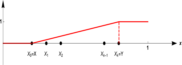
Figure 4: The graph of the function $u$ where the value $\min_{\left\{u\,|\,u(X)=0,u(Y)=1\right\}}\,{\cal E}(u)$ is reached.

Let us denote by $m$ the natural integer such that:

$$X\underset{m}{\sim}Y$$

One may introduce, the, for any integer $p$, the sequence of points $\left(X_{j}\right)_{0\leqslant j\leqslant 2^{p}}$ such that:

$$X_{0}=X\quad,\quad X_{2^{p}}=Y$$

and, for any integer $j$ such that $0<j<2^{p}-1$:

$$X_{j}\,\in\,V_{p+1}\quad,\quad X_{j}\underset{p+1}{\sim}X_{j+1}$$

In the case of the unit interval, the normalization constant is:

$$r^{-1}=\displaystyle\frac{1}{2}$$

One has then:

$$\begin{array}[]{ccc}{\cal{E}}(u,u)&=&\displaystyle\lim_{p\to+\infty}{\cal{E}}_{p}(u,u)\\ &=&\displaystyle\lim_{m\to+\infty}r^{-p}\,{\cal E}_{\Gamma_{{\cal W}_{p}}}(u)\\ &=&\displaystyle\lim_{p\to+\infty}\displaystyle\sum_{(X,Y)\,\in\,V_{p}^{2},\,X\underset{p}{\sim}Y}r^{-p}\,\left(u_{\mid V_{p}}(X)-u_{\mid V_{p}}(Y)\right)^{2}\\ &=&\displaystyle\lim_{p\to+\infty}\displaystyle\sum_{(X,Y)\,\in\,V_{p}^{2},\,X\underset{p}{\sim}Y}\displaystyle\frac{1}{2^{p}}\,\left(u_{\mid V_{p}}(X)-u_{\mid V_{p}}(Y)\right)^{2}\\ &=&\displaystyle\lim_{p\to+\infty}\displaystyle\sum_{j=0}^{k-1}\displaystyle\frac{1}{2^{p}}\,\left(u\left(X+\displaystyle\frac{j}{2^{p}}\right)-u\left(X+\displaystyle\frac{j+1}{2^{p}}\right)\right)^{2}\\ &=&\displaystyle\int_{X}^{Y}\displaystyle\frac{dt}{(Y-X)^{2}}\\ &=&\displaystyle\frac{1}{Y-X}\\ \end{array}$$

If $d_{{\mathbb{R}}}$ denotes the usual Euclidean distance on ${\mathbb{R}}$:

$$\forall\,(X,Y)\,\in{\mathbb{R}}^{2}\,:\quad d_{{\mathbb{R}}}(X,Y)=|Y-X|$$

one has then:

$$\begin{array}[]{ccc}\displaystyle\min_{\left\{u\,|\,u(X)=0,u(Y)=1\right\}}\,{\cal E}(u)&=&\displaystyle\frac{1}{d_{{\mathbb{R}}}(X,Y)}\end{array}$$

Let us now consider, more generally, a fractal domain $\cal F$, in an Euclidean space of dimension $d\,\in\,{\mathbb{N}}^{\star}$, equipped with the distance  $d_{{\mathbb{R}}^{d}}$. If, one has, in advance, defined an energy on $\cal F$, it is worth searching wether there exists a real number $\beta$ such that:

$$\forall\,(X,Y)\,\in\,{\cal F}^{2}\,:\quad\left(\min_{\left\{u\,|\,u(X)=0,u(Y)=1\right\}}\,{\cal E}(u)\right)^{-1}\sim\left(d_{{\mathbb{R}}^{d}}(X,Y)\right)^{\beta}$$

In the case of the Sierpiǹski gasket $\cal SG$ (we refer to [StrichartzFunctionalAnalysis]), Robert S. Strichartz lays the emphasis upon the fact that, given $X\underset{m}{\sim}Y$, one has:

$$\min_{\left\{u\,|\,u(X)=0,u(Y)=1\right\}}\,{\cal E}(u)\lesssim r_{\cal SG}^{m}=\left(\displaystyle\frac{3}{5}\right)^{m}$$

This also corresponds thus to the order of the diameter of the $m^{th}-$order cells.

Since the Sierpiǹski gasket $\cal SG$ is obtained from the initial triangle of diameter 1 by means of three contractions, the respective ratios of which are equal to $\displaystyle\frac{1}{2}$, one has simply to look the real number $\beta_{\cal SG}$ such that:

$$\left(\displaystyle\frac{1}{2}\right)^{m\,\beta_{\cal SG}}=\left(\displaystyle\frac{3}{5}\right)^{m}$$

This leads to:

$$\beta_{\cal SG}=\displaystyle\frac{\ln\frac{5}{3}}{\ln 2}$$

Definition 3.3.

Dimension of the graph $\Gamma_{\cal W}$, in the effective resistance metric

The dimension of the graph $\Gamma_{\cal W}$, in the effective resistance metric, is the strictly positive number $d_{Gamma_{\cal W}}$ such that, given a strictly positive real number $r$, and a point $X\,\in\,{\Gamma_{\cal W}}$, for the $X-$centered ball of radius $r$, denoted by ${\cal B}_{r}(X)$:

$$\mu\left({\cal B}_{r}(X)\right)=r^{d_{\Gamma_{\cal W}}}$$

Proposition 3.2.

The dimension of the graph $\Gamma_{\cal W}$, in the effective resistance metric, is given by:

1. First case: $\lambda>\displaystyle\frac{1}{N_{b}}$.
   

   $$d_{\Gamma_{\cal W}}=\displaystyle\frac{\ln\frac{N_{b}}{\lambda}}{(5-2\,D_{\cal W})\,\ln N_{b}}$$

2. Second case: $\lambda<\displaystyle\frac{1}{N_{b}}$.
   

   $$d_{\Gamma_{\cal W}}=\displaystyle\frac{2}{5-2\,D_{\cal W}}$$

Proof.

Remark 3.2.

Once again, it is worth having a look at the case of the Sierpiński gasket. Robert S. Strichartz stars from the fact that the measure of $m^{th}-$order cells is $\displaystyle\frac{1}{3^{m}}$. Two consecutive points $x$ and $y$ are such that, for the effective resistance metric

$$d(x,y)\sim\left(\displaystyle\frac{3}{5}\right)^{m}$$

For the self-similar measure $\mu_{\cal SG}$, which affects the value $\displaystyle\frac{1}{3^{m}}$ to each  $m^{th}-$order cell, one has simply to look for the real number $d_{\cal SG}$ such that:

$$\left(\displaystyle\frac{3}{5}\right)^{m\,d_{\cal SG}}=\displaystyle\frac{1}{3^{m}}$$

which leads to:

$$d_{\cal SG}=\displaystyle\frac{\ln 3}{\ln\frac{5}{3}}$$

One may then deduce from the above an estimate, for the effective resistance metric, of the measure of a $X-$centered ball of radius $r$, denoted by ${\cal B}_{r}(X)$:

$$\mu_{\cal SG}\left({\cal B}_{r}(x)\right)=r^{d_{\cal SG}}$$

Let us now go back to the graph $\Gamma_{\cal W}$.

Given a natural integer $m$, and two points $X$ and $Y$ such that $X\underset{m}{\sim}Y$:

$$\min_{\left\{u\,|\,u(X)=0,u(Y)=1\right\}}\,{\cal E}(u)\lesssim\eta_{2-D_{\cal W}}^{-2}\,r^{-m}=\eta_{2-D_{\cal W}}^{-2}\,N_{b}^{(5-2\,D_{\cal W})\,m}$$

For the detailed calculations which enable one to obtain the normalization constants, we refer to [27].

For the self-similar measure $\tilde{\mu}$ introduced in the above, each $m^{th}-$order cell, i.e. each simple polygon ${\cal P}_{m,j}$, $0\leqslant j\leqslant N_{b}^{m}-1$, with $N_{b}$ sides and $N_{b}$ vertices, has a measure of the order of:

$$(N_{b}-1)\,\displaystyle\frac{\eta^{m}}{N_{b}^{m}}$$

The points $X$ and $Y$ such that $X\underset{m}{\sim}Y$ belong to a $m^{th}-$order subcell, which is the intersection of a simple polygon ${\cal P}_{m,j}$, $0\leqslant j\leqslant N_{b}^{m}-1$, with the rectangle of which $X$ and $Y$ are two vertices, of width $\displaystyle\frac{\eta^{m}}{N_{b}^{m}}$, and height $\eta^{m}$. This subcell a has a measure, the order of which is thus:

$$\eta^{m}\,L_{m}=\displaystyle\frac{\eta^{m}}{(N_{b}-1)\,N_{b}^{m}}$$

1. First case: $\lambda>\displaystyle\frac{1}{N_{b}}$.
   

   One has simply to look for the real number $d_{\Gamma_{\cal W}}$ such that:

   $$\left(N_{b}^{5-2\,D_{\cal W}}\right)^{m\,d_{\Gamma_{\cal W}}}\quad\text{and}\quad\displaystyle\frac{\lambda^{m}}{N_{b}^{m}}$$

   are of the same order, which yields:

   $$d_{\Gamma_{\cal W}}=\displaystyle\frac{\ln\frac{N_{b}}{\lambda}}{(5-2\,D_{\cal W})\,\ln N_{b}}$$

2. Second case: $\lambda<\displaystyle\frac{1}{N_{b}}$.
   

   One has simply to look for the real number $d_{\Gamma_{\cal W}}$ such that:

   $$\left(N_{b}^{5-2\,D_{\cal W}}\right)^{m\,d_{\Gamma_{\cal W}}}\quad\text{and}\quad\displaystyle\frac{1}{N_{b}^{2m}}$$

   are of the same order, which yields:

   $$d_{\Gamma_{\cal W}}=\displaystyle\frac{2}{5-2\,D_{\cal W}}$$

∎

4 Detailed study of the spectrum of the Laplacian

As exposed by R. S. Strichartz in [29], one may bear in mind that the eigenvalues can be grouped into two categories:

1. initial eigenvalues, which a priori belong to the set of forbidden values (as for instance $\Lambda=2$) ;

2. continued eigenvalues, obtained by means of spectral decimation.

We present, in the sequel, a detailed study of the spectrum of $\Delta$, in the case where $N_{b}=3$, which can be easily extended to higher values of the integer $N_{b}$.

4.1 Eigenvalues and eigenvectors of $\Delta_{1}$

Let us recall that the vertices of the graph $\Gamma_{{\cal W}_{1}}$ are:

$$P_{0}\quad,\quad T_{0}\left(P_{1}\right)\quad,\quad T_{0}\left(P_{2}\right)\quad,\quad T_{1}\left(P_{0}\right)$$

$$P_{1}\quad,\quad T_{1}\left(P_{2}\right)\quad,\quad T_{2}\left(P_{0}\right)\quad,\quad T_{2}\left(P_{1}\right)\quad,\quad P_{2}$$

One may note that:

$$\text{Card}\,\left(V_{1}\setminus V_{0}\right)=4$$

Let us denote by $u$ an eigenfunction, for the eigenvalue $-\Lambda$. For the sake of simplicity, we set:

$$u\left(T_{0}\left(P_{1}\right)\right)=a\,\in\,{\mathbb{R}}\quad,\quad u\left(T_{0}\left(P_{2}\right)\right)=b\,\in\,{\mathbb{R}}\quad,\quad u\left(T_{2}\left(P_{0}\right)\right)=c\,\in\,{\mathbb{R}}\quad,\quad u\left(T_{2}\left(P_{1}\right)\right)=d\,\in\,{\mathbb{R}}$$

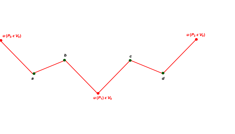
Figure 5: Successive values of an eigenfunction on $V_{1}$, in the case where $N_{b}=3$.

One has then:

$$\left\{\begin{array}[]{ccc}u(P_{0})-a+b-a&=&-\Lambda\,a\\ a-b+u(P_{1})-b&=&-\Lambda\,b\\ u(P_{1})-c+d-c&=&-\Lambda\,c\\ c-d+u(P_{2})-d&=&-\Lambda\,d\end{array}\right.$$

One may note that the only "Dirichlet eigenvalues", i.e. the ones related to the Dirichlet problem:

$$u_{|V_{0}}=0\quad\text{i.e.}\quad u(P_{0})=u(P_{1})=u(P_{2})=0$$

are obtained for:

$$\left\{\begin{array}[]{ccc}b&=&-(\Lambda-2)\,a\\ a&=&-(\Lambda-2)\,b\\ d&=&-(\Lambda-2)\,c\\ c&=&-(\Lambda-2)\,d\end{array}\right.$$

i.e.:

$$\left\{\begin{array}[]{ccc}b&=&(\Lambda-2)^{2}\,b\\ a&=&(\Lambda-2)^{2}\,a\\ d&=&(\Lambda-2)^{2}\,d\\ c&=&(\Lambda-2)^{2}\,c\end{array}\right.$$

The forbidden eigenvalue $\Lambda=2$ cannot thus be a Dirichlet one.

Let us consider the case where:

$$(\Lambda-2)^{2}=1$$

i.e.

$$\Lambda=1\quad\text{or}\quad\Lambda=3$$

The value $\Lambda=1$ leads to:

$$a=b\quad,\quad c=d$$

which yields a two-dimensional eigenspace. The multiplicity of the eigenvalue $\Lambda=1$ is 2.

For the eigenvalue $\Lambda=3$:

$$a=-b\quad,\quad c=-d$$

The eigenspace, for the eigenvalue $3$, has dimension 2. The multiplicity of the eigenvalue $\Lambda=3$ is 2.

Since the cardinal of $V_{1}\setminus V_{0}$ is:

$${\cal N}^{\cal S}_{1}-N_{b}=2\,N_{b}-2=4$$

one may note that we have the complete spectrum.

4.2 Eigenvalues of $\Delta_{2}$

Let us now look at the spectrum of $\Delta_{2}$. For the sake of simplicity, we will denote by $a$, $b$, $c$, $d$, $e$, $f$, $g$, $h$, the successive values of an eigenfunction at the $N_{b}^{2}-1$ points between $P_{0}$ and $P_{1}$, and by $a^{\prime}$, $b^{\prime}$, $c^{\prime}$, $d^{\prime}$, $e^{\prime}$, $f^{\prime}$, $g^{\prime}$, $h^{\prime}$, the successive values of an eigenfunction at the $N_{b}^{2}-1$ points between $P_{1}$ and $P_{2}$, as it appears on the following figure.

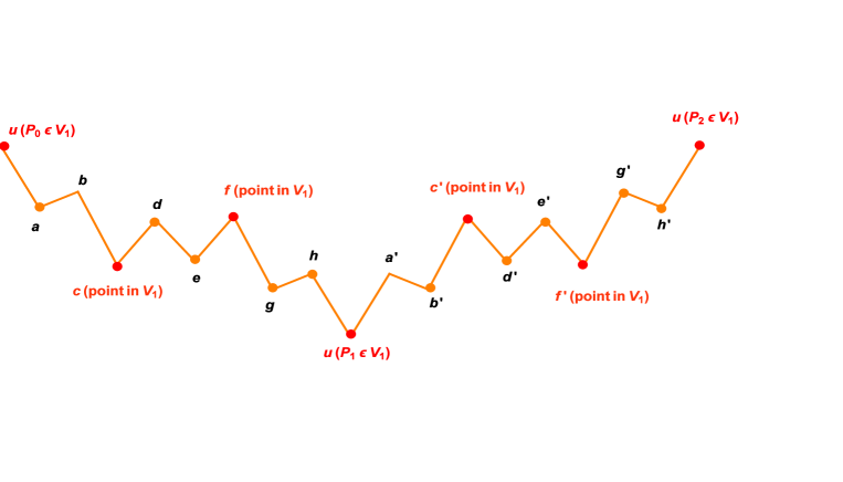
Figure 6: Successive values of an eigenfunction on $V_{2}$, in the case where $N_{b}=3$.

One has then:

$$\left\{\begin{array}[]{ccc}(2-\Lambda)\,a&=&-u(P_{0})-b\\ (2-\Lambda)\,b&=&-c-a\\ (2-\Lambda)\,c&=&-b-d\\ (2-\Lambda)\,d&=&-c-e\\ (2-\Lambda)\,e&=&-d-f\\ (2-\Lambda)\,f&=&-e-g\\ (2-\Lambda)\,g&=&-f-h\\ (2-\Lambda)\,h&=&-g-u(P_{1})\\ \end{array}\right.$$

and:

$$(2-\Lambda)\,u(P_{1})=-h-a^{\prime}$$

and:

$$\left\{\begin{array}[]{ccc}(2-\Lambda)\,a^{\prime}&=&-u(P_{1})-b^{\prime}\\ (2-\Lambda)\,b^{\prime}&=&-c^{\prime}-a^{\prime}\\ (2-\Lambda)\,c^{\prime}&=&-b^{\prime}-d^{\prime}\\ (2-\Lambda)\,d^{\prime}&=&-c^{\prime}-e^{\prime}\\ (2-\Lambda)\,e^{\prime}&=&-d^{\prime}-f^{\prime}\\ (2-\Lambda)\,f^{\prime}&=&-e^{\prime}-g^{\prime}\\ (2-\Lambda)\,g^{\prime}&=&-f^{\prime}-h^{\prime}\\ (2-\Lambda)\,h^{\prime}&=&-g^{\prime}-u(P_{2})\\ \end{array}\right.$$

One may note that the only Dirichlet eigenvalues, in the case where:

$$u_{|V_{0}}=0\quad\text{i.e.}\quad u(P_{0})=u(P_{1})=u(P_{2})=0$$

are obtained for:

$$\left\{\begin{array}[]{ccc}(2-\Lambda)\,a&=&-b\\ (2-\Lambda)\,b&=&-a\\ (2-\Lambda)\,c&=&-b-d\\ (2-\Lambda)\,d&=&-e\\ (2-\Lambda)\,e&=&-d\\ (2-\Lambda)\,f&=&-e-g\\ (2-\Lambda)\,g&=&-h\\ (2-\Lambda)\,h&=&-g\\ \end{array}\right.\quad\text{and}\quad 0=-h-a^{\prime}\quad\text{and}\quad\left\{\begin{array}[]{ccc}(2-\Lambda)\,a^{\prime}&=&-b^{\prime}\\ (2-\Lambda)\,b^{\prime}&=&-a^{\prime}\\ (2-\Lambda)\,c^{\prime}&=&-b^{\prime}-d^{\prime}\\ (2-\Lambda)\,d^{\prime}&=&-e^{\prime}\\ (2-\Lambda)\,e^{\prime}&=&-d^{\prime}\\ (2-\Lambda)\,f^{\prime}&=&-e^{\prime}-g^{\prime}\\ (2-\Lambda)\,g^{\prime}&=&-h^{\prime}\\ (2-\Lambda)\,h^{\prime}&=&-g^{\prime}\\ \end{array}\right.$$

i.e.:

$$\left\{\begin{array}[]{ccc}(2-\Lambda)\,a&=&-b\\ (2-\Lambda)^{2}\,b&=&b\\ \left\{1-(2-\Lambda)^{2}\right\}\,a&=&0\\ (2-\Lambda)\,c&=&-b-d\\ (2-\Lambda)\,d&=&-e\\ (2-\Lambda)^{2}\,e&=&e\\ (2-\Lambda)\,f&=&-e-g\\ (2-\Lambda)^{2}\,h&=&h\\ (2-\Lambda)\,h&=&-g\\ \end{array}\right.\quad\text{and}\quad 0=-h-a^{\prime}\quad\text{and}\quad\left\{\begin{array}[]{ccc}(2-\Lambda)\,a^{\prime}&=&-b^{\prime}\\ (2-\Lambda)^{2}\,b^{\prime}&=&b^{\prime}\\ \left\{1-(2-\Lambda)^{2}\right\}\,a^{\prime}&=&0\\ (2-\Lambda)\,c^{\prime}&=&-b^{\prime}-d^{\prime}\\ (2-\Lambda)\,d^{\prime}&=&-e^{\prime}\\ (2-\Lambda)^{2}\,e^{\prime}&=&e^{\prime}\\ (2-\Lambda)\,f^{\prime}&=&-e^{\prime}-g^{\prime}\\ (2-\Lambda)^{2}\,h^{\prime}&=&h^{\prime}\\ (2-\Lambda)\,h^{\prime}&=&-g^{\prime}\\ \end{array}\right.$$

The forbidden eigenvalue $\Lambda=2$ is not therefore a Dirichlet one.

Let us consider the case where:

$$(\Lambda-2)^{2}=1$$

i.e.

$$\Lambda=3\quad\text{or}\quad\Lambda=1$$

For $\Lambda=1$, one has:

$$\left\{\begin{array}[]{ccc}a&=&-b\\ c&=&-b-d\\ d&=&-e\\ f&=&-e-g\\ h&=&-g\\ \end{array}\right.\quad\text{and}\quad 0=-h-a^{\prime}\quad\text{and}\quad\left\{\begin{array}[]{ccc}a^{\prime}&=&-b^{\prime}\\ c^{\prime}&=&-b^{\prime}-d^{\prime}\\ d^{\prime}&=&-e^{\prime}\\ f^{\prime}&=&-e^{\prime}-g^{\prime}\\ h^{\prime}&=&-g^{\prime}\\ \end{array}\right.$$

The eigenspace, for $\Lambda=1$, has thus dimension 5. The multiplicity of the eigenvalue $\Lambda=1$ is 5.

For $\Lambda=3$:

$$\left\{\begin{array}[]{ccc}\left\{1-(2-\Lambda)^{2}\right\}\,a&=&0\\ c&=&b+d\\ d&=&e\\ f&=&e+g\\ h&=&g\\ \end{array}\right.\quad\text{and}\quad 0=-h-a^{\prime}\quad\text{and}\quad\left\{\begin{array}[]{ccc}a^{\prime}&=&b^{\prime}\\ c^{\prime}&=&b^{\prime}+d^{\prime}\\ d^{\prime}&=&e^{\prime}\\ f^{\prime}&=&e^{\prime}+g^{\prime}\\ h^{\prime}&=&g^{\prime}\\ \end{array}\right.$$

The eigenspace, for $\Lambda=3$, has thus dimension 5. The multiplicity of the eigenvalue $\Lambda=3$ is 5.

Let us now look at the continued eigenvalues, i.e. the ones obtained from the eigenvalues $\Lambda_{1}=1$ and $\Lambda_{1}=3$ by means of spectral decimation:

$$\Lambda_{2}=\phi^{-1}\left(\left(\phi\left(\Lambda_{1}\right)\right)^{\frac{1}{N_{b}}}\right)=\displaystyle\frac{\left\{\left(\phi\left(\Lambda_{1}\right)\right)^{\frac{1}{N_{b}}}+1\right\}^{2}}{\left(\phi\left(\Lambda_{1}\right)\right)^{\frac{1}{N_{b}}}}=\displaystyle\frac{\left\{\left(\displaystyle\frac{-2+\Lambda_{1}-\varepsilon\,\sqrt{\left\{\Lambda_{1}-2\right\}^{2}-4}}{2}\right)^{\frac{1}{N_{b}}}+1\right\}^{2}}{\left(\displaystyle\frac{-2+\Lambda_{1}-\varepsilon\,\sqrt{\left\{\Lambda_{1}-2\right\}^{2}-4}}{2}\right)^{\frac{1}{N_{b}}}}$$

where $\varepsilon\,\in\,\left\{-1,1\right\}$, for the values:

$$\Lambda_{1}\,\in\,\left\{1,3\right\}$$

As in [29], let us get rid, temporarily, of the Dirichlet conditions. We have thus:

$$\left\{\begin{array}[]{ccc}u(P_{0})+b&=&-(\Lambda-2)\,a\\ a+c&=&-(\Lambda-2)\,b\\ b+d&=&-(\Lambda-2)\,c\\ e+f&=&-\Lambda\,d\\ e+g&=&-(\Lambda-2)\,f\\ f+h&=&-(\Lambda-2)\,g\\ g+u(P_{1})&=&-(\Lambda-2)\,h\\ \end{array}\right.\quad\text{and}\quad(2-\Lambda)\,u(P_{1})=-h-a^{\prime}\quad\text{and}\quad\left\{\begin{array}[]{ccc}u(P_{1})+b^{\prime}&=&-(\Lambda-2)\,a^{\prime}\\ a^{\prime}+c^{\prime}&=&-(\Lambda-2)\,b^{\prime}\\ b^{\prime}+d^{\prime}&=&-(\Lambda-2)\,c^{\prime}\\ e^{\prime}+f^{\prime}&=&-\Lambda\,d^{\prime}\\ e^{\prime}+g^{\prime}&=&-(\Lambda-2)\,f^{\prime}\\ f^{\prime}+h^{\prime}&=&-(\Lambda-2)\,g^{\prime}\\ g^{\prime}+u(P_{2})&=&-(\Lambda-2)\,h^{\prime}\\ \end{array}\right.$$

For the initial eigenvalue $\Lambda_{1}=1$, it is worth noticing that the restriction of the associated eigenvalue $\Lambda$ to $V_{1}\setminus V_{0}$ must satisfy the eigensystem associated to the eigenvalue $\Lambda_{1}=1$, i.e.:

$$\left\{\begin{array}[]{ccc}u(P_{0})+f&=&-(\Lambda_{1}-2)\,c\\ u(P_{1})+c&=&-(\Lambda_{1}-2)\,f\\ \end{array}\right.\quad\text{and}\quad-(\Lambda-2)\,u(P_{1})=f+c^{\prime}\quad\text{and}\quad\left\{\begin{array}[]{ccc}u(P_{1})+f^{\prime}&=&-(\Lambda_{1}-2)\,c^{\prime}\\ u(P_{2})+c^{\prime}&=&-(\Lambda_{1}-2)\,f^{\prime}\\ \end{array}\right.$$

or:

$$\left\{\begin{array}[]{ccc}u(P_{0})+f&=&c\\ u(P_{1})+c&=&f\\ \end{array}\right.\quad\text{and}\quad-(\Lambda-2)\,u(P_{1})=f+c^{\prime}\quad\text{and}\quad\left\{\begin{array}[]{ccc}u(P_{1})+f^{\prime}&=&c^{\prime}\\ u(P_{2})+c^{\prime}&=&f^{\prime}\\ \end{array}\right.$$

i.e.:

$$u(P_{0})+u(P_{1})=0\quad\text{and}\quad u(P_{1})+u(P_{2})=0$$

For $u(P_{0})=u(P_{1})=u(P_{2})=0$, it works, and the Dirichlet conditions appear to be satisfied. One has then:

$$\left\{\begin{array}[]{ccc}b&=&-(\Lambda-2)\,a\\ c&=&\left\{-1+(\Lambda-2)^{2}\right\}\,a\\ d&=&(\Lambda-2)\,\left\{1-\left\{1-(\Lambda-2)^{2}\right\}\right\}\,a\\ e+f&=&-\Lambda\,(\Lambda-2)\,\left\{1-\left\{1-(\Lambda-2)^{2}\right\}\right\}\,a\\ e&=&(\Lambda-2)\,\,\left\{1-\left\{-1+(\Lambda-2)^{2}\right\}\right\}\,h\\ f&=&\left\{-1+(\Lambda-2)^{2}\right\}\,h\\ g&=&-(\Lambda-2)\,h\\ \end{array}\right.\quad,\quad c^{\prime}=-f\quad,\quad\left\{\begin{array}[]{ccc}b^{\prime}&=&-(\Lambda-2)\,a^{\prime}\\ c^{\prime}&=&\left\{-1+(\Lambda-2)^{2}\right\}\,a^{\prime}\\ d^{\prime}&=&(\Lambda-2)\,\left\{1-\left\{1-(\Lambda-2)^{2}\right\}\right\}\,a^{\prime}\\ e^{\prime}+f^{\prime}&=&-\Lambda\,(\Lambda-2)\,\left\{1-\left\{1-(\Lambda-2)^{2}\right\}\right\}\,a^{\prime}\\ e^{\prime}&=&(\Lambda-2)\,\,\left\{1-\left\{-1+(\Lambda-2)^{2}\right\}\right\}\,h^{\prime}\\ f^{\prime}&=&\left\{-1+(\Lambda-2)^{2}\right\}\,h^{\prime}\\ g^{\prime}&=&-(\Lambda-2)\,h^{\prime}\\ \end{array}\right.$$

We obtain thus an eigenspace, the dimension of which is $1$.

For the eigenvalue $\Lambda_{1}=1$, the spectral decimation spectral leads to:

$$\left(\displaystyle\frac{2-\Lambda_{2}+\varepsilon_{2}\,\rho\left(\omega_{2}\right)^{2}\,e^{i\,\theta\omega_{2}}}{2}\right)^{N_{b}}=\displaystyle\frac{1+\varepsilon_{1}\,\sqrt{3}\,e^{\frac{i\,\pi}{2}}}{2}$$

which leads to the quadruple eigenvalue:

$$\Lambda_{2}=2+\cos\displaystyle\frac{\pi}{9}+\sqrt{3}\,\sin\displaystyle\frac{\pi}{9}$$

For the eigenvalue $\Lambda_{1}=3$, the spectral decimation leads to the quadruple eigenvalue:

$$\Lambda_{2}=2\,\left\{1+\cos\displaystyle\frac{\pi}{9}\right\}$$

Since the cardinal of $V_{2}\setminus V_{0}$ is:

$${\cal N}^{\cal S}_{2}-{\cal N}^{\cal S}_{0}=16$$

one may note that we have the complete spectrum.

4.3 Eigenvalues of $\Delta_{3}$

As previously, one can easily check that the forbidden eigenvalue $\Lambda=2$ is not therefore a Dirichlet one.

One can also check that $\Lambda_{3}=1$ and $\Lambda_{3}=3$ are eigenvalues of $\Delta_{3}$, both with multiplicity 8.

From:

$$\Lambda_{\hookrightarrow 2,}=2\,\left\{1+\cos\displaystyle\frac{\pi}{9}\right\}$$

the spectral decimation leads then to the quadruple eigenvalue:

$$\Lambda_{\hookrightarrow 3}=4\,\cos^{2}\displaystyle\frac{\pi}{27}$$

From:

$$\Lambda_{\hookrightarrow 2}=2+\cos\displaystyle\frac{\pi}{9}+\sqrt{3}\,\sin\displaystyle\frac{\pi}{9}$$

the spectral decimation leads then to the quadruple eigenvalue:

$$\Lambda_{\hookrightarrow 3}=4\,\cos^{2}\displaystyle\frac{\pi}{54}$$

4.4 Eigenvalues of $\Delta_{m}$, $m\,\in\,{\mathbb{N}}$, $m\geqslant 4$

As previously, one can easily check that the forbidden eigenvalue $\Lambda=2$ is not therefore a Dirichlet one.

One can also check that $\Lambda_{m}=1$ and $\Lambda_{m}=3$ are eigenvalues of $\Delta_{m}$, both with multiplicity 2.

By induction, one may note that, due to the spectral decimation, the initial eigenvalue $\Lambda_{1}=1$ gives birth, at this $m^{th}$ step, to an eigenvalue $\Lambda_{m}$, of multiplicity $2^{m-1}$. In the same way, the initial eigenvalue $\Lambda_{1}=3$ gives birth, at this $m^{th}$ step, to an eigenvalue $\Lambda_{m}$, of multiplicity $2^{m-1}$.

Results are summarized in the following array:

$$\begin{array}[]{|c|c|c|c|c|r|}\hline\cr\\ \text{Initial eigenvalue}\,\Lambda_{1}&\text{continued eigenvalue}\,\Lambda_{2}&\text{continued eigenvalue $\Lambda_{\hookrightarrow 3}$}&\text{continued eigenvalue $\Lambda_{\hookrightarrow 4}$}\\ \hline\cr\\ 1&2+\cos\displaystyle\frac{\pi}{9}+\sqrt{3}\,\sin\displaystyle\frac{\pi}{9}&4\,\cos^{2}\displaystyle\frac{\pi}{27}&4\,\cos^{2}\displaystyle\frac{\pi}{81}\\ \hline\cr\\ 3&2\,\left\{1+\cos\displaystyle\frac{\pi}{9}\right\}&4\,\cos^{2}\displaystyle\frac{\pi}{54}&2\,\left\{1+\cos\displaystyle\frac{\pi}{81}\right\}\\ \hline\cr\end{array}$$

Property 4.1.

Let us introduce:

$$\Lambda=\displaystyle\lim_{m\to+\infty}\eta_{2-D_{\cal W}}^{-2}\,N_{b}^{(5-2\,D_{\cal W})\,m}$$

One may note that, due to the definition of the Laplacian $\Delta$, the limit exists.

4.5 Eigenvalue counting function

Definition 4.1.

Eigenvalue counting function

Let us introduce the eigenvalue counting function, related to $\Gamma_{\cal W}\setminus V_{0}$, such that, for any positive number $x$:

$${\cal N}^{\Gamma_{\cal W}\setminus V_{0}}(x)=\text{Card}\,\left\{\Lambda\,\text{Dirichlet eigenvalue of~{}$-\Delta$}\,:\quad\Lambda\leqslant x\right\}$$

Property 4.2.

Given a strictly positive integer, the cardinal of $V_{m}\setminus V_{0}$ is:

$${\cal N}^{\cal S}_{m}-{\cal N}^{\cal S}_{0}=2\,N_{b}^{m}-2$$

Let us denote by $\Lambda_{m}^{s}$ the largest eigenvalue, which is such that:

$$\eta_{2-D_{\cal W}}\,N_{b}^{m}\times 3\leqslant\Lambda_{m}^{s}\leqslant\eta_{2-D_{\cal W}}\,N_{b}^{m}\times 4$$

This leads to:

$${\cal N}^{\Gamma_{\cal W}}(C\,N_{b}^{m})=2\,N_{b}^{m}-2\quad,\quad 3\leqslant C\leqslant 4$$

If one looks for an asymptotic growth rate of the form

$${\cal N}^{\Gamma_{\cal W}}(x)\sim x^{\alpha}$$

one obtains:

$$\alpha=1$$

By following [29], one may note that the ratio

$$\frac{{\cal N}^{\Gamma_{\cal W}}(x)}{x}$$

is bounded above and away from zero, and admits a limit along any sequence of the form $C\,N_{b}^{m}$, $C>0$, $m\,\in\,{\mathbb{N}}^{\star}$. This enables one to deduce the existence of a periodic function $g$, the period of which is equal to $\ln N_{b}$, discontinuous at the value $3$, such that:

$$\lim_{x\to+\infty}\left\{\displaystyle\frac{{\cal N}^{\Gamma_{\cal W}}(x)}{x}-g(\ln x)\right\}=0$$

$$\begin{array}[]{|c|c|c| }\hline\cr\\ \text{Level}&\text{Cardinal of the Dirichlet spectrum, in the case where~{}$N_{b}=3$}\\ \hline\cr\\ m&2\,N_{b}^{m}-2\\ \hline\cr\\ 1&4\\ \hline\cr\\ 2&16\\ \hline\cr\\ 3&52\\ \hline\cr\\ 4&160\\ \hline\cr\end{array}$$

Figure 7: The graph of the function $m\mapsto\displaystyle\frac{ln{{\cal N}^{\Gamma_{\cal W}}(C\,N_{b}^{m})}}{m}$ in the case where $\lambda=\displaystyle\frac{1}{2}$, and $N_{b}=3$.

Remark 4.1.

Existing results of J. Kigami and M. Lapidus [10], and also of R. S. Strichartz [29], yield:

$${\cal N}^{\Gamma_{\cal W}}(x)=G(x)\,x^{\alpha_{\Gamma_{\cal W}}}+{\cal O}(1)$$

with:

$$\alpha_{\Gamma_{\cal W}}=\displaystyle\frac{d_{\Gamma_{\cal W}}}{d_{\Gamma_{\cal W}}+1}=\displaystyle\frac{\ln\frac{N_{b}}{\lambda}}{\ln\frac{N_{b}}{\lambda}+(5-2\,D_{\cal W})\,\ln N_{b}}$$

where:

$$d_{\Gamma_{\cal W}}=\displaystyle\frac{\ln\frac{N_{b}}{\lambda}}{(5-2\,D_{\cal W})\,\ln N_{b}}$$

is the dimension of the graph $\Gamma_{\cal W}$ for the resistance metric.

Thanks

The author would like to thank R. Str., who suggested for our previous work, the introduction of specific energies to fully take into account the very specific geometry of the problem.

References

- [1] J. Kigami, A harmonic calculus on the Sierpiński spaces, Japan J. Appl. Math., 8 (1989), pages 259-290.
- [2] J. Kigami, Harmonic calculus on p.c.f. self-similar sets, Trans. Amer. Math. Soc., 335(1993), pages 721-755.
- [3] R. S. Strichartz, Analysis on fractals, Notices of the AMS, 46(8), 1999, pages 1199-1208.
- [4] J. Kigami, R. S. Strichartz, K. C. Walker, Constructing a Laplacian on the Diamond Fractal, A. K. Peters, Ltd, Experimental Mathematics, 10(3), pages 437-448.
- [5] Cl. David, Laplacian, on the graph of the Weierstrass function, arXiv:1703.03371v1.
- [6] J. Kaplan, J. Mallet-Paret and J. Yorke, The Lyapunov dimension of a nowhere differentiable attracting torus, Ergodic Theory Dynam. Systems 4, 1984, pages 261–281.
- [7] T.-Y. Hu, K.-S. Lau, Fractal Dimensions and Singularities of the Weierstrass Type Functions, Transactions of the American Mathematical Society, 1993, 335(2), pages 649-665.
- [8] Weixiao Shen, Hausdorff dimension of the graphs of the classical Weierstrass functions, arXiv:1505.03986.
- [9] G. Keller, A simpler proof for the dimension of the graph of the classical Weierstrass function, Ann. Inst. Poincaré, 53(1), 2017, pages 169-181.
- [10] J. Kigami and M. Lapidus, Weyl’s problem for the spectral distribution of Laplacians on P.C.F. self-similar fractalss, Communications in Mathematical Physics, 204, 2003, pages 399-444.
- [11] K. Weierstrass, Über continuirliche Funktionen eines reellen Arguments, die für keinen Werth des letzteren einen bestimmten Differentialquotienten besitzen, 1967, in Karl Weiertrass Mathematische Werke, Abhandlungen II, Johnson, Gelesen in der Königl. Akademie der Wissenchaften am 18 Juli 1872, 2, pages 71-74.
- [12] E. C. Titschmarsh, The theory of functions, Second edition, Oxford University Press, 1939, pages 351-353.
- [13] G. H. Hardy, Theorems Connected with Maclaurin’s Test for the Convergence of Series, Proc. London Math. Soc., 1911, s2-9 (1), pages 126-144.
- [14] A. S. Besicovitch, H. D. Ursell, Sets of Fractional Dimensions, Journal of the London Mathematical Society, 12 (1), 1937, pages 18-25.
- [15] B. B. Mandelbrot, Fractals: form, chance, and dimension, San Francisco: Freeman, 1977.
- [16] K. Falconer, The Geometry of Fractal Sets, 1985, Cambridge University Press, pages 114-149.
- [17] B. Hunt, The Hausdorff dimension of graphs of Weierstrass functions, Proc. Amer. Math. Soc., 126 (3), 1998, pages 791-800.
- [18] K. Barańsky, B. Bárány, J. Romanowska, On the dimension of the graph of the classical Weierstrass function, Advances in Math., 265, 2014, pages 32-59.
- [19] G. Keller, A simpler proof for the dimension of the graph of the classical Weierstrass function, Ann. Inst. Poincaré, 53(1), 2017, pages 169-181.
- [20] M. F. Barnsley, S. Demko, Iterated Function Systems and the Global Construction of Fractals, The Proceedings of the Royal Society of London, A(399), 1985, pages 243-275.
- [21] M.V. Berry, and Z. V. Lewis, On the Weierstrass-Mandelbrot function, Proc. R. Soc. Lond., A(370), 1980, pages 459-484.
- [22] C. Sabot, Existence and uniqueness of diffusions on finitely ramified self-similar fractals, Annales scientifiques de l’É.N.S. 4 e série, 30(4), 1997, pages 605-673.
- [23] A. Beurling, J. Deny, Espaces de Dirichlet. I. Le cas élémentaire, Acta Mathematica, 99 (1), 1985, pages 203-224.
- [24] M. Fukushima, Y. Oshima, and M. Takeda, Dirichlet forms and symmetric Markov processes, 1994, Walter de Gruyter & Co.
- [25] J. Kigami, Harmonic Analysis for Resistance Forms, Journal of Functional Analysis, 204, 2003, pages 399-444.
- [26] N. Riane, 2016, Autour du Laplacien sur des domaines présentant un caractère fractal, Mémoire de recherche, M2 Mathématiques de la modélisation, Université Pierre et Marie Curie-Paris 6.
- [27] Cl. David et N. Riane, Formes de Dirichlet et fonctions harmoniques sur le graphe de la fonction de Weierstrass, preprint, HAL.
- [28] R. S. Strichartz, Function spaces on fractals, Journal of Functional Analysis, 198(1), 2003, pages 43-83.
- [29] R. S. Strichartz, Differential Equations on Fractals, A tutorial, Princeton University Press, 2006.
- [30] J. E. Hutchinson, Fractals and self similarity, Indiana University Mathematics Journal 30, 1981, pages 713-747.
- [31] R. S. Strichartz, A. Taylor and T. Zhang, Densities of Self-Similar Measures on the Line, Experimental Mathematics, 4(2), 1995, pages 101-128.
- [32] M. Fukushima and T. Shima, On a spectral analysis for the Sierpinski gasket, Potential Anal., 1, 1992, pages 1-3.