Cosmological Analysis of Scalar Field Models in f​(R,T)𝑓𝑅𝑇f(R,T) Gravity

M. Sharif and Iqra Nawazish
Department of Mathematics, University of the Punjab,
Quaid-e-Azam Campus, Lahore-54590, Pakistan
msharif.math@pu.edu.pkiqranawazish07@gmail.com
Abstract

This paper determines the existence of Noether symmetry in non-minimally coupled f​(R,T)𝑓𝑅𝑇f(R,T) gravity admitting minimal coupling with scalar field models. We consider a generalized spacetime which corresponds to different anisotropic and homogeneous universe models. We formulate symmetry generators along with conserved quantities through Noether symmetry technique for direct and indirect curvature-matter coupling. For dust and perfect fluids, we evaluate exact solutions and construct their cosmological analysis through some cosmological parameters. We conclude that decelerated expansion is obtained for quintessence model with dust distribution while perfect fluid with dominating potential energy over kinetic energy leads to current cosmic expansion for both phantom as well as quintessence models.

Keywords: Noether symmetry; Conserved quantity; f​(R,T)𝑓𝑅𝑇f(R,T) gravity.
PACS: 04.20.Jb; 04.50.Kd; 95.36.+x.

1 Introduction

The generic function in f​(R)𝑓𝑅f(R) gravity is a coupling-free function which helps to resolve many cosmological issues. Nojiri and Odintsov [1] proposed the concept of non-minimal curvature-matter coupling which introduced a fresh insight among researchers. This coupling successfully incorporates clusters of galaxies or dark matter in galaxies, yielding natural preheating conditions corresponding to inflationary models as well as introduces the idea of traversable wormholes in the absence of any exotic matter [2]. Harko et al. [3] proposed a new version of modified theory whose generic function incorporates curvature as well as matter known as f​(R,T)𝑓𝑅𝑇f(R,T) gravity (T𝑇T is the trace of energy-momentum tensor). This function induces strong interactions of gravity and matter which play a dynamical role to analyze current cosmic expansion [4]. Sharif and Zubair [5] investigated some cosmic issues like energy conditions, thermodynamics, anisotropic exact solutions, reconstruction of some dark energy models and also studied stability issue in this gravity.

The curiosity for exact solutions of higher order non-linear differential equations keep motivating the researchers as these are extensively used to investigate different cosmic aspects. Harko and Lake [6] discussed exact solutions of cylindrical spacetime in the presence of non-minimal coupling between R𝑅R and matter Lagrangian density (β„’msubscriptβ„’π‘š\mathcal{L}_{m}). The higher order non-linear differential equations of f​(R,T)𝑓𝑅𝑇f(R,T) gravity attract many researchers to construct cosmological analysis via exact solutions of the field equations. Sharif and Zubair [7] considered exponential and power-law expansions to evaluate some exact solutions and kinematical quantities of Bianchi type I (BI) model in this gravity. Shamir and Raza [8] formulated exact solutions corresponding to cosmic string as well as non-null electromagnetic field. Shamir [9] found exact solutions of locally rotationally symmetric BI model and studied their physical behavior through cosmological parameters.

In mathematical physics and theoretical cosmology, continuous symmetry reduces the complexity of non-linear system which successfully yields exact solutions. In a dynamical system, Noether symmetry proposes a correspondence between infinitesimal symmetry generator and conserved quantity. Capozziello et al. [10] used this approach to find exact solutions of spherically symmetric spacetime in f​(R)𝑓𝑅f(R) gravity. Hussain et al. [11] investigated the existence of Noether symmetry of power-law f​(R)𝑓𝑅f(R) model and found boundary term to be vanished for flat FRW universe model but Shamir et al. [12] obtained non-zero boundary term of the same model. Momeni et al. [13] explored Noether point symmetry of isotropic universe in mimetic f​(R)𝑓𝑅f(R) and f​(R,T)𝑓𝑅𝑇f(R,T) gravity theories. Shamir and Ahmad [14] constructed exact solutions in f​(𝒒,T)𝑓𝒒𝑇f(\mathcal{G},T) gravity (𝒒𝒒\mathcal{G} denotes Gauss-Bonnet term).

Sanyal [15] determined exact solutions of Kantowski-Sachs (KS) universe model through Noether symmetry technique in non-minimally coupled gravity with scalar field. Camci and Kucukakca [16] extended this work by adding BI as well as BIII universe models and formulated explicit forms of scalar field. Kucukakca et al. [17] discussed the presence of Noether symmetry to formulate exact solutions of locally rotationally symmetric BI universe. Camci et al. [18] generalized this work for anisotropic universe models such as BI, BIII and KS. We have obtained exact solutions of f​(R)𝑓𝑅f(R) power-law model [19] as well as f​(R,T)𝑓𝑅𝑇f(R,T) model admitting indirect non-minimal curvature-matter coupling [20].

In non-minimally coupled gravitational theory, the Noether symmetry approach is extensively used to study different cosmological models and the dynamical role of various scalar field models [21]. Vakili [22] identified the existence of Noether point symmetry along with conserved quantity for flat FRW universe and studied the behavior of effective equation of state (EoS) parameter for quintessence model in f​(R)𝑓𝑅f(R) gravity. Zhang et al. [23] explored multiple scalar field scenario and formulated a relationship of potential function with quintessence and phantom models. Jamil et al. [24] ensured the presence of Noether symmetry with conservation law for f​(R)𝑓𝑅f(R) tachyon model. Sharif and Shafique [25] obtained exact solutions of isotropic and anisotropic universe models in scalar-tensor theory non-minimally coupled with torsion scalar.

In this paper, we discuss the existence of Noether symmetries of non-minimally coupled f​(R,T)𝑓𝑅𝑇f(R,T) gravity interacting with generalized scalar field model. The format of the paper is as follows. Section 2 introduces some basic aspects of this gravity. In section 3, we discuss all possible Noether symmetries with associated conserved quantities for two particular models of this theory. We also formulate exact solutions for dust as well as perfect fluid distribution and study their physical behavior through some cosmological parameters. In the last section, we present final remarks.

2 Some Basics of f​(R,T)𝑓𝑅𝑇f(R,T) Gravity

We consider the action incorporating gravity, matter and scalar field as

ℐ=∫d4​xβ€‹βˆ’g​[β„’g+β„’m+β„’Ο•],ℐsuperscript𝑑4π‘₯𝑔delimited-[]subscriptℒ𝑔subscriptβ„’π‘šsubscriptβ„’italic-Ο•\mathcal{I}=\int d^{4}x\sqrt{-g}[\mathcal{L}_{g}+\mathcal{L}_{m}+\mathcal{L}_{\phi}], (1)

where g𝑔g denotes determinant of the metric tensor, β„’gsubscriptℒ𝑔\mathcal{L}_{g} and β„’Ο•subscriptβ„’italic-Ο•\mathcal{L}_{\phi} represent gravity and scalar field Lagrangian densities. For non-minimal coupling, the gravitational Lagrangian is considered to be a generic function f​(R,T)𝑓𝑅𝑇f(R,T) admitting minimal coupling only with β„’msubscriptβ„’π‘š\mathcal{L}_{m} and β„’Ο•subscriptβ„’italic-Ο•\mathcal{L}_{\phi} [3]. In this case, the metric variation of β„’gsubscriptℒ𝑔\mathcal{L}_{g} and β„’msubscriptβ„’π‘š\mathcal{L}_{m} yields

fR​(R,T)​RΞΌβ€‹Ξ½βˆ’12​f​(R,T)​gμ​ν+(gΞΌβ€‹Ξ½β€‹βˆ‡ΞΌβˆ‡ΞΌβˆ’βˆ‡ΞΌβˆ‡Ξ½)​fR​(R,T)+fT​(R,T)​Tμ​νsubscript𝑓𝑅𝑅𝑇subscriptπ‘…πœ‡πœˆ12𝑓𝑅𝑇subscriptπ‘”πœ‡πœˆsubscriptπ‘”πœ‡πœˆsubscriptβˆ‡πœ‡superscriptβˆ‡πœ‡subscriptβˆ‡πœ‡subscriptβˆ‡πœˆsubscript𝑓𝑅𝑅𝑇subscript𝑓𝑇𝑅𝑇subscriptπ‘‡πœ‡πœˆ\displaystyle f_{R}(R,T)R_{\mu\nu}-\frac{1}{2}f(R,T)g_{\mu\nu}+(g_{\mu\nu}\nabla_{\mu}\nabla^{\mu}-\nabla_{\mu}\nabla_{\nu})f_{R}(R,T)+f_{T}(R,T)T_{\mu\nu}
+fT​(R,T)​(gμ​ν​ℒmβˆ’2​TΞΌβ€‹Ξ½βˆ’2​gΞΌβ€‹Ξ½β€‹βˆ‚2β„’mβˆ‚gΞΌβ€‹Ξ½β€‹βˆ‚gμ​ν)=ΞΊ2​Tμ​ν,subscript𝑓𝑇𝑅𝑇subscriptπ‘”πœ‡πœˆsubscriptβ„’π‘š2subscriptπ‘‡πœ‡πœˆ2superscriptπ‘”πœ‡πœˆsuperscript2subscriptβ„’π‘šsuperscriptπ‘”πœ‡πœˆsuperscriptπ‘”πœ‡πœˆsuperscriptπœ…2subscriptπ‘‡πœ‡πœˆ\displaystyle+f_{T}(R,T)(g_{\mu\nu}\mathcal{L}_{m}-2T_{\mu\nu}-2g^{\mu\nu}\frac{\partial^{2}\mathcal{L}_{m}}{\partial g^{\mu\nu}\partial g^{\mu\nu}})=\kappa^{2}T_{\mu\nu},

where subscripts R𝑅R and T𝑇T describe corresponding partial derivatives of f𝑓f, βˆ‡ΞΌsubscriptβˆ‡πœ‡\nabla_{\mu} indicates covariant derivative and Tμ​νsubscriptπ‘‡πœ‡πœˆT_{\mu\nu} represents energy-momentum tensor. The divergence of energy-momentum tensor leads to

βˆ‡ΞΌTμ​ν=fTΞΊ2βˆ’fT​[(Tμ​ν+Ξ˜ΞΌβ€‹Ξ½)β€‹βˆ‡ΞΌln⁑fT+βˆ‡ΞΌΞ˜ΞΌβ€‹Ξ½βˆ’gΞΌβ€‹Ξ½β€‹βˆ‡ΞΌT2].superscriptβˆ‡πœ‡subscriptπ‘‡πœ‡πœˆsubscript𝑓𝑇superscriptπœ…2subscript𝑓𝑇delimited-[]subscriptπ‘‡πœ‡πœˆsubscriptΞ˜πœ‡πœˆsuperscriptβˆ‡πœ‡subscript𝑓𝑇superscriptβˆ‡πœ‡subscriptΞ˜πœ‡πœˆsubscriptπ‘”πœ‡πœˆsuperscriptβˆ‡πœ‡π‘‡2\nabla^{\mu}T_{\mu\nu}=\frac{f_{T}}{\kappa^{2}-f_{T}}\left[(T_{\mu\nu}+\Theta_{\mu\nu})\nabla^{\mu}\ln f_{T}+\nabla^{\mu}\Theta_{\mu\nu}-\frac{g_{\mu\nu}\nabla^{\mu}T}{2}\right].

In non-minimally coupled modified gravity, the energy-momentum tensor remains no more conserved. This non-zero divergence introduces an extra force in equation of motion which is responsible for deviation of massive test particles from geodesic trajectories.

A generalization of some anisotropic and homogeneous universe models is given as [26]

d​s2=βˆ’d​t2+a2​(t)​d​r2+b2​(t)​(d​θ2+΢​(ΞΈ)​d​ϕ2),𝑑superscript𝑠2𝑑superscript𝑑2superscriptπ‘Ž2𝑑𝑑superscriptπ‘Ÿ2superscript𝑏2𝑑𝑑superscriptπœƒ2πœπœƒπ‘‘superscriptitalic-Ο•2ds^{2}=-dt^{2}+a^{2}(t)dr^{2}+b^{2}(t)(d\theta^{2}+\zeta(\theta)d\phi^{2}), (2)

where aπ‘Ža and b𝑏b are scale factors and ΢​(ΞΈ)=ΞΈ,sin⁑h​θ,sinβ‘ΞΈπœπœƒπœƒβ„Žπœƒπœƒ\zeta(\theta)={\theta,~{}\sin h\theta,~{}\sin\theta} identify BI, BIII and KS models with the following relationship

1΢​d2​΢d​θ2=βˆ’ΞΎ.1𝜁superscript𝑑2πœπ‘‘superscriptπœƒ2πœ‰\frac{1}{\zeta}\frac{d^{2}\zeta}{d\theta^{2}}=-\xi.

For ΞΎ=0,βˆ’1,1πœ‰011\xi=0,-1,1, the spacetime (2) corresponds to BI, BIII and KS universe models, respectively. For perfect fluid, the energy-momentum tensor is

Tμ​ν=(ρm+pm)​uμ​uΞ½+pm​gμ​ν,subscriptπ‘‡πœ‡πœˆsubscriptπœŒπ‘šsubscriptπ‘π‘šsubscriptπ‘’πœ‡subscriptπ‘’πœˆsubscriptπ‘π‘šsubscriptπ‘”πœ‡πœˆT_{\mu\nu}=(\rho_{m}+p_{m})u_{\mu}u_{\nu}+p_{m}g_{\mu\nu},

where pmsubscriptπ‘π‘šp_{m} and ρmsubscriptπœŒπ‘š\rho_{m} define pressure and energy density, respectively whereas u𝑒u represents four-velocity of the fluid. For the action (1), the Lagrangian density of matter and scalar fields are defined as [27]

β„’m=pm​(a,b),β„’Ο•=Ο΅2​gΞΌβ€‹Ξ½β€‹βˆ‚ΞΌΟ•β€‹βˆ‚Ξ½Ο•βˆ’V​(Ο•),formulae-sequencesubscriptβ„’π‘šsubscriptπ‘π‘šπ‘Žπ‘subscriptβ„’italic-Ο•italic-Ο΅2superscriptπ‘”πœ‡πœˆsubscriptπœ‡italic-Ο•subscript𝜈italic-ϕ𝑉italic-Ο•\mathcal{L}_{m}=p_{m}(a,b),\quad\mathcal{L}_{\phi}=\frac{\epsilon}{2}g^{\mu\nu}\partial_{\mu}\phi\partial_{\nu}\phi-V(\phi), (3)

where V​(Ο•)𝑉italic-Ο•V(\phi) denotes potential energy of the scalar field and Ο΅=1,βˆ’1italic-Ο΅11\epsilon=1,-1 indicate scalar field models, i.e., quintessence and phantom models.

Phantom model suffers with number of troubles like violation of dominant energy condition, the entropy of phantom-dominated universe is negative and consequently, black holes disappear. Such a universe ends up with a finite time future singularity dubbed as big-rip singularity [28]. Different ideas are proposed to cure the troubles of this singularity such as considering phantom acceleration as transient phenomenon with different scalar potentials or to modify the gravity, couple dark energy with dark matter or to use particular forms of EoS for dark energy taking into account some quantum effects (giving rise to the second quantum gravity era) which may delay/stop the singularity occurrence [29]. Inserting Eq.(3) into (1), we obtain

ℐ=∫d4​xβ€‹βˆ’g​[f​(R,T)2​κ2+pm​(a,b)+Ο΅2​gΞΌβ€‹Ξ½β€‹βˆ‚ΞΌΟ•β€‹βˆ‚Ξ½Ο•βˆ’V​(Ο•)],ℐsuperscript𝑑4π‘₯𝑔delimited-[]𝑓𝑅𝑇2superscriptπœ…2subscriptπ‘π‘šπ‘Žπ‘italic-Ο΅2superscriptπ‘”πœ‡πœˆsubscriptπœ‡italic-Ο•subscript𝜈italic-ϕ𝑉italic-Ο•\mathcal{I}=\int d^{4}x\sqrt{-g}[\frac{f(R,T)}{2\kappa^{2}}+p_{m}(a,b)+\frac{\epsilon}{2}g^{\mu\nu}\partial_{\mu}\phi\partial_{\nu}\phi-V(\phi)], (4)

where

R=2a​b2​(a¨​b2+2​a​b​bΒ¨+2​b​a˙​bΛ™+a​b2Λ™+a​ξ),T=3​pm​(a,b)βˆ’Οm​(a,b).formulae-sequence𝑅2π‘Žsuperscript𝑏2Β¨π‘Žsuperscript𝑏22π‘Žπ‘Β¨π‘2π‘Λ™π‘ŽΛ™π‘π‘ŽΛ™superscript𝑏2π‘Žπœ‰π‘‡3subscriptπ‘π‘šπ‘Žπ‘subscriptπœŒπ‘šπ‘Žπ‘\displaystyle R=\frac{2}{ab^{2}}\left(\ddot{a}b^{2}+2ab\ddot{b}+2b\dot{a}\dot{b}+a\dot{b^{2}}+a\xi\right),\quad T=3p_{m}(a,b)-\rho_{m}(a,b).

To evaluate Lagrangian corresponding to the action (4) for configuration space 𝒬={a,b,R,T,Ο•}π’¬π‘Žπ‘π‘…π‘‡italic-Ο•\mathcal{Q}=\{a,b,R,T,\phi\}, we use Lagrange multiplier approach which yields

β„’β„’\displaystyle\mathcal{L} =\displaystyle= ab2[f(R,T)βˆ’RfR(R,T)+fT(R,T)(3pm(a,b)βˆ’Οm(a,b)βˆ’T)βˆ’Ο΅β€‹Ο•Λ™22\displaystyle ab^{2}[f(R,T)-Rf_{R}(R,T)+f_{T}(R,T)(3p_{m}(a,b)-\rho_{m}(a,b)-T)-\frac{\epsilon\dot{\phi}^{2}}{2} (5)
+\displaystyle+ pm(a,b)βˆ’V(Ο•)]βˆ’(4baΛ™bΛ™+2abΛ™2βˆ’2aΞΎ)fR(R,T)βˆ’(2b2aΛ™RΛ™+4abbΛ™RΛ™)\displaystyle p_{m}(a,b)-V(\phi)]-(4b\dot{a}\dot{b}+2a\dot{b}^{2}-2a\xi)f_{R}(R,T)-(2b^{2}\dot{a}\dot{R}+4ab\dot{b}\dot{R})
Γ—\displaystyle\times fR​R​(R,T)βˆ’(2​b2​a˙​TΛ™+4​a​b​b˙​TΛ™)​fR​T​(R,T).subscript𝑓𝑅𝑅𝑅𝑇2superscript𝑏2Λ™π‘ŽΛ™π‘‡4π‘Žπ‘Λ™π‘Λ™π‘‡subscript𝑓𝑅𝑇𝑅𝑇\displaystyle f_{RR}(R,T)-(2b^{2}\dot{a}\dot{T}+4ab\dot{b}\dot{T})f_{RT}(R,T).

In a dynamical system, the Euler-Lagrange equation, Hamiltonian (β„‹β„‹\mathcal{H}) and conjugate momenta (pisubscript𝑝𝑖p_{i}) play a significant role to determine basic features of the system, defined as

βˆ‚β„’βˆ‚qiβˆ’d​pid​t=0,β„‹=βˆ‘iqΛ™i​piβˆ’β„’,pi=βˆ‚β„’βˆ‚qΛ™i,formulae-sequenceβ„’superscriptπ‘žπ‘–π‘‘subscript𝑝𝑖𝑑𝑑0formulae-sequenceβ„‹subscript𝑖superscriptΛ™π‘žπ‘–subscript𝑝𝑖ℒsubscript𝑝𝑖ℒsuperscriptΛ™π‘žπ‘–\displaystyle\frac{\partial\mathcal{L}}{\partial q^{i}}-\frac{dp_{i}}{dt}=0,\quad\mathcal{H}=\sum_{i}\dot{q}^{i}p_{i}-\mathcal{L},\quad p_{i}=\frac{\partial\mathcal{L}}{\partial\dot{q}^{i}},

where qisuperscriptπ‘žπ‘–q^{i} shows n𝑛n coordinates of the system. For Lagrangian (5), the conjugate momenta take the following form

pasubscriptπ‘π‘Ž\displaystyle p_{a} =\displaystyle= βˆ’4​b​b˙​fRβˆ’2​b2​(R˙​fR​R+T˙​fR​T),pΟ•=βˆ’a​b2​ϡ​ϕ˙,4𝑏˙𝑏subscript𝑓𝑅2superscript𝑏2˙𝑅subscript𝑓𝑅𝑅˙𝑇subscript𝑓𝑅𝑇subscript𝑝italic-Ο•π‘Žsuperscript𝑏2italic-Ο΅Λ™italic-Ο•\displaystyle-4b\dot{b}f_{R}-2b^{2}(\dot{R}f_{RR}+\dot{T}f_{RT}),\quad p_{\phi}=-ab^{2}\epsilon\dot{\phi},
pbsubscript𝑝𝑏\displaystyle p_{b} =\displaystyle= βˆ’4​fR​(a​bΛ™+b​aΛ™)βˆ’4​a​b​(R˙​fR​R+T˙​fR​T),4subscriptπ‘“π‘…π‘ŽΛ™π‘π‘Λ™π‘Ž4π‘Žπ‘Λ™π‘…subscript𝑓𝑅𝑅˙𝑇subscript𝑓𝑅𝑇\displaystyle-4f_{R}(a\dot{b}+b\dot{a})-4ab(\dot{R}f_{RR}+\dot{T}f_{RT}),
pRsubscript𝑝𝑅\displaystyle p_{R} =\displaystyle= βˆ’(4​a​b​bΛ™+2​b2​aΛ™)​fR​R,pT=βˆ’(4​a​b​bΛ™+2​b2​aΛ™)​fR​T.4π‘Žπ‘Λ™π‘2superscript𝑏2Λ™π‘Žsubscript𝑓𝑅𝑅subscript𝑝𝑇4π‘Žπ‘Λ™π‘2superscript𝑏2Λ™π‘Žsubscript𝑓𝑅𝑇\displaystyle-(4ab\dot{b}+2b^{2}\dot{a})f_{RR},\quad p_{T}=-(4ab\dot{b}+2b^{2}\dot{a})f_{RT}.

The dynamical equations of the system are

2​fR​(R,T)​(b2Λ™b2+2​bΒ¨b+2​ξb2)+fβˆ’R​fR+fT​(3​pm​(a,b)βˆ’Οm​(a,b)βˆ’T)2subscript𝑓𝑅𝑅𝑇˙superscript𝑏2superscript𝑏22¨𝑏𝑏2πœ‰superscript𝑏2𝑓𝑅subscript𝑓𝑅subscript𝑓𝑇3subscriptπ‘π‘šπ‘Žπ‘subscriptπœŒπ‘šπ‘Žπ‘π‘‡\displaystyle 2f_{R}(R,T)\left(\frac{\dot{b^{2}}}{b^{2}}+\frac{2\ddot{b}}{b}+\frac{2\xi}{b^{2}}\right)+f-Rf_{R}+f_{T}(3p_{m}(a,b)-\rho_{m}(a,b)-T) (8)
+\displaystyle+ pm(a,b)βˆ’Ο΅β€‹Ο•Λ™22βˆ’V(Ο•)+a{fT(3pm,aβˆ’Οm,a)+pm,a}+4bβˆ’1bΛ™RΛ™fR​R\displaystyle p_{m}(a,b)-\frac{\epsilon\dot{\phi}^{2}}{2}-V(\phi)+a\{f_{T}(3p_{m},_{{}_{a}}-\rho_{m},_{{}_{a}})+p_{m},_{{}_{a}}\}+4b^{-1}\dot{b}\dot{R}f_{RR}
+\displaystyle+ 4​bβˆ’1​b˙​T˙​fR​T+2​R¨​fR​R+2​RΛ™2​fR​R​R+4​R˙​T˙​fR​R​T+2​T¨​fR​T+2​TΛ™2​fR​T​T=0,4superscript𝑏1˙𝑏˙𝑇subscript𝑓𝑅𝑇2¨𝑅subscript𝑓𝑅𝑅2superscript˙𝑅2subscript𝑓𝑅𝑅𝑅4˙𝑅˙𝑇subscript𝑓𝑅𝑅𝑇2¨𝑇subscript𝑓𝑅𝑇2superscript˙𝑇2subscript𝑓𝑅𝑇𝑇0\displaystyle 4b^{-1}\dot{b}\dot{T}f_{RT}+2\ddot{R}f_{RR}+2\dot{R}^{2}f_{RRR}+4\dot{R}\dot{T}f_{RRT}+2\ddot{T}f_{RT}+2\dot{T}^{2}f_{RTT}=0,
2​fR​(aΒ¨a+a˙​bΛ™a​b+bΒ¨b)+fβˆ’R​fR+fT​(3​pm​(a,b)βˆ’Οm​(a,b)βˆ’T)+pm​(a,b)2subscriptπ‘“π‘…Β¨π‘Žπ‘ŽΛ™π‘ŽΛ™π‘π‘Žπ‘Β¨π‘π‘π‘“π‘…subscript𝑓𝑅subscript𝑓𝑇3subscriptπ‘π‘šπ‘Žπ‘subscriptπœŒπ‘šπ‘Žπ‘π‘‡subscriptπ‘π‘šπ‘Žπ‘\displaystyle 2f_{R}\left(\frac{\ddot{a}}{a}+\frac{\dot{a}\dot{b}}{ab}+\frac{\ddot{b}}{b}\right)+f-Rf_{R}+f_{T}(3p_{m}(a,b)-\rho_{m}(a,b)-T)+p_{m}(a,b)
βˆ’\displaystyle- ϡ​ϕ˙22βˆ’V(Ο•)+b2{fT(3pm,bβˆ’Οm,b))+pm,b}+2(aβˆ’1aΛ™RΛ™+RΒ¨)fR​R+2RΛ™2\displaystyle\frac{\epsilon\dot{\phi}^{2}}{2}-V(\phi)+\frac{b}{2}\{f_{T}(3p_{m},_{{}_{b}}-\rho_{m},_{{}_{b}}))+p_{m},_{{}_{b}}\}+2(a^{-1}\dot{a}\dot{R}+\ddot{R})f_{RR}+2\dot{R}^{2}
Γ—\displaystyle\times fR​R​R+2​(aβˆ’1​a˙​TΛ™+TΒ¨)​fR​T+2​(bβˆ’1​b˙​RΛ™+2​R˙​TΛ™+TΛ™2)​fR​R​T+2​bβˆ’1​b˙​T˙​fR​T​T=0,subscript𝑓𝑅𝑅𝑅2superscriptπ‘Ž1Λ™π‘ŽΛ™π‘‡Β¨π‘‡subscript𝑓𝑅𝑇2superscript𝑏1˙𝑏˙𝑅2˙𝑅˙𝑇superscript˙𝑇2subscript𝑓𝑅𝑅𝑇2superscript𝑏1˙𝑏˙𝑇subscript𝑓𝑅𝑇𝑇0\displaystyle f_{RRR}+2(a^{-1}\dot{a}\dot{T}+\ddot{T})f_{RT}+2(b^{-1}\dot{b}\dot{R}+2\dot{R}\dot{T}+\dot{T}^{2})f_{RRT}+2b^{-1}\dot{b}\dot{T}f_{RTT}=0,
fR​T​(3​pm​(a,b)βˆ’Οm​(a,b)βˆ’T)=0,fT​T​(3​pm​(a,b)βˆ’Οm​(a,b)βˆ’T)=0,formulae-sequencesubscript𝑓𝑅𝑇3subscriptπ‘π‘šπ‘Žπ‘subscriptπœŒπ‘šπ‘Žπ‘π‘‡0subscript𝑓𝑇𝑇3subscriptπ‘π‘šπ‘Žπ‘subscriptπœŒπ‘šπ‘Žπ‘π‘‡0\displaystyle f_{RT}(3p_{m}(a,b)-\rho_{m}(a,b)-T)=0,\quad f_{TT}(3p_{m}(a,b)-\rho_{m}(a,b)-T)=0,
ϡ​ϕ¨+2​ϡ​bβˆ’1​b˙​ϕ˙+ϡ​aβˆ’1​aΛ™β€‹Ο•Λ™βˆ’V′​(Ο•)=0.italic-ϡ¨italic-Ο•2italic-Ο΅superscript𝑏1˙𝑏˙italic-Ο•italic-Ο΅superscriptπ‘Ž1Λ™π‘ŽΛ™italic-Ο•superscript𝑉′italic-Ο•0\displaystyle\epsilon\ddot{\phi}+2\epsilon b^{-1}\dot{b}\dot{\phi}+\epsilon a^{-1}\dot{a}\dot{\phi}-V^{\prime}(\phi)=0.

In order to evaluate total energy of the dynamical system, we formulate Hamiltonian as

β„‹β„‹\displaystyle\mathcal{H} =\displaystyle= 2​fR​(b2Λ™b2+2​a˙​bΛ™a​b)+2​(2​bΛ™b+aΛ™a)​R˙​fR​R+2​(2​bΛ™b+aΛ™a)​T˙​fR​T+fβˆ’R​fR2subscript𝑓𝑅˙superscript𝑏2superscript𝑏22Λ™π‘ŽΛ™π‘π‘Žπ‘22Λ™π‘π‘Λ™π‘Žπ‘ŽΛ™π‘…subscript𝑓𝑅𝑅22Λ™π‘π‘Λ™π‘Žπ‘ŽΛ™π‘‡subscript𝑓𝑅𝑇𝑓𝑅subscript𝑓𝑅\displaystyle 2f_{R}\left(\frac{\dot{b^{2}}}{b^{2}}+\frac{2\dot{a}\dot{b}}{ab}\right)+2\left(\frac{2\dot{b}}{b}+\frac{\dot{a}}{a}\right)\dot{R}f_{RR}+2\left(\frac{2\dot{b}}{b}+\frac{\dot{a}}{a}\right)\dot{T}f_{RT}+f-Rf_{R} (9)
+\displaystyle+ fT​(3​pm​(a,b)βˆ’Οm​(a,b)βˆ’T)+pm​(a,b)+ϡ​ϕ˙22βˆ’V​(Ο•)+2​ξ​fRb2.subscript𝑓𝑇3subscriptπ‘π‘šπ‘Žπ‘subscriptπœŒπ‘šπ‘Žπ‘π‘‡subscriptπ‘π‘šπ‘Žπ‘italic-Ο΅superscriptΛ™italic-Ο•22𝑉italic-Ο•2πœ‰subscript𝑓𝑅superscript𝑏2\displaystyle f_{T}(3p_{m}(a,b)-\rho_{m}(a,b)-T)+p_{m}(a,b)+\frac{\epsilon\dot{\phi}^{2}}{2}-V(\phi)+\frac{2\xi f_{R}}{b^{2}}.

The Hamiltonian constraint β„‹=0β„‹0\mathcal{H}=0 yields total pressure of the dynamical system.

3 Noether Symmetry and Conserved Quantities

The Noether symmetry approach helps to solve complicated non-linear system of partial differential equations yielding exact solutions at theoretical grounds of physics and cosmology. Noether theorem states that if Lagrangian of a dynamical system remains invariant under a continuous group then group generator leads to the associated conserved quantity. The conservation of energy and linear momentum appears for translational invariant Lagrangian in time and position, respectively whereas the angular momentum is conserved for rotationally symmetric Lagrangian [30]. In gravitational theories, the presence of conserved quantities also enhances physical interpretation of theory but if it does not appreciate the existence of any conserved quantity, then the theory will be abandoned due to its non-physical features.

To investigate the existence of Noether symmetry and associated conserved quantity in non-minimally coupled gravitational theory, we consider the first order prolongation K[1]superscript𝐾delimited-[]1K^{[1]} of continuous group defined as

K[1]=K+(Ο†j,t+Ο†j,iqΛ™iβˆ’Ο‘,tqΛ™jβˆ’Ο‘,iqΛ™iqΛ™j)βˆ‚βˆ‚qΛ™j,\displaystyle K^{[1]}=K+(\varphi^{j},_{t}+\varphi^{j},_{i}\dot{q}^{i}-\vartheta,_{t}\dot{q}^{j}-\vartheta,_{i}\dot{q}^{i}\dot{q}^{j})\frac{\partial}{\partial\dot{q}^{j}}, (10)

where cosmic time t𝑑t is considered to be an affine parameter and K𝐾K represents symmetry generator given by

K𝐾\displaystyle K =\displaystyle= ϑ​(t,qi)β€‹βˆ‚βˆ‚t+Ο†j​(t,qi)β€‹βˆ‚βˆ‚qj.italic-ϑ𝑑superscriptπ‘žπ‘–π‘‘superscriptπœ‘π‘—π‘‘superscriptπ‘žπ‘–superscriptπ‘žπ‘—\displaystyle\vartheta(t,q^{i})\frac{\partial}{\partial t}+\varphi^{j}(t,q^{i})\frac{\partial}{\partial q^{j}}. (11)

Here Ο‘italic-Ο‘\vartheta and Ο†jsuperscriptπœ‘π‘—\varphi^{j} are unknown coefficients of the generator. The existence of Noether symmetry is ensured when K𝐾K follows the invariance condition as

K[1]​ℒ+(D​ϑ)​ℒ=D​B​(t,qi),D=βˆ‚βˆ‚t+qΛ™iβ€‹βˆ‚βˆ‚qi,formulae-sequencesuperscript𝐾delimited-[]1ℒ𝐷italic-ϑℒ𝐷𝐡𝑑superscriptπ‘žπ‘–π·π‘‘superscriptΛ™π‘žπ‘–superscriptπ‘žπ‘–K^{[1]}\mathcal{L}+(D\vartheta)\mathcal{L}=DB(t,q^{i}),\quad D=\frac{\partial}{\partial t}+\dot{q}^{i}\frac{\partial}{\partial q^{i}}, (12)

where D𝐷D is the total derivative while B𝐡B represents boundary term of K𝐾K. When the symmetry generator becomes independent of affine parameter then boundary term along with first order prolongation vanishes yielding

K=Ο±i​(qi)β€‹βˆ‚βˆ‚qi+[dd​t​(Ο±i​(qi))]β€‹βˆ‚βˆ‚qΛ™i,LK​ℒ=0,formulae-sequence𝐾superscriptitalic-ϱ𝑖superscriptπ‘žπ‘–superscriptπ‘žπ‘–delimited-[]𝑑𝑑𝑑superscriptitalic-ϱ𝑖superscriptπ‘žπ‘–superscriptΛ™π‘žπ‘–subscript𝐿𝐾ℒ0K=\varrho^{i}(q^{i})\frac{\partial}{\partial q^{i}}+\left[\frac{d}{dt}(\varrho^{i}(q^{i}))\right]\frac{\partial}{\partial\dot{q}^{i}},\quad L_{K}\mathcal{L}=0, (13)

where L𝐿L identifies Lie derivative. The symmetries coming from symmetry generators (11) and (13) lead to corresponding conservation law through the first integral defined as

Ξ£=Bβˆ’Ο‘β€‹β„’βˆ’(Ο†jβˆ’qΛ™j​ϑ)β€‹βˆ‚β„’βˆ‚qΛ™j,Ξ£=βˆ’Ξ·jβ€‹βˆ‚β„’βˆ‚qΛ™j.formulae-sequenceΣ𝐡italic-Ο‘β„’superscriptπœ‘π‘—superscriptΛ™π‘žπ‘—italic-Ο‘β„’superscriptΛ™π‘žπ‘—Ξ£superscriptπœ‚π‘—β„’superscriptΛ™π‘žπ‘—\Sigma=B-\vartheta\mathcal{L}-(\varphi^{j}-\dot{q}^{j}\vartheta)\frac{\partial\mathcal{L}}{\partial\dot{q}^{j}},\quad\Sigma=-\eta^{j}\frac{\partial\mathcal{L}}{\partial\dot{q}^{j}}. (14)

For Q={t,a,b,R,T,Ο•}π‘„π‘‘π‘Žπ‘π‘…π‘‡italic-Ο•Q=\{t,a,b,R,T,\phi\}, the infinitesimal symmetry generator and corresponding first order prolongation take the form

K𝐾\displaystyle K =\displaystyle= Ο„β€‹βˆ‚βˆ‚t+Ξ±β€‹βˆ‚βˆ‚a+Ξ²β€‹βˆ‚βˆ‚b+Ξ³β€‹βˆ‚βˆ‚R+Ξ΄β€‹βˆ‚βˆ‚T+Ξ·β€‹βˆ‚βˆ‚Ο•,K[1]=Ο„β€‹βˆ‚βˆ‚t+Ξ±β€‹βˆ‚βˆ‚a+Ξ²β€‹βˆ‚βˆ‚bπœπ‘‘π›Όπ‘Žπ›½π‘π›Ύπ‘…π›Ώπ‘‡πœ‚italic-Ο•superscript𝐾delimited-[]1πœπ‘‘π›Όπ‘Žπ›½π‘\displaystyle\tau\frac{\partial}{\partial t}+\alpha\frac{\partial}{\partial a}+\beta\frac{\partial}{\partial b}+\gamma\frac{\partial}{\partial R}+\delta\frac{\partial}{\partial T}+\eta\frac{\partial}{\partial\phi},\quad K^{[1]}=\tau\frac{\partial}{\partial t}+\alpha\frac{\partial}{\partial a}+\beta\frac{\partial}{\partial b} (15)
+\displaystyle+ Ξ³β€‹βˆ‚βˆ‚R+Ξ΄β€‹βˆ‚βˆ‚T+Ξ±Λ™β€‹βˆ‚βˆ‚aΛ™+Ξ²Λ™β€‹βˆ‚βˆ‚bΛ™+Ξ³Λ™β€‹βˆ‚βˆ‚RΛ™+Ξ΄Λ™β€‹βˆ‚βˆ‚TΛ™+Ξ·Λ™β€‹βˆ‚βˆ‚Ο•Λ™,π›Ύπ‘…π›Ώπ‘‡Λ™π›ΌΛ™π‘ŽΛ™π›½Λ™π‘Λ™π›ΎΛ™π‘…Λ™π›ΏΛ™π‘‡Λ™πœ‚Λ™italic-Ο•\displaystyle\gamma\frac{\partial}{\partial R}+\delta\frac{\partial}{\partial T}+\dot{\alpha}\frac{\partial}{\partial\dot{a}}+\dot{\beta}\frac{\partial}{\partial\dot{b}}+\dot{\gamma}\frac{\partial}{\partial\dot{R}}+\dot{\delta}\frac{\partial}{\partial\dot{T}}+\dot{\eta}\frac{\partial}{\partial\dot{\phi}},

where time derivative of unknown coefficients Ο„,Ξ±,Ξ²,Ξ³,Ξ΄πœπ›Όπ›½π›Ύπ›Ώ\tau,~{}\alpha,~{}\beta,~{}\gamma,~{}\delta and Ξ·πœ‚\eta are

ΟƒΛ™lsubscriptΛ™πœŽπ‘™\displaystyle\dot{\sigma}_{{}_{l}} =\displaystyle= D​σlβˆ’qΛ™i​D​τ,l=1​…​5,𝐷subscriptπœŽπ‘™superscriptΛ™π‘žπ‘–π·πœπ‘™1…5\displaystyle D\sigma_{{}_{l}}-\dot{q}^{i}D\tau,\quad l=1...5, (16)

Here Οƒ1,Οƒ2,Οƒ3,Οƒ4subscript𝜎1subscript𝜎2subscript𝜎3subscript𝜎4\sigma_{1},~{}\sigma_{2},~{}\sigma_{3},~{}\sigma_{4} and Οƒ5subscript𝜎5\sigma_{5} correspond to Ξ±,Ξ²,Ξ³,δ𝛼𝛽𝛾𝛿\alpha,~{}\beta,~{}\gamma,~{}\delta and Ξ·πœ‚\eta, respectively.

In order to discuss the presence of Noether symmetry generator and relative conserved quantity of the model (2), we insert the first order prolongation (10) alongwith (11) in (12), it follows a system of equations given in Appendix A. From Eq.(A7), we have either fR,fR​R,fR​T=0subscript𝑓𝑅subscript𝑓𝑅𝑅subscript𝑓𝑅𝑇0f_{R},~{}f_{RR},~{}f_{RT}=0 with Ο„,a,Ο„,b,Ο„,R,Ο„,Tβ‰ 0\tau,_{{}_{a}},~{}\tau,_{{}_{b}},~{}\tau,_{{}_{R}},~{}\tau,_{{}_{T}}\neq 0 or vice versa. For non-trivial solution, we consider second possibility (Ο„,a,Ο„,b,Ο„,R,Ο„,T=0\tau,_{{}_{a}},~{}\tau,_{{}_{b}},~{}\tau,_{{}_{R}},~{}\tau,_{{}_{T}}=0) as the first choice yields trivial solution. We investigate the existence of symmetry generators, relative conserved quantities for the following two models [3]

  • β€’

    f​(R,T)𝑓𝑅𝑇f(R,T)=R+2​g​(T)𝑅2𝑔𝑇R+2g(T),

  • β€’

    f​(R,T)𝑓𝑅𝑇f(R,T)=F​(R)+h​(R)​g​(T)πΉπ‘…β„Žπ‘…π‘”π‘‡F(R)+h(R)g(T).

We also formulate corresponding exact solutions to analyze cosmological picture of these two models.

3.1 f​(R,T)=R+2​g​(T)𝑓𝑅𝑇𝑅2𝑔𝑇f(R,T)=R+2g(T)

This model incorporates an indirect non-minimal curvature-matter coupling and also admits a correspondence with standard cosmological constant cold dark matter (ΛΛ\LambdaCDM) model if it comprises a trace dependent cosmological constant defined as

f​(R,T)=R+2​Λ​(T)+g​(T).𝑓𝑅𝑇𝑅2Λ𝑇𝑔𝑇f(R,T)=R+2\Lambda(T)+g(T). (17)

To evaluate the coefficients of symmetry generator (11), we solve the system (A1)-(A22) via separation of variables method which gives

α𝛼\displaystyle\alpha =\displaystyle= Ξ±1​(t)​α2​(a)​α3​(b)​α4​(R)​α5​(T)​α6​(Ο•),Ξ΄=Ξ΄1​(t)​δ2​(a)​δ3​(b)​δ4​(R)​δ5​(T)​δ6​(Ο•),subscript𝛼1𝑑subscript𝛼2π‘Žsubscript𝛼3𝑏subscript𝛼4𝑅subscript𝛼5𝑇subscript𝛼6italic-ϕ𝛿subscript𝛿1𝑑subscript𝛿2π‘Žsubscript𝛿3𝑏subscript𝛿4𝑅subscript𝛿5𝑇subscript𝛿6italic-Ο•\displaystyle\alpha_{1}(t)\alpha_{2}(a)\alpha_{3}(b)\alpha_{4}(R)\alpha_{5}(T)\alpha_{6}(\phi),\quad\delta=\delta_{1}(t)\delta_{2}(a)\delta_{3}(b)\delta_{4}(R)\delta_{5}(T)\delta_{6}(\phi),
γ𝛾\displaystyle\gamma =\displaystyle= Ξ³1​(t)​γ2​(a)​γ3​(b)​γ4​(R)​γ5​(T)​γ6​(Ο•),Ξ·=Ξ·1​(t)​η2​(a)​η3​(b)​η4​(R)​η5​(T)​η6​(Ο•),subscript𝛾1𝑑subscript𝛾2π‘Žsubscript𝛾3𝑏subscript𝛾4𝑅subscript𝛾5𝑇subscript𝛾6italic-Ο•πœ‚subscriptπœ‚1𝑑subscriptπœ‚2π‘Žsubscriptπœ‚3𝑏subscriptπœ‚4𝑅subscriptπœ‚5𝑇subscriptπœ‚6italic-Ο•\displaystyle\gamma_{1}(t)\gamma_{2}(a)\gamma_{3}(b)\gamma_{4}(R)\gamma_{5}(T)\gamma_{6}(\phi),\quad\eta=\eta_{1}(t)\eta_{2}(a)\eta_{3}(b)\eta_{4}(R)\eta_{5}(T)\eta_{6}(\phi),
β𝛽\displaystyle\beta =\displaystyle= Ξ²1​(t)​β2​(a)​β3​(b)​β4​(R)​β5​(T)​β6​(Ο•),Ο„=Ο„1​(t),subscript𝛽1𝑑subscript𝛽2π‘Žsubscript𝛽3𝑏subscript𝛽4𝑅subscript𝛽5𝑇subscript𝛽6italic-Ο•πœsubscript𝜏1𝑑\displaystyle\beta_{1}(t)\beta_{2}(a)\beta_{3}(b)\beta_{4}(R)\beta_{5}(T)\beta_{6}(\phi),\quad\tau=\tau_{1}(t),
B𝐡\displaystyle B =\displaystyle= B1​(t)​B2​(a)​B3​(b)​B4​(R)​B5​(T)​B6​(Ο•).subscript𝐡1𝑑subscript𝐡2π‘Žsubscript𝐡3𝑏subscript𝐡4𝑅subscript𝐡5𝑇subscript𝐡6italic-Ο•\displaystyle B_{1}(t)B_{2}(a)B_{3}(b)B_{4}(R)B_{5}(T)B_{6}(\phi).

For these coefficients, the system (A1)-(A22) yields

α𝛼\displaystyle\alpha =\displaystyle= βˆ’2​a​c1,Ξ²=c1​b,Ξ³=0,Ξ΄=0,Ξ·=c4,formulae-sequence2π‘Žsubscript𝑐1𝛽subscript𝑐1𝑏formulae-sequence𝛾0formulae-sequence𝛿0πœ‚subscript𝑐4\displaystyle-2ac_{{}_{1}},\quad\beta=c_{{}_{1}}b,\quad\gamma=0,\quad\delta=0,\quad\eta=c_{{}_{4}},
B𝐡\displaystyle B =\displaystyle= c2​t+c3,Ο„=c5,V​(Ο•)=c6​ϕ+c7,formulae-sequencesubscript𝑐2𝑑subscript𝑐3𝜏subscript𝑐5𝑉italic-Ο•subscript𝑐6italic-Ο•subscript𝑐7\displaystyle c_{{}_{2}}t+c_{{}_{3}},\quad\tau=c_{{}_{5}},\quad V(\phi)=c_{{}_{6}}\phi+c_{{}_{7}},
pm​(a,b)subscriptπ‘π‘šπ‘Žπ‘\displaystyle p_{m}(a,b) =\displaystyle= βˆ’c4​c6​ln⁑a+2​c1​a12​b2​c1βˆ’2​ξb2βˆ’c2​ln⁑a2​c1​a​b2,subscript𝑐4subscript𝑐6π‘Ž2subscript𝑐1superscriptπ‘Ž12𝑏2subscript𝑐12πœ‰superscript𝑏2subscript𝑐2π‘Ž2subscript𝑐1π‘Žsuperscript𝑏2\displaystyle-\frac{c_{{}_{4}}c_{{}_{6}}\ln a+2c_{{}_{1}}a^{\frac{1}{2}}b}{2c_{{}_{1}}}-\frac{2\xi}{b^{2}}-\frac{c_{{}_{2}}\ln a}{2c_{{}_{1}}ab^{2}}, (18)
ρm​(a,b)subscriptπœŒπ‘šπ‘Žπ‘\displaystyle\rho_{m}(a,b) =\displaystyle= βˆ’3​c4​c6​ln⁑a+2​c1​a12​b2​c1βˆ’6​ξb2βˆ’3​c2​ln⁑a2​c1​a​b2,3subscript𝑐4subscript𝑐6π‘Ž2subscript𝑐1superscriptπ‘Ž12𝑏2subscript𝑐16πœ‰superscript𝑏23subscript𝑐2π‘Ž2subscript𝑐1π‘Žsuperscript𝑏2\displaystyle-\frac{3c_{{}_{4}}c_{{}_{6}}\ln a+2c_{{}_{1}}a^{\frac{1}{2}}b}{2c_{{}_{1}}}-\frac{6\xi}{b^{2}}-\frac{3c_{{}_{2}}\ln a}{2c_{{}_{1}}ab^{2}}, (19)

where cisubscript𝑐𝑖c_{i}’s (i=1​…​7)𝑖1…7(i=1...7) denotes arbitrary constants. For these coefficients, we split the symmetry generator and corresponding first integral into the following form

K1subscript𝐾1\displaystyle K_{1} =\displaystyle= βˆ‚βˆ‚t,Ξ£1=βˆ’a​b2​{fβˆ’R​fR+fT​(3​pmβˆ’Οmβˆ’T)+pmβˆ’c6β€‹Ο•βˆ’c7}𝑑subscriptΞ£1π‘Žsuperscript𝑏2𝑓𝑅subscript𝑓𝑅subscript𝑓𝑇3subscriptπ‘π‘šsubscriptπœŒπ‘šπ‘‡subscriptπ‘π‘šsubscript𝑐6italic-Ο•subscript𝑐7\displaystyle\frac{\partial}{\partial t},\quad\Sigma_{1}=-ab^{2}\{f-Rf_{R}+f_{T}(3p_{m}-\rho_{m}-T)+p_{m}-c_{{}_{6}}\phi-c_{{}_{7}}\}
+\displaystyle+ 2​a​ξ​fRβˆ’4​b​a˙​b˙​fRβˆ’2​a​bΛ™2​fRβˆ’Ο΅β€‹Ο•Λ™2​a​b22,2π‘Žπœ‰subscript𝑓𝑅4π‘Λ™π‘ŽΛ™π‘subscript𝑓𝑅2π‘Žsuperscript˙𝑏2subscript𝑓𝑅italic-Ο΅superscriptΛ™italic-Ο•2π‘Žsuperscript𝑏22\displaystyle 2a\xi f_{R}-4b\dot{a}\dot{b}f_{R}-2a\dot{b}^{2}f_{R}-\frac{\epsilon\dot{\phi}^{2}ab^{2}}{2},
K2subscript𝐾2\displaystyle K_{2} =\displaystyle= βˆ’2​aβ€‹βˆ‚βˆ‚a+bβ€‹βˆ‚βˆ‚b,Ξ£2=βˆ’4​a​b​b˙​fR+4​b2​a˙​fR,2π‘Žπ‘Žπ‘π‘subscriptΞ£24π‘Žπ‘Λ™π‘subscript𝑓𝑅4superscript𝑏2Λ™π‘Žsubscript𝑓𝑅\displaystyle-2a\frac{\partial}{\partial a}+b\frac{\partial}{\partial b},\quad\Sigma_{2}=-4ab\dot{b}f_{R}+4b^{2}\dot{a}f_{R},
K3subscript𝐾3\displaystyle K_{3} =\displaystyle= βˆ‚βˆ‚Ο•,Ξ£3=ϡ​a​b2​ϕ˙.italic-Ο•subscriptΞ£3italic-Ο΅π‘Žsuperscript𝑏2Λ™italic-Ο•\displaystyle\frac{\partial}{\partial\phi},\quad\Sigma_{3}=\epsilon ab^{2}\dot{\phi}.

For the model (17), the system (A1)-(A22) yields three symmetry generators and associated conserved quantities. In this case, the symmetry generator K1subscript𝐾1K_{1} leads to energy conservation while K2subscript𝐾2K_{2} represents scaling symmetry corresponding to conservation of linear momentum.

Next, we explore the presence of Noether symmetry in the absence of affine parameter and boundary term of extended symmetry which leads to establish corresponding conservation law. In this case, the infinitesimal generator of continuous group for 𝒬={a,b,R,T,Ο•}π’¬π‘Žπ‘π‘…π‘‡italic-Ο•\mathcal{Q}=\{a,b,R,T,\phi\} turns out to be

K=Ξ±β€‹βˆ‚βˆ‚a+Ξ²β€‹βˆ‚βˆ‚b+Ξ³β€‹βˆ‚βˆ‚R+Ξ΄β€‹βˆ‚βˆ‚T+Ξ·β€‹βˆ‚βˆ‚Ο•+Ξ±Λ™β€‹βˆ‚βˆ‚aΛ™+Ξ²Λ™β€‹βˆ‚βˆ‚bΛ™+Ξ³Λ™β€‹βˆ‚βˆ‚RΛ™+Ξ΄Λ™β€‹βˆ‚βˆ‚TΛ™+Ξ·Λ™β€‹βˆ‚βˆ‚Ο•Λ™,πΎπ›Όπ‘Žπ›½π‘π›Ύπ‘…π›Ώπ‘‡πœ‚italic-Ο•Λ™π›ΌΛ™π‘ŽΛ™π›½Λ™π‘Λ™π›ΎΛ™π‘…Λ™π›ΏΛ™π‘‡Λ™πœ‚Λ™italic-Ο•K=\alpha\frac{\partial}{\partial a}+\beta\frac{\partial}{\partial b}+\gamma\frac{\partial}{\partial R}+\delta\frac{\partial}{\partial T}+\eta\frac{\partial}{\partial\phi}+\dot{\alpha}\frac{\partial}{\partial\dot{a}}+\dot{\beta}\frac{\partial}{\partial\dot{b}}+\dot{\gamma}\frac{\partial}{\partial\dot{R}}+\dot{\delta}\frac{\partial}{\partial\dot{T}}+\dot{\eta}\frac{\partial}{\partial\dot{\phi}}, (20)

where Ξ±Λ™=qiΛ™β€‹βˆ‚Ξ±βˆ‚qi,Ξ²Λ™=qiΛ™β€‹βˆ‚Ξ²βˆ‚qi,Ξ³Λ™=qiΛ™β€‹βˆ‚Ξ³βˆ‚qi,Ξ΄Λ™=qiΛ™β€‹βˆ‚Ξ΄βˆ‚qiformulae-sequence˙𝛼˙superscriptπ‘žπ‘–π›Όsuperscriptπ‘žπ‘–formulae-sequence˙𝛽˙superscriptπ‘žπ‘–π›½superscriptπ‘žπ‘–formulae-sequence˙𝛾˙superscriptπ‘žπ‘–π›Ύsuperscriptπ‘žπ‘–Λ™π›ΏΛ™superscriptπ‘žπ‘–π›Ώsuperscriptπ‘žπ‘–\dot{\alpha}=\dot{q^{i}}\frac{\partial\alpha}{\partial q^{i}},~{}\dot{\beta}=\dot{q^{i}}\frac{\partial\beta}{\partial q^{i}},~{}\dot{\gamma}=\dot{q^{i}}\frac{\partial\gamma}{\partial q^{i}},~{}\dot{\delta}=\dot{q^{i}}\frac{\partial\delta}{\partial q^{i}} and Ξ·Λ™=qiΛ™β€‹βˆ‚Ξ·βˆ‚qiΛ™πœ‚Λ™superscriptπ‘žπ‘–πœ‚superscriptπ‘žπ‘–\dot{\eta}=\dot{q^{i}}\frac{\partial\eta}{\partial q^{i}}. Due to the absence of affine parameter, the separation of variables method yields

α𝛼\displaystyle\alpha =\displaystyle= Ξ±1​(a)​α2​(b)​α3​(R)​α4​(T)​α5​(Ο•),Ξ²=Ξ²1​(a)​β2​(b)​β3​(R)​β4​(T)​β5​(Ο•),subscript𝛼1π‘Žsubscript𝛼2𝑏subscript𝛼3𝑅subscript𝛼4𝑇subscript𝛼5italic-ϕ𝛽subscript𝛽1π‘Žsubscript𝛽2𝑏subscript𝛽3𝑅subscript𝛽4𝑇subscript𝛽5italic-Ο•\displaystyle\alpha_{1}(a)\alpha_{2}(b)\alpha_{3}(R)\alpha_{4}(T)\alpha_{5}(\phi),\quad\beta=\beta_{1}(a)\beta_{2}(b)\beta_{3}(R)\beta_{4}(T)\beta_{5}(\phi),
γ𝛾\displaystyle\gamma =\displaystyle= Ξ³1​(a)​γ2​(b)​γ3​(R)​γ5​(Ο•),Ξ΄=Ξ΄1​(a)​δ2​(b)​δ3​(R)​δ4​(T)​δ5​(Ο•),subscript𝛾1π‘Žsubscript𝛾2𝑏subscript𝛾3𝑅subscript𝛾5italic-ϕ𝛿subscript𝛿1π‘Žsubscript𝛿2𝑏subscript𝛿3𝑅subscript𝛿4𝑇subscript𝛿5italic-Ο•\displaystyle\gamma_{1}(a)\gamma_{2}(b)\gamma_{3}(R)\gamma_{5}(\phi),\quad\delta=\delta_{1}(a)\delta_{2}(b)\delta_{3}(R)\delta_{4}(T)\delta_{5}(\phi),
Ξ·πœ‚\displaystyle\eta =\displaystyle= Ξ·1​(a)​η2​(b)​η3​(R)​η4​(T)​η5​(Ο•).subscriptπœ‚1π‘Žsubscriptπœ‚2𝑏subscriptπœ‚3𝑅subscriptπœ‚4𝑇subscriptπœ‚5italic-Ο•\displaystyle\eta_{1}(a)\eta_{2}(b)\eta_{3}(R)\eta_{4}(T)\eta_{5}(\phi).

In order to explore the consequences of indirect non-minimal curvature-matter coupling, we evaluate symmetry generators with corresponding conservation laws for non-existing boundary term. We also establish cosmological analysis through exact solutions for both dust and perfect fluid distributions.

Dust Case

Dust fluid investigates matter contents of the universe when the existence of radiations is not so worthy and the formation of massive stars is possible only if dust particles interact with radiations. Here we consider Tμ​ν=ρm​uμ​uΞ½subscriptπ‘‡πœ‡πœˆsubscriptπœŒπ‘šsubscriptπ‘’πœ‡subscriptπ‘’πœˆT_{\mu\nu}=\rho_{m}u_{\mu}u_{\nu} and solve the system for (20) via separation of variables which yields

α𝛼\displaystyle\alpha =\displaystyle= βˆ’2​a​c1β€²,Ξ²=c1′​b,Ξ³=0,Ξ΄=0,Ξ·=0,formulae-sequence2π‘Žsubscriptsuperscript𝑐′1𝛽subscriptsuperscript𝑐′1𝑏formulae-sequence𝛾0formulae-sequence𝛿0πœ‚0\displaystyle-2ac^{\prime}_{{}_{1}},\quad\beta=c^{\prime}_{{}_{1}}b,\quad\gamma=0,\quad\delta=0,\quad\eta=0,
ρm​(a,b)subscriptπœŒπ‘šπ‘Žπ‘\displaystyle\rho_{m}(a,b) =\displaystyle= ΞΎb2​c2β€²+a12​b,Λ​(T)=βˆ’g​(T)2+c2′​T+c3β€²,πœ‰superscript𝑏2subscriptsuperscript𝑐′2superscriptπ‘Ž12𝑏Λ𝑇𝑔𝑇2subscriptsuperscript𝑐′2𝑇subscriptsuperscript𝑐′3\displaystyle\frac{\xi}{b^{2}c^{\prime}_{{}_{2}}}+a^{\frac{1}{2}}b,\quad\Lambda(T)=-\frac{g(T)}{2}+c^{\prime}_{{}_{2}}T+c^{\prime}_{{}_{3}},

where cjβ€²subscriptsuperscript𝑐′𝑗c^{\prime}_{{}_{j}}’s (j=1​…​3)𝑗1…3(j=1...3) represents arbitrary constants. The corresponding symmetry generator and associated conserved quantity are

K=βˆ’2​a​c1β€²β€‹βˆ‚βˆ‚a+c1′​bβ€‹βˆ‚βˆ‚b,Ξ£=4​c1′​a​b​b˙​fRβˆ’4​c1′​b2​a˙​fR.formulae-sequence𝐾2π‘Žsubscriptsuperscript𝑐′1π‘Žsubscriptsuperscript𝑐′1𝑏𝑏Σ4subscriptsuperscript𝑐′1π‘Žπ‘Λ™π‘subscript𝑓𝑅4subscriptsuperscript𝑐′1superscript𝑏2Λ™π‘Žsubscript𝑓𝑅K=-2ac^{\prime}_{{}_{1}}\frac{\partial}{\partial a}+c^{\prime}_{{}_{1}}b\frac{\partial}{\partial b},\quad\Sigma=4c^{\prime}_{{}_{1}}ab\dot{b}f_{R}-4c^{\prime}_{{}_{1}}b^{2}\dot{a}f_{R}.

For dust fluid, there exists only scaling symmetry in the absence of affine parameter as well as boundary term of extended symmetry and the model (17) reduces to

f​(R,T)=R+2​c2′​T+2​c3β€².𝑓𝑅𝑇𝑅2subscriptsuperscript𝑐′2𝑇2subscriptsuperscript𝑐′3f(R,T)=R+2c^{\prime}_{{}_{2}}T+2c^{\prime}_{{}_{3}}. (21)

For exact solution of equations of motion, we insert density of dust fluid and model (21) in Eqs.(8) and (LABEL:7) yielding

a​(t)=(40​c2′​t+40​c3β€²)4516,b​(t)=c1′​(40​c2′​t+40​c3β€²)254.formulae-sequenceπ‘Žπ‘‘superscript40subscriptsuperscript𝑐′2𝑑40subscriptsuperscript𝑐′34516𝑏𝑑subscriptsuperscript𝑐′1superscript40subscriptsuperscript𝑐′2𝑑40subscriptsuperscript𝑐′3254a(t)=\frac{(40c^{\prime}_{{}_{2}}t+40c^{\prime}_{{}_{3}})^{\frac{4}{5}}}{16},\quad b(t)=\frac{c^{\prime}_{{}_{1}}(40c^{\prime}_{{}_{2}}t+40c^{\prime}_{{}_{3}})^{\frac{2}{5}}}{4}.

This leads to expansion of the universe whether it is accelerated or decelerated. The power-law scale factor (a​(t)=tΞ»)π‘Žπ‘‘superscriptπ‘‘πœ†(a(t)=t^{\lambda}) identifies both expansions as for Ξ»>1πœ†1\lambda>1, it measures accelerated expansion while it corresponds to decelerated expansion for Ξ»<1πœ†1\lambda<1. When Ξ»=12πœ†12\lambda=\frac{1}{2} and Ξ»=23πœ†23\lambda=\frac{2}{3}, we have radiation and matter dominated eras of the universe.

To analyze the behavior of power-law type exact solution, we construct cosmological analysis through some cosmological parameters such as Hubble, deceleration, rβˆ’sπ‘Ÿπ‘ r-s and EoS. These parameters are useful to study current expansion as well as different eras of the universe. The Hubble parameter (H𝐻H) determines the rate of expansion while deceleration parameter (qπ‘žq) evaluates the nature of cosmic expansion whether decelerated (q>0π‘ž0q>0), accelerated (q<0π‘ž0q<0) or constant (q=0π‘ž0q=0), respectively. In case of anisotropic universe models, these parameters turn out to be

H=64​c2′​(40​c2′​t+40​c3β€²)βˆ’13,q=78.formulae-sequence𝐻64subscriptsuperscript𝑐′2superscript40subscriptsuperscript𝑐′2𝑑40subscriptsuperscript𝑐′313π‘ž78\displaystyle H=\frac{64c^{\prime}_{{}_{2}}(40c^{\prime}_{{}_{2}}t+40c^{\prime}_{{}_{3}})^{-1}}{3},\quad q=\frac{7}{8}.

The remarkable pair of rβˆ’sπ‘Ÿπ‘ r-s parameters explores the characteristics of dark energy candidates by establishing a correspondence between constructed and standard cosmic models. When the pair lies in (r,sπ‘Ÿπ‘ r,s)=(1,0) region, this corresponds to standard ΛΛ\LambdaCDM model while the trajectories with s>0𝑠0s>0 and r<1π‘Ÿ1r<1 correspond to quintessence and phantom phases of dark energy. In the present case, we obtain r=0π‘Ÿ0r=0 with s=βˆ’89𝑠89s=-\frac{8}{9} indicating that the constructed model does not correspond to any standard dark energy universe model. The EoS parameter (Ο‰)πœ”(\omega) investigates different cosmic eras such as it identifies radiation and matter dominated eras for Ο‰=13πœ”13\omega=\frac{1}{3} and Ο‰=0πœ”0\omega=0, respectively. This parameter specifies dark energy era (Ο‰=βˆ’1πœ”1\omega=-1) into quintessence and phantom phases when βˆ’1<Ο‰β‰€βˆ’1/31πœ”13-1<\omega\leq-1/3 and Ο‰<βˆ’1πœ”1\omega<-1, respectively. The corresponding effective EoS parameter is

Ο‰e​f​f=128​c2β€²+(40​c2′​t+40​c3β€²)45​(5​c2′⁣2​c1′​t2+10​c1′​c2′​c3′​t+5​c1′​c3′⁣2)128​c2β€²subscriptπœ”π‘’π‘“π‘“128subscriptsuperscript𝑐′2superscript40subscriptsuperscript𝑐′2𝑑40subscriptsuperscript𝑐′3455subscriptsuperscript𝑐′22subscriptsuperscript𝑐′1superscript𝑑210subscriptsuperscript𝑐′1subscriptsuperscript𝑐′2subscriptsuperscript𝑐′3𝑑5subscriptsuperscript𝑐′1subscriptsuperscript𝑐′23128subscriptsuperscript𝑐′2\omega_{eff}=\frac{128c^{\prime}_{{}_{2}}+(40c^{\prime}_{{}_{2}}t+40c^{\prime}_{{}_{3}})^{\frac{4}{5}}(5c^{\prime 2}_{{}_{2}}c^{\prime}_{{}_{1}}t^{2}+10c^{\prime}_{{}_{1}}c^{\prime}_{{}_{2}}c^{\prime}_{{}_{3}}t+5c^{\prime}_{{}_{1}}c^{\prime 2}_{{}_{3}})}{128c^{\prime}_{{}_{2}}}

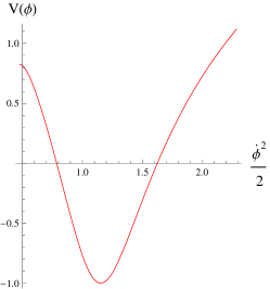
The potential and kinetic energies of the scalar field play a dynamical role to study cosmic expansion. For accelerated expansion, the field Ο•italic-Ο•\phi evolves negatively and potential dominates over the kinetic energy (Ο•Λ™22<V​(Ο•)superscriptΛ™italic-Ο•22𝑉italic-Ο•\frac{\dot{\phi}^{2}}{2}<V(\phi)) whereas negative potential follows the kinetic energy for decelerated expansion of the universe (Ο•Λ™22>βˆ’V​(Ο•)superscriptΛ™italic-Ο•22𝑉italic-Ο•\frac{\dot{\phi}^{2}}{2}>-V(\phi)). Using Eq.(8), we obtain

Ο•italic-Ο•\displaystyle\phi =\displaystyle= ∫120​ϡ​(c2′​t+c3β€²)((βˆ’Ο΅c2β€²(25c2′⁣2(40c2β€²t+40c3β€²)45c1β€²t2+50(40c2β€²t+40c3β€²)45\displaystyle\int\frac{1}{20\epsilon(c^{\prime}_{{}_{2}}t+c^{\prime}_{{}_{3}})}\left(\left(-\epsilon c^{\prime}_{{}_{2}}\left(25c^{\prime 2}_{{}_{2}}(40c^{\prime}_{{}_{2}}t+40c^{\prime}_{{}_{3}})^{\frac{4}{5}}c^{\prime}_{{}_{1}}t^{2}+50(40c^{\prime}_{{}_{2}}t+40c^{\prime}_{{}_{3}})^{\frac{4}{5}}\right.\right.\right.
Γ—\displaystyle\times c2β€²c1β€²c3β€²t+25(40c2β€²t+40c3β€²)45c1β€²c3′⁣2+896c2β€²))12),\displaystyle\left.\left.\left.c^{\prime}_{{}_{2}}c^{\prime}_{{}_{1}}c^{\prime}_{{}_{3}}t+25(40c^{\prime}_{{}_{2}}t+40c^{\prime}_{{}_{3}})^{\frac{4}{5}}c^{\prime}_{{}_{1}}c^{\prime 2}_{{}_{3}}+896c^{\prime}_{{}_{2}}\right)\right)^{\frac{1}{2}}\right),
V​(Ο•)𝑉italic-Ο•\displaystyle V(\phi) =\displaystyle= 1800​(c2′⁣2​t2+2​c2′​c3′​t+c3′⁣2)[25c1β€²(5c2′⁣3t2+5c2β€²c3′⁣2+10c2′⁣2c3β€²t)(40c2β€²t\displaystyle\frac{1}{800\left(c^{\prime 2}_{{}_{2}}t^{2}+2c^{\prime}_{{}_{2}}c^{\prime}_{{}_{3}}t+c^{\prime 2}_{{}_{3}}\right)}\left[25c^{\prime}_{{}_{1}}\left(5c^{\prime 3}_{{}_{2}}t^{2}+5c^{\prime}_{{}_{2}}c^{\prime 2}_{{}_{3}}+10c^{\prime 2}_{{}_{2}}c^{\prime}_{{}_{3}}t\right)(40c^{\prime}_{{}_{2}}t\right.
+\displaystyle+ 40c3β€²)45+8c2β€²c3β€²(βˆ’200c2β€²t2+400c3β€²t)βˆ’8(48c2′⁣2+200c3′⁣3)].\displaystyle\left.40c^{\prime}_{{}_{3}})^{\frac{4}{5}}+8c^{\prime}_{{}_{2}}c^{\prime}_{{}_{3}}\left(-200c^{\prime}_{{}_{2}}t^{2}+400c^{\prime}_{{}_{3}}t\right)-8\left(48c^{\prime 2}_{{}_{2}}+200c^{\prime 3}_{{}_{3}}\right)\right].
Refer to caption
Refer to caption
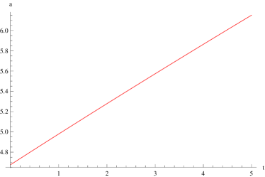
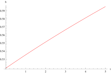
Figure 1: Plots of scale factors a​(t)π‘Žπ‘‘a(t) (left) and b​(t)𝑏𝑑b(t) (right) versus cosmic time t𝑑t for c1β€²=0.24subscriptsuperscript𝑐′10.24c^{\prime}_{{}_{1}}=0.24, c2β€²=0.45subscriptsuperscript𝑐′20.45c^{\prime}_{{}_{2}}=0.45 and c3β€²=5.5subscriptsuperscript𝑐′35.5c^{\prime}_{{}_{3}}=5.5.
Refer to caption
Refer to caption
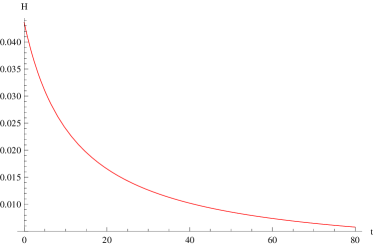
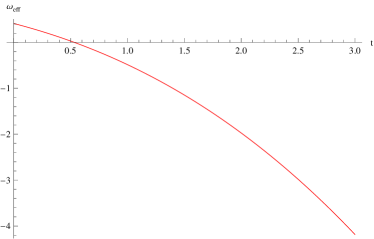
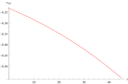
Figure 2: Plots of Hubble H​(t)𝐻𝑑H(t) (left) and EoS parameters Ο‰e​f​fsubscriptπœ”π‘’π‘“π‘“\omega_{eff} (right) versus cosmic time t𝑑t.

Figure 1 shows the graphical analysis of the scale factors for the dust case. The scale factor a​(t)π‘Žπ‘‘a(t) indicates large cosmic expansion in xπ‘₯x-direction but b​(t)𝑏𝑑b(t) represents that the universe is expanding very slowly in y𝑦y and z𝑧z-directions. Figure 2 (left plot) indicates that Hubble parameter is decreasing with the passage of time. In the right plot of Figure 2, the effective EoS parameter identifies that initially, the universe appreciates radiation dominated era and after sometime, it corresponds to dark energy era by crossing matter dominated phase.

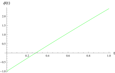
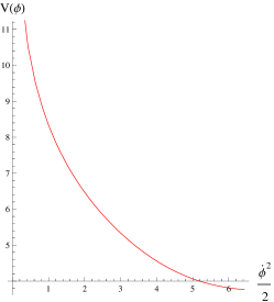
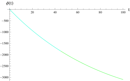
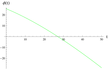
Figures 3 and 4 analyze the behavior of scalar field and cosmic expansion via phantom and quintessence models. The left plot of Figure 3 shows that the scalar field is positive initially yielding decelerated expansion but gradually, it starts increasing negatively which describes accelerated expansion. In case of quintessence model, the scalar field grows from negative to positive indicating decelerated expansion of the universe. The right plots of 3 and 4 satisfy Ο•Λ™22<V​(Ο•)superscriptΛ™italic-Ο•22𝑉italic-Ο•\frac{\dot{\phi}^{2}}{2}<V(\phi) and Ο•Λ™22>βˆ’V​(Ο•)superscriptΛ™italic-Ο•22𝑉italic-Ο•\frac{\dot{\phi}^{2}}{2}>-V(\phi) implying that phantom model yields accelerated expansion while quintessence model corresponds to decelerated expansion.
Refer to caption
Refer to caption
Figure 3: Plots of scalar field ϕ​(t)italic-ϕ𝑑\phi(t) (left) versus cosmic time t𝑑t and potential energy V​(Ο•)𝑉italic-Ο•V(\phi) versus kinetic energy Ο•Λ™22superscriptΛ™italic-Ο•22\frac{\dot{\phi}^{2}}{2} (right) for Ο΅=βˆ’1italic-Ο΅1\epsilon=-1.
Refer to caption
Refer to caption
Figure 4: Plots of scalar field ϕ​(t)italic-ϕ𝑑\phi(t) (left) versus cosmic time t𝑑t and potential energy V​(Ο•)𝑉italic-Ο•V(\phi) versus kinetic energy Ο•Λ™22superscriptΛ™italic-Ο•22\frac{\dot{\phi}^{2}}{2} (right) for Ο΅=1italic-Ο΅1\epsilon=1.

To analyze a big-rip free model, the key point is that if EoS parameter rapidly approaches to -1 and Hubble rate tends to be constant (asymptotically de Sitter universe), then it is possible to have a model in which the time required for singularity is infinite, i.e., the singularity effectively does not occur [31]. The occurrence of maximum potential of a phantom scalar field is another evident fact to avoid this singularity [32]. The graphical behavior of EoS parameter represents that Ο‰e​f​fsubscriptπœ”π‘’π‘“π‘“\omega_{eff} rapidly approaches to -1 and Hubble rate is decreasing but potential is not maximum. We may avoid the big-rip singularity in the present case if we choose c2β€²superscriptsubscript𝑐2β€²c_{2}^{\prime} to be negatively large that yields asymptotic behavior of Hubble rate.

Non-Dust Case

At large scales, perfect fluid successfully illustrates cosmic matter distribution in the presence of radiations. In the absence of boundary term and affine parameter, the coefficients of symmetry generator (20) corresponding to a,b,R,T,Ο•π‘Žπ‘π‘…π‘‡italic-Ο•a,b,R,T,\phi remain the same as in the presence of boundary term of extended symmetry. Thus, generator of Noether symmetry and associated first integrals reduce to

K𝐾\displaystyle K =\displaystyle= βˆ’2​a​c1β€‹βˆ‚βˆ‚a+c1​bβ€‹βˆ‚βˆ‚b+c2β€‹βˆ‚βˆ‚Ο•,2π‘Žsubscript𝑐1π‘Žsubscript𝑐1𝑏𝑏subscript𝑐2italic-Ο•\displaystyle-2ac_{{}_{1}}\frac{\partial}{\partial a}+c_{{}_{1}}b\frac{\partial}{\partial b}+c_{{}_{2}}\frac{\partial}{\partial\phi},
ΣΣ\displaystyle\Sigma =\displaystyle= βˆ’4​c1​a​b​b˙​fR+4​c1​b2​a˙​fR+ϡ​c2​a​b2​ϕ˙.4subscript𝑐1π‘Žπ‘Λ™π‘subscript𝑓𝑅4subscript𝑐1superscript𝑏2Λ™π‘Žsubscript𝑓𝑅italic-Ο΅subscript𝑐2π‘Žsuperscript𝑏2Λ™italic-Ο•\displaystyle-4c_{{}_{1}}ab\dot{b}f_{R}+4c_{{}_{1}}b^{2}\dot{a}f_{R}+\epsilon c_{{}_{2}}ab^{2}\dot{\phi}.

In order to formulate exact solution of dynamical equations for perfect fluid distribution, we insert Eqs.(18) and (19) into (8) and (LABEL:7) yielding

a​(t)π‘Žπ‘‘\displaystyle a(t) =\displaystyle= (5c9)25​(c2​sin⁑(c10​t)+c3​cos⁑(c10​t))45545,superscript5subscript𝑐925superscriptsubscript𝑐2subscript𝑐10𝑑subscript𝑐3subscript𝑐10𝑑45superscript545\displaystyle\frac{\left(\frac{5}{c_{{}_{9}}}\right)^{\frac{2}{5}}(c_{{}_{2}}\sin(c_{{}_{10}}t)+c_{{}_{3}}\cos(c_{{}_{10}}t))^{\frac{4}{5}}}{5^{\frac{4}{5}}},
b​(t)𝑏𝑑\displaystyle b(t) =\displaystyle= c4​(5c9)15​(c2​sin⁑(c10​t)+c3​cos⁑(c10​t))25525.subscript𝑐4superscript5subscript𝑐915superscriptsubscript𝑐2subscript𝑐10𝑑subscript𝑐3subscript𝑐10𝑑25superscript525\displaystyle\frac{c_{{}_{4}}\left(\frac{5}{c_{{}_{9}}}\right)^{\frac{1}{5}}(c_{{}_{2}}\sin(c_{{}_{10}}t)+c_{{}_{3}}\cos(c_{{}_{10}}t))^{\frac{2}{5}}}{5^{\frac{2}{5}}}.

This describes oscillatory solution of f​(R,T)𝑓𝑅𝑇f(R,T) model admitting indirect non-minimal curvature-matter coupling. To study the cosmological behavior of this solution, we consider cosmological parameters as follows
H𝐻\displaystyle H =\displaystyle= 8​c10​(c2​sin⁑(c10​t)+c3​cos⁑(c10​t))15​(c2​sin⁑(c10​t)+c3​cos⁑(c10​t)),8subscript𝑐10subscript𝑐2subscript𝑐10𝑑subscript𝑐3subscript𝑐10𝑑15subscript𝑐2subscript𝑐10𝑑subscript𝑐3subscript𝑐10𝑑\displaystyle\frac{8c_{{}_{10}}(c_{{}_{2}}\sin(c_{{}_{10}}t)+c_{{}_{3}}\cos(c_{{}_{10}}t))}{15(c_{{}_{2}}\sin(c_{{}_{10}}t)+c_{{}_{3}}\cos(c_{{}_{10}}t))},
qπ‘ž\displaystyle q =\displaystyle= βˆ’8​c22​cos2⁑(c10​t)+7​c33+8​c32​cos2⁑(c10​t)+15​c22+16​c2​c3​cos⁑(c10​t)​sin⁑(c10​t)8​(c2​sin⁑(c10​t)+c3​cos⁑(c10​t))2,8subscriptsuperscript𝑐22superscript2subscript𝑐10𝑑7subscriptsuperscript𝑐338subscriptsuperscript𝑐23superscript2subscript𝑐10𝑑15subscriptsuperscript𝑐2216subscript𝑐2subscript𝑐3subscript𝑐10𝑑subscript𝑐10𝑑8superscriptsubscript𝑐2subscript𝑐10𝑑subscript𝑐3subscript𝑐10𝑑2\displaystyle\frac{-8c^{2}_{{}_{2}}\cos^{2}(c_{{}_{10}}t)+7c^{3}_{{}_{3}}+8c^{2}_{{}_{3}}\cos^{2}(c_{{}_{10}}t)+15c^{2}_{{}_{2}}+16c_{{}_{2}}c_{{}_{3}}\cos(c_{{}_{10}}t)\sin(c_{{}_{10}}t)}{8(c_{{}_{2}}\sin(c_{{}_{10}}t)+c_{{}_{3}}\cos(c_{{}_{10}}t))^{2}},
s𝑠\displaystyle s =\displaystyle= (βˆ’45((4c24βˆ’4c34)cos2(c10t)βˆ’c34βˆ’6c22c3βˆ’5c24βˆ’(8c23c3+8c2c33)\displaystyle(-45((4c^{4}_{{}_{2}}-4c^{4}_{{}_{3}})\cos^{2}(c_{{}_{10}}t)-c^{4}_{{}_{3}}-6c^{2}_{{}_{2}}c_{{}_{3}}-5c^{4}_{{}_{2}}-(8c^{3}_{{}_{2}}c_{{}_{3}}+8c_{{}_{2}}c^{3}_{{}_{3}})
Γ—\displaystyle\times cos(c10t)sin(c10t)))/256((c24+c34βˆ’6c22c32)cos4(c10t)+(6c22c32βˆ’2c34)\displaystyle\cos(c_{{}_{10}}t)\sin(c_{{}_{10}}t)))/256((c^{4}_{{}_{2}}+c^{4}_{{}_{3}}-6c^{2}_{{}_{2}}c^{2}_{{}_{3}})\cos^{4}(c_{{}_{10}}t)+(6c^{2}_{{}_{2}}c^{2}_{{}_{3}}-2c^{4}_{{}_{3}})
Γ—\displaystyle\times cos2⁑(c10​t)+(βˆ’4​c23​c3+4​c2​c33)​sin⁑(c10​t)​cos3⁑(c10​t)βˆ’4​c2​c33​cos⁑(c10​t)superscript2subscript𝑐10𝑑4subscriptsuperscript𝑐32subscript𝑐34subscript𝑐2subscriptsuperscript𝑐33subscript𝑐10𝑑superscript3subscript𝑐10𝑑4subscript𝑐2subscriptsuperscript𝑐33subscript𝑐10𝑑\displaystyle\cos^{2}(c_{{}_{10}}t)+(-4c^{3}_{{}_{2}}c_{{}_{3}}+4c_{{}_{2}}c^{3}_{{}_{3}})\sin(c_{{}_{10}}t)\cos^{3}(c_{{}_{10}}t)-4c_{{}_{2}}c^{3}_{{}_{3}}\cos(c_{{}_{10}}t)
Γ—\displaystyle\times sin(c10t)+c34),\displaystyle\sin(c_{{}_{10}}t)+c^{4}_{{}_{3}}),
Ο‰e​f​fsubscriptπœ”π‘’π‘“π‘“\displaystyle\omega_{eff} =\displaystyle= Ο‡(3pmβˆ’Οm)+pmβˆ’Ο΅β€‹Ο•Λ™22βˆ’V(Ο•)+2​ξb2+a(3pm,aβˆ’Οm,a)+pm,aχ​(3​pmβˆ’Οm)+pm+ϡ​ϕ˙22βˆ’V​(Ο•)+2​ξb2.\displaystyle\frac{\chi(3p_{m}-\rho_{m})+p_{m}-\frac{\epsilon\dot{\phi}^{2}}{2}-V(\phi)+\frac{2\xi}{b^{2}}+a(3p_{m},_{{}_{a}}-\rho_{m},_{{}_{a}})+p_{m},_{{}_{a}}}{\chi(3p_{m}-\rho_{m})+p_{m}+\frac{\epsilon\dot{\phi}^{2}}{2}-V(\phi)+\frac{2\xi}{b^{2}}}.
Refer to caption
Refer to caption
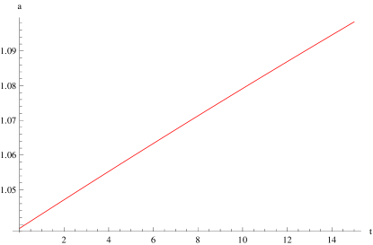
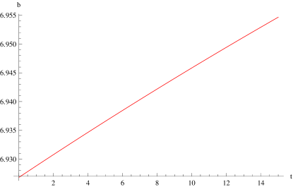
Figure 5: Plots of scale factor a​(t)π‘Žπ‘‘a(t) (left) and b​(t)𝑏𝑑b(t) (right) versus cosmic time t𝑑t for c2=c3=c9=5.5subscript𝑐2subscript𝑐3subscript𝑐95.5c_{2}=c_{3}=c_{9}=5.5 and c10=0.005subscript𝑐100.005c_{10}=0.005.
Refer to caption
Refer to caption
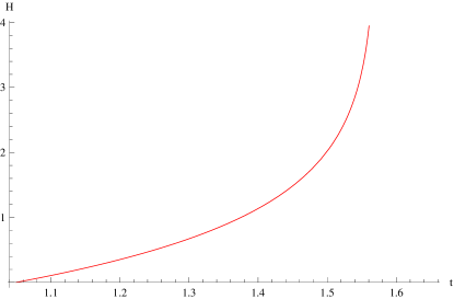
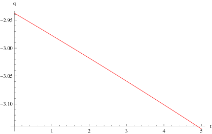
Figure 6: Plots of H​(t)𝐻𝑑H(t) (left) and q​(t)π‘žπ‘‘q(t) (right) versus cosmic time t𝑑t.

The scalar field as well as corresponding kinetic and potential energies identify the early as well as current cosmic expansion and also characterize decelerated expansion of the universe when kinetic energy dominates negative potential. In this case, Eq.(8) yields

Ο•=βˆ«Ο΅β€‹c4βˆ’5c6c22cos(2c10t)(βˆ’22F1[310,12,1310,sin[Ο€4+c10t]2]+2βˆ’2​sin⁑[2​c10​t])16​c10​cos[Ο€4+c10t]2​(c2​(cos⁑[c10​t]+sin⁑[c10​t]))2/5​d​tϡ​(c2​cos⁑[c10​t]+c2​sin⁑[c10​t])8/5,\phi=\int\frac{\epsilon c_{{}_{4}}-\frac{5c_{{}_{6}}c^{2}_{{}_{2}}\cos(2c_{{}_{10}}t)\left(-2_{2}F_{1}\left[\frac{3}{10},\frac{1}{2},\frac{13}{10},\sin\left[\frac{\pi}{4}+c_{{}_{10}}t\right]^{2}\right]+\sqrt{2-2\sin[2c_{{}_{10}}t]}\right)}{16c_{{}_{10}}\sqrt{\cos\left[\frac{\pi}{4}+c_{{}_{10}}t\right]^{2}}(c_{{}_{2}}(\cos[c_{{}_{10}}t]+\sin[c_{{}_{10}}t]))^{2/5}}dt}{\epsilon(c_{{}_{2}}\cos[c_{{}_{10}}t]+c_{{}_{2}}\sin[c_{{}_{10}}t])^{8/5}},

where F12subscriptsubscript𝐹12{}_{2}F_{1} represents hypergeometric function.
Refer to caption
Refer to caption
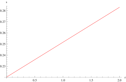
Figure 7: Plot of Ο‰e​f​fsubscriptπœ”π‘’π‘“π‘“\omega_{eff} and rβˆ’sπ‘Ÿπ‘ r-s parameters versus cosmic time t𝑑t for c2=c3=5.5subscript𝑐2subscript𝑐35.5c_{2}=c_{3}=5.5 and c10=0.005subscript𝑐100.005c_{10}=0.005.
Refer to caption
Refer to caption
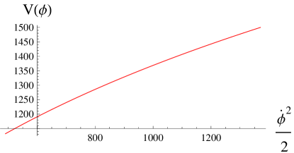
Figure 8: Plots of scalar field ϕ​(t)italic-ϕ𝑑\phi(t) (left) versus cosmic time t𝑑t and potential energy V​(Ο•)𝑉italic-Ο•V(\phi) versus kinetic energy Ο•Λ™22superscriptΛ™italic-Ο•22\frac{\dot{\phi}^{2}}{2} (right) for c2=5.5subscript𝑐25.5c_{2}=5.5, c4=βˆ’103subscript𝑐4superscript103c_{4}=-10^{3}, c6=0.5subscript𝑐60.5c_{6}=0.5 and c10=0.005subscript𝑐100.005c_{10}=0.005.

In Figure 5, the right plot shows that the universe experiences immense amount of expansion in y𝑦y and z𝑧z-directions whereas the left plot yields a small amount of expansion in xπ‘₯x-direction. Figure 6 provides information about increasing rate of expansion through Hubble parameter while negatively increasing deceleration parameter assures accelerated cosmic expansion. The left plot of Figure 7 characterizes quintessence phase of dark energy era while the right plot identifies the rβˆ’sπ‘Ÿπ‘ r-s parameters trajectories in quintessence and phantom phases as s>0𝑠0s>0 when r<1π‘Ÿ1r<1. Both plots of Figure 8 verify the current cosmic expansion for quintessence as well as phantom models as Ο•italic-Ο•\phi continuously increasing negatively and potential energy of the field is dominating over kinetic energy. The graphical interpretation of EoS parameter yields Ο‰e​f​f<βˆ’1subscriptπœ”π‘’π‘“π‘“1\omega_{eff}<-1 which is not a sufficient condition for the existence of singularity as potential turns out to be maximum with the passage of time. Thus, we may avoid big-rip singularity if Hubble rate decreases asymptotically in the presence of minimal coupling of f​(R,T)𝑓𝑅𝑇f(R,T) gravity with scalar field.

3.2 f​(R,T)𝑓𝑅𝑇f(R,T)=F​(R)+h​(R)​g​(T)πΉπ‘…β„Žπ‘…π‘”π‘‡F(R)+h(R)g(T)

To analyze the effect of direct non-minimal curvature-matter coupling, we consider this model and evaluate symmetry generators as well as associated conservation laws. Inserting the model in Eqs.(A2)-(A4), (A10), (A11) and (A15) and using separation of variables approach, we obtain

β𝛽\displaystyle\beta =\displaystyle= βˆ’b​α2​a+ϕ​Y1​(t,a,b)+Y2​(t,a,b),𝑏𝛼2π‘Žitalic-Ο•subscriptπ‘Œ1π‘‘π‘Žπ‘subscriptπ‘Œ2π‘‘π‘Žπ‘\displaystyle-\frac{b\alpha}{2a}+\phi Y_{1}(t,a,b)+Y_{2}(t,a,b),
F​(R)𝐹𝑅\displaystyle F(R) =\displaystyle= Ο΅4​d3​(βˆ’d3​Y12​(R)+d2​Y9​(R))+d5​R+d6,italic-Ο΅4subscript𝑑3subscript𝑑3subscriptπ‘Œ12𝑅subscript𝑑2subscriptπ‘Œ9𝑅subscript𝑑5𝑅subscript𝑑6\displaystyle\frac{\epsilon}{4d_{3}}\left(-d_{3}Y_{12}(R)+d_{2}Y_{9}(R)\right)+d_{5}R+d_{6},
h​(R)β„Žπ‘…\displaystyle h(R) =\displaystyle= βˆ’Ο΅4​d3(βˆ’d3Y9(R),R+d1R)+d4,g(T)=d2+d3Y10(T),\displaystyle-\frac{\epsilon}{4d_{3}}\left(-d_{3}Y_{9}(R),_{{}_{R}}+d_{1}R\right)+d_{4},\quad g(T)=d_{2}+d_{3}Y_{10}(T),
Ξ·πœ‚\displaystyle\eta =\displaystyle= 1b[Y1(t,a,b)(Y10(T)(d1+Y9(R),R)βˆ’Ο•2+Y12(R),R)+bϕτ,tβˆ’2Ο•\displaystyle\frac{1}{b}\left[Y_{1}(t,a,b)(Y_{10}(T)(d_{1}+Y_{9}(R),_{{}_{R}})-\phi^{2}+Y_{12}(R),_{{}_{R}})+b\phi\tau,_{{}_{t}}-2\phi\right.
Γ—\displaystyle\times Y2(t,a,b)+bY14(t,a,b)],\displaystyle\left.Y_{2}(t,a,b)+bY_{14}(t,a,b)\right],

where disubscript𝑑𝑖d_{i}’s (i=1​…​7𝑖1…7i=1...7) denote constants. We substitute these values in Eqs.(A1), (A8) and (A9) which yield

Ο„πœ\displaystyle\tau =\displaystyle= βˆ«βˆ’Y23​(t)Ο΅dt+d8t+d9,B=16​d4[6ab(Y19(T)d1+d4ϡϕ2\displaystyle\int-\frac{Y_{23}(t)}{\epsilon}dt+d_{8}t+d_{9},\quad B=\frac{1}{6d_{4}}\left[6ab(Y_{19}(T)d_{1}+d_{4}\epsilon\phi^{2}\right.
+\displaystyle+ Y19(T)d4eβˆ’R)Y2(t,a,b),t+6abΟ•(13d4ϡϕ2+Y19(T)d4eβˆ’R+Y19(T)\displaystyle\left.Y_{19}(T)d_{4}e^{-R})Y_{2}(t,a,b),_{{}_{t}}+6ab\phi(\frac{1}{3}d_{4}\epsilon\phi^{2}+Y_{19}(T)d_{4}e^{-R}+Y_{19}(T)\right.
Γ—\displaystyle\times d1)Y16(t,b),t+3d4(2Y22(t,a,b)+2Ο•Y21(t,a,b),t+ab2Ο•2Y23(t),t)],\displaystyle\left.d_{1})Y_{16}(t,b),_{{}_{t}}+3d_{4}(2Y_{22}(t,a,b)+2\phi Y_{21}(t,a,b),_{{}_{t}}+ab^{2}\phi^{2}Y_{23}(t),_{{}_{t}})\right],
Y1​(t,a,b)subscriptπ‘Œ1π‘‘π‘Žπ‘\displaystyle Y_{1}(t,a,b) =\displaystyle= Y16​(t,b)+Y15​(a,b)Y10​(T)=βˆ’Y19​(T)​d3+ϡ​d2​d4ϡ​d3​d4,subscriptπ‘Œ16𝑑𝑏subscriptπ‘Œ15π‘Žπ‘subscriptπ‘Œ10𝑇subscriptπ‘Œ19𝑇subscript𝑑3italic-Ο΅subscript𝑑2subscript𝑑4italic-Ο΅subscript𝑑3subscript𝑑4\displaystyle Y_{16}(t,b)+Y_{15}(a,b)\quad Y_{10}(T)=-\frac{Y_{19}(T)d_{3}+\epsilon d_{2}d_{4}}{\epsilon d_{3}d_{4}},
Y12​(R)subscriptπ‘Œ12𝑅\displaystyle Y_{12}(R) =\displaystyle= βˆ’d2​d4​eβˆ’Rd3+d6​R+d7,Y9​(R)=βˆ’eβˆ’R​d4βˆ’2​d1​R+d2,subscript𝑑2subscript𝑑4superscript𝑒𝑅subscript𝑑3subscript𝑑6𝑅subscript𝑑7subscriptπ‘Œ9𝑅superscript𝑒𝑅subscript𝑑42subscript𝑑1𝑅subscript𝑑2\displaystyle-\frac{d_{2}d_{4}e^{-R}}{d_{3}}+d_{6}R+d_{7},\quad Y_{9}(R)=-e^{-R}d_{4}-2d_{1}R+d_{2},
Y14​(t,a,b)subscriptπ‘Œ14π‘‘π‘Žπ‘\displaystyle Y_{14}(t,a,b) =\displaystyle= βˆ’Y21​(t,a,b)b2​aβ€‹Ο΅βˆ’b​a​d2​ϡ​d1​Y16​(t,b)+d6​ϡ​b​a​d3​Y16​(t,b)ϡ​b2​a​d3+Y24​(b,a).subscriptπ‘Œ21π‘‘π‘Žπ‘superscript𝑏2π‘Žitalic-Ο΅π‘π‘Žsubscript𝑑2italic-Ο΅subscript𝑑1subscriptπ‘Œ16𝑑𝑏subscript𝑑6italic-Ο΅π‘π‘Žsubscript𝑑3subscriptπ‘Œ16𝑑𝑏italic-Ο΅superscript𝑏2π‘Žsubscript𝑑3subscriptπ‘Œ24π‘π‘Ž\displaystyle-\frac{Y_{21}(t,a,b)}{b^{2}a\epsilon}-\frac{bad_{2}\epsilon d_{1}Y_{16}(t,b)+d_{6}\epsilon bad_{3}Y_{16}(t,b)}{\epsilon b^{2}ad_{3}}+Y_{24}(b,a).

To evaluate remaining unknown functions, we insert the above functions into Ξ²,Ξ·,F,g,hπ›½πœ‚πΉπ‘”β„Ž\beta,~{}\eta,~{}F,~{}g,~{}h and solve Eqs.(A5)-(A7) with (A12)-(A14) and (A16)-(A21) leading to

Y21​(t,a,b)subscriptπ‘Œ21π‘‘π‘Žπ‘\displaystyle Y_{21}(t,a,b) =\displaystyle= Y26​(a,b),Y22​(t,a,b)=d10​t,Y16​(t,b)=βˆ’d12​b,formulae-sequencesubscriptπ‘Œ26π‘Žπ‘subscriptπ‘Œ22π‘‘π‘Žπ‘subscript𝑑10𝑑subscriptπ‘Œ16𝑑𝑏subscript𝑑12𝑏\displaystyle Y_{26}(a,b),\quad Y_{22}(t,a,b)=d_{10}t,\quad Y_{16}(t,b)=-d_{12}b,
Y15​(a,b)subscriptπ‘Œ15π‘Žπ‘\displaystyle Y_{15}(a,b) =\displaystyle= d12​b,Y24​(b,a)=0,Y2​(t,a,b)=d9​b,formulae-sequencesubscript𝑑12𝑏subscriptπ‘Œ24π‘π‘Ž0subscriptπ‘Œ2π‘‘π‘Žπ‘subscript𝑑9𝑏\displaystyle d_{12}b,\quad Y_{24}(b,a)=0,\quad Y_{2}(t,a,b)=d_{9}b,
Y23​(t)subscriptπ‘Œ23𝑑\displaystyle Y_{23}(t) =\displaystyle= ϡ​(βˆ’2​d9+eβˆ’R​d4​d3​d11​eR+d8),Ξ΄=0,Ξ³=d11​eR​Td1​3formulae-sequenceitalic-Ο΅2subscript𝑑9superscript𝑒𝑅subscript𝑑4subscript𝑑3subscript𝑑11superscript𝑒𝑅subscript𝑑8𝛿0𝛾subscript𝑑11superscript𝑒𝑅𝑇subscript𝑑13\displaystyle\epsilon(-2d_{9}+e^{-R}d_{4}d_{3}d_{11}e^{R}+d_{8}),\quad\delta=0,\quad\gamma=\frac{d_{11}e^{R}T}{d_{1}3}
Γ—\displaystyle\times (eβˆ’R​d4​T​d13​d3βˆ’d1​d13​d3​T+(2​((βˆ’2​d5+12​ϡ​d6)​d3+d1​d2​ϡ))​d4).superscript𝑒𝑅subscript𝑑4𝑇subscript𝑑13subscript𝑑3subscript𝑑1subscript𝑑13subscript𝑑3𝑇22subscript𝑑512italic-Ο΅subscript𝑑6subscript𝑑3subscript𝑑1subscript𝑑2italic-Ο΅subscript𝑑4\displaystyle(e^{-R}d_{4}Td_{13}d_{3}-d_{1}d_{13}d_{3}T+(2((-2d_{5}+\frac{1}{2}\epsilon d_{6})d_{3}+d_{1}d_{2}\epsilon))d_{4}).

Using these solutions in Eq.(A22) with d11subscript𝑑11d_{11}=0 and d6=d2​d1d3subscript𝑑6subscript𝑑2subscript𝑑1subscript𝑑3d_{6}=\frac{d_{2}d_{1}}{d_{3}}, it follows that

Ο„πœ\displaystyle\tau =\displaystyle= 3​d9,Ξ±=d10​a,Ξ²=b​(d9βˆ’d102),Ξ΄=0,Ξ³=0,formulae-sequence3subscript𝑑9𝛼subscript𝑑10π‘Žformulae-sequence𝛽𝑏subscript𝑑9subscript𝑑102formulae-sequence𝛿0𝛾0\displaystyle 3d_{9},\quad\alpha=d_{10}a,\quad\beta=b(d_{9}-\frac{d_{10}}{2}),\quad\delta=0,\quad\gamma=0,
B𝐡\displaystyle B =\displaystyle= d10​t,Ξ·=βˆ’d1Ο΅+2​d12​d6,F​(R)=d6+d5​Rβˆ’3​d6​ϡ​R4,formulae-sequencesubscript𝑑10π‘‘πœ‚subscript𝑑1italic-Ο΅2subscript𝑑12subscript𝑑6𝐹𝑅subscript𝑑6subscript𝑑5𝑅3subscript𝑑6italic-ϡ𝑅4\displaystyle d_{10}t,\quad\eta=-\frac{d_{1}}{\epsilon}+2d_{12}d_{6},\quad F(R)=d_{6}+d_{5}R-\frac{3d_{6}\epsilon R}{4},
h​(R)β„Žπ‘…\displaystyle h(R) =\displaystyle= d4βˆ’Ο΅4​d3​(d4​eβˆ’R+d1​Rβˆ’2​d1),g​(T)=d2βˆ’d2​d4β€‹Ο΅βˆ’d3​d13​Td4​ϡ.subscript𝑑4italic-Ο΅4subscript𝑑3subscript𝑑4superscript𝑒𝑅subscript𝑑1𝑅2subscript𝑑1𝑔𝑇subscript𝑑2subscript𝑑2subscript𝑑4italic-Ο΅subscript𝑑3subscript𝑑13𝑇subscript𝑑4italic-Ο΅\displaystyle d_{4}-\frac{\epsilon}{4d_{3}}(d_{4}e^{-R}+d_{1}R-2d_{1}),\quad g(T)=d_{2}-\frac{d_{2}d_{4}\epsilon-d_{3}d_{13}T}{d_{4}\epsilon}.

Inserting F,hπΉβ„ŽF,~{}h and g𝑔g, the f​(R,T)𝑓𝑅𝑇f(R,T) model becomes

f​(R,T)=βˆ’3​ϡ​d6​R4+d5​R+d6+(d4βˆ’Ο΅4​d3​(d4​eβˆ’R+d1​Rβˆ’2​d1))​(d3​d13​Td4​ϡ).𝑓𝑅𝑇3italic-Ο΅subscript𝑑6𝑅4subscript𝑑5𝑅subscript𝑑6subscript𝑑4italic-Ο΅4subscript𝑑3subscript𝑑4superscript𝑒𝑅subscript𝑑1𝑅2subscript𝑑1subscript𝑑3subscript𝑑13𝑇subscript𝑑4italic-Ο΅f(R,T)=-\frac{3\epsilon d_{6}R}{4}+d_{5}R+d_{6}+(d_{4}-\frac{\epsilon}{4d_{3}}(d_{4}e^{-R}+d_{1}R-2d_{1}))(\frac{d_{3}d_{13}T}{d_{4}\epsilon}).

Thus, the constructed model also experiences a direct coupling between curvature and matter parts. In this case, the symmetry generators and associated conserved quantities are

K1subscript𝐾1\displaystyle K_{1} =\displaystyle= 3βˆ‚βˆ‚t+bβˆ‚βˆ‚b,Ξ£1=14​d3​ϡ(βˆ’4ab2Ο΅2d3Ο•Λ™2+4d10d3Ο΅t+3tab2d1RTd3Ο΅\displaystyle 3\frac{\partial}{\partial t}+b\frac{\partial}{\partial b},\quad\Sigma_{1}=\frac{1}{4d_{3}\epsilon}(-4ab^{2}\epsilon^{2}d_{3}\dot{\phi}^{2}+4d_{10}d_{3}\epsilon t+3tab^{2}d_{1}RTd_{3}\epsilon
βˆ’\displaystyle- 9​t​a​b2​d1​R​pm​d3​ϡ+3​t​a​b2​d1​R​ρm​d3β€‹Ο΅βˆ’12​t​d1​T​a˙​b˙​b​d3β€‹Ο΅βˆ’4​b2​d4​T9π‘‘π‘Žsuperscript𝑏2subscript𝑑1𝑅subscriptπ‘π‘šsubscript𝑑3italic-Ο΅3π‘‘π‘Žsuperscript𝑏2subscript𝑑1𝑅subscriptπœŒπ‘šsubscript𝑑3italic-Ο΅12𝑑subscript𝑑1π‘‡Λ™π‘ŽΛ™π‘π‘subscript𝑑3italic-Ο΅4superscript𝑏2subscript𝑑4𝑇\displaystyle 9tab^{2}d_{1}Rp_{m}d_{3}\epsilon+3tab^{2}d_{1}R\rho_{m}d_{3}\epsilon-12td_{1}T\dot{a}\dot{b}bd_{3}\epsilon-4b^{2}d_{4}T
Γ—\displaystyle\times a˙​eβˆ’R​d3β€‹Ο΅βˆ’4​b2​a​T˙​d4​eβˆ’R​d3β€‹Ο΅βˆ’9​t​a​b2​d4​pm​eβˆ’R​d3​ϡ+3​t​a​b2​d4​ρmΛ™π‘Žsuperscript𝑒𝑅subscript𝑑3italic-Ο΅4superscript𝑏2π‘ŽΛ™π‘‡subscript𝑑4superscript𝑒𝑅subscript𝑑3italic-Ο΅9π‘‘π‘Žsuperscript𝑏2subscript𝑑4subscriptπ‘π‘šsuperscript𝑒𝑅subscript𝑑3italic-Ο΅3π‘‘π‘Žsuperscript𝑏2subscript𝑑4subscriptπœŒπ‘š\displaystyle\dot{a}e^{-R}d_{3}\epsilon-4b^{2}a\dot{T}d_{4}e^{-R}d_{3}\epsilon-9tab^{2}d_{4}p_{m}e^{-R}d_{3}\epsilon+3tab^{2}d_{4}\rho_{m}
Γ—\displaystyle\times eβˆ’R​d3​ϡ+6​t​d4​T​a​bΛ™2​eβˆ’R​d3​ϡ+6​t​d4​T​a​q​eβˆ’R​d3β€‹Ο΅βˆ’4​b​d4​T​a​b˙​eβˆ’R​d3​ϡsuperscript𝑒𝑅subscript𝑑3italic-Ο΅6𝑑subscript𝑑4π‘‡π‘Žsuperscript˙𝑏2superscript𝑒𝑅subscript𝑑3italic-Ο΅6𝑑subscript𝑑4π‘‡π‘Žπ‘žsuperscript𝑒𝑅subscript𝑑3italic-Ο΅4𝑏subscript𝑑4π‘‡π‘ŽΛ™π‘superscript𝑒𝑅subscript𝑑3italic-Ο΅\displaystyle e^{-R}d_{3}\epsilon+6td_{4}Ta\dot{b}^{2}e^{-R}d_{3}\epsilon+6td_{4}Taqe^{-R}d_{3}\epsilon-4bd_{4}Ta\dot{b}e^{-R}d_{3}\epsilon
+\displaystyle+ 4​b2​a​R˙​d4​T​eβˆ’R​d3​ϡ+4​b2​a​T˙​d1​d3β€‹Ο΅βˆ’12​t​a​b2​d2​d1β€‹Ο΅βˆ’12​t​a​b2​pm4superscript𝑏2π‘ŽΛ™π‘…subscript𝑑4𝑇superscript𝑒𝑅subscript𝑑3italic-Ο΅4superscript𝑏2π‘ŽΛ™π‘‡subscript𝑑1subscript𝑑3italic-Ο΅12π‘‘π‘Žsuperscript𝑏2subscript𝑑2subscript𝑑1italic-Ο΅12π‘‘π‘Žsuperscript𝑏2subscriptπ‘π‘š\displaystyle 4b^{2}a\dot{R}d_{4}Te^{-R}d_{3}\epsilon+4b^{2}a\dot{T}d_{1}d_{3}\epsilon-12tab^{2}d_{2}d_{1}\epsilon-12tab^{2}p_{m}
Γ—\displaystyle\times d3​ϡ+12​t​a​b2​V​(Ο•)​d3β€‹Ο΅βˆ’24​t​d5​a​b˙​d3β€‹Ο΅βˆ’24​t​d5​a​q​d3​ϡ+16​b​d5​a​bΛ™subscript𝑑3italic-Ο΅12π‘‘π‘Žsuperscript𝑏2𝑉italic-Ο•subscript𝑑3italic-Ο΅24𝑑subscript𝑑5π‘ŽΛ™π‘subscript𝑑3italic-Ο΅24𝑑subscript𝑑5π‘Žπ‘žsubscript𝑑3italic-Ο΅16𝑏subscript𝑑5π‘ŽΛ™π‘\displaystyle d_{3}\epsilon+12tab^{2}V(\phi)d_{3}\epsilon-24td_{5}a\dot{b}d_{3}\epsilon-24td_{5}aqd_{3}\epsilon+16bd_{5}a\dot{b}
Γ—\displaystyle\times d3​ϡ+36​t​a​b2​d32​d4​pmβˆ’12​t​a​b2​d32​d4​ρm+18​t​ϡ2​d2​d1​a​bΛ™2+18​t​ϡ2subscript𝑑3italic-Ο΅36π‘‘π‘Žsuperscript𝑏2superscriptsubscript𝑑32subscript𝑑4subscriptπ‘π‘š12π‘‘π‘Žsuperscript𝑏2superscriptsubscript𝑑32subscript𝑑4subscriptπœŒπ‘š18𝑑superscriptitalic-Ο΅2subscript𝑑2subscript𝑑1π‘Žsuperscript˙𝑏218𝑑superscriptitalic-Ο΅2\displaystyle d_{3}\epsilon+36tab^{2}d_{3}^{2}d_{4}p_{m}-12tab^{2}d_{3}^{2}d_{4}\rho_{m}+18t\epsilon^{2}d_{2}d_{1}a\dot{b}^{2}+18t\epsilon^{2}
Γ—\displaystyle\times d2​d1​a​qβˆ’12​b​ϡ2​d2​d1​a​bΛ™+4​b2​d1​T​a˙​d3β€‹Ο΅βˆ’12​b2​ϡ2​d2​d1​aΛ™+16​b2​d5subscript𝑑2subscript𝑑1π‘Žπ‘ž12𝑏superscriptitalic-Ο΅2subscript𝑑2subscript𝑑1π‘ŽΛ™π‘4superscript𝑏2subscript𝑑1π‘‡Λ™π‘Žsubscript𝑑3italic-Ο΅12superscript𝑏2superscriptitalic-Ο΅2subscript𝑑2subscript𝑑1Λ™π‘Ž16superscript𝑏2subscript𝑑5\displaystyle d_{2}d_{1}aq-12b\epsilon^{2}d_{2}d_{1}a\dot{b}+4b^{2}d_{1}T\dot{a}d_{3}\epsilon-12b^{2}\epsilon^{2}d_{2}d_{1}\dot{a}+16b^{2}d_{5}
Γ—\displaystyle\times a˙​d3β€‹Ο΅βˆ’3​t​a​b2​R​d4​T​eβˆ’R​d3​ϡ+12​t​d4​T​a˙​b˙​b​eβˆ’R​d3​ϡ+36​t​ϡ2​d2​d1​a˙​b˙​bΛ™π‘Žsubscript𝑑3italic-Ο΅3π‘‘π‘Žsuperscript𝑏2𝑅subscript𝑑4𝑇superscript𝑒𝑅subscript𝑑3italic-Ο΅12𝑑subscript𝑑4π‘‡Λ™π‘ŽΛ™π‘π‘superscript𝑒𝑅subscript𝑑3italic-Ο΅36𝑑superscriptitalic-Ο΅2subscript𝑑2subscript𝑑1Λ™π‘ŽΛ™π‘π‘\displaystyle\dot{a}d_{3}\epsilon-3tab^{2}Rd_{4}Te^{-R}d_{3}\epsilon+12td_{4}T\dot{a}\dot{b}be^{-R}d_{3}\epsilon+36t\epsilon^{2}d_{2}d_{1}\dot{a}\dot{b}b
+\displaystyle+ 4​b​d1​T​a​b˙​d3​ϡ+6​t​a​b2​e​ϕ˙2​d3​ϡ+18​t​a​b2​d1​pm​d3β€‹Ο΅βˆ’6​t​a​b2​d1​ρm​d3​ϡ4𝑏subscript𝑑1π‘‡π‘ŽΛ™π‘subscript𝑑3italic-Ο΅6π‘‘π‘Žsuperscript𝑏2𝑒superscriptΛ™italic-Ο•2subscript𝑑3italic-Ο΅18π‘‘π‘Žsuperscript𝑏2subscript𝑑1subscriptπ‘π‘šsubscript𝑑3italic-Ο΅6π‘‘π‘Žsuperscript𝑏2subscript𝑑1subscriptπœŒπ‘šsubscript𝑑3italic-Ο΅\displaystyle 4bd_{1}Ta\dot{b}d_{3}\epsilon+6tab^{2}e\dot{\phi}^{2}d_{3}\epsilon+18tab^{2}d_{1}p_{m}d_{3}\epsilon-6tab^{2}d_{1}\rho_{m}d_{3}\epsilon
βˆ’\displaystyle- 48td5aΛ™bΛ™bd3Ο΅βˆ’6td1TabΛ™2d3Ο΅βˆ’6td1Taqd3Ο΅),\displaystyle 48td_{5}\dot{a}\dot{b}bd_{3}\epsilon-6td_{1}Ta\dot{b}^{2}d_{3}\epsilon-6td_{1}Taqd_{3}\epsilon),
K2subscript𝐾2\displaystyle K_{2} =\displaystyle= aβˆ‚βˆ‚aβˆ’b2βˆ‚βˆ‚b,Ξ£2=βˆ’b2​d3(βˆ’abΛ™d1Td3+3abΛ™Ο΅d2d1+abΛ™d4Teβˆ’Rd3\displaystyle a\frac{\partial}{\partial a}-\frac{b}{2}\frac{\partial}{\partial b},\quad\Sigma_{2}=-\frac{b}{2d_{3}}(-a\dot{b}d_{1}Td_{3}+3a\dot{b}\epsilon d_{2}d_{1}+a\dot{b}d_{4}Te^{-R}d_{3}
βˆ’\displaystyle- 4abΛ™d5d3+bd1TaΛ™d3+4bd5aΛ™d3βˆ’3bΟ΅d2d1aΛ™βˆ’bd4TaΛ™eβˆ’Rd3),\displaystyle 4a\dot{b}d_{5}d_{3}+bd_{1}T\dot{a}d_{3}+4bd_{5}\dot{a}d_{3}-3b\epsilon d_{2}d_{1}\dot{a}-bd_{4}T\dot{a}e^{-R}d_{3}),
K3subscript𝐾3\displaystyle K_{3} =\displaystyle= βˆ’1Ο΅β€‹βˆ‚βˆ‚Ο•,Ξ£3=a​b2​ϕ˙,K4=2​d12β€‹βˆ‚βˆ‚Ο•,Ξ£4=2​d12​a​b2​ϡ​ϕ˙.formulae-sequence1italic-Ο΅italic-Ο•subscriptΞ£3π‘Žsuperscript𝑏2Λ™italic-Ο•formulae-sequencesubscript𝐾42subscript𝑑12italic-Ο•subscriptΞ£42subscript𝑑12π‘Žsuperscript𝑏2italic-Ο΅Λ™italic-Ο•\displaystyle-\frac{1}{\epsilon}\frac{\partial}{\partial\phi},\quad\Sigma_{3}=ab^{2}\dot{\phi},\quad K_{4}=2d_{12}\frac{\partial}{\partial\phi},\quad\Sigma_{4}=2d_{12}ab^{2}\epsilon\dot{\phi}.

We see that scaling symmetry appears through generator K2subscript𝐾2K_{2} with the first integral Σ2subscriptΣ2\Sigma_{2} leading to conserved linear momentum.

Now we investigate the existence of Noether symmetry in the absence of affine parameter and boundary term of the extended symmetry and also study the effect of direct curvature-matter coupling on conservation laws. For this purpose, we solve Eqs.(A5), (A6), (A9) and (A12)-(A21) which give

δ𝛿\displaystyle\delta =\displaystyle= βˆ’a2Y9(T),T(13Y4(a,b),aΟ•3+2Y4(a,b),aY9(T)Ο•+2Y4(a,b),aY8(b)Ο•\displaystyle-\frac{a}{2Y_{9}(T),_{{}_{T}}}(\frac{1}{3}Y_{4}(a,b),_{{}_{a}}\phi^{3}+2Y_{4}(a,b),_{{}_{a}}Y_{9}(T)\phi+2Y_{4}(a,b),_{{}_{a}}Y_{8}(b)\phi
+\displaystyle+ Ο•2Y5(a,b),a+2Y7(a,b),aΟ•)+Y12(a,R,T,b),F(R)=k4R+k5,\displaystyle\phi^{2}Y_{5}(a,b),_{{}_{a}}+2Y_{7}(a,b),_{{}_{a}}\phi)+Y_{12}(a,R,T,b),\quad F(R)=k_{4}R+k_{5},
β𝛽\displaystyle\beta =\displaystyle= βˆ’b2​a​(Y10​(a,R,T,b)+a​Y5​(a,b)),g​(T)=k1+Y9​(T)​k2𝑏2π‘Žsubscriptπ‘Œ10π‘Žπ‘…π‘‡π‘π‘Žsubscriptπ‘Œ5π‘Žπ‘π‘”π‘‡subscriptπ‘˜1subscriptπ‘Œ9𝑇subscriptπ‘˜2\displaystyle-\frac{b}{2a}(Y_{10}(a,R,T,b)+aY_{5}(a,b)),\quad g(T)=k_{1}+Y_{9}(T)k_{2}
Ξ·πœ‚\displaystyle\eta =\displaystyle= 12​(Ο•2+2​Y9​(T)+2​Y8​(b))​Y4​(a,b)+Y5​(a,b)​ϕ+Y7​(b,a),12superscriptitalic-Ο•22subscriptπ‘Œ9𝑇2subscriptπ‘Œ8𝑏subscriptπ‘Œ4π‘Žπ‘subscriptπ‘Œ5π‘Žπ‘italic-Ο•subscriptπ‘Œ7π‘π‘Ž\displaystyle\frac{1}{2}(\phi^{2}+2Y_{9}(T)+2Y_{8}(b))Y_{4}(a,b)+Y_{5}(a,b)\phi+Y_{7}(b,a),
h​(R)β„Žπ‘…\displaystyle h(R) =\displaystyle= ϡ​R2​(k2+k3),Ξ³=Y11​(a,b,R,T),italic-ϡ𝑅2subscriptπ‘˜2subscriptπ‘˜3𝛾subscriptπ‘Œ11π‘Žπ‘π‘…π‘‡\displaystyle\frac{\epsilon R}{2(k_{2}+k_{3})},\quad\gamma=Y_{11}(a,b,R,T),
α𝛼\displaystyle\alpha =\displaystyle= βˆ’Y4​(a,b)​a​ϕ+Y10​(a,b,R,T),subscriptπ‘Œ4π‘Žπ‘π‘Žitalic-Ο•subscriptπ‘Œ10π‘Žπ‘π‘…π‘‡\displaystyle-Y_{4}(a,b)a\phi+Y_{10}(a,b,R,T),

where klsubscriptπ‘˜π‘™k_{l}’s (l=1​…​5𝑙1…5l=1...5) are arbitrary constants. Inserting these solutions into the remaining equations of the system, we obtain

V​(Ο•)𝑉italic-Ο•\displaystyle V(\phi) =\displaystyle= k10​ϕ+k11,Y10​(a,R,T,b)=k8​a,Y4​(a,b)=0,formulae-sequencesubscriptπ‘˜10italic-Ο•subscriptπ‘˜11subscriptπ‘Œ10π‘Žπ‘…π‘‡π‘subscriptπ‘˜8π‘Žsubscriptπ‘Œ4π‘Žπ‘0\displaystyle k_{10}\phi+k_{11},\quad Y_{10}(a,R,T,b)=k_{8}a,\quad Y_{4}(a,b)=0,
Y12​(a,R,T,b)subscriptπ‘Œ12π‘Žπ‘…π‘‡π‘\displaystyle Y_{12}(a,R,T,b) =\displaystyle= βˆ’k82​k2​((ϡ​(k6​T+k7)+2​k4)​k2+ϡ​k1),Y5​(a,b)=βˆ’k6​k8​ϡ2,subscriptπ‘˜82subscriptπ‘˜2italic-Ο΅subscriptπ‘˜6𝑇subscriptπ‘˜72subscriptπ‘˜4subscriptπ‘˜2italic-Ο΅subscriptπ‘˜1subscriptπ‘Œ5π‘Žπ‘subscriptπ‘˜6subscriptπ‘˜8italic-Ο΅2\displaystyle-\frac{k_{8}}{2k_{2}}((\epsilon(k_{6}T+k_{7})+2k_{4})k_{2}+\epsilon k_{1}),\quad Y_{5}(a,b)=-\frac{k_{6}k_{8}\epsilon}{2},
Y7​(b,a)subscriptπ‘Œ7π‘π‘Ž\displaystyle Y_{7}(b,a) =\displaystyle= k9,Y9​(T)=k6​T+k7,subscriptπ‘˜9subscriptπ‘Œ9𝑇subscriptπ‘˜6𝑇subscriptπ‘˜7\displaystyle k_{9},\quad Y_{9}(T)=k_{6}T+k_{7},
pmsubscriptπ‘π‘š\displaystyle p_{m} =\displaystyle= 2​k9​k10ϡ​k8​k6βˆ’k5+k11+2​k2​k4​k3Ο΅+aβˆ’k6​ϡ2​ϡ​k6​b​a12βˆ’Ο΅β€‹k64,2subscriptπ‘˜9subscriptπ‘˜10italic-Ο΅subscriptπ‘˜8subscriptπ‘˜6subscriptπ‘˜5subscriptπ‘˜112subscriptπ‘˜2subscriptπ‘˜4subscriptπ‘˜3italic-Ο΅superscriptπ‘Žsubscriptπ‘˜6italic-Ο΅2italic-Ο΅subscriptπ‘˜6𝑏superscriptπ‘Ž12italic-Ο΅subscriptπ‘˜64\displaystyle\frac{2k_{9}k_{10}}{\epsilon k_{8}k_{6}}-k_{5}+k_{11}+\frac{2k_{2}k_{4}k_{3}}{\epsilon}+a^{-\frac{k_{6}\epsilon}{2}}\epsilon k_{6}ba^{\frac{1}{2}-\frac{\epsilon k_{6}}{4}},
ρmsubscriptπœŒπ‘š\displaystyle\rho_{m} =\displaystyle= k7k6+6​k2​k4​k3Ο΅βˆ’3​k5+3​k11+2​k4k6​ϡ+6​k9​k10k8​k6​ϡ+k1k2​k6subscriptπ‘˜7subscriptπ‘˜66subscriptπ‘˜2subscriptπ‘˜4subscriptπ‘˜3italic-Ο΅3subscriptπ‘˜53subscriptπ‘˜112subscriptπ‘˜4subscriptπ‘˜6italic-Ο΅6subscriptπ‘˜9subscriptπ‘˜10subscriptπ‘˜8subscriptπ‘˜6italic-Ο΅subscriptπ‘˜1subscriptπ‘˜2subscriptπ‘˜6\displaystyle\frac{k_{7}}{k_{6}}+\frac{6k_{2}k_{4}k_{3}}{\epsilon}-3k_{5}+3k_{11}+\frac{2k_{4}}{k_{6}\epsilon}+\frac{6k_{9}k_{10}}{k_{8}k_{6}\epsilon}+\frac{k_{1}}{k_{2}k_{6}}
+\displaystyle+ aβˆ’k6​ϡ2​ϡ​k6​b​a12βˆ’Ο΅β€‹k64.superscriptπ‘Žsubscriptπ‘˜6italic-Ο΅2italic-Ο΅subscriptπ‘˜6𝑏superscriptπ‘Ž12italic-Ο΅subscriptπ‘˜64\displaystyle a^{-\frac{k_{6}\epsilon}{2}}\epsilon k_{6}ba^{\frac{1}{2}-\frac{\epsilon k_{6}}{4}}.

The corresponding Noether symmetry generator with associated first integral take the form

K1subscript𝐾1\displaystyle K_{1} =\displaystyle= aβ€‹βˆ‚βˆ‚aβˆ’b2​(1βˆ’k6​ϡ2)β€‹βˆ‚βˆ‚b+Rβ€‹βˆ‚βˆ‚Rβˆ’(k1​ϡ+k2​(ϡ​(k6​T+k7)+2​k4))π‘Žπ‘Žπ‘21subscriptπ‘˜6italic-Ο΅2𝑏𝑅𝑅subscriptπ‘˜1italic-Ο΅subscriptπ‘˜2italic-Ο΅subscriptπ‘˜6𝑇subscriptπ‘˜72subscriptπ‘˜4\displaystyle a\frac{\partial}{\partial a}-\frac{b}{2}\left(1-\frac{k_{6}\epsilon}{2}\right)\frac{\partial}{\partial b}+R\frac{\partial}{\partial R}-(k_{1}\epsilon+k_{2}(\epsilon(k_{6}T+k_{7})+2k_{4}))
Γ—\displaystyle\times 12​k2β€‹βˆ‚βˆ‚Tβˆ’k6​ϡ​ϕ2β€‹βˆ‚βˆ‚Ο•,Ξ£1=a​b​b˙​ϡ​k6​Tβˆ’b2​ϡ​k1​aΛ™k2βˆ’b2​ϡ​k6​T​aΛ™βˆ’b​a​ϡ​k6​k4​bΛ™12subscriptπ‘˜2𝑇subscriptπ‘˜6italic-Ο΅italic-Ο•2italic-Ο•subscriptΞ£1π‘Žπ‘Λ™π‘italic-Ο΅subscriptπ‘˜6𝑇superscript𝑏2italic-Ο΅subscriptπ‘˜1Λ™π‘Žsubscriptπ‘˜2superscript𝑏2italic-Ο΅subscriptπ‘˜6π‘‡Λ™π‘Žπ‘π‘Žitalic-Ο΅subscriptπ‘˜6subscriptπ‘˜4˙𝑏\displaystyle\frac{1}{2k_{2}}\frac{\partial}{\partial T}-\frac{k_{6}\epsilon\phi}{2}\frac{\partial}{\partial\phi},\quad\Sigma_{1}=ab\dot{b}\epsilon k_{6}T-\frac{b^{2}\epsilon k_{1}\dot{a}}{k_{2}}-b^{2}\epsilon k_{6}T\dot{a}-ba\epsilon k_{6}k_{4}\dot{b}
βˆ’\displaystyle- b​a​ϡ2​k62​T​bΛ™2βˆ’b​a​ϡ2​k6​k7​bΛ™2+a​b​b˙​ϡ​k1k2+a​b​b˙​ϡ​k7βˆ’b​a​ϡ2​k6​k1​bΛ™2​k2βˆ’a​b2​ϡ2​ϕ˙​k6​ϕ2π‘π‘Žsuperscriptitalic-Ο΅2superscriptsubscriptπ‘˜62𝑇˙𝑏2π‘π‘Žsuperscriptitalic-Ο΅2subscriptπ‘˜6subscriptπ‘˜7˙𝑏2π‘Žπ‘Λ™π‘italic-Ο΅subscriptπ‘˜1subscriptπ‘˜2π‘Žπ‘Λ™π‘italic-Ο΅subscriptπ‘˜7π‘π‘Žsuperscriptitalic-Ο΅2subscriptπ‘˜6subscriptπ‘˜1˙𝑏2subscriptπ‘˜2π‘Žsuperscript𝑏2superscriptitalic-Ο΅2Λ™italic-Ο•subscriptπ‘˜6italic-Ο•2\displaystyle\frac{ba\epsilon^{2}k_{6}^{2}T\dot{b}}{2}-\frac{ba\epsilon^{2}k_{6}k_{7}\dot{b}}{2}+\frac{ab\dot{b}\epsilon k_{1}}{k_{2}}+ab\dot{b}\epsilon k_{7}-\frac{ba\epsilon^{2}k_{6}k_{1}\dot{b}}{2k_{2}}-\frac{ab^{2}\epsilon^{2}\dot{\phi}k_{6}\phi}{2}
+\displaystyle+ 2​a​b​b˙​k4βˆ’2​b2​k4​aΛ™βˆ’b2​ϡ​k7​aΛ™+b2​a​ϡ2​k62​TΛ™2,2π‘Žπ‘Λ™π‘subscriptπ‘˜42superscript𝑏2subscriptπ‘˜4Λ™π‘Žsuperscript𝑏2italic-Ο΅subscriptπ‘˜7Λ™π‘Žsuperscript𝑏2π‘Žsuperscriptitalic-Ο΅2superscriptsubscriptπ‘˜62˙𝑇2\displaystyle 2ab\dot{b}k_{4}-2b^{2}k_{4}\dot{a}-b^{2}\epsilon k_{7}\dot{a}+\frac{b^{2}a\epsilon^{2}k_{6}^{2}\dot{T}}{2},
K2subscript𝐾2\displaystyle K_{2} =\displaystyle= βˆ‚βˆ‚Ο•,Ξ£2=a​b2​ϡ​ϕ˙​k9.italic-Ο•subscriptΞ£2π‘Žsuperscript𝑏2italic-Ο΅Λ™italic-Ο•subscriptπ‘˜9\displaystyle\frac{\partial}{\partial\phi},\quad\Sigma_{2}=ab^{2}\epsilon\dot{\phi}k_{9}.

Here the symmetry generator K1subscript𝐾1K_{1} yields scaling symmetry.

4 Final Remarks

In this paper, we have analyzed the existence of Noether symmetry in a non-minimally coupled f​(R,T)𝑓𝑅𝑇f(R,T) gravity interacting with scalar field model for anisotropic homogeneous universe models like BI, BIII and KS models. Using Noether symmetry approach, we have found conserved quantities associated with symmetry generators and studied the contribution of direct as well as indirect curvature-matter coupling through two f​(R,T)𝑓𝑅𝑇f(R,T) models. We have also formulated exact solutions for dust and perfect fluid distributions whose cosmological analysis is discussed through cosmological parameters.

For f​(R,T)𝑓𝑅𝑇f(R,T) model admitting indirect curvature-matter coupling, we have found three symmetry generators in the presence of affine parameter and boundary term. The first generator of translational symmetry in time yields energy conservation law whereas the second generates scaling symmetry. For the second model, we have formulated four conserved quantities associated with symmetry generators but only one generator provides scaling symmetry leading to the conservation of linear momentum. In the absence of boundary term of extended symmetry and affine parameter, the symmetry generator of first model assures the existence of scaling symmetry for dust as well as perfect fluid while we have found two symmetry generators for the second model.

For the first model, we have evaluated exact solutions without considering boundary term. For dust distribution, we have found power-law solution. The graphical analysis of scale factors and cosmological parameters lead to decelerating phase of the universe. The positively increasing scalar field and dominating kinetic energy over potential energy ensure the decelerating behavior of cosmos for quintessence model. In case of phantom model, the scalar field rolls down positively and tends to increase negatively while kinetic energy dominates over potential energy for t∈[0.8,1.6]𝑑0.81.6t\in[0.8,1.6]. The graphical behavior of effective EoS parameter reveals that the universe experiences a phase transition from radiation dominated era to dark energy era by crossing matter dominated phase. For perfect fluid, we have determined an oscillatory solution with increasing rate of Hubble parameter, negative deceleration parameter and Ο‰e​f​f<βˆ’1subscriptπœ”π‘’π‘“π‘“1\omega_{eff}<-1. The trajectories of rβˆ’sπ‘Ÿπ‘ r-s parameters identify quintessence and phantom phases as s>0𝑠0s>0 when r<1π‘Ÿ1r<1. For quintessence and phantom models, the scalar field continuously increasing negatively and potential energy of the field is dominating over kinetic energy. This analysis indicates that an epoch of accelerated expansion is achieved for non-dust distribution.

Shamir [9] investigated exact solution of BI model without using Noether symmetry approach in f​(R,T)𝑓𝑅𝑇f(R,T) gravity. For indirect curvature-matter coupling, the exact solution is determined using a relationship between expansion and shear scalars. The study of corresponding cosmological parameters yield positive deceleration parameter, Ο‰e​f​f=1subscriptπœ”π‘’π‘“π‘“1\omega_{eff}=1, volume and average scale factor turn out to be zero at t=0𝑑0t=0. Thus, the analysis of this exact solution yields a decelerating epoch for R+2​f​(T)𝑅2𝑓𝑇R+2f(T) model. For f1​(R)+f2​(T)subscript𝑓1𝑅subscript𝑓2𝑇f_{1}(R)+f_{2}(T) model, a power-law form of f1​(R)subscript𝑓1𝑅f_{1}(R) is considered that gives exponential and power-law solutions for different choices of f2​(T)subscript𝑓2𝑇f_{2}(T). For exponential solution, the average Hubble parameter becomes zero leading to Einstein universe. Camci et al. [18] formulated exact solutions of these anisotropic models via Noether symmetry approach in non-minimally scalar coupled gravity. The scale factors are found to be proportional to inverse of the scalar field whose explicit form is not determined for any anisotropic model. Consequently, the cosmological analysis of these exact solutions is not established. In the present paper, we have found two exact solutions, power-law and oscillatory solutions via Noether symmetry approach that correspond to decelerating as well as current accelerating universe for dust and non-dust distribution.

We conclude that the constructed f​(R,T)𝑓𝑅𝑇f(R,T) models admit direct as well as indirect curvature-matter coupling. The existence of symmetry generators and associated conserved quantities is assured for both f​(R,T)𝑓𝑅𝑇f(R,T) models. It is worthwhile to mention here that we have found maximum symmetry generators along with conserved quantities for the second f​(R,T)𝑓𝑅𝑇f(R,T) model in the presence of boundary term. This indicates that the model appreciating direct curvature-matter coupling leads to more physical results relative to the first model while the exact solutions analyze cosmic evolution.

Acknowledgment

This work has been supported by the Pakistan Academy of Sciences Project.

Appendix A

For invariance condition (12), the system of equations is

Ο΅ab2Ξ·,t=βˆ’B,Ο•,\displaystyle\epsilon ab^{2}\eta,_{{}_{t}}=-B,_{{}_{\phi}}, (A1)
bΞ±+2aΞ²+2abΞ·,Ο•βˆ’abΟ„,t=0,\displaystyle b\alpha+2a\beta+2ab\eta,_{{}_{\phi}}-ab\tau,_{{}_{t}}=0, (A2)
2bΞ±,Ο•fRR+4aΞ²,Ο•fRR+abϡη,R=0,\displaystyle 2b\alpha,_{{}_{\phi}}f_{{}_{R}R}+4a\beta,_{{}_{\phi}}f_{{}_{R}R}+ab\epsilon\eta,_{{}_{R}}=0, (A3)
2bΞ±,Ο•fTR+2aΞ²,Ο•fTR+abϡη,T=0,\displaystyle 2b\alpha,_{{}_{\phi}}f_{{}_{R}T}+2a\beta,_{{}_{\phi}}f_{{}_{R}T}+ab\epsilon\eta,_{{}_{T}}=0, (A4)
4Ξ²,Ο•fR+2bΞ³,Ο•fR​R+2bΞ΄,Ο•fR​T+abϡη,a=0,\displaystyle 4\beta,_{{}_{\phi}}f_{R}+2b\gamma,_{{}_{\phi}}f_{RR}+2b\delta,_{{}_{\phi}}f_{RT}+ab\epsilon\eta,_{{}_{a}}=0, (A5)
4bΞ±,Ο•fR+4aΞ²,Ο•fR+4abΞ³,Ο•fR​R+4abΞ΄,Ο•fR​T+ab2ϡη,b=0,\displaystyle 4b\alpha,_{{}_{\phi}}f_{R}+4a\beta,_{{}_{\phi}}f_{R}+4ab\gamma,_{{}_{\phi}}f_{RR}+4ab\delta,_{{}_{\phi}}f_{RT}+ab^{2}\epsilon\eta,_{{}_{b}}=0, (A6)
Ο„,afR=0,Ο„,bfR=0,Ο„,RfR​R=0,Ο„,TfR​T=0,Ο„,Ο•=0,\displaystyle\tau,_{{}_{a}}f_{R}=0,\quad\tau,_{{}_{b}}f_{R}=0,\quad\tau,_{{}_{R}}f_{RR}=0,\quad\tau,_{{}_{T}}f_{RT}=0,\quad\tau,_{{}_{\phi}}=0, (A7)
2b2Ξ±,tfR​R+4abΞ²,tfR​R=βˆ’B,R,\displaystyle 2b^{2}\alpha,_{{}_{t}}f_{RR}+4ab\beta,_{{}_{t}}f_{RR}=-B,_{{}_{R}}, (A8)
2b2Ξ±,tfR​T+4abΞ²,tfR​T=βˆ’B,T,\displaystyle 2b^{2}\alpha,_{{}_{t}}f_{RT}+4ab\beta,_{{}_{t}}f_{RT}=-B,_{{}_{T}}, (A9)
bΞ±,RfR​R+2abΞ²,RfR​R=0,\displaystyle b\alpha,_{{}_{R}}f_{RR}+2ab\beta,_{{}_{R}}f_{RR}=0, (A10)
bΞ±,TfR​T+2abΞ²,TfR​T=0,\displaystyle b\alpha,_{{}_{T}}f_{RT}+2ab\beta,_{{}_{T}}f_{RT}=0, (A11)
2Ξ²,afR+bΞ³,afR​R+bΞ΄,afR​T=0,\displaystyle 2\beta,_{{}_{a}}f_{R}+b\gamma,_{{}_{a}}f_{RR}+b\delta,_{{}_{a}}f_{RT}=0, (A12)
4bΞ²,tfR+2b2Ξ³,tfR​R+2b2Ξ΄,tfR​T=βˆ’B,a,\displaystyle 4b\beta,_{{}_{t}}f_{R}+2b^{2}\gamma,_{{}_{t}}f_{RR}+2b^{2}\delta,_{{}_{t}}f_{RT}=-B,_{{}_{a}}, (A13)
4bΞ±,tfR+4aΞ²,tfR+4abΞ³,tfR​R+4abΞ΄,tfR​T=βˆ’B,b,\displaystyle 4b\alpha,_{{}_{t}}f_{R}+4a\beta,_{{}_{t}}f_{R}+4ab\gamma,_{{}_{t}}f_{RR}+4ab\delta,_{{}_{t}}f_{RT}=-B,_{{}_{b}}, (A14)
bΞ±,TfR​R+bΞ±,RfR​T+2aΞ²,TfR​R+2aΞ²,RfR​T=0,\displaystyle b\alpha,_{{}_{T}}f_{RR}+b\alpha,_{{}_{R}}f_{RT}+2a\beta,_{{}_{T}}f_{RR}+2a\beta,_{{}_{R}}f_{RT}=0, (A15)
Ξ±fR+aΞ³fR​R+aΞ΄fR​T+2bΞ±,bfR+2aΞ²,bfR+2abΞ³,bfR​R+2abΞ΄,bfR​T\displaystyle\alpha f_{R}+a\gamma f_{RR}+a\delta f_{RT}+2b\alpha,_{{}_{b}}f_{R}+2a\beta,_{{}_{b}}f_{R}+2ab\gamma,_{{}_{b}}f_{RR}+2ab\delta,_{{}_{b}}f_{RT}
βˆ’aΟ„,tfR=0,\displaystyle-a\tau,_{{}_{t}}f_{R}=0, (A16)
2Ξ²fR​R+bΞ³fR​R​R+bΞ΄fR​R​T+bΞ±,afR​R+2aΞ²,afR​R+2Ξ²,RfR+bΞ³,RfR​R\displaystyle 2\beta f_{RR}+b\gamma f_{RRR}+b\delta f_{RRT}+b\alpha,_{{}_{a}}f_{RR}+2a\beta,_{{}_{a}}f_{RR}+2\beta,_{{}_{R}}f_{R}+b\gamma,_{{}_{R}}f_{RR}
+bΞ΄,RfR​Tβˆ’bΟ„,tfR​R=0,\displaystyle+b\delta,_{{}_{R}}f_{RT}-b\tau,_{{}_{t}}f_{RR}=0, (A17)
2Ξ²fR​T+bΞ³fR​R​T+bΞ΄fR​T​T+bΞ±,afR​T+2aΞ²,afR​T+2Ξ²,TfR+bΞ³,TfR​R\displaystyle 2\beta f_{RT}+b\gamma f_{RRT}+b\delta f_{RTT}+b\alpha,_{{}_{a}}f_{RT}+2a\beta,_{{}_{a}}f_{RT}+2\beta,_{{}_{T}}f_{R}+b\gamma,_{{}_{T}}f_{RR}
+bΞ΄,TfR​Tβˆ’bΟ„,tfR​T=0,\displaystyle+b\delta,_{{}_{T}}f_{RT}-b\tau,_{{}_{t}}f_{RT}=0, (A18)
2Ξ²fR+2bΞ³fR​R+2bΞ΄fR​T+2bΞ±,afR+4aΞ²,afR+2bΞ²,bfR+2abΞ³,afR​R\displaystyle 2\beta f_{R}+2b\gamma f_{RR}+2b\delta f_{RT}+2b\alpha,_{{}_{a}}f_{R}+4a\beta,_{{}_{a}}f_{R}+2b\beta,_{{}_{b}}f_{R}+2ab\gamma,_{{}_{a}}f_{RR}
+b2Ξ³,bfR​R+2abΞ΄,afR​T+b2Ξ΄,bfR​Tβˆ’2bΟ„,tfR=0,\displaystyle+b^{2}\gamma,_{{}_{b}}f_{RR}+2ab\delta,_{{}_{a}}f_{RT}+b^{2}\delta,_{{}_{b}}f_{RT}-2b\tau,_{{}_{t}}f_{R}=0, (A19)
2bΞ±fR​R+2aΞ²fR​R+2abΞ³fR​R​R+2abΞ΄fR​R​T+b2Ξ±,bfR​R+2bΞ±,RfR+2ab\displaystyle 2b\alpha f_{RR}+2a\beta f_{RR}+2ab\gamma f_{RRR}+2ab\delta f_{RRT}+b^{2}\alpha,_{{}_{b}}f_{RR}+2b\alpha,_{{}_{R}}f_{R}+2ab
Γ—Ξ²,bfR​R+2aΞ²,RfR+2abΞ³,RfR​R+2abΞ΄,RfR​Tβˆ’2abΟ„,tfR​R=0,\displaystyle\times\beta,_{{}_{b}}f_{RR}+2a\beta,_{{}_{R}}f_{R}+2ab\gamma,_{{}_{R}}f_{RR}+2ab\delta,_{{}_{R}}f_{RT}-2ab\tau,_{{}_{t}}f_{RR}=0, (A20)
2bΞ±fR​T+2aΞ²fR​T+2abΞ³fR​R​T+2abΞ΄fR​T​T+b2Ξ±,bfR​T+2bΞ±,TfR+2ab\displaystyle 2b\alpha f_{RT}+2a\beta f_{RT}+2ab\gamma f_{RRT}+2ab\delta f_{RTT}+b^{2}\alpha,_{{}_{b}}f_{RT}+2b\alpha,_{{}_{T}}f_{R}+2ab
Γ—Ξ²,bfR​T+2aΞ²,TfR+2abΞ³,TfR​R+2abΞ΄,TfR​Tβˆ’2abΟ„,tfR​T=0,\displaystyle\times\beta,_{{}_{b}}f_{RT}+2a\beta,_{{}_{T}}f_{R}+2ab\gamma,_{{}_{T}}f_{RR}+2ab\delta,_{{}_{T}}f_{RT}-2ab\tau,_{{}_{t}}f_{RT}=0, (A21)
b2Ξ±[fβˆ’RfR+fT(3pmβˆ’Οmβˆ’T)+pmβˆ’V(Ο•)+a{fT(3pm,aβˆ’Οm,a)\displaystyle b^{2}\alpha[f-Rf_{R}+f_{T}(3p_{m}-\rho_{m}-T)+p_{m}-V(\phi)+a\{f_{T}(3p_{m},_{{}_{a}}-\rho_{m},_{{}_{a}})
+pm,a}+2ΞΎfR]+Ξ²[2ab(fβˆ’RfR+fT(3pmβˆ’Οmβˆ’T)+pmβˆ’V(Ο•))\displaystyle+p_{m},_{{}_{a}}\}+2\xi f_{R}]+\beta[2ab(f-Rf_{R}+f_{T}(3p_{m}-\rho_{m}-T)+p_{m}-V(\phi))
+ab2{fT(3pm,bβˆ’Οm,b)+pm,b}]+Ξ³[βˆ’ab2RfR​R+2aΞΎfR​R]+Ξ΄[βˆ’ab2RfR​T\displaystyle+ab^{2}\{f_{T}(3p_{m},_{{}_{b}}-\rho_{m},_{{}_{b}})+p_{m},_{{}_{b}}\}]+\gamma[-ab^{2}Rf_{RR}+2a\xi f_{RR}]+\delta[-ab^{2}Rf_{RT}
+2aΞΎfR​T]βˆ’ab2Vβ€²(Ο•)Ξ·+Ο„,t[ab2(fβˆ’RfR+fT(3pmβˆ’Οmβˆ’T)+pm\displaystyle+2a\xi f_{RT}]-ab^{2}V^{\prime}(\phi)\eta+\tau,_{{}_{t}}[ab^{2}(f-Rf_{R}+f_{T}(3p_{m}-\rho_{m}-T)+p_{m}
βˆ’V(Ο•))+2aΞΎfR]=B,t.\displaystyle-V(\phi))+2a\xi f_{R}]=B,_{{}_{t}}. (A22)

References

  • [1] Nojiri, S. and Odintsov, S.D.: Phys. Lett. B 599(2004)137.
  • [2] Bertolami, O. and Sequeira, M.C.: Phys. Rev. D 79(2009)104010; Bertolami, O. and PaΒ΄Β΄π‘Ž\acute{a}ramos, J.: J. Cosmol. Astropart. Phys. 03(2010)009; Bertolami, O., Fraza~~π‘Ž\tilde{a}o, P. and PaΒ΄Β΄π‘Ž\acute{a}ramos, J.: Phys. Rev. D 81(2010)104046; Bertolami, O., Fraza~~π‘Ž\tilde{a}o, P. and PaΒ΄Β΄π‘Ž\acute{a}ramos, J.: Phys. Rev. D 83(2011)044010.
  • [3] Harko,T., Lobo, F.S.N., Nojiri, S. and Odintsov, S.D.: Phys. Rev. D 84(2011)024020.
  • [4] Harko,T., Lobo, F.S.N.: Galaxies 2(2014)410.
  • [5] Sharif, M. and Zubair, M.: J. Cosmol. Astropart. Phys. 03(2012)028; J. Exp. Theor. Phys. 117(2013)248; J. Phys. Soc. Jpn. 82(2013)064001; ibid. 82(2013)014002; Astrophys. Space Sci. 349(2014)52; Gen. Relativ. Gravit. 46(2014)1723.
  • [6] Harko, T. and Lake, M.J.: Eur. Phys. J. C 75(2015)60.
  • [7] Sharif, M. and Zubair, M.: Astrophys. Space Sci. 349(2014)457.
  • [8] Shamir, M.F. and Raza, Z.: Astrophys. Space Sci. 356(2015)111.
  • [9] Shamir, M.F.: Eur. Phys. J. C 75(2015)354.
  • [10] Capozziello, S., Stabile, A. and Troisi, A.: Class. Quantum Grav. 24(2007)2153.
  • [11] Hussain, I., Jamil, M. and Mahomed, F.M.: Astrophys. Space Sci. 337(2012)373.
  • [12] Shamir, M.F., Jhangeer, A. and Bhatti, A.A.: Chin. Phys. Lett. A 29(2012)080402.
  • [13] Momeni, D., Myrzakulov, R. and G dekli, E.: Int. J. Geom. Methods Mod. Phys. 12(2015)1550101.
  • [14] Shamir, M.F. and Ahmad, M.: Eur. Phys. J. C 77(2017)55.
  • [15] Sanyal, A.K.: Phys. Lett. B 524(2002)177.
  • [16] Camci, U. and Kucukakca, Y.: Phys. Rev. D 76(2007)084023.
  • [17] Kucukakca, Y., Camci, U. and Semiz, I.: Gen. Relativ. Gravit. 44(2012)1893.
  • [18] Camci, U., Yildirim, A. and Basaran Oz, I.: Astropart. Phys. 76(2016)29.
  • [19] Sharif, M. and Nawazish, I.: J. Exp. Theor. Phys. 120(2014)49.
  • [20] Sharif, M. and Nawazish, I.: arXiv:1609.02430.
  • [21] Capozziello, S. and de Ritis, R.: Class. and Quantum Grav. 11 (1994)107.
  • [22] Vakili, B.: Phys. Lett. B 16(2008)664.
  • [23] Zhang, Y., Gong, Y.G., and Zhu, Z.H.: Phys. Lett. B 688(2010)13.
  • [24] Jamil, M., Mahomed, F.M. and Momeni, D.: Phys. Lett. B 702(2011)315.
  • [25] Sharif, M. and Shafique, I.: Phys. Rev. D 90(2014)084033.
  • [26] MacCallum, M.A.H.: In General Relativity : An Einstein Centenary Survey (Cambridge University Press, 1979).
  • [27] Schutz, B.F.: Phys. Rev. D 2(1970)2762.; Brown, J.D.: Class. Quantum Grav. 10(1993)1579.
  • [28] Nojiri, S. and Odintsov, S. D.: Phys. Rev. D 70(2004)103522.
  • [29] Elizalde, E., Nojiri, S. and Odintsov, S.D.: Phys. Rev. D 70(2004)043539; Nojiri, S. and Odintsov, S.D.: Phys. Lett. B 595(2004)1; Bamba, K., Nojiri, S. and Odintsov, S.D.: J. Cosmol. Astropart. Phys. 0810(2008)045; Nojiri, S. and Odintsov, S.D.: Phys. Lett. B 686(2010)44; Phys. Rep. 505(2011)59.
  • [30] Hanc, J., Tuleja, S. and Hancova, M.: Am. J. Phys. 72(2004)428.
  • [31] Barrow, J.: Class. and Quantum Grav. 21(2004)L79.
  • [32] Rakhi R., Indulekha, K.: arXiv:0910.5406.