Discovering Relaxed Sound Workflow Nets using Integer Linear Programming

Abstract

Process mining is concerned with the analysis, understanding and improvement of business processes. Process discovery, i.e. discovering a process model based on an event log, is considered the most challenging process mining task. State-of-the-art process discovery algorithms only discover local control-flow patterns and are unable to discover complex, non-local patterns. Region theory based techniques, i.e. an established class of process discovery techniques, do allow for discovering such patterns. However, applying region theory directly results in complex, over-fitting models, which is less desirable. Moreover, region theory does not cope with guarantees provided by state-of-the-art process discovery algorithms, both w.r.t. structural and behavioural properties of the discovered process models. In this paper we present an ILP-based process discovery approach, based on region theory, that guarantees to discover relaxed sound workflow nets. Moreover, we devise a filtering algorithm, based on the internal working of the ILP-formulation, that is able to cope with the presence of infrequent behaviour. We have extensively evaluated the technique using different event logs with different levels of exceptional behaviour. Our experiments show that the presented approach allow us to leverage the inherent shortcomings of existing region-based approaches. The techniques presented are implemented and readily available in the HybridILPMiner package in the open-source process mining tool-kits ProM and RapidProM.

1 Introduction

The execution of business processes within a company generates traces of event data in its supporting information system. The goal of process mining [2] is to turn this data, recorded in event logs, into actionable knowledge. Three core branches form the basis of process mining: process discovery, conformance checking and process enhancement. In process discovery, this paper’s focus, the goal is to construct a process model based on an event log. In conformance checking the goal is to assess whether a given process model and event log conform with respect to each other in terms of described behaviour. In process enhancement the goal is to improve processes models, primarily, though not exhaustively, using the two aforementioned fields.

Several different process models exist that (largely) describe the behaviour in an event log. Hence, we need means to rank and compare these different process models. In process mining we typically judge the quality of process models based on four essential quality dimensions: replay-fitness, precision, generalization and simplicity [2, 3, 18]. Replay-fitness describes the fraction of behaviour in the event log that is also described by the model. Precision describes the fraction of behaviour described by the model that is also present in the event log. Generalization indicates a model’s ability to account for behaviour not part of the event log, e.g. in case of parallelism, it is often impossible to observe all behaviour in the event log. Simplicity refers to a model’s interpretability by a human analyst. A process discovery result ideally strikes and adequate balance between these four quality dimensions.

A field closely related to process discovery is Petri net synthesis [11]. Here the problem is to, given a behavioural system description, decide whether there exists a Petri net[34] that allows for all behaviour of the system description. Moreover, it needs to minimize additional behaviour. Most Petri net synthesis approaches use region theory [12] which comes in two forms: state-based region theory [23, 24, 15] (using transition systems), and language-based region theory [10, 21] (using languages). Applying classical region theory using an event log as a system description results in Petri nets with maximal replay-fitness. Moreover, precision is maximized. An implicit consequence is poor generalization and poor simplicity. Using these techniques directly on real event logs therefore results in process models that are not an adequate representation of the event log and do not allow us to reach the global goal of process mining, i.e. turning data into actionable knowledge.

In [44] a process discovery algorithm is proposed on top of language-based region theory. The core of the algorithm is an Integer Linear Programming (ILP)-formulation that is solved multiple times using slight variations. The main contribution is a relaxation of the precision maximization property of language-based region theory. The algorithm still guarantees that the resulting Process model is able to replay all behaviour in the event log. Opposed to state-of-the-art process discovery algorithms, the algorithm provides limited guarantees w.r.t. structural and behavioural properties of the resulting process models. Moreover, the algorithm only works well under the assumption that the event log only holds frequent behaviour that fits nicely into some underlying process model.

Real event logs typically include low-frequent exceptional behaviour, e.g. caused by people deviating from the normative process, cases that require special treatment, employees solving unexpected issues in an ad-hoc fashion etc. Considering all irregularities together with “normal behaviour” yields incomprehensible models, both in classical region-based synthesis and region-based process discovery techniques. In this paper we tackle these problems by extending and improving existing, region theory based, algorithms [44, 45, 46]. This paper’s contributions are summarized as follows:

1. We show that our approach is able discover relaxed sound workflow nets.

2. We present an effective, integrated, filtering algorithm that results in process models that abstract from infrequent and/or exceptional behaviour.

The proposed algorithm is implemented in the process mining framework ProM [38] (HybridILPMiner package) and is available in RapidProM [4, 16]. We have compared our technique with two state-of-the-art filtering techniques [26, 20]. We additionally validated the applicability of our approach on two real life event logs [27, 30]. Our experiments confirm the effectiveness of the proposed approach, both in terms of resulting model quality and computational complexity.

The remainder of this paper is organized as follows. In Section 2 we motivate the need to further develop ILP-based process discovery. In Section 3 we discuss related work. In Section 4 we present background related to event logs, Petri nets and region theory. In Section 5 we show how to incorporate regions within process discovery. In Section 6 we show that we are able to guarantee discovery of relax sound workflow nets. In Section 7 we present an integrated effective algorithm to eliminate infrequent exceptional behaviour. In Section 8 we present an evaluation of the proposed approach. Section 9 concludes the paper.

2 Motivation

A multitude of process discovery algorithms exists [2, 22, 39]. Some notable algorithms concern the $\alpha$-Miner Family [8, 32, 42, 43], the Heuristics Miner [40, 41], the Evolutionary Tree Miner (ETM) [17] and the Inductive Miner [25, 26]. However, there are good reasons to study and develop region-based techniques. Most prominently because they allow us to discover complex non-local control-flow patterns.

Consider the following set of sequences of executed business process activities: $\langle a\mathchar 44\relax c\mathchar 44\relax d\mathchar 44\relax e\mathchar 44\relax f\rangle$, $\langle a\mathchar 44\relax c\mathchar 44\relax b\mathchar 44\relax d\mathchar 44\relax f\rangle$, $\langle a\mathchar 44\relax c\mathchar 44\relax e\mathchar 44\relax d\mathchar 44\relax f\rangle$ and $\langle a\mathchar 44\relax e\mathchar 44\relax c\mathchar 44\relax d\mathchar 44\relax f\rangle$. If we apply ILP-Based process discovery [44], i.e. using region theory, we obtain the process model in Figure 1.

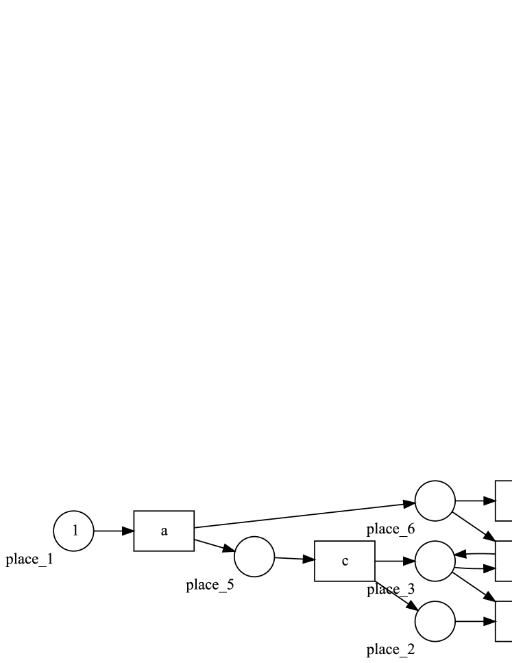
Figure 1: Result of ILP Based Discovery [44], containing a milestone pattern.

The model describes that activity $a$ is always executed first. After activity $a$ we are able to execute activity $c$ and $e$ in any order, i.e. they are in a parallel construct. However, after executing activity $c$ we are able to perform activity $b$ instead of $e$. However, this is only possible as long as we do not execute activity $d$, which we are able to execute after we have executed $c$. Finally we always execute activity $f$. In the model, the choice of executing activity $b$ instead of $e$ is influenced by the global state of the system. Such pattern is called a milestone pattern [6].

If we apply the aforementioned state-of-the-art discovery algorithms on these same data, we obtain the models depicted in Figure 2.

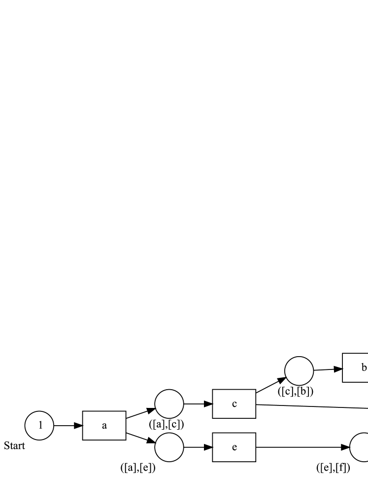
(a) $\alpha$-, $\alpha^{+}$-, $\alpha^{++}$-Miner [8, 32, 42].

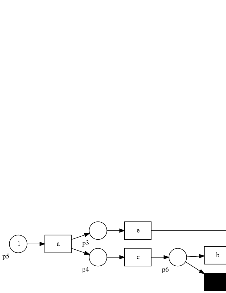
(b) $\alpha^{\sharp}$-Miner [43].

(c) Inductive-Miner [25].

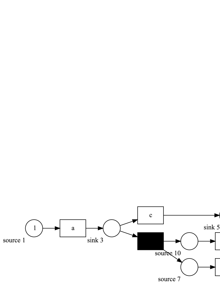
(d) Evolutionary Tree Miner [17].

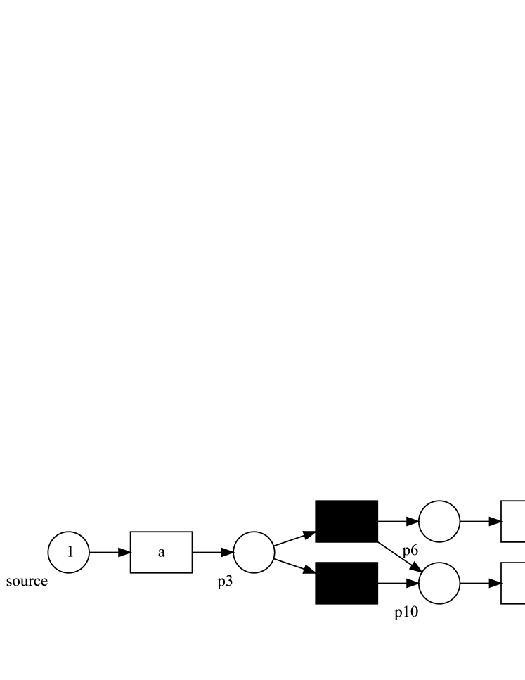
(e) Heuristics Miner [40, 41].

Figure 2: Results of several state-of-the-art discovery algorithms in the ProM Framework [38], when given sequences containing a milestone pattern.

None of the models adequately describes the milestone pattern. Some models do not even guarantee perfect replay-fitness, i.e. 2(a). Other models, such as the model in 2(c) have very low precision. The only model that actually describes the same behaviour is the model in 2(d). However, the model does not capture the milestone pattern, i.e. we need to analyse the behaviour of the model to derive the conclusion that it describes the behaviour of a milestone pattern.

As the example shows there is a clear incentive for process discovery algorithms based on (language-based) region theory. However, the state-of-the-art technique based on language-based region theory [44] has a number of deficiencies. It is not able to guarantee that the resulting Petri net is a workflow net, i.e. a Petri net with favourable graph-theoretical properties. For example, the Petri net in Figure 1 does not have a unique sink place. The Inductive Miner for example does guarantee to return (sound) workflow nets. Moreover, ILP-based process discovery greatly suffers from the presence of infrequent and/or exceptional behaviour. Assume we have an event log containing thousands of repetitions of the aforementioned sequences $\langle a\mathchar 44\relax c\mathchar 44\relax d\mathchar 44\relax e\mathchar 44\relax f\rangle$, $\langle a\mathchar 44\relax c\mathchar 44\relax b\mathchar 44\relax d\mathchar 44\relax f\rangle$, $\langle a\mathchar 44\relax c\mathchar 44\relax e\mathchar 44\relax d\mathchar 44\relax f\rangle$ and $\langle a\mathchar 44\relax e\mathchar 44\relax c\mathchar 44\relax d\mathchar 44\relax f\rangle$. If we inject just one exceptional sequence, e.g. $\langle a\mathchar 44\relax b\mathchar 44\relax c\mathchar 44\relax d\mathchar 44\relax f\rangle$, and apply the current state-of-art region-based discovery algorithm, we obtain the model depicted in Figure 3. Within the model, activity $b$ is now able to occur in parallel with activity $c$.

Figure 3: Result of applying ILP Based Discovery [44] on an event log containing a milestone pattern, and, infrequent (faulty) behaviour.

Thus, by adding one infrequent, exceptional sequence, the algorithm is no longer able to detect the milestone pattern.

In this paper we solve the two aforementioned issues. Firstly, we present an approach that guarantees to find relaxed sound workflow nets. Secondly, we present an effective integrated filtering technique that identifies and ignores infrequent and/or exceptional behaviour.

3 Related Work

We predominantly focus on related work in the area of region theory and its application to process discovery. We also focus on filtering techniques for process discovery. For a detailed overview of process discovery algorithms we refer to [2, 22, 39].

Region Theory and Petri Net Synthesis

Region theory is a solution to the Petri net synthesis problem [35]. The two terms are therefore often used interchangeably. The synthesis problem is to, given a behavioural system description, decide whether there exists a Petri net that allows for all behaviour described by the system description, and, at the same time minimizes additional behaviour. Initial work focused on solving the synthesis problem using transition systems as a system description [23, 24, 15], i.e. state-based region theory. A set of states within the transition system forms a region, which defines a place in the resulting Petri net. Region theory has also been applied using a prefix-closed language as a system description [10, 21], i.e. language-based region theory. Here, a region is an assignment of decision variables over the language’s alphabet, again defining a place in the resulting Petri net. Finally, language-based region theory has also been extended for labelled partial orders [28, 29, 14].

Process Discovery

In contrast to Petri net synthesis, process discovery aims at extracting a generalizing process model from an incomplete behavioural system description, i.e. an event log. Additionally, we typically need to abstract from infrequent behaviour in order to focus on the mainstream behaviour in the event log.

In [7] a process discovery approach is presented that transforms an event log into a transition system, after which state-based region theory is applied. Constructing the transition system is strongly parametrized, i.e. using different parameters yields different process discovery results. In [37] a similar approach is presented. The main contribution is a complexity reduction w.r.t. conventional region-based techniques.

In [13] a process discovery approach is presented based on language-based region theory. The method finds a minimal linear basis of a polyhedral cone of integer points, based on the event log. It guarantees perfect replay-fitness, whereas it does not maximize precision. The worst-case time complexity of the approach is exponential in the size of the event log. In [19] a process discovery algorithm is proposed based on the concept of numerical abstract domains. Based on the event log’s prefix-closure a convex polyhedron is approximated by means of calculating a convex hull. The convex hull is used to compute causalities within the input log by deducing a set of linear inequalities which represent places. In [44] a first design of a process discovery ILP-formulation is presented. An objective function is presented, which is generalized in [46], that allows for expressing a preference for finding certain Petri net places. The work also presents means to formulate ILP-constraints that help finding more advanced Petri net-types, e.g. Petri nets with reset- and inhibitor arcs.

All aforementioned techniques leverage the strict implications of region theory w.r.t. process discovery, i.e. precision maximization, poor generalization and poor simplicity, to some extend. However, the techniques still perform suboptimal. Since the techniques guarantee perfect replay-fitness, they tend to fail if exceptional behaviour is present in the event log, i.e. they produce models that are incorporating infrequent behaviour (outliers).

Filtering Infrequent Behaviour

Little work has been done regarding filtering of infrequent behaviour in context of process mining. The majority of work concerns unpublished/undocumented ad-hoc filtering implementations in the ProM framework [38].

In [20] an event log filtering technique is presented that filters on event level. Events within the event log are removed in case they do not fit an underlying, event log based, automaton. The technique can be used as a pre-processing step prior to invoking a discovery algorithm.

In [26] Leemans et al. show how to extend the Inductive Miner [25] with filtering capabilities to handle infrequent behaviour. The technique is tailored towards the internal working of the Inductive Miner algorithm and considers three different types of filters. Moreover, the technique exploits the inductive nature of the underlying algorithm, i.e. filters are applied on multiple levels.

4 Background

In this section we present basic notational conventions, event logs and workflow nets.

4.1 Bags, Sequences and Vectors

$X=\{e_{1}\mathchar 44\relax e_{2}\mathchar 44\relax...\mathchar 44\relax e_{n}\}$ denotes a set. $\mathcal{P}(X)$ denotes the power set of $X$. $\mathbb{N}$ denotes the set of positive integers including $0$ whereas $\mathbb{N}^{+}$ excludes $0$. $\mathbb{R}$ denotes the set of real numbers. A bag (bag) over $X$ is a function $B:X\rightarrow\mathbb{N}$ which we write as $[e_{1}^{v_{1}}\mathchar 44\relax e_{2}^{v_{2}}\mathchar 44\relax...\mathchar 44\relax e_{n}^{v_{n}}]$, where for $1\leq i\leq n$ we have $e_{i}\in X$, $v_{i}\in\mathbb{N}^{+}$ and $e_{i}^{v_{i}}\equiv B(e_{i})=v_{i}$. If for some element $e$, $B(e)=1$, we omit its superscript. An empty bag is denoted as $\emptyset$. Element inclusion applies to bags: if $e\in X$ and $B(e)>0$ then also $e\in B$. Set operations, i.e. $\uplus$, $\setminus$, $\cap$, extend to bags. The set of all bags over $X$ is denoted $\mathcal{B}(X)$.

A sequence $\sigma$ of length $k$ relates positions to elements $e\in X$, i.e. $\sigma:\{1\mathchar 44\relax 2\mathchar 44\relax...\mathchar 44\relax k\}\rightarrow X$. An empty sequence is denoted as $\epsilon$. We write every non-empty sequence as $\langle e_{1}\mathchar 44\relax e_{2}\mathchar 44\relax...\mathchar 44\relax e_{k}\rangle$. The set of all possible sequences over a set $X$ is denoted as $X^{*}$. We define concatenation of sequences $\sigma_{1}$ and $\sigma_{2}$ as $\sigma_{1}\cdot\sigma_{2}$, e.g., $\langle a\mathchar 44\relax b\rangle\cdot\langle c\mathchar 44\relax d\rangle=\langle a\mathchar 44\relax b\mathchar 44\relax c\mathchar 44\relax d\rangle$. Let $X^{\prime}\subseteq X$, we define $\downarrow_{X^{\prime}}\colon X^{*}\to X^{\prime*}$ recursively with $\downarrow_{X^{\prime}}(\epsilon)=\epsilon$ and $\downarrow_{X^{\prime}}(\langle x\rangle\cdot\sigma)=\langle x\rangle\cdot\downarrow_{X^{\prime}}(\sigma)$ if $x\in X^{\prime}$ and $\downarrow_{X^{\prime}}(\sigma)$ otherwise. We write $\sigma_{\downarrow_{X^{\prime}}}$ for $\downarrow_{X^{\prime}}(\sigma)$.

Given $X^{\prime}\subseteq X^{*}$, the prefix-closure of $X^{\prime}$ is: $\overline{X^{\prime}}=\{\sigma_{1}\in X^{*}|\exists_{\sigma_{2}\in X^{*}}(\sigma_{1}\cdot\sigma_{2}\in X^{\prime})\}$. We extend the notion of a prefix-closure on bags of sequences. Let $X^{\prime}\subseteq X^{*}$ and $B_{X^{\prime}}:X^{\prime}\rightarrow\mathbb{N}$ we define $\overline{B}_{X^{\prime}}:\overline{X^{\prime}}\rightarrow\mathbb{N}$, such that: $\overline{B}_{X^{\prime}}(\sigma)=B_{X}(\sigma)+\sum_{\sigma\cdot\langle e\rangle\in\overline{X^{\prime}}}\overline{B}_{X^{\prime}}(\sigma\cdot\langle e\rangle)$. For example, $B_{2}=[\langle a\mathchar 44\relax b\rangle^{5}\mathchar 44\relax\langle a\mathchar 44\relax c\rangle^{3}]$ yields $\overline{B}_{2}=[\epsilon^{8}\mathchar 44\relax\langle a\rangle^{8}\mathchar 44\relax\langle a\mathchar 44\relax b\rangle^{5}\mathchar 44\relax\langle a\mathchar 44\relax c\rangle^{3}]$.

Given set $X$ and a range of values $R\subseteq\mathbb{R}$. Vectors are denoted as $\vec{z}\in R^{|X|}$, where $\vec{z}(e)\in R$ and $e\in X$. We assume vectors to be column vectors. For vector multiplication we assume that vectors agree on their indices. Throughout the paper we assume a total ordering on sets of the same domain. Given $X=\{e_{1}\mathchar 44\relax e_{2}\mathchar 44\relax...\mathchar 44\relax e_{n}\}$ and $\vec{z}_{1}\mathchar 44\relax\vec{z}_{2}\in R^{|X|}$ we have $\vec{z}_{1}^{\intercal}\vec{z}_{2}=\sum_{i=1}^{n}\vec{z}_{1}(e_{i})\vec{z}_{2}(e_{i})$. A Parikh vector $\vec{p}$ represents the number of occurrences of an element within a sequence, i.e. $\vec{p}:X^{*}\rightarrow\mathbb{N}^{|X|}$ with $\vec{p}(\sigma)=(\#_{e_{1}}(\sigma)\mathchar 44\relax\#_{e_{2}}(\sigma)\mathchar 44\relax...\mathchar 44\relax\#_{e_{n}}(\sigma))$ where $\#_{e_{i}}(\sigma)=|\{i^{\prime}\in\{1\mathchar 44\relax 2\mathchar 44\relax...\mathchar 44\relax|\sigma|\}\mid\sigma(i^{\prime})=e_{i}\}|$.

4.2 Event Logs and Workflow Nets

In process discovery an event log acts as a main source of input and describes the actual execution of activities in context of a business process. An example event log, adopted from [2], is presented in Table 1.

Table 1: Fragment of a fictional event log (each line corresponds to an event).

Case-id	Activity	Resource	Time-stamp
…	…	…	…
1	register request ($a$)	John	2015-05-08:08.45
1	examine thoroughly ($b$)	Lucy	2015-05-08:09.13
2	register request ($a$)	John	2015-05-08:09.14
2	check ticket ($d$)	Pete	2015-05-08:10.11
1	check ticket ($d$)	Pete	2015-05-08:10.28
2	examine causally ($b$)	Rob	2015-05-08:10.43
1	decide ($e$)	Rob	2015-05-08:11.14
1	reject request ($h$)	Rob	2015-05-08:11.35
…	…	…	…

Consider all activities related to Case-id 1. John registers a request, after which Lucy examines it thoroughly. Pete checks the ticket after which Rob decides to reject the request. The execution of an activity in context of a business process is referred to as an event. A sequence of events, e.g. the sequence of events related to case 1, is referred to as a trace.

Let $\mathcal{A}$ denote the universe of all possible activities. An event log $L$ is a bag of sequences over $\mathcal{A}$, i.e., $L\in\mathcal{B}(\mathcal{A}^{*})$. Typically, there exists $A_{L}\subset\mathcal{A}$ of activities that are actually present in $L$. In some cases we refer to an event log as $L\in\mathcal{B}(A_{L}^{*})$. A sequence $\sigma\in L$ represents a trace. We write case 1 as trace $\langle$“register request”,“examine thoroughly”, “check ticket”, “decide”, “reject request”$\rangle$. In the remainder of the paper we use simple characters for activity names, e.g. we write case 1 as $\langle a\mathchar 44\relax b\mathchar 44\relax d\mathchar 44\relax e\mathchar 44\relax h\rangle$.

The goal within process discovery is to discover a process model based on an event log. In this paper we consider workflow nets (WF-nets) [1], based on Petri nets [34], to describe process models. We first introduce Petri nets and their execution semantics, after which we define workflow nets.

A Petri net is a bipartite graph consisting of a set of vertices called places and a set of vertices called transitions. Arcs connect places with transitions and vice versa. Additionally, transitions have a (possibly unobservable) label which describes the activity that the transition represents. A Petri net is a quadruple $N=(P\mathchar 44\relax T\mathchar 44\relax F\mathchar 44\relax\lambda)$, where $P$ is a set of places and $T$ is a set of transitions with $P\cap T=\emptyset$. $F$ denotes the flow relation of $N$, i.e., $F\subseteq(P\times T)\cup(T\times P)$. $\lambda$ denotes the label function, i.e. given a set of activities $\Lambda\subset\mathcal{A}$ and an unobservable activity $\tau\notin\Lambda$, it is defined as $\lambda\colon T\to\Lambda\cup\{\tau\}$. For a node $x\in P\cup T$, the pre-set of $x$ in $N$ is defined as $\bullet x=\{y\mid(y\mathchar 44\relax x)\in F\}$ and $x\bullet=\{y\mid(x\mathchar 44\relax y)\in F\}$ denotes the post-set of $x$. Graphically we represent places as circles and transitions as boxes. For every $(x\mathchar 44\relax y)\in F$ we draw an arc from $x$ to $y$. An example Petri net (which is also a WF-net) is depicted in Figure 4.

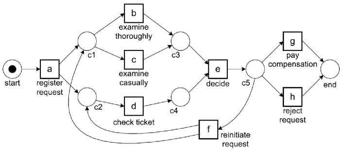
Figure 4: Example WF-net $W_{1}$, adopted from [2].

Observe that we have $\bullet d=\{c_{2}\}$, $d\bullet=\{c_{4}\}$ and $\lambda(d)=$“reject request”. The Petri net does not contain any silent transition.

The execution semantics of Petri nets are based on the concept of markings A marking $M$ is a bag of tokens, i.e. $M\in\mathcal{B}(P)$. Graphically, a place $p$’s marking is visualized by drawing $M(p)$ number of dots inside place $p$, e.g. place “start” in Figure 4. A marked Petri net is a $2$-tuple $(N\mathchar 44\relax M)$, where $M$ represents $N$’s marking. We let $M_{i}$ denote $N$’s initial marking. Transition $t\in T$ is enabled in marking $M$ if $\forall_{p\in\bullet t}(M(p)>0)$. Enabled transition $t$ in marking $M$, may fire, which results in new marking $M^{\prime}$. If $t$ fires, denoted as $(N\mathchar 44\relax M)\xrightarrow{t}(N\mathchar 44\relax M^{\prime})$, then for each $p\in P$ we have $M^{\prime}(p)=M(p)-1$ if $p\in\bullet t\setminus t\bullet$, $M^{\prime}(p)=M(p)+1$ if $p\in t\bullet\setminus\bullet t$, and, $M^{\prime}(p)=M(p)$ otherwise, e.g. in Figure 4 we have $(W_{1}\mathchar 44\relax[start])\xrightarrow{a}(W_{1}\mathchar 44\relax[c_{1}\mathchar 44\relax c_{2}])$. Given sequence $\sigma=\langle t_{1}\mathchar 44\relax t_{2}\mathchar 44\relax...\mathchar 44\relax t_{n}\rangle\in T^{*}$, $\sigma$ is a firing sequence of $(N\mathchar 44\relax M)$, written as $(N\mathchar 44\relax M)\xrightarrow[]{\sigma}\mathrel{\mkern-14.0mu}\rightarrow(N\mathchar 44\relax M^{\prime})$ if and only if for $n=|\sigma|$ there exist markings $M_{1}\mathchar 44\relax M_{2}\mathchar 44\relax...\mathchar 44\relax M_{n-1}$ such that $(N\mathchar 44\relax M)\xrightarrow{t_{1}}(N\mathchar 44\relax M_{1})$, $(N\mathchar 44\relax M_{1})\xrightarrow{t_{2}}(N\mathchar 44\relax M_{2})\mathchar 44\relax...\mathchar 44\relax(N\mathchar 44\relax M_{n-1})\xrightarrow{t_{n}}(N\mathchar 44\relax M^{\prime})$. We write $(N\mathchar 44\relax M)\xrightarrow[]{\sigma}\mathrel{\mkern-14.0mu}\rightarrow*$ if there exists a marking $M^{\prime}$ s.t. $(N\mathchar 44\relax M)\xrightarrow[]{\sigma}\mathrel{\mkern-14.0mu}\rightarrow(N\mathchar 44\relax M^{\prime})$. We write $(N\mathchar 44\relax M)\rightsquigarrow(N\mathchar 44\relax M^{\prime})$ if there exists $\sigma\in T^{*}$ s.t. $(N\mathchar 44\relax M)\xrightarrow[]{\sigma}\mathrel{\mkern-14.0mu}\rightarrow(N\mathchar 44\relax M^{\prime})$. We define $N$’s language as $\mathcal{L}(N\mathchar 44\relax M_{i})=\{\sigma\in T^{*}\mid M_{i}\xrightarrow[]{\sigma}\mathrel{\mkern-14.0mu}\rightarrow*\}$, i.e. $\mathcal{L}(N\mathchar 44\relax M_{i})$ is prefix-closed. We define $N$’s labelled language as $\mathcal{L}^{\Lambda}(N\mathchar 44\relax M_{i})=\{\sigma\in\Lambda^{*}\mid\exists_{\sigma^{\prime}\in T^{*}\mathchar 44\relax\sigma^{\prime\prime}\in(\Lambda\cup\{\tau\})^{*}}(\sigma^{\prime}\in\mathcal{L}_{(}N\mathchar 44\relax M_{i})\wedge|\sigma^{\prime}|=|\sigma^{\prime\prime}|\wedge\forall_{i\in\{1\mathchar 44\relax 2\mathchar 44\relax...\mathchar 44\relax|\sigma^{\prime}|\}}(\lambda(\sigma^{\prime}(i))=\sigma^{\prime\prime}(i))\wedge\sigma^{\prime\prime}_{\downarrow_{\Lambda}}=\sigma\}$. Given a final marking $M_{f}$, we define $N$’s execution language w.r.t. $M_{f}$ as $\mathcal{L}_{M_{f}}(N\mathchar 44\relax M_{i})=\{\sigma\in T^{*}\mid(N\mathchar 44\relax M_{i})\xrightarrow[]{\sigma}\mathrel{\mkern-14.0mu}\rightarrow(N\mathchar 44\relax M_{f})\}$. We define $N$’s labelled execution language as $\mathcal{L}^{\Lambda}_{M_{f}}(N\mathchar 44\relax M_{i})=\{\sigma\in\Lambda^{*}\mid\exists_{\sigma^{\prime}\in T^{*}\mathchar 44\relax\sigma^{\prime\prime}\in(\Lambda\cup\{\tau\})^{*}}(\sigma^{\prime}\in\mathcal{L}_{M_{f}}(N\mathchar 44\relax M_{i})\wedge|\sigma^{\prime}|=|\sigma^{\prime\prime}|\wedge\forall_{i\in\{1\mathchar 44\relax 2\mathchar 44\relax...\mathchar 44\relax|\sigma^{\prime}|\}}(\lambda(\sigma^{\prime}(i))=\sigma^{\prime\prime}(i))\wedge\sigma^{\prime\prime}_{\downarrow_{\Lambda}}=\sigma\}$

WF-nets extend Petri nets and require the existence of a unique source- and sink place which describe the start, respectively end, of a case. Moreover, each element within the WF-net needs to be on a path from the source to the sink place.

Definition 1 (Workflow net [1]).

Let $N=(P\mathchar 44\relax T\mathchar 44\relax F\mathchar 44\relax\lambda)$ be a Petri net. Let $p_{i}\mathchar 44\relax p_{o}\in P$ with $p_{i}\neq p_{o}$. Let $\Lambda\subset\mathcal{A}$ be a set of activities, let $\tau\notin\Lambda$ and let $\lambda\colon T\to\Lambda\cup\{\tau\}$. Tuple $W=(P\mathchar 44\relax T\mathchar 44\relax F\mathchar 44\relax p_{i}\mathchar 44\relax p_{o}\mathchar 44\relax\lambda)$ is a workflow net (WF-net) if and only if:

1. $\bullet p_{i}=\emptyset$

2. $p_{o}\bullet=\emptyset$

3. Each element $x\in P\cup T$ is on a path from $p_{i}$ to $p_{o}$.

The execution semantics defined for Petri nets can directly be applied on the elements $P$, $T$ and $F$ of $W=(P\mathchar 44\relax T\mathchar 44\relax F\mathchar 44\relax p_{i}\mathchar 44\relax p_{o}\mathchar 44\relax\lambda)$. Notation-wise we substitute $W$ for its underlying net structure $N=(P\mathchar 44\relax T\mathchar 44\relax F)$, e.g. $(W\mathchar 44\relax M)\xrightarrow{t}(W\mathchar 44\relax M^{\prime})$, $\mathcal{L}(W\mathchar 44\relax M_{i})$ etc. In context of WF-nets, we assume $M_{i}=[p_{i}]$ and $M_{f}=[p_{o}]$ unless mentioned otherwise.

We compute metrics such as replay-fitness and precision, as introduced in the introduction, based on an event log. Several behavioural quality metrics, that do not need any form of domain knowledge, exist for WF-nets. Several notions of soundness of WF-nets are defined [5]. For example, classical sound WF-nets are guaranteed to be free of livelocks, deadlocks, and other anomalies that can be detected automatically. In this paper we consider the weaker notion of relaxed soundness. Relaxed soundness requires that each transition is at some point enabled, and, after firing such transition we are able to eventually reach the final marking.

Definition 2 (Relaxed Soundness [5]).

Let $W=(P\mathchar 44\relax T\mathchar 44\relax F\mathchar 44\relax p_{i}\mathchar 44\relax p_{o}\mathchar 44\relax\lambda)$ be a WF-net. $W$ is relaxed sound if and only if: $\forall_{t\in T}(\exists_{M\mathchar 44\relax M^{\prime}\in\mathcal{B}(P)}((W\mathchar 44\relax[p_{i}])\rightsquigarrow(W\mathchar 44\relax M)\wedge(W\mathchar 44\relax M)\xrightarrow{t}(W\mathchar 44\relax M^{\prime})\wedge(W\mathchar 44\relax M^{\prime})\rightsquigarrow(W\mathchar 44\relax[p_{o}])))$.

Reconsider $W_{1}$ (Figure 4) and assume we are given an event log with one trace: $\langle a\mathchar 44\relax b\mathchar 44\relax d\mathchar 44\relax e\mathchar 44\relax h\rangle$. It is quite easy to see that $W_{1}$ is relaxed sound. Moreover, replay-fitness is perfect, i.e. $\langle a\mathchar 44\relax b\mathchar 44\relax d\mathchar 44\relax e\mathchar 44\relax h\rangle$ is in the WF-net’s labelled execution language. Precision is not perfect as the WF-net can produce a lot more traces than just $\langle a\mathchar 44\relax b\mathchar 44\relax d\mathchar 44\relax e\mathchar 44\relax h\rangle$.

5 Discovering Petri Net Places using Integer Linear Programming

In this section we show how to, given an event log as an input, discover multiple places of a Petri net using language based regions.

5.1 Regions

Conceptually, a region represents a place in a Petri net that, given the prefix-closure of an event log, does not block the execution of any sequence within the prefix-closure. We represent a region as an assignment of binary decision variables describing the incoming and outgoing arcs of its corresponding place, as well as its marking.

Definition 3 (Region).

Given an event log $L$ over a set of activities $A_{L}$. Let $m\in\{0\mathchar 44\relax 1\}$ and $\vec{x}\mathchar 44\relax\vec{y}\in\{0\mathchar 44\relax 1\}^{|A_{L}|}$. A triple $r=(m\mathchar 44\relax\vec{x}\mathchar 44\relax\vec{y})$ is a region if and only if:

$$\forall_{\sigma=\sigma^{\prime}\cdot\langle a\rangle\in\overline{L}}(m+\vec{p}(\sigma^{\prime})^{\intercal}\vec{x}-\vec{p}(\sigma)^{\intercal}\vec{y}\geq 0)$$ (5.1)

Variable $m$ indicates whether or not the region’s corresponding place contains a token, $\vec{x}$ denotes incoming arcs and $\vec{y}$ denotes outgoing arcs. Consider event log $L_{1}=[\langle a\mathchar 44\relax b\mathchar 44\relax d\mathchar 44\relax e\mathchar 44\relax g\rangle^{10}\mathchar 44\relax\langle a\mathchar 44\relax c\mathchar 44\relax d\mathchar 44\relax e\mathchar 44\relax f\mathchar 44\relax d\mathchar 44\relax b\mathchar 44\relax e\mathchar 44\relax g\rangle^{12}\mathchar 44\relax\langle a\mathchar 44\relax d\mathchar 44\relax c\mathchar 44\relax e\mathchar 44\relax h\rangle^{9}\mathchar 44\relax\langle a\mathchar 44\relax b\mathchar 44\relax d\mathchar 44\relax e\mathchar 44\relax f\mathchar 44\relax c\mathchar 44\relax d\mathchar 44\relax e\mathchar 44\relax g\rangle^{11}\mathchar 44\relax\langle a\mathchar 44\relax d\mathchar 44\relax c\mathchar 44\relax e\mathchar 44\relax f\mathchar 44\relax b\mathchar 44\relax d\mathchar 44\relax e\mathchar 44\relax h\rangle^{13}]$. In Table 2 we depict a part of the corresponding set of linear inequalities based on Definition 3.

Table 2: Linear inequalities corresponding to event log $L_{1}$ based on Equation 5.1.

$m-\vec{y}(a)\geq 0$	$\langle a\rangle$
$m+\vec{x}(a)-\vec{y}(a)-\vec{y}(b)\geq 0$	$\langle a\mathchar 44\relax b\rangle$
$m+\vec{x}(a)-\vec{y}(a)-\vec{y}(c)\geq 0$	$\langle a\mathchar 44\relax c\rangle$
$m+\vec{x}(a)+\vec{x}(b)-\vec{y}(a)-\vec{y}(b)-\vec{y}(d)\geq 0$	$\langle a\mathchar 44\relax b\mathchar 44\relax d\rangle$
$\vdots$	$\vdots$
$m+\vec{x}(a)+\vec{x}(b)+\vec{x}(c)+2\vec{x}(d)+2\vec{x}(e)+\vec{x}(f)-\vec{y}(a)-\vec{y}(b)-\vec{y}(c)-2\vec{y}(d)-2\vec{y}(e)-\vec{y}(f)-\vec{y}(h)\geq 0$	$\langle a\mathchar 44\relax d\mathchar 44\relax c\mathchar 44\relax e\mathchar 44\relax f\mathchar 44\relax b\mathchar 44\relax d\mathchar 44\relax e\mathchar 44\relax h\rangle$

For every non-empty sequence in $\overline{L_{1}}$, i.e. $\langle a\rangle$, $\langle a\mathchar 44\relax b\rangle$, …, $\langle a\mathchar 44\relax d\mathchar 44\relax c\mathchar 44\relax e\mathchar 44\relax f\mathchar 44\relax b\mathchar 44\relax d\mathchar 44\relax e\mathchar 44\relax h\rangle$ there is an associated linear inequality in terms of the variables $m$, $\vec{x}$ and $\vec{y}$. For example, $\langle a\rangle$ leads to $m-\vec{y}(a)$, $\langle a\mathchar 44\relax b\rangle$ leads to $m+\vec{x}(a)-\vec{y}(a)-\vec{y}(b)$ etc. Note that the inequalities abstract from the ordering of activities in traces, e.g. $\langle a\mathchar 44\relax c\mathchar 44\relax d\mathchar 44\relax e\rangle$ and $\langle a\mathchar 44\relax d\mathchar 44\relax c\mathchar 44\relax e\rangle$ both map to $m+\vec{x}(a)+\vec{x}(c)+\vec{x}(d)-\vec{y}(a)-\vec{y}(c)-\vec{y}(d)-\vec{y}(e)$.

A region $r$ is translated to a Petri net place $p$ as follows. Given a Petri net that has a unique transition $t_{a}$ for each $a\in A_{L}$ such that $\lambda(t_{a})=a$. If, for $a\in A_{L}$ $\vec{x}(a)=1$, we add $t_{a}$ to $\bullet p$. Symmetrically, if for $a\in A_{L}$ $\vec{y}(a)=1$, we add $t_{a}$ to $p\bullet$. Finally, if $m=1$, place $p$ is initially marked. Since translating a region to a place is deterministic, we are also able to translate a place to a region, e.g. place $c_{2}$ in Figure 4 corresponds to a region with $\vec{x}(a)=1$, $\vec{x}(f)=1$, $\vec{y}(d)=1$ and all other variables set to zero.

From a formal perspective, consider an event log $L$ over a set of activities $A_{L}$, a Petri net $N=(P\mathchar 44\relax T\mathchar 44\relax F\mathchar 44\relax\lambda)$ and marking $M_{i}$ s.t. $\overline{L}\subseteq\mathcal{L}^{\Lambda}(N\mathchar 44\relax M_{i})$. After adding a place, based on any possible region w.r.t. $L$, to $N$ (and updating $M_{i}$ if $m=1$) still $\overline{L}\subseteq\mathcal{L}^{\Lambda}(N\mathchar 44\relax M_{i})$ holds. However, adding the region potentially decreases the size of $\mathcal{L}^{\Lambda}(N\mathchar 44\relax M_{i})\setminus L$.

Triples $r_{\vec{0}}=(0\mathchar 44\relax\vec{0}\mathchar 44\relax\vec{0})$ and $r_{\vec{1}}=(1\mathchar 44\relax\vec{1}\mathchar 44\relax\vec{1})$ are always regions and hence are trivial regions. We let $R(L)$ denote the set of non-trivial regions based on event log $L$.

5.2 A Basic ILP Formulation

Set $R(L)$ represents a huge set of regions. However, when using $L_{1}$ as an input for process discovery, our goal is to find (a very similar WF-net to) the WF-net in Figure 4. Several regions exist in $R(L_{1})$ that are not a place in Figure 4. For example, a variable assignment with $\vec{x}(a)=1$ and $\vec{y}(e)=1$ (all other variables zero), i.e. representing a place connecting transitions $a$ and $e$, is a region. We therefore need means to search through the solution space to find regions that are of interest.

Firstly, we are only interested in minimal regions, i.e. regions that are not expressible as a non-negative linear combination of two other regions, because non-minimal regions correspond to implicit places [44]. Hence, when applying region-based techniques in terms of process discovery, we only search for minimal regions. Finding all minimal regions does however not suffice, e.g. the aforementioned region with $\vec{x}(a)=1$ and $\vec{y}(e)=1$ is minimal yet implicit. To this end we define an Integer Linear Programming (ILP) [36] formulation using the region definition as a constraint body [44]. ILP is a mathematical optimization problem defined over a set of integer variables. The objective and constraints of an ILP-problem are an expression in terms of the variables of linear form. Before introducing the basic ILP-formulation for the purpose of process discovery, we reformulate regions in terms of matrices.

Definition 4 (Region (Matrix Form)).

Given an event log $L$ over a set of activities $A_{L}$, let $m\in\{0\mathchar 44\relax 1\}$ and let $\vec{x}\mathchar 44\relax\vec{y}\in\{0\mathchar 44\relax 1\}^{|A_{L}|}$. Let $\mathbf{M}$ and $\mathbf{M}^{\prime}$ be two $|\overline{L}\setminus\{\epsilon\}|\times|A_{L}|$ matrices with $\mathbf{M}(\sigma\mathchar 44\relax a)=\vec{p}(\sigma)(a)$ and $\mathbf{M}^{\prime}(\sigma\mathchar 44\relax a)=\vec{p}(\sigma^{\prime})(a)$ (where $\sigma=\sigma^{\prime}\cdot\langle a^{\prime}\rangle\in\overline{L}$). Tuple $r=(m\mathchar 44\relax\vec{x}\mathchar 44\relax\vec{y})$ is a region if and only if:

$$m\vec{1}+\mathbf{M}^{\prime}\vec{x}-\mathbf{M}\vec{y}\geq\vec{0}$$ (5.2)

We additionally define matrix $\mathbf{M}_{L}$ which is an $|L|\times|A_{L}|$ matrix with $\mathbf{M}_{L}(\sigma\mathchar 44\relax a)=\vec{p}(\sigma)(a)$ for $\sigma\in L$, i.e., $\mathbf{M}_{L}$ is the equivalent of $\mathbf{M}$ for all traces in the event log. We define a general process discovery ILP-formulation that guarantees to find a non-trivial region with the additional property that the corresponding place is always empty after replaying each trace within the event log.

Definition 5 (Process Discovery ILP-formulation).

Given an event log $L$ over a set of activities $A_{L}$ and corresponding matrices $\mathbf{M}$, $\mathbf{M}^{\prime}$ and $\mathbf{M}_{L}$. Let $c_{m}\in\mathbb{R}$ and $\vec{c_{x}}\mathchar 44\relax\vec{c_{y}}\in\mathbb{R}^{|A_{L}|}$. The process discovery ILP-formulation, $ILP_{L}$, is defined as:

minimize		$z=c_{m}m+\vec{c_{x}}^{\intercal}\vec{x}+\vec{c_{y}}^{\intercal}\vec{y}$		objective function
such that		$m\vec{1}+\mathbf{M}^{\prime}\vec{x}-\mathbf{M}\vec{y}\geq\vec{0}$		theory of regions
and		$m\vec{1}+\mathbf{M}_{L}(\vec{x}-\vec{y})=\vec{0}$		corresp. place is empty after each trace
		$\vec{1}^{\intercal}\vec{x}+\vec{1}^{\intercal}\vec{y}\geq 1$		at least one arc connected
		$\vec{0}\leq\vec{x}\leq\vec{1}$		i.e. $\vec{x}\in\{0\mathchar 44\relax 1\}^{|A|}$
		$\vec{0}\leq\vec{y}\leq\vec{1}$		i.e. $\vec{y}\in\{0\mathchar 44\relax 1\}^{|A|}$
		$0\leq m\leq 1$		i.e. $m\in\{0\mathchar 44\relax 1\}$

Definition 5 acts as a basic formulation for process discovery using ILP. To actually use the formulation we need to instantiate $c_{m}$, $\vec{c_{x}}$ and $\vec{c_{y}}$, i.e. the objective coefficients, with meaningful values. By varying the actual values for the objective coefficients we are able to let the ILP favour different solutions. In [44] an objective function is proposed that minimizes the number of incoming arcs and maximizes the number of outgoing arcs to a place. In [46] the aforementioned objective function is extended such that it minimizes the time a token resides in the corresponding place. Both objective functions are expressible as a more general function which favours minimal regions [46]. In general we are able to use any objective function, as long as it favours minimal regions. Hence, in this paper we assume that one uses such objective function.

Using the basic formulation with some objective function instantiation only yields one, optimal, result. Hence we need a more structured approach for finding multiple Petri net places, using the ILP formulation presented as a basis.

5.3 Exploiting Causalities

We need to find multiple regions that together form places of a WF-net, in line with the behaviour present within the event log. One of the most suitable techniques to find multiple regions in a controlled, structured manner, is by exploiting causal relations present within an event log. A causal relation between activities $a$ and $b$ implies that activity $a$ causes $b$, i.e. $b$ is likely to follow (somewhere) after activity $a$.

Several approaches exist to compute causalities relations [22]. The $\alpha$-Miner [8] defines causal relation $a\to_{L}b$ from activity $a$ to activity $b$ if, within some event log $L$, we find traces of the form $\langle...\mathchar 44\relax a\mathchar 44\relax b\mathchar 44\relax...\rangle$ though we do not find traces of the form $\langle...\mathchar 44\relax b\mathchar 44\relax a\mathchar 44\relax...\rangle$. Within the Heuristics Miner [40, 41] this relation was further developed to take frequencies into account as well. Given these multiple definitions, we assume the existence of a causal relation oracle which, given an event log, produces a set of pairs $(a\mathchar 44\relax b)$ indicating that activity $a$ has a causal relation with (to) activity $b$.

Definition 6 (Causal relation oracle).

A causal relation oracle $\gamma_{c}$ maps a bag of traces to a set of activity pairs, i.e. $\gamma_{c}:\mathcal{B}(\mathcal{A}^{*})\to\mathcal{P}(\mathcal{A}\times\mathcal{A})$.

A causal oracle maps an event log onto its activities, i.e. $\gamma_{c}(L)\in\mathcal{P}(A_{L}\times A_{L})$. It defines a directed graph with $A_{L}$ as vertices and each pair $(a\mathchar 44\relax b)\in\gamma_{c}(L)$ as an arc between $a$ and $b$. Later we exploit this graph-based view, for now we refer to $\gamma_{c}(L)$ as a collection of pairs.

When adopting a causal-based ILP process discovery strategy, we try to find net places that represent a causality found in the event log. Given an event log $L$, for each pair $(a\mathchar 44\relax b)\in\gamma_{c}(L)$ we enrich the constraint body with three constraints: 1.) $m=0$, 2.) $\vec{x}(a)=1$ and 3.) $\vec{y}(b)=1$. The three constraints ensure that if we find a solution to the ILP it corresponds to a place which is not marked and connects transition $a$ to transition $b$. Given pair $(a\mathchar 44\relax b)\in\gamma_{c}(L)$ we denote the corresponding extended causality based ILP-formulation as $ILP_{(L\mathchar 44\relax a\to b)}$.

After solving $ILP_{(L\mathchar 44\relax a\to b)}$ for each $(a\mathchar 44\relax b)\in\gamma_{c}(L)$, we end up with a set of regions that we are able to transform into places in a resulting Petri net. Since we enforce $m=0$ for each causality, none of these places is initially marked. Moreover, due to constraints based on $m\vec{1}+\mathbf{M}_{L}(\vec{x}-\vec{y})=\vec{0}$, the resulting place is empty after replaying each trace in the input event log within the net. Since we additionally enforce $\vec{x}(a)=1\ \text{and}\ \vec{y}(b)=1$, if we find a solution to the ILP, the corresponding place has both input and output arcs and is not eligible for being a source/sink place. Hence, the approach as-is does not allow us to find WF-nets. In the next section we show that a simple pre-processing step performed on the event log, together with specific instances of $\gamma_{c}(L)$, allows us to discover WF-nets which are relaxed sound.

6 Discovering Relaxed Sound Workflow Nets

Reconsider example event log $L_{1}$, i.e. $L_{1}=[\langle a\mathchar 44\relax b\mathchar 44\relax d\mathchar 44\relax e\mathchar 44\relax g\rangle^{10}\mathchar 44\relax\langle a\mathchar 44\relax c\mathchar 44\relax d\mathchar 44\relax e\mathchar 44\relax f\mathchar 44\relax d\mathchar 44\relax b\mathchar 44\relax e\mathchar 44\relax g\rangle^{12}\mathchar 44\relax\langle a\mathchar 44\relax d\mathchar 44\relax c\mathchar 44\relax e\mathchar 44\relax h\rangle^{9}\mathchar 44\relax\langle a\mathchar 44\relax b\mathchar 44\relax d\mathchar 44\relax e\mathchar 44\relax f\mathchar 44\relax c\mathchar 44\relax d\mathchar 44\relax e\mathchar 44\relax g\rangle^{11}\mathchar 44\relax\langle a\mathchar 44\relax d\mathchar 44\relax c\mathchar 44\relax e\mathchar 44\relax f\mathchar 44\relax b\mathchar 44\relax d\mathchar 44\relax e\mathchar 44\relax h\rangle^{13}]$. Let $A_{f}\subseteq A_{L}$ denote the set of final activities, i.e. activities $a_{f}$ s.t. there exists a trace of the form $\langle...\mathchar 44\relax a_{f}\rangle$ in the event log. For example, for $L_{1}$, $A_{f}=\{g\mathchar 44\relax h\}$. After solving each $ILP_{L\mathchar 44\relax a\to b}$ instance based on $\gamma_{c}(L)$ and adding corresponding places, we know that when we exactly replay any trace from $L_{1}$, after firing $g$ or $h$, the net is empty. Since $g$ and $h$ never co-occur in a trace, it is trivial to add a sink place $p_{o}$, s.t. after replay each trace in $L_{1}$, $p_{o}$ is the only place marked, i.e. $\bullet p_{o}=\{f\mathchar 44\relax g\}$ and $p_{o}\bullet=\emptyset$ (place “end” in Figure 4). In general, such decision is not trivial. However, a trivial case for adding a sink $p_{o}$ is the case when there is only one end activity that uniquely occurs once, at the end of each trace, i.e. $A_{f}=\{a_{f}\}$ and there exists no trace of the form $\langle...\mathchar 44\relax a_{f}\mathchar 44\relax...\mathchar 44\relax a_{f}\rangle$. In such case we have $\bullet p_{o}=\{a_{f}\}$, $p_{o}\bullet=\emptyset$.

A similar rationale holds for adding a source place. We define a set $A_{s}$ that denotes the set of start activities, i.e. activities $a_{s}$ s.t. there exists a trace of the form $\langle a_{s}\mathchar 44\relax...\rangle$ in the event log. For each activity $a_{s}$ in $A_{s}$ we know that for some traces in the event log, these are the first ones to be executed. Thus, we know that the source place $p_{i}$ must connect, in some way, to the elements of $A_{s}$. Like in the case of final transitions, creating a source place is trivial when $A_{s}=\{a_{s}\}$ and there exists no trace of the form $\langle a_{s}\mathchar 44\relax...\mathchar 44\relax a_{s}\mathchar 44\relax...\rangle$, i.e. the start activity uniquely occurs once in each trace. In such case we create place $p_{i}$ with $\bullet p_{i}=\emptyset$, $p_{i}\bullet=\{a_{s}\}$.

In order to be able to find a source and a sink place, it suffices to guarantee that sets $A_{s}$ and $A_{f}$ are of size one and their elements always occur uniquely at the start, respectively, end of a trace. We formalize this idea through the notion of unique start/end event logs, after which we show that transforming an arbitrary event log to such unique start/end event log is trivial.

Definition 7 (Unique start/end event log).

Let $L$ be an event log over a set of activities $A_{L}$. $L$ is a Unique Start/End event Log (USE-Log) if there exist $a_{s}\mathchar 44\relax a_{f}\in A_{L}$ s.t. $a_{s}\neq a_{f}$, $\forall_{\sigma\in L}(\sigma(1)=a_{s}\wedge\forall_{i\in\{2\mathchar 44\relax 3\mathchar 44\relax...\mathchar 44\relax|\sigma|\}}(\sigma(i)\neq a_{s}))$ and $\forall_{\sigma\in L}(\sigma(|\sigma|)=a_{f}\wedge\forall_{i\in\{1\mathchar 44\relax 2\mathchar 44\relax...\mathchar 44\relax|\sigma|-1\}}(\sigma(i)\neq a_{f}))$.

Since the set of activities $A_{L}$ is finite, it is trivial to transform any event log to a USE-log. Assume we have an event log $L$ over $A_{L}$ that is not a USE-log. We generate two “fresh” activities $a_{s}\mathchar 44\relax a_{f}\in\mathcal{A}$ s.t. $a_{s}\mathchar 44\relax a_{f}\notin A_{L}$ and create a new event log $L^{\prime}$ over $A_{L}\cup\{a_{s}\mathchar 44\relax a_{f}\}$, by adding $\langle a_{s}\rangle\cdot\sigma\cdot\langle a_{f}\rangle$ to $L$ for each $\sigma\in L$. We let $\pi:\mathcal{B}(\mathcal{A}^{*})\to\mathcal{B}(\mathcal{A}^{*})$ denote such USE-transformation. We omit $a_{s}$ and $a_{f}$ from the domain of $\pi$ and assume that given some USE-transformation the two symbols are known.

Clearly, after applying a USE-transformation, finding a unique source and sink place is trivial. It also provides an additional advantage considering the ability to find WF-nets. In fact, an ILP instance $ILP_{L\mathchar 44\relax a\to b}$ always has a solution if $L$ is a USE-log. We provide a proof of this property in Lemma 1, after which we present an algorithm that, given specific instantiations of $\gamma_{c}$, discovers WF-nets.

Lemma 1 (A USE-Log based causality has a solution).

Let $L$ be an event log over a set of activities $A_{L}$. Let $\pi:\mathcal{B}(\mathcal{A}^{*})\to\mathcal{B}(\mathcal{A}^{*})$ denote a USE-transformation function and let $a_{s}$, $a_{f}$ denote the start and end activities. For every $(a\mathchar 44\relax b)\in\gamma_{c}(\pi(L))$ with $a\neq a_{f}$ and $b\neq a_{s}$, $ILP_{(\pi(L)\mathchar 44\relax a\to b)}$ has a solution.

Constructive.

We consider the case $a\neq a_{s}$ and $b\neq a_{f}$. We show that variable assignment $\vec{x}(a_{s})=\vec{x}(a)=\vec{x}(b)=\vec{y}(a)=\vec{y}(b)=\vec{y}(a_{f})=1$, all other variables $0$ (5(a)), adheres to all constraints of $ILP_{(\pi(L)\mathchar 44\relax a\to b)}$.

Consider constraints of the form $\forall_{\sigma=\sigma^{\prime}\cdot\langle a\rangle\in\overline{\pi(L)}}(m+\vec{p}(\sigma^{\prime})^{\intercal}\vec{x}-\vec{p}(\sigma)^{\intercal}\vec{y}\geq 0)$ ($m\vec{1}+\mathbf{M}^{\prime}\vec{x}-\mathbf{M}\vec{y}\geq\vec{0}$) and let $\sigma=\sigma^{\prime}\cdot\langle x\rangle\in\overline{\pi(L)}$.

Case I: $x\neq a\mathchar 44\relax x\neq b\mathchar 44\relax x\neq a_{f}$. Since $x\neq a_{f}$ we know $\vec{p}(\sigma)(a_{f})=0$. Moreover, since $x\neq a\mathchar 44\relax x\neq b$, we know that $\vec{p}(\sigma^{\prime})(a)=\vec{p}(\sigma)(a)$ and $\vec{p}(\sigma^{\prime})(b)=\vec{p}(\sigma)(b)$, and hence $\vec{p}(\sigma^{\prime})(a)\vec{x}(a)-\vec{p}(\sigma)(a)\vec{y}(a)=0$ and $\vec{p}(\sigma^{\prime})(b)\vec{x}(b)-\vec{p}(\sigma)(b)\vec{y}(b)=0$. Since $\vec{x}(a_{s})=1$ and $a_{s}$ occurs uniquely at the start of each trace, if $\sigma^{\prime}=\epsilon$ such constraint equals $0$, and, $1$ otherwise.

Case II: $x=a$. We know $\vec{p}(\sigma)(a_{f})=0$ and $\vec{p}(\sigma^{\prime})(b)=\vec{p}(\sigma)(b)$. Now $\vec{p}(\sigma^{\prime})(a)=\vec{p}(\sigma)(a)-1$ and thus $\vec{p}(\sigma^{\prime})(a)\vec{x}(a)-\vec{p}(\sigma)(a)\vec{y}(a)=-1$. Since $a_{s}\in\sigma^{\prime}$ we have $\vec{p}(\sigma^{\prime})(a_{s})\vec{x}(a_{s})=1$, and thus the constraint equals $0$.

Case III: $x=b$ Similar to Case II.

Case IV: $x=a_{f}$. We again have $\vec{p}(\sigma^{\prime})(a)=\vec{p}(\sigma)(a)$ and $\vec{p}(\sigma^{\prime})(b)=\vec{p}(\sigma)(b)$. Since $\vec{p}(\sigma)(a_{f})\vec{y}(a_{f})=\vec{p}(\sigma^{\prime})(a_{s})\vec{x}(a_{s})=1$, each constraint equals $0$.

The constraints of the form: $\vec{1}^{\intercal}\vec{x}+\vec{1}^{\intercal}\vec{y}\geq 1$, $\vec{0}\leq\vec{x}\leq\vec{1}$, $\vec{0}\leq\vec{y}\leq\vec{1}$ and $0\leq m\leq 1$ are trivially satisfied. From Case IV combined with $\vec{x}(a_{f})=0$ it follows that all constraints of the form $\forall_{\sigma\in\pi(L)}(m+\vec{p}(\sigma)^{\intercal}(\vec{x}-\vec{y})=0)$ ($m\vec{1}+\mathbf{M}_{L}(\vec{x}-\vec{y})=\vec{0}$) hold. Finally the assignment adheres to $m=0$, $\vec{x}(a)=1$ and $\vec{y}(b)=1$.

In case we have $a=a_{s}$ and $b\neq a_{f}$ the region $\vec{x}(a_{s})=\vec{x}(a)=\vec{y}(a)=\vec{y}(a_{f})=1$, all other variables $0$ (5(b)), is a solution. The proof is similar to the proof of the previous case.

In case we have $a\neq a_{s}$ and $b=a_{f}$ the region $\vec{x}(a_{s})=\vec{x}(b)=\vec{y}(b)=\vec{y}(a_{f})=1$, all other variables $0$ (5(b)), is a solution. Again the proof is similar to the proof in the first case.

Finally in case we have $a=a_{s}$ and $b=a_{f}$ the region $\vec{x}(a_{s})=\vec{y}(a_{f})=1$, all other variables $0$ (5(c)), is a solution. Again the proof is similar to the proof in the first case. ∎

(a) Solution in case $a\neq a_{s}$ and $b\neq a_{f}$.

(b) Solution in case $a=a_{s}$ and $b\neq a_{f}$ or $a\neq a_{s}$ and $b=a_{f}$.

(c) Solution in case $a=a_{s}$ and $b=a_{f}$.

Figure 5: Visualizations of trivial solutions to $ILP_{(\pi(L)\mathchar 44\relax a\to b)}$ in terms of Petri net places.

In Algorithm 1 we present an ILP-Based process discovery approach that uses a USE-log internally in order to find multiple Petri net places. For every $(a\mathchar 44\relax b)\in\gamma_{c}(\pi(L))$ with $a\neq a_{f}$ and $b\neq a_{s}$ it solves $ILP_{(\pi(L)\mathchar 44\relax a\to b)}$. Moreover, it finds a unique source and sink place.

input : $L\in\mathcal{B}(A_{L}^{*})$, $\gamma_{c}\colon\mathcal{B}(\mathcal{A}^{*})\to\mathcal{P}(\mathcal{A}\times\mathcal{A})$

output : $W=(P\mathchar 44\relax T\mathchar 44\relax F\mathchar 44\relax p_{i}\mathchar 44\relax p_{o}\mathchar 44\relax\lambda)$

begin

      1 $P\mathchar 44\relax T\mathchar 44\relax F\leftarrow\emptyset$;

      2 let $a_{s}\mathchar 44\relax a_{f}\notin A_{L}$;

      3 $T\leftarrow\{t_{a}\mid a\in A_{L}\cup\{a_{s}\mathchar 44\relax a_{f}\}\}$;

      4 foreach $(a\mathchar 44\relax b)\in\gamma_{c}(\pi(L))$ do

            5 $(m\mathchar 44\relax\vec{x}\mathchar 44\relax\vec{y})\leftarrow$ solution to $ILP_{(\pi(L)\mathchar 44\relax a\to b)}$;

            6 let $p_{(a\mathchar 44\relax b)}\notin P$;

            7 $P\leftarrow P\cup p_{(a\mathchar 44\relax b)}$;

            8 foreach $a^{\prime}\in A_{L}\cup\{a_{s}\mathchar 44\relax a_{f}\}$ do

                  9 if $\vec{x}(a^{\prime})=1$ then

                        10 $F\leftarrow F\cup\{(t_{a^{\prime}}\mathchar 44\relax p_{(a\mathchar 44\relax b)}\}$;

                        

                  11if $\vec{y}(a^{\prime})=1$ then

                        12 $F\leftarrow F\cup\{(p_{(a\mathchar 44\relax b)}\mathchar 44\relax t_{a^{\prime}})\}$;

                        

                  

            

      13let $p_{i}\mathchar 44\relax p_{o}\notin P$;

      14 $P\leftarrow P\cup\{p_{i}\mathchar 44\relax p_{o}\}$;

      15 $F\leftarrow F\cup\{(p_{i}\mathchar 44\relax t_{a_{s}})\}$;

      16 $F\leftarrow F\cup\{(t_{a_{f}}\mathchar 44\relax p_{o})\}$;

      17 let $\lambda\colon T\to A\cup\{\tau\}$;

      18 foreach $a\in A_{L}$ do

            19 $\lambda(t_{a})\leftarrow a$ ;

            

      20$\lambda(t_{a_{s}})\mathchar 44\relax\lambda(t_{a_{f}})\leftarrow\tau$;

      21 $\mathbf{return}$ $(P\mathchar 44\relax T\mathchar 44\relax F\mathchar 44\relax p_{i}\mathchar 44\relax p_{o}\mathchar 44\relax\lambda)$;

      

Algorithm 1 ILP-Based Process Discovery

The algorithm constructs an initially empty Petri net $N=(P\mathchar 44\relax T\mathchar 44\relax F)$. Subsequently for each $a\in A_{L}\cup\{a_{s}\mathchar 44\relax a_{f}\}$ a transition $t_{a}$ is added to $T$. For each causal pair in the USE-variant of input event log $L$, a place $p_{(a\mathchar 44\relax b)}$ is discovered by solving $ILP_{(\pi(L)\mathchar 44\relax a\to b)}$ after which $P$ and $F$ are updated accordingly. The algorithm adds an initial place $p_{i}$ and connects it to $t_{a_{s}}$ and similarly creates sink place $p_{o}$ which is connected to $t_{a_{f}}$. For transition $t_{a}$ related to $a\in A_{L}$, we have $\lambda(t_{a})=a$, whereas $\lambda(t_{a_{s}})=\lambda(t_{a_{f}})=\tau$.

The algorithm is guaranteed to always find a solution to $ILP_{(\pi(L)\mathchar 44\relax a\to b)}$, hence for each causal relation a place is found. Additionally, a unique source and sink place are constructed. However, the algorithm does not guarantee that we find a connected component, i.e. requirement 3 of Definition 1. In fact, the nature of $\gamma_{c}$ determines whether or not we discover a WF-net. In Theorem 1 we characterize this nature and prove, by exploiting Lemma 1, that we are able to discover WF-nets.

Theorem 1 (There exist sufficient conditions for finding WF-nets).

Let $L$ be an event log over a set of activities $A_{L}$. Let $\pi:\mathcal{B}(\mathcal{A}^{*})\to\mathcal{B}(\mathcal{A}^{*})$ denote a USE-transformation function. Let $a_{s}\mathchar 44\relax a_{f}$ denote the unique start- and end activity of $\pi(L)$. Let $\gamma_{c}:\mathcal{B}(\mathcal{A}^{*})\to\mathcal{P}(\mathcal{A}\times\mathcal{A})$ be a causal oracle and consider $\gamma_{c}(\pi(L))$ as a directed graph. If each $a\in A_{L}$ is on a path from $a_{s}$ to $a_{f}$ in $\gamma_{c}(\pi(L))$, and there is no path from $a_{s}$ to itself, nor a path from $a_{f}$ to itself, then $\texttt{ILP-Based Process Discovery}(L\mathchar 44\relax\gamma_{c})$ returns a WF-net.

On the structure of $\gamma_{c}(\pi(L))$.

By the requirements on $\gamma_{c}(\pi(L))$ and Lemma 1, we know that for each $(a\mathchar 44\relax b)\in\gamma_{c}(\pi(L))$ a corresponding place will be found that has a transition labelled with $a$ as an input and a transition labelled $b$ as an output. Hence every path in $\gamma_{c}(\pi(L))$ corresponds to a path in the resulting net and as a consequence, every transition is on a path from $a_{s}$ to $a_{f}$. As every place that is added has input transition ($\vec{x}(a)=1$) and an output transition ($\vec{y}(b)=1$), every place is also on a path from $a_{s}$ to $a_{f}$. By construction this then also holds from $p_{i}$ to $p_{o}$. ∎

Theorem 1 proves that if we use a causal structure that, when interpreting it as a graph, has the property that each $a\in A_{L}$ is on a path from $a_{s}$ to $a_{f}$, the result of $\texttt{ILP-Based Process Discovery}(L\mathchar 44\relax\gamma_{c})$ is a WF-net. Although this seems a rather strict property of the causal structure, there exists a specific causal graph definition that guarantees this property [41]. Hence we are able to use this definition as an instantiation for $\gamma_{c}$.

Theorem 1 does not provide any behavioural guarantees, i.e. a WF-net is a purely graph-theoretical property. Recall that the premise of a region is that it does not block the execution of any sequence within the prefix-closure of an event log. Intuitively we deduce that we are therefore able to fire each transition in the WF-net at least once. Moreover, since we know that $a_{f}$ is the final transition of each sequence in $\pi(L)$, and after firing the transition each place based on any $ILP_{\pi(L)\mathchar 44\relax a\to b}$ is empty, we know that we are able to mark $p_{o}$. These two observations hint on the fact that the WF-net is relaxed sound, which we prove in Theorem 2

Theorem 2.

Let $L$ be an event log over a set of activities $A_{L}$. Let $\pi:\mathcal{B}(\mathcal{A}^{*})\to\mathcal{B}(\mathcal{A}^{*})$ denote a USE-transformation function and let $a_{s}\mathchar 44\relax a_{f}$ denote the unique start- and end activity of $\pi(L)$. Let $\gamma_{c}:\mathcal{B}(\mathcal{A}^{*})\to\mathcal{P}(\mathcal{A}\times\mathcal{A})$ be a causal oracle. Let $W=(P\mathchar 44\relax T\mathchar 44\relax F\mathchar 44\relax p_{i}\mathchar 44\relax p_{o}\mathchar 44\relax\lambda)=\texttt{ILP-Based Process Discovery}(L\mathchar 44\relax\gamma_{c})$. If $W$ is a WF-net, then $W$ is relaxed sound.

By construction of traces in the event log.

Recall that $W$ is relaxed sound if and only if: $\forall_{t\in T}(\exists_{M\mathchar 44\relax M^{\prime}\in\mathcal{B}(P)}((W\mathchar 44\relax[p_{i}])\rightsquigarrow(W\mathchar 44\relax M)\wedge(W\mathchar 44\relax M)\xrightarrow{t}(W\mathchar 44\relax M^{\prime})\wedge(W\mathchar 44\relax M^{\prime})\rightsquigarrow(W\mathchar 44\relax[p_{o}])))$.

Observe that $t_{a_{s}}$ is trivially enabled in $M_{i}=[p_{i}]$ since $\bullet t_{a_{s}}=\{p_{i}\}$. Consider arbitrary $t\in T\setminus\{t_{a_{s}}\mathchar 44\relax t_{a_{f}}\}$. We know $\exists_{\sigma\in\pi(L)}(\sigma=\langle a_{s}\rangle\cdot\sigma^{\prime}\cdot\langle\lambda(t)\rangle\cdot\sigma^{\prime\prime}\cdot\langle a_{f}\rangle)$.

Let $\langle t^{\prime}_{1}\mathchar 44\relax t^{\prime}_{2}\mathchar 44\relax...\mathchar 44\relax t^{\prime}_{n}\rangle$ s.t. $\langle\lambda(t^{\prime}_{1})\mathchar 44\relax\lambda(t^{\prime}_{2})\mathchar 44\relax...\mathchar 44\relax\lambda(t^{\prime}_{n})\rangle=\sigma^{\prime}$. The fact that each place $p\in P\setminus\{p_{i}\mathchar 44\relax p_{o}\}$ corresponds to a region yields that we may deduce $[p_{i}]\xrightarrow{t_{a_{s}}}M^{\prime}_{1}$,$M^{\prime}_{1}\xrightarrow{t^{\prime}_{1}}M^{\prime}_{2}$,…,$M^{\prime}_{n}\xrightarrow{t^{\prime}_{n}}M^{\prime}$ s.t. $M^{\prime}\supseteq\bullet t$ (if there exists $p\in\bullet t$ s.t. $M^{\prime}(p)=0$, then $p$ does not correspond to a region). Hence for any $t\in T\setminus\{t_{a_{s}}\mathchar 44\relax t_{a_{f}}\}$ there exists a marking reachable from $[p_{i}]$ that enables $t$.

Now let $\langle t^{\prime\prime}_{1}\mathchar 44\relax t^{\prime\prime}_{2}\mathchar 44\relax...\mathchar 44\relax t^{\prime\prime}_{n}\rangle$ s.t. $\langle\lambda(t^{\prime\prime}_{1})\mathchar 44\relax\lambda(t^{\prime\prime}_{2})\mathchar 44\relax...\mathchar 44\relax\lambda(t^{\prime\prime}_{n})\rangle=\sigma^{\prime\prime}$. Note that also, again by the fact that each place $p\in P\setminus\{p_{i}\mathchar 44\relax p_{o}\}$ corresponds to a region, we may deduce $M^{\prime}\xrightarrow{t^{\prime\prime}_{1}}M^{\prime\prime}_{1}$, $M^{\prime\prime}_{1}\xrightarrow{t^{\prime\prime}_{2}}M^{\prime\prime}_{2}$,…,$M^{\prime\prime}_{n-1}\xrightarrow{t^{\prime\prime}_{n}}M^{\prime\prime}_{n}$. Clearly we have $M^{\prime\prime}_{n}\xrightarrow{t_{a_{f}}}M_{f}$ with $M_{f}(p_{o})=1$ since $t_{a_{f}}\bullet=\{p_{o}\}$, and this is the first time we fire $t_{a_{f}}$, i.e., $a_{f}\notin\langle a_{s}\rangle\cdot\sigma^{\prime}\cdot\langle\lambda(t)\rangle\cdot\sigma^{\prime\prime}$. Clearly $M_{f}(p_{i})=0$ and because of constraints of the form $m\vec{1}+\mathbf{M}_{L}(\vec{x}-\vec{y})=\vec{0}$ we have $\forall_{p\in P\setminus\{p_{i}\mathchar 44\relax p_{o}\}}(M_{f}(p)=0)$. Hence $M_{f}=[p_{o}]$ and thus after firing $t$ there exists a firing sequence that leads to marking $[p_{o}]$ which proves $W$ is relaxed sound. ∎

We have shown that with a few pre- and post-processing steps and a specific class of causal structures we are able to guarantee to find WF-nets that are relaxed sound. These results are interesting since several process mining techniques require WF-nets as an input. The ILP problems solved still require their solutions to allow for all possible behaviour in the event log. As a result, the algorithm incorporates all infrequent exceptional behaviour and still results in over-fitting complex WF-nets. Hence, in the upcoming section we show how to efficiently prune the ILP constraint body to identify and eliminate infrequent exceptional behaviour.

7 Dealing with Infrequent Behaviour

In this section we present an efficient pruning technique that identifies and eliminates constraints related to infrequent exceptional behaviour. We first present the impact of infrequent exceptional behaviour after which we present the pruning technique.

7.1 The Impact of Infrequent Exceptional Behaviour

In Section 2 we already indicated the impact of infrequent behaviour on the results of ILP-based process discovery. In this section we highlight the main cause of ILP-based discovery’s inability to handle infrequent behaviour and we devise a filtering mechanism that exploits the nature of the underlying body of constraints.

Let us again reconsider example event log $L_{1}$, i.e., $L_{1}=[\langle a\mathchar 44\relax b\mathchar 44\relax d\mathchar 44\relax e\mathchar 44\relax g\rangle^{10}\mathchar 44\relax\langle a\mathchar 44\relax c\mathchar 44\relax d\mathchar 44\relax e\mathchar 44\relax f\mathchar 44\relax d\mathchar 44\relax b\mathchar 44\relax e\mathchar 44\relax g\rangle^{12}\mathchar 44\relax\langle a\mathchar 44\relax d\mathchar 44\relax c\mathchar 44\relax e\mathchar 44\relax h\rangle^{9}\mathchar 44\relax\langle a\mathchar 44\relax b\mathchar 44\relax d\mathchar 44\relax e\mathchar 44\relax f\mathchar 44\relax c\mathchar 44\relax d\mathchar 44\relax e\mathchar 44\relax g\rangle^{11}\mathchar 44\relax\langle a\mathchar 44\relax d\mathchar 44\relax c\mathchar 44\relax e\mathchar 44\relax f\mathchar 44\relax b\mathchar 44\relax d\mathchar 44\relax e\mathchar 44\relax h\rangle^{13}]$. Using an implementation of Algorithm 1 in ProM [38], with a suitable causal structure $\gamma_{c}$, we find the WF-net depicted in 6(a).

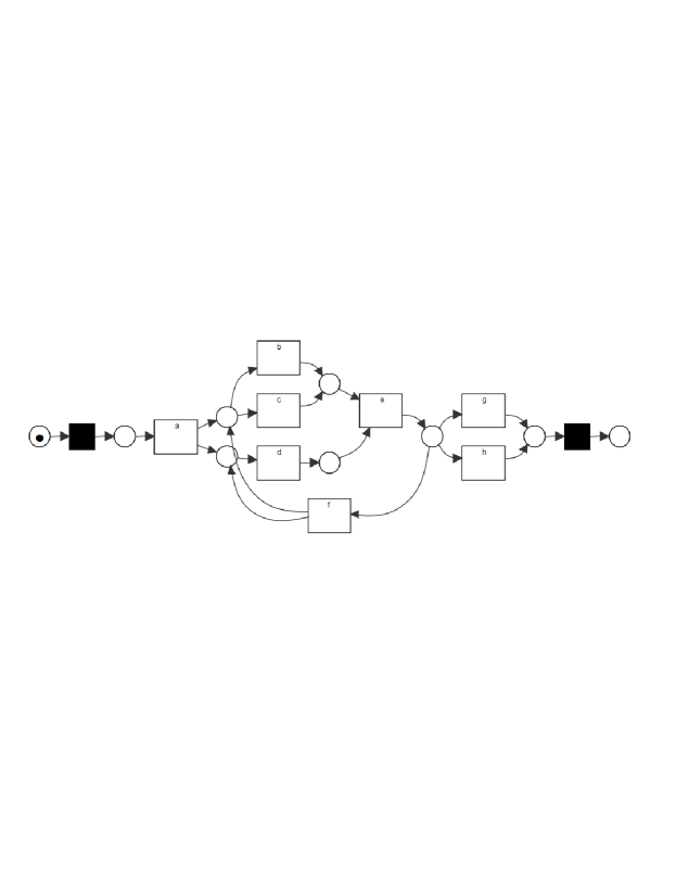
(a) Result based on event log $L_{1}$

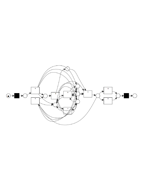
(b) Result based on event log $L^{\prime}_{1}$

Figure 6: Results of applying Algorithm 1 (HybridILPMiner package in the ProM Framework [38]) based on $L_{1}$ and $L^{\prime}_{1}$.

The WF-net describes the same behaviour as the model presented in Figure 4 and has perfect replay-fitness w.r.t. $L_{1}$. However, if we create event log $L^{\prime}$ by simply adding one instance of the trace $\langle a\mathchar 44\relax b\mathchar 44\relax c\mathchar 44\relax d\mathchar 44\relax e\mathchar 44\relax g\rangle$, we obtain the result depicted in 6(b). Due to one exceptional trace, the model allows us, after executing $a$ or $f$ to execute an arbitrary number of $b$- and $c$-labelled transitions. This is undesirable since precision of the resulting process model drops significantly. Thus, the addition of one exceptional trace results in a less comprehensible WF-net and reduces the precision of the resulting WF-net.

When analysing the two models we observe that they share some equal places, e.g. both models have a place $p_{(\{a\mathchar 44\relax f\}\mathchar 44\relax\{d\})}$ with $\bullet p_{(\{a\mathchar 44\relax f\}\mathchar 44\relax\{d\})}=\{a\mathchar 44\relax f\}$ and $p_{(\{a\mathchar 44\relax f\}\mathchar 44\relax\{d\})}\bullet=\{d\}$. However, the two places $p_{(\{a\mathchar 44\relax f\}\mathchar 44\relax\{b\mathchar 44\relax c\})}$ with $\bullet p_{(\{a\mathchar 44\relax f\}\mathchar 44\relax\{b\mathchar 44\relax c\})}=\{a\mathchar 44\relax f\}$ and $p_{(\{a\mathchar 44\relax f\}\mathchar 44\relax\{b\mathchar 44\relax c\})}\bullet=\{b\mathchar 44\relax c\}$ and $p_{(\{b\mathchar 44\relax c\}\mathchar 44\relax\{e\})}$ with $\bullet p_{(\{b\mathchar 44\relax c\}\mathchar 44\relax\{e\})}=\{b\mathchar 44\relax c\}$ and $p_{(\{b\mathchar 44\relax c\}\mathchar 44\relax\{e\})}\bullet=\{e\}$ in 6(a), are not present in 6(b). These are “replaced” by the less desirable places containing self-loops in 6(b). This is caused by the fact that $L^{\prime}_{1}$ contains all traces present in $L_{1}$, combined with the additional constraints depicted in Table 3.

For place $p_{(\{a\mathchar 44\relax f\}\mathchar 44\relax\{b\mathchar 44\relax c\})}$ in 6(a) we define a corresponding tuple $r=(m\mathchar 44\relax\vec{x}\mathchar 44\relax\vec{y})$ with $\vec{x}(a)=1$, $\vec{x}(f)=1$, $\vec{y}(b)=1$ and $\vec{y}(c)=1$ (all other variables 0). The additional constraints in Table 3 all evaluate to $-1$ for $r$, e.g. constraint $m+\vec{x}(a_{s})+\vec{x}(a)+\vec{x}(b)-\vec{y}(a_{s})-\vec{y}(a)-\vec{y}(b)-\vec{y}(c)$ evaluates to $0+0+1+0-0-0-1-1=-1$. In case of place $p_{(\{b\mathchar 44\relax c\}\mathchar 44\relax\{e\})}$ we observe that the corresponding tuple $r=(m\mathchar 44\relax\vec{x}\mathchar 44\relax\vec{y})$ with $\vec{x}(b)=1$, $\vec{x}(c)=1$ and $\vec{y}(e)=1$, yields a value of $1$ for all constraints generated by trace $\langle a\mathchar 44\relax b\mathchar 44\relax c\mathchar 44\relax d\mathchar 44\relax e\mathchar 44\relax g\rangle$. For all constraints having a “$\geq 0$ right hand side” this is valid, however, for constraint $m+\vec{x}(a_{s})+\vec{x}(a)+\vec{x}(b)+\vec{x}(c)+\vec{x}(d)+\vec{x}(e)+\vec{x}(g)+\vec{x}(a_{f})-\vec{y}(a_{s})-\vec{y}(a)-\vec{y}(b)-\vec{y}(c)-\vec{y}(d)-\vec{y}(e)-\vec{y}(g)-\vec{y}(a_{f})=0$ this is not valid.

Table 3: Some of the newly added constraints based on trace $\langle a\mathchar 44\relax b\mathchar 44\relax c\mathchar 44\relax d\mathchar 44\relax e\mathchar 44\relax g\rangle$ in event log $L^{\prime}_{1}$, starting from prefix $\langle a\mathchar 44\relax b\mathchar 44\relax c\rangle$ which is not present in $\overline{L_{1}}$.

$m+\vec{x}(a_{s})+\vec{x}(a)+\vec{x}(b)-\vec{y}(a_{s})-\vec{y}(a)-\vec{y}(b)-\vec{y}(c)\geq 0$

$m+\vec{x}(a_{s})+\vec{x}(a)+\vec{x}(b)+\vec{x}(c)-\vec{y}(a_{s})-\vec{y}(a)-\vec{y}(b)-\vec{y}(c)-\vec{y}(d)\geq 0$

$\vdots$

$m+\vec{x}(a_{s})+\vec{x}(a)+\vec{x}(b)+\vec{x}(c)+\vec{x}(d)+\vec{x}(e)+\vec{x}(g)-\vec{y}(a_{s})-\vec{y}(a)-\vec{y}(b)-\vec{y}(c)-\vec{y}(d)-\vec{y}(e)-\vec{y}(g)-\vec{y}(a_{f})\geq 0$

$m+\vec{x}(a_{s})+\vec{x}(a)+\vec{x}(b)+\vec{x}(c)+\vec{x}(d)+\vec{x}(e)+\vec{x}(g)+\vec{x}(a_{f})-\vec{y}(a_{s})-\vec{y}(a)-\vec{y}(b)-\vec{y}(c)-\vec{y}(d)-\vec{y}(e)-\vec{y}(g)-\vec{y}(a_{f})=0$

The example shows that the addition of $\langle a\mathchar 44\relax b\mathchar 44\relax c\mathchar 44\relax d\mathchar 44\relax e\mathchar 44\relax g\rangle$ yields constraints that invalidate places $p_{(\{a\mathchar 44\relax f\}\mathchar 44\relax\{b\mathchar 44\relax c\})}$ and $p_{(\{b\mathchar 44\relax c\}\mathchar 44\relax\{e\})}$. As a result the WF-net based on event log $L^{\prime}_{1}$ contains places with self-loops on both $b$ and $c$ which greatly reduces its precision and simplicity. Due to the relative infrequency of trace $\langle a\mathchar 44\relax b\mathchar 44\relax c\mathchar 44\relax d\mathchar 44\relax e\mathchar 44\relax g\rangle$ it is arguably acceptable to trade-off the perfect replay-fitness guarantee of ILP-Based process discovery and return the WF-net of 6(a), given $L^{\prime}_{1}$. Hence, we need filtering techniques and/or trace clustering techniques in order to remove exceptional behaviour. However, apart from simple pre-processing, we aim at adapting the ILP-based process discovery approach itself to be able to cope with infrequent behaviour.

By manipulating the constraint body such that it no longer allows for all behaviour present in the input event log, we are able to deal with infrequent behaviour within event logs. Given the problems that arise because of the presence of exceptional traces, a natural next step is to leave out the constraints related to the problematic traces. An advantage of filtering the constraint body is the fact that the constraints are based on the prefix-closure of the event log. Thus, even if all traces are unique yet they do share prefixes, we are able to filter. Additionally, leaving out constraints decreases the size of the ILP’s constraint body, which has a potential positive effect on the time needed to solve an ILP. We devise a graph-based filtering technique, i.e., sequence encoding filtering, that allows us to prune constraints based on trace frequency information.

7.2 Sequence Encoding Graphs

As a first step towards sequence encoding filtering we define the relationship between sequences and constraints. We do this in terms of sequence encodings. A sequence encoding is a vector-based representation of a sequence in terms of region theory, i.e., representing the sequence’s corresponding constraint.

Definition 8 (Sequence encoding).

Given a set of activities $A=\{a_{1}\mathchar 44\relax a_{2}\mathchar 44\relax...\mathchar 44\relax a_{n}\}$. $\vec{\phi}:A^{*}\rightarrow\mathbb{N}^{2|A|+1}$ denotes the sequence encoding function mapping every $\sigma\in A^{*}$ to a $2\cdot|A|+1$-sized vector. We define $\vec{\phi}$ as:

$$\vec{\phi}(\sigma^{\prime}\cdot\langle a\rangle)=\begin{pmatrix}1\\ \vec{p}(\sigma^{\prime})\\ -\vec{p}(\sigma^{\prime}\cdot\langle a\rangle)\end{pmatrix}$$

As an example of a sequence encoding vector consider sequence $\langle a_{s}\mathchar 44\relax a\mathchar 44\relax b\rangle$ originating from $\overline{\pi(L^{\prime}_{1})}$, for which we have $\vec{\phi}(\langle a_{s}\mathchar 44\relax a\mathchar 44\relax b\rangle)^{\intercal}=(1\mathchar 44\relax 1\mathchar 44\relax 1\mathchar 44\relax 0\mathchar 44\relax 0\mathchar 44\relax 0\mathchar 44\relax 0\mathchar 44\relax 0\mathchar 44\relax 0\mathchar 44\relax 0\mathchar 44\relax 0\mathchar 44\relax-1\mathchar 44\relax-1\mathchar 44\relax-1\mathchar 44\relax 0\mathchar 44\relax 0\mathchar 44\relax 0\mathchar 44\relax 0\mathchar 44\relax 0\mathchar 44\relax 0\mathchar 44\relax 0)$. Sequence encoding vectors directly correspond to region theory based constraints, e.g. if we are given $m\in\{0\mathchar 44\relax 1\}$ and $\vec{x}\mathchar 44\relax\vec{y}\in\{0\mathchar 44\relax 1\}^{|A|}$ and create a vector $\vec{r}$ where $\vec{r}(1)=m$, $\vec{r}(2)=\vec{x}(a_{s})$, $\vec{r}(3)=\vec{x}(a)$, …, $\vec{r}(10)=\vec{x}(h)$, $\vec{r}(11)=\vec{x}(a_{f})$, $\vec{r}(12)=\vec{y}(a_{f})$, …, $\vec{r}(21)=\vec{y}(a_{f})$, then $\vec{\phi}(\langle a_{s}\mathchar 44\relax a\mathchar 44\relax b\rangle)^{\intercal}\vec{r}=m+\vec{x}(a_{s})+\vec{x}(a)-\vec{y}(a_{s})-\vec{y}(a)-\vec{y}(b)$. As compact notation for $\sigma=\sigma^{\prime}\cdot\langle a\rangle$ we write $\vec{\phi}(\sigma)$ as a pair of the bag representation of the Parikh vector of $\sigma^{\prime}$ and $a$, i.e. $\vec{\phi}(\langle a_{s}\mathchar 44\relax a\mathchar 44\relax b\rangle)$ is written as $([a_{s}\mathchar 44\relax a]\mathchar 44\relax b)$ whereas $\vec{\phi}(\langle a_{s}\mathchar 44\relax a\mathchar 44\relax b\mathchar 44\relax c\rangle)$ is written as $([a_{s}\mathchar 44\relax a\mathchar 44\relax b]\mathchar 44\relax c)$. For $\vec{\phi}(\epsilon)$ we write $([]\mathchar 44\relax\bot)$.

Consider the prefix-closure of $\pi(L^{\prime}_{1})$ which generates the linear inequalities presented in Table 4.

Table 4: Schematic overview of sequence encodings based on $\overline{\pi(L^{\prime}_{1})}$.

$\sigma\in\overline{\pi(L^{\prime}_{1})}$	$\vec{\phi}(\sigma)^{\intercal}$, i.e. $(m\mathchar 44\relax\vec{x}(a_{s})\mathchar 44\relax\vec{x}(a)\mathchar 44\relax...\mathchar 44\relax\vec{y}(h)\mathchar 44\relax\vec{y}(a_{f}))$	$\vec{\phi}(\sigma)$ (shorthand)	$\overline{\pi(L^{\prime}_{1})}(\sigma)$
$\epsilon$	$(1\mathchar 44\relax 0\mathchar 44\relax 0\mathchar 44\relax 0\mathchar 44\relax 0\mathchar 44\relax 0\mathchar 44\relax 0\mathchar 44\relax 0\mathchar 44\relax 0\mathchar 44\relax 0\mathchar 44\relax 0\mathchar 44\relax 0\mathchar 44\relax 0\mathchar 44\relax 0\mathchar 44\relax 0\mathchar 44\relax 0\mathchar 44\relax 0\mathchar 44\relax 0\mathchar 44\relax 0\mathchar 44\relax 0\mathchar 44\relax 0)$	$([]\mathchar 44\relax\bot)$	$56$
$\langle a_{s}\rangle$	$(1\mathchar 44\relax 0\mathchar 44\relax 0\mathchar 44\relax 0\mathchar 44\relax 0\mathchar 44\relax 0\mathchar 44\relax 0\mathchar 44\relax 0\mathchar 44\relax 0\mathchar 44\relax 0\mathchar 44\relax 0\mathchar 44\relax-1\mathchar 44\relax 0\mathchar 44\relax 0\mathchar 44\relax 0\mathchar 44\relax 0\mathchar 44\relax 0\mathchar 44\relax 0\mathchar 44\relax 0\mathchar 44\relax 0\mathchar 44\relax 0)$	$([]\mathchar 44\relax a_{s})$	$56$
$\langle a_{s}\mathchar 44\relax a\rangle$	$(1\mathchar 44\relax 1\mathchar 44\relax 0\mathchar 44\relax 0\mathchar 44\relax 0\mathchar 44\relax 0\mathchar 44\relax 0\mathchar 44\relax 0\mathchar 44\relax 0\mathchar 44\relax 0\mathchar 44\relax 0\mathchar 44\relax-1\mathchar 44\relax-1\mathchar 44\relax 0\mathchar 44\relax 0\mathchar 44\relax 0\mathchar 44\relax 0\mathchar 44\relax 0\mathchar 44\relax 0\mathchar 44\relax 0\mathchar 44\relax 0)$	$([a_{s}]\mathchar 44\relax a)$	$56$
$\langle a_{s}\mathchar 44\relax a\mathchar 44\relax b\rangle$	$(1\mathchar 44\relax 1\mathchar 44\relax 1\mathchar 44\relax 0\mathchar 44\relax 0\mathchar 44\relax 0\mathchar 44\relax 0\mathchar 44\relax 0\mathchar 44\relax 0\mathchar 44\relax 0\mathchar 44\relax 0\mathchar 44\relax-1\mathchar 44\relax-1\mathchar 44\relax-1\mathchar 44\relax 0\mathchar 44\relax 0\mathchar 44\relax 0\mathchar 44\relax 0\mathchar 44\relax 0\mathchar 44\relax 0\mathchar 44\relax 0)$	$([a_{s}\mathchar 44\relax a]\mathchar 44\relax b)$	$22$
$\langle a_{s}\mathchar 44\relax a\mathchar 44\relax c\rangle$	$(1\mathchar 44\relax 1\mathchar 44\relax 1\mathchar 44\relax 0\mathchar 44\relax 0\mathchar 44\relax 0\mathchar 44\relax 0\mathchar 44\relax 0\mathchar 44\relax 0\mathchar 44\relax 0\mathchar 44\relax 0\mathchar 44\relax-1\mathchar 44\relax-1\mathchar 44\relax 0\mathchar 44\relax-1\mathchar 44\relax 0\mathchar 44\relax 0\mathchar 44\relax 0\mathchar 44\relax 0\mathchar 44\relax 0\mathchar 44\relax 0)$	$([a_{s}\mathchar 44\relax a]\mathchar 44\relax c)$	$12$
$\langle a_{s}\mathchar 44\relax a\mathchar 44\relax d\rangle$	$(1\mathchar 44\relax 1\mathchar 44\relax 1\mathchar 44\relax 0\mathchar 44\relax 0\mathchar 44\relax 0\mathchar 44\relax 0\mathchar 44\relax 0\mathchar 44\relax 0\mathchar 44\relax 0\mathchar 44\relax 0\mathchar 44\relax-1\mathchar 44\relax-1\mathchar 44\relax 0\mathchar 44\relax 0\mathchar 44\relax-1\mathchar 44\relax 0\mathchar 44\relax 0\mathchar 44\relax 0\mathchar 44\relax 0\mathchar 44\relax 0)$	$([a_{s}\mathchar 44\relax a]\mathchar 44\relax d)$	$22$
$\langle a_{s}\mathchar 44\relax a\mathchar 44\relax b\mathchar 44\relax c\rangle$	$(1\mathchar 44\relax 1\mathchar 44\relax 1\mathchar 44\relax 1\mathchar 44\relax 0\mathchar 44\relax 0\mathchar 44\relax 0\mathchar 44\relax 0\mathchar 44\relax 0\mathchar 44\relax 0\mathchar 44\relax 0\mathchar 44\relax-1\mathchar 44\relax-1\mathchar 44\relax-1\mathchar 44\relax-1\mathchar 44\relax 0\mathchar 44\relax 0\mathchar 44\relax 0\mathchar 44\relax 0\mathchar 44\relax 0\mathchar 44\relax 0)$	$([a_{s}\mathchar 44\relax a\mathchar 44\relax b]\mathchar 44\relax c)$	$1$
$\langle a_{s}\mathchar 44\relax a\mathchar 44\relax b\mathchar 44\relax d\rangle$	$(1\mathchar 44\relax 1\mathchar 44\relax 1\mathchar 44\relax 1\mathchar 44\relax 0\mathchar 44\relax 0\mathchar 44\relax 0\mathchar 44\relax 0\mathchar 44\relax 0\mathchar 44\relax 0\mathchar 44\relax 0\mathchar 44\relax-1\mathchar 44\relax-1\mathchar 44\relax-1\mathchar 44\relax 0\mathchar 44\relax-1\mathchar 44\relax 0\mathchar 44\relax 0\mathchar 44\relax 0\mathchar 44\relax 0\mathchar 44\relax 0)$	$([a_{s}\mathchar 44\relax a\mathchar 44\relax b]\mathchar 44\relax d)$	$21$
$\langle a_{s}\mathchar 44\relax a\mathchar 44\relax c\mathchar 44\relax d\rangle$	$(1\mathchar 44\relax 1\mathchar 44\relax 1\mathchar 44\relax 0\mathchar 44\relax 1\mathchar 44\relax 0\mathchar 44\relax 0\mathchar 44\relax 0\mathchar 44\relax 0\mathchar 44\relax 0\mathchar 44\relax 0\mathchar 44\relax-1\mathchar 44\relax-1\mathchar 44\relax 0\mathchar 44\relax-1\mathchar 44\relax-1\mathchar 44\relax 0\mathchar 44\relax 0\mathchar 44\relax 0\mathchar 44\relax 0\mathchar 44\relax 0)$	$([a_{s}\mathchar 44\relax a\mathchar 44\relax c]\mathchar 44\relax b)$	$12$
$\langle a_{s}\mathchar 44\relax a\mathchar 44\relax d\mathchar 44\relax c\rangle$	$(1\mathchar 44\relax 1\mathchar 44\relax 1\mathchar 44\relax 0\mathchar 44\relax 0\mathchar 44\relax 1\mathchar 44\relax 0\mathchar 44\relax 0\mathchar 44\relax 0\mathchar 44\relax 0\mathchar 44\relax 0\mathchar 44\relax-1\mathchar 44\relax-1\mathchar 44\relax 0\mathchar 44\relax-1\mathchar 44\relax-1\mathchar 44\relax 0\mathchar 44\relax 0\mathchar 44\relax 0\mathchar 44\relax 0\mathchar 44\relax 0)$	$([a_{s}\mathchar 44\relax a\mathchar 44\relax d]\mathchar 44\relax c)$	$22$
$\langle a_{s}\mathchar 44\relax a\mathchar 44\relax b\mathchar 44\relax c\mathchar 44\relax d\rangle$	$(1\mathchar 44\relax 1\mathchar 44\relax 1\mathchar 44\relax 1\mathchar 44\relax 1\mathchar 44\relax 0\mathchar 44\relax 0\mathchar 44\relax 0\mathchar 44\relax 0\mathchar 44\relax 0\mathchar 44\relax 0\mathchar 44\relax-1\mathchar 44\relax-1\mathchar 44\relax-1\mathchar 44\relax-1\mathchar 44\relax-1\mathchar 44\relax 0\mathchar 44\relax 0\mathchar 44\relax 0\mathchar 44\relax 0\mathchar 44\relax 0)$	$([a_{s}\mathchar 44\relax a\mathchar 44\relax b\mathchar 44\relax c]\mathchar 44\relax d)$	$1$
$\langle a_{s}\mathchar 44\relax a\mathchar 44\relax b\mathchar 44\relax d\mathchar 44\relax e\rangle$	$(1\mathchar 44\relax 1\mathchar 44\relax 1\mathchar 44\relax 1\mathchar 44\relax 0\mathchar 44\relax 1\mathchar 44\relax 0\mathchar 44\relax 0\mathchar 44\relax 0\mathchar 44\relax 0\mathchar 44\relax 0\mathchar 44\relax-1\mathchar 44\relax-1\mathchar 44\relax-1\mathchar 44\relax 0\mathchar 44\relax-1\mathchar 44\relax-1\mathchar 44\relax 0\mathchar 44\relax 0\mathchar 44\relax 0\mathchar 44\relax 0)$	$([a_{s}\mathchar 44\relax a\mathchar 44\relax b\mathchar 44\relax d]\mathchar 44\relax e)$	$21$
$\langle a_{s}\mathchar 44\relax a\mathchar 44\relax c\mathchar 44\relax d\mathchar 44\relax e\rangle$	$(1\mathchar 44\relax 1\mathchar 44\relax 1\mathchar 44\relax 0\mathchar 44\relax 1\mathchar 44\relax 1\mathchar 44\relax 0\mathchar 44\relax 0\mathchar 44\relax 0\mathchar 44\relax 0\mathchar 44\relax 0\mathchar 44\relax-1\mathchar 44\relax-1\mathchar 44\relax 0\mathchar 44\relax-1\mathchar 44\relax-1\mathchar 44\relax-1\mathchar 44\relax 0\mathchar 44\relax 0\mathchar 44\relax 0\mathchar 44\relax 0)$	$([a_{s}\mathchar 44\relax a\mathchar 44\relax c\mathchar 44\relax d]\mathchar 44\relax e)$	$12$
$\langle a_{s}\mathchar 44\relax a\mathchar 44\relax d\mathchar 44\relax c\mathchar 44\relax e\rangle$	$(1\mathchar 44\relax 1\mathchar 44\relax 1\mathchar 44\relax 0\mathchar 44\relax 1\mathchar 44\relax 1\mathchar 44\relax 0\mathchar 44\relax 0\mathchar 44\relax 0\mathchar 44\relax 0\mathchar 44\relax 0\mathchar 44\relax-1\mathchar 44\relax-1\mathchar 44\relax 0\mathchar 44\relax-1\mathchar 44\relax-1\mathchar 44\relax-1\mathchar 44\relax 0\mathchar 44\relax 0\mathchar 44\relax 0\mathchar 44\relax 0)$	$([a_{s}\mathchar 44\relax a\mathchar 44\relax c\mathchar 44\relax d]\mathchar 44\relax e)$	$22$
$\langle a_{s}\mathchar 44\relax a\mathchar 44\relax b\mathchar 44\relax c\mathchar 44\relax d\mathchar 44\relax e\rangle$	$(1\mathchar 44\relax 1\mathchar 44\relax 1\mathchar 44\relax 1\mathchar 44\relax 1\mathchar 44\relax 1\mathchar 44\relax 0\mathchar 44\relax 0\mathchar 44\relax 0\mathchar 44\relax 0\mathchar 44\relax 0\mathchar 44\relax-1\mathchar 44\relax-1\mathchar 44\relax-1\mathchar 44\relax-1\mathchar 44\relax-1\mathchar 44\relax-1\mathchar 44\relax 0\mathchar 44\relax 0\mathchar 44\relax 0\mathchar 44\relax 0)$	$([a_{s}\mathchar 44\relax a\mathchar 44\relax b\mathchar 44\relax c\mathchar 44\relax d]\mathchar 44\relax e)$	$1$
$\langle a_{s}\mathchar 44\relax a\mathchar 44\relax b\mathchar 44\relax d\mathchar 44\relax e\mathchar 44\relax f\rangle$	$(1\mathchar 44\relax 1\mathchar 44\relax 1\mathchar 44\relax 1\mathchar 44\relax 0\mathchar 44\relax 1\mathchar 44\relax 1\mathchar 44\relax 0\mathchar 44\relax 0\mathchar 44\relax 0\mathchar 44\relax 0\mathchar 44\relax-1\mathchar 44\relax-1\mathchar 44\relax-1\mathchar 44\relax 0\mathchar 44\relax-1\mathchar 44\relax-1\mathchar 44\relax-1\mathchar 44\relax 0\mathchar 44\relax 0\mathchar 44\relax 0)$	$([a_{s}\mathchar 44\relax a\mathchar 44\relax b\mathchar 44\relax d\mathchar 44\relax e]\mathchar 44\relax f)$	$11$
$\langle a_{s}\mathchar 44\relax a\mathchar 44\relax b\mathchar 44\relax d\mathchar 44\relax e\mathchar 44\relax g\rangle$	$(1\mathchar 44\relax 1\mathchar 44\relax 1\mathchar 44\relax 1\mathchar 44\relax 0\mathchar 44\relax 1\mathchar 44\relax 1\mathchar 44\relax 0\mathchar 44\relax 0\mathchar 44\relax 0\mathchar 44\relax 0\mathchar 44\relax-1\mathchar 44\relax-1\mathchar 44\relax-1\mathchar 44\relax 0\mathchar 44\relax-1\mathchar 44\relax-1\mathchar 44\relax 0\mathchar 44\relax-1\mathchar 44\relax 0\mathchar 44\relax 0)$	$([a_{s}\mathchar 44\relax a\mathchar 44\relax b\mathchar 44\relax d\mathchar 44\relax e]\mathchar 44\relax g)$	$10$
$\langle a_{s}\mathchar 44\relax a\mathchar 44\relax c\mathchar 44\relax d\mathchar 44\relax e\mathchar 44\relax f\rangle$	$(1\mathchar 44\relax 1\mathchar 44\relax 1\mathchar 44\relax 0\mathchar 44\relax 1\mathchar 44\relax 1\mathchar 44\relax 1\mathchar 44\relax 0\mathchar 44\relax 0\mathchar 44\relax 0\mathchar 44\relax 0\mathchar 44\relax-1\mathchar 44\relax-1\mathchar 44\relax 0\mathchar 44\relax-1\mathchar 44\relax-1\mathchar 44\relax-1\mathchar 44\relax-1\mathchar 44\relax 0\mathchar 44\relax 0\mathchar 44\relax 0)$	$([a_{s}\mathchar 44\relax a\mathchar 44\relax c\mathchar 44\relax d\mathchar 44\relax e]\mathchar 44\relax f)$	$12$
$\langle a_{s}\mathchar 44\relax a\mathchar 44\relax d\mathchar 44\relax c\mathchar 44\relax e\mathchar 44\relax f\rangle$	$(1\mathchar 44\relax 1\mathchar 44\relax 1\mathchar 44\relax 0\mathchar 44\relax 1\mathchar 44\relax 1\mathchar 44\relax 1\mathchar 44\relax 0\mathchar 44\relax 0\mathchar 44\relax 0\mathchar 44\relax 0\mathchar 44\relax-1\mathchar 44\relax-1\mathchar 44\relax 0\mathchar 44\relax-1\mathchar 44\relax-1\mathchar 44\relax-1\mathchar 44\relax-1\mathchar 44\relax 0\mathchar 44\relax 0\mathchar 44\relax 0)$	$([a_{s}\mathchar 44\relax a\mathchar 44\relax c\mathchar 44\relax d\mathchar 44\relax e]\mathchar 44\relax f)$	$13$
$\langle a_{s}\mathchar 44\relax a\mathchar 44\relax d\mathchar 44\relax c\mathchar 44\relax e\mathchar 44\relax h\rangle$	$(1\mathchar 44\relax 1\mathchar 44\relax 1\mathchar 44\relax 0\mathchar 44\relax 1\mathchar 44\relax 1\mathchar 44\relax 1\mathchar 44\relax 0\mathchar 44\relax 0\mathchar 44\relax 0\mathchar 44\relax 0\mathchar 44\relax-1\mathchar 44\relax-1\mathchar 44\relax 0\mathchar 44\relax-1\mathchar 44\relax-1\mathchar 44\relax-1\mathchar 44\relax 0\mathchar 44\relax 0\mathchar 44\relax-1\mathchar 44\relax 0)$	$([a_{s}\mathchar 44\relax a\mathchar 44\relax c\mathchar 44\relax d\mathchar 44\relax e]\mathchar 44\relax h)$	$9$
$\langle a_{s}\mathchar 44\relax a\mathchar 44\relax b\mathchar 44\relax c\mathchar 44\relax d\mathchar 44\relax e\mathchar 44\relax g\rangle$	$(1\mathchar 44\relax 1\mathchar 44\relax 1\mathchar 44\relax 1\mathchar 44\relax 1\mathchar 44\relax 1\mathchar 44\relax 1\mathchar 44\relax 0\mathchar 44\relax 0\mathchar 44\relax 0\mathchar 44\relax 0\mathchar 44\relax-1\mathchar 44\relax-1\mathchar 44\relax-1\mathchar 44\relax-1\mathchar 44\relax-1\mathchar 44\relax-1\mathchar 44\relax 0\mathchar 44\relax-1\mathchar 44\relax 0\mathchar 44\relax 0)$	$([a_{s}\mathchar 44\relax a\mathchar 44\relax b\mathchar 44\relax c\mathchar 44\relax d\mathchar 44\relax e]\mathchar 44\relax g)$	$1$
$\langle a_{s}\mathchar 44\relax a\mathchar 44\relax b\mathchar 44\relax d\mathchar 44\relax e\mathchar 44\relax f\mathchar 44\relax c\rangle$	$(1\mathchar 44\relax 1\mathchar 44\relax 1\mathchar 44\relax 1\mathchar 44\relax 0\mathchar 44\relax 1\mathchar 44\relax 1\mathchar 44\relax 1\mathchar 44\relax 0\mathchar 44\relax 0\mathchar 44\relax 0\mathchar 44\relax-1\mathchar 44\relax-1\mathchar 44\relax-1\mathchar 44\relax-1\mathchar 44\relax-1\mathchar 44\relax-1\mathchar 44\relax-1\mathchar 44\relax 0\mathchar 44\relax 0\mathchar 44\relax 0)$	$([a_{s}\mathchar 44\relax a\mathchar 44\relax b\mathchar 44\relax d\mathchar 44\relax e\mathchar 44\relax f]\mathchar 44\relax c)$	$11$
$\langle a_{s}\mathchar 44\relax a\mathchar 44\relax b\mathchar 44\relax d\mathchar 44\relax e\mathchar 44\relax g\mathchar 44\relax a_{f}\rangle$	$(1\mathchar 44\relax 1\mathchar 44\relax 1\mathchar 44\relax 1\mathchar 44\relax 0\mathchar 44\relax 1\mathchar 44\relax 1\mathchar 44\relax 0\mathchar 44\relax 1\mathchar 44\relax 0\mathchar 44\relax 0\mathchar 44\relax-1\mathchar 44\relax-1\mathchar 44\relax-1\mathchar 44\relax 0\mathchar 44\relax-1\mathchar 44\relax-1\mathchar 44\relax 0\mathchar 44\relax-1\mathchar 44\relax 0\mathchar 44\relax-1)$	$([a_{s}\mathchar 44\relax a\mathchar 44\relax b\mathchar 44\relax d\mathchar 44\relax e\mathchar 44\relax g]\mathchar 44\relax a_{f})$	$10$
$\langle a_{s}\mathchar 44\relax a\mathchar 44\relax c\mathchar 44\relax d\mathchar 44\relax e\mathchar 44\relax f\mathchar 44\relax d\rangle$	$(1\mathchar 44\relax 1\mathchar 44\relax 1\mathchar 44\relax 0\mathchar 44\relax 1\mathchar 44\relax 1\mathchar 44\relax 1\mathchar 44\relax 1\mathchar 44\relax 0\mathchar 44\relax 0\mathchar 44\relax 0\mathchar 44\relax-1\mathchar 44\relax-1\mathchar 44\relax 0\mathchar 44\relax-1\mathchar 44\relax-2\mathchar 44\relax-1\mathchar 44\relax-1\mathchar 44\relax 0\mathchar 44\relax 0\mathchar 44\relax 0)$	$([a_{s}\mathchar 44\relax a\mathchar 44\relax c\mathchar 44\relax d\mathchar 44\relax e\mathchar 44\relax f]\mathchar 44\relax d)$	$12$
$\langle a_{s}\mathchar 44\relax a\mathchar 44\relax d\mathchar 44\relax c\mathchar 44\relax e\mathchar 44\relax f\mathchar 44\relax b\rangle$	$(1\mathchar 44\relax 1\mathchar 44\relax 1\mathchar 44\relax 0\mathchar 44\relax 1\mathchar 44\relax 1\mathchar 44\relax 1\mathchar 44\relax 1\mathchar 44\relax 0\mathchar 44\relax 0\mathchar 44\relax 0\mathchar 44\relax-1\mathchar 44\relax-1\mathchar 44\relax-1\mathchar 44\relax-1\mathchar 44\relax-1\mathchar 44\relax-1\mathchar 44\relax-1\mathchar 44\relax 0\mathchar 44\relax 0\mathchar 44\relax 0)$	$([a_{s}\mathchar 44\relax a\mathchar 44\relax c\mathchar 44\relax d\mathchar 44\relax e\mathchar 44\relax f]\mathchar 44\relax b)$	$13$
$\langle a_{s}\mathchar 44\relax a\mathchar 44\relax d\mathchar 44\relax c\mathchar 44\relax e\mathchar 44\relax h\mathchar 44\relax a_{f}\rangle$	$(1\mathchar 44\relax 1\mathchar 44\relax 1\mathchar 44\relax 0\mathchar 44\relax 1\mathchar 44\relax 1\mathchar 44\relax 1\mathchar 44\relax 0\mathchar 44\relax 0\mathchar 44\relax 1\mathchar 44\relax 0\mathchar 44\relax-1\mathchar 44\relax-1\mathchar 44\relax 0\mathchar 44\relax-1\mathchar 44\relax-1\mathchar 44\relax-1\mathchar 44\relax 0\mathchar 44\relax 0\mathchar 44\relax-1\mathchar 44\relax-1)$	$([a_{s}\mathchar 44\relax a\mathchar 44\relax c\mathchar 44\relax d\mathchar 44\relax e\mathchar 44\relax h]\mathchar 44\relax a_{f})$	$9$
$\langle a_{s}\mathchar 44\relax a\mathchar 44\relax b\mathchar 44\relax c\mathchar 44\relax d\mathchar 44\relax e\mathchar 44\relax g\mathchar 44\relax a_{f}\rangle$	$(1\mathchar 44\relax 1\mathchar 44\relax 1\mathchar 44\relax 1\mathchar 44\relax 1\mathchar 44\relax 1\mathchar 44\relax 1\mathchar 44\relax 0\mathchar 44\relax 1\mathchar 44\relax 0\mathchar 44\relax 0\mathchar 44\relax-1\mathchar 44\relax-1\mathchar 44\relax-1\mathchar 44\relax-1\mathchar 44\relax-1\mathchar 44\relax-1\mathchar 44\relax 0\mathchar 44\relax-1\mathchar 44\relax 0\mathchar 44\relax-1)$	$([a_{s}\mathchar 44\relax a\mathchar 44\relax b\mathchar 44\relax c\mathchar 44\relax d\mathchar 44\relax e\mathchar 44\relax g]\mathchar 44\relax a_{f})$	$1$
$\langle a_{s}\mathchar 44\relax a\mathchar 44\relax b\mathchar 44\relax d\mathchar 44\relax e\mathchar 44\relax f\mathchar 44\relax c\mathchar 44\relax d\rangle$	$(1\mathchar 44\relax 1\mathchar 44\relax 1\mathchar 44\relax 1\mathchar 44\relax 1\mathchar 44\relax 1\mathchar 44\relax 1\mathchar 44\relax 1\mathchar 44\relax 0\mathchar 44\relax 0\mathchar 44\relax 0\mathchar 44\relax-1\mathchar 44\relax-1\mathchar 44\relax-1\mathchar 44\relax-1\mathchar 44\relax-2\mathchar 44\relax-1\mathchar 44\relax-1\mathchar 44\relax 0\mathchar 44\relax 0\mathchar 44\relax 0)$	$([a_{s}\mathchar 44\relax a\mathchar 44\relax b\mathchar 44\relax c\mathchar 44\relax d\mathchar 44\relax e\mathchar 44\relax f]\mathchar 44\relax d)$	$11$
$\langle a_{s}\mathchar 44\relax a\mathchar 44\relax c\mathchar 44\relax d\mathchar 44\relax e\mathchar 44\relax f\mathchar 44\relax d\mathchar 44\relax b\rangle$	$(1\mathchar 44\relax 1\mathchar 44\relax 1\mathchar 44\relax 0\mathchar 44\relax 1\mathchar 44\relax 2\mathchar 44\relax 1\mathchar 44\relax 1\mathchar 44\relax 0\mathchar 44\relax 0\mathchar 44\relax 0\mathchar 44\relax-1\mathchar 44\relax-1\mathchar 44\relax-1\mathchar 44\relax-1\mathchar 44\relax-2\mathchar 44\relax-1\mathchar 44\relax-1\mathchar 44\relax 0\mathchar 44\relax 0\mathchar 44\relax 0)$	$([a_{s}\mathchar 44\relax a\mathchar 44\relax c\mathchar 44\relax d^{2}\mathchar 44\relax e\mathchar 44\relax f]\mathchar 44\relax b)$	$12$
$\langle a_{s}\mathchar 44\relax a\mathchar 44\relax d\mathchar 44\relax c\mathchar 44\relax e\mathchar 44\relax f\mathchar 44\relax b\mathchar 44\relax d\rangle$	$(1\mathchar 44\relax 1\mathchar 44\relax 1\mathchar 44\relax 1\mathchar 44\relax 1\mathchar 44\relax 1\mathchar 44\relax 1\mathchar 44\relax 1\mathchar 44\relax 0\mathchar 44\relax 0\mathchar 44\relax 0\mathchar 44\relax-1\mathchar 44\relax-1\mathchar 44\relax-1\mathchar 44\relax-1\mathchar 44\relax-2\mathchar 44\relax-1\mathchar 44\relax-1\mathchar 44\relax 0\mathchar 44\relax 0\mathchar 44\relax 0)$	$([a_{s}\mathchar 44\relax a\mathchar 44\relax b\mathchar 44\relax c\mathchar 44\relax d\mathchar 44\relax e\mathchar 44\relax f]\mathchar 44\relax d)$	$13$
$\langle a_{s}\mathchar 44\relax a\mathchar 44\relax b\mathchar 44\relax d\mathchar 44\relax e\mathchar 44\relax f\mathchar 44\relax c\mathchar 44\relax d\mathchar 44\relax e\rangle$	$(1\mathchar 44\relax 1\mathchar 44\relax 1\mathchar 44\relax 1\mathchar 44\relax 1\mathchar 44\relax 2\mathchar 44\relax 1\mathchar 44\relax 1\mathchar 44\relax 0\mathchar 44\relax 0\mathchar 44\relax 0\mathchar 44\relax-1\mathchar 44\relax-1\mathchar 44\relax-1\mathchar 44\relax-1\mathchar 44\relax-2\mathchar 44\relax-2\mathchar 44\relax-1\mathchar 44\relax 0\mathchar 44\relax 0\mathchar 44\relax 0)$	$([a_{s}\mathchar 44\relax a\mathchar 44\relax b\mathchar 44\relax c\mathchar 44\relax d^{2}\mathchar 44\relax e\mathchar 44\relax f]\mathchar 44\relax e)$	$11$
$\langle a_{s}\mathchar 44\relax a\mathchar 44\relax c\mathchar 44\relax d\mathchar 44\relax e\mathchar 44\relax f\mathchar 44\relax d\mathchar 44\relax b\mathchar 44\relax e\rangle$	$(1\mathchar 44\relax 1\mathchar 44\relax 1\mathchar 44\relax 1\mathchar 44\relax 1\mathchar 44\relax 2\mathchar 44\relax 1\mathchar 44\relax 1\mathchar 44\relax 0\mathchar 44\relax 0\mathchar 44\relax 0\mathchar 44\relax-1\mathchar 44\relax-1\mathchar 44\relax-1\mathchar 44\relax-1\mathchar 44\relax-2\mathchar 44\relax-2\mathchar 44\relax-1\mathchar 44\relax 0\mathchar 44\relax 0\mathchar 44\relax 0)$	$([a_{s}\mathchar 44\relax a\mathchar 44\relax b\mathchar 44\relax c\mathchar 44\relax d^{2}\mathchar 44\relax e\mathchar 44\relax f]\mathchar 44\relax e)$	$12$
$\langle a_{s}\mathchar 44\relax a\mathchar 44\relax d\mathchar 44\relax c\mathchar 44\relax e\mathchar 44\relax f\mathchar 44\relax b\mathchar 44\relax d\mathchar 44\relax e\rangle$	$(1\mathchar 44\relax 1\mathchar 44\relax 1\mathchar 44\relax 1\mathchar 44\relax 1\mathchar 44\relax 2\mathchar 44\relax 1\mathchar 44\relax 1\mathchar 44\relax 0\mathchar 44\relax 0\mathchar 44\relax 0\mathchar 44\relax-1\mathchar 44\relax-1\mathchar 44\relax-1\mathchar 44\relax-1\mathchar 44\relax-2\mathchar 44\relax-2\mathchar 44\relax-1\mathchar 44\relax 0\mathchar 44\relax 0\mathchar 44\relax 0)$	$([a_{s}\mathchar 44\relax a\mathchar 44\relax b\mathchar 44\relax c\mathchar 44\relax d^{2}\mathchar 44\relax e\mathchar 44\relax f]\mathchar 44\relax e)$	$13$
$\langle a_{s}\mathchar 44\relax a\mathchar 44\relax b\mathchar 44\relax d\mathchar 44\relax e\mathchar 44\relax f\mathchar 44\relax c\mathchar 44\relax d\mathchar 44\relax e\mathchar 44\relax g\rangle$	$(1\mathchar 44\relax 1\mathchar 44\relax 1\mathchar 44\relax 1\mathchar 44\relax 1\mathchar 44\relax 2\mathchar 44\relax 2\mathchar 44\relax 1\mathchar 44\relax 0\mathchar 44\relax 0\mathchar 44\relax 0\mathchar 44\relax-1\mathchar 44\relax-1\mathchar 44\relax-1\mathchar 44\relax-1\mathchar 44\relax-2\mathchar 44\relax-2\mathchar 44\relax-1\mathchar 44\relax-1\mathchar 44\relax 0\mathchar 44\relax 0)$	$([a_{s}\mathchar 44\relax a\mathchar 44\relax b\mathchar 44\relax c\mathchar 44\relax d^{2}\mathchar 44\relax e^{2}\mathchar 44\relax f]\mathchar 44\relax g)$	$11$
$\langle a_{s}\mathchar 44\relax a\mathchar 44\relax c\mathchar 44\relax d\mathchar 44\relax e\mathchar 44\relax f\mathchar 44\relax d\mathchar 44\relax b\mathchar 44\relax e\mathchar 44\relax g\rangle$	$(1\mathchar 44\relax 1\mathchar 44\relax 1\mathchar 44\relax 1\mathchar 44\relax 1\mathchar 44\relax 2\mathchar 44\relax 2\mathchar 44\relax 1\mathchar 44\relax 0\mathchar 44\relax 0\mathchar 44\relax 0\mathchar 44\relax-1\mathchar 44\relax-1\mathchar 44\relax-1\mathchar 44\relax-1\mathchar 44\relax-2\mathchar 44\relax-2\mathchar 44\relax-1\mathchar 44\relax-1\mathchar 44\relax 0\mathchar 44\relax 0)$	$([a_{s}\mathchar 44\relax a\mathchar 44\relax b\mathchar 44\relax c\mathchar 44\relax d^{2}\mathchar 44\relax e^{2}\mathchar 44\relax f]\mathchar 44\relax g)$	$12$
$\langle a_{s}\mathchar 44\relax a\mathchar 44\relax d\mathchar 44\relax c\mathchar 44\relax e\mathchar 44\relax f\mathchar 44\relax b\mathchar 44\relax d\mathchar 44\relax e\mathchar 44\relax h\rangle$	$(1\mathchar 44\relax 1\mathchar 44\relax 1\mathchar 44\relax 1\mathchar 44\relax 1\mathchar 44\relax 2\mathchar 44\relax 2\mathchar 44\relax 1\mathchar 44\relax 0\mathchar 44\relax 0\mathchar 44\relax 0\mathchar 44\relax-1\mathchar 44\relax-1\mathchar 44\relax-1\mathchar 44\relax-1\mathchar 44\relax-2\mathchar 44\relax-2\mathchar 44\relax-1\mathchar 44\relax 0\mathchar 44\relax-1\mathchar 44\relax 0)$	$([a_{s}\mathchar 44\relax a\mathchar 44\relax b\mathchar 44\relax c\mathchar 44\relax d^{2}\mathchar 44\relax e^{2}\mathchar 44\relax f]\mathchar 44\relax h)$	$13$
$\langle a_{s}\mathchar 44\relax a\mathchar 44\relax b\mathchar 44\relax d\mathchar 44\relax e\mathchar 44\relax f\mathchar 44\relax c\mathchar 44\relax d\mathchar 44\relax e\mathchar 44\relax g\mathchar 44\relax a_{f}\rangle$	$(1\mathchar 44\relax 1\mathchar 44\relax 1\mathchar 44\relax 1\mathchar 44\relax 1\mathchar 44\relax 2\mathchar 44\relax 2\mathchar 44\relax 1\mathchar 44\relax 1\mathchar 44\relax 0\mathchar 44\relax 0\mathchar 44\relax-1\mathchar 44\relax-1\mathchar 44\relax-1\mathchar 44\relax-1\mathchar 44\relax-2\mathchar 44\relax-2\mathchar 44\relax-1\mathchar 44\relax-1\mathchar 44\relax 0\mathchar 44\relax-1)$	$([a_{s}\mathchar 44\relax a\mathchar 44\relax b\mathchar 44\relax c\mathchar 44\relax d^{2}\mathchar 44\relax e^{2}\mathchar 44\relax f\mathchar 44\relax g]\mathchar 44\relax a_{f})$	$11$
$\langle a_{s}\mathchar 44\relax a\mathchar 44\relax c\mathchar 44\relax d\mathchar 44\relax e\mathchar 44\relax f\mathchar 44\relax d\mathchar 44\relax b\mathchar 44\relax e\mathchar 44\relax g\mathchar 44\relax a_{f}\rangle$	$(1\mathchar 44\relax 1\mathchar 44\relax 1\mathchar 44\relax 1\mathchar 44\relax 1\mathchar 44\relax 2\mathchar 44\relax 2\mathchar 44\relax 1\mathchar 44\relax 1\mathchar 44\relax 0\mathchar 44\relax 0\mathchar 44\relax-1\mathchar 44\relax-1\mathchar 44\relax-1\mathchar 44\relax-1\mathchar 44\relax-2\mathchar 44\relax-2\mathchar 44\relax-1\mathchar 44\relax-1\mathchar 44\relax 0\mathchar 44\relax-1)$	$([a_{s}\mathchar 44\relax a\mathchar 44\relax b\mathchar 44\relax c\mathchar 44\relax d^{2}\mathchar 44\relax e^{2}\mathchar 44\relax f\mathchar 44\relax g]\mathchar 44\relax a_{f})$	$12$
$\langle a_{s}\mathchar 44\relax a\mathchar 44\relax d\mathchar 44\relax c\mathchar 44\relax e\mathchar 44\relax f\mathchar 44\relax b\mathchar 44\relax d\mathchar 44\relax e\mathchar 44\relax h\mathchar 44\relax a_{f}\rangle$	$(1\mathchar 44\relax 1\mathchar 44\relax 1\mathchar 44\relax 1\mathchar 44\relax 1\mathchar 44\relax 2\mathchar 44\relax 2\mathchar 44\relax 1\mathchar 44\relax 0\mathchar 44\relax 1\mathchar 44\relax 0\mathchar 44\relax-1\mathchar 44\relax-1\mathchar 44\relax-1\mathchar 44\relax-1\mathchar 44\relax-2\mathchar 44\relax-2\mathchar 44\relax-1\mathchar 44\relax 0\mathchar 44\relax-1\mathchar 44\relax-1)$	$([a_{s}\mathchar 44\relax a\mathchar 44\relax b\mathchar 44\relax c\mathchar 44\relax d^{2}\mathchar 44\relax e^{2}\mathchar 44\relax f\mathchar 44\relax h]\mathchar 44\relax a_{f})$	$13$

The table shows each sequence present in $\overline{\pi(L^{\prime}_{1})}$ accompanied by its $\vec{\phi}$-value and the number of occurrences of the sequence in $\overline{\pi(L^{\prime}_{1})}$, e.g. $\overline{\pi(L^{\prime}_{1})}(\langle a_{s}\mathchar 44\relax a\rangle)=56$. Observe that there is a relation between the occurrence of a sequence and its corresponding postfixes, i.e. after the $56$ times that sequence $\langle a_{s}\mathchar 44\relax a\rangle$ occurred, $\langle a_{s}\mathchar 44\relax a\mathchar 44\relax b\rangle$ occurred $22$ times, $\langle a_{s}\mathchar 44\relax a\mathchar 44\relax c\rangle$ occurred $12$ times and $\langle a_{s}\mathchar 44\relax a\mathchar 44\relax d\rangle$ occurred $22$ times (note: $56=22+12+22$). Due to coupling of sequences to constraints, i.e. by means of sequence encoding, we can now apply the aforementioned reasoning to constraints as well. The frequencies in $\overline{\pi(L^{\prime}_{1})}$ allow us to decide whether the presence of a certain constraint is in line with predominant behaviour in the event log. For example, in Table 4, $\vec{\phi}(\langle a_{s}\mathchar 44\relax a\mathchar 44\relax b\mathchar 44\relax c\rangle)$ seems to relate to infrequent behaviour as it appears only once.

To apply filtering, we construct a weighted directed graph in which each sequence encoding acts as a vertex. We connect two vertices by means of an arc if the source constraint corresponds to a sequence that is a prefix of a sequence corresponding to the target constraint, i.e., we connect $\vec{\phi}(\langle a_{s}\mathchar 44\relax a\rangle)$ to $\vec{\phi}(\langle a_{s}\mathchar 44\relax a\mathchar 44\relax b\rangle)$ as $\langle a_{s}\mathchar 44\relax a\rangle$ is a prefix of $\langle a_{s}\mathchar 44\relax a\mathchar 44\relax b\rangle$. Arc weight is based on trace frequency in the input event log.

Figure 7: An example sequence encoding graph $G^{\prime}_{1}$, based on example event log $L^{\prime}_{1}$.

Definition 9 (Sequence encoding graph).

Given event log $L$ over set of activities $A_{L}$. A sequence encoding graph is a directed graph $G=(V\mathchar 44\relax E\mathchar 44\relax\psi)$ where $V=\{\vec{\phi}(\sigma)\mid\sigma\in\overline{L}\}$, $E\subseteq V\times V$ s.t. $(\vec{\phi}(\sigma^{\prime})\mathchar 44\relax\vec{\phi}(\sigma))\in E\Leftrightarrow\exists_{a\in A}(\sigma^{\prime}\cdot\langle a\rangle=\sigma)$ and $\psi:E\rightarrow\mathbb{N}$ where:

$$\psi(v_{1}\mathchar 44\relax v_{2})=\sum_{\tiny\begin{matrix}\sigma\in\overline{L}\\ \vec{\phi}(\sigma)=v_{2}\end{matrix}}\overline{L}(\sigma)-\sum_{\tiny\begin{matrix}\sigma^{\prime}\in\overline{L}\\ \sigma^{\prime}\cdot\langle a\rangle\in\overline{L}\\ \vec{\phi}(\sigma^{\prime}\cdot\langle a\rangle)=v_{2}\\ \vec{\phi(\sigma^{\prime})}\neq v_{1}\end{matrix}}\overline{L}(\sigma^{\prime})$$

Consider the sequence encoding graph in Figure 7, based on $\pi(L^{\prime}_{1})$, as an example. By definition, $([]\mathchar 44\relax\bot)$ is the root node of the graph and connects to all one-sized sequences. Within the graph we observe the relation among different constraints, combined with their absolute frequencies based on $L^{\prime}_{1}$

7.3 Filtering

Given a sequence encoding graph we are able to filter out constraints. In Algorithm 2 we devise a simple breadth-first traversal algorithm, i.e. Sequence Encoding Filtering - Breadth First Search (SEF-BFS), that traverses the sequence encoding graph and concurrently constructs a set of ILP constraints. The algorithm needs a function as an input that is able to determine, given a vertex in the sequence encoding graph, what portion of adjacent vertices remains in the graph and which are removed.

Definition 10 (Sequence encoding filter).

Given event log $L$ over set of activities $A_{L}$ and a corresponding sequence encoding graph $G=(V\mathchar 44\relax E\mathchar 44\relax\psi)$. A sequence encoding filter is a function $\kappa:V\rightarrow\mathcal{P}(V)$.

Note that $\kappa$ is an abstract function and might be parametrized As an example consider $\kappa^{\alpha}_{\max}$ which we define as:

$$\kappa^{\alpha}_{\max}(v)=\{v^{\prime}\mid(v\mathchar 44\relax v^{\prime})\in E\wedge\psi(v\mathchar 44\relax v^{\prime})\geq(1-\alpha)\cdot\max_{v^{\prime\prime}\in V}\psi(v\mathchar 44\relax v^{\prime\prime})\}\mathchar 44\relax\ \alpha\in[0\mathchar 44\relax 1]$$

Other instantiations of $\kappa$ are possible as well and hence $\kappa$ is a parameter of the general approach. It is however desirable that $\kappa(v)\subseteq\{v^{\prime}\mid(v\mathchar 44\relax v^{\prime})\in E\}$, i.e. it only considers vertices reached by $v$ by means of an arc. Given an instantiation of $\kappa$, it is straightforward to construct a filtering algorithm based on breadth-first graph traversal, i.e. SEF-BFS.

input : $G=(V\mathchar 44\relax E\mathchar 44\relax\psi)$, $\kappa:V\rightarrow\mathbb{P}(V)$

output : $C\subseteq V$

begin

      1 $C\leftarrow\emptyset$

      2 Let $Q$ be a FIFO queue

      3 $Q.enqueue(([]\mathchar 44\relax\bot))$

      4 while $Q\neq\emptyset$ do

            5 $v\leftarrow Q.dequeue()$

            6 for $v^{\prime}\in\kappa(v)$ do

                  7 $C\leftarrow C\cup\{v^{\prime}\}$

                  8 $Q.enqueue(v^{\prime})$

                  

            

      

Algorithm 2 SEF-BFS

The algorithm inherits its worst-case complexity of breadth first search, multiplied by the worst-case complexity of $\kappa$. Thus, in case $\kappa$’s worst-case complexity is $O(1)$ then we have $O(|V|+|E|)$ for the SEF-BFS-algorithm. It is trivial to prove, by means of induction on the length of a sequence encoding’s corresponding sequence, that a sequence encoding graph is acyclic. Hence, termination is guaranteed.

As an example of executing the SEF-BFS algorithm, reconsider Figure 7. Assume we use $\kappa^{0.75}_{\max}$. Vertex $([]\mathchar 44\relax\bot)$ is initially present in $Q$ and will be analyzed. Since $([]\mathchar 44\relax a_{s})$ is the only child of $([]\mathchar 44\relax\bot)$, it is added to $Q$. Vertex $([]\mathchar 44\relax\bot)$ is removed from the queue and is never inserted in the queue again due to the acyclic property of the graph. Similarly, since $([a_{s}]\mathchar 44\relax a)$ is the only child of $([]\mathchar 44\relax a_{s})$ it is added to $Q$. All children of $([a_{s}]\mathchar 44\relax a)$, i.e. $([a_{s}\mathchar 44\relax a]\mathchar 44\relax b)$, $([a_{s}\mathchar 44\relax a]\mathchar 44\relax c)$ and $([a_{s}\mathchar 44\relax a]\mathchar 44\relax d)$, are added to the queue since the maximum corresponding arc value is $22$, and, $(1-0.75)*22=5.5$, which is smaller than the lowest arc value $12$. When analysing $([a_{s}\mathchar 44\relax a]\mathchar 44\relax b)$ we observe a maximum outgoing arc with value $21$ to vertex $([a_{s}\mathchar 44\relax a\mathchar 44\relax b]\mathchar 44\relax d)$ which is enqueued in $Q$. Since $(1-0.25)*21=5.25$, the algorithm does not enqueue $([a_{s}\mathchar 44\relax a\mathchar 44\relax b]\mathchar 44\relax c)$. Note that the whole path of vertices from $([a_{s}\mathchar 44\relax a\mathchar 44\relax b]\mathchar 44\relax c)$ to $([a_{s}\mathchar 44\relax a\mathchar 44\relax b\mathchar 44\relax c\mathchar 44\relax d\mathchar 44\relax e\mathchar 44\relax g]\mathchar 44\relax a_{f})$ is never analysed and is stripped from the constraint body.

When applying ILP-based process discovery based on event log $L^{\prime}_{1}$ with sequence encoding filtering and $\kappa^{0.75}_{\max}$, we obtain the WF-net depicted in 6(a). As explained, the filter leaves out all constraints related to vertices on the path from $([a_{s}\mathchar 44\relax a\mathchar 44\relax b]\mathchar 44\relax c)$ to $([a_{s}\mathchar 44\relax a\mathchar 44\relax b\mathchar 44\relax c\mathchar 44\relax d\mathchar 44\relax e\mathchar 44\relax g]\mathchar 44\relax a_{f})$. Hence, we find a similar model to the model found on event log $L_{1}$ and are able to filter out infrequent exceptional behaviour.

8 Evaluation

Algorithm 1 and Algorithm 2 (sequence encoding filtering) are implemented in the HybridILPMiner (http://svn.win.tue.nl/repos/prom/Packages/HybridILPMiner/ package within the ProM framework [38] (http://www.promtools.org) and RapidProM framework [4]. Using this implementation we validated the approach. In an artificial setting we evaluated the quality of models discovered and the efficiency of applying sequence encoding filtering. We also compare sequence encoding to the IMi [26] algorithm and automaton-based filtering [20]. Finally, we assess the performance of sequence encoding filtering on real event data [27, 30].

8.1 Model Quality

The event logs used in the empirical evaluation of model quality are artificially generated event logs and originate from a study related to the impact of exceptional behaviour to rule-based approaches in process discovery [31]. Three event logs where generated out of three different process models, i.e. the ground truth event logs. These event logs do not consist of any exceptional behaviour, i.e. every trace fits the originating model. The ground truth event logs are called a12f0n00, a22f0n00 and a32f0n00. The two digits behind the a character indicate the number of activities present in the event log, i.e. a12f0n00 contains 12 different activities. From each ground truth event log, by means of trace manipulation, four other event logs are created that do contain exceptional behaviour. Manipulation concerns tail/head of trace removal, random part of the trace body removal and interchanging two randomly chosen events [31]. The percentages of trace manipulation are 5%, 10%, 20% and 50%. The manipulation percentage is incorporated in the last two digits of the event log’s name, i.e. the 5% manipulation version of the a22f0n00 event log is called a22f0n05.

The existence of ground truth event logs, free of exceptional behaviour, is of utmost importance for evaluation. We need to be able to distinguish normal from exceptional behaviour in an unambiguous manner. Within evaluation, these event logs, combined with the quality dimension precision, allow us to judge how well a technique is able to filter out exceptional behaviour. Recall that precision is defined as the number of traces producible by the process model that are also present in the event log. Thus if all traces producible by a process model are present in an event log, precision is maximal, i.e. the precision value is $1$. If the model allows for traces that are not present in the event log, precision is lower than $1$.

If exceptional behaviour is present in an event log, the conventional ILP-based process discovery algorithm produces a WF-net that allows for all exceptional behaviour. As a result, the algorithm is unable to find any meaningful patterns within the event log. This typically leads to places with a lot of self-loops. The acceptance of exceptional behaviour by the WF-net, combined with the inability to find meaningful patterns yields a low level of precision, when using the ground truth log as a basis for precision computation. On the other hand, if we discover models using an algorithm that is more able to handle the presence of exceptional behaviour, we expect the algorithm to allow for less exceptional behaviour and find more meaningful patterns. Thus, w.r.t. the ground truth model, we expect higher precision values.

To evaluate the sequence encoding filtering approach, we have applied the ILP-based process discovery algorithm with sequence encoding filtering using $\kappa^{\alpha}_{max}$ and $\alpha=0\mathchar 44\relax 0.05\mathchar 44\relax 0.1\mathchar 44\relax...\mathchar 44\relax 0.95\mathchar 44\relax 1$. Moreover, we performed similar experiments for the IMi [26] and the automaton based event log filter of [20]. After applying the automaton based filter we applied ILP-based process discovery as a process discovery algorithm. We measured precision [33] and replay-fitness [3] based on the ground truth event logs.

In Figure 8 we present the replay-fitness results of the experiments with the a12f0nXX event logs.

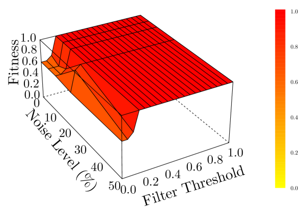
(a) Sequence Encoding

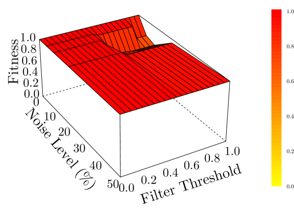
(b) IMi [26]

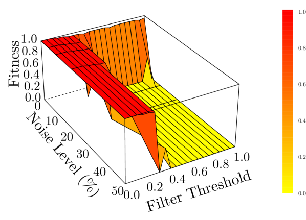
(c) ILP with Automaton Filter [20]

Figure 8: Replay-fitness measurements based on a12f0nXX.

In the charts we plot replay-fitness against the noise level and filter threshold. We additionally use a colour scheme to highlight the differences in value. Sequence Encoding Filtering has low replay-fitness values for all event logs when using a filter threshold of $0$. The replay-fitness value of the models found quickly rises to $1$ and remains $1$ for all filter threshold above $0.2$. In case of IMi, for a filter value of $1.0$ (comparable to $0.0$ for sequence encoding) we observe some values of $1$ for replay-fitness. Non-perfect replay-fitness seems to be more local, concentrated around noise levels $5\%$ and $10\%$ with corresponding threshold levels in-between $0.4$ and $0.8$. Finally, automaton-based filtering rapidly loses perfect replay-fitness when the filter threshold exceeds $0.2$. Only for a noise-level of $0$ it seems to retain high replay-values. Upon inspection it turns out the filter returns empty event logs for the corresponding threshold and noise levels.

In Figure 9 we present the precision results of the experiments with the a12f0nXX event logs.

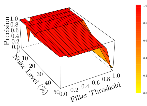
(a) Sequence Encoding

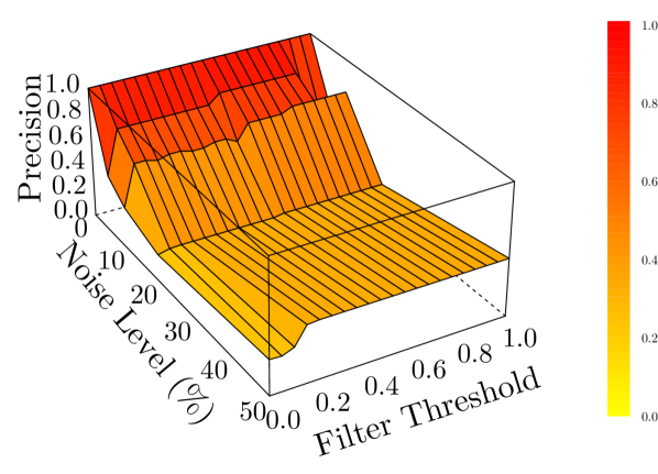
(b) IMi [26]

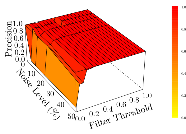
(c) ILP with Automaton Filter [20]

Figure 9: Precision measurements based on a12f0nXX.

For sequence encoding the chart shows expected behaviour, i.e. with high noise levels and high filter thresholds precision is low. There is however an unexpected drop in precision for noise-level $0$ with a filter threshold around $0.2$. The IMi filter behaves a bit more unexpected since the drop in precision seems mainly depending on the noise level rather than the filter setting. We expect the precision to be higher in case a filter threshold of $1.0$ is chosen. There is only a slight increase for the $50\%$ noise log when comparing a filter threshold of $0$ to a filter threshold of $1$. Finally, precision of the automaton filter behaves as expected, i.e., precision rapidly increases together with an increase in the filter threshold.

The replay-fitness results of the experiments with the a22f0nXX event logs are presented in Figure 10.

(a) Sequence Encoding

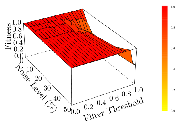
(b) IMi [26]

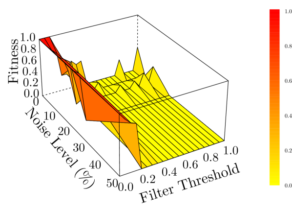
(c) ILP with Automaton Filter [20]

Figure 10: Replay-fitness measurements based on a22f0nXX.

The charts very similar behaviour to the results reported for the a12f0nXX event logs. The sequence encoding filter in 10(a) has a replay-fitness value of around $0.6$ when applying it as rigorous as possible, i.e. using $\alpha=0$. This implies that the filter even removes behaviour that is present in the ground-truth event log. For increasing filter thresholds the replay-fitness value reaches a value of $1$ rapidly, i.e., the model is able to reproduce all traces in the event log. For IMi (10(b)) we observe similar behaviour (note that the filter threshold works inverted w.r.t. sequence encoding filtering, i.e. a value of $1$ implies most rigorous filtering). However, replay-fitness drops a little earlier compared to sequence encoding filtering. Finally, automaton based filtering, depicted in 10(b), rapidly drops to $0$. Again this is due to the fact that the filter tends to return empty logs for high threshold values. Hence, the filter seems to be very sensitive around a threshold value in-between $0$ and $0.2$.

The precision results of the experiments with the a22f0nXX event logs are presented in Figure 11.

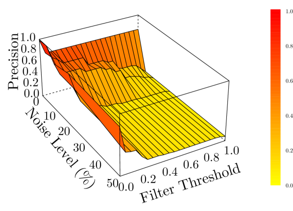
(a) Sequence Encoding

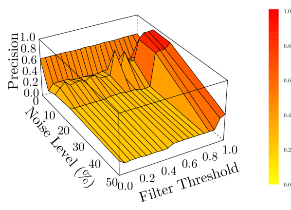
(b) IMi [26]

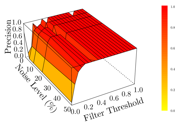
(c) ILP with Automaton Filter [20]

Figure 11: Precision measurements based on a22f0nXX.

For both the sequence encoding (11(a)) and IMi (11(b)) we observe a precision value of around $0.6$ based on the event logs without any noise. This is due to the fact that the originating model contains a loop which leads to imprecision. We observe that both sequence encoding filtering as well as IMi follow the same pattern in terms of precision. However, the drop in precision of sequence encoding filtering is more smooth than the drop in precision of IMi, i.e. there exist some spikes within the graph. Hence, the applying filtering within IMi seems to be less deterministic. Finally, the precision results for the automaton based filter are as expected. With a low threshold value we have very low precision, except when we have a $0\%$ noise level. Towards a threshold level of $0.2$ precision increases after which it maximizes out to a value of $1$. This is in line with the replay-fitness measurements.

In Figure 12 we present the replay-fitness results of the experiments with the a32f0nXX event logs. Due to excessive computation time the automaton based filter [20] is left out of the analysis.

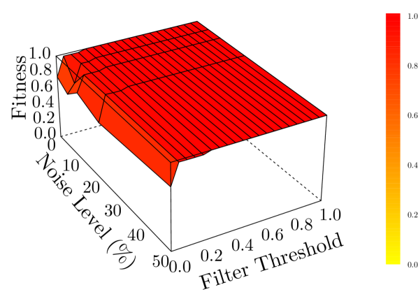
(a) Sequence Encoding

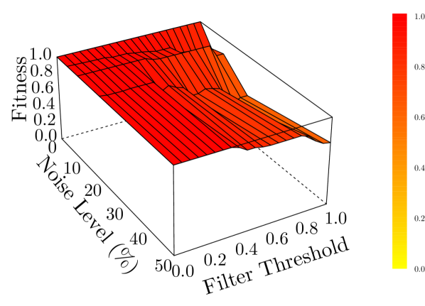
(b) IMi [26]

Figure 12: Replay-fitness measurements based on a32f0nXX.

We observe that sequence encoding filtering behaves similar to the experiments performed with the a12f0nXX and a22f0nXX event logs. The replay-fitness again quickly increase to $1$ for increasing filter threshold values. We observe that IMi seems to filter out more behaviour related to the underlying system model when the filter threshold increases.

In Figure 13 we present the precision results of the experiments with the a32f0nXX event logs.

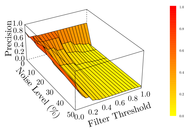
(a) Sequence Encoding

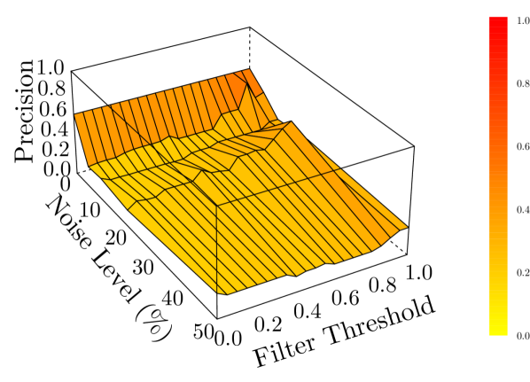
(b) IMi [26]

Figure 13: Precision measurements based on a32f0nXX.

Observe that, due to loop structures, the precision of a model that equals the originating model is only roughly $0.6$. Sequence encoding filtering shows a smooth decrease in precision when both noise and filter-thresholds are increased, which is as expected. With low noise levels and a low threshold sequence encoding seems to be able to filter out the infrequent behaviour, however, if there is too much noise and too little is removed we start finding WF-nets with self-loop places. IMi seems to result in models with a sightly higher precision compared to sequence encoding filtering. As is the case in the a22f0nXX event logs, we observe spike behaviour in precision of IMi based models hinting at non-deterministic behaviour of the filter.

Based on our experiments, we conclude that the sequence encoding filter and IMi give comparable results. However, the sequence encoding filter provides more expected results, i.e. IMi behaves somewhat deterministic. The automaton based filter does provide good results, however, sensibility of the filter threshold is much higher compared to sequence encoding filtering and IMi.

8.2 Computation time

The core of sequence encoding filtering is leaving out constraints that are likely to refer to exceptional behaviour. Thus, we reduce the size of the core ILP constraint body. Hence, we expect a decrease in computation time when applying rigorous filtering, i.e. $\kappa^{\alpha}_{max}$ with $\alpha$ towards $0$. Using RapidMiner we repeated similar experiments to the experiments performed for model quality, and measured cpu-execution time for the three techniques. However, we only use threshold values $0$, $0.25$, $0.75$ and $1$.

In Figure 14 we present the average cpu-execution time, based on 50 experiment repetitions, needed to obtain a process model from an event log.

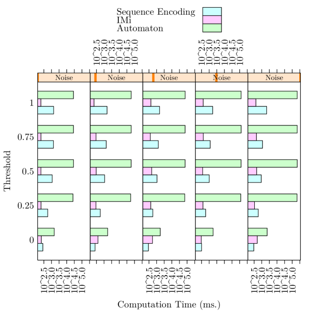
Figure 14: CPU-Execution Time (ms.) for a22f0nXX event logs (logarithmic scale).

For each level of noise we depict computation time for different filter threshold settings, $0\%$ noise is depicted in the left-most figure, $50\%$ in the right-most figure. For IMi, we measured the inductive miner algorithm with integrated filtering. For sequence encoding and automaton filtering, we measure the time needed to filter, discover a causal graph and solve underlying ILP problems. As we observe in Figure 14, IMi is fastest in all cases except for a threshold of 0 where sequence encoding tends to outperform IMi and automaton-based filtering. We observe that in all cases computation time increases when the amount of noise increases within the event logs. For sequence encoding filtering we observe that lower threshold values lead to faster computation times. This is as expected since a low threshold value removes more constraints from the ILP constraint body than a high threshold value. The automaton-based filter is slowest in all cases. The amount of noise seems to have little impact on the computation time of the automaton-based filter, it seems to be predominantly depending on the filter threshold. From Figure 14 we conclude that IMi in general out-performs sequence encoding in terms of computation time. However, sequence encoding, in turn out-performs automaton-based filtering, specifically for higher threshold settings.

8.3 Application to Real-Life Event Logs

We additionally tested the applicability of sequence encoding filtering using real-life event logs. We used two event logs, one related to the administration process of handling road fines [27] and one regarding the patient treatment of patients suspected to have sepsis [30].

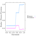
(a) Fitness and Precision

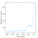
(b) Number of Arcs

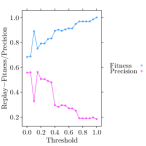
(c) Fitness and Precision

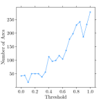
(d) Number of Arcs

Figure 15: Replay-fitness, precision and complexity based on the Road Fines log [27] (15(a) and 15(b)) and the Sepsis log [30] (15(c) and 15(d)).

The results are presented in Figure 15. In case of the Road Fines event log (figures on the left-hand side of Figure 15) we observe that replay-fitness is around $0.46$ whereas precision is around $0.4$ for $\alpha$-values from $0$ to $0.5$. The number of arcs for the models of these $\alpha$-values remains constant (as well as the number of places and the number of transitions) suggesting that the models found are the same. After this the replay-fitness increases further to around $0.8$ and reaches $1$ for an $\alpha$-level of $1$. Interestingly, precision shows a little increase around $\alpha$-levels between $0.5$ and $0.75$ after which it drops slightly below its initial value. In this case, an $\alpha$-level in-between $0.5$ and $0.75$ seems most appropriate in terms of replay-fitness, precision and simplicity.

In case of the Sepsis event log (figures on the left-hand side of Figure 15) we observe that replay-fitness and precision are roughly behaving as each-other’s inverse, i.e. replay-fitness increases whereas precision decreases for increasing $\alpha$-levels. We moreover observe that the number of arcs within the process models is steadily increasing for increasing $\alpha$-levels. In this case, an $\alpha$-level in-between $0.1$ and $0.4$ seems most appropriate in terms of replay-fitness, precision and simplicity.

Finally, for each experiment we measured the associated computation time of solving all ILP problems. In case of the Road Fines event log, solving all ILP problems takes roughly 5 seconds. In case of the Sepsis event log, obtaining a model ILP problems takes less than 1 second.

9 Conclusion

The work presented in this paper is motivated by the observation that existing region-based process discovery techniques are useful, as they are able to find non-local complex control-flow patterns. However, the techniques do not provide any structural guarantees w.r.t. the resulting process models, and, they are unable to cope with infrequent, exceptional behaviour in event logs.

The approach presented in this paper extends techniques presented in [44, 46, 45]. We have proven that our approach is able to discover relaxed sound workflow nets, i.e. we are now able to guarantee structural properties of the resulting process model. Additionally, we presented the sequence encoding filtering technique which enables us to apply filtering exceptional behaviour within the ILP-based process discovery algorithm. Our experiments confirm that the technique enables us to find Petri net structures in data consisting of exceptional behaviour, using ILP-based process discovery as an underlying technique. Sequence encoding filtering proves to be comparable to the IMi [26] approach, i.e. an integrated filter of the Inductive Miner [25], in terms of filtering behaviour. It is considerably faster than the general purpose filtering approach of [20] and less sensible to variations in the filter threshold.

Future Work

An interesting direction for future work concerns combining ILP-based process discovery techniques with other process discovery techniques. The Inductive Miner discovers sound workflow nets, however, these models are lack the ability to express complex control flow patterns such as a milestone pattern. Some of these patterns are however reconstructible using ILP-based process discovery. Hence, it is interesting to combine these approaches with possibly synergetic effects w.r.t. the process mining quality dimensions.

Another interesting approach is the development of more advanced general purpose filtering techniques. Most discovery algorithms assume the input event logs to be free of noise, infrequent and/or exceptional behaviour. Real-life event logs however typically contain a lot of such behaviour. Surprisingly, little research is performed towards filtering techniques that greatly enhance process discovery results, independent of the discovery algorithm used.

References

• [1] Aalst, W.M.P. van der: The Application of Petri Nets to Workflow Management. Journal of Circuits, Systems, and Computers 8(1), 21–66 (1998). DOI 10.1142/S0218126698000043. URL http://dx.doi.org/10.1142/S0218126698000043
• [2] Aalst, W.M.P. van der: Process Mining - Data Science in Action, Second Edition. Springer (2016). DOI 10.1007/978-3-662-49851-4. URL http://dx.doi.org/10.1007/978-3-662-49851-4
• [3] Aalst, W.M.P. van der, Adriansyah, A., Dongen, B.F. van: Replaying History on Process Models for Conformance Checking and Performance Analysis. Wiley Interdisc. Rew.: Data Mining and Knowledge Discovery 2(2), 182–192 (2012). DOI 10.1002/widm.1045. URL http://dx.doi.org/10.1002/widm.1045
• [4] Aalst, W.M.P. van der, Bolt, A., Zelst, S.J. van : RapidProM: Mine Your Processes and Not Just Your Data. CoRR abs/1703.03740 (2017). URL http://arxiv.org/abs/1703.03740
• [5] Aalst, W.M.P. van der, Hee, K.M. van, Hofstede, A.H.M. ter, Sidorova, N., Verbeek, H.M.W., Voorhoeve, M., Wynn, M.T.: Soundness of Workflow Nets: Classification, Decidability, and Analysis. Formal Asp. Comput. 23(3), 333–363 (2011). DOI 10.1007/s00165-010-0161-4. URL http://dx.doi.org/10.1007/s00165-010-0161-4
• [6] Aalst, W.M.P. van der, Hofstede, A.H.M. ter, Kiepuszewski, B., Barros, A.P.: Workflow Patterns. Distributed and Parallel Databases 14(1), 5–51 (2003). DOI 10.1023/A:1022883727209. URL http://dx.doi.org/10.1023/A:1022883727209
• [7] Aalst, W.M.P. van der, Rubin, V., Verbeek, H. M. W., Dongen, B. F. van, Kindler, E., Günther, C. W.: Process Mining: A Two-Step Approach to Balance Between Underfitting and Overfitting. Software and System Modeling 9(1), 87–111 (2010). DOI 10.1007/s10270-008-0106-z. URL http://dx.doi.org/10.1007/s10270-008-0106-z
• [8] Aalst, W.M.P. van der, Weijters, A.J.M.M., Maruster, L.: Workflow Mining: Discovering Process Models from Event Logs. IEEE Trans. Knowl. Data Eng. 16(9), 1128–1142 (2004). DOI 10.1109/TKDE.2004.47. URL http://dx.doi.org/10.1109/TKDE.2004.47
• [9] Adriansyah, A.: Aligning observed and modeled behavior. Ph.D. thesis, Eindhoven University of Technology (2014). DOI 10.6100/IR770080. URL http://dx.doi.org/10.6100/IR770080
• [10] Badouel, E., Bernardinello, L., Darondeau, P.: Polynomial Algorithms for the Synthesis of Bounded Nets. In: Mosses, P.D., Nielsen, M., Schwartzbach, M.I. (ed.) TAPSOFT’95: Theory and Practice of Software Development, 6th International Joint Conference CAAP/FASE, Aarhus, Denmark, May 22-26, 1995, Proceedings, Lecture Notes in Computer Science, vol. 915, pp. 364–378. Springer (1995). DOI 10.1007/3-540-59293-8˙207. URL http://dx.doi.org/10.1007/3-540-59293-8_207
• [11] Badouel, E., Bernardinello, L., Darondeau, P.: Petri Net Synthesis. Texts in Theoretical Computer Science. An EATCS Series. Springer (2015). DOI 10.1007/978-3-662-47967-4. URL http://dx.doi.org/10.1007/978-3-662-47967-4
• [12] Badouel, E., Darondeau, P.: Theory of Regions. In: Reisig, W., Rozenberg, G. (ed.) Lectures on Petri Nets I: Basic Models, Advances in Petri Nets, the volumes are based on the Advanced Course on Petri Nets, held in Dagstuhl, September 1996, Lecture Notes in Computer Science, vol. 1491, pp. 529–586. Springer (1996). DOI 10.1007/3-540-65306-6˙22. URL http://dx.doi.org/10.1007/3-540-65306-6_22
• [13] Bergenthum, R., Desel, J., Lorenz, R., Mauser, S.: Process Mining Based on Regions of Languages. In: Alonso, G., Dadam, P., Rosemann, M. (ed.) Business Process Management, 5th International Conference, BPM 2007, Brisbane, Australia, September 24-28, 2007, Proceedings, Lecture Notes in Computer Science, vol. 4714, pp. 375–383. Springer (2007). DOI 10.1007/978-3-540-75183-0˙27. URL http://dx.doi.org/10.1007/978-3-540-75183-0_27
• [14] Bergenthum, R., Desel, J., Lorenz, R., Mauser, S.: Synthesis of Petri Nets from Finite Partial Languages. Fundam. Inform. 88(4), 437–468 (2008). URL http://content.iospress.com/articles/fundamenta-informaticae/fi88-4-03
• [15] Bernardinello, L.: Synthesis of Net Systems. In: Marsan, M.A. (ed.) Application and Theory of Petri Nets 1993, 14th International Conference, Chicago, Illinois, USA, June 21-25, 1993, Proceedings, Lecture Notes in Computer Science, vol. 691, pp. 89–105. Springer (1993). DOI 10.1007/3-540-56863-8˙42. URL http://dx.doi.org/10.1007/3-540-56863-8_42
• [16] Bolt, A., Leoni, M. de, Aalst, W.M.P. van der: Scientific Workflows for Process Mining: Building Blocks, Scenarios, and Implementation. STTT 18(6), 607–628 (2016). DOI 10.1007/s10009-015-0399-5. URL http://dx.doi.org/10.1007/s10009-015-0399-5
• [17] Buijs, J.C.A.M., Dongen, B.F. van, Aalst, W.M.P. van der: A Genetic Algorithm for Discovering Process Trees. In: Proceedings of the IEEE Congress on Evolutionary Computation, CEC 2012, Brisbane, Australia, June 10-15, 2012, pp. 1–8. IEEE (2012). DOI 10.1109/CEC.2012.6256458. URL http://dx.doi.org/10.1109/CEC.2012.6256458
• [18] Buijs, J.C.A.M., Dongen, B.F. van, Aalst, W.M.P. van der: On the Role of Fitness, Precision, Generalization and Simplicity in Process Discovery. In: Meersman, R., Panetto, H., Dillon, T.S., Rinderle-Ma, S., Dadam, P., Zhou, X., Pearson, S., Ferscha, A., Bergamaschi, S., Crux, I.F. (ed.) On the Move to Meaningful Internet Systems: OTM 2012, Confederated International Conferences: CoopIS, DOA-SVI, and ODBASE 2012, Rome, Italy, September 10-14, 2012. Proceedings, Part I, Lecture Notes in Computer Science, vol. 7565, pp. 305–322. Springer (2012). DOI 10.1007/978-3-642-33606-5˙19. URL http://dx.doi.org/10.1007/978-3-642-33606-5_19
• [19] Carmona, J., Cortadella, J.: Process Discovery Algorithms Using Numerical Abstract Domains. IEEE Trans. Knowl. Data Eng. 26(12), 3064–3076 (2014). DOI 10.1109/TKDE.2013.156. URL http://dx.doi.org/10.1109/TKDE.2013.156
• [20] Conforti, R., Rosa, M. La, Hofstede, A.H.M. ter: Filtering Out Infrequent Behavior from Business Process Event Logs. IEEE Trans. Knowl. Data Eng. 29(2), 300–314 (2017). DOI 10.1109/TKDE.2016.2614680. URL http://dx.doi.org/10.1109/TKDE.2016.2614680
• [21] Darondeau, P.: Deriving Unbounded Petri Nets from Formal Languages. In: Sangiorgi, D., Simone, R. de (ed.) CONCUR ’98: Concurrency Theory, 9th International Conference, Nice, France, September 8-11, 1998, Proceedings, Lecture Notes in Computer Science, vol. 1466, pp. 533–548. Springer (1998). DOI 10.1007/BFb0055646. URL http://dx.doi.org/10.1007/BFb0055646
• [22] Dongen, B.F. van, Medeiros, A.K.A. de, Wen, L.: Process Mining: Overview and Outlook of Petri Net Discovery Algorithms. Trans. Petri Nets and Other Models of Concurrency 2, 225–242 (2009). DOI 10.1007/978-3-642-00899-3˙13. URL http://dx.doi.org/10.1007/978-3-642-00899-3_13
• [23] Ehrenfeucht, A., Rozenberg, G.: Partial (Set) 2-Structures. Part I: Basic Notions and the Representation Problem. Acta Inf. 27(4), 315–342 (1990). DOI 10.1007/BF00264611. URL http://dx.doi.org/10.1007/BF00264611
• [24] Ehrenfeucht, A., Rozenberg, G.: Partial (Set) 2-Structures. Part II: State Spaces of Concurrent Systems. Acta Inf. 27(4), 343–368 (1990). DOI 10.1007/BF00264612. URL http://dx.doi.org/10.1007/BF00264612
• [25] Leemans, S.J.J., Fahland, D., Aalst, W.M.P. van der: Discovering Block-Structured Process Models from Event Logs - A Constructive Approach. In: Colom, J.M., Desel, J. (ed.) Application and Theory of Petri Nets and Concurrency - 34th International Conference, PETRI NETS 2013, Milan, Italy, June 24-28, 2013. Proceedings, Lecture Notes in Computer Science, vol. 7927, pp. 311–329. Springer (2013). DOI 10.1007/978-3-642-38697-8˙17. URL http://dx.doi.org/10.1007/978-3-642-38697-8_17
• [26] Leemans, S.J.J., Fahland, D., Aalst, W.M.P. van der: Discovering Block-Structured Process Models from Event Logs Containing Infrequent Behaviour. In: Lohmann, N., Song, M., Wohed, P. (ed.) Business Process Management Workshops - BPM 2013 International Workshops, Beijing, China, August 26, 2013, Revised Papers, Lecture Notes in Business Information Processing, vol. 171, pp. 66–78. Springer (2013). DOI 10.1007/978-3-319-06257-0˙6. URL http://dx.doi.org/10.1007/978-3-319-06257-0_6
• [27] Leoni, M. de, Mannhardt, F.: Road Traffic Fine Management Process (2015). DOI 10.4121/uuid:270fd440-1057-4fb9-89a9-b699b47990f5. URL https://doi.org/10.4121/uuid:270fd440-1057-4fb9-89a9-b699b47990f5
• [28] Lorenz, R., Juhás, G.: Towards Synthesis of Petri Nets from Scenarios. In: Donatelli, S., Thiagarajan, P.S. (ed.) Petri Nets and Other Models of Concurrency - ICATPN 2006, 27th International Conference on Applications and Theory of Petri Nets and Other Models of Concurrency, Turku, Finland, June 26-30, 2006, Proceedings, Lecture Notes in Computer Science, vol. 4024, pp. 302–321. Springer (2006). DOI 10.1007/11767589˙17. URL http://dx.doi.org/10.1007/11767589_17
• [29] Lorenz, R., Mauser, S., Juhás, G.: How to Synthesize Nets from Languages - A Survey. In: Henderson, S.G., Biller, B., Hsieh, M.H., Shortle, J., Tew, J.D., Barton, R.R. (ed.) Proceedings of the Winter Simulation Conference, WSC 2007, Washington, DC, USA, December 9-12, 2007, pp. 637–647. WSC (2007). DOI 10.1109/WSC.2007.4419657. URL http://dx.doi.org/10.1109/WSC.2007.4419657
• [30] Mannhardt, F: Sepsis Cases - Event Log (2016). DOI 10.4121/uuid:915d2bfb-7e84-49ad-a286-dc35f063a460. URL https://doi.org/10.4121/uuid:915d2bfb-7e84-49ad-a286-dc35f063a460
• [31] Maruster, L., Weijters, A.J.M.M., Aalst, W.M.P. van der, Bosch, A. van den: A Rule-Based Approach for Process Discovery: Dealing with Noise and Imbalance in Process Logs. Data Min. Knowl. Discov. 13(1), 67–87 (2006). DOI 10.1007/s10618-005-0029-z. URL http://dx.doi.org/10.1007/s10618-005-0029-z
• [32] Medeiros, A.K.A. de, Dongen, B.F. van, Aalst, W.M.P. van der, Weijters, A.J.M.M.: Process Mining for Ubiquitous Mobile Systems: An Overview and a Concrete Algorithm. In: Baresi, L., Dustar, S., Gall, H.C., Matera, M. (ed.) Ubiquitous Mobile Information and Collaboration Systems, Second CAiSE Workshop, UMICS 2004, Riga, Latvia, June 7-8, 2004, Revised Selected Papers, Lecture Notes in Computer Science, vol. 3272, pp. 151–165. Springer (2004). DOI 10.1007/978-3-540-30188-2˙12. URL http://dx.doi.org/10.1007/978-3-540-30188-2_12
• [33] Munoz-Gama, J.: Conformance Checking and Diagnosis in Process Mining - Comparing Observed and Modeled Processes, Lecture Notes in Business Information Processing, vol. 270. Springer (2016). DOI 10.1007/978-3-319-49451-7. URL http://dx.doi.org/10.1007/978-3-319-49451-7
• [34] Murata, T.: Petri Nets: Properties, Analysis and Applications. Proceedings of the IEEE 77(4), 541–580 (1989). DOI 10.1109/5.24143
• [35] Reisig, W.: The Synthesis Problem. Trans. Petri Nets and Other Models of Concurrency 7, 300–313 (2013). DOI 10.1007/978-3-642-38143-0˙8. URL http://dx.doi.org/10.1007/978-3-642-38143-0_8
• [36] Schrijver, A.: Theory of Linear and Integer Programming. Wiley-Interscience series in discrete mathematics and optimization. Wiley (1999)
• [37] Solé, M., Carmona, J.: Process Mining from a Basis of State Regions. In: Lilius, J., Penczek, W. (ed.) Applications and Theory of Petri Nets, 31st International Conference, PETRI NETS 2010, Braga, Portugal, June 21-25, 2010. Proceedings, Lecture Notes in Computer Science, vol. 6128, pp. 226–245. Springer (2010). DOI 10.1007/978-3-642-13675-7˙14. URL http://dx.doi.org/10.1007/978-3-642-13675-7_14
• [38] Verbeek, H.M.W., Buijs, J.C.A.M., Dongen, B.F. van, Aalst, W.M.P. van der: XES, XESame, and ProM 6. In: Soffer, P., Proper, E. (ed.) Information Systems Evolution - CAiSE Forum 2010, Hammamet, Tunisia, June 7-9, 2010, Selected Extended Papers, Lecture Notes in Business Information Processing, vol. 72, pp. 60–75. Springer (2010). DOI 10.1007/978-3-642-17722-4˙5. URL http://dx.doi.org/10.1007/978-3-642-17722-4_5
• [39] Weerdt, J. de, Backer, M. de, Vanthienen, J., Baesens, B.: A Multi-Dimensional Quality Assessment of State-Of-The-Art Process Discovery Algorithms using Real-Life Event Logs. Inf. Syst. 37(7), 654–676 (2012). DOI 10.1016/j.is.2012.02.004. URL http://dx.doi.org/10.1016/j.is.2012.02.004
• [40] Weijters, A.J.M.M., Aalst, W.M.P. van der: Rediscovering Workflow Models from Event-Based Data using Little Thumb. Integrated Computer-Aided Engineering 10(2), 151–162 (2003). URL http://content.iospress.com/articles/integrated-computer-aided-engineering/ica00143
• [41] Weijters, A.J.M.M., Ribeiro, J.T.S.: Flexible Heuristics Miner (FHM). In: Proceedings of the IEEE Symposium on Computational Intelligence and Data Mining, CIDM 2011, part of the IEEE Symposium Series on Computational Intelligence 2011, April 11-15, 2011, Paris, France, pp. 310–317. IEEE (2011). DOI 10.1109/CIDM.2011.5949453. URL http://dx.doi.org/10.1109/CIDM.2011.5949453
• [42] Wen, L, Aalst, W.M.P. van der, Wang, J., Sun, J.: Mining Process Models with Non-Free-Choice Constructs. Data Min. Knowl. Discov. 15(2), 145–180 (2007). DOI 10.1007/s10618-007-0065-y. URL http://dx.doi.org/10.1007/s10618-007-0065-y
• [43] Wen, L., Wang. J., Aalst, W.M.P. van der, Huang, B., Sun, J.: Mining Process Models with Prime Invisible Tasks. Data Knowl. Eng. 69(10), 999–1021 (2010). DOI 10.1016/j.datak.2010.06.001. URL http://dx.doi.org/10.1016/j.datak.2010.06.001
• [44] Werf, J.M.E.M. van der, Dongen, B.F. van, Hurkens, C.A.J., Serebrenik, A.: Process Discovery using Integer Linear Programming. Fundam. Inform. 94(3-4), 387–412 (2009). DOI 10.3233/FI-2009-136. URL http://dx.doi.org/10.3233/FI-2009-136
• [45] Zelst, S.J. van, Dongen, B.F. van, Aalst, W.M.P. van der: Avoiding Over-Fitting in ILP-Based Process Discovery. In: Motahari-Nezhad, H.R., Recker, J. Weidlich, M. (ed.) Business Process Management - 13th International Conference, BPM 2015, Innsbruck, Austria, August 31 - September 3, 2015, Proceedings, Lecture Notes in Computer Science, vol. 9253, pp. 163–171. Springer (2015). DOI 10.1007/978-3-319-23063-4˙10. URL http://dx.doi.org/10.1007/978-3-319-23063-4_10
• [46] Zelst, S.J. van, Dongen, B.F. van, Aalst, W.M.P. van der: ILP-Based Process Discovery Using Hybrid Regions. In: Aalst, W.M.P. van der, Bergenthum, R., Carmona, J. (ed.) Proceedings of the ATAED 2015 Workshop, Satellite event of Petri Nets/ACSD 2015, Brussels, Belgium, June 22-23, 2015., CEUR Workshop Proceedings, vol. 1371, pp. 47–61. CEUR-WS.org (2015). URL http://ceur-ws.org/Vol-1371/paper04.pdf