Chance Constrained Optimal Power Flow with Primary Frequency Response

Abstract

Primary frequency response is provided by synchronized generators through their speed-droop governor characteristic in response to instant frequency deviations that exceed a certain threshold, also known as the governor dead zone. This paper presents an Optimal Power Flow (OPF) formulation that explicitly models i) the primary frequency response constraints using a nonlinear speed-droop governor characteristic with a dead zone and ii) chance constraints on power outputs of conventional generators and line flows imposed by the uncertainty of renewable generation resources. The proposed formulation is evaluated and compared to the standard CCOPF formulation on a modified 118-bus IEEE Reliability Test System.

I Introduction

As a result of policy initiatives and incentives, renewable generation resources have already exceeded 10% penetration levels, in terms of annual electricity produced, in some interconnections; even higher targets are expected to be reached in the forthcoming years [1]. Integrating renewable generation resources increases reserve requirements needed to deal with their uncertainty and variability and, at the same time, tends to replace conventional generation resources that are most suitable for the efficient reserve provision, [2]. Among these reserve requirements, the ability to provide sufficient primary frequency response, i.e. the automatic governor-operated response of synchronized generators intended to compensate a sudden power mismatch based on local frequency measurements, is the least studied [3]. The impacts of renewable generation resources on the secondary and tertiary reserve requirements are reviewed in [4, 5].

Data-driven studies in [6] and [7] manifestly reveal that the primary frequency response in major US interconnections has drastically reduced over the past decades and attribute this effect to increased penetrations of renewable generation resources. Primary frequency response constraints are modeled in [8] and [9]. These studies consider a nonlinear speed-droop governor characteristic with an intentional dead zone that makes it possible to preserve the primary frequency response for reacting to relatively large frequency deviations caused by sudden generation and demand failures [10]. However, the formulations in [8] and [9] ignore transmission constraints and the uncertainty of renewable generation resources that may lead to overload and capacity scarcity events when the primary frequency response is deployed.

To deal with the stochastic nature of renewable generation resources and their impacts on the secondary and tertiary reserve requirements, the standard optimal power flow (OPF) formulations have been enhanced using chance constrained programming [11], scenario-based stochastic programming [12] and robust optimization [13]. The formulation in [11] postulates that the uncertainty and variability of wind power generation resources follow a given Gaussian distribution that makes it possible to convert the Chance Constrained OPF (CCOPF) into a second-order cone program, which is then solved using a cutting-plane-based procedure. Relative to [11], the formulation in [12] is more computationally demanding since it requires computationally expensive scenario sampling, [14]. Unlike [11] and [12], the formulation in [13] disregards the likelihood of individual scenarios within a given uncertainty range and tends to yield overly conservative solutions. Based on the CCOPF formulation in [11], several extensions have been developed. Thus, [15] implements a distributionally robust CCOPF formulation that internalizes parameter uncertainty on the Gaussian distribution characterizing wind power forecast errors as explained in [16]. In [17], the CCOPF formulation is extended to accommodate corrective control actions. The formulation in [18] describes the CCOPF formulation that uses wind curtailments for self-reserve to reduce the secondary and tertiary reserve provision by conventional generation resources. In [19], the chance constraints are modified to selectively treat large and small wind power perturbations using weighting functions. Notably, the convexity of the original formulation in [11] is preserved in [17, 18, 19, 15].

The formulations in [11, 17, 18, 19, 15] have been proven to reliably and cost-efficiently deal with the uncertainty and variability imposed by renewable generation resources at a computational acceptable cost, even for realistically large networks [11, 15]. However, these formulations neglect to account for nonlinear primary frequency response policies, i.e. the dead zone of the speed-droop governor characteristic. From the reliability perspective, this may result in the inability to timely arrest a frequency decay caused by credible contingencies, [6, 20, 10]. Furthermore, ignoring nonlinear primary frequency response policies may lead to suboptimal dispatch decisions and cause unnecessary out-of-market corrections that would eventually increase the overall operating cost, [21]. This paper proposes a CCOPF formulation with a nonlinear primary frequency response policy that seeks the least-cost dispatch and primary frequency response provision among available conventional generation resources. The main contributions of this paper are:

1. The proposed CCOPF-Primary Frequency Rresponse (PFR) formulation enhances the CCOPF formulation in [11] by explicitly considering primary frequency response constraints of conventional generators.

2. As in [8] and [9], the primary frequency response is modeled using a nonlinear speed-droop governor characteristic with an intentional dead zone, i.e. the primary frequency response does not react to frequency fluctuations below a given threshold.

3. The weighted chance constraints from [19] are used to reformulate the proposed CCOPF-PFR formulation into a convex program that can be solved using off-the-shelf solvers. The CCOPF-PFR and CCOPF formulations are compared using a modification of the 118-bus IEEE Reliability Test System [22].

The rest of this paper is organized as follows. Section II describes the proposed CCOPF-PFR on the standard CCOPF from [11]. Section III describes the solution technique. Section IV compares the CCOPF-PFR and CCOPF formulations quantitatively. Section V summarizes the key findings.

II CCOPF-PFR Formulation

This section derives the CCOPF-PFR formulation. Section II-A reviews the CCOPF formulation from [11]. Next, Section II-B details a generic affine frequency control policy, which is generalized in Section II-C to include a given dead zone. Section II-D applies the weighted chance constraints from [19] to obtain the final CCOPF-PFR formulation.

II-A Standard CCOPF

As customarily done in the analysis of transmission grids, the deterministic OPF based on the DC power flow (PF) approximation is stated as follows:

$$\min_{p_{g},\phi,\theta} \sum_{i\in{\cal V}_{g}}C_{i}(p_{i})$$ (2)

s. t.

$$\sum_{i\in{\cal V}}p_{i}=0$$

$$\forall i\in{\cal V}_{g}: p_{i}\in[\underline{p}_{i},\overline{p}_{i}]$$ (3)

$$\forall i\in{\cal V}: p_{i}=\sum_{j:\{i,j\}\in{\cal E}}\phi_{ij}$$ (4)

$$\forall\{i,j\}\in{\cal E}: \phi_{ij}=\beta_{ij}(\theta_{i}-\theta_{j})$$ (6)

$$\phi_{ij}\in[-\bar{\phi}_{ij},\bar{\phi}_{ij}],$$

where the transmission grid-graph is ${\cal G}=({\cal V},{\cal E})$, where ${\cal V}$ and ${\cal E}$ denote the sets of nodes (buses) and edges (transmission lines), and ${\cal V}$ is split into three subsets: conventional generators, ${\cal V}_{g}$, loads, ${\cal V}_{l}$, and wind farms, ${\cal V}_{w}$, i.e. ${\cal V}={\cal V}_{g}\cup{\cal V}_{l}\cup{\cal V}_{w}$. Eq. (2) is optimized over the i) vector of power outputs of conventional generators, $p_{g}=(p_{i}|i\in\cal{V}_{g})$, ii) vector of transmission power flows, $\phi=(\phi_{ij}=-\phi_{ji}|\{i,j\}\in{\cal E})$, and iii) vector of voltage angles, $\theta=(\theta_{i}|i\in{\cal V})$. The input parameters include the minimum, $\underline{p}_{i}$, and the maximum, $\overline{p}_{i}$, limits on the power output of conventional generators, the vector of nodal loads, $p_{l}=(p_{i}|i\in{\cal V}_{l})$, the vector of wind power injections, $p_{w}=\rho=(\rho_{i}|i\in{\cal V}_{w})$, as well as the vector of line impedances, $(\beta_{ij},\forall\{i,j\}\in\cal{E})$ and the vector of the line power flow limits, $(\overline{\phi}_{ij},\forall\{i,j\}\in\cal{E})$. Eq. (2) minimizes the total operating cost using a convex, quadratic cost function of each conventional generator, $C_{i}(\cdot)$. The system-wide power balance is enforced by Eq. (2). Eq. (3) limits the power output of the conventional generators. The nodal power balance is enforced by Eq. (4) using the line flows computed in Eq. (6) based on the DC power flow approximation. Eq.(6) limits the line flows.

Eqs. (2)-(6) seek the least-cost solution assuming fixed power outputs of wind farms. In fact, these outputs are likely to vary due to the inherent wind speed uncertainty and variability [16] that can be accounted for as follows by using the chance constrained framework of [11, 15]:

$$\min\limits_{p_{g}^{(0)},\theta,\rho} \sum_{i\in{\cal V}_{g}}\mathbb{E}_{\rho}\left[C_{i}(p_{i})\right]$$

s. t.

$$\forall i\in{\cal V}_{g}: \mbox{Prob}_{\rho}\left[p_{i}\leq\underline{p}_{i}\right]\leq\varepsilon_{i}^{\downarrow}$$ (9)

$$\mbox{Prob}_{\rho}\left[p_{i}\geq\overline{p}_{i}\right]\leq\varepsilon_{i}^{\uparrow}$$

$$\forall\{i,j\}\in{\cal E}: \mbox{Prob}_{\rho}\left[\phi_{ij}\leq-\underline{\phi}_{ij}\right]\leq\varepsilon_{ij}^{\downarrow}$$ (11)

$$\mbox{Prob}_{\rho}\left[\phi_{ij}\geq\overline{\phi}_{ij}\right]\leq\varepsilon_{ij}^{\uparrow}.$$

where we follow [16] to describe $\rho=p_{w}$ as a random quantity represented through the exogenous statistics of the wind power. Consistently with [16] we use the term “uncertainty” in this paper to refer to wind power forecast errors (associated with the imperfection of measurement/computation/predicition tools) and the term “variability” to refer to random fluctuations of wind power output caused by natural atmospheric processes. This statistics is assumed to be Gaussian

$$\forall i\in{\cal V}_{w}: \mathbb{E}\left[\rho_{i}\right]=\bar{\rho}_{i},$$ (13)

$$\ \mathbb{E}\left[\left(\rho_{i}-\bar{\rho}_{i}\right)^{2}\right]=R_{i},$$

where $\bar{\rho}_{i}$ and $R_{i}$ are the mean and covariance. In practice, the combination of uncertainty and variability can exhibit non-Gaussian features; however, the data-driven analysis from our prior work, [16, 15], suggests that the Gaussian assumption is sufficiently accurate for CCOPF computations over a large transmission grids. One can also improve the accuracy of the Gaussian representation by introducing uncertainty sets on its parameters, see [15], or by using an out-of-sample analysis of [11] to adjust parameters $\varepsilon_{i}^{\uparrow}$, $\varepsilon_{i}^{\downarrow}$, $\varepsilon_{ij}^{\uparrow}$, and $\varepsilon_{ij}^{\downarrow}$ in a way that they would match a given Gaussian distribution to a desired non-Gaussian distribution. The optimization Eq. (II-A)-(11) assumes that $p_{l}$ remains fixed, as in Eq. (2)-(6), while $p_{g}$ depends on $\rho$. This dependency makes it possible for conventional generators to deviate from their original set points, $p_{g}^{(0)}$, to follow random wind power outputs according to a given control policy. This policy can be affine or nonlinear as discussed in Section II-B and Section II-C, respectively. Eq. (9) and (11) are chance constrained equivalents of Eq. (3) and (6), respectively. Parameters $\varepsilon_{i}^{\uparrow}$, $\varepsilon_{i}^{\downarrow}$, $\varepsilon_{ij}^{\uparrow}$, $\varepsilon_{ij}^{\downarrow}$ can be interpreted as proxies for the fraction of time (probability) when a constraint violation can be tolerated, [11]. Relative to [11, 15], the optimization Eq. (II-A)–(11) contains a number of simplifications made for the sake of clarity. First, it assumes compulsory participation of conventional generators in the frequency control provision. Second, it ignores parameter uncertainty on the probability distribution characterizing wind power generation and correlation between distribution parameters at different nodes.

II-B Affine Frequency Control

The deterministic OPF and CCOPF formulations in Section II-A are stated for a quasi-stationary (balanced) system state, characterized by $\sum_{i\in\cal{V}}p_{i}^{(0)}=0$. Random fluctuations of wind power outputs, given by $\sum_{i\in\cal{V}_{\omega}}\rho_{i}\neq 0$, forces the system imbalance, i.e. $\sum_{i\in\cal{V}}p_{i}^{(0)}\neq 0$. In other words, since this paper focuses on the optimization over time scales of minutes and longer, sub-minute transient processes (evolution from pre-disturbed state to post-disturbed state) are ignored. This simplification makes it possible to treat the frequency and power unbalances as proportional quantities, so that if there is no frequency control, the system equilibrates within a few seconds at

$$\omega=\frac{\sum_{i\in{\cal V}_{w}}\rho_{i}}{\sum_{k\in{\cal V}_{g}}\gamma_{k}},$$ (14)

where $\omega$ is a deviation from the nominal frequency and $\gamma_{k}$ is the (natural) damping coefficient of the generator $k$.

When the affine primary frequency control is activated, the conventional generators respond as

$$\forall i\in{\cal V}_{g}:\quad p_{i}^{(0)}\to p_{i}=p_{i}^{(0)}-\alpha_{i}^{(1)}\omega_{i}.$$ (15)

This response of the conventional generators force the system to equilibrate (within the same transient time scales ranging from a few seconds to tens of seconds) at

$$\omega^{(1)}=\frac{\sum_{i\in{\cal V}_{w}}\rho_{i}}{\sum_{i\in{\cal V}_{g}}(\alpha_{i}^{(1)}+\gamma_{i})},$$ (16)

where $\alpha^{(1)}_{i}$ is the primary droop coefficient (participation factor) of the conventional generator $i$. Following the primary frequency control, the secondary frequency control, also called Automatic Generation Control (AGC) [10], would be deployed within a few minutes, thus resulting in an additional affine correction to the power output of the conventional generators. Then, Eq. (15) is modified to account for the secondary frequency control deployment as follows

$$\forall i\in{\cal V}_{g}:\quad p_{i}^{(0)}\to p_{i}=p_{i}^{(0)}-\alpha_{i}^{(1)}\omega^{(1)}-\alpha_{i}^{(2)}\omega^{(2)},$$ (17)

where $\alpha^{(2)}_{i}$ is the secondary droop coefficient (participation factor) of the conventional generator $i$. Eq. (17) assumes that the additional correction is distributed among conventional generators according to $\alpha_{i}^{(2)}$ and ensures that the system is globally balanced after both the primary and secondary frequency responses are fully deployed. Note that Eq. (17) ignores the inter-area correction component to simplify notations. Combining Eq. (16) and Eq. (17) results in

$$\omega^{(2)}\sum\limits_{i\in{\cal V}_{g}}\alpha_{i}^{(2)}=\sum\limits_{i\in{\cal V}_{w}}\rho_{i}-\omega^{(1)}\sum\limits_{i\in{\cal V}_{g}}\alpha_{i}^{(1)}=\omega^{(1)}\sum\limits_{i\in{\cal V}_{g}}\gamma_{i}^{(1)},$$ (18)

It is noteworthy to note that the secondary control should be considered as a centrally-controlled addition to the locally-managed primary control, see [10].

Note that $\omega^{(1)}$ and $\omega^{(2)}$ can each be expressed in terms of $\sum_{i\in{\cal V}_{w}}\rho_{i}$ using Eq. (18). These expressions can then be combined with Eq. (17) to summarize Eq. (4)–(6)

$$\forall i\in{\cal V}:\sum\limits_{j\sim i}\beta_{ij}(\theta_{i}-\theta_{j})=\left\{\begin{array}[]{cc}p_{i}^{(0)}-\tilde{\alpha}_{i}\sum_{k\in{\cal V}_{w}}\rho_{k},&i\in{\cal V}_{g}\\ \rho_{i},&i\in{\cal V}_{w}\\ p_{i},&i\in{\cal V}_{l}\end{array}\right.$$ (19)

where $\tilde{\alpha}_{i}$ stands for the renormalized droop coefficient of the conventional generators computed according to

$$\forall i\in{\cal V}_{g}:\quad\tilde{\alpha}_{i}=\frac{\alpha_{i}^{(1)}+\alpha_{i}^{(2)}\frac{\sum\limits_{k\in{\cal G}_{g}}\gamma_{k}^{(1)}}{\sum\limits_{l\in{\cal V}_{g}}\alpha_{l}^{(2)}}}{\sum\limits_{m\in{\cal V}_{g}}(\alpha_{m}^{(1)}+\gamma_{m}^{(1)})}.$$ (20)

The renormalized droop coefficients are subject to the following integrality constraint:

$$\sum_{i\in{\cal V}_{g}}\tilde{\alpha}_{i}=1.$$ (21)

II-C Dead Zone in Chance-Constrained Primary Control

Eq. (17)–(19) assume that the primary control reacts to a frequency deviation of any size. Even though this assumption is applicable for some systems (e.g. microgrids), it does not necessarily hold for large systems, where the primary frequency control is routinely kept untarnished during normal operations and is used only for quick and relatively rare response to large disturbances, e.g. contingencies. In such systems, $\alpha_{i}^{(1)}$ depends on the size of the frequency deviation, $\omega^{(1)}$, and can be formalized as:

$$\forall i\in{\cal V}_{g}:\quad\alpha_{i}^{(1)}\rightarrow\alpha_{i}^{(1)}\left\{\begin{array}[]{cc}0,&|\omega^{(1)}|\leq\bar{\Omega}\\ 1,&\mbox{otherwise}\end{array}\right.,$$ (24)

where parameter $\overline{\Omega}$ is a frequency threshold (dead zone) for the primary frequency response. The value of this threshold can be manually chosen as it suits the needs of a particular system, [20]. Note that the dead zone makes the frequency control policy given by Eq. (24) nonlinear; hence, one generally anticipates that ignoring the nonlinearity and using the affine policy would cause some inaccuracy.

To account for the dead zone in Eq. (24), we suggest the following modification of (9)–(9):

$$\forall i\in{\cal V}_{g}: \!\mathbb{E}_{\rho}\left[\theta(\underline{p}_{i}-p_{i})\theta(\bar{\Omega}-|\omega^{(1)}|)\right]\leq\varepsilon_{i}^{(\downarrow,-)},$$ (28)

$$\!\mathbb{E}_{\rho}\left[\theta(\underline{p}_{i}-p_{i})\theta(|\omega^{(1)}|-\bar{\Omega})\right]\leq\varepsilon_{i}^{(\downarrow,+)},$$

$$\!\mathbb{E}_{\rho}\left[\theta(p_{i}-\overline{p}_{i})\theta(\bar{\Omega}-|\omega^{(1)}|)\right]\leq\varepsilon_{i}^{(\uparrow,-)},$$

$$\!\mathbb{E}_{\rho}\left[\theta(p_{i}-\overline{p}_{i})\theta(|\omega^{(1)}|-\bar{\Omega})\right]\leq\varepsilon_{i}^{(\uparrow,+)},$$

where $\theta(x)$ is the unit step function (also known as the Heaviside step function) such that $\theta(x)=1$, if $x>0$, and $\theta(x)=0$ otherwise. Eqs. (28)–(28) incorporate both the nonlinear primary frequency response and the wind power generation statistics described by $\rho$, as given in Eq. (13)-(13). Note that the parameters $\varepsilon_{i}^{(\downarrow,-)}$, $\varepsilon_{i}^{(\downarrow,+)}$, $\varepsilon_{i}^{(\uparrow,-)}$,$\varepsilon_{i}^{(\uparrow,+)}$ are defined similarly to parameters $\varepsilon_{i}^{\uparrow}$ and $\varepsilon_{i}^{\downarrow}$ in Eq. (9)-(9).

Section III shows how Eq. (28)–(28) can be represented in a computationally tractable form as one-dimensional integrals (with erf-functions in the integrands). The same transformation is applicable for Eq. (28)–(28).

II-D Weighted CCOPF

Following the method of [19] we introduce weighted chance constraints imposed at the conventional generators:

$$\forall i\in{\cal V}_{g}: \!\!\mathbb{E}_{\rho}\!\!\left[\exp\!\left(\!-\frac{p_{i}}{\underline{p}_{i}}\!\right)\theta\left(\bar{\Omega}-|\omega^{(1)}|\right)\right]\!\leq\!\varepsilon_{i}^{(\downarrow,-)},$$ (32)

$$\!\!\mathbb{E}_{\rho}\!\!\left[\exp\!\left(\!-\frac{p_{i}}{\underline{p}_{i}}\!\right)\theta\left(|\omega^{(1)}|-\bar{\Omega}\right)\right]\!\leq\!\varepsilon_{i}^{(\downarrow,+)},$$

$$\!\!\mathbb{E}_{\rho}\!\!\left[\exp\!\left(\!\frac{p_{i}}{\overline{p}_{i}}\!\right)\theta\left(\bar{\Omega}-|\omega^{(1)}|\right)\right]\!\leq\!\varepsilon_{i}^{(\uparrow,-)},$$

$$\!\!\mathbb{E}_{\rho}\!\!\left[\exp\!\left(\!\frac{p_{i}}{\overline{p}_{i}}\!\right)\theta\left(|\omega^{(1)}|-\bar{\Omega}\right)\right]\!\leq\!\varepsilon_{i}^{(\uparrow,+)}.$$

The weighted chance constraints are advantageous for the following three reasons. First, this form allows the freedom in differentiating effects of small and large violations [19]. Second, the resulting constraints are convex regardless of the input statistics (Gaussian or not) [19]. Third, it offers a computational advantage as the expectations on the left-hand side of Eqs. (32)-(32) are stated explicitly in terms of the (well tabulated) erf-functions.

Then our CCOPF-PFR formulation with the weighted chance constraints is as follows:

$$\min\limits_{p_{g}^{(0)}}\sum_{i\in{\cal V}_{g}}\mathbb{E}_{\rho}\left[C_{i}(p_{i})\right]$$ (33)

$$\forall i\in{\cal V}_{g}:$$ Eqs. (32)–(32) (34)

$$\forall\{i,j\}\in{\cal E}: \mathbb{E}_{\rho}\left[\exp\left(\!-\frac{\phi_{ij}}{\underline{\phi}_{ij}}\right)\theta\left(\bar{\Omega}\!-\!|\omega^{(1)}|\!\right)\right]\leq\!\varepsilon_{ij}^{(\downarrow,-)},$$ (36)

$$\mathbb{E}_{\rho}\left[\exp\left(\!-\frac{\phi_{ij}}{\underline{\phi}_{ij}}\right)\theta\left(|\omega^{(1)}|\!-\!\bar{\Omega}\!\right)\right]\leq\!\varepsilon_{ij}^{(\downarrow,+)},$$

$$\mathbb{E}_{\rho}\left[\exp\left(\frac{\phi_{ij}}{\overline{\phi}_{ij}}\right)\theta\left(\bar{\Omega}-|\omega^{(1)}|\right)\right]\leq\varepsilon_{ij}^{(\uparrow,-)},$$ (37)

$$\mathbb{E}_{\rho}\left[\exp\left(\frac{\phi_{ij}}{\overline{\phi}_{ij}}\right)\theta\left(|\omega^{(1)}|-\bar{\Omega}\right)\right]\leq\varepsilon_{ij}^{(\uparrow,+)}.$$ (38)

Note that parameters $\varepsilon_{ij}^{(\downarrow,-)}$, $\varepsilon_{ij}^{(\downarrow,+)}$, $\varepsilon_{ij}^{(\uparrow,-)}$,$\varepsilon_{ij}^{(\uparrow,+)}$ are defined similarly to parameters $\varepsilon_{i}^{\uparrow}$ and $\varepsilon_{i}^{\downarrow}$ in Eqs. (9)-(9).

III Solution Approach

This Section describes how the weighted chance constraints (34)-(38) can be computed efficiently. The process is illustrated on Eqs. (32)-(32) and can be extended to other chance constraints. The left-hand sides of Eq. (32)–(32) depend on $\rho_{i}$ and $\overline{\Omega}$ attaining non-zero values if $\bar{\Omega}>|\omega^{(1)}|$ and $\bar{\Omega}<|\omega^{(1)}|$, respectively. Thus, the left-hand sides can be restated as expectations over two distinct Gaussian distributions defined by the following means and covariances:

$$\mathbb{E}\left[\omega^{(1)}\right]_{\sigma}\doteq\Omega_{\sigma}=\frac{\sum_{i\in{\cal V}_{w}}\bar{\rho}_{i}}{\sum_{k\in{\cal V}_{g}}(\sigma\alpha^{(1)}_{k}+\gamma_{k})},$$ (39)

$$\mathbb{E}\left[\left(\omega^{(1)}-\Omega_{\sigma}\right)^{2}\right]_{\sigma}\doteq\Theta^{(\omega,\omega)}_{\sigma}$$

$$=\frac{\sum_{i\in{\cal V}_{w}}R_{i}}{(\sum_{k\in{\cal V}_{g}}(\sigma\alpha^{(1)}_{k}+\gamma_{k}))^{2}},$$ (40)

$$\forall i\in{\cal V}_{g}:$$

$$\mathbb{E}\left[p_{i}\right]_{\sigma}\doteq P_{\sigma;i}=p^{(0)}_{i}-\tilde{\alpha}_{i;\sigma}\sum_{j\in{\cal V}_{w}}\bar{\rho}_{j},$$ (41)

$$\mathbb{E}\left[\left(p_{i}-P_{\sigma;i}\right)\left(\omega^{(1)}-\Omega_{\sigma}\right)\right]_{\sigma}\doteq\Theta^{(p_{i},\omega)}_{\sigma}$$

$$=-\frac{\tilde{\alpha}_{i;\sigma}\sum_{j\in{\cal V}_{w}}R_{j}}{\sum_{k\in{\cal V}_{g}}(\sigma\alpha_{k}^{(1)}+\gamma_{k})}$$ (42)

$$\mathbb{E}\left[\left(p_{i}-P_{\sigma;i}\right)^{2}\right]_{\sigma}\doteq\Theta^{(p_{i},p_{i})}_{\sigma}=\left(\tilde{\alpha}_{i;\sigma}\right)^{2}\sum_{j\in{\cal V}_{w}}R_{j},$$ (43)

where $\sigma=\{0,1\}$ distinguish the case “$\omega^{(1)}$-in-range” and the case “$\omega^{(1)}$-off-range”. If $\sigma=0$, $\tilde{\alpha}_{i;\sigma}=\tilde{\alpha}_{i}$. If $\sigma=1$, $\tilde{\alpha}_{i}$ is derived from (20) using the replacement $\alpha^{(1)}=0$. It is also useful to introduce the so-called precision matrices defined as the inverse $(2\times 2)$ matrices of the covariance matrices

$$\forall i\in{\cal V}_{g}: \Phi_{\sigma;i}=\left(\begin{array}[]{cc}\Phi^{(p_{i},p_{i})}_{\sigma}&\Phi^{(p_{i},\omega)}_{\sigma}\\ \Phi^{(p_{i},\omega)}_{\sigma}&\Phi^{(\omega,\omega)}_{\sigma}\end{array}\right)\doteq(\Theta_{\sigma;i})^{-1}$$ (49)

$$=\frac{\left(\begin{array}[]{cc}\Theta^{(\omega,\omega)}_{\sigma}&-\Theta^{(p_{i},\omega)}_{\sigma}\\ -\Theta^{(p_{i},\omega)}_{\sigma}&\Theta^{(p_{i},p_{i})}_{\sigma}\end{array}\right)}{\Theta^{(p_{i},p_{i})}_{\sigma}\Theta^{(\omega,\omega)}_{\sigma}-(\Theta^{(p_{i},\omega)}_{\sigma})^{2}}.$$

Next, Eqs. (32) can be simplified as:

$$\int\limits_{-\infty}^{+\infty}dx\left(\exp\left(\frac{x}{\underline{p}_{i}-P_{0;i}}\right)-1\right)\times$$ (50)

$$\times\int\limits_{-\bar{\Omega}-\Omega_{0}}^{\bar{\Omega}-\Omega_{0}}dy\frac{\sqrt{\mbox{det}(\Phi_{0;i})}\exp\left(-\frac{1}{2}(x,y)\Phi_{0;i}\left(\begin{array}[]{c}x\\ y\end{array}\right)\right)}{2\pi}.$$ (53)

Eq. (50) is convex with respect to the set points of the conventional generators. Note that chance constraints (32)–(32), (36)–(38) can be converted to similar convex expressions.

IV Case Study

The proposed CCOPF-PFR is compared to the standard CCOPF over a modification of the 118-bus Reliability Test System [22]. The test system includes 54 conventional generation resources and 186 transmission lines. Additionally, this system includes 9 wind farms with the forecasted total power output of 1,053 MW as itemized in Table I. The mean and standard deviation of the wind power outputs are set to 0% and 10% of the power forecast at each wind farm. The power flow limit of each transmission line is reduced by 25% of its rated value and the active power demand is increased by 10% at each bus. The droop coefficients (participation factors) of each conventional generator for each regulation interval are set to $1/N_{g}$, where $N_{g}$ is the number of conventional generators, i.e. $\alpha_{i}^{(1)}=\alpha_{i}^{(2)}=1/N_{g},\forall i\in\mathcal{V}_{g}$. The value of the dead zone for the primary frequency response is 100 MW and the likelihood of the constraint violations is set to $\varepsilon_{i}^{\downarrow}=\varepsilon_{i}^{\uparrow}=\varepsilon,\forall i\in{\cal V}_{g},$ and $\varepsilon_{ij}^{\uparrow}=\varepsilon_{ij}^{\downarrow}=\varepsilon,\forall\left\{i,j\right\}\in{\cal E}$. Both the CCOPF and CCOPF-PFR formulations are implemented in Julia [23] using the JumpChance package resolved using a 1.6 Ghz Intel Core i5 processor with 8GB of RAM.

TABLE I: Wind Power Forecast at Wind Farms ($\overline{\omega}$, MW)

bus #	3	8	11	20	24	38	43	49	50
$\overline{\omega}$	70	147	102	105	113	250	118	76	72

IV-A Comparison of the CCOPF and CCOPF-PFR solution

TABLE II: Objective Function Values and CPU Times for the CCOPF and CCOPF-PFR Formulations

$\varepsilon$	Objective function, $		CPU time, s
	CCOPF	CCOPF-PFR	CCOPF	CCOPF-PFR
$10^{-1}$	91,504.8	94,757.3 (+3.55%)∗	10.4	17.3
$10^{-2}$	92,984.6	94,861.5 (+2.02%)∗	11.9	18.1
$10^{-3}$	94658.7	96,045.3 (+1.46%)∗	12.1	19.4
$10^{-4}$	97,615.1	98,101.4 (+0.49%)∗	21.7	18.9
∗ – the percentage values are relative to the CCOPF formulation.

First, the CCOPF and CCOPF-PFR formulations are solved for different values of $\varepsilon$. Table II compares the objective functions of these formulations and their CPU times. In general, the CCOPF-PFR consistently yields a more expensive solution since it has a more constrained feasible region due to the active PFR constraints. As the value of parameter $\varepsilon$ reduces so does the relative difference between the objective function of the CCOPF and CCOPF-PFR formulations. This observation suggests that a nonlinear primary frequency response policy comes at a lower cost for risk-averse OPF solutions. At the same time, the computing times reported in Table II suggest that a higher level of modeling accuracy in the CCOPF-PFR formulation comes at a minimal increase in the computation time.

Second, the CCOPF and CCOPF-PFR solutions presented in Table II are tested over a set of 10,000 random realizations of wind power forecast errors, where each random realization is sampled using the multivariate Gaussian distribution. In each test, the decisions produced by the CCOPF and CCOPF-PFR are fixed and the constraint violations are calculated.

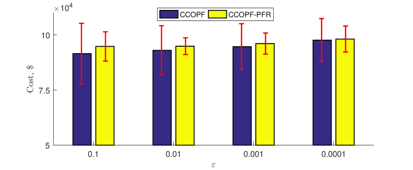
Figure 1: Comparison of the CCOPF and CCOPF-PFR formulations in terms of the expected costs (vertical bars) and standard deviations (error bars) for different values of parameter $\varepsilon$.

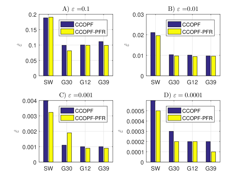
Figure 2: Empirical violations of chance constraints on conventional generators, $\hat{\varepsilon}$, for different values of parameter $\varepsilon$. Label SW (system-wide) denotes the fraction of realizations that lead to a violation of at least one chance constraint in the entire transmission system. Labels G30, G12 and G38 denote the fraction of realizations that lead to violations of chance constraints for the maximum power output at conventional generators G30 ($\overline{p}_{i}$ = 805.2 MW), G12 ($\overline{p}_{i}$ = 413.9 MW) and G38 ($\overline{p}_{i}$ =104.0 MW)

Fig. 1 displays the excepted operating cost and its standard deviation observed over 10,000 tests for the CCOPF and CCOPF-PFR formulations. For both formulations the expected operating cost and its standard deviation monotonically change with the value of parameter $\varepsilon$. Thus, the expected operating cost under both formulations gradually increases for higher values of parameter $\varepsilon$, while the standard deviation reduces. Notably, in all instances displayed in Fig. 1 the expected cost of the CCOPF-PFR formulation is greater than the expected cost of the CCOPF formulation. As in the cost results presented in Table II, the gap between the expected costs of both formulations reduces for higher values of parameter $\varepsilon$. On the other hand, the CCOPF-PFR formulation leads to a lower standard deviation in all instances, which suggests that the CCOPF-PFR formulation is more robust and cost-efficient for accommodating relatively large wind power forecast errors. A more expensive and conservative CCOPF-PFR solution leads to less violations of chance constraints on conventional generators as shown in Fig. 2. The number of violations reduces for the entire system and for individual generators of different sizes. Therefore, the CCOPF-PFR formulation is more effective in accommodating deviations from the forecasted values. Furthermore, there is no noticeable difference in violations of the chance constraints over line flows between the CCOPF and CCOPF-PFR formulation. This observation suggests that the main effect of CCOPF-PFR is in improving compliance on the supply side with the operating limits.

V Conclusion

In this paper, the CCOPF formulation from [11] has been enhanced to explicitly model constraints associated with the primary frequency response based on a nonlinear speed-droop governor characteristic of conventional generators. The proposed CCOPF-PFR formulation has been compared to the original CCOPF formulation on a modification of the 118-bus IEEE Reliability Test System [22]. This comparison indicates that modeling a nonlinear speed-droop governor characteristic leads to only a rather modest increase of the expected operating cost, while improving adaptability of the dispatch solutions to relative large deviations from the forecast. The increased adaptability of the CCOPF-PFR formulation is observed in reduction of the chance constraints violations on the conventional generators and it is also seen in lower standard deviations of the operating cost. We have also observed that the proposed CCOPF-PFR and standard CCOPF formulations are comparable in terms of required computational resources.

This work can be extended in several ways:

• The PFR constraints assume that generators instantly react to a power imbalance, i.e. there is no time delay, which can be observed in practice [10]. Modeling this delay is a possible extension of the proposed work aimed at improving the accuracy.

• PFR constraints can be generalized to explicitly account for instant power flow fluctuations over transmission lines adjusted to the generator. This can be without additional communication constraints by using local measurements.

• The proposed CCOPF-PFR model can be enhanced to include an endogenous contingency reserve assessment, e.g. a probabilistic security-constrained framework [24]. The proposed primary frequency response constraints can be used to accurately estimate the minimum response requirement and its allocation instead of using the deterministic heuristics [20].

• The proposed CCOPF-PFR model relies on lossless DC power flows, which needs to and seemingly can be extended to account for power losses, reactive power flows, and voltage fluctuations via linear or quadratic AC power flow approximations.

References

- [1] F. Pazheri, M. Othman, and N. Malik, “A review on global renewable electricity scenario,” Renewable and Sustainable Energy Reviews, vol. 31, pp. 835 – 845, 2014.
- [2] N. Troy, E. Denny, and M. O’Malley, “Base-load cycling on a system with significant wind penetration,” IEEE Tran. Pwr. Syst., vol. 25, no. 2, pp. 1088–1097, May 2010.
- [3] J. Eto. Use of a frequency response metric to assess the planning and operating requirements for reliable integration of variable renewable generation. [Online]. Available: https://www.ferc.gov/industries/electric/indus-act/reliability/frequencyresponsemetrics-report.pdf
- [4] Y. V. Makarov, C. Loutan, J. Ma, and P. de Mello, “Operational impacts of wind generation on california power systems,” IEEE Tran. Pwr. Syst., vol. 24, no. 2, pp. 1039–1050, May 2009.
- [5] Y. Dvorkin, D. S. Kirschen, and M. A. Ortega-Vazquez, “Assessing flexibility requirements in power systems,” IET Generation, Transmission Distribution, vol. 8, no. 11, pp. 1820–1830, 2014.
- [6] P. Du and Y. Makarov, “Using disturbance data to monitor primary frequency response for power system interconnections,” IEEE Tran. Pwr. Syst., vol. 29, no. 3, pp. 1431–1432, May 2014.
- [7] J. W. Ingleson and E. Allen, “Tracking the eastern interconnection frequency governing characteristic,” in IEEE PES General Meeting, July 2010, pp. 1–6.
- [8] R. Doherty, G. Lalor, and M. O’Malley, “Frequency control in competitive electricity market dispatch,” IEEE Tran. Pwr. Syst., vol. 20, no. 3, pp. 1588–1596, Aug 2005.
- [9] J. F. Restrepo and F. D. Galiana, “Unit commitment with primary frequency regulation constraints,” IEEE Tran. Pwr. Syst., vol. 20, no. 4, pp. 1836–1842, Nov 2005.
- [10] N. Jaleeli, L. S. VanSlyck, D. N. Ewart, L. H. Fink, and A. G. Hoffmann, “Understanding automatic generation control,” pp. 1106–1122, 1992.
- [11] D. Bienstock, M. Chertkov, and S. Harnett, “Chance-constrained optimal power flow: Risk-aware network control under uncertainty,” SIAM Review, vol. 56, no. 3, pp. 461–495, 2014.
- [12] Y. Yuan, Q. Li, and W. Wang, “Optimal operation strategy of energy storage unit in wind power integration based on stochastic programming,” IET Ren. Pwr. Gen., vol. 5, no. 2, pp. 194–201, March 2011.
- [13] R. A. Jabr, “Adjustable robust opf with renewable energy sources,” IEEE Tran. Pwr. Syst., vol. 28, no. 4, pp. 4742–4751, Nov 2013.
- [14] Y. Dvorkin, Y. Wang, H. Pandzic, and D. Kirschen, “Comparison of scenario reduction techniques for the stochastic unit commitment,” in 2014 IEEE PES Gen. Meet., July 2014, pp. 1–5.
- [15] M. Lubin, Y. Dvorkin, and S. Backhaus, “A robust approach to chance constrained optimal power flow with renewable generation,” IEEE Tran. Pwr. Syst., vol. 31, no. 5, pp. 3840–3849, Sept 2016.
- [16] Y. Dvorkin, M. Lubin, S. Backhaus, and M. Chertkov, “Uncertainty sets for wind power generation,” IEEE Tran. Pwr. Syst., vol. 31, no. 4, pp. 3326–3327, July 2016.
- [17] L. Roald, S. Misra, T. Krause, and G. Andersson, “Corrective control to handle forecast uncertainty: A chance constrained optimal power flow,” IEEE Tran. Pwr. Syst., vol. 32, no. 2, pp. 26–37, March 2017.
- [18] L. Roald, G. Andersson, S. Misra, M. Chertkov, and S. Backhaus, “Optimal power flow with wind power control and limited expected risk of overloads,” in 2016 Power Systems Computation Conference (PSCC), June 2016, pp. 1–7.
- [19] L. Roald, S. Misra, M. Chertkov, and G. Andersson, “Optimal power flow with weighted chance constraints and general policies for generation control,” in 2015 54th IEEE Conference on Decision and Control (CDC), Dec 2015, pp. 6927–6933.
- [20] Y. Dvorkin, P. Henneaux, D. S. Kirschen, and H. Pandzic, “Optimizing primary response in preventive security-constrained optimal power flow,” IEEE Systems Journal, vol. PP, no. 99, pp. 1–10, 2016.
- [21] Y. M. Al-Abdullah, M. Abdi-Khorsand, and K. W. Hedman, “The role of out-of-market corrections in day-ahead scheduling,” IEEE Tran. Pwr. Syst., vol. 30, no. 4, pp. 1937–1946, July 2015.
- [22] R. D. Christie. Power systems test case archive. [Online]. Available: http://www2.ee.washington.edu/research/pstca/pf118/pg_tca118bus.htm
- [23] M. Lubin and I. Dunning, “Computing in operations research using julia,” INFORMS J. on Comp., vol. 27, no. 2, pp. 238–248, 2015.
- [24] R. Fernandez-Blanco, Y. Dvorkin, and M. A. Ortega-Vazquez, “Probabilistic security-constrained unit commitment with generation and transmission contingencies,” IEEE Tran. Pwr. Syst., vol. 32, no. 1, pp. 228–239, Jan 2017.