Up, down, and strange nucleon axial form factors from lattice QCD

Abstract

We report a calculation of the nucleon axial form factors $G_{A}^{q}(Q^{2})$ and $G_{P}^{q}(Q^{2})$ for all three light quark flavors $q\in\{u,d,s\}$ in the range $0\leq Q^{2}\lesssim 1.2\text{ GeV}^{2}$ using lattice QCD. This work was done using a single ensemble with pion mass 317 MeV and made use of the hierarchical probing technique to efficiently evaluate the required disconnected loops. We perform nonperturbative renormalization of the axial current, including a nonperturbative treatment of the mixing between light and strange currents due to the singlet-nonsinglet difference caused by the axial anomaly. The form factor shapes are fit using the model-independent $z$ expansion. From $G_{A}^{q}(Q^{2})$, we determine the quark contributions to the nucleon spin and axial radii. By extrapolating the isovector $G_{P}^{u-d}(Q^{2})$, we obtain the induced pseudoscalar coupling relevant for ordinary muon capture and the pion-nucleon coupling constant. We find that the disconnected contributions to $G_{P}$ form factors are large, and give an interpretation based on the dominant influence of the pseudoscalar poles in these form factors.

I Introduction

The axial and induced pseudoscalar form factors, $G_{A}^{q}(Q^{2})$ and $G_{P}^{q}(Q^{2})$, parameterize matrix elements of the axial current between proton states:

$$\langle p^{\prime},\lambda^{\prime}|A_{\mu}^{q}|p,\lambda\rangle=\bar{u}(p^{\prime},\lambda^{\prime})\left[\gamma_{\mu}G_{A}^{q}(Q^{2})+\frac{(p^{\prime}-p)_{\mu}}{2m_{N}}G_{P}^{q}(Q^{2})\right]\gamma_{5}u(p,\lambda),$$ (1)

where $Q^{2}=-(p^{\prime}-p)^{2}$ and $A_{\mu}^{q}=\bar{q}\gamma_{\mu}\gamma_{5}q$. It has been shown that $G_{A}^{q}(Q^{2})$ can be interpreted as the two-dimensional Fourier transform of the difference $q_{\uparrow}(\mathbf{b}_{\perp})+\bar{q}_{\uparrow}(\mathbf{b}_{\perp})-q_{\downarrow}(\mathbf{b}_{\perp})-\bar{q}_{\downarrow}(\mathbf{b}_{\perp})$ between transverse densities of helicity aligned and anti-aligned quarks plus antiquarks in a longitudinally polarized nucleon, in the infinite momentum frame Burkardt:2002hr .

At $Q^{2}=0$, the axial form factor gives the fractional contribution from the spin of quarks $q$ and $\bar{q}$ to the proton’s spin, which can also be obtained from a moment of polarized parton distribution functions:

$$\Delta q\equiv g_{A}^{q}\equiv G_{A}^{q}(0)=\int_{0}^{1}dx\left(\Delta q(x)+\Delta\bar{q}(x)\right).$$ (2)

Understanding the constituents of the proton’s spin has been of great interest ever since the European Muon Collaboration found, by measuring the spin asymmetry in polarized deep inelastic scattering, that the total contribution from quark spin to the proton’s spin is less than half Ashman:1987hv .

Axial form factors naturally arise in the interactions of nucleons with $W$ and $Z$ bosons. Assuming isospin symmetry, the $W$ boson is sensitive to the $u-d$ flavor combination, whereas the $Z$ boson is also sensitive to strange quarks. Neutron beta decay, mediated by $W$-boson exchange, is used to determine the “axial charge” $g_{A}\equiv g_{A}^{u-d}$. Quasielastic neutrino scattering, $\nu n\to\ell^{-}p$ or $\bar{\nu}p\to\ell^{+}n$, has been used to measure the isovector axial form factor $G_{A}^{u-d}(Q^{2})$, whereas elastic neutrino scattering is also sensitive to $G_{A}^{s}(Q^{2})$. The shape of the isovector axial form factor is often assumed to be a dipole, $G_{A}^{u-d}(Q^{2})=g_{A}/(1+Q^{2}/m_{A}^{2})^{2}$; rather than assume a dipole, we will use a more general fit and characterize the shape using the squared axial radii $(r_{A}^{2})^{q}$. These are defined from the slope of the form factors at zero momentum transfer:

$$G_{A}^{q}(Q^{2})=g_{A}^{q}\left(1-\frac{1}{6}(r_{A}^{2})^{q}Q^{2}+O(Q^{4})\right).$$ (3)

The ordinary “axial radius” is the isovector one, $r_{A}\equiv\sqrt{(r_{A}^{2})^{u-d}}$; in the dipole model, $r_{A}^{2}=12/m_{A}^{2}$. It can also be determined from pion electroproduction, using chiral perturbation theory Bernard:2001rs .

In addition to the valence up and down quarks, quantum fluctuations cause other quarks to play a role in the structure of nucleons; the strange quark is the next lightest, and is expected to be the next most important. In this paper, we report a calculation of the nucleon axial form factors using a single lattice QCD ensemble. This calculation includes both quark-connected and disconnected diagrams, which allows us to determine the up, down, and strange form factors. Using the same dataset, we previously reported a high-precision calculation of the strange nucleon electromagnetic form factors Green:2015wqa .

A lattice QCD study of the axial form factors of the nucleon is timely not least in view of experimental efforts underway using the MicroBooNE liquid Argon time-projection chamber, which, in particular, will be able to map out the strange axial form factor of the nucleon to momentum transfers as low as $Q^{2}=0.08\text{ GeV}^{2}$ Papavassiliou:2009zz . This is achieved by combining neutrino-proton neutral and charged current scattering cross section measurements with available polarized electron-proton/deuterium cross section data, and is expected to reduce the experimental uncertainty of the extrapolated value at $Q^{2}=0$, i.e., the strange quark spin contribution $\Delta s$, by an order of magnitude. Such an extraction is complementary to polarized DIS determinations that access the strange quark helicity distribution function, but suffer from lack of coverage at low and high momentum fraction $x$ when evaluating the first $x$-moment. The $Q^{2}$ range explored by the MicroBooNE experiment, between $Q^{2}=0.08\text{ GeV}^{2}$ and about $Q^{2}=1\text{ GeV}^{2}$, matches the range covered by the present lattice calculation well, enabling a future comparison of the $Q^{2}$-dependence obtained for the strange axial form factor.

This paper is organized as follows. Section II describes our methodology: the approach used to isolate the nucleon ground state and determine the form factors, the methods used to determine the numerically-challenging disconnected diagrams, the details of the lattice ensemble, and the fits to the $Q^{2}$-dependence of the form factors using the $z$ expansion. The unwanted contributions from excited states to the different observables are examined in detail, and the estimation of systematic uncertainty is described. Our nonperturbative calculation of the renormalization factors, including a nonperturbative treatment of the flavor singlet case, is presented in Sec. III. The main results are in Sec. IV: the axial and induced pseudoscalar form factors for light and strange quarks, as well as the quark contributions to the nucleon spin. Finally, we present our conclusions in Sec. V. In an appendix, we give the parameters for our fits to the form factors.

II Lattice methodology

II.1 Computation of matrix elements

To determine nucleon matrix elements, we compute two-point and three-point functions,

$$C_{\text{2pt}}(\vec{p},t)=\sum_{\vec{x}}e^{-i\vec{p}\cdot\vec{x}}\operatorname{Tr}\left[\Gamma_{\text{pol}}\langle\chi(\vec{x},t)\bar{\chi}(\vec{0},0)\rangle\right]$$ (4)

$$C_{\text{3pt}}^{A_{\mu}^{q}}(\vec{p},\vec{p}\,^{\prime},\tau,T)=\sum_{\vec{x},\vec{y}}e^{-i\vec{p}\,^{\prime}\cdot\vec{x}}e^{i(\vec{p}\,^{\prime}-\vec{p})\cdot y}\operatorname{Tr}\left[\Gamma_{\text{pol}}\langle\chi(\vec{x},T)A_{\mu}^{q}(\vec{y},\tau)\bar{\chi}(\vec{0},0)\rangle\right],$$ (5)

where $\chi=\epsilon^{abc}(\tilde{u}^{T}_{a}C\gamma_{5}\frac{1+\gamma_{4}}{2}\tilde{d}_{b})\tilde{u}_{c}$ is a proton interpolating operator and $\Gamma_{\text{pol}}$ is a spin and parity projection matrix. In the interpolating operator, we use Wuppertal-smeared Gusken:1989qx quark fields $\tilde{q}=(\frac{1+\alpha H}{1+6\alpha})^{N}q$, where $H$ is the nearest-neighbor gauge-covariant hopping matrix constructed using spatially APE-smeared Albanese:1987ds gauge links.

The proton ground state can be obtained in the limit where all time separations $t$, $\tau$, and $T-\tau$ are large. In this limit, the following ratio does not depend on the time separations or on the interpolating operator:

$$R_{\mu}^{q}(\vec{p},\vec{p}\,^{\prime},\tau,T) \equiv\frac{C_{\text{3pt}}^{A_{\mu}^{q}}(\vec{p},\vec{p}\,^{\prime},\tau,T)}{\sqrt{C_{\text{2pt}}(\vec{p},T)C_{\text{2pt}}(\vec{p}\,^{\prime},T)}}\sqrt{\frac{C_{\text{2pt}}(\vec{p},T-\tau)C_{\text{2pt}}(\vec{p}\,^{\prime},\tau)}{C_{\text{2pt}}(\vec{p}\,^{\prime},T-\tau)C_{\text{2pt}}(\vec{p},\tau)}}$$ (6)

$$=M_{\mu}^{q}(\vec{p},\vec{p}\,^{\prime})+O(e^{-\Delta E_{10}(\vec{p})\tau})+O(e^{-\Delta E_{10}(\vec{p}\,^{\prime})(T-\tau)}),$$

where $M_{\mu}^{q}(\vec{p},\vec{p}\,^{\prime})$ contains the desired nucleon matrix element $\langle\vec{p}\,^{\prime},\lambda^{\prime}|A_{\mu}^{q}|\vec{p},\lambda\rangle$ (with spins depending on $\Gamma_{\text{pol}}$) and some kinematic factors (see, e.g., Green:2014xba ), and $\Delta E(\vec{p})$ is the energy gap between the ground and lowest excited state with momentum $\vec{p}$.

For each source-sink separation $T$, for the ratio-plateau method, we take the average of the central two or three points $R_{\mu}^{q}(\vec{p},\vec{p}\,^{\prime},\tau,T)$ near $\tau=T/2$. This gives an estimate of $M_{\mu}^{q}(\vec{p},\vec{p}\,^{\prime})$ (and thus the nucleon matrix element) with a systematic error coming from excited-state contamination that decays exponentially as $e^{-\Delta E_{\text{min}}T/2}$, where $\Delta E_{\text{min}}=\min\{\Delta E_{10}(\vec{p}),\Delta E_{10}(\vec{p}\,^{\prime})\}$. We also use the summation method, computing the sums

$$S^{q}_{\mu}(\vec{p},\vec{p}\,^{\prime},T)\equiv a\sum_{\tau/a=1}^{T/a-1}R^{q}_{\mu}(\vec{p},\vec{p}\,^{\prime},\tau,T)=c+TM_{\mu}^{q}(\vec{p},\vec{p}\,^{\prime})+O(Te^{-\Delta E_{\text{min}}T}).$$ (7)

Fitting the slope with respect to $T$ yields an estimate of $M_{\mu}^{q}(\vec{p},\vec{p}\,^{\prime})$ that has a greater suppression of unwanted excited-state contributions Capitani:2010sg ; Bulava:2010ej , which now decay as $Te^{-\Delta E_{\text{min}}T}$.

For each $Q^{2}$, we construct a system of equations parameterizing the corresponding set of matrix elements of the axial current with $G_{A}(Q^{2})$ and $G_{P}(Q^{2})$. We combine equivalent matrix elements to improve the condition number Syritsyn:2009mx , and then solve the resulting overdetermined system of equations Hagler:2003jd . This approach makes use of all available data to minimize the statistical uncertainty. In particular, for disconnected diagrams, we are able to compute correlators for all polarizations and all equivalent momenta, maximizing the amount of averaging.

II.2 Disconnected diagrams

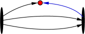
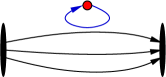
Figure 1: Two classes of quark contractions for $C_{\text{3pt}}$. Left: connected, which is evaluated using a sequential propagator through the sink (shown in blue). Right: disconnected, where the loop containing the axial current is evaluated stochastically.

There are two kinds of quark contractions that contribute to $C_{\text{3pt}}$: connected and disconnected, shown in Fig. 1. We evaluate the former exactly for each source on each gauge configuration, using sequential propagators through the sink Martinelli:1988rr . For the latter, we perform a stochastic evaluation of the disconnected loop,

$$T^{q}_{\mu}(\vec{k},t)\equiv-\sum_{\vec{x}}e^{i\vec{k}\cdot\vec{x}}\operatorname{Tr}\left[\gamma_{\mu}\gamma_{5}D^{-1}_{q}(x,x)\right],$$ (8)

where $D_{q}$ is the lattice Dirac operator with a fixed gauge background and $x=(\vec{x},t)$. We then obtain the disconnected contribution to $C_{\text{3pt}}$ from the correlation between this loop and the nucleon two-point function.

To evaluate the disconnected loop, we generate noise fields $\eta_{a\alpha}(x)$ that have color, spin, and space-time indices but with support only on a single timeslice, $t$. We use one $\mathbb{Z}_{2}+i\mathbb{Z}_{2}$ noise vector for each chosen timeslice and gauge configuration, i.e., the components of $\eta$ are randomly chosen from $\{\frac{1+i}{\sqrt{2}},\frac{1-i}{\sqrt{2}},\frac{-1+i}{\sqrt{2}},\frac{-1-i}{\sqrt{2}}\}$. As a result, the diagonal elements of $\eta\eta^{\dagger}$ are equal to 1, and the off-diagonal elements are random with expectation value zero. To reduce noise by replacing statistical zeros with exact zeros in targeted off-diagonal components of $\eta\eta^{\dagger}$, we use color and spin dilution Wilcox:1999ab ; Foley:2005ac , as well as hierarchical probing Stathopoulos:2013aci . The former makes use of a complete set of twelve projectors in color and spin space, $P_{d}$, such that $P_{d}\eta$ has support on only one color and one spin component. The latter makes use of $N_{\text{hvec}}$ specially-constructed spatial Hadamard vectors, $z_{n}$, that provide a scheme for progressively eliminating the spatially near-diagonal contributions to the noise. Combining these yields $12N_{\text{hvec}}$ modified noise fields,

$$\eta^{[d,n]}_{a\alpha}(\vec{x})=\sum_{b,\beta}(P_{d})^{b\beta}_{a\alpha}z_{n}(\vec{x})\eta_{b\beta}(\vec{x}).$$ (9)

We use these as sources for quark propagators, $\psi^{[d,n]}_{q}=D^{-1}_{q}\eta^{[d,n]}$, and obtain an estimator for $T_{\mu}^{q}(\vec{k},t)$:

$$\frac{-1}{N_{\text{hvec}}}\sum_{d,n}\sum_{\vec{x}}e^{i\vec{k}\cdot\vec{x}}\eta^{[d,n]\dagger}(\vec{x},t)\gamma_{\mu}\gamma_{5}\psi^{[d,n]}_{q}(\vec{x},t).$$ (10)

We will separately consider the connected and disconnected contributions to nucleon matrix elements of the light quark axial current. Although the individual contributions are unphysical, they can be understood using partially quenched QCD Bernard:1993sv , by introducing a third degenerate light quark $r$ and a corresponding ghost quark to cancel its fermion determinant in the path integral. The disconnected contribution to a nucleon three-point function with current $A_{\mu}^{u}$ or $A_{\mu}^{d}$ is equal to a nucleon three-point function with $A_{\mu}^{r}$. Since it was shown in Ref. Bernard:2013kwa that partially quenched staggered fermions have a bounded transfer matrix, we expect that for our case as well we can separately isolate the ground state in the connected and disconnected contributions to three-point functions, i.e., that Eq. (6) applies to $A_{\mu}^{r}$. In Section III we will also discuss renormalization of $A_{\mu}^{r}$.

II.3 Lattice ensemble and calculation setup

We use a single lattice ensemble with a tree-level Symanzik improved gauge action ($\beta=6.1$) and 2+1 flavors of clover-improved Wilson fermions that couple to the gauge links after stout smearing (one step with $\rho=0.125$). The improvement parameters are set to their tadpole-improved tree-level values. The lattice size is $32^{3}\times 96$ and the bare quark masses are $am_{s}=-0.245$ and $am_{ud}=-0.285$.

Based on the $\Upsilon(2S)-\Upsilon(1S)$ energy splitting computed using lattice NRQCD, the lattice spacing is $a=0.11403(77)$ fm. The strange quark mass is close to its physical value: the mass of the unphysical $\eta_{s}$ meson is 672(3)(5) MeV, which is within 5% of its value determined for physical quark masses Dowdall:2011wh . The light quark mass is heavier than physical, producing a pion mass of 317(2)(2) MeV. The volume is quite large, such that $m_{\pi}L_{s}\approx 5.9$, and we thus expect finite-volume effects to be highly suppressed.

We performed calculations using 1028 gauge configurations, on each of which we chose six equally-spaced source timeslices. For each source timeslice $t_{0}$, we used two positions $(\vec{x}_{1},t_{0})$ and $(\vec{x}_{2},t_{0})$ as sources for three-point functions. We placed nucleon sinks in both the forward and backward directions on timeslices $t_{0}\pm T$ to double statistics and obtain a total of 24672 samples, and used five source-sink separations $T/a\in\{6,8,10,12,14\}$. We computed disconnected loops on timeslices $t_{0}+\tau$ displaced only in the forward direction from each source timeslice, yielding 6168 timeslice samples; the source-operator separations $\tau$ and number of Hadamard vectors for each flavor are listed in Tab. 1. For each source timeslice, we computed sixteen two-point functions from source positions $(\vec{x}_{i},t_{0})$, $i=1,\dots,16$, yielding 98688 samples for correlating with the disconnected loops. We imposed two constraints on our choice of momenta: $(\vec{p}\,^{\prime}-\vec{p})^{2}\leq 10(\frac{2\pi}{L_{s}})^{2}$ and $(\vec{p})^{2},(\vec{p}\,^{\prime})^{2}\leq 6(\frac{2\pi}{L_{s}})^{2}$. For the connected diagrams we used two sink momenta, $\vec{p}\,^{\prime}=\vec{0}$ and $\vec{p}\,^{\prime}=\frac{2\pi}{L_{s}}(-1,0,0)$, and all source momenta compatible with the constraints. For the disconnected diagrams we used all combinations of $\vec{p}$ and $\vec{p}\,^{\prime}$ compatible with the constraints, with the restriction that each $Q^{2}$ must match a value available from the connected diagrams.

On each set of four adjacent gauge configurations, we averaged over all spatially displaced samples of each correlator. This produced 257 blocked samples. Statistical error analysis was done using jackknife resampling.

$\tau/a=$	3	4	5	6	7
light	16	128	128	128	16
strange		16	128	16

Table 1: Number of Hadamard vectors used for disconnected loops of each flavor and source-operator separation $\tau$. Five separations were used for light quarks and three for strange. As shown in Subsec. II.4, sixteen Hadamard vectors is generally sufficient for the noise to saturate when using the axial current. Having 128 Hadamard vectors was particularly useful for Ref. Green:2015wqa , which used the vector current.

The general form for $O(a)$ improvement of quark bilinear operators with nondegenerate quarks was given in Ref. Bhattacharya:2005rb . If we simplify the expressions by keeping only their form at one-loop order in perturbation theory, the renormalized improved operators take the form

$$(A_{\mu}^{q}-A_{\mu}^{q^{\prime}})^{R,I} =Z_{A}\left[A_{\mu}^{q}-A_{\mu}^{q^{\prime}}+ac_{A}\partial_{\mu}(P^{q}-P^{q^{\prime}})+ab_{A}(m_{q}A_{\mu}^{q}-m_{q^{\prime}}A_{\mu}^{q^{\prime}})\right],$$ (11)

$$\left(\sum_{q}A_{\mu}^{q}\right)^{R,I} =\bar{Z}_{A}\left[\sum_{q}A_{\mu}^{q}+ac_{A}\partial_{\mu}\sum_{q}P^{q}+ab_{A}\sum_{q}m_{q}A_{\mu}^{q}\right],$$

for the flavor nonsinglet and singlet cases, respectively, where $P$ is the pseudoscalar density. Matching with the improvement of the action, we take the tree-level value $c_{A}=0$. Note that in nucleon matrix elements, the term proportional to $c_{A}$ only contributes to the $G_{P}$ form factors and therefore this term is not necessary for $O(a)$ improvement of $G_{A}(Q^{2})$. The mass-dependent terms can effectively cause a mixing between singlet and nonsinglet axial currents; rather than determine $b_{A}$ explicitly, we absorb the mass-dependent terms into the renormalization factors, which now become a matrix. The renormalization matrix is determined nonperturbatively using the Rome-Southampton method, which we discuss in detail in Section III.

II.4 Effectiveness of hierarchical probing

On a reduced set of 366 configurations, we have data for the disconnected light-quark loops from two different methods: hierarchical probing, as used for the main calculations of this work, and “Noise only”, where the sum over $n$ in Eq. (10) is over $N$ random noise samples rather than $N_{\rm hvec}$ Hadamard vectors multiplying a single noise sample. Note that this means color and spin dilution is used in both cases. Thus, at $N=N_{\rm hvec}$ the computational cost for both methods is the same. Figure 2 shows results from both methods as a function of $N=N_{\rm hvec}$. Hierarchical probing is always guaranteed to perform at least as well as the traditional noise method. For our setup we find that the uncertainty in the disconnected light-quark $g_{A}$ saturates at $N_{\rm hvec}=16$, where it becomes dominated by gauge noise. For $g_{A}$ with $N=N_{\rm hvec}=16$, the reduction in the (combined gauge+stochastic) uncertainty is only by a modest factor of 1.4. The improvement from hierarchical probing is more significant for the disconnected electromagnetic form factors Green:2015wqa , as illustrated in Fig. 2 (right) for the disconnected light-quark contribution to $G_{M}$ at $Q^{2}\approx 0.11\>\>{\rm GeV}^{2}$. In this case, the stochastic noise dominates over the gauge noise up to a larger value of $N$ (saturation is not yet reached in the range considered), and at large $N$ the improvement from hierarchical probing is more pronounced, as expected because of the greater “coloring distance” Stathopoulos:2013aci .

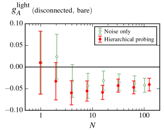
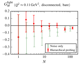
Figure 2: Comparison of hierarchical probing to the “Noise only” method at equal computational cost, using a reduced set of 366 configurations where we have data from both methods. The plots show results for the disconnected light-quark $g_{A}$ (left) and disconnected light-quark magnetic form factor $G_{M}(Q^{2}\approx 0.11\>\>{\rm GeV}^{2})$ (right) from the ratio method at $T/a=10$, $\tau/a=5$. The results are plotted as a function of $N$, which denotes the number of noise samples or the number of Hadamard vectors used to estimate each quark loop. Data points (slightly offset horizontally for clarity) are shown for $N=1,2,4,8,16,32,64$ (both methods), $N=100$ (noise only), and $N=128$ (hierarchical probing).

II.5 Excited-state effects

It turns out that the different form factors suffer from quite different amounts of excited-state contamination. In addition, the available $(T,\tau)$ combinations are quite different between our connected-diagrams data and our disconnected-diagrams data. In particular, the former are much better suited for applying the summation method than the latter. Therefore we choose the best method for isolating the ground state separately for each form factor. We do this by examining “plateau” plots where, for each $(T,\tau)$ we determine “effective” form factors from the ratios assuming the absence of excited states. In a region where excited-state effects are negligible, these effective form factors will form a stable plateau. In addition to these plateaus from the ratio method, we also show results from the summation method, taking the sums with three adjacent points $\{T,T+2a,T+4a\}$ and fitting with a line to determine the slope.

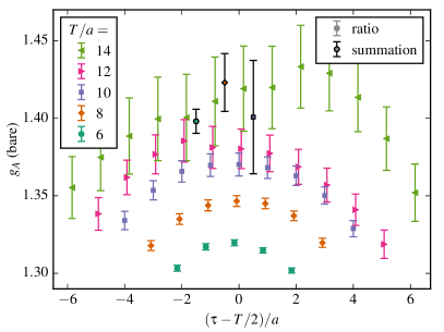
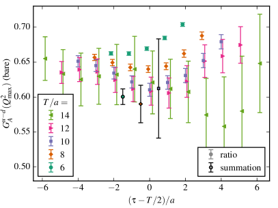
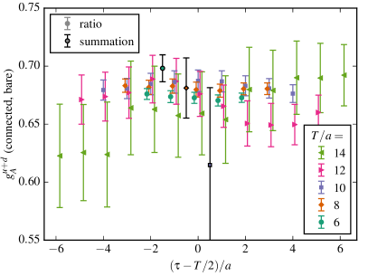
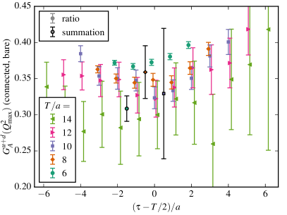
Figure 3: Plateau plots for the bare isovector (top row) and connected isoscalar (bottom row) axial form factors at zero (left column) and the highest (right column) momentum transfer $Q^{2}$. Solid symbols indicate data computed using the ratio method. Symbols with black outlines and black error bars indicate data from the summation method and are plotted in open spaces between ratio data near the origin for clarity.

Figure 3 (top row) shows plateau plots for the isovector axial form factor $G_{A}^{u-d}(Q^{2})$. For the axial charge $g_{A}\equiv G_{A}^{u-d}(0)$ (top left), the centers of the plateaus appear stable by $T/a=10$ and 12, which agree within uncertainty. The center of the plateau for the largest source-sink separation, $T=14a$, is shifted significantly higher, however its statistical uncertainty is quite large and the magnitude of the shift goes against expectations: in the asymptotic regime, as $T$ is increased the shift between neighboring values of $T$ is expected to decrease. Therefore we conclude that the shift at $T=14a$ is likely a statistical fluctuation and take the results from $T=12a$ as the best option using the ratio method. For the summation method, all three points are consistent within the uncertainty and we conclude that the summation method has reached a plateau already at the shortest source-sink separation, $T=6a$ (i.e., from fitting to the sums with $T/a\in\{6,8,10\}$). We take this as our primary analysis method for the isovector axial form factor $G_{A}^{u-d}(Q^{2})$. For this form factor and for any observable derived from it, we estimate systematic uncertainty due to excited-state effects as the root-mean-square (RMS) deviation between the primary result (summation with $T=6a$) and two alternatives: the ratio method with $T=12a$ and the summation method with $T=8a$. Looking at the corresponding plateau plot (top right) for the isovector axial form factor at our largest momentum transfer (about 1.1 GeV²) indicates that this approach is also reasonable at nonzero $Q^{2}$. The bottom row of the same figure shows the equivalent plots for the contribution from quark-connected diagrams to the isoscalar axial form factor $G_{A}^{u+d}(Q^{2})$. The excited-state effects appear to be slightly milder than for the isovector case, and we thus choose to apply the same analysis strategy.

Figure 4: Plateau plots for the bare disconnected light (top row) and strange (bottom row) axial form factors at zero (left column) and the highest (right column) momentum transfer $Q^{2}$.

Plateau plots for the contributions from quark-disconnected diagrams to axial form factors are shown in Fig. 4. Note that since these form factors were computed for several fixed source-operator separations $\tau$, we choose to use the operator-sink separation $T-\tau$ as the horizontal axis. The top row shows the light-quark case, where we computed disconnected loops for five source-operator separations, and the bottom row shows the strange-quark case where we only computed three source-operator separations. The left and right columns show $Q^{2}=0$ (i.e., the contributions to the nucleon spin) and our largest momentum transfer, respectively. In general, we do not see any significant dependence on $T-\tau$ for $T-\tau\gtrsim 5a$. Since the disconnected data were averaged over the exchange of source and sink momenta, the effective form factors are expected to be symmetric, and therefore this corresponds to a source-sink separation of $T=10a$. We use this for our primary result (averaged over the three points near $\tau=T/2$, which reduces statistical uncertainty), and use the RMS deviation with results from $T=8a$ and $T=12a$ as our estimate of systematic uncertainty due to excited states.

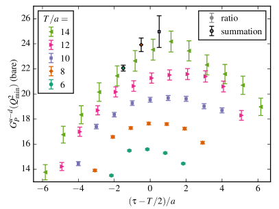
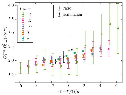
Figure 5: Plateau plots for the bare isovector induced pseudoscalar form factor $G_{P}^{u-d}(Q^{2})$ at the lowest (left) and highest (right) momentum transfer $Q^{2}$. Solid symbols indicate data computed using the ratio method, and symbols with black outlines and black error bars indicate data from the summation method.

The isovector induced pseudoscalar form factor $G_{P}^{u-d}(Q^{2})$ at the lowest available momentum transfer (about 0.1 GeV²) is shown in Fig. 5 (left). This has very large excited-state effects (there is nearly a factor of two between the smallest and largest value on the plot), and there is no sign that a plateau has been reached using the ratio method. For the summation method, the points with $T/a=8$ and 10 are consistent, suggesting that a plateau might possibly have been reached. We take the summation method with $T=8a$ as our primary analysis method for this form factor and estimate the systematic uncertainty as the RMS deviation between the primary result and those from the ratio method with $T/a=14$ and 12. Although the latter is clearly not in the plateau regime, we nevertheless include it in order to reflect the poor control over excited-state effects that is available in our data. At larger $Q^{2}$ (right), the excited-state effects are much milder and our error estimate should be conservative.

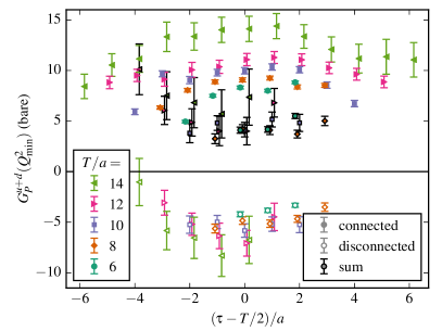
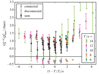
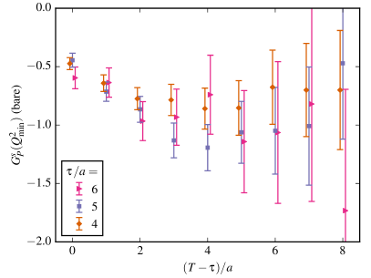
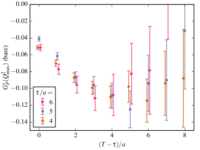
Figure 6: Plateau plots for the bare isoscalar light (top row) and strange (bottom row) induced pseudoscalar form factors at the lowest (left) and highest (right) momentum transfer $Q^{2}$. In the top row: solid and open symbols indicate the contributions from connected and disconnected diagrams, respectively, and symbols with black outlines and black error bars indicate their sum.

Plateau plots for the light and strange isoscalar induced pseudoscalar form factors are shown in Fig. 6. For $G_{P}^{u+d}(Q^{2})$ at the lowest available momentum transfer (top left), we again find that the connected contributions have significant excited-state effects. On the same plot, we show the partial plateaus (limited to the available values of $\tau$) for the contributions from disconnected diagrams. Although they are a bit noisier, they also appear to contain excited-state effects, with the opposite sign. In fact, the opposite signs cause the sum of connected and disconnected diagrams to have smaller excited-state contamination. For the sum, using the ratio method with $T=10a$ appears to be a safe choice, also at the maximum momentum transfer (top right). When we examine the individual connected and disconnected contributions, we will make the same choice, with the understanding that the results include some contamination from excited states, and can only be studied qualitatively. This choice also appears safe for $G_{P}^{s}(Q^{2})$ (bottom left and right). As for the disconnected $G_{A}$ form factors, we use the RMS difference with $T/a=8$ and 12 as our estimate of systematic uncertainty due to excited states.

II.6 Form factor fits using the $z$ expansion

Having computed nucleon form factors at several discrete values of $Q^{2}$, we fit them with curves to characterize their overall shape and determine observables such as the axial radius from their slope at $Q^{2}=0$. It has been common to perform these fits using simple ansatzes, such as a dipole, which is often used to describe experimental data for the isovector $G_{A}(Q^{2})$, however these tend to be highly constrained and introduce a model dependence into the results.

Instead, we use the model-independent $z$ expansion. This was used in Refs. Bhattacharya:2011ah ; Bhattacharya:2015mpa ; Meyer:2016oeg to study axial form factors determined from quasielastic (anti)neutrino-nucleon scattering; it was found that fitting with the $z$ expansion produced a significantly larger axial radius with a larger uncertainty, compared with dipole fits. The $z$ expansion makes use of a conformal mapping from $Q^{2}$, where the given form factor is analytic on the complex plane outside a branch cut on the timelike real axis, to the variable $z$ such that the form factor is analytic for $|z|<1$. We use

$$z(Q^{2})=\frac{\sqrt{t_{\text{cut}}+Q^{2}}-\sqrt{t_{\text{cut}}}}{\sqrt{t_{\text{cut}}+Q^{2}}+\sqrt{t_{\text{cut}}}},$$ (12)

where we use the particle production threshold for the isovector form factors, $t_{\text{cut}}=(3m_{\pi})^{2}$. For the isoscalar form factors the actual threshold may be higher, but we use the same $t_{\text{cut}}$ everywhere for simplicity. We have chosen the mapping such that $Q^{2}=0$ maps to $z=0$.

The $G_{P}$ form factors have an isolated pole below the particle production threshold at the pseudoscalar meson mass, which we remove before fitting. We thus perform fits to

$$G(Q^{2})=\begin{cases}G_{A}(Q^{2})&\\ (Q^{2}+m_{\pi}^{2})G_{P}(Q^{2})&\text{isovector}\\ (Q^{2}+m_{\eta}^{2})G_{P}(Q^{2})&\text{isoscalar}\end{cases}.$$ (13)

Each form factor can be described by a convergent Taylor series in $z$. We truncate this series and obtain our fit form,

$$G(Q^{2})=\sum_{k=0}^{k_{\text{max}}}a_{k}z(Q^{2})^{k}.$$ (14)

The first two coefficients, $a_{0}$ and $a_{1}$, give the intercept and slope of the form factor at $Q^{2}=0$. Specifically, $G(0)=a_{0}$ and, for the axial form factors, $r_{A}^{2}=-3a_{1}/(2a_{0}t_{\text{cut}})$. We impose Gaussian priors on the remaining coefficients, centered at zero with width equal to $w=5\max\{|a_{0}|,|a_{1}|\}$. The series is truncated with $k_{\text{max}}=5$, but this is large enough that increasing it further has no effect in our probed range of $Q^{2}$; i.e., the priors cause $a_{k}z^{k}$ to be negligible for $k>5$.

We perform correlated fits, minimizing

$$\chi^{2}_{\text{aug}}\equiv\sum_{i,j}\left(G(Q^{2}_{i})-\sum_{k}a_{k}z(Q^{2}_{i})^{k}\right)\Xi_{ij}\left(G(Q^{2}_{j})-\sum_{k^{\prime}}a_{k^{\prime}}z(Q^{2}_{j})^{k^{\prime}}\right)+\sum_{k>1}\frac{a_{k}^{2}}{w^{2}}$$ (15)

with respect to $\{a_{k}\}$, where $\Xi$ is an estimator for the inverse covariance matrix and the last term augments the chi-squared with the Gaussian priors. With limited statistics it can be difficult to obtain a reliable estimator, and therefore we choose to reduce statistical fluctuations by interpolating between the jackknife estimate of the covariance matrix and a simplified (less noisy but biased) estimate, and then inverting the resulting matrix. This is in the spirit of shrinkage estimators Ledoit_2004 ; Schaefer_2005 , however we do not perform an optimization step with respect to the interpolation parameter.

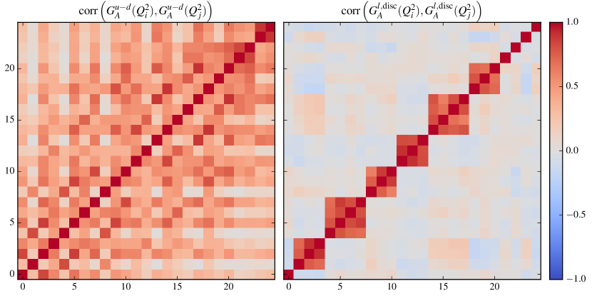
Figure 7: Correlations between data at different $Q^{2}$. Left: the isovector axial form factor $G_{A}^{u-d}(Q^{2})$. Right: the quark-disconnected contribution to the light-quark axial form factor $G_{A}^{l,\text{disc}}(Q^{2})$. The axes index the different momentum transfers, which are sorted in order of increasing $Q^{2}$.

In order to choose the form of the target (simplified) covariance matrix, we examine the correlation matrix

$$R_{ij}\equiv\frac{C_{ij}}{\sqrt{C_{ii}C_{jj}}},$$ (16)

where $C$ is the jackknife estimate of the covariance matrix. We find that this has a quite different form between connected diagrams and disconnected diagrams. Figure 7 shows two example correlation matrices. For connected diagrams, illustrated with $G_{A}^{u-d}(Q^{2})$ (left), we find modest correlations between different values of $Q^{2}$ but no strong pattern. For disconnected diagrams, illustrated with the quark-disconnected contribution to the light-quark $G_{A}$ form factor (right), the correlation matrix is nearly block-diagonal. Each block corresponds to values of $Q^{2}$ that share the same spatial momentum transfer $(\vec{p}\,^{\prime}-\vec{p})^{2}$ and thus the same Fourier modes of the disconnected loops. There are strong correlations within each block but weak correlations between different blocks.

For connected diagrams, we set $\Xi=\left((1-\lambda)C+\lambda C_{\text{diag}}\right)^{-1}$, where $C_{\text{diag}}$ is the diagonal part of the covariance matrix. This is equivalent to multiplying the off-diagonal elements of $C$ by $1-\lambda$. We use the mild value of $\lambda=0.1$ as our main choice. For disconnected diagrams, we compute the average $r$ over all elements of $R_{ij}$ where $i$ and $j$ ($i\neq j$) correspond to the same spatial momentum transfer. We then use for $\Xi$ the inverse of the matrix $R^{\star}_{ij}\sqrt{C_{ii}C_{jj}}$, where

$$R^{\star}_{ij}=\begin{cases}1&i=j\\ (1-\lambda_{1})R_{ij}&\text{$i$ and $j$ have different $(\vec{p}\,^{\prime}-\vec{p})^{2}$}\\ (1-\lambda_{2})R_{ij}+\lambda_{2}r&\text{$i$ and $j$ have the same $(\vec{p}\,^{\prime}-\vec{p})^{2}$}\end{cases}.$$ (17)

As our main choice, we use $(\lambda_{1},\lambda_{2})=(1,\tfrac{1}{2})$.

To estimate systematic uncertainty from fitting, we perform several alternative fits. We halve the value of $w$. For connected diagrams, we perform fits with $\lambda=0$ and 1. For disconnected diagrams, we perform fits with $(\lambda_{1},\lambda_{2})=(0,0)$, $(1,0)$, and $(1,1)$. Finally, we take the RMS difference between results from all of the alternative fits as our estimate.

III Renormalization

To compare our results with phenomenology, the lattice axial current needs to be renormalized. We determine the necessary renormalization factors nonperturbatively using the Rome-Southampton approach Martinelli:1994ty . Going beyond the usual computation of the flavor nonsinglet renormalization factor, we also renormalize the flavor singlet axial current nonperturbatively. This requires disconnected quark loops but we are able to reuse the same loops that were computed for nucleon three-point functions. Since we perform these calculations on just one ensemble without taking the chiral limit, we effectively absorb the mass-dependent operator improvement terms into the renormalization (see Subsec. II.3), which requires us to determine a matrix of renormalization factors.

The singlet-nonsinglet difference in axial renormalization factors has been previously studied nonperturbatively by QCDSF Chambers:2014pea at the $SU(3)$ flavor symmetric point, using additional lattice ensembles and the Feynman-Hellmann relation to determine the contributions from disconnected quark loops. For the case of two degenerate quark flavors, nonperturbative results were presented by RQCD at the Lattice 2016 conference Bali:2017jyw , using stochastic estimation for the disconnected loops similarly to this work. The singlet-nonsinglet difference has also been studied at leading (two-loop) order in lattice perturbation theory for a variety of improved Wilson-type actions Skouroupathis:2008mf ; Constantinou:2016ieh .

This section is organized as follows: we present the Rome-Southampton method and the RI^′-MOM and RI-SMOM schemes for the single-flavor case in Subsec. III.1, determine the light and strange vector current renormalization factors in Subsec. III.2, study discretization effects and breaking of rotational symmetry in Subsec. III.3, and discuss issues of matching to the $\overline{\text{MS}}$ scheme and running of the flavor singlet axial current in Subsec. III.4. Subsections III.5 and III.6 explain our procedure for calculating the $Z_{A}$ renormalization matrix, and finally we give the details of the calculation and its results in Subsec. III.7.

III.1 Rome-Southampton method, RI^′-MOM, and RI-SMOM

For calculating the axial renormalization constants, we follow the Rome-Southampton approach in both RI^′-MOM Martinelli:1994ty ; Gockeler:1998ye and RI-SMOM schemes Sturm:2009kb . In Landau gauge, we compute quark propagators

$$S(p)=\frac{1}{V}\sum_{x,y}e^{-ip(x-y)}\langle q(x)\bar{q}(y)\rangle,$$ (18)

Green’s functions,

$$G_{\mathcal{O}}(p,p^{\prime})=\frac{1}{V}\sum_{x,y,z}e^{-ip^{\prime}.(x-y)-ip.(y-z)}\langle q(x)\mathcal{O}(y)\bar{q}(z)\rangle,$$ (19)

and amputated Green’s functions,

$$\Lambda_{\mathcal{O}}(p,p^{\prime})=S(p^{\prime})^{-1}G_{\mathcal{O}}(p,p^{\prime})S(p)^{-1}.$$ (20)

The renormalized quantities are defined as $S_{R}(p)=Z_{q}S(p)$ and $\Lambda_{\mathcal{O}}^{R}(p,p^{\prime})=Z_{q}^{-1}Z_{\mathcal{O}}\Lambda_{\mathcal{O}}(p,p^{\prime})$. In RI^′-MOM, renormalization conditions are imposed for $p^{\prime}=p$, at scale $p^{2}=p^{\prime 2}=\mu^{2}$. For the quark field and vector and axial currents:

$$\begin{gathered}\lim_{m\to 0}\frac{-i}{12p^{2}}\operatorname{Tr}\left[S_{R}^{-1}(p)\not{p}\right]=1,\\ \lim_{m\to 0}\frac{1}{36}\operatorname{Tr}\left[\Lambda_{V_{\mu}}^{R}(p,p)\left(\gamma_{\mu}-\frac{p_{\mu}\not{p}}{p^{2}}\right)\right]=1,\\ \lim_{m\to 0}\frac{1}{36}\operatorname{Tr}\left[\Lambda_{A_{\mu}}^{R}(p,p)\gamma_{5}\left(\gamma_{\mu}-\frac{p_{\mu}\not{p}}{p^{2}}\right)\right]=1.\end{gathered}$$ (21)

RI-SMOM conditions are imposed at the symmetric point $p^{2}=p^{\prime 2}=q^{2}=\mu^{2}$, where $q=p^{\prime}-p$. The quark-field renormalization is the same as RI^′-MOM, whereas for the vector and axial currents:

$$\begin{gathered}\lim_{m\to 0}\frac{1}{12q^{2}}\operatorname{Tr}\left[q_{\mu}\Lambda_{V_{\mu}}^{R}(p,p^{\prime})\not{q}\right]=1,\\ \lim_{m\to 0}\frac{1}{12q^{2}}\operatorname{Tr}\left[q_{\mu}\Lambda_{A_{\mu}}^{R}(p,p^{\prime})\gamma_{5}\not{q}\right]=1.\end{gathered}$$ (22)

As stated previously, in our calculations we do not take the chiral limit. We also avoid directly determining the quark-field renormalization. Instead, we impose the above renormalization conditions on the vector current, which gives $Z_{q}/Z_{V}$, and independently obtain $Z_{V}$ from three-point functions of pseudoscalar mesons. Our estimate for $Z_{q}$ in RI^′-MOM is then obtained using

$$(Z_{q})_{\text{RI${}^{\prime}$-MOM}}=\frac{Z_{V}}{36}\operatorname{Tr}\left[\Lambda_{V_{\mu}}(p,p)\left(\gamma_{\mu}-\frac{p_{\mu}\not{p}}{p^{2}}\right)\right].$$ (23)

In RI-SMOM, we estimate $Z_{q}$ in the same way using Eq. (22).

The renormalization scale $\mu$ should be chosen such that it is much larger than $\Lambda_{\text{QCD}}$, in order to be able to connect the nonperturbative renormalization schemes to $\overline{\text{MS}}$ using perturbation theory (in our case, this is needed for the flavor-singlet axial current), and much smaller than the inverse lattice spacing to avoid large discretization errors:

$$\Lambda_{\text{QCD}}\ll\mu\ll\pi/a.$$ (24)

As our lattice spacing is fairly coarse, we do not expect to find a stable plateau region in this window. Instead, we will perform fits to remove the leading $O(a^{2}\mu^{2})$ artifacts, and make use of the two different schemes to estimate unaccounted-for systematic uncertainties.

III.2 Vector current renormalization

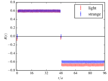
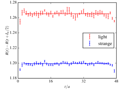
Figure 8: Determination of the vector current renormalization factors. Left: ratio of pseudoscalar three-point to two-point functions. Right: difference of the ratio on opposite sides of the interpolating operator. The horizontal lines indicate the plateau averages.

We obtain the mass-dependent light and strange vector current renormalization factors from matrix elements of pseudoscalar mesons following, e.g., Ref. Durr:2010aw . For $\pi$ and $\eta_{s}$ states, we compute zero-momentum two-point functions $C_{2}(t)$ as well as three-point functions $C_{3}(t)$ with source-sink separation $T=L_{t}/2$ and an operator insertion of the time component of the local (light or strange) vector current at source-operator separation $t$. We form the ratio $R(t)=C_{3}(t)/C_{2}(T)$, so that the charge of the interpolating operator gives the renormalization condition

$$Z_{V}\left(R(t_{1})-R(t_{2})\right)=1,$$ (25)

for $0<t_{1}<T<t_{2}<L_{t}$. Taking the difference $R(t)-R(t+T)$ results in a large cancellation of correlated statistical uncertainties. Results are shown in Fig. 8. We average over the long plateau, excluding three points at each end, and obtain $Z_{V}^{l}=0.7903(2)$ and $Z_{V}^{s}=0.8337(2)$.

III.3 Study of discretization effects

We perform a dedicated study of discretization effects and breaking of rotational symmetry, for the isovector case in the RI^′-MOM scheme. Using translation invariance to remove the sum over $y$ in Eqs. (18) and (19), we compute point-source quark propagators from a fixed point $y$, which allows us to efficiently obtain the gauge-averaged quark propagator and Green’s functions for a large set of momenta. Specifically, we save data for all momenta in the inner 1/16 of the lattice Brillouin zone, i.e., with $|p_{\mu}|\leq\frac{\pi}{2a}$. After checking that the breaking of hypercubic symmetry due to the different lattice temporal and spatial extents is negligible, we averaged the estimates for the isovector $Z_{A}$ over all hypercubic equivalent momenta.

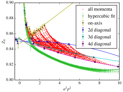
Figure 9: Isovector axial renormalization factor in the RI^′-MOM scheme, computed for all lattice momenta with $|p_{\mu}|\leq\frac{\pi}{2a}$. The raw data for all momenta are shown without error bars to reduce clutter. The points that correspond to momenta that are on-axis or along one of the diagonals are highlighted and shown with error bars, as are the points that result from the hypercubic fit. The curves show the fits that extrapolate $a^{2}p^{2}$ to zero to remove rotationally invariant lattice artifacts, and the points at $a^{2}p^{2}\lesssim 0$ show the results of the extrapolations.

Since the lattice breaks rotational symmetry, estimates of $Z_{A}$ will depend not only on $p^{2}$, but also the hypercubic invariants $p^{[2n]}\equiv\sum_{\mu}(p_{\mu})^{2n}$. We make use of the hypercubic fit form from Refs. Boucaud:2003dx ; Boucaud:2005rm to remove the leading terms that break rotational symmetry and collapse the data to a single function of $p^{2}$:

$$Z_{A}(p^{2},p^{[4]},p^{[6]},\dots)=Z_{A}^{0}(p^{2})+c_{1}\frac{a^{2}p^{[4]}}{p^{2}}+c_{2}\left(\frac{a^{2}p^{[4]}}{p^{2}}\right)^{2}+c_{3}\frac{a^{4}p^{[6]}}{p^{2}}+c_{4}a^{4}p^{[4]}.$$ (26)

The fit parameters are the four $c_{i}$ that control breaking of hypercubic symmetry and a separate $Z_{A}^{0}(p^{2})$ for each $p^{2}$. The data $Z_{A}(p^{2},p^{[4]},\dots)$ and the fit result $Z_{A}^{0}(p^{2})$ are shown in Fig. 9. This is effective at producing a smooth curve that depends only on $p^{2}$ and not the other hypercubic invariants. The resulting curve still contains $O(a^{2}p^{2})$ rotationally invariant lattice artifacts, so we perform a second fit in the range $a^{2}p^{2}\in[2,6]$ assuming a quadratic dependence on $a^{2}p^{2}$, and extrapolate to $a^{2}p^{2}=0$; this is also shown in Fig. 9.

An alternative approach is to pick an initial direction $p_{*}$ and restrict our analysis to points $p=\lambda p_{*}$. Then the hypercubic invariants have the form $p^{[2n]}=c_{2n}p^{2n}$ for some fixed $c_{2n}$ that depend on $p_{*}$. Thus, for this set of points along a fixed direction, the dependence on hypercubic invariants reduces to dependence only on $p^{2}$. We choose four sets of points: on-axis momenta, and momenta along 2, 3, or 4-dimensional diagonals, i.e., $p_{*}=(0,0,0,1)$, $(0,0,1,1)$, $(0,1,1,1)$, and $(1,1,1,1)$. For each set of points, we again do a fit to extrapolate $a^{2}p^{2}$ to zero. Because in this case there are fewer points available, we expand the fit range to be $a^{2}p^{2}\in[1.5,10]$. For on-axis points we use a linear fit because $a^{2}p^{2}$ does not reach very high, and for the $n$-dimensional diagonals we use a quadratic fit. The points from each set and the fit curves are shown in Fig. 9.

We find that the $Z_{A}$ determined from the hypercubic fit and from the fits along different diagonals are all consistent with one another. This indicates that we can reliably control these lattice artifacts by choosing only points along a fixed direction, which is the approach that we will use for our main results for the axial renormalization matrix.

III.4 Matching to $\overline{\text{MS}}$ and running of the singlet axial current

We consider the singlet and nonsinglet axial currents,

$$A_{\mu}^{0}=\frac{1}{\sqrt{N_{f}}}\bar{\psi}\gamma_{\mu}\gamma_{5}\psi,\qquad A_{\mu}^{a}=\bar{\psi}\gamma_{\mu}\gamma_{5}\lambda^{a}\psi,$$ (27)

where $\psi$ is the fermionic field and $\lambda^{a}$ is an $SU(N_{f})$ generator acting in flavor space. The nonsinglet current should be renormalized such that it satisfies the axial Ward identity associated with chiral symmetry, and the renormalized singlet current should satisfy the one-loop form of the axial anomaly. The nonsinglet axial current has no anomalous dimension and is appropriately renormalized to all orders in perturbation theory in $\overline{\text{MS}}$ (using dimensional regularization with a naive anticommuting version of $\gamma_{5}$), RI^′-MOM and RI-SMOM schemes. Thus the matching factor between these schemes is 1, and $Z_{A}=1$ when using a chiral regulator.

For the singlet current, dimensional regularization with a naive $\gamma_{5}$ is inappropriate since the anomaly is not reproduced, and thus the ’t Hooft-Veltman prescription for $\gamma_{5}$ is necessary. Using it in $\overline{\text{MS}}$, an additional finite matching factor $Z_{5}^{s}$ is needed for the renormalized current to satisfy the one-loop form of the axial anomaly Larin:1993tq . Thus renormalized, the singlet current has an anomalous dimension, $\gamma=(\frac{\alpha}{4\pi})^{2}(-6C_{F}N_{f})+O(\alpha^{3})$ Kodaira:1979pa , where the $O(\alpha^{3})$ term is given in Ref. Larin:1993tq . Using the same dimensional regularization, it was shown in Ref. Bhattacharya:2015rsa that the conversion factor between $\overline{\text{MS}}$ (including the finite factor $Z_{5}^{s}$) and RI-SMOM is $1+O(\alpha^{2})$.

For computing the matching between RI^′-MOM and RI-SMOM, at one-loop order there should be no distinction between singlet and nonsinglet currents. Since the matching factor is $1$ for nonsinglet currents, we conclude that the conversion factor for the singlet axial current in RI^′-MOM is $1+O(\alpha^{2})$.

We remove the running of the singlet $Z_{A}$ by evolving to a fixed scale. The evolution is given by

$$\mu^{2}\frac{d}{d\mu^{2}}\ \log\left(Z_{5}^{s}Z_{A}^{\overline{\text{MS}},\text{HV}}\right) =\gamma(\alpha)=-\sum_{i}\gamma_{i}\alpha^{i+1},$$ (28)

$$\mu^{2}\frac{d}{d\mu^{2}}\alpha =\beta(\alpha)=-\sum_{i}\beta_{i}\alpha^{i+2},$$ (29)

where the relevant coefficients are

$$\begin{gathered}\begin{aligned} \beta_{0}&=\frac{1}{4\pi}\;\left(\frac{11}{3}C_{A}-\frac{4}{3}T_{F}N_{f}\right)=\frac{1}{4\pi}\left(11-\frac{2}{3}N_{f}\right),\\ \beta_{1}&=\frac{1}{(4\pi)^{2}}\;\left(\frac{34}{3}C_{A}^{2}-\frac{20}{3}C_{A}T_{F}N_{f}-4C_{F}T_{F}N_{f}\right)=\frac{1}{(4\pi)^{2}}\left(102-\frac{38}{3}N_{f}\right),\\ \gamma_{0}&=0,\\ \gamma_{1}&=\frac{1}{(4\pi)^{2}}(6C_{F}N_{f})=\frac{1}{(4\pi)^{2}}8N_{f},\end{aligned}\end{gathered}$$ (30)

using $C_{A}=3$, $C_{F}=4/3$, and $T_{F}=1/2$. At two-loop order, the evolution of $\alpha$ is given by Prosperi:2006hx :

$$\alpha(\mu)=-\frac{\beta_{0}}{\beta_{1}}\frac{1}{1+W_{-1}(\zeta)},\qquad\zeta=-\frac{\beta_{0}^{2}}{e\beta_{1}}\left(\frac{\Lambda^{2}}{\mu^{2}}\right)^{\beta_{0}^{2}/\beta_{1}},$$ (31)

where $W_{k}$ is the many-valued Lambert function defined by $W_{k}(\zeta)e^{W_{k}(\zeta)}=\zeta$. We use the PDG value, $\Lambda_{3}^{\overline{\text{MS}}}=332(19)$ MeV Olive:2016xmw . Using $\gamma_{0}=0$, the evolution of the renormalization factor at two-loop order is given by

$$\frac{Z(\mu)}{Z(\mu_{0})}=\left(\frac{\beta_{0}+\beta_{1}\alpha(\mu)}{\beta_{0}+\beta_{1}\alpha(\mu_{0})}\right)^{\gamma_{1}/\beta_{1}}.$$ (32)

III.5 Renormalization of the axial current: $N_{f}=2+1$

Consider the flavor-diagonal axial currents, Eq. (27), with $\psi=(u\;d\;s)^{T}$. We take $a=3,8,0,$ with $\operatorname{Tr}(\lambda^{a}\lambda^{b})=\delta^{ab}$,

$$\lambda^{3}=\frac{1}{\sqrt{2}}\begin{pmatrix}1&0&0\\ 0&-1&0\\ 0&0&0\end{pmatrix},\;\lambda^{8}=\frac{1}{\sqrt{6}}\begin{pmatrix}1&0&0\\ 0&1&0\\ 0&0&-2\end{pmatrix},\;\lambda^{0}=\frac{1}{\sqrt{3}}\begin{pmatrix}1&0&0\\ 0&1&0\\ 0&0&1\end{pmatrix}.$$ (33)

Using $i,j$ to label quark flavors, we compute the quark propagator $S_{i}(p)$ [Eq. (18)] for quark flavor-$i$, nonamputated and amputated Green’s functions [Eq. (19), Eq. (20)] for mixed quark flavors-$i$ and -$j$, $G_{i,j}^{\mathcal{O}}(p^{\prime},p)$, and $\Lambda_{ij}^{\mathcal{O}}(p^{\prime},p)$, respectively. These renormalize as

$$\Lambda_{R,ij}^{A_{\mu}^{a}}(p^{\prime},p)=\frac{Z_{A}^{ab}}{\sqrt{Z_{q}^{i}Z_{q}^{j}}}\Lambda_{ij}^{A_{\mu}^{b}}(p^{\prime},p).$$ (34)

For $N_{f}=2+1$, the renormalization pattern is

$$Z_{A}=\begin{pmatrix}Z_{A}^{33}&0&0\\ 0&Z_{A}^{88}&Z_{A}^{80}\\ 0&Z_{A}^{08}&Z_{A}^{00}\end{pmatrix},$$ (35)

and for $N_{f}=3$, this reduces to two independent factors since $Z_{A}^{88}=Z_{A}^{33}$ and $Z_{A}^{80}=Z_{A}^{08}=0$.

In a RI^′-MOM or RI-SMOM scheme, the renormalization condition for $Z_{A}$ involves tracing $\Lambda^{A_{\mu}}$ with some projector $P_{\mu}$ at kinematics corresponding to the scale $\mu^{2}$ (see Subsec. III.1). In the case of multiple flavors, this becomes

$$\sum_{ij}\lambda_{ji}^{a}\operatorname{Tr}\left[\Lambda_{R,ij}^{A_{\mu}^{b}}P_{\mu}\right]_{\mu^{2}}=\delta^{ab},$$ (36)

so that we get

$$(Z_{A}^{-1}(\mu))^{ba}=\sum_{ij}\lambda_{ji}^{a}\operatorname{Tr}\left[\frac{1}{\sqrt{Z_{q}^{i}Z_{q}^{j}}}\Lambda_{ij}^{A_{\mu}^{b}}P_{\mu}\right]_{\mu^{2}}.$$ (37)

Specifically, this yields for $N_{f}=2+1$

$$(Z_{A}^{-1})^{33} =\frac{1}{2Z_{q}^{l}}\operatorname{Tr}\left[\left(\Lambda_{u,u}^{A_{\mu}^{u-d}}-\Lambda_{d,d}^{A_{\mu}^{u-d}}\right)P_{\mu}\right]=\frac{1}{Z_{q}^{l}}\Sigma_{l,\text{conn}},$$ (38)

where $\Sigma_{l,\text{conn}}$ is the connected contribution to the ($u$ or $d$)-quark amputated axial vertex function, traced with $P_{\mu}$. This corresponds to the usual isovector result. Writing $\Sigma_{j,\text{disc}}^{i}$ for the disconnected contribution to the amputated vertex function with the flavor-$i$ axial current and flavor-$j$ external quark states, traced with $P_{\mu}$, we get

$$(Z_{A}^{-1})^{88} =\frac{1}{6}\operatorname{Tr}\left[\left(\frac{1}{Z_{q}^{l}}\Lambda_{u,u}^{A_{\mu}^{u+d-2s}}+\frac{1}{Z_{q}^{l}}\Lambda_{d,d}^{A_{\mu}^{u+d-2s}}-\frac{2}{Z_{q}^{s}}\Lambda_{s,s}^{A_{\mu}^{u+d-2s}}\right)P_{\mu}\right]$$

$$=\frac{1}{3}\left(\frac{1}{Z_{q}^{l}}\Sigma_{l,\text{conn}}+\frac{2}{Z_{q}^{s}}\Sigma_{s,\text{conn}}\right)+\frac{2}{3}\left(\frac{1}{Z_{q}^{l}}\Sigma_{l,\text{disc}}^{l-s}-\frac{1}{Z_{q}^{s}}\Sigma_{s,\text{disc}}^{l-s}\right),$$ (39)

$$(Z_{A}^{-1})^{80} =\frac{1}{3\sqrt{2}}\operatorname{Tr}\left[\left(\frac{1}{Z_{q}^{l}}\Lambda_{u,u}^{A_{\mu}^{u+d-2s}}+\frac{1}{Z_{q}^{l}}\Lambda_{d,d}^{A_{\mu}^{u+d-2s}}+\frac{1}{Z_{q}^{s}}\Lambda_{s,s}^{A_{\mu}^{u+d-2s}}\right)P_{\mu}\right]$$

$$=\frac{\sqrt{2}}{3}\left(\frac{1}{Z_{q}^{l}}\Sigma_{l,\text{conn}}-\frac{1}{Z_{q}^{s}}\Sigma_{s,\text{conn}}\right)+\frac{\sqrt{2}}{3}\left(\frac{2}{Z_{q}^{l}}\Sigma_{l,\text{disc}}^{l-s}+\frac{1}{Z_{q}^{s}}\Sigma_{s,\text{disc}}^{l-s}\right),$$ (40)

$$(Z_{A}^{-1})^{08} =\frac{1}{3\sqrt{2}}\operatorname{Tr}\left[\left(\frac{1}{Z_{q}^{l}}\Lambda_{u,u}^{A_{\mu}^{u+d+s}}+\frac{1}{Z_{q}^{l}}\Lambda_{d,d}^{A_{\mu}^{u+d+s}}-\frac{2}{Z_{q}^{s}}\Lambda_{s,s}^{A_{\mu}^{u+d+s}}\right)P_{\mu}\right]$$

$$=\frac{\sqrt{2}}{3}\left(\frac{1}{Z_{q}^{l}}\Sigma_{l,\text{conn}}-\frac{1}{Z_{q}^{s}}\Sigma_{s,\text{conn}}\right)+\frac{\sqrt{2}}{3}\left(\frac{1}{Z_{q}^{l}}\Sigma_{l,\text{disc}}^{2l+s}-\frac{1}{Z_{q}^{s}}\Sigma_{s,\text{disc}}^{2l+s}\right),$$ (41)

$$(Z_{A}^{-1})^{00} =\frac{1}{3}\operatorname{Tr}\left[\left(\frac{1}{Z_{q}^{l}}\Lambda_{u,u}^{A_{\mu}^{u+d+s}}+\frac{1}{Z_{q}^{l}}\Lambda_{d,d}^{A_{\mu}^{u+d+s}}+\frac{1}{Z_{q}^{s}}\Lambda_{s,s}^{A_{\mu}^{u+d+s}}\right)P_{\mu}\right]$$

$$=\frac{1}{3}\left(\frac{2}{Z_{q}^{l}}\Sigma_{l,\text{conn}}+\frac{1}{Z_{q}^{s}}\Sigma_{s,\text{conn}}\right)+\frac{1}{3}\left(\frac{2}{Z_{q}^{l}}\Sigma_{l,\text{disc}}^{2l+s}+\frac{1}{Z_{q}^{s}}\Sigma_{s,\text{disc}}^{2l+s}\right).$$ (42)

It is clear that $(Z_{A}^{-1})^{80}$ and $(Z_{A}^{-1})^{08}$ vanish when $N_{f}=3$, and the disconnected contribution to $(Z_{A}^{-1})^{88}$ is doubly suppressed by approximate $SU(3)_{f}$ symmetry.

Having evaluated an effective $Z_{A}^{-1}$ in some scheme at a scale $\mu$, we can invert the matrix and evolve to the target scale of 2 GeV:

$$Z_{A}^{8i}(2\text{ GeV})=Z_{A}^{8i}(\mu),\qquad Z_{A}^{0i}(2\text{ GeV})=\left(\frac{Z_{A}^{0}(2\text{ GeV})}{Z_{A}^{0}(\mu)}\right)_{\text{pert}}Z_{A}^{0i}(\mu),$$ (43)

where the perturbative flavor-singlet evolution is given by Eq. (32). Finally, we fit with a polynomial in $a^{2}\mu^{2}$ to remove lattice artifacts. If we want to obtain a single-flavor axial current, such as the strange, we can write, e.g.,

$$A_{\mu}^{R,s} =\frac{1}{\sqrt{3}}A_{\mu}^{R,0}-\sqrt{\frac{2}{3}}A_{\mu}^{R,8}$$

$$=\frac{1}{3}\left(Z_{A}^{00}+2Z_{A}^{88}-\sqrt{2}Z_{A}^{80}-\sqrt{2}Z_{A}^{08}\right)A_{\mu}^{s}+\frac{1}{3}\left(Z_{A}^{00}-Z_{A}^{88}+\frac{1}{\sqrt{2}}Z_{A}^{08}-\sqrt{2}Z_{A}^{80}\right)A_{\mu}^{u+d}$$ (44)

$$\equiv Z_{A}^{s,s}A_{\mu}^{s}+Z_{A}^{s,u+d}A_{\mu}^{u+d}.$$

Similarly, we can evaluate the renormalized $u+d$ current,

$$A_{\mu}^{R,u+d} =\frac{2}{\sqrt{3}}A_{\mu}^{R,0}+\sqrt{\frac{2}{3}}A_{\mu}^{R,8}$$

$$=\frac{1}{3}\left(2Z_{A}^{00}+Z_{A}^{88}+\sqrt{2}Z_{A}^{80}+\sqrt{2}Z_{A}^{08}\right)A_{\mu}^{u+d}+\frac{2}{3}\left(Z_{A}^{00}-Z_{A}^{88}+\frac{1}{\sqrt{2}}Z_{A}^{08}-\sqrt{2}Z_{A}^{80}\right)A_{\mu}^{s}$$ (45)

$$\equiv Z_{A}^{u+d,u+d}A_{\mu}^{u+d}+Z_{A}^{u+d,s}A_{\mu}^{s}.$$

In order to study the disconnected light-quark current by itself, as described in Subsection II.2, we introduce a quenched third light quark $r$, degenerate with $u$ and $d$. Then the connected contribution to the matrix elements of the $u+d$ current is the same as matrix elements of the $u+d-2r$ current. Since this is a nonsinglet flavor combination formed from degenerate light quarks, it has the same renormalization factor as the isovector current. To find the disconnected light-quark contribution, we take the difference,

$$A_{\mu}^{R,l,\text{disc}}=A_{\mu}^{R,r} =\frac{1}{2}(A_{\mu}^{R,u+d}-A_{\mu}^{R,u+d-2r})$$ (46)

$$=\frac{1}{2}(Z_{A}^{u+d,u+d}A_{\mu}^{u+d}+Z_{A}^{u+d,s}A_{\mu}^{s}-Z_{A}^{33}A_{\mu}^{u+d,\text{conn}})$$

$$=Z_{A}^{u+d,u+d}A_{\mu}^{l,\text{disc}}+\frac{1}{2}\left((Z_{A}^{u+d,u+d}-Z_{A}^{33})A_{\mu}^{u+d,\text{conn}}+Z_{A}^{u+d,s}A_{\mu}^{s}\right).$$

III.6 Volume-source approach and reuse of disconnected diagrams

We evaluate our observables using quark propagators with four-dimensional volume plane-wave sources $D_{q}^{-1}(x|p)\equiv\sum_{y}D_{q}^{-1}(x,y)e^{ipy}$. For a quark-bilinear operator $\mathcal{O}=\bar{q}\Gamma q$ ($\Gamma=\gamma_{\mu}\gamma_{5}$ for the axial current), the connected contribution to the Green’s function is obtained using

$$G_{\mathcal{O},\text{conn}}(p^{\prime},p)=\frac{1}{V}\left\langle\sum_{y}e^{i(p^{\prime}-p)y}\gamma_{5}D_{q}^{-1}(y|p^{\prime})^{\dagger}\gamma_{5}\Gamma D_{q}^{-1}(y|p)\right\rangle_{U},$$ (47)

where $\langle\dots\rangle_{U}$ denotes the average over gauge configurations. We obtain the disconnected contribution by correlating the plane-wave-source propagators with the previously-computed disconnected loops $T_{\mu}^{q}(\vec{k},t)$ [Eq. (8)]:

$$G_{\mathcal{O},\text{disc}}(p^{\prime},p)=\frac{L_{t}}{V}\left\langle\sum_{x}e^{-ip^{\prime}x}D_{q^{\prime}}^{-1}(x|p)e^{ik_{4}t}T_{\mu}^{q}(\vec{0},t)\right\rangle_{U},$$ (48)

where $q$ and $q^{\prime}$ are the quark flavors of the operator and the external quark states, and we choose $p^{\prime}-p=(\vec{0},k_{4})$. Translation invariance implies that this expression is independent of $t$, and we average over all timeslices on which the disconnected loops were computed.

III.7 Results

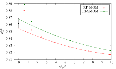
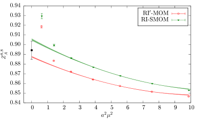
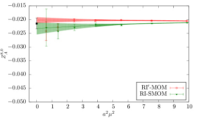
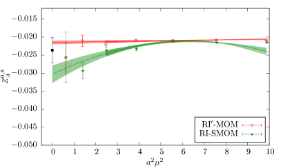
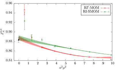
Figure 10: $Z_{A}$ matrix elements for the $\{A_{\mu}^{3},A_{\mu}^{8},A_{\mu}^{0}\}$ basis, in the $\overline{\text{MS}}$ scheme at scale 2 GeV. Each plot shows the data versus the matching point $a^{2}\mu^{2}$ for the two intermediate schemes, as well as an illustrative fit curve for each scheme used to extrapolate to $a^{2}\mu^{2}=0$. The black point at $a^{2}\mu^{2}=0$ shows the value and the combined statistical and systematic uncertainty, based on these and other fits.

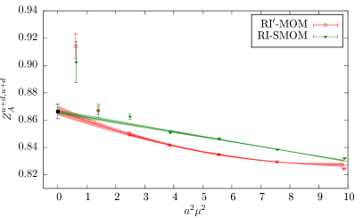
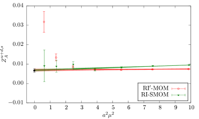
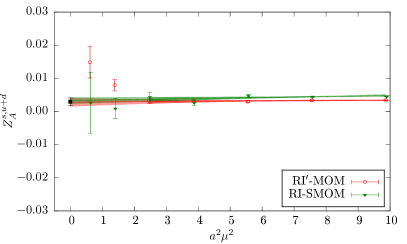
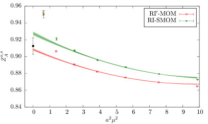
Figure 11: $Z_{A}$ matrix elements for $\{A_{\mu}^{u+d},A_{\mu}^{s}\}$. See the caption of Fig. 10.

In order to minimize cut-off effects we choose momenta on the diagonal of the Brillouin zone $p,p^{\prime}\in\frac{2\pi k}{L_{s}}(1,1,1,\pm 1)$ for $k\in\{2,3,...,8\}$. Therefore, our momenta span the range $0.6<a^{2}\mu^{2}<10$. We used for this calculation about 200 gauge configurations. This procedure involves the following steps:

1. Compute Landau gauge-fixed quark propagators and Green’s functions for both light and strange quarks as outlined in the previous section. Form the amputated vertex functions.

2. On the connected diagrams, impose the RI^′-MOM or RI-SMOM vector current renormalization conditions, together with the renormalization factors from Subsec. III.2, to find estimates for $Z_{q}^{l}$ and $Z_{q}^{s}$ at each scale $\mu$.

3. Trace the axial amputated vertex functions with $P_{\mu}$ to obtain $\Sigma^{l}_{\text{conn}}$, $\Sigma^{s}_{\text{conn}}$, $\Sigma^{l}_{l,\text{disc}}$, $\Sigma^{s}_{l,\text{disc}}$, $\Sigma^{l}_{s,\text{disc}}$, and $\Sigma^{s}_{s,\text{disc}}$ at each scale $|p|$. By combining the different $\Sigma$ following Eqs. (38–42), form the matrix $Z_{A}^{-1}$.

4. Invert the matrix and evolve from scale $\mu$ to 2 GeV.

5. Optionally, convert the $Z_{A}$ matrix from the basis $\{A_{\mu}^{3},A_{\mu}^{8},A_{\mu}^{0}\}$ to $\{A_{\mu}^{u-d},A_{\mu}^{u+d},A_{\mu}^{s}\}$, using Eqs. (44) and (45).

6. Extrapolate $\mu$ to zero to remove $O(a^{2}\mu^{2})$ lattice artifacts.

For estimating the statistical and systematic errors in removing the $O(a^{2}\mu^{2})$ artifacts, we apply linear and quadratic fits for each matrix element, $Z_{A}^{ij}=c_{0}^{ij}+c_{1}^{ij}(a\mu)^{2}$ and $Z_{A}^{ij}=c_{0}^{ij}+c_{1}^{ij}(a\mu)^{2}+c_{2}^{ij}(a\mu)^{4}$. We apply these fits in different ranges of $a^{2}\mu^{2}$, all of which lie within the range $[2.5,10]$, i.e., always excluding the first two points. This fit procedure is applied to results from both RI^′-MOM and RI-SMOM schemes. We take then three best fits in each scheme (yielding six values), average all of them to get the central value and statistical uncertainty, and use the root-mean-square difference between the six values and the average to get the systematic uncertainty. Figures 10 and 11 show illustrative fits for obtaining the matrix elements in the different bases from both RI^′-MOM and RI-SMOM schemes. We obtain the following $Z_{A}$ matrices:

$$\begin{pmatrix}A_{\mu}^{R,3}\\[5.0pt] A_{\mu}^{R,8}\\[5.0pt] A_{\mu}^{R,0}\end{pmatrix}=\begin{pmatrix}0.8623(1)(71)&0&0\\[5.0pt] 0&0.8942(6)(93)&-0.0214(13)(14)\\[5.0pt] 0&-0.0236(1)(33)&0.8832(30)(36)\end{pmatrix}\begin{pmatrix}A_{\mu}^{3}\\[5.0pt] A_{\mu}^{8}\\[5.0pt] A_{\mu}^{0}\end{pmatrix},$$ (49)

$$\begin{pmatrix}A_{\mu}^{R,u-d}\\[5.0pt] A_{\mu}^{R,u+d}\\[5.0pt] A_{\mu}^{R,s}\end{pmatrix}=\begin{pmatrix}0.8623(1)(71)&0&0\\[5.0pt] 0&0.8662(26)(45)&0.0067(8)(5)\\[5.0pt] 0&0.0029(10)(5)&0.9126(11)(98)\end{pmatrix}\begin{pmatrix}A_{\mu}^{u-d}\\[5.0pt] A_{\mu}^{u+d}\\[5.0pt] A_{\mu}^{s}\end{pmatrix}.$$ (50)

Note that these two different matrices were obtained from independent fits to remove $O(a^{2}\mu^{2})$ artifacts, and thus they are not related exactly by Eqs. (44) and (45). For renormalizing our nucleon form factor data, we use the latter matrix. Finally, the contribution from the bare connected light axial current to the renormalized disconnected light axial current depends on the difference $Z_{A}^{u+d,u+d}-Z_{A}^{33}$, as shown in Eq. (46). In order to reduce uncertainties, we computed this difference by itself using the above procedures, and found $Z_{A}^{u+d,u+d}-Z_{A}^{33}=0.0061(18)(10)$.

From Eq. (11) and the full mass-dependent $O(a)$ improvement in Ref. Bhattacharya:2005rb , $Z_{A}^{u+d,s}$ and $Z_{A}^{s,u+d}$ first appear at two-loop order in lattice perturbation theory; since the mass-dependent part is further suppressed by $am_{s}$, it follows that these are largely sensitive to the singlet-nonsinglet difference. These elements are less than one percent of the diagonal ones, indicating a small difference, which is consistent with previous studies. For example, Ref. Chambers:2014pea found a singlet-nonsinglet difference $\bar{Z}_{A}-Z_{A}=0.020(3)$, using a similar lattice action. In the $SU(3)$ flavor limit, this corresponds to $\bar{Z}_{A}-Z_{A}=3Z_{A}^{s,u+d}=\frac{3}{2}Z_{A}^{u+d,s}$, so that those mixing factors are about twice as large as ours.

IV Axial form factors

IV.1 $G_{A}$ form factors

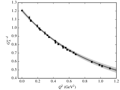
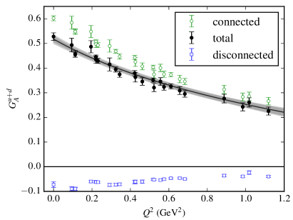
Figure 12: Isovector and light isoscalar axial form factors $G_{A}^{u-d}(Q^{2})$ (left) and $G_{A}^{u+d}(Q^{2})$ (right), and $z$-expansion fits to them. The lattice data and the inner error band for the fit show statistical uncertainties, whereas the outer error band for the fit shows the quadrature sum of statistical and systematic uncertainties. In addition, for the light isoscalar axial form factor, the corresponding form factors from the renormalized connected and disconnected diagrams are also shown.

The isovector axial form factor is shown in Fig. 12 (left). From the fit, we find $g_{A}=1.208(6)(16)(1)(10)$ and $r_{A}^{2}=0.213(6)(13)(3)(0)\text{ fm}^{2}$, where the uncertainties are due to statistics, excited states, fitting, and renormalization, respectively. The dominant uncertainty is excited-state effects. The fitted value of $g_{A}$ is quite compatible with the value taken from the form factor at $Q^{2}=0$, $1.206(7)(19)(0)(10)$, with slightly smaller uncertainties. The axial charge was recently determined in a mostly independent calculation using the same ensemble Yoon:2016jzj , with somewhat higher statistics and different methodology. If we examine the bare quantity to avoid differences in renormalization factors, we get $g_{A}^{\text{bare}}=1.401(7)(18)(2)$, which differs from the result in Ref. Yoon:2016jzj , $g_{A}^{\text{bare}}=1.431(15)$, by slightly more than one standard deviation. We can compare the axial radius with the recent reanalysis of neutrino-deuteron scattering data Meyer:2016oeg that found $r_{A}^{2}=0.46(22)\text{ fm}^{2}$. Our result is slightly more than one standard deviation smaller.

Figure 12 (right) shows the light-quark isoscalar form factor $G_{A}^{u+d}(Q^{2})$. The fit yields $g_{A}^{u+d}=0.517(11)(14)(1)(3)$ and $(r_{A}^{2})^{u+d}=0.197(21)(21)(4)(0)\text{ fm}^{2}$. The statistical errors are relatively much larger than for the isovector case, and the dominant source of these errors is the connected diagrams. The uncertainty due to renormalization in $g_{A}^{u+d}$ is mostly due to the diagonal element of the renormalization matrix; the effect of mixing with strange quarks is very small.

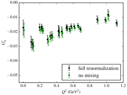
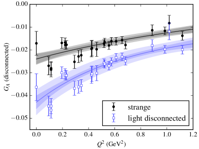
Figure 13: Disconnected axial form factors. Left: strange form factor, both with the full renormalization matrix and after setting the mixing with light quarks to zero. Right: strange and disconnected light-quark axial form factors, including $z$-expansion fits to them. See the caption of Fig. 12.

In Fig. 13 we show the strange and light disconnected axial form factors. The strange axial form factor $G_{A}^{s}(Q^{2})$ is the most important case for mixing between light and strange axial currents, since it is small and it mixes under renormalization with $G_{A}^{u+d}(Q^{2})$, which has a contribution from connected diagrams and is much larger. The effect of this mixing is shown in the left plot: it reduces the magnitude of the form factor by up to 10%, although this effect is smaller than the total statistical uncertainty. In these plots the block-correlated nature of the statistical uncertainties is clearly visible, particularly at low $Q^{2}$: the data that are strongly correlated form clusters of nearby points, but there are large fluctuations between different clusters. This effect was previously seen in the disconnected electromagnetic form factors computed using the same dataset Green:2015wqa . Fits using the $z$ expansion to the strange and light disconnected form factors are shown in the right plot. From these fits we obtain $g_{A}^{s}=-0.0240(21)(8)(2)(7)$ and $g_{A}^{l,\text{disc}}=-0.0430(28)(46)(6)(8)$. The fit has the effect of averaging over several uncorrelated clusters of data, and produces a considerably smaller uncertainty than the value taken directly from the form factor at $Q^{2}=0$. The leading uncertainties are statistical and (for the light-quark case) excited-state effects. The uncertainty due to renormalization is dominated by uncertainty in the off-diagonal part of the renormalization matrix. We also obtain the radii $(r_{A}^{2})^{s}=0.155(73)(57)(7)(2)\text{ fm}^{2}$ and $(r_{A}^{2})^{l,\text{disc}}=0.248(57)(28)(18)(0)\text{ fm}^{2}$. Within their uncertainties, all of the squared axial radii are compatible with 0.2 fm².

IV.2 Quark spin contributions

The axial form factors at zero momentum transfer, $g_{A}^{q}\equiv G_{A}^{q}(0)$, determined in the previous subsection, give the contribution from the spin of quarks $q$ to the proton spin. We can compare against standard experimental inputs used for phenomenological determinations of these quark spin contributions. Using isospin symmetry, the $u-d$ combination is determined from the axial charge in neutron beta decay, $g_{A}^{u-d}=1.2723(23)$ Olive:2016xmw . Our result is about 5% lower, which could be attributed to our heavier-than-physical pion mass.

The flavor nonsinglet combination $u+d-2s$ is typically obtained from semileptonic decays of octet baryons, assuming SU(3) flavor symmetry. Although there have been efforts to improve this determination using chiral perturbation theory (dating back to the original paper on the heavy baryon approach Jenkins:1990jv ), it was shown in Ref. Ledwig:2014rfa that at full next-to-leading order, there is a new low-energy constant that contributes to $g_{A}^{u+d-2s}$ but not to the octet baryon decays. Thus, in the absence of additional input, this combination cannot be predicted at NLO. The leading-order fit to octet baryon decay data Ledwig:2014rfa yields $g_{A}^{u+d-2s}=3F-D=0.608(30)$. It is therefore useful to have a lattice QCD calculation of this quantity, even for a heavy pion mass, since it will enable full NLO chiral perturbation theory analyses to be done. Our result is $g_{A}^{u+d-2s}=0.565(11)(13)$.

$q$	$g_{A}^{q}$
$u$	$0.863(7)(14)$
$d$	$-0.345(6)(9)$
$s$	$-0.0240(21)(11)$

Table 2: Quark spin contributions to the nucleon spin.

We find the total contribution from quark spin to the nucleon spin at $\mu=2$ GeV is $g_{A}^{u+d+s}=0.494(11)(15)$, about half. The other half must come from gluons and from quark orbital angular momentum. This is somewhat larger than results from phenomenological determinations of polarized parton distribution functions: recent analyses deFlorian:2009vb ; Nocera:2014gqa ; Sato:2016tuz give values from 0.18 to 0.28, with an uncertainty ranging from 0.04 to 0.21. There are a few possible sources for this discrepancy. First, that this is caused by our heavier-than-physical pion mass. This would require that the flavor singlet axial case be more sensitive than the isovector one to the pion mass. Second, that the unaccounted-for systematic uncertainties at this pion mass are large. These include effects due to finite lattice spacing and $O(\alpha^{2})$ corrections to the matching of the flavor singlet axial current to $\overline{\text{MS}}$. In particular, the latter does not affect the flavor nonsinglet combinations, which are in better agreement with phenomenology. A third possibility is that the phenomenological values are incorrect. The behavior at small momentum fraction $x$ is poorly constrained, and a recent estimate Kovchegov:2016weo in the large-$N_{c}$ limit of the small-$x$ asymptotics suggests that improved results at small $x$ would lead to higher values of $g_{A}^{u+d+s}$.

The individual quark contributions are summarized in Tab. 2. Our result for $g_{A}^{s}$ is compared with other lattice QCD results in Fig. 14. The results are all mutually consistent, and ours is the most precise. Our improved precision is due to much higher statistics than most previous calculations, as well as the use of a large volume and the additional constraints from data at nonzero $Q^{2}$ in the $z$-expansion fits. We also note the calculation at the physical pion mass by ETMC that was presented at Lattice 2016 Alexandrou:2016tuo , which found $g_{A}^{s}=-0.042(10)$. This differs from our result by almost two standard deviations, suggesting that the strange spin contribution to the nucleon spin becomes larger (more negative) as the light quark mass is decreased.

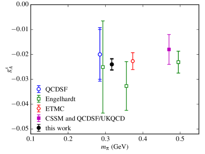
Figure 14: Lattice QCD values for $g_{A}^{s}$ QCDSF:2011aa ; Engelhardt:2012gd ; Abdel-Rehim:2013wlz ; Chambers:2015bka , keeping only peer-reviewed results that use dynamical fermions and nonperturbative renormalization for at least the nonsinglet $Z_{A}$.

IV.3 $G_{P}$ form factors

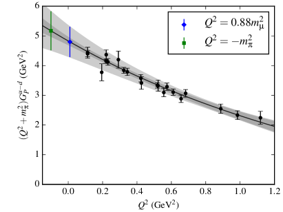
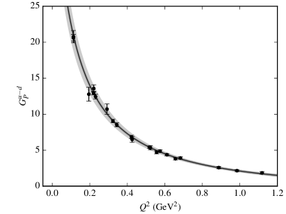
Figure 15: Isovector induced pseudoscalar form factor $G_{P}^{u-d}(Q^{2})$ and the $z$-expansion fit to it. The left plot shows the form factor with the pion pole removed (which is directly fitted using the $z$ expansion), and the right plot has the pole restored in the fit curve. The left plot also shows the extrapolations needed to obtain $g_{P}^{\text{norm}}$ and $g_{\pi NN}$. See the caption of Fig. 12.

Figure 15 shows the isovector induced pseudoscalar form factor $G_{P}^{u-d}(Q^{2})$. As discussed in Subsection II.6, we remove the pion pole that is present in this form factor before fitting using the $z$ expansion. With the pion pole removed, the dependence on $Q^{2}$ is much weaker. At low $Q^{2}$, there is a large systematic uncertainty from excited-state contributions. For comparison with experiment, we consider ordinary muon capture of muonic hydrogen, which (assuming isospin symmetry) is sensitive to $g_{P}^{*}\equiv\frac{m_{\mu}}{2m_{N}}G_{P}^{u-d}(Q_{*}^{2})$, where $Q_{*}^{2}=0.88m_{\mu}^{2}$. To remove the strong dependence on the pion mass arising from the pion pole, we consider Aoki:2010xg

$$g_{P}^{\text{norm}}\equiv\frac{m_{\mu}}{2m_{N}}\frac{Q_{*}^{2}+m_{\pi}^{2}}{Q_{*}^{2}+m_{\pi,\text{phys}}^{2}}G_{P}^{u-d}(Q_{*}^{2})\xrightarrow{m_{\pi}\to m_{\pi,\text{phys}}}g_{P}^{*}.$$ (51)

Using a modest extrapolation of our fit, we find $g_{P}^{\text{norm}}=8.47(21)(87)(2)(7)$, which is consistent with the measurement by the MuCap experiment Andreev:2012fj , $g_{P}^{*}=8.06(55)$. We can also determine the residue of the pion pole: this is related to the pion decay constant $F_{\pi}$ and the pion-nucleon coupling constant $g_{\pi NN}$ Goldberger:1958vp ,

$$\lim_{Q^{2}\to-m_{\pi}^{2}}(Q^{2}+m_{\pi}^{2})G_{P}^{u-d}(Q^{2})=4m_{N}F_{\pi}g_{\pi NN}.$$ (52)

The required extrapolation in $Q^{2}$ is about twice as far as was required for $g_{P}^{*}$, but is still small compared with our probed range of $Q^{2}$. Using $F_{\pi}=106$ MeV computed on this ensemble, we obtain $g_{\pi NN}=11.5(4)(1.4)(1)(0)$. This is slightly more than one standard deviation below the recent result Baru:2010xn determined using pion-nucleon scattering lengths from measurements of pionic atoms: $g_{\pi NN}^{2}/(4\pi)=13.69(20)$, or $g_{\pi NN}=13.12(10)$. In the chiral limit, the pion-nucleon coupling constant is related to the axial charge via the Goldberger-Treiman relation, $g_{\pi NN}=g_{A}^{u-d}m_{N}/F_{\pi}$; on our ensemble the right hand side equals 12.1, and thus our precision is insufficient to resolve a nonzero Goldberger-Treiman discrepancy.

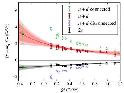
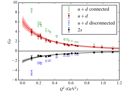
Figure 16: Light and strange isoscalar induced pseudoscalar form factors $G_{P}^{u+d}(Q^{2})$ and $G_{P}^{s}(Q^{2})$ and the $z$-expansion fits to them. In addition, for the light isoscalar form factor, the corresponding form factors for the renormalized connected and disconnected diagrams are also shown. The left plot shows the form factors with the eta pole removed (which is directly fitted using the $z$ expansion), and the right plot has the pole restored in the fit curves. The left plot also shows the extrapolations to the eta pole. See the caption of Fig. 12.

The isoscalar induced pseudoscalar form factors are shown in Fig. 16. As these contain an eta pole, we again remove the pole before fitting with the $z$ expansion. The eta mass is estimated using the leading-order relation from partially quenched chiral perturbation theory, $m_{\eta}^{2}=(m_{\pi}^{2}+2m_{\eta_{s}}^{2})/3$, yielding $m_{\eta}\approx 578$ MeV. Relative to the connected diagrams, the contributions from disconnected diagrams are not small, which is in contrast with what we saw for the $G_{A}$ form factors. This can be understood by considering the partially quenched theory, under which the connected contributions to $G_{P}^{u+d}(Q^{2})$ are equal to $G_{P}^{u+d-2r}(Q^{2})$, where $r$ is a third valence light quark, degenerate with $u$ and $d$. We would expect that this form factor has a pseudoscalar pole from the $\pi_{8}$ meson (which is part of the octet of pseudo-Goldstone bosons under the exact $SU(3)$ symmetry of the valence $u$, $d$, and $r$ quarks) at $Q^{2}=-m_{\pi}^{2}$. The sharp rise of this form factor at low $Q^{2}$ is consistent with this expectation. Since the physical isoscalar form factor does not contain a pole at $Q^{2}=-m_{\pi}^{2}$, the pole must be canceled by the disconnected diagrams, which explains why the disconnected contribution to $G_{P}^{u+d}$ must also rise sharply (with opposite sign) at low $Q^{2}$. Similarly, the expectation that the octet axial current $A_{\mu}^{8}$ couples more strongly than the singlet current $A_{\mu}^{0}$ to the eta meson suggests that $G_{P}^{s}$ and $G_{P}^{u+d}$ should have opposite sign, as seen in the data.

We can attempt to quantify the couplings to the eta meson by studying the generalization of Eq. (52):

$$\lim_{Q^{2}\to-m_{\eta}^{2}}(Q^{2}+m_{\eta}^{2})G_{P}^{a}(Q^{2})=2m_{N}f_{\eta}^{a}g_{\eta NN},$$ (53)

where the eta decay constants are defined by $\langle 0|A_{\mu}^{a}|\eta(p)\rangle=f_{\eta}^{a}p_{\mu}$ Feldmann:1998vh . As Fig. 16 shows, the extrapolation to the eta pole is rather difficult and the results have a large uncertainty. Since we have not separately computed the eta decay constants on this ensemble, we cannot determine the eta-nucleon coupling constant in this way. However, we can take the singlet-octet ratio $f_{\eta}^{0}/f_{\eta}^{8}$, which we find to be $0.96(16)(21)(4)(1)$. This is larger than expected, and three standard deviations above the value obtained from the phenomenological parameters in Ref. Feldmann:1998vh , $f_{\eta}^{0}/f_{\eta}^{8}=0.16(3)$. In particular, since our pion mass is heavier than physical, we would expect the reduced breaking of flavor $SU(3)$ symmetry to yield a value closer to zero. This unexpected behavior is likely caused by the difficulty in such a large extrapolation in $Q^{2}$; direct calculations of these decay constants such as in Ref. Michael:2013vba are much more reliable since they do not require a kinematical extrapolation. If we ignore this issue, and assume the $SU(3)$ relation $f_{\eta}^{8}=f_{\pi}^{3}$, then from $G_{P}^{8}\equiv(G_{P}^{u+d}-2G_{P}^{s})/\sqrt{6}$ we obtain an estimate for the eta-nucleon coupling constant, $g_{\eta NN}=5.2(1.0)(1.0)(0.2)(0)$.

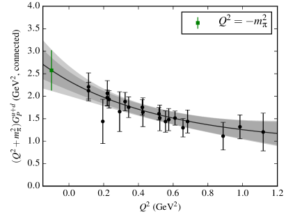
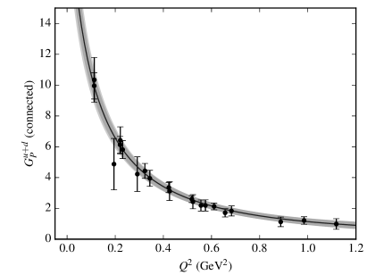
Figure 17: Connected light isoscalar induced pseudoscalar form factor $G_{P}^{u+d,\text{conn}}(Q^{2})$ and the $z$-expansion fit to it. See the caption of Fig. 15.

Assuming flavor $SU(3)$ symmetry, the eta-nucleon coupling constant can also be obtained from the connected contribution to $G_{P}^{u+d}$. Provided that the considerations from the partially quenched theory are valid, the residue of the pion pole is proportional to $F_{\pi}g_{\pi_{8}NN}$, where the $\pi_{8}$-nucleon coupling constant is equal (up to $SU(3)$ breaking corrections) to $g_{\eta NN}$. Alone, the connected contribution does not benefit from the cancellation of excited-state effects with the disconnected contribution that we have seen. Therefore, to better control these effects, we determine this form factor using the summation method in the same way as $G_{P}^{u-d}$; this is shown in Fig. 17. We obtain $g_{\pi_{8}NN}=3.29(35)(45)(3)(0)$. The eta-nucleon coupling constant is not so well known phenomenologically, but both of these estimates are compatible with the value obtained using a generalized Goldberger-Treiman relation, $g_{\eta NN}=3.4(5)$ Feldmann:1999uf .

V Discussion and conclusions

As with our previous study of electromagnetic form factors Green:2015wqa , our approach of using hierarchical probing for disconnected loops and high statistics for nucleon two-point functions is effective at producing a good signal for disconnected nucleon axial form factors. In contrast with the previous study, however, we find that the gauge noise is dominant over the noise from stochastic estimation of the loops, so that further improvements in the latter would be of limited value.

A useful feature of disconnected loops is that they can be reused for calculating many different observables. We did this for computing the axial renormalization factors nonperturbatively, and we were again able to obtain a reasonable signal. At the scale $\mu=2$ GeV, the effect of mixing between light and strange axial currents is small: $G_{A}^{s}(Q^{2})$, which is most affected, is reduced in magnitude by up to 10%. The accuracy of our renormalization is limited by the unknown $O(\alpha^{2})$ term in the matching of the flavor singlet axial current to the $\overline{\text{MS}}$ scheme. Our use of two different intermediate schemes may provide some estimate of this term, but it is possible that the effect in converting between the two intermediate schemes is smaller than in converting to $\overline{\text{MS}}$. A smaller flavor-singlet renormalization factor would make both $g_{A}^{u+d+s}$ and $f_{\eta}^{0}/f_{\eta}^{8}$ more consistent with expectations. This highlights the need for higher-order conversion factors. In the flavor-nonsinglet case, these factors have been computed up to three-loop order for some operators Gracey:2003yr ; Gracey:2006zr . As lattice calculations of disconnected diagrams have made great progress, there is now a need for similar matching calculations in the flavor-singlet sector.

Since this work was performed using only one lattice ensemble, we do not provide an estimate of systematic uncertainties due to the heavier-than-physical pion mass or due to discretization effects. The former have been investigated in many lattice calculations of the isovector axial charge, where generally only modest effects have been seen. Generalizing this, we don’t expect large dependence on the pion mass for $G_{A}^{q}(Q^{2})$. On the other hand, the $G_{P}$ form factors — especially the isovector one — will have a significant dependence on light quark masses due to the presence of pseudoscalar poles. Discretization effects for this lattice ensemble have been studied in Ref. Yoon:2016jzj , where it is compared with another ensemble with similar pion mass and smaller lattice spacing. The isovector axial charge computed on the two ensembles is consistent within one standard deviation, or about 3%, which gives a rough estimate of uncertainty due to finite lattice spacing. We expect that these effects are of similar size for other nucleon matrix elements involving the axial current.

We found that the statistical correlations between the values of a form factor at different $Q^{2}$ behave differently for connected and disconnected diagrams. In the latter case, data with different spatial momentum transfers are nearly uncorrelated. This has the result of better constraining fits to the form factors; using these fits, we were able to obtain a precise value for the strange axial charge on our ensemble, $g_{A}^{s}=-0.0240(21)(11)$, which is consistent with previous lattice calculations.

For $G_{A}(Q^{2})$, the disconnected diagrams are small compared with the connected ones. For instance, $g_{A}^{u+d,\text{disc}}/g_{A}^{u+d}=-0.17$, and the strange disconnected diagrams are about half as large as the light ones. However, this is somewhat larger than we saw for the electromagnetic form factors Green:2015wqa , where the disconnected light magnetic moment, $\mu^{u+d,\text{disc}}\approx 0.11$, is about 4% of the full experimental value $\mu^{u+d}=3(\mu^{p}+\mu^{n})\approx 2.6$, and the disconnected $G_{E}(Q^{2})$ is even smaller relative to the full experimental form factor. This may change closer to the physical pion mass, since the disconnected light-quark matrix elements are expected to grow as the quark mass is decreased.

For $G_{P}(Q^{2})$, the situation is different, with disconnected diagrams not nearly as suppressed. This can be understood from the dominant influence of the pseudoscalar poles in these form factors, which leads to a significant cancellation between the connected and disconnected contributions to $G_{P}^{u+d}(Q^{2})$. As the pion mass is decreased toward the physical point, we expect that $G_{P}^{u+d}(Q^{2})$ will vary only mildly, but at low $Q^{2}$ the individual connected and disconnected contributions will become much larger since the location of the pion pole will approach $Q^{2}=0$. This growing cancellation may make it difficult to obtain a good signal for the full form factor at the physical pion mass and low $Q^{2}$.

*

Appendix A Form factor fit parameters

In this appendix we give parameters for the form factor fits and the estimated total uncertainty. Recall that we performed fits of the form

$$G(Q^{2})=\sum_{k=0}^{5}a_{k}z(Q^{2})^{k},$$ (54)

where $z(Q^{2})$ is given in Eq. (12), $t_{\text{cut}}=(3m_{\pi})^{2}$, and we used the central value $am_{\pi}=0.1833$. The parameters are given in Tab. 3, where for each fit we have also given the correlation matrix. For the $G_{P}$ form factors, we give parameters for fits to $G(Q^{2})=a^{2}(Q^{2}+m^{2})G_{P}(Q^{2})$, where $m$ is either $m_{\pi}$ or $m_{\eta}$; we used the value $am_{\eta}=0.3342$. The fit curves and outer error bands for the physical form factors shown in Sec. IV (i.e., excluding the individual connected and disconnected parts) can be reproduced using the data in this table.

$G_{A}^{u-d}(Q^{2})$
k	$a_{k}$	Correlation matrix
0	$1.208(20)$	$1$	$-0.771$	$0.365$	$-0.101$	$0.067$	$0.058$
1	$-3.985(332)$		$1$	$-0.767$	$0.509$	$0.229$	$0.168$
2	$0.877(1.639)$			$1$	$-0.911$	$-0.471$	$-0.299$
3	$7.730(4.783)$				$1$	$0.416$	$0.201$
4	$4.324(3.101)$					$1$	$0.963$
5	$1.615(1.417)$						$1$
$G_{A}^{u+d}(Q^{2})$
k	$a_{k}$	Correlation matrix
0	$0.517(18)$	$1$	$-0.712$	$0.430$	$-0.215$	$-0.271$	$-0.323$
1	$-1.582(274)$		$1$	$-0.821$	$0.427$	$0.459$	$0.467$
2	$0.947(1.975)$			$1$	$-0.822$	$-0.826$	$-0.803$
3	$-0.853(5.519)$				$1$	$0.990$	$0.965$
4	$-0.534(2.451)$					$1$	$0.991$
5	$-0.214(745)$						$1$
$G_{A}^{s}(Q^{2})$
k	$a_{k}$	Correlation matrix
0	$-0.0240(24)$	$1$	$-0.678$	$0.478$	$0.314$	$0.177$	$0.094$
1	$0.0577(386)$		$1$	$-0.943$	$-0.802$	$-0.656$	$-0.575$
2	$0.0274(1445)$			$1$	$0.845$	$0.687$	$0.598$
3	$-0.0079(507)$				$1$	$0.963$	$0.911$
4	$-0.0049(156)$					$1$	$0.987$
5	$-0.0017(43)$						$1$
$a^{2}(Q^{2}+m_{\pi}^{2})G_{P}^{u-d}(Q^{2})$
k	$a_{k}$	Correlation matrix
0	$1.613(174)$	$1$	$-0.882$	$0.518$	$0.052$	$0.056$	$0.107$
1	$-3.997(1.583)$		$1$	$-0.838$	$0.086$	$0.118$	$0.078$
2	$-3.946(5.729)$			$1$	$-0.365$	$-0.423$	$-0.403$
3	$4.078(5.339)$				$1$	$0.991$	$0.974$
4	$1.825(2.345)$					$1$	$0.994$
5	$0.506(675)$						$1$
$a^{2}(Q^{2}+m_{\eta}^{2})G_{P}^{u+d}(Q^{2})$
k	$a_{k}$	Correlation matrix
0	$0.690(128)$	$1$	$-0.948$	$0.815$	$0.305$	$0.074$	$-0.022$
1	$-2.805(1.929)$		$1$	$-0.941$	$-0.194$	$0.071$	$0.174$
2	$3.790(6.441)$			$1$	$0.200$	$-0.083$	$-0.192$
3	$0.829(3.428)$				$1$	$0.957$	$0.909$
4	$0.045(1.336)$					$1$	$0.990$
5	$-0.031(360)$						$1$
$a^{2}(Q^{2}+m_{\eta}^{2})G_{P}^{s}(Q^{2})$
k	$a_{k}$	Correlation matrix
0	$-0.121(17)$	$1$	$-0.868$	$0.664$	$0.719$	$0.714$	$0.689$
1	$0.256(223)$		$1$	$-0.935$	$-0.909$	$-0.838$	$-0.765$
2	$0.538(766)$			$1$	$0.949$	$0.858$	$0.771$
3	$0.191(293)$				$1$	$0.976$	$0.931$
4	$0.049(83)$					$1$	$0.988$
5	$0.011(20)$						$1$

Table 3: Parameters for the $z$-expansion fits, along with their correlation matrices. The latter are symmetric, and we have omitted redundant entries.

References

- (1) M. Burkardt, “Impact parameter space interpretation for generalized parton distributions,” Int. J. Mod. Phys. A 18 (2003) 173–208, arXiv:hep-ph/0207047.
- (2) European Muon Collaboration, J. Ashman et al., “A measurement of the spin asymmetry and determination of the structure function in deep inelastic muon-proton scattering,” Phys. Lett. B 206 (1988) 364.
- (3) V. Bernard, L. Elouadrhiri, and U.-G. Meißner, “Axial structure of the nucleon,” J. Phys. G 28 (2002) R1–R35, arXiv:hep-ph/0107088.
- (4) J. Green, S. Meinel, M. Engelhardt, S. Krieg, J. Laeuchli, J. Negele, K. Orginos, A. Pochinsky, and S. Syritsyn, “High-precision calculation of the strange nucleon electromagnetic form factors,” Phys. Rev. D 92 (2015) 031501, arXiv:1505.01803 [hep-lat].
- (5) V. Papavassiliou, “Strangeness in the nucleon, cold dark matter in the universe, and neutrino scattering off liquid argon,” AIP Conf. Proc. 1222 (2010) 186–190.
- (6) S. Güsken, “A Study of smearing techniques for hadron correlation functions,” Nucl. Phys. Proc. Suppl. 17 (1990) 361–364.
- (7) APE Collaboration, M. Albanese, F. Costantini, G. Fiorentini, F. Fiore, M. P. Lombardo, et al., “Glueball masses and string tension in lattice QCD,” Phys. Lett. B 192 (1987) 163–169.
- (8) J. R. Green, J. W. Negele, A. V. Pochinsky, S. N. Syritsyn, M. Engelhardt, et al., “Nucleon electromagnetic form factors from lattice QCD using a nearly physical pion mass,” Phys. Rev. D 90 (2014) 074507, arXiv:1404.4029 [hep-lat].
- (9) S. Capitani, B. Knippschild, M. Della Morte, and H. Wittig, “Systematic errors in extracting nucleon properties from lattice QCD,” PoS LATTICE2010 (2010) 147, arXiv:1011.1358 [hep-lat].
- (10) ALPHA Collaboration, J. Bulava, M. A. Donnellan, and R. Sommer, “The coupling in the static limit,” PoS LATTICE2010 (2010) 303, arXiv:1011.4393 [hep-lat].
- (11) S. N. Syritsyn, J. D. Bratt, M. F. Lin, H. B. Meyer, J. W. Negele, et al., “Nucleon electromagnetic form factors from lattice QCD using 2+1 flavor domain wall fermions on fine lattices and chiral perturbation theory,” Phys. Rev. D 81 (2010) 034507, arXiv:0907.4194 [hep-lat].
- (12) LHPC and SESAM Collaboration, P. Hägler et al., “Moments of nucleon generalized parton distributions in lattice QCD,” Phys. Rev. D 68 (2003) 034505, arXiv:hep-lat/0304018.
- (13) G. Martinelli and C. T. Sachrajda, “A lattice study of nucleon structure,” Nucl. Phys. B 316 (1989) 355.
- (14) W. Wilcox, “Noise methods for flavor singlet quantities,” in Numerical Challenges in Lattice Quantum Chromodynamics, A. Frommer, T. Lippert, B. Medeke, and K. Schilling, eds., vol. 15 of Lecture Notes in Computational Science and Engineering, pp. 127–141. Springer Berlin Heidelberg, 2000. arXiv:hep-lat/9911013.
- (15) J. Foley, K. Jimmy Juge, A. O’Cais, M. Peardon, S. M. Ryan, et al., “Practical all-to-all propagators for lattice QCD,” Comput. Phys. Commun. 172 (2005) 145–162, arXiv:hep-lat/0505023.
- (16) A. Stathopoulos, J. Laeuchli, and K. Orginos, “Hierarchical probing for estimating the trace of the matrix inverse on toroidal lattices,” SIAM J. Sci. Comput. 35(5) (2013) S299–S322, arXiv:1302.4018 [hep-lat].
- (17) C. W. Bernard and M. F. L. Golterman, “Partially quenched gauge theories and an application to staggered fermions,” Phys. Rev. D 49 (1994) 486–494, arXiv:hep-lat/9306005.
- (18) C. Bernard and M. Golterman, “On the foundations of partially quenched chiral perturbation theory,” Phys. Rev. D 88 (2013) 014004, arXiv:1304.1948 [hep-lat].
- (19) HPQCD Collaboration, R. J. Dowdall et al., “The Upsilon spectrum and the determination of the lattice spacing from lattice QCD including charm quarks in the sea,” Phys. Rev. D 85 (2012) 054509, arXiv:1110.6887 [hep-lat].
- (20) T. Bhattacharya, R. Gupta, W. Lee, S. R. Sharpe, and J. M. S. Wu, “Improved bilinears in lattice QCD with non-degenerate quarks,” Phys. Rev. D 73 (2006) 034504, arXiv:hep-lat/0511014.
- (21) J. Green, M. Engelhardt, S. Krieg, S. Meinel, J. Negele, A. Pochinsky, and S. Syritsyn, “Nucleon form factors with light Wilson quarks,” PoS LATTICE2013 (2014) 276, arXiv:1310.7043 [hep-lat].
- (22) B. Bhattacharya, R. J. Hill, and G. Paz, “Model independent determination of the axial mass parameter in quasielastic neutrino-nucleon scattering,” Phys. Rev. D 84 (2011) 073006, arXiv:1108.0423 [hep-ph].
- (23) B. Bhattacharya, G. Paz, and A. J. Tropiano, “Model-independent determination of the axial mass parameter in quasielastic antineutrino-nucleon scattering,” Phys. Rev. D 92 (2015) 113011, arXiv:1510.05652 [hep-ph].
- (24) A. S. Meyer, M. Betancourt, R. Gran, and R. J. Hill, “Deuterium target data for precision neutrino-nucleus cross sections,” Phys. Rev. D 93 (2016) 113015, arXiv:1603.03048 [hep-ph].
- (25) O. Ledoit and M. Wolf, “A well-conditioned estimator for large-dimensional covariance matrices,” Journal of Multivariate Analysis 88 no. 2, (2004) 365–411.
- (26) J. Schäfer and K. Strimmer, “A shrinkage approach to large-scale covariance matrix estimation and implications for functional genomics,” Statistical Applications in Genetics and Molecular Biology 4 no. 1, (2005) .
- (27) G. Martinelli, C. Pittori, C. T. Sachrajda, M. Testa, and A. Vladikas, “A General method for nonperturbative renormalization of lattice operators,” Nucl. Phys. B 445 (1995) 81–108, arXiv:hep-lat/9411010 [hep-lat].
- (28) QCDSF Collaboration, A. J. Chambers, R. Horsley, Y. Nakamura, H. Perlt, P. E. L. Rakow, G. Schierholz, A. Schiller, and J. M. Zanotti, “A novel approach to nonperturbative renormalization of singlet and nonsinglet lattice operators,” Phys. Lett. B 740 (2015) 30–35, arXiv:1410.3078 [hep-lat].
- (29) G. S. Bali, S. Collins, M. Göckeler, S. Piemonte, and A. Sternbeck, “Non-perturbative renormalization of flavor singlet quark bilinear operators in lattice QCD,” PoS LATTICE2016 (2016) 187, arXiv:1703.03745 [hep-lat].
- (30) A. Skouroupathis and H. Panagopoulos, “Two-loop renormalization of vector, axial-vector and tensor fermion bilinears on the lattice,” Phys. Rev. D 79 (2009) 094508, arXiv:0811.4264 [hep-lat].
- (31) M. Constantinou, M. Hadjiantonis, H. Panagopoulos, and G. Spanoudes, “Singlet versus nonsinglet perturbative renormalization of fermion bilinears,” Phys. Rev. D 94 (2016) 114513, arXiv:1610.06744 [hep-lat].
- (32) M. Göckeler, R. Horsley, H. Oelrich, H. Perlt, D. Petters, P. E. L. Rakow, A. Schäfer, G. Schierholz, and A. Schiller, “Nonperturbative renormalization of composite operators in lattice QCD,” Nucl. Phys. B 544 (1999) 699–733, arXiv:hep-lat/9807044.
- (33) C. Sturm, Y. Aoki, N. H. Christ, T. Izubuchi, C. T. C. Sachrajda, and A. Soni, “Renormalization of quark bilinear operators in a momentum-subtraction scheme with a nonexceptional subtraction point,” Phys. Rev. D 80 (2009) 014501, arXiv:0901.2599 [hep-ph].
- (34) S. Dürr, Z. Fodor, C. Hoelbling, S. D. Katz, S. Krieg, T. Kurth, L. Lellouch, T. Lippert, K. K. Szabó, and G. Vulvert, “Lattice QCD at the physical point: Simulation and analysis details,” JHEP 08 (2011) 148, arXiv:1011.2711 [hep-lat].
- (35) P. Boucaud, F. de Soto, J. P. Leroy, A. Le Yaouanc, J. Micheli, H. Moutarde, O. Pène, and J. Rodríguez-Quintero, “Quark propagator and vertex: Systematic corrections of hypercubic artifacts from lattice simulations,” Phys. Lett. B 575 (2003) 256–267, arXiv:hep-lat/0307026.
- (36) P. Boucaud, F. de Soto, J. P. Leroy, A. Le Yaouanc, J. Micheli, H. Moutarde, O. Pène, and J. Rodríguez-Quintero, “Artifacts and power corrections: Reexamining and in the momentum-subtraction scheme,” Phys. Rev. D 74 (2006) 034505, arXiv:hep-lat/0504017.
- (37) S. A. Larin, “The Renormalization of the axial anomaly in dimensional regularization,” Phys. Lett. B 303 (1993) 113–118, arXiv:hep-ph/9302240.
- (38) J. Kodaira, “QCD higher order effects in polarized electroproduction: Flavor singlet coefficient functions,” Nucl. Phys. B 165 (1980) 129–140.
- (39) T. Bhattacharya, V. Cirigliano, R. Gupta, E. Mereghetti, and B. Yoon, “Dimension-5 CP-odd operators: QCD mixing and renormalization,” Phys. Rev. D 92 (2015) 114026, arXiv:1502.07325 [hep-ph].
- (40) G. M. Prosperi, M. Raciti, and C. Simolo, “On the running coupling constant in QCD,” Prog. Part. Nucl. Phys. 58 (2007) 387–438, arXiv:hep-ph/0607209.
- (41) Particle Data Group Collaboration, C. Patrignani et al., “Review of particle physics,” Chin. Phys. C 40 (2016) 100001.
- (42) B. Yoon et al., “Isovector charges of the nucleon from 2+1-flavor QCD with clover fermions,” Phys. Rev. D 95 (2017) 074508, arXiv:1611.07452 [hep-lat].
- (43) E. E. Jenkins and A. V. Manohar, “Baryon chiral perturbation theory using a heavy fermion Lagrangian,” Phys. Lett. B 255 (1991) 558–562.
- (44) T. Ledwig, J. Martin Camalich, L. S. Geng, and M. J. Vicente Vacas, “Octet-baryon axial-vector charges and SU(3)-breaking effects in the semileptonic hyperon decays,” Phys. Rev. D 90 (2014) 054502, arXiv:1405.5456 [hep-ph].
- (45) D. de Florian, R. Sassot, M. Stratmann, and W. Vogelsang, “Extraction of spin-dependent parton densities and their uncertainties,” Phys. Rev. D 80 (2009) 034030, arXiv:0904.3821 [hep-ph].
- (46) NNPDF Collaboration, E. R. Nocera, R. D. Ball, S. Forte, G. Ridolfi, and J. Rojo, “A first unbiased global determination of polarized PDFs and their uncertainties,” Nucl. Phys. B 887 (2014) 276–308, arXiv:1406.5539 [hep-ph].
- (47) Jefferson Lab Angular Momentum Collaboration, N. Sato, W. Melnitchouk, S. E. Kuhn, J. J. Ethier, and A. Accardi, “Iterative Monte Carlo analysis of spin-dependent parton distributions,” Phys. Rev. D 93 (2016) 074005, arXiv:1601.07782 [hep-ph].
- (48) Y. V. Kovchegov, D. Pitonyak, and M. D. Sievert, “Small- asymptotics of the quark helicity distribution,” Phys. Rev. Lett. 118 (2017) 052001, arXiv:1610.06188 [hep-ph].
- (49) C. Alexandrou, M. Constantinou, K. Hadjiyiannakou, C. Kallidonis, G. Koutsou, K. Jansen, C. Wiese, and A. V. Avilés-Casco, “Nucleon spin and quark content at the physical point,” PoS LATTICE2016 (2016) 153, arXiv:1611.09163 [hep-lat].
- (50) QCDSF Collaboration, G. S. Bali, S. Collins, M. Göckeler, R. Horsley, Y. Nakamura, A. Nobile, D. Pleiter, P. E. L. Rakow, A. Schäfer, G. Schierholz, and J. M. Zanotti, “Strangeness contribution to the proton spin from lattice QCD,” Phys. Rev. Lett. 108 (2012) 222001, arXiv:1112.3354 [hep-lat].
- (51) M. Engelhardt, “Strange quark contributions to nucleon mass and spin from lattice QCD,” Phys. Rev. D 86 (2012) 114510, arXiv:1210.0025 [hep-lat].
- (52) A. Abdel-Rehim, C. Alexandrou, M. Constantinou, V. Drach, K. Hadjiyiannakou, K. Jansen, G. Koutsou, and A. Vaquero, “Disconnected quark loop contributions to nucleon observables in lattice QCD,” Phys. Rev. D 89 (2014) 034501, arXiv:1310.6339 [hep-lat].
- (53) A. J. Chambers, R. Horsley, Y. Nakamura, H. Perlt, D. Pleiter, P. E. L. Rakow, G. Schierholz, A. Schiller, H. Stüben, R. D. Young, and J. M. Zanotti, “Disconnected contributions to the spin of the nucleon,” Phys. Rev. D 92 (2015) 114517, arXiv:1508.06856 [hep-lat].
- (54) Y. Aoki, T. Blum, H.-W. Lin, S. Ohta, S. Sasaki, R. Tweedie, J. Zanotti, and T. Yamazaki, “Nucleon isovector structure functions in (2+1)-flavor QCD with domain wall fermions,” Phys. Rev. D 82 (2010) 014501, arXiv:1003.3387 [hep-lat].
- (55) MuCap Collaboration, V. A. Andreev et al., “Measurement of muon capture on the proton to 1% precision and determination of the pseudoscalar coupling ,” Phys. Rev. Lett. 110 (2013) 012504, arXiv:1210.6545 [nucl-ex].
- (56) M. L. Goldberger and S. B. Treiman, “Form factors in decay and capture,” Phys. Rev. 111 (1958) 354–361.
- (57) V. Baru, C. Hanhart, M. Hoferichter, B. Kubis, A. Nogga, and D. R. Phillips, “Precision calculation of the scattering length and its impact on threshold scattering,” Phys. Lett. B 694 (2011) 473–477, arXiv:1003.4444 [nucl-th].
- (58) K.-F. Liu, “Flavor singlet axial charge of the nucleon and anomalous Ward identity,” Phys. Lett. B 281 (1992) 141–147.
- (59) T. Feldmann, P. Kroll, and B. Stech, “Mixing and decay constants of pseudoscalar mesons,” Phys. Rev. D 58 (1998) 114006, arXiv:hep-ph/9802409 [hep-ph].
- (60) European Twisted Mass Collaboration, C. Michael, K. Ottnad, and C. Urbach, “ and masses and decay constants from lattice QCD with quark flavours,” PoS LATTICE2013 (2014) 253, arXiv:1311.5490 [hep-lat].
- (61) T. Feldmann, “Quark structure of pseudoscalar mesons,” Int. J. Mod. Phys. A 15 (2000) 159–207, arXiv:hep-ph/9907491.
- (62) J. A. Gracey, “Three loop anomalous dimension of non-singlet quark currents in the RI′ scheme,” Nucl. Phys. B 662 (2003) 247–278, arXiv:hep-ph/0304113.
- (63) J. A. Gracey, “Three loop anomalous dimensions of higher moments of the non-singlet twist-2 Wilson and transversity operators in the and RI′ schemes,” JHEP 10 (2006) 040, arXiv:hep-ph/0609231.
- (64) SciDAC, LHPC, UKQCD Collaboration, R. G. Edwards and B. Joó, “The Chroma software system for lattice QCD,” Nucl. Phys. Proc. Suppl. 140 (2005) 832, arXiv:hep-lat/0409003.
- (65) M. A. Clark, R. Babich, K. Barros, R. C. Brower, and C. Rebbi, “Solving lattice QCD systems of equations using mixed precision solvers on GPUs,” Comput. Phys. Commun. 181 (2010) 1517–1528, arXiv:0911.3191 [hep-lat].
- (66) R. Babich, M. A. Clark, B. Joó, G. Shi, R. C. Brower, and S. Gottlieb, “Scaling lattice QCD beyond 100 GPUs,” in Proceedings of 2011 International Conference for High Performance Computing, Networking, Storage and Analysis, SC ’11, pp. 70:1–70:11. ACM, New York, NY, USA, 2011. arXiv:1109.2935 [hep-lat].
- (67) A. Pochinsky, “Qlua.” https://usqcd.lns.mit.edu/qlua.