Universal spatio-temporal scaling of distortions in a drifting lattice

Abstract

We study the dynamical response to small distortions of a lattice about its uniform state, drifting through a dissipative medium due to an external force, and show, analytically and numerically, that the fluctuations, both transverse and longitudinal to the direction of the drift, exhibit spatiotemporal scaling belonging to the Kardar-Parisi-Zhang universality class. Further, we predict that a colloidal crystal drifting in a constant electric field is linearly stable against distortions and the distortions propagate as underdamped waves.

I Introduction

It is well known from elastic theory that distortions in a crystal at thermal equilibrium propagate as waves with a speed determined by the elastic constants of the lattice Landau and Lifshitz (1965); Martin et al. (1972). The response of a lattice drifting due to an external force through a dissipative medium was first addressed by Lahiri and Ramaswamy (LR) in  Lahiri and Ramaswamy (1997). The linear stability of the lattice was predicted to depend on certain model parameters that govern the strain-dependence of the mobility of the lattice. The role of anharmonic effects and random fluctuations (possibly of nonequilibrium origin) on the macrocscopic nature of steady states, including scaling properties is still unknown. This potentially opens up the possibility that either the anharmonic effects drive the ensuing steady state away from its equilibrium counter part, or leave the system macroscopically indistinguishable from a crystal in equilibrium. In this letter, we address these issues. Specifically, we ask: what is the macroscopic nature of the drifting non-equilibrium state?

The study of drifting lattices began with the work of Crowley in 1971  Crowley (1971) who predicted that an array of particles moving through a viscous fluid is unstable to clumping due to hydrodynamic forces alone, a result he verified experimentally by dropping steel balls into turpentine oil. The role of elastic and Brownian forces on this lattice instability was analysed by Lahiri and Ramaswamy in 1997  Lahiri and Ramaswamy (1997) . A set of continuum equations for the displacement fields of the drifting lattice, constructed using symmetry agruments, showed that the lattice was linearly unstable to clumping, even in the presence of elasticity. The role of nonlinearities and noise on the linear instability was not analysed. Numerical studies of an equivalent lattice-gas model describing the coupled dynamics of concentration and tilt fields showed that the lattice was stable to distortions upto a critical Péclet number at which a nonequilibrium phase transition to a clumped state occured.

In this work, we find that the nonequilibrium steady state of the drifting lattice is phenomenally different from its equilibrium counterpart. We show that small, long wavelength lattice distortions, exhibit spatiotemporal scaling both transverse and longitudinal to the direction of drift of the lattice and establish, analytically and numerically, that the fluctuations display dynamical scaling that belongs to the Kardar-Parisi-Zhang (KPZ) universality class Kardar et al. (1986). As an example of this drifting nonequilibrium state, we analyse the dynamics of distortions in a colloidal crystal drifting in a constant electric field and show that it has a linearly stable state in which long wavelength distortions propagate as under damped waves. The wave speeds and the length scale beyond which these propagating waves can be detected are also calculated in terms of the driving force and the parameters defining their interactions.

II Drifting lattices in disspative media

For a driven, nonequilibrium system such as ours, the equations of motion for the degrees of freedom must be written down directly, by using symmetry arguments. Physically, the equations of motion for the displacement field $\mathbf{u}(\mathbf{r},t)$ of a lattice moving in a frictional medium, ignoring inertia completely, must obey the equation

$$\dot{\mathbf{u}}=\underline{\underline{\mathbf{M}}}(\nabla\mathbf{u}).\,\mathbf{F}_{tot}=\underline{\underline{\mathbf{M}}}(\nabla\mathbf{u}).(\mathbf{F}+\underline{\underline{\mathbf{D}}}\nabla\nabla\mathbf{u}+\bm{\eta})\,.$$ (1)

Here, $\underline{\underline{\mathbf{M}}}$ is the mobility tensor that depends on the local lattice strain, $\mathbf{F}_{tot}$ is the total force consisting of the external driving force $\mathbf{F}$, elastic forces due to lattice distortions $\underline{\underline{\mathbf{D}}}\nabla\nabla\mathbf{u}$ and the random force $\bm{\eta}$ acting on the particle due to the surrounding fluid. The mobility tensor has the form $\underline{\underline{\mathbf{M}}}=\underline{\underline{\mathbf{M_{0}}}}+\underline{\underline{\mathbf{A}}}(\nabla\mathbf{u})+O(\nabla\mathbf{u})^{2})$ where $\underline{\underline{\mathbf{M_{0}}}}$ is the mean mobility of the undistorted lattice, $\underline{\underline{\mathbf{A}}}$ is the first order correction to it due to lattice distortions and the successive terms higher order corrections  Lahiri and Ramaswamy (1997). These terms arise from interactions between particles in the surrounding viscous medium.

For a lattice in the $(x,y)$ plane drifting along the $\hat{z}$ direction the equations of motion for the displacement field $(\mathbf{u}_{\perp},u_{z})$ are isotropic in the transverse ($\perp$ or $(x,y)$ ) plane but not invariant under $z\rightarrow-z$. The equations hence have the form:

$$\mathbf{\dot{u}}_{\perp}=\lambda_{1}\partial_{z}\mathbf{u}_{\perp}+\lambda_{2}\bm{\nabla}_{\perp}u_{z}+D_{1}\bm{\nabla}_{\perp}^{2}\mathbf{u}_{\perp}+D_{3}\partial_{z}^{2}\,\mathbf{u}_{\perp}+$$

$$O(\nabla u\nabla u)+\bm{\eta}_{\perp},$$ (2)

$$\dot{u}_{z}=\lambda_{3}\bm{\nabla}_{\perp}\cdot\mathbf{u}_{\perp}+\lambda_{4}\partial_{z}{u}_{z}+D_{2}\bm{\nabla}_{\perp}^{2}u_{z}+D_{4}\partial_{z}^{2}u_{z}+$$

$$D_{5}\partial_{z}\bm{\nabla}_{\perp}\cdot\mathbf{u}_{\perp}+O(\nabla u\nabla u)+\eta_{z}.$$ (3)

These follow from eq.(1) albeit in the frame of the drifting lattice. The constant term in (1) has hence been omitted. The $\lambda_{i}\,$s are phenomenological parameters arising from the strain dependence of the mobility and depend crucially on the details of the hydrodynamic interaction between particles in the system. They are proportional to the drift speed of the lattice. The $D_{i}\,$s are diffusion constants coming from elastic restoring forces in eq. (1) . $\eta_{\perp}$ and $\eta_{z}$ are Gaussian white noise in the lattice plane and perpendicular to it respectively. There are a total of nine quadratic nonlinearities, $O(\nabla u\nabla u)$ terms, in these equations which arise from the dependence of the $\lambda_{i}\,$s on the local concentration and tilt ($\bm{\nabla_{\perp}}u_{z}$).

In this paper, we work with a simplified version of these equations in one dimension Lahiri and Ramaswamy (1997). The displacement field $\mathbf{u}(\mathbf{r},t)$ of the lattice then has only two components $(u_{x},u_{z})$ and only derivatives in $x$ are considered; those along the direction of drift $\hat{z}$ are averaged out. With this simplification eqs.(2,3) reduce to

$$\dot{u}_{x}=\lambda_{2}\partial_{x}u_{z}+\gamma_{1}\partial_{x}u_{x}\partial_{x}u_{z}+D_{1}\partial_{x}^{2}u_{x}+\eta_{x}\,,\hskip 14.22636pt$$ (4)

$$\dot{u}_{z}=\lambda_{3}\partial_{x}u_{x}+\gamma_{2}(\partial_{x}u_{x})^{2}+\gamma_{3}(\partial_{x}u_{z})^{2}+D_{2}\partial_{x}^{2}u_{z}+\eta_{z}$$ (5)

Only 3 quadratic nonlinearities are allowed by symmetry and only eq.(5) has the KPZ nonlinearity $(\partial_{x}u_{z})^{2}\,$. The equations are coupled at the linear level and can be decoupled, at the linear level, for fields that are appropriate linear combinations of $u_{x},u_{z}$ (see eqs. (12,13)). Equations of this type have been studied extensively in recent years in various contexts (Ferrari et al. (2013); Mendl and Spohn (2013); van Beijeren (2012); Spohn (July 2015, 2016a, 2016b); Das et al. (2001)).

Linearising and Fourier transforming the above equations in space and time, as in Lahiri and Ramaswamy (1997), yields the dispersion relations for the two modes of the system –

$$\omega=\frac{-ik^{2}(D_{1}+D_{2})}{2}\pm\frac{1}{2}\sqrt{4\lambda_{2}\lambda_{3}k^{2}-k^{4}(D_{1}-D_{2})^{2}}$$ (6)

$\omega$ is the frequency and $k$ the wave number of the mode. For long wavelength (small $k$) distortions this implies that the crystal is linearly stable only when $\lambda_{2}\lambda_{3}>0$. Symmetry arguments alone cannot apriori determine whether the lattice is stable as the signs of these parameters depend on the details of the interaction between particles which is system dependent. For a sedimenting lattice the product $\lambda_{2}\lambda_{3}$ was calculated and found to be negative Lahiri and Ramaswamy (1997) implying a linear instability towards clumping. We calculate $\lambda_{2}\lambda_{3}$ for a colloidal crystal drifting due to an applied electric field before we address the effect of nonlinearities.

Figure 1: Schematic diagram to show displacement fields. $\delta$ and $\epsilon$ are the displacements of a particle in $x$ and $z$ direction from its original position.

III Colloidal crystal in an electric field

Consider a 1D lattice of colloidal particles of radius $a$ with lattice spacing $d$ in the $x$ direction and the electric field $\mathbf{E}$ perpendicular to the lattice (as in Fig.1). A single charged colloid drifts in the field with constant velocity, ${\mathbf{V}}=\xi{\mathbf{E}}$, where $\xi$ is its mobility. Its motion results from a complex interplay of electrostatic, hydrodynamic and thermal forces and its mobility depends on various parameters such as the thickness of the electric double layer of small counterions, surface properties, charge density, ion concentration, and lipophilicity of the colloid and the specific properties of counterions and salt ions. There is as yet no expression for the mobility applicable, in general, as a function of these parameters (Ohshima (2006, 2009, 2015); Lizana and Grosberg (2013)). The mobility of a charged sphere, in the thin double layer limit, was first derived by Smoluchowski von Smoluchowski (1921) to be $\xi_{0}=\epsilon\zeta/\bar{\eta}$ where $\epsilon$ and $\bar{\eta}$ are the dielectric permittivity and viscosity of the colloidal solution and $\zeta$ the Zeta potential on the surface of the sphere. For double layers of arbitrary thickness but small $\zeta$, Smoluchowski’s result for the mobility was modified by Henry to $\xi=\xi_{0}f(\kappa a)$ where $\kappa^{-1}$ is the Debye length Henry (1931) and $f(\kappa a)$ Henry’s function which is an increasing function of $\kappa a$ . The mobility of a particle is modified in the presence of other particles due to interactions between them. For two identical spherical particles of radius $a$, the mobility was derived using the method of reflections by Ennis et al  Ennis and White (1997). The electrophoretic velocity of a sphere in the presence of an identical sphere at a distance $d$ is given by

$$\mathbf{V}=\frac{\xi}{4\pi}[A_{\lVert}\mathbf{ee}+A_{\bot}(\mathbf{I}-\mathbf{ee})+(B_{\rVert}\mathbf{ee}+B_{\bot}(\mathbf{I}-\mathbf{ee}))].\mathbf{E}$$ (7)

Here $\mathbf{e}$ is a unit vector along the line joining the two spheres and $\mathbf{I}$ the unit tensor of rank two. $A_{||}$, $A_{\bot}$, $B_{||}$ and $B_{\bot}$ have the form (keeping only the leading order dependence on $d$ ): $A_{||}=1-(\frac{a}{d})^{3}$ , $A_{\bot}=1+\frac{1}{2}(\frac{a}{d})^{3}$ , $B_{||}=(\frac{a}{d})^{3}\frac{L(\kappa a)}{f(\kappa a)}$ and $B_{\bot}=-(\frac{a}{d})^{3}\frac{L(\kappa a)}{2f(\kappa a)}$. The function $L(\kappa a)$ decreases monotonically with $\kappa a$ . The dominant interaction between two particles, as implied by this result, decays as $1/d^{3}$. Both $f(\kappa a)$ and $L(\kappa a)$ tend to 1 as $\kappa a\rightarrow\infty$. In this limit the result for thin diffuse layers is recovered where particles do not interact with each other.

According to (7) a pair of particles at distance $d$ apart (as in Fig.1) move in the $z$ direction with speed $v_{0}$ given by eq.(7) . If one of them is displaced by $\delta$ and $\epsilon$ along and perpendicular, respectively, to the lattice at some instant of time, the change in velocity $\Delta v_{x}$ and $\Delta v_{z}$ along the $x$ and $z$ directions due to the displacement are

$$\Delta v_{x} = C\left[\frac{3}{2}(\frac{\epsilon}{d})-6(\frac{\delta}{d})(\frac{\epsilon}{d})\right],$$ (8)

$$\Delta v_{z} = C\left[\frac{3}{2}(\frac{\delta}{d})-3(\frac{\delta}{d})^{2}+\frac{9}{4}(\frac{\epsilon}{d})^{2}\right],$$ (9)

where $C\approx v_{0}(\frac{a}{d})^{3}(\frac{L(\kappa a)}{f(\kappa a)}-1)$. Using the expressions for $L(\kappa a)$ and $f(\kappa a)$ from Ennis and White (1997) we find that $L(\kappa a)/f(\kappa a)>1$, for all $\kappa a$ and hence $C>0$. This along with eqns.(9,8) implies that the spheres fall slower when they are closer and a displacement along the field travels in the $+x$ direction. The implications of this for the drifting lattice are evident. A perfect lattice drifts uniformly in the $z$ direction. If the lattice were perturbed, say a region of it compressed, then it would drift slower in this region. With time, this results in a tilt of the interfacial region between the compressed and uncompressed regions. These tilted regions drift laterally as implied by eq.(8). The direction of this lateral drift (given $C>0$) is such that the tilted regions move apart dilating the compressed regions. The lattice is thus stable to distortions. If we approximate $\partial_{x}u_{x}\approx\frac{\delta}{d}$ and $\partial_{x}u_{z}\approx\frac{\epsilon}{d}$, then the expressions on the right hand side (RHS) of eqns. (8,9) are exactly the terms on the RHS of eqns. (4,5). The coefficients $\lambda_{2}$, $\lambda_{3}$ for the drifting lattice can thus be obtained by summing the contributions of the nearest neighbors to the change in velocity $\Delta v_{x}$ and $\Delta v_{z}$ of a particle in the lattice. Our results for two particles allow us to conclude that $\lambda_{2}\lambda_{3}>0$ since $C$ is always greater than zero. The speed of the propagating modes $v\propto\sqrt{\lambda_{2}\lambda_{3}}\approx C$. For particles of radius $a=1\mu m$, $\kappa a=2.5$, $d=3a$ in an electric field of strength $150$ V$/m$, we estimate the speed of the propagating modes to be $~{}10\mu m/s$. These propagating modes dominate beyond a lengthscale $l_{c}\sim 2\pi D/\sqrt{\lambda_{2}\lambda_{3}}$. We estimate $l_{c}\approx 50\,d$ for this system. It should hence be possible to detect these modes in systems that are larger than $l_{c}$. A similar analysis for a 1D lattice drifting parallel to the electric field indicates that the lattice is linearly stable. This is a general result applicable to all drifting lattices. Having established that the lattice is linearly stable, we ask what the effect of the noninearities and noise are on this stable state.

IV Nonlinearities and fluctuations

To analyze the effect of nonlinearities and fluctuations on the linearly stable state, approximate methods must be used as eqns. (4-5) cannot be solved in closed form. Exact results pertaining to their spatial and temporal scaling behavior can be obtained using a dynamic renormalization group (DRG) analysis Barabasi and Stanley (1995); Halpin-Healy and Zhang (1995). In particular, the roughness exponents $\chi_{x},\chi_{z}$ and dynamic exponents $z_{x},z_{z}$ of the fields $u_{x}$ and $u_{z}$, respectively, defined by the scaling forms of their correlation functions

$$C^{xx}(x,t)=\langle u_{x}(x,t)u_{x}(0,0)\rangle=A_{x}|x|^{2\chi_{x}}f_{x}(x/t^{z_{x}}),$$ (10)

$$C^{zz}(x,t)=\langle u_{z}(x,t)u_{z}(0,0)\rangle=A_{z}|x|^{2\chi_{z}}f_{z}(x/t^{z_{z}}),$$ (11)

can be determined using this method. Here the functions $f_{x},f_{z}$ are dimensionless scaling functions of their arguments, and coefficients $A_{x},A_{z}$ are constants. On scaling space as $x\rightarrow bx$, time as $t\rightarrow b^{z_{i}}t$ and the fields as $u_{i}(x,t)\rightarrow b^{\chi_{i}}\,u_{i}(bx,b^{z_{i}}t)\,,i=x,z$, the correlation functions scale as $C^{xx}(x,t)\rightarrow b^{2\chi_{x}}C^{xx}(bx,b^{z_{x}}t),\,C^{zz}(x,t)\rightarrow b^{2\chi_{z}}C^{zz}(bx,b^{z_{z}}t)$. If $z_{x}=z_{z}$, then the model displays strong dynamic scaling, else weak dynamic scaling Das et al. (2001).

We begin by decoupling eqs. (4,5) at the linear level by defining the fields $\phi_{\pm}=u_{x}\pm\nu u_{z}$ where $\nu=\sqrt{\lambda_{2}/\lambda_{3}}$ . In terms of $\phi_{\pm}$, they become

$$\dot{\phi}_{+}-\frac{\alpha}{2}\partial_{x}\phi_{+}+a_{1}(\partial_{x}\phi_{+})^{2}+b_{1}(\partial_{x}\phi_{-})^{2}+$$

$$c_{1}(\partial_{x}\phi_{+})(\partial_{x}\phi_{-})=D_{+}\partial^{2}_{x}\phi_{+}+\eta_{+}\,,$$ (12)

$$\dot{\phi}_{-}+\frac{\alpha}{2}\partial_{x}\phi_{-}+a_{2}(\partial_{x}\phi_{+})^{2}+b_{2}(\partial_{x}\phi_{-})^{2}+$$

$$c_{2}(\partial_{x}\phi_{+})(\partial_{x}\phi_{-})=D_{-}\partial^{2}_{x}\phi_{-}+\eta_{-}\,.$$ (13)

The co-efficient of the wave term $\frac{\alpha}{2}=\sqrt{\lambda_{2}\lambda_{3}}$, $\eta_{\pm}=\eta_{x}\pm\nu\eta_{z}$ and the co-efficients of nonlinear terms depend on $\lambda_{2}$, $\lambda_{3}$, $\gamma_{1}$, $\gamma_{2}$ and $\gamma_{3}$. The zero-mean Gaussian white noises $\eta_{+},\eta_{-}$ are appropriate linear combinations of the noises $\eta_{x},\eta_{z}$ and have correlations $\langle\eta_{+}(x,t)\eta_{+}(x^{\prime},t^{\prime})\rangle=2A_{1}\delta(x-x^{\prime})\delta(t-t^{\prime})$ and $\langle\eta_{-}(x,t)\eta_{-}(x^{\prime},t^{\prime})\rangle=2A_{2}\delta(x-x^{\prime})\delta(t-t^{\prime})\,$. $D_{+}$ and $D_{-}$ are the new diffusion constants. Noises $\eta_{+}$, $\eta_{-}$ have non-zero cross correlations of the form $\langle\eta_{+}(x,t)\eta_{-}(x^{\prime},t^{\prime})\rangle=2A_{3}\delta(x-x^{\prime})\delta(t-t^{\prime})$. Coupled equations of this type have been studied in considerable detail earlier. We refer the reader to the work in (Ferrari et al. (2013); Mendl and Spohn (2013); van Beijeren (2012); Spohn (July 2015, 2016a, 2016b)) for a perspective on this. Our approach here is to use dynamic renormalisation group to extract the scaling properties of these equations. For the special case with $\gamma_{1}=2\gamma_{3}$ and $\gamma_{2}/\gamma_{3}=\lambda_{3}/\lambda_{2}$ Eqs. (12-13) reduce to two separate KPZ equations  Lahiri and Ramaswamy (1997).

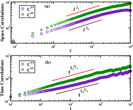
Figure 2: (color online). Log-log plot of equal-time correlators $C^{xx}(l,t=0)$ and $C^{zz}(l,t=0)$ versus spatial separation $l$ (top) and (b) log-log plots of equal space-point time-dependent correlators $C^{xx}(l=0,t)$ and $C^{zz}(l=0,t)$ (bottom) versus $t$. Slopes yield exponents $\chi_{x},\chi_{z}$ and $\chi_{x}/z_{x},\chi_{z}/z_{z}$, respectively (see text).

Fluctuations of $\phi_{+}$ and $\phi_{-}$ propagate with a relative speed between them, thus one can eliminate the linear propagating term in either (12) or (13), but not simultaneously in both. At the linear level, the dynamics of $\phi_{+}$ and $\phi_{-}$ are mutually decoupled. This implies $\chi_{+}=1/2=\chi_{-}$ and $z_{+}=2=z_{-}$, for the roughness and dynamic exponents defined by the correlation functions for $\phi_{+}$ and $\phi_{-}$, analogous to (10-11). This implies $\chi_{x}=1/2=\chi_{z}$ and $z_{x}=2=z_{z}$ in the linear theory.

With the nonlinear terms, eqs. (12,13), cannot be solved exactly and naive perturbative expansions in powers of the nonlinear coefficients yield diverging corrections in the long wavelength limit. In order to deal with these long wavelength divergences in a systematic manner, we employ perturbative one-loop Wilson momentum shell DRG Barabasi and Stanley (1995); Halpin-Healy and Zhang (1995). This is implemented by first integrating out the dynamical fields $\phi_{\pm}({\bf{q}},\omega)$ with wavevector $\Lambda/b<q<\Lambda,\,b>1$, perturbatively up to the one-loop order using (12-13).$\,\Lambda$ is the wave vector upper cut-off. We then rescale wavevectors by $q^{\prime}=bq$, so that the upper cutoff is restored to $\Lambda$. The frequency $\omega$ and the fields are also scaled appropriately Barabasi and Stanley (1995); Halpin-Healy and Zhang (1995).

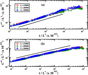
Figure 3: (color online). Log-log plots of $C^{xx}$ (top) and $C^{zz}$ (bottom) as functions of $t/L^{z}$, showing data collapse on to single curves after scaling.

The one-loop perturbation theory is constructed using the bare propagators and correlators of $\phi_{\pm}$. We work in the co-moving frame of $\phi_{+}$ where the bare propagators (in Fourier space) are of the form $G_{0}^{+}(k,\omega)=\frac{1}{D_{+}k^{2}+i\omega}$ and $G_{0}^{-}(k,\omega)=\frac{1}{D_{-}k^{2}+i(\omega-\alpha k)}$, for $\phi_{+}$ and $\phi_{-}$ respectively. Thus, at linear order $\phi_{+}(k,\omega)=G^{+}(k,\omega)\eta_{+}(k,\omega)$ and $\phi_{-}(k,\omega)=G^{-}(k,\omega)\eta_{-}(k,\omega)$. In a similar manner, correlators of $\phi_{\pm}$ in the co-moving frame of $\phi_{+}$ are defined as $C_{\phi_{+}\phi_{+}}(k,\omega)=\frac{2A_{1}}{\omega^{2}+D_{+}^{2}k^{4}}$ and $C_{\phi_{-}\phi_{-}}(k,\omega)=\frac{2A_{2}}{(\omega-\alpha k)^{2}+D_{-}^{2}k^{4}}$. Notice that since each of (12, 13) can be reduced to the standard KPZ equation Kardar et al. (1986) upon setting appropriate coupling constants to zero, the lowest order perturbative corrections to $D_{\pm},A_{1},A_{2},a_{1}$ and $a_{2}$ can clearly be classified into two categories: (i) KPZ-type, which survive in the KPZ limit, and (ii) non-KPZ type, which vanish in that limit. The KPZ-type diagrams are formally identical to those in the pure KPZ problem Kardar et al. (1986). The relevant one-loop Feynman diagrams are listed in the appendix. Retaining only the dominant contributions (all of which arise from the respective KPZ-type diagrams), we find the corrections to be

$$\tilde{A}_{1} =A_{1}\left[1+\frac{a_{1}^{2}A_{1}}{\pi D_{+}^{3}}\int_{\Lambda/b}^{\Lambda}\frac{1}{q^{2}}dq\right],$$ (14)

$$\tilde{A}_{2} =A_{2}\left[1+\frac{A_{1}^{2}a_{2}^{2}}{\pi A_{2}D_{+}^{3}}\int_{\Lambda/b}^{\Lambda}\frac{1}{q^{2}}dq\right],$$ (15)

$$\tilde{D}_{+} =D_{+}\left[1+\frac{A_{1}a_{1}^{2}}{\pi D_{+}^{3}}\int_{\Lambda/b}^{\Lambda}\frac{k^{2}}{q^{2}}dq\right],$$ (16)

$$\tilde{D}_{-} =D_{-}\left[1+\frac{A_{1}a_{2}c_{1}}{\pi 2D_{+}^{2}D_{-}}\int_{\Lambda/b}^{\Lambda}\frac{k^{2}}{q^{2}}dq\right].$$ (17)

None of the vertices $a_{1}$, $b_{1}$, $c_{1}$, $a_{2}$, $b_{2}$ and $c_{2}$ receive any fluctuation corrections at the one-loop order Forster et al. (1977). Under scalings $x\rightarrow bx$, $t\rightarrow b^{z}t$, $\phi_{+}\rightarrow b^{\chi_{+}}\phi_{+}$ and $\phi_{-}\rightarrow b^{\chi_{-}}\phi_{-}$, the parameters scale as $A_{1}\rightarrow b^{z-1-2\chi_{+}}A_{1}$, $A_{2}\rightarrow b^{z-1-2\chi_{-}}A_{2}$, $D_{\pm}\rightarrow b^{z-2}D_{\pm}$. On rescaling the momentum cut off and taking the limit $\delta l\rightarrow 0$, we get the recursion relations

$$\frac{dD_{+}}{dl} = D_{+}[z-2+g]\,,$$

$$\frac{dA_{1}}{dl} = A_{1}[z-1-2\chi_{+}+g]\,,$$

$$\frac{dD_{-}}{dl} = D_{-}[z-2+\frac{1}{2}mnrg]\,,$$

$$\frac{dA_{2}}{dl} = A_{2}[z-1-2\chi_{-}+pn^{2}g]\,,$$ (18)

where the coupling constant $g\equiv\frac{A_{1}a_{1}^{2}}{\pi D_{+}^{3}}$ and dimensionless constants $m=\frac{D_{+}}{D_{-}}$, $p=\frac{A_{1}}{A_{2}}$, $n=\frac{a_{2}}{a_{1}}$, and $r=\frac{c_{1}}{a_{1}}$. The renormalized coupling $g$ then obeys

$$\frac{dg}{dl}=g[-2g+1]\,,$$ (19)

giving the stable RG fixed point $g^{*}=1/2$. The scaling exponents can be extracted from the equations $\frac{dD_{+}}{dl}=\frac{dA_{1}}{dl}=\frac{dD_{-}}{dl}=\frac{dA_{2}}{dl}=0$ at the RG fixed point. This gives $z=3/2$ and $\chi_{+}=\chi_{-}=1/2$, which belong to the KPZ universality class. Strong dynamic scaling prevails as the dynamic exponents for both the fields $\phi_{+}$ and $\phi_{-}$ are the same. Since $u_{x}$ and $u_{z}$ can be written as linear combinations of $\phi_{+}$ and $\phi_{-}$, we have $\chi_{x}=\chi_{z}=1/2$ and $z_{x}=z_{z}=3/2$. The presence of propagating modes here is crucial; they render the so-called non-KPZ nonlinearities irrelevant in the long wavelength limit so the model displays KPZ universality.

Having obtained the scaling exponents in the co-moving frame of $\phi_{+}$, we now argue that the values of these exponents are the same in all reference frames connected by the Galilean transformation Forster et al. (1977). Consider the correlation function, $C_{+}(x_{1}-x_{2},t_{1}-t_{2})=\langle\phi_{+}(x_{1},t_{1})\phi_{+}(x_{2},t_{2})\rangle$: under a Galilean transformation, $t_{1,2}\rightarrow t_{1,2},\;x_{1,2}\rightarrow x_{1,2}+{\sf{v}}t$, where $t$ is the time and ${\sf v}$ the Galilean boost. $\,x_{1}-x_{2}$ and $t_{1}-t_{2}$ are unchanged, hence so is $C_{+}$. The scaling exponents are thus the same in all frames connected by Galilean transformations.

The scaling behavior of the displacement fields $u_{x}$ and $u_{z}$ can also be obtained numerically by integrating eqs. (4,5). The correlation functions $C^{xx}(x,t)$ and $C^{zz}(x,t)$ can be calculated from the solutions of these equations. The equations of motion for $u_{x}$ and $u_{z}$ are simulated with diffusion constants $D_{1}\,=\,D_{2}\,=\,1$, wave velocities $\lambda_{2}=0.1$ , $\lambda_{3}=0.2$ , co-efficients of nonlinear terms $\gamma_{1}=1.0$ , $\gamma_{2}=2.0$ and $\gamma_{3}=10.0$ and time step $dt=0.01$ . We simulate a system of $2\times 10^{4}$ particles. Log-log plots of $C^{xx}(x,0)$ and $C^{zz}(x,0)$ are shown in Fig. 2 (top). We obtain $\chi_{x}=0.47\pm 0.01,\,\chi_{z}=0.485\pm 0.015$. Similarly, the log-log plots of $C^{xx}(0,t)$ and $C^{zz}(0,t)$ shown in Fig. 2 (bottom) yield $z_{x}=1.45\pm 0.05,\,z_{z}=1.49\pm 0.06$, which are the same as the dynamic exponent for the KPZ universality class, within error bars. Our numerical results are thus in close agreement with the DRG results. Fig. 3 shows the correlation functions for different system sizes $L$ collapse on each other on scaling $t$ by $L^{z}$ and correlations by $L^{\chi_{i}}$, for $i=x,z\,$. This clearly establishes universal scaling in the model. Technical details of our numerical studies can be found in the SM.

V Conclusions and Outlook

We have shown that a colloidal crystal drifting in an electric field is linearly stable, with long-wavelength lattice distortions propagating as waves. For particles of radius $a=1\mu m$, $\kappa a=2.5$, $d=3a$ in an electric field of strength $150$ V$/m$, we estimate the speed of the propagating modes to be $~{}10\mu m/s$. Using renormalization group methods we establish that, in the drifting steady state, lattice distortions both transverse and longitudinal to the lattice, display strong dynamic scaling with dynamic exponent $3/2$ and belongs to the KPZ universality class. A numerical analysis of the equations for the displacement fields confirm these results.

The notion of universality survives even for driven elastic media. However, unlike equilibrium, this universal behavior is controlled by the drive, displaying 1D KPZ scaling. While extending our analysis to higher dimensions may be nontrivial, we can comment that in higher (D$>$1) dimensions there should be 1 longitudinal and D-1 transverse modes. The presence of propagating waves should make the system anisotropic. Thus, it is unlikely that the fluctuations in higher dimensions belong to the KPZ universality class. We look forward to theoretical attempts in understanding the universal properties of the fluctuations at higher D and experimental tests of our predictions for propagating modes in drifting colloidal cyrstals.

Appendix A Equations of motion and diagrammatic expansions

The equation of motion for $\phi_{\pm}$ are

$$\dot{\phi}_{+}-\frac{\alpha}{2}\partial_{x}\phi_{+}+a_{1}(\partial_{x}\phi_{+})^{2}+b_{1}(\partial_{x}\phi_{-})^{2}+c_{1}(\partial_{x}\phi_{+})(\partial_{x}\phi_{-})=D_{+}\partial^{2}_{x}\phi_{+}+\eta_{+}$$ (20)

$$\dot{\phi}_{-}+\frac{\alpha}{2}\partial_{x}\phi_{-}+a_{2}(\partial_{x}\phi_{+})^{2}+b_{2}(\partial_{x}\phi_{-})^{2}+c_{2}(\partial_{x}\phi_{+})(\partial_{x}\phi_{-})=D_{-}\partial^{2}_{x}\phi_{-}+\eta_{-}.$$ (21)

where the co-efficient of wave term $\frac{\alpha}{2}=\sqrt{\lambda_{2}\lambda_{3}}$, noises are $\eta_{\pm}=f_{x}\pm\sqrt{\frac{\lambda_{2}}{\lambda_{3}}}f_{z}$ and other co-efficients are $a_{1}=-\frac{(\gamma_{1}+\gamma_{3})}{4}\sqrt{\frac{\lambda_{3}}{\lambda_{2}}}-\frac{\gamma_{2}}{4}\sqrt{\frac{\lambda_{2}}{\lambda_{3}}}$, $b_{1}=-\frac{(\gamma_{3}-\gamma_{1})}{4}\sqrt{\frac{\lambda_{3}}{\lambda_{2}}}-\frac{\gamma_{2}}{4}\sqrt{\frac{\lambda_{2}}{\lambda_{3}}}$, $c_{1}=\frac{\gamma_{3}}{2}\sqrt{\frac{\lambda_{3}}{\lambda_{2}}}-\frac{\gamma_{2}}{2}\sqrt{\frac{\lambda_{2}}{\lambda_{3}}}$ and $a_{2}=-b_{1}$, $b_{2}=-a_{1}$ and $c_{2}=-c_{1}$. In the special case with $\gamma_{1}=2\gamma_{3}$ and $\gamma_{2}/\gamma_{3}=\lambda_{3}/\lambda_{2}$ Eqs. (20-21) reduce to two separate KPZ equations Kardar et al. (1986).

$G_{0}^{+}(k,\omega)$ and $G_{0}^{-}(k,\omega)$ are the bare propagators for $\phi_{+}$ and $\phi_{-}$ respectively in the co-moving frame of $\phi_{+}$  and have the form

$$G_{0}^{+}(k,\omega)=\frac{1}{D_{+}k^{2}+i\omega},\hskip 14.22636ptG_{0}^{-}(k,\omega)=\frac{1}{D_{-}k^{2}+i(\omega-\alpha k)}\,.$$ (22)

The correlators of $\phi_{\pm}$ in the Fourier space are defined in the co-moving frame of $\phi_{+}$ as

$$C_{\phi_{+}\phi_{+}}(k,\omega)=\frac{2A_{1}}{\omega^{2}+D_{+}^{2}k^{4}},\hskip 14.22636ptC_{\phi_{-}\phi_{-}}(k,\omega)=\frac{2A_{2}}{(\omega-\alpha k)^{2}+D_{-}^{2}k^{4}}.$$ (23)

Our perturbative Dynamic Renormalization Group (DRG) calculation may be represented diagrammatically Barabasi and Stanley (1995). The symbols, that we use are explained below.

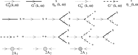
Figure 4: Diagrammatic representation of the propagators and noise for $\phi_{+}$ and $\phi_{-}$. Perturbation expansion for the propagators $G_{+}(k,\omega)$, $G_{-}(k,\omega)$. Contracted noise $A_{1}$, $A_{2}$, $A_{3}$.

Appendix B Propagator renormalization

There are four one-loop diagrams which contribute to the propagator renormalization of $\phi_{\pm}$. Fig. 2  shows the relevant diagrams for propagator renormalization for $\phi_{+}$.

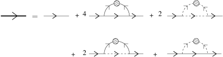
Figure 5: One-loop diagrams for propagator renormalization.

The renormalized propagator $G^{+}(k,\omega)$ can be written as

$$G^{+}(k,\omega)=G_{0}^{+}(k,\omega)+T_{1}+T_{2}+T_{3}+T_{4}$$ (24)

where $T_{1}$ and $T_{2}$ contain contributions only from $\phi_{+}$ and $\phi_{-}$, respectively, and $T_{3}$, $T_{4}$ are the contributions from both the fields. We calculate the individual contributions below.

$$\begin{multlined}T_{1}=\frac{8A_{1}a_{1}^{2}G_{0}^{+}(k,\omega)^{2}}{(2\pi)^{2}}\int dq\int_{-\infty}^{\infty}d\Omega[q(k-q)][-qk]G_{0}^{+}(q,\Omega)G_{0}^{+}(-q,-\Omega)G_{0}^{+}(k-q,\omega-\Omega)\\ =\frac{8A_{1}a_{1}^{2}G_{0}^{+}(k,\omega)^{2}}{(2\pi)^{2}}\int dq\int_{-\infty}^{\infty}d\Omega\frac{[q(k-q)][-qk]}{[D_{+}q^{2}+i\Omega][D_{+}q^{2}-i\Omega][D_{+}(k-q)^{2}-i\Omega]}\\ \end{multlined}T_{1}=\frac{8A_{1}a_{1}^{2}G_{0}^{+}(k,\omega)^{2}}{(2\pi)^{2}}\int dq\int_{-\infty}^{\infty}d\Omega[q(k-q)][-qk]G_{0}^{+}(q,\Omega)G_{0}^{+}(-q,-\Omega)G_{0}^{+}(k-q,\omega-\Omega)\\ =\frac{8A_{1}a_{1}^{2}G_{0}^{+}(k,\omega)^{2}}{(2\pi)^{2}}\int dq\int_{-\infty}^{\infty}d\Omega\frac{[q(k-q)][-qk]}{[D_{+}q^{2}+i\Omega][D_{+}q^{2}-i\Omega][D_{+}(k-q)^{2}-i\Omega]}\\$$ (25)

After angular integration $T_{1}$ behaves as $\sim\int dq\frac{\pi k(k-q)}{D_{+}^{2}[k^{2}-2kq+2q^{2}]}\approx k^{2}\int\frac{dq}{k^{2}-2kq+2q^{2}}\sim k^{2}I_{a}$ where $I_{a}\sim\frac{1}{k}$. This is the contribution that survives in the KPZ limit of the model equations. Next we calculate the contribution coming from the second diagram which scales as

$$\begin{multlined}T_{2}\approx\int dq\int_{-\infty}^{\infty}d\Omega[q(k-q)][-qk]G_{0}^{-}(q,\Omega)G_{0}^{-}(-q,-\Omega)G_{0}^{-}(k-q,\omega-\Omega)\\ \approx\int dq\int_{-\infty}^{\infty}\frac{d\Omega[q(k-q)][-qk]}{[D_{-}q^{2}+i\Omega-i\alpha q][D_{-}q^{2}-i\Omega+i\alpha q][D_{-}(k-q)^{2}-i\Omega-i\alpha(k-q)]}\\ \approx\int dq\frac{\pi k(k-q)}{D_{-}[i\alpha k-D_{-}(k^{2}-2kq+2q^{2})]}\approx k^{2}I_{b},\end{multlined}T_{2}\approx\int dq\int_{-\infty}^{\infty}d\Omega[q(k-q)][-qk]G_{0}^{-}(q,\Omega)G_{0}^{-}(-q,-\Omega)G_{0}^{-}(k-q,\omega-\Omega)\\ \approx\int dq\int_{-\infty}^{\infty}\frac{d\Omega[q(k-q)][-qk]}{[D_{-}q^{2}+i\Omega-i\alpha q][D_{-}q^{2}-i\Omega+i\alpha q][D_{-}(k-q)^{2}-i\Omega-i\alpha(k-q)]}\\ \approx\int dq\frac{\pi k(k-q)}{D_{-}[i\alpha k-D_{-}(k^{2}-2kq+2q^{2})]}\approx k^{2}I_{b},$$ (26)

where $I_{b}\sim\frac{1}{\sqrt{k}}$. Thus, $T_{1}$ is more divergent compared to $T_{2}$. Third diagram has a contribution

$$\begin{multlined}T_{3}\approx\int dq\int_{-\infty}^{\infty}d\Omega\frac{[q(k-q)][-qk]}{[D_{+}q^{2}+i\Omega][D_{+}q^{2}-i\Omega][D_{-}(k-q)^{2}-i\Omega-i\alpha(k-q)]}\\ \approx\int\frac{dq}{D_{-}q^{2}-D_{-}(k-q)^{2}+i\alpha(k-q)}\sim k^{2}I_{c}\end{multlined}T_{3}\approx\int dq\int_{-\infty}^{\infty}d\Omega\frac{[q(k-q)][-qk]}{[D_{+}q^{2}+i\Omega][D_{+}q^{2}-i\Omega][D_{-}(k-q)^{2}-i\Omega-i\alpha(k-q)]}\\ \approx\int\frac{dq}{D_{-}q^{2}-D_{-}(k-q)^{2}+i\alpha(k-q)}\sim k^{2}I_{c}$$ (27)

where $I_{c}\sim-\ln k$ and the contribution from the last diagram is $T_{4}\sim-k^{2}\int\frac{dq}{[i\alpha q-D_{-}q^{2}-D_{+}(k-q)^{2}]}=k^{2}I_{d}$ with $I_{d}\sim-\ln k^{2}$ . So, $T_{1}$ is the most relevant diagram which gives the renormalized propagator for $\phi_{+}$ of the form

$$G^{+}=G_{0}^{+}-\frac{A_{1}a_{1}^{2}G_{0}^{+}(k,\omega)^{2}}{D_{+}^{2}\pi}\int_{\Lambda/b}^{\Lambda}\frac{k^{2}}{q^{2}}dq\,.$$ (28)

Similarly, we find the renormalized propagator for $\phi_{-}$ and will be of the form

$$G^{-}=G_{0}^{-}-\frac{A_{1}a_{2}c_{1}G_{0}^{-}(k,\omega)^{2}}{2D_{+}^{2}\pi}\int_{\Lambda/b}^{\Lambda}\frac{k^{2}}{q^{2}}dq.$$ (29)

Notice that in the hydrodynamic limit $k\rightarrow 0$, the dominant corrections to both $G_{0}^{+}$ and $G_{0}^{-}$ are from the contributions that survive in the KPZ limit of the model. From the corrections to $G_{0}^{+}$ and $G_{0}^{-}$, we obtain the fluctuation corrected diffusion constants:

$$\tilde{D}_{+}=D_{+}\left[1+\frac{A_{1}a_{1}^{2}}{\pi D_{+}^{3}}\int_{\Lambda/b}^{\Lambda}\frac{k^{2}}{q^{2}}dq\right]\hskip 14.22636pt$$

$$\tilde{D}_{-}=D_{-}\left[1+\frac{A_{1}a_{2}c_{1}}{2\pi D_{+}^{2}D_{-}}\int_{\Lambda/b}^{\Lambda}\frac{k^{2}}{q^{2}}dq\right]$$ (30)

Appendix C Noise renormalization

Consider now the noise renormalization for $\phi_{+}$ field. The corresponding one-loop corrections receive contributions from one diagram that survives in the KPZ limit and one that vanishes in the KPZ limit. The diagrammatic representation of the perturbation series for the noise renormalization of $A_{1}$ is shown in figure below.

Figure 6: One-loop diagrams for the renormalization of $A_{1}$.

The first one is given by

$$\begin{multlined}I_{1}\sim\int_{\Lambda/b}^{\Lambda}dq\int_{-\infty}^{\infty}d\Omega\frac{q^{2}(k-q)^{2}}{[\Omega^{2}+D_{+}^{2}q^{4}][\Omega^{2}+D_{+}^{2}(k-q)^{4}]}\\ \sim\int_{\Lambda/b}^{\Lambda}dq\frac{1}{k^{2}+2q^{2}-2kq}\sim\int_{\Lambda/b}^{\Lambda}\frac{dq}{q^{2}+k^{2}/2}\end{multlined}I_{1}\sim\int_{\Lambda/b}^{\Lambda}dq\int_{-\infty}^{\infty}d\Omega\frac{q^{2}(k-q)^{2}}{[\Omega^{2}+D_{+}^{2}q^{4}][\Omega^{2}+D_{+}^{2}(k-q)^{4}]}\\ \sim\int_{\Lambda/b}^{\Lambda}dq\frac{1}{k^{2}+2q^{2}-2kq}\sim\int_{\Lambda/b}^{\Lambda}\frac{dq}{q^{2}+k^{2}/2}$$ (31)

that survives in the KPZ limit of the model. The additional contribution that vanishes in that limit is

$$\begin{multlined}I_{2}\sim\int_{\Lambda/b}^{\Lambda}dq\int_{-\infty}^{\infty}d\Omega\frac{q^{2}(k-q)^{2}}{[(\Omega-\alpha q)^{2}+D_{-}^{2}q^{4}][(\Omega+\alpha(k-q))^{2}+D_{-}^{2}(k-q)^{4}]}\\ \sim\int_{\Lambda/b}^{\Lambda}dq\frac{k^{2}-2kq+2q^{2}}{D_{-}k^{2}\alpha^{2}+(k^{2}-2kq+2q^{2})^{2}D_{-}^{3}}.\\ \end{multlined}I_{2}\sim\int_{\Lambda/b}^{\Lambda}dq\int_{-\infty}^{\infty}d\Omega\frac{q^{2}(k-q)^{2}}{[(\Omega-\alpha q)^{2}+D_{-}^{2}q^{4}][(\Omega+\alpha(k-q))^{2}+D_{-}^{2}(k-q)^{4}]}\\ \sim\int_{\Lambda/b}^{\Lambda}dq\frac{k^{2}-2kq+2q^{2}}{D_{-}k^{2}\alpha^{2}+(k^{2}-2kq+2q^{2})^{2}D_{-}^{3}}.\\$$ (32)

The first contribution, $I_{1}$ is the dominant contribution in the thermodynamic limit $k^{2}\rightarrow 0$ and $I_{2}$ is subleading. This may be understood as follows. Notice that the most significant (or the dominant) contribution to both $I_{1}$ and $I_{2}$ from the lower (i.e., small-$q$) limits of the integrals, which are controlled by $k^{2}$. Set $q=0$ in both the integrands in $I_{1}$ and $I_{2}$: The respective integrands scale as $\sim\frac{1}{k^{2}}$ and $\sim\frac{k^{2}}{k^{2}+k^{4}}$. For small enough $k^{2}$, $k^{2}\gg k^{4}$, yielding $I_{1}\gg I_{2}$ in the limit $k\rightarrow 0$, establishing the dominance of $I_{1}$ over $I_{2}$ in the limit $k\rightarrow 0$.

There are four more diagrams (see Fig. 6) for noise correlations whose contributions are clearly subdominant to the contribution from $I_{1}$ above. Thus, in the long wavelength limit, $I_{1}$, the contribution that is nonvanishing in the KPZ limit of the model, determines the fluctuation correction to $A_{1}$. We then have

$$\tilde{A_{1}}=A_{1}+\frac{a_{1}^{2}A_{1}^{2}}{\pi D_{+}^{3}}\int_{\Lambda/b}^{\Lambda}\frac{1}{q^{2}}dq,$$ (33)

Similarly, renormalized $A_{2}$ will be

$$\tilde{A_{2}}=A_{2}+\frac{A_{1}^{2}a_{2}^{2}}{\pi D_{+}^{3}}\int_{\Lambda/b}^{\Lambda}\frac{1}{q^{2}}dq.$$ (34)

Again, the dominant contribution in the hydrodynamic limit is the contribution that survives in the KPZ limit of the model.

Appendix D Vertex renormalization

The diagrams that contribute to the vertex renormalization for $a_{1}$ are shown Fig. 7.

Figure 7: One-loop diagrams that contribute to the fluctuation-corrections to the vertex $a_{1}$.

Renormalized vertex $\tilde{a}_{1}=a_{1}(1+\Gamma_{1}+\Gamma_{2}+\Gamma_{3})$ where $\Gamma_{1}$, $\Gamma_{2}$ and $\Gamma_{3}$ are three different vertices as shown in the figure where $\Gamma_{1}=\frac{2a_{1}^{2}A_{1}}{\pi D_{+}^{3}}\int_{\Lambda/b}^{\Lambda}\frac{dq}{q^{2}}$ and $\Gamma_{2}=\Gamma_{3}=-\frac{a_{1}^{2}A_{1}}{\pi D_{+}^{3}}\int_{\Lambda/b}^{\Lambda}\frac{dq}{q^{2}}$. So $\tilde{a}_{1}=a_{1}$. There are similar relevant diagrams for $b_{1}$ renormalization which also give $\tilde{b}_{1}=b_{1}$. Similarly, it can be shown that all the vertices $a_{1}$, $b_{1}$, $c_{1}$, $a_{2}$, $b_{2}$ and $c_{2}$ receive no fluctuation corrections that diverge in the limit $k\rightarrow 0$. We discard all the finite corrections in the spirit of DRG calculations.

Appendix E Flow equations

Of the total momentum range $0<|q|<\Lambda$, the high momenta components $\Lambda e^{-\delta l}<|q|<\Lambda$ are integrated out and we rescale in such a way so that the momentum cut off remains same. Taking the limit $\delta l\rightarrow 0$, we get the recursion relations

$$\frac{dD_{+}}{dl}=D_{+}[z-2+g]\hskip 42.67912pt$$

$$\frac{dA_{1}}{dl}=A_{1}[z-1-2\chi_{+}+g]\hskip 17.07182pt$$

$$\frac{dD_{-}}{dl}=D_{-}[z-2+\frac{1}{2}mnrg]\hskip 14.22636pt$$

$$\frac{dA_{2}}{dl}=A_{2}[z-1-2\chi_{-}+pn^{2}g]$$ (35)

where the coupling constant $g\equiv\frac{A_{1}a_{1}^{2}}{\pi D_{+}^{3}}$ and some dimensionless constants are $m=\frac{D_{+}}{D_{-}}$, $p=\frac{A_{1}}{A_{2}}$, $n=\frac{a_{2}}{a_{1}}$, and $r=\frac{c_{1}}{a_{1}}$. The coupling constant has a flow equation $\frac{dg}{dl}=g[-2g+1]$ which gives the stable RG fixed point $g^{*}=1/2$. Those dimensionless constants $m$, $p$, $n$ and $r$ have the flow equations $\frac{dm}{dl}=m[1-\frac{1}{2}nrm]g$, $\frac{dp}{dl}=p[2(\chi_{-}-\chi_{+})+(1-np^{2})g]$, $\frac{dn}{dl}=n(\chi_{+}-\chi_{-})$ and $\frac{dr}{dl}=r(\chi_{-}-\chi_{+})$ . Under the scale transformations $x\rightarrow bx$, $t\rightarrow b^{z}t$, $\phi_{+}\rightarrow b^{\chi_{+}}\phi_{+}$ and $\phi_{-}\rightarrow b^{\chi_{-}}\phi_{-}$ . To get the fixed points we should set the LHS of the flow equations equal to zero. Flow equations of $m$, $p$, $n$ and $r$ give $n^{*}r^{*}m^{*}=2$, $p^{*2}n^{*}=1$ and $\chi_{+}=\chi_{-}$. We use these relations and put $\frac{dD_{+}}{dl}=\frac{dA_{1}}{dl}=\frac{dD_{-}}{dl}=\frac{dA_{2}}{dl}=0$ which give the exponents $z=3/2$ and $\chi_{+}=\chi_{-}=1/2$, which belong to the KPZ universality class.

Appendix F Numerical simulation

We numerically integrate Eqs. (2-3) in the main text, calculate the time-dependent correlation functions of $u_{x}$ and $u_{z}$, which yield the scaling exponents in the hydrodynamic limit, and compare with the DRG results. The discretized equations used for numerical simulation are as follows:

$$u_{x}(x,t+\Delta t)=u_{x}(x,t)+\frac{\lambda_{2}}{2}\left[u_{z}(x+1,t)-u_{z}(x-1,t)\right]dt+\frac{\gamma_{1}}{4}\left[u_{x}(x+1,t)-u_{x}(x-1,t)\right]\hskip 42.67912pt$$

$$\left[u_{z}(x+1,t)-u_{z}(x-1,t)\right]dt+D_{1}\left[u_{x}(x+1,t)-2u_{x}(x,t)+u_{x}(x-1,t)\right]dt+\sqrt{2N_{1}dt}\,\zeta_{1}(x,t)$$ (36)

$$u_{z}(x,t+\Delta t)=u_{z}(x,t)+\frac{\lambda_{3}}{2}\left[u_{x}(x+1,t)-u_{x}(x-1,t)\right]dt+\frac{\gamma_{2}}{4}\left[u_{x}(x+1,t)-u_{x}(x-1,t)\right]^{2}dt\hskip 31.2982pt$$

$$+\frac{\gamma_{3}}{4}[u_{z}(x+1,t)-u_{z}(x-1,t)]^{2}dt+D_{2}[u_{z}(x+1,t)-2u_{z}(x,t)+u_{z}(x-1,t)]dt+\sqrt{2N_{2}dt}\,\zeta_{2}(x,t)$$ (37)

$\zeta_{1}$ and $\zeta_{2}$ are Gaussian random variables with zero mean and variances $\sqrt{2N_{1}dt},\sqrt{2N_{2}dt}$ respectively. In the simulation, random initial conditions were used with periodic boundary conditions.

Roughness exponents are defined by the spatial scaling of the equal-time correlators $C^{xx}(l,0)\sim l^{\chi_{x}}$ and $C^{zz}(l,0)\sim l^{\chi_{z}}$ where $l=|x^{\prime}-x|$. Growth exponent is defined through the correlation function with a time delay $C^{xx}(0,t)\sim t^{\beta_{x}}$ and $C^{zz}(0,t)\sim t^{\beta_{z}}$ . These two exponents define dynamic exponents: $z_{x}=\chi_{x}/\beta_{x}$ and $z_{z}=\chi_{z}/\beta_{z}$. These correlation functions are shown in Fig. 2 of the main text.

References

- Landau and Lifshitz (1965) L. D. Landau and E. M. Lifshitz, Theory of elasticity (Pergamon Press, Oxford, 1965).
- Martin et al. (1972) P. C. Martin, O. Parodi, and P. S. Pershan, Phys. Rev. A 6, 2401 (1972).
- Lahiri and Ramaswamy (1997) R. Lahiri and S. Ramaswamy, Phys. Rev. Lett. 79, 1150 (1997).
- Crowley (1971) J. M. Crowley, J. Fluid. Mech. 45, 151 (1971).
- Kardar et al. (1986) M. Kardar, G. Parisi, and Y.-C. Zhang, Phys. Rev. Lett. 56, 889 (1986).
- Ferrari et al. (2013) P. L. Ferrari, T. Sasamoto, and H. Spohn, J. Stat. Phys. 153, 377 (2013).
- Mendl and Spohn (2013) C. B. Mendl and H. Spohn, Phys. Rev. Lett. 111, 230601 (2013).
- van Beijeren (2012) H. van Beijeren, Phys. Rev. Lett. 108, 180601 (2012).
- Spohn (July 2015) H. Spohn, The Kardar-Parisi-Zhang equation - a statistical physics perspective (Les Houches Summer School, July 2015).
- Spohn (2016a) H. Spohn, arXiv:1601.00499v1 (2016a).
- Spohn (2016b) H. Spohn, Springer Lecture Notes in Physics 921, 107 (2016b).
- Das et al. (2001) D. Das, A. Basu, M. Barma, and S. Ramaswamy, Phys. Rev. E 64, 021402 (2001).
- Ohshima (2006) H. Ohshima, Theory of Colloid and interfacial electric phenomena (Academic press, Amsterdam, 2006).
- Ohshima (2009) H. Ohshima, Sci. Technol. Adv. Mater. 10, 063001 (2009).
- Ohshima (2015) H. Ohshima, Langmuir 31, 13633 (2015).
- Lizana and Grosberg (2013) L. Lizana and A. Y. Grosberg, Euro. Phys. Lett. 104, 68004 (2013).
- von Smoluchowski (1921) M. von Smoluchowski, Handbuch der Elektrizitat und des Magnetismus, Stationare Strome ; Greatz, E., Ed.; Barth: Leipzig, Germany, 2, 366 (1921).
- Henry (1931) D. C. Henry, Proc. R. Soc. London, Ser. A 133, 106 (1931).
- Ennis and White (1997) J. Ennis and L. R. White, J. Colloid Interface Sci. 185, 157 (1997).
- Barabasi and Stanley (1995) A. L. Barabasi and H. E. Stanley, Fractal concepts in surface growth (Cambridge University Press, 1995).
- Halpin-Healy and Zhang (1995) T. Halpin-Healy and Y.-C. Zhang, Phys. Rep. 254, 215 (1995).
- Forster et al. (1977) D. Forster, D. R. Nelson, and M. J. Stephen, Phys. Rev. A 16, 732 (1977).