QMDP-Net: Deep Learning for Planning under Partial Observability

Abstract

This paper introduces the QMDP-net, a neural network architecture for planning under partial observability. The QMDP-net combines the strengths of model-free learning and model-based planning. It is a recurrent policy network, but it represents a policy for a parameterized set of tasks by connecting a model with a planning algorithm that solves the model, thus embedding the solution structure of planning in a network learning architecture. The QMDP-net is fully differentiable and allows for end-to-end training. We train a QMDP-net on different tasks so that it can generalize to new ones in the parameterized task set and “transfer” to other similar tasks beyond the set. In preliminary experiments, QMDP-net showed strong performance on several robotic tasks in simulation. Interestingly, while QMDP-net encodes the QMDP algorithm, it sometimes outperforms the QMDP algorithm in the experiments, as a result of end-to-end learning.

1 Introduction

Decision-making under uncertainty is of fundamental importance, but it is computationally hard, especially under partial observability [24]. In a partially observable world, the agent cannot determine the state exactly based on the current observation; to plan optimal actions, it must integrate information over the past history of actions and observations. See Fig. 1 for an example. In the model-based approach, we may formulate the problem as a partially observable Markov decision process (POMDP). Solving POMDPs exactly is computationally intractable in the worst case [24]. Approximate POMDP algorithms have made dramatic progress on solving large-scale POMDPs [25, 32, 17, 29, 37]; however, manually constructing POMDP models or learning them from data remains difficult. In the model-free approach, we directly search for an optimal solution within a policy class. If we do not restrict the policy class, the difficulty is data and computational efficiency. We may choose a parameterized policy class. The effectiveness of policy search is then constrained by this a priori choice.

Deep neural networks have brought unprecedented success in many domains [16, 21, 30] and provide a distinct new approach to decision-making under uncertainty. The deep Q-network (DQN), which consists of a convolutional neural network (CNN) together with a fully connected layer, has successfully tackled many Atari games with complex visual input [21]. Replacing the post-convolutional fully connected layer of DQN by a recurrent LSTM layer allows it to deal with partial observaiblity [10]. However, compared with planning, this approach fails to exploit the underlying sequential nature of decision-making.

We introduce QMDP-net, a neural network architecture for planning under partial observability. QMDP-net combines the strengths of model-free learning and model-based planning. A QMDP-net is a recurrent policy network, but it represents a policy by connecting a POMDP model with an algorithm that solves the model, thus embedding the solution structure of planning in a network learning architecture. Specifically, our network uses QMDP [18], a simple, but fast approximate POMDP algorithm, though other more sophisticated POMDP algorithms could be used as well.

A QMDP-net consists of two main network modules (Fig. 2). One represents a Bayesian filter, which integrates the history of an agent’s actions and observations into a belief, i.e. a probabilistic estimate of the agent’s state. The other represents the QMDP algorithm, which chooses the action given the current belief. Both modules are differentiable, allowing the entire network to be trained end-to-end.

[figure]style=plain,subcapbesideposition=top

[][]  [][]   [][]   [][]

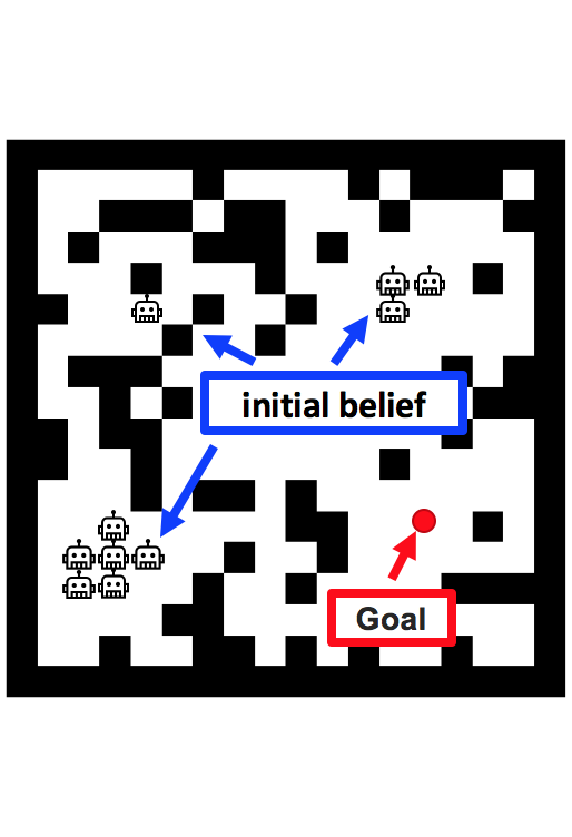
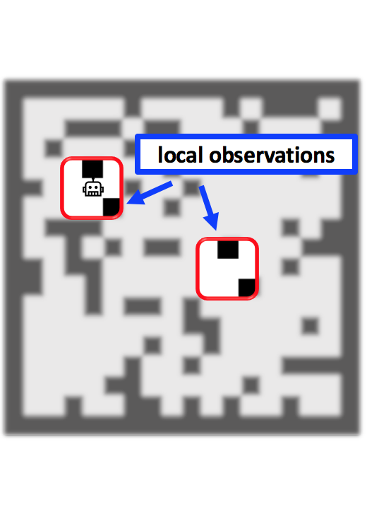
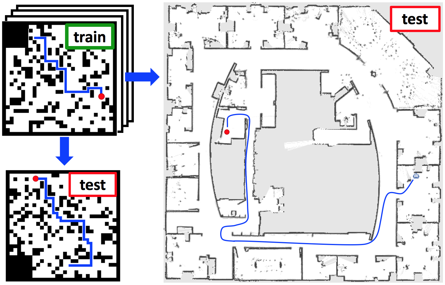
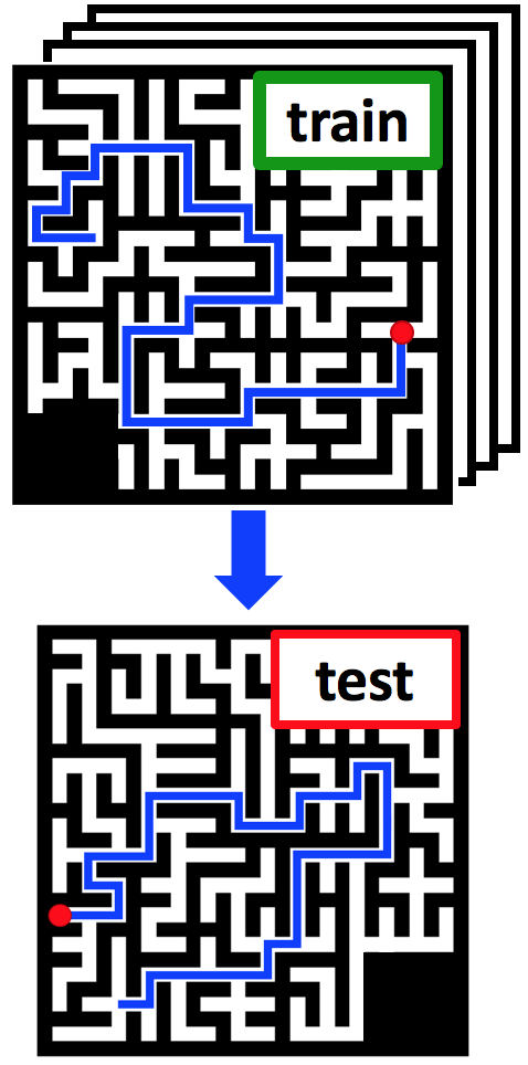
Fig. 1: A robot learning to navigate in partially observable grid worlds. (a) The robot has a map. It has a belief over the initial state, but does not know the exact initial state. (b) Local observations are ambiguous and are insufficient to determine the exact state. (c, d) A policy trained on expert demonstrations in a set of randomly generated environments generalizes to a new environment. It also “transfers” to a much larger real-life environment, represented as a LIDAR map [12].

We train a QMDP-net on expert demonstrations in a set of randomly generated environments. The trained policy generalizes to new environments and also “transfers” to more complex environments (Fig. 1c–d). Preliminary experiments show that QMDP-net outperformed state-of-the-art network architectures on several robotic tasks in simulation. It successfully solved difficult POMDPs that require reasoning over many time steps, such as the well-known Hallway2 domain [18]. Interestingly, while QMDP-net encodes the QMDP algorithm, it sometimes outperformed the QMDP algorithm in our experiments, as a result of end-to-end learning.

2 Background

2.1 Planning under Uncertainty

A POMDP is formally defined as a tuple $(S,A,O,T,Z,R)$, where $S$, $A$ and $O$ are the state, action, and observation space, respectively. The state-transition function $T(s,a,s^{\prime})=P(s^{\prime}|s,a)$ defines the probability of the agent being in state $s^{\prime}$ after taking action $a$ in state $s$. The observation function $Z(s,a,o)=p(o|s,a)$ defines the probability of receiving observation $o$ after taking action $a$ in state $s$. The reward function $R(s,a)$ defines the immediate reward for taking action $a$ in state $s$.

In a partially observable world, the agent does not know its exact state. It maintains a belief, which is a probability distribution over $S$. The agent starts with an initial belief $b_{0}$ and updates the belief $b_{t}$ at each time step $t$ with a Bayesian filter:

$$\textstyle b_{t}(s^{\prime})=\tau(b_{t-1},a_{t},o_{t})=\eta O(s^{\prime},a_{t},o_{t})\sum_{s\in S}T(s,a_{t},s^{\prime})b_{t-1}(s),\vspace*{-2pt}$$ (1)

where $\eta$ is a normalizing constant. The belief $b_{t}$ recursively integrates information from the entire past history $(a_{1},o_{1},a_{2},o_{2},\ldots,a_{t},o_{t})$ for decision making. POMDP planning seeks a policy $\pi$ that maximizes the value, i.e., the expected total discounted reward:

$$\textstyle V_{\pi}(b_{0})=\mathbb{E}\bigl{(}\sum_{t=0}^{\infty}\gamma^{t}R(s_{t},a_{t+1})\;\bigl{|}\;b_{0},\pi\bigr{)},\vspace*{-2pt}$$ (2)

where $s_{t}$ is the state at time $t$, $a_{t+1}=\pi(b_{t})$ is the action that the policy $\pi$ chooses at time $t$, and $\gamma\in(0,1)$ is a discount factor.

2.2 Related Work

To learn policies for decision making in partially observable domains, one approach is to learn models [19, 26, 6] and solve the models through planning. An alternative is to learn policies directly [5, 2]. Model learning is usually not end-to-end. While policy learning can be end-to-end, it does not exploit model information for effective generalization. Our proposed approach combines model-based and model-free learning by embedding a model and a planning algorithm in a recurrent neural network (RNN) that represents a policy and then training the network end-to-end.

RNNs have been used earlier for learning in partially observable domains [11, 4, 10]. In particular, Hausknecht and Stone extended DQN [21], a convolutional neural network (CNN), by replacing its post-convolutional fully connected layer with a recurrent LSTM layer [10]. Similarly, Mirowski et al. [20] considered learning to navigate in partially observable 3-D mazes. The learned policy generalizes over different goals, but in a fixed environment. Instead of using the generic LSTM, our approach embeds algorithmic structure specific to sequential decision making in the network architecture and aims to learn a policy that generalizes to new environments.

The idea of embedding specific computation structures in the neural network architecture has been gaining attention recently. Tamar et al. implemented value iteration in a neural network, called Value Iteration Network (VIN), to solve Markov decision processes (MDPs) in fully observable domains, where an agent knows its exact state and does not require filtering [34]. Okada et al. addressed a related problem of path integral optimal control, which allows for continuous states and actions [23]. Neither addresses the issue of partial observability, which drastically increases the computational complexity of decision making [24]. Haarnoja et al. [9] and Jonschkowski and Brock [15] developed end-to-end trainable Bayesian filters for probabilistic state estimation. Silver et al. introduced Predictron for value estimation in Markov reward processes [31]. They do not deal with decision making or planning. Both Shankar et al. [28] and Gupta et al. [8] addressed planning under partial observability. The former focuses on learning a model rather than a policy. The learned model is trained on a fixed environment and does not generalize to new ones. The latter proposes a network learning approach to robot navigation in an unknown environment, with a focus on mapping. Its network architecture contains a hierarchical extension of VIN for planning and thus does not deal with partial observability during planning. The QMDP-net extends the prior work on network architectures for MDP planning and for Bayesian filtering. It imposes the POMDP model and computation structure priors on the entire network architecture for planning under partial observability.

3 Overview

We want to learn a policy that enables an agent to act effectively in a diverse set of partially observable stochastic environments. Consider, for example, the robot navigation domain in Fig. 1. The environments may correspond to different buildings. The robot agent does not observe its own location directly, but estimates it based on noisy readings from a laser range finder. It has access to building maps, but does not have models of its own dynamics and sensors. While the buildings may differ significantly in their layouts, the underlying reasoning required for effective navigation is similar in all buildings. After training the robot in a few buildings, we want to place the robot in a new building and have it navigate effectively to a specified goal.

Formally, the agent learns a policy for a parameterized set of tasks in partially observable stochastic environments: $\mathcal{W}_{\Theta}=\{W(\boldsymbol{\theta})\mid\boldsymbol{\theta}\in\Theta\}$, where $\Theta$ is the set of all parameter values. The parameter value $\boldsymbol{\theta}$ captures a wide variety of task characteristics that vary within the set, including environments, goals, and agents. In our robot navigation example, $\boldsymbol{\theta}$ encodes a map of the environment, a goal, and a belief over the robot’s initial state. We assume that all tasks in $\mathcal{W}_{\Theta}$ share the same state space, action space, and observation space. The agent does not have prior models of its own dynamics, sensors, or task objectives. After training on tasks for some subset of values in $\Theta$, the agent learns a policy that solves $W(\boldsymbol{\theta})$ for any given $\boldsymbol{\theta}\in\Theta$.

A key issue is a general representation of a policy for $\mathcal{W}_{\Theta}$, without knowing the specifics of $\mathcal{W}_{\Theta}$ or its parametrization. We introduce the QMDP-net, a recurrent policy network. A QMDP-net represents a policy by connecting a parameterized POMDP model with an approximate POMDP algorithm and embedding both in a single, differentiable neural network. Embedding the model allows the policy to generalize over $\mathcal{W}_{\Theta}$ effectively. Embedding the algorithm allows us to train the entire network end-to-end and learn a model that compensates for the limitations of the approximate algorithm.

Let $M(\boldsymbol{\theta})=(S,A,O,f_{\scriptscriptstyle T}(\cdot|\boldsymbol{\theta}),f_{\scriptscriptstyle Z}(\cdot|\boldsymbol{\theta}),f_{\scriptscriptstyle R}(\cdot|\boldsymbol{\theta}))$ be the embedded POMDP model, where $S,A$ and $O$ are the shared state space, action space, observation space designed manually for all tasks in $\mathcal{W}_{\Theta}$ and $f_{\scriptscriptstyle T}(\cdot|\cdot),f_{\scriptscriptstyle Z}(\cdot|\cdot),f_{\scriptscriptstyle R}(\cdot|\cdot)$ are the state-transition, observation, and reward functions to be learned from data. It may appear that a perfect answer to our learning problem would have $f_{\scriptscriptstyle T}(\cdot|\boldsymbol{\theta}),f_{\scriptscriptstyle Z}(\cdot|\boldsymbol{\theta}),\text{ and }f_{\scriptscriptstyle R}(\cdot|\boldsymbol{\theta})$ represent the “true” underlying models of dynamics, observation, and reward for the task $W(\boldsymbol{\theta})$. This is true only if the embedded POMDP algorithm is exact, but not true in general. The agent may learn an alternative model to mitigate an approximate algorithm’s limitations and obtain an overall better policy. In this sense, while QMDP-net embeds a POMDP model in the network architecture, it aims to learn a good policy rather than a “correct” model.

A QMDP-net consists of two modules (Fig. 2). One encodes a Bayesian filter, which performs state estimation by integrating the past history of agent actions and observations into a belief. The other encodes QMDP, a simple, but fast approximate POMDP planner [18]. QMDP chooses the agent’s actions by solving the corresponding fully observable Markov decision process (MDP) and performing one-step look-ahead search on the MDP values weighted by the belief.

[figure]style=plain,subcapbesideposition=top

[][]     [][]     [][]

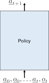
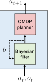
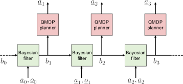
Fig. 2: QMDP-net architecture. LABEL:sub@fig:rnn1 A policy maps a history of actions and observations to a new action. LABEL:sub@fig:rnn2 A QMDP-net is an RNN that imposes structure priors for sequential decision making under partial observability. It embeds a Bayesian filter and the QMDP algorithm in the network. The hidden state of the RNN encodes the belief for POMDP planning. LABEL:sub@fig:rnn3 A QMDP-net unfolded in time.

We evaluate the proposed network architecture in an imitation learning setting. We train on a set of expert trajectories with randomly chosen task parameter values in $\Theta$ and test with new parameter values. An expert trajectory consist of a sequence of demonstrated actions and observations $(a_{1},o_{1},a_{2},o_{2},\ldots)$ for some $\boldsymbol{\theta}\in\Theta$. The agent does not access the ground-truth states or beliefs along the trajectory during the training. We define loss as the cross entropy between predicted and demonstrated action sequences and use RMSProp [35] for training. See Appendix C.7 for details. Our implementation in Tensorflow [1] is available online at http://github.com/AdaCompNUS/qmdp-net.

4 QMDP-Net

We assume that all tasks in a parameterized set $\mathcal{W}_{\Theta}$ share the same underlying state space $\underline{S}$, action space $\underline{A}$, and observation space $\underline{O}$. We want to learn a QMDP-net policy for $\mathcal{W}_{\Theta}$, conditioned on the parameters $\boldsymbol{\theta}\in\Theta$. A QMDP-net is a recurrent policy network. The inputs to a QMDP-net are the action $\underline{a}_{t}\in\underline{A}$ and the observation $\underline{o}_{t}\in\underline{O}$ at time step $t$, as well as the task parameter $\boldsymbol{\theta}\in\Theta$. The output is the action $\underline{a}_{t+1}$ for time step $t+1$.

A QMDP-net encodes a parameterized POMDP model $M(\boldsymbol{\theta})=(S,A,O,T=f_{\scriptscriptstyle T}(\cdot|\boldsymbol{\theta}),Z=f_{\scriptscriptstyle Z}(\cdot|\boldsymbol{\theta}),R=f_{\scriptscriptstyle R}(\cdot|\boldsymbol{\theta}))$ and the QMDP algorithm, which selects actions by solving the model approximately. We choose $S$, $A$, and $O$ of $M(\boldsymbol{\theta})$ manually, based on prior knowledge on $\mathcal{W}_{\Theta}$, specifically, prior knowledge on $\underline{S}$, $\underline{A}$, and $\underline{O}$. In general, $S\not=\underline{S}$, $A\not=\underline{A}$, and $O\not=\underline{O}$. The model states, actions, and observations may be abstractions of their real-world counterparts in the task. In our robot navigation example (Fig. 1), while the robot moves in a continuous space, we choose $S$ to be a grid of finite size. We can do the same for $A$ and $O$, in order to reduce representational and computational complexity. The transition function $T$, observation function $Z$, and reward function $R$ of $M(\boldsymbol{\theta})$ are conditioned on $\boldsymbol{\theta}$, and are learned from data through end-to-end training. In this work, we assume that $T$ is the same for all tasks in $\mathcal{W}_{\Theta}$ to simplify the network architecture. In other words, $T$ does not depend on $\boldsymbol{\theta}$.

End-to-end training is feasible, because a QMDP-net encodes both a model and the associated algorithm in a single, fully differentiable neural network. The main idea for embedding the algorithm in a neural network is to represent linear operations, such as matrix multiplication and summation, by convolutional layers and represent maximum operations by max-pooling layers. Below we provide some details on the QMDP-net’s architecture, which consists of two modules, a filter and a planner.

[figure]style=plain, capposition=bottom

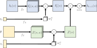
(a)

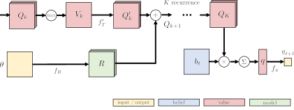
(b)

Fig. 3: A QMDP-net consists of two modules. LABEL:sub@fig:filter The Bayesian filter module incorporates the current action $\underline{a}_{t}$ and observation $\underline{o}_{t}$ into the belief. LABEL:sub@fig:planner The QMDP planner module selects the action according to the current belief $b_{t}$.

Filter module.

The filter module (Fig. 3a) implements a Bayesian filter. It maps from a belief, action, and observation to a next belief, $b_{t+1}=f(b_{t}|\underline{a}_{t},\underline{o}_{t})$. The belief is updated in two steps. The first accounts for actions, the second for observations:

$$\textstyle b^{\prime}_{t}(s)=\sum_{s^{\prime}\in S}{T(s,\underline{a}_{t},s^{\prime})b_{t}(s^{\prime})},$$ (3)

$$\textstyle b_{t+1}(s)=\eta Z(s,\underline{o}_{t})b^{\prime}_{t}(s),$$ (4)

where $\underline{o}_{t}\in\underline{O}$ is the observation received after taking action $\underline{a}_{t}\in\underline{A}$ and $\eta$ is a normalization factor.

We implement the Bayesian filter by transforming Eq. (3) and Eq. (4) to layers of a neural network. For ease of discussion consider our $N\times N$ grid navigation task (Fig. 1a–c). The agent does not know its own state and only observes neighboring cells. It has access to the task parameter $\boldsymbol{\theta}$ that encodes the obstacles, goal, and a belief over initial states. Given the task, we choose $M(\boldsymbol{\theta})$ to have a $N\times N$ state space. The belief, $b_{t}(s)$, is now an $N\times N$ tensor.

Eq. (3) is implemented as a convolutional layer with $|A|$ convolutional filters. We denote the convolutional layer by $f_{\scriptscriptstyle T}$. The kernel weights of $f_{\scriptscriptstyle T}$ encode the transition function $T$ in $M(\boldsymbol{\theta})$. The output of the convolutional layer, $b_{t}^{\prime}(s,a)$, is a $N\times N\times|A|$ tensor.

$b_{t}^{\prime}(s,a)$ encodes the updated belief after taking each of the actions, $a\in A$. We need to select the belief corresponding to the last action taken by the agent, $\underline{a}_{t}$. We can directly index $b_{t}^{\prime}(s,a)$ by $\underline{a}_{t}$ if $A=\underline{A}$. In general $A\not=\underline{A}$, so we cannot use simple indexing. Instead, we will use “soft indexing”. First we encode actions in $\underline{A}$ to actions in $A$ through a learned function $f_{\scriptscriptstyle A}$. $f_{\scriptscriptstyle A}$ maps from $\underline{a}_{t}$ to an indexing vector $w^{a}_{t}$, a distribution over actions in $A$. We then weight $b^{\prime}_{t}(s,a)$ by $w^{a}_{t}$ along the appropriate dimension, i.e.

$$\textstyle{b^{\prime}_{t}}(s)=\sum_{a\in A}{b^{\prime}_{t}(s,a)w^{a}_{t}}.$$ (5)

Eq. (4) incorporates observations through an observation model $Z(s,o)$. Now $Z(s,o)$ is a $N\times N\times|O|$ tensor that represents the probability of receiving observation $o\in O$ in state $s\in S$. In our grid navigation task observations depend on the obstacle locations. We condition $Z$ on the task parameter, $Z(s,o)=f_{\scriptscriptstyle Z}(s,o|\boldsymbol{\theta})$ for $\boldsymbol{\theta}\in\Theta$. The function $f_{\scriptscriptstyle Z}$ is a neural network, mapping from $\boldsymbol{\theta}$ to $Z(s,o)$. In this paper $f_{\scriptscriptstyle Z}$ is a CNN.

$Z(s,o)$ encodes observation probabilities for each of the observations, $o\in O$. We need the observation probabilities for the last observation $\underline{o}_{t}$. In general $O\not=\underline{O}$ and we cannot index $Z(s,o)$ directly. Instead, we will use soft indexing again. We encode observations in $\underline{O}$ to observations in $O$ through $f_{\scriptscriptstyle O}$. $f_{\scriptscriptstyle O}$ is a function mapping from $\underline{o}_{t}$ to an indexing vector, $w^{o}_{t}$, a distribution over $O$. We then weight $Z(s,o)$ by $w^{o}_{t}$, i.e.

$$\textstyle Z(s)=\sum_{o\in O}Z(s,o)w^{o}_{t}.$$ (6)

Finally, we obtain the updated belief, $b_{t+1}(s)$, by multiplying ${b^{\prime}_{t}}(s)$ and $Z(s)$ element-wise, and normalizing over states. In our setting the initial belief for the task $W(\boldsymbol{\theta})$ is encoded in $\boldsymbol{\theta}$. We initialize the belief in QMDP-net through an additional encoding function, $b_{0}=f_{\scriptscriptstyle B}(\boldsymbol{\theta})$.

Planner module.

The QMDP planner (Fig. 3b) performs value iteration at its core. $Q$ values are computed by iteratively applying Bellman updates,

$$\textstyle Q_{k+1}(s,a)=R(s,a)+\gamma\sum_{s^{\prime}\in S}{T(s,a,s^{\prime})V_{k}(s^{\prime})},$$ (7)

$$\textstyle V_{k}(s)=\max_{a}{Q_{k}(s,a)}.$$ (8)

Actions are then selected by weighting the $Q$ values with the belief.

We can implement value iteration using convolutional and max pooling layers [34, 28]. In our grid navigation task $Q(s,a)$ is a $N\times N\times|A|$ tensor. Eq. (8) is expressed by a max pooling layer, where $Q_{k}(s,a)$ is the input and $V_{k}(s)$ is the output. Eq. (7) is a $N\times N$ convolution with $|A|$ convolutional filters, followed by an addition operation with $R(s,a)$, the reward tensor. We denote the convolutional layer by $f_{\scriptscriptstyle T}^{\prime}$. The kernel weights of $f_{\scriptscriptstyle T}^{\prime}$ encode the transition function $T$, similarly to $f_{\scriptscriptstyle T}$ in the filter. Rewards for a navigation task depend on the goal and obstacles. We condition rewards on the task parameter, $R(s,a)=f_{\scriptscriptstyle R}(s,a|\boldsymbol{\theta})$. $f_{\scriptscriptstyle R}$ maps from $\boldsymbol{\theta}$ to $R(s,a)$. In this paper $f_{\scriptscriptstyle R}$ is a CNN.

We implement $K$ iterations of Bellman updates by stacking the layers representing Eq. (7) and Eq. (8) $K$ times with tied weights. After $K$ iterations we get $Q_{K}(s,a)$, the approximate $Q$ values for each state-action pair. We weight the $Q$ values by the belief to obtain action values,

$$\textstyle q(a)=\sum_{s\in S}{Q_{K}(s,a)b_{t}(s)}.$$ (9)

Finally, we choose the output action through a low-level policy function, $f_{\scriptscriptstyle\pi}$, mapping from $q(a)$ to the action output, $\underline{a}_{t+1}$.

QMDP-net naturally extends to higher dimensional discrete state spaces (e.g. our maze navigation task) where $n$-dimensional convolutions can be used [14]. While $M(\boldsymbol{\theta})$ is restricted to a discrete space, we can handle continuous tasks $\mathcal{W}_{\Theta}$ by simultaneously learning a discrete $M(\boldsymbol{\theta})$ for planning, and $f_{\scriptscriptstyle A},f_{\scriptscriptstyle O},f_{\scriptscriptstyle B},f_{\scriptscriptstyle\pi}$ to map between states, actions and observations in $\mathcal{W}_{\Theta}$ and $M(\boldsymbol{\theta})$.

5 Experiments

The main objective of the experiments is to understand the benefits of structure priors on learning neural-network policies. We create several alternative network architectures by gradually relaxing the structure priors and evaluate the architectures on simulated robot navigation and manipulation tasks. While these tasks are simpler than, for example, Atari games, in terms of visual perception, they are in fact very challenging, because of the sophisticated long-term reasoning required to handle partial observability and distant future rewards. Since the exact state of the robot is unknown, a successful policy must reason over many steps to gather information and improve state estimation through partial and noisy observations. It also must reason about the trade-off between the cost of information gathering and the reward in the distance future.

5.1 Experimental Setup

We compare the QMDP-net with a number of related alternative architectures. Two are QMDP-net variants. Untied QMDP-net relaxes the constraints on the planning module by untying the weights representing the state-transition function over the different CNN layers. LSTM QMDP-net replaces the filter module with a generic LSTM module. The other two architectures do not embed POMDP structure priors at all. CNN+LSTM is a state-of-the-art deep CNN connected to an LSTM. It is similar to the DRQN architecture proposed for reinforcement learning under partially observability [10]. RNN is a basic recurrent neural network with a single fully-connected hidden layer. RNN contains no structure specific to planning under partial observability.

Each experimental domain contains a parameterized set of tasks $\mathcal{W}_{\Theta}$. The parameters $\boldsymbol{\theta}$ encode an environment, a goal, and a belief over the robot’s initial state. To train a policy for $\mathcal{W}_{\Theta}$, we generate random environments, goals, and initial beliefs. We construct ground-truth POMDP models for the generated data and apply the QMDP algorithm. If the QMDP algorithm successfully reaches the goal, we then retain the resulting sequence of action and observations $(a_{1},o_{1},a_{2},o_{2},\ldots)$ as an expert trajectory, together with the corresponding environment, goal, and initial belief. It is important to note that the ground-truth POMDPs are used only for generating expert trajectories and not for learning the QMDP-net.

For fair comparison, we train all networks using the same set of expert trajectories in each domain. We perform basic search over training parameters, the number of layers, and the number of hidden units for each network architecture. Below we briefly describe the experimental domains. See Appendix C for implementation details.

Grid-world navigation.

A robot navigates in an unknown building given a floor map and a goal. The robot is uncertain of its own location. It is equipped with a LIDAR that detects obstacles in its direct neighborhood. The world is uncertain: the robot may fail to execute desired actions, possibly because of wheel slippage, and the LIDAR may produce false readings. We implemented a simplified version of this task in a discrete $n\times n$ grid world (Fig. 1c). The task parameter $\boldsymbol{\theta}$ is represented as an $n\times n$ image with three channels. The first channel encodes the obstacles in the environment, the second channel encodes the goal, and the last channel encodes the belief over the robot’s initial state. The robot’s state represents its position in the grid. It has five actions: moving in each of the four canonical directions or staying put. The LIDAR observations are compressed into four binary values corresponding to obstacles in the four neighboring cells. We consider both a deterministic and a stochastic variant of the domain. The stochastic variant adds action and observation uncertainties. The robot fails to execute the specified move action and stays in place with probability $0.2$. The observations are faulty with probability $0.1$ independently in each direction. We trained a policy using expert trajectories from $10,000$ random environments, $5$ trajectories from each environment. We then tested on a separate set of $500$ random environments.

Maze navigation.

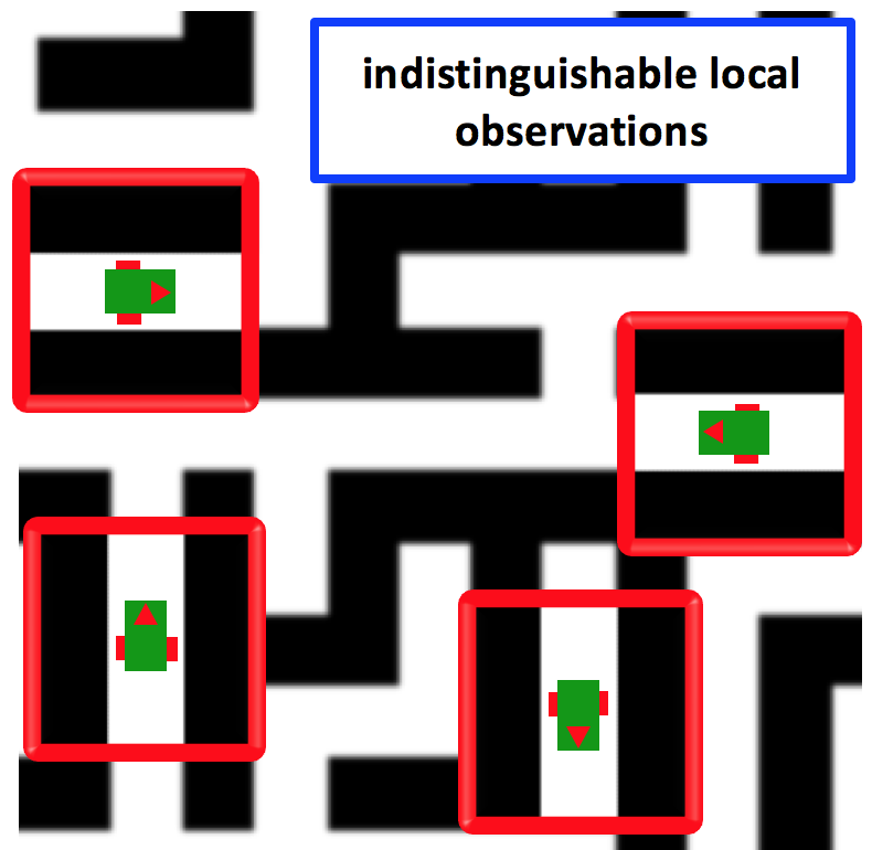
Fig. 4: Highly ambiguous observations in a maze. The four observations (in red) are the same, despite that the robot states are all different.

A differential-drive robot navigates in a maze with the help of a map, but it does not know its pose (Fig. 1). This domain is similar to the grid-world navigation, but it is significant more challenging. The robot’s state contains both its position and orientation. The robot cannot move freely because of kinematic constraints. It has four actions: move forward, turn left, turn right and stay put. The observations are relative to the robot’s current orientation, and the increased ambiguity makes it more difficult to localize the robot, especially when the initial state is highly uncertain. Finally, successful trajectories in mazes are typically much longer than those in randomly-generated grid worlds. Again we trained on expert trajectories in $10,000$ randomly generated mazes and tested them in $500$ new ones.

2-D object grasping.

[figure]style=plain,subcapbesideposition=top

[][]   [][]

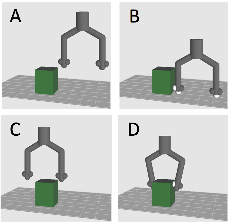
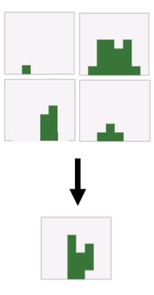
Fig. 5: Object grasping using touch sensing. LABEL:sub@fig:grasp_a An example [3]. LABEL:sub@fig:grasp_b Simplified 2-D object grasping. Objects from the training set (top) and the test set (bottom).

A robot gripper picks up novel objects from a table using a two-finger hand with noisy touch sensors at the finger tips. The gripper uses the fingers to perform compliant motions while maintaining contact with the object or to grasp the object. It knows the shape of the object to be grasped, maybe from an object database. However, it does not know its own pose relative to the object and relies on the touch sensors to localize itself. We implemented a simplified 2-D variant of this task, modeled as a POMDP [13]. The task parameter $\boldsymbol{\theta}$ is an image with three channels encoding the object shape, the grasp point, and a belief over the gripper’s initial pose. The gripper has four actions, each moving in a canonical direction unless it touches the object or the environment boundary. Each finger has $3$ binary touch sensors at the tip, resulting in $64$ distinct observations. We trained on expert demonstration on $20$ different objects with $500$ randomly sampled poses for each object. We then tested on $10$ previously unseen objects in random poses.

5.2 Choosing QMDP-Net Components for a Task

Given a new task $\mathcal{W}_{\Theta}$, we need to choose an appropriate neural network representation for $M(\boldsymbol{\theta})$. More specifically, we need to choose $S,A$ and $O$, and a representation for the functions $f_{\scriptscriptstyle R},f_{\scriptscriptstyle T},f_{\scriptscriptstyle T}^{\prime},f_{\scriptscriptstyle Z},f_{\scriptscriptstyle O},f_{\scriptscriptstyle A},f_{\scriptscriptstyle B},f_{\scriptscriptstyle\pi}$. This provides an opportunity to incorporate domain knowledge in a principled way. For example, if $\mathcal{W}_{\Theta}$ has a local and spatially invariant connectivity structure, we can choose convolutions with small kernels to represent $f_{\scriptscriptstyle T}$, $f_{\scriptscriptstyle R}$ and $f_{\scriptscriptstyle Z}$.

In our experiments we use $S=N\times N$ for $N\times N$ grid navigation, and $S=N\times N\times 4$ for $N\times N$ maze navigation where the robot has $4$ possible orientations. We use $|A|=|\underline{A}|$ and $|O|=|\underline{O}|$ for all tasks except for the object grasping task, where $|\underline{O}|=64$ and $|O|=16$. We represent $f_{\scriptscriptstyle T},f_{\scriptscriptstyle R}$ and $f_{\scriptscriptstyle Z}$ by CNN components with $3\times 3$ and $5\times 5$ kernels depending on the task. We enforce that $f_{\scriptscriptstyle T}$ and $f_{\scriptscriptstyle Z}$ are proper probability distributions by using softmax and sigmoid activations on the convolutional kernels, respectively. Finally, $f_{\scriptscriptstyle O}$ is a small fully connected component, $f_{\scriptscriptstyle A}$ is a one-hot encoding function, $f_{\scriptscriptstyle\pi}$ is a single softmax layer, and $f_{\scriptscriptstyle B}$ is the identity function.

We can adjust the amount of planning in a QMDP-net by setting $K$. A large $K$ allows propagating information to more distant states without affecting the number of parameters to learn. However, it results in deeper networks that are computationally expensive to evaluate and more difficult to train. We used $K=20\dots 116$ depending on the problem size. We were able to transfer policies to larger environments by increasing $K$ up to $450$ when executing the policy.

In our experiments the representation of the task parameter $\boldsymbol{\theta}$ is isomorphic to the chosen state space $S$. While the architecture is not restricted to this setting, we rely on it to represent $f_{\scriptscriptstyle T},f_{\scriptscriptstyle Z},f_{\scriptscriptstyle R}$ by convolutions with small kernels. Experiments with a more general class of problems is an interesting direction for future work.

5.3 Results and Discussion

The main results are reported in Table 1. Some additional results are reported in Appendix A. For each domain, we report the task success rate and the average number of time steps for task completion. Comparing the completion time is meaningful only when the success rates are similar.

QMDP-net successfully learns policies that generalize to new environments.

When evaluated on new environments, the QMDP-net has higher success rate and faster completion time than the alternatives in nearly all domains. To understand better the performance difference, we specifically compared the architectures in a fixed environment for navigation. Here only the initial state and the goal vary across the task instances, while the environment remains the same. See the results in the last row of Table 1. The QMDP-net and the alternatives have comparable performance. Even RNN performs very well. Why? In a fixed environment, a network may learn the features of an optimal policy directly, e.g., going straight towards the goal. In contrast, the QMDP-net learns a model for planning, i.e., generating a near-optimal policy for a given arbitrary environment.

POMDP structure priors improve the performance of learning complex policies.

Moving across Table 1 from left to right, we gradually relax the POMDP structure priors on the network architecture. As the structure priors weaken, so does the overall performance. However, strong priors sometimes over-constrain the network and result in degraded performance. For example, we found that tying the weights of $f_{\scriptscriptstyle T}$ in the filter and $f_{\scriptscriptstyle T}^{\prime}$ in the planner may lead to worse policies. While both $f_{\scriptscriptstyle T}$ and $f_{\scriptscriptstyle T}^{\prime}$ represent the same underlying transition dynamics, using different weights allows each to choose its own approximation and thus greater flexibility. We shed some light on this issue and visualize the learned POMDP model in Appendix B.

[table]capposition=top

Table 1: Performance comparison of QMDP-net and alternative architectures for recurrent policy networks. SR is the success rate in percentage. Time is the average number of time steps for task completion. D-$n$ and S-$n$ denote deterministic and stochastic variants of a domain with environment size $n\times n$.

	QMDP		QMDP-net		Untied		LSTM		CNN		RNN
					QMDP-net		QMDP-net		+LSTM
Domain	SR	Time	SR	Time	SR	Time	SR	Time	SR	Time	SR	Time
Grid D-10	$99.8$	$8.8$	$99.6$	$8.2$	$98.6$	$8.3$	$84.4$	$12.8$	$90.0$	$13.4$	$87.8$	$13.4$
Grid D-18	$99.0$	$15.5$	$99.0$	$14.6$	$98.8$	$14.8$	$43.8$	$27.9$	$57.8$	$33.7$	$35.8$	$24.5$
Grid D-30	$97.6$	$24.6$	$98.6$	$25.0$	$98.8$	$23.9$	$22.2$	$51.1$	$19.4$	$45.2$	$16.4$	$39.3$
Grid S-18	$98.1$	$23.9$	$98.8$	$23.9$	$95.9$	$24.0$	$23.8$	$55.6$	$41.4$	$65.9$	$34.0$	$64.1$
Maze D-29	$63.2$	$54.1$	$98.0$	$56.5$	$95.4$	$62.5$	$9.8$	$57.2$	$9.2$	$41.4$	$9.8$	$47.0$
Maze S-19	$63.1$	$50.5$	$93.9$	$60.4$	$98.7$	$57.1$	$18.9$	$79.0$	$19.2$	$80.8$	$19.6$	$82.1$
Hallway2	$37.3$	$28.2$	$82.9$	$64.4$	$69.6$	$104.4$	$82.8$	$89.7$	$77.8$	$99.5$	$68.0$	$108.8$
Grasp	$98.3$	$14.6$	$99.6$	$18.2$	$98.9$	$20.4$	$91.4$	$26.4$	$92.8$	$22.1$	$94.1$	$25.7$
Intel Lab	$90.2$	$85.4$	$94.4$	$107.7$	$20.0$	$55.3$	-		-		-
Freiburg	$88.4$	$66.9$	$93.2$	$81.1$	$37.4$	$51.7$	-		-		-
Fixed grid	$98.8$	$17.4$	$98.6$	$17.6$	$99.8$	$17.0$	$97.0$	$19.7$	$98.4$	$19.9$	$98.0$	$19.8$

QMDP-net learns “incorrect”, but useful models.

Planning under partial observability is intractable in general, and we must rely on approximation algorithms. A QMDP-net encodes both a POMDP model and QMDP, an approximate POMDP algorithm that solves the model. We then train the network end-to-end. This provides the opportunity to learn an “incorrect”, but useful model that compensates the limitation of the approximation algorithm, in a way similar to reward shaping in reinforcement learning [22]. Indeed, our results show that the QMDP-net achieves higher success rate than QMDP in nearly all tasks. In particular, QMDP-net performs well on the well-known Hallway2 domain, which is designed to expose the weakness of QMDP resulting from its myopic planning horizon. The planning algorithm is the same for both the QMDP-net and QMDP, but the QMDP-net learns a more effective model from expert demonstrations. This is true even though QMDP generates the expert data for training. We note that the expert data contain only successful QMDP demonstrations. When both successful and unsuccessful QMDP demonstrations were used for training, the QMDP-net did not perform better than QMDP, as one would expect.

QMDP-net policies learned in small environments transfer directly to larger environments.

Learning a policy for large environments from scratch is often difficult. A more scalable approach would be to learn a policy in small environments and transfer it to large environments by repeating the reasoning process. To transfer a learned QMDP-net policy, we simply expand its planning module by adding more recurrent layers. Specifically, we trained a policy in randomly generated $30\times 30$ grid worlds with $K=90$. We then set $K=450$ and applied the learned policy to several real-life environments, including Intel Lab ($100\times 101$) and Freiburg ($139\times 57$), using their LIDAR maps (Fig. 1c) from the Robotics Data Set Repository [12]. See the results for these two environments in Table 1. Additional results with different $K$ settings and other buildings are available in Appendix A.

6 Conclusion

A QMDP-net is a deep recurrent policy network that embeds POMDP structure priors for planning under partial observability. While generic neural networks learn a direct mapping from inputs to outputs, QMDP-net learns how to model and solve a planning task. The network is fully differentiable and allows for end-to-end training.

Experiments on several simulated robotic tasks show that learned QMDP-net policies successfully generalize to new environments and transfer to larger environments as well. The POMDP structure priors and end-to-end training substantially improve the performance of learned policies. Interestingly, while a QMDP-net encodes the QMDP algorithm for planning, learned QMDP-net policies sometimes outperform QMDP.

There are many exciting directions for future exploration. First, a major limitation of our current approach is the state space representation. The value iteration algorithm used in QMDP iterates through the entire state space and is well known to suffer from the “curse of dimensionality”. To alleviate this difficulty, the QMDP-net, through end-to-end training, may learn a much smaller abstract state space representation for planning. One may also incorporate hierarchical planning [8]. Second, QMDP makes strong approximations in order to reduce computational complexity. We want to explore the possibility of embedding more sophisticated POMDP algorithms in the network architecture. While these algorithms provide stronger planning performance, their algorithmic sophistication increases the difficulty of learning. Finally, we have so far restricted the work to imitation learning. It would be exciting to extend it to reinforcement learning. Based on earlier work [28, 34], this is indeed promising.

Acknowledgments

We thank Leslie Kaelbling and Tomás Lozano-Pérez for insightful discussions that helped to improve our understanding of the problem. The work is supported in part by Singapore Ministry of Education AcRF grant MOE2016-T2-2-068 and National University of Singapore AcRF grant R-252-000-587-112.

Appendix A Supplementary Experiments

A.1 Navigation on Large LIDAR Maps

We provide results on additional environments for the LIDAR map navigation task. LIDAR maps are obtained from [33]. See Section C.5 for details. Intel corresponds to Intel Research Lab. Freiburg corresponds to Freiburg, Building 079. Belgioioso corresponds to Belgioioso Castle. MIT corresponds to the western wing of the MIT CSAIL building. We note the size of the grid size $NxM$ for each environment. A QMDP-net policy is trained on the $30x30$-D grid navigation domain on randomly generated environments using $K=90$. We then execute the learned QMDP-net policy with different $K$ settings, i.e. we add convolutional layers to the planner that share the same kernel weights. We report the task success rate and the average number of time steps for task completion.

[table]capposition=top

Table 2: Additional results for navigation on large LIDAR maps.

	QMDP		QMDP-net		QMDP-net		QMDP-net		Untied
			K=450		K=180		K=90		QMDP-net
Domain	SR	Time	SR	Time	SR	Time	SR	Time	SR	Time
Intel $100\times 101$	$90.2$	$85.4$	94.4	$108.0$	$83.4$	$89.6$	$40.8$	$78.6$	$20.0$	$55.3$
Freiburg $139\times 57$	$88.4$	$66.9$	$92.0$	$91.4$	93.2	$81.1$	$55.8$	$68.0$	$37.4$	$51.7$
Belgioioso $151\times 35$	$95.8$	$63.9$	95.4	$71.8$	$90.6$	$62.0$	$60.0$	$54.3$	$41.0$	$47.7$
MIT $41\times 83$	$94.4$	$42.6$	$91.4$	$53.8$	96.0	$48.5$	$86.2$	$45.4$	$66.6$	$41.4$

In the conventional setting, when value iteration is executed on a fully known MDP, increasing $K$ improves the value function approximation and improves the policy in return for the increased computation. In a QMDP-net increasing $K$ has two effects on the overall planning quality. Estimation accuracy of the latent values increases and reward information can propagate to more distant states. On the other hand the learned latent model does not necessarily fit the true underlying model, and it can be overfitted to the $K$ setting during training. Therefore a too high $K$ can degrade the overall performance. We found that $K_{test}=2K_{train}$ significantly improved success rates in all our test cases. Further increasing $K_{test}=5K_{train}$ was beneficial in the Intel and Belgioioso environments, but it slightly decreased success rates for the Freiburg and MIT environments.

We compare QMDP-net to its untied variant, Untied QMDP-net. We cannot expand the layers of Untied QMDP-net during execution. In consequence, the performance is poor. Note that the other alternative architectures we considered are specific to the input size and thus they are not applicable.

A.2 Learning “Incorrect” but Useful Models

We demonstrate that an “incorrect” model can result in better policies when solved by the approximate QMDP algorithm. We compute QMDP policies on a POMDP with modified reward values, then evaluate the policies using the original rewards. We use the deterministic $29\times 29$ maze navigation task where QMDP did poorly. We attempt to shape rewards manually. Our motivation is to break symmetry in the model, and to implicitly encourage information gathering and compensate for the one-step look-ahead approximation in QMDP. Modified 1. We increase the cost for the stay actions to $20$ times of its original value. Modified 2. We increase the cost for the stay action to $50$ times of its original value, and the cost for the turn right action to $10$ times of its original value.

[table]capposition=top

Table 3: QMDP policies computed on an “incorrect” model and evaluated on the “correct” model.

			Original
Variant	SR	Time	reward
Original	63.2	54.1	1.09
Modified 1	65.0	58.1	1.71
Modified 2	93.0	71.4	4.96

Why does the “correct” model result in poor policies when solved by QMDP? At a given point the $Q$ value for a set of possible states may be high for the turn left action and low for the turn right action; while for another set of states it may be the opposite way around. In expectation, both next states have lower value than the current one, thus the policy chooses the stay action, the robot does not gather information and it is stuck in one place. Results demonstrate that planning on an “incorrect” model may improve the performance on the “correct” model.

Appendix B Visualizing the Learned Model

B.1 Value Function

We plot the value function predicted by a QMDP-net for the $18\times 18$ stochastic grid navigation task. We used $K=54$ iterations in the QMDP-net. As one would expect, states close to the goal have high values.

[figure]style=plain,subcapbesideposition=top

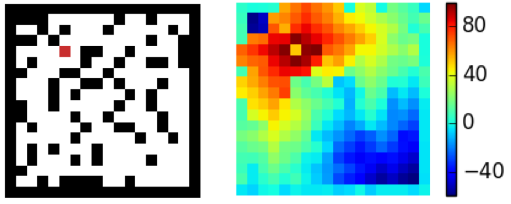
Fig. 6: Map of a test environment and the corresponding learned value function $V_{K}$.

B.2 Belief Propagation

We plot the execution of a learned QMDP-net policy and the internal belief propagation on the $18\times 18$ stochastic grid navigation task. The first row in Fig. 7 shows the environment including the goal (red) and the unobserved pose of the robot (blue). The second row shows ground-truth beliefs for reference. We do not access ground-truth beliefs during training except for the initial belief. The third row shows beliefs predicted by a QMDP-net. The last row shows the difference between the ground-truth and predicted beliefs.

[figure]style=plain,subcapbesideposition=top

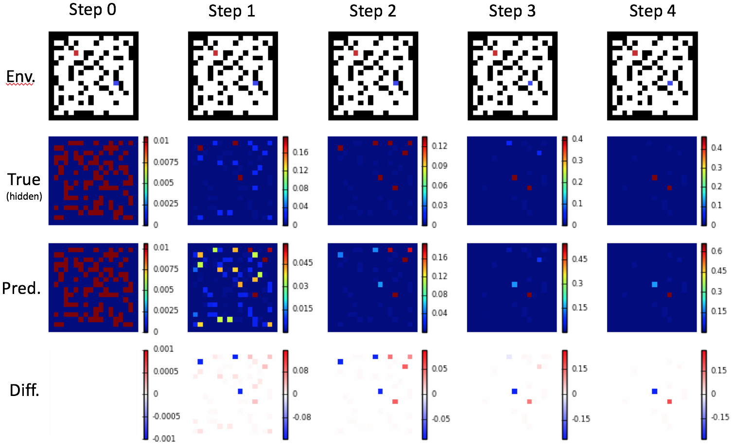
Fig. 7: Policy execution and belief propagation in the $18\times 18$ stochastic grid navigation task.

The figure demonstrates that QMDP-net was able to learn a reasonable filter for state estimation in a noisy environment. In the depicted example the initial belief is uniform over approximately half of the state space (Step 0). Due to the highly uncertain initial belief and the observation noise the robot stays in place for two steps (Step 1 and 2). After two steps the state estimation is still highly uncertain, but it is mostly spread out right from the goal. Therefore, moving left is a reasonable choice (Step 3). After an additional stay action (Step 4) the belief distribution is small enough and the robot starts moving towards the goal (not shown).

B.3 State-Transition Function

We plot the learned and ground-truth state-transition functions. Columns of the table correspond to actions. The first row shows the ground-truth transition function. The second row shows $f_{\scriptscriptstyle T}$, the learned state-transition function in the filter. The third row shows $f_{\scriptscriptstyle T}^{\prime}$, the learned state-transition function in the planner.

[figure]style=plain,subcapbesideposition=top

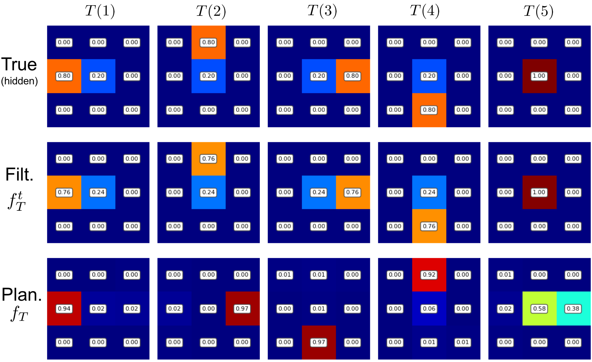
Fig. 8: Learned transition function $T$ in the $18\times 18$ stochastic grid navigation task.

While both $f_{\scriptscriptstyle T}$ and $f_{\scriptscriptstyle T}^{\prime}$ represent the same underlying transition dynamics, the learned transition probabilities are different in the filter and planner. Different weights allows each module to choose its own approximation and thus provides greater flexibility. The actions in the model $a\in A$ are learned abstractions of the agent’s actions $\underline{a}\in\underline{A}$. Indeed, in the planner the learned transition probabilities for action $a_{i}\in A$ do not match the transition probabilities of $\underline{a}_{i}\in\underline{A}$.

B.4 Reward Function

Next plot the learned reward function $R$ for each action $a\in A$.

[figure]style=plain,subcapbesideposition=top

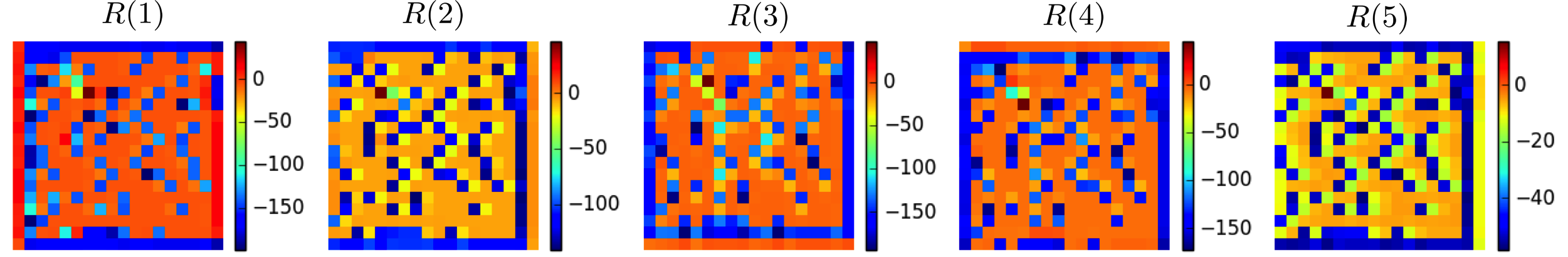
Fig. 9: Learned reward function $R$ in the $18\times 18$ stochastic grid navigation domain.

While the learned rewards do not directly correspond to rewards in the underlying task, they are reasonable: obstacles are assigned negative rewards and the goal is assigned a positive reward. Note that learned reward values correspond to the reward after taking an action, therefore they should be interpreted together with the corresponding transition probabilities (third row of Fig. 8).

Appendix C Implementation Details

C.1 Grid-World Navigation

We implement the grid navigation task in randomly generated discrete $N\times N$ grids where each cell has $p=0.25$ probability of being an obstacle. The robot has $5$ actions: move in the four canonical directions and stay put. Observations are four binary values corresponding to obstacles in the four neighboring cells. We consider a deterministic variant (denoted by -D) and a stochastic variant (denoted by -S). In the stochastic variant the robot fails to execute each action with probability $P_{t}=0.2$, in which case it stays in place. The observations are faulty with probability $P_{o}=0.1$ independently in each direction. Since we receive observations from $4$ directions, the probability of receiving the correct observation vector is only $0.9^{4}=0.656$. The task parameter, $\boldsymbol{\theta}$, is an $N\times N\times 3$ image that encodes information about the environment. The first channel encodes obstacles, $1$ for obstacles, $0$ for free space. The second channel encodes the goal, $1$ for the goal, $0$ otherwise. The third channel encodes the initial belief over robot states, each pixel value corresponds to the probability of the robot being in the corresponding state.

We construct a ground-truth POMDP model to obtain expert trajectories for training. It is important to note that the learning agent has no access to the ground-truth POMDP models. In the ground-truth model the robot receives a reward of $-0.1$ for each step, $+20$ for reaching the goal, and $-10$ for bumping into an obstacle. We use QMDP to solve the POMDP model, and execute the QMDP policy to obtain expert trajectories. We use $10,000$ random grids for training. Initial and goal states are sampled from the free space uniformly. We exclude samples where there is no feasible path. The initial belief is uniform over a random fraction of the free space which includes the underlying initial state. More specifically, the number of non-zero values in the initial-belief are sampled from $\{1,2,\dots N_{f}/2,N_{f}\}$ where $N_{f}$ is the number of free cells in the grid. For each grid we generate $5$ expert trajectories with different initial state, initial belief and goal. Note that we do not access the true beliefs after the first step nor the underlying states along the trajectory.

We test on a set of $500$ environments generated separately in equal conditions. We declare failure after $10N$ steps without reaching the goal. Note that the expert policy is sub-optimal and it may fail to reach the goal. We exclude these samples from the training set but include them in the test set.

We choose the structure of $M(\boldsymbol{\theta})$, the model in QMDP-net, to match the structure of the underlying task. The transition function in the filter $f_{\scriptscriptstyle T}$ and the planner $f_{\scriptscriptstyle T}^{\prime}$ are both $3\times 3$ convolutions. While they both represent the same transition function we do not tie their weights. We apply a softmax function on the kernel matrix so its values sum to one. The reward function, $f_{\scriptscriptstyle R}$, is a CNN with two convolutional layers. The first has $3\times 3$ kernel, $150$ filters, ReLU activation. The second has $1\times 1$ kernel, $5$ filters and linear activation. The observation model, $f_{\scriptscriptstyle Z}$, is a similar two-layer CNN. The first convolution has a $3\times 3$ kernel, $150$ filters, linear activation. The second has $1\times 1$ kernel, $17$ filters and linear activation. The action mapping, $f_{\scriptscriptstyle A}$, is a one-hot encoding function. The observation mapping, $f_{\scriptscriptstyle O}$, is a fully connected network with one hidden layer with $17$ units and tanh activation. It has $17$ output units and softmax activation. The low-level policy function, $f_{\scriptscriptstyle\pi}$, is a single softmax layer. The state space mapping function, $f_{\scriptscriptstyle B}$, is the identity function. Finally, we choose the number of iterations in the planner module, $K=\{30,54,90\}$ for grids of size $N=\{10,18,30\}$ respectively.

The $3\times 3$ convolutions in $f_{\scriptscriptstyle T}$ and $f_{\scriptscriptstyle Z}$ imply that $T$ and $O$ are spatially invariant and local. In the underlying task the locality assumption holds but spatial invariance does not: transitions depend on the arrangement of obstacles. Nevertheless, the additional flexibility in the model allows QMDP-net to learn high-quality policies, e.g. by shaping the rewards and the observation function.

C.2 Maze Navigation

In the maze navigation task a differential drive robot has to navigate to a given goal. We generate random mazes on $N\times N$ grids using Kruskal’s algorithm. The state space has $3$ dimensions where the third dimension represents $4$ possible orientations of the robot. The goal configuration is invariant to the orientation. The robot now has $4$ actions: move forward, turn left, turn right and stay put. The initial belief is chosen in a similar manner to the grid navigation case but in the 3-D space. The observations are identical to grid navigation but they are relative to the robot’s orientation, which significantly increases the difficulty of state estimation. The stochastic variant (denoted by -S) has a motion and observation noise identical to the grid navigation. Training and test data is prepared identically as well. We use $K=\{76,116\}$ for mazes of size $N=\{19,29\}$ respectively.

We use a model in QMDP-net with a $3$-dimensional state space of size $N\times N\times 4$ and an action space with $4$ actions. The components of the network are chosen identically to the previous case, except that all CNN components operate on 3-D tensors of size $N\times N\times 4$. While it would be possible to use 3-D convolutions, we treat the third dimension as channels of a 2-D image instead, and use conventional 2-D convolutions. If the output of the last convolutional layer is of size $N\times N\times N_{c}$ for the grid navigation task, it is of size $N\times N\times 4N_{c}$ for the maze navigation task. When necessary, these tensors are transformed into a $4$ dimensional form $N\times N\times 4\times N_{c}$ and the max-pool or softmax activation is computed along the last dimension.

C.3 Object Grasping

We consider a 2-D implementation of the grasping task based on the POMDP model proposed by Hsiao et al. [13]. Hsiao et al. focused on the difficulty of planning with high uncertainty and solved manually designed POMDPs for single objects. We phrase the problem as a learning task where we have no access to a model and we do not know all objects in advance. In our setting the robot receives an image of the target object and a feasible grasp point, but it does not know its pose relative to the object. We aim to learn a policy on a set of object that generalizes to similar but unseen objects.

The object and the gripper are represented in a discrete grid. The workspace is a $14\times 14$ grid, and the gripper is a “U” shape in the grid. The gripper moves in the four canonical directions, unless it reaches the boundaries of the workspace or it is touching the object. in which case it stays in place. The gripper fails to move with probability $0.2$. The gripper has two fingers with $3$ touch sensors on each finger. The touch sensors indicate contact with the object or reaching the limits of the workspace. The sensors produce an incorrect reading with probability $0.1$ independently for each sensor. In each trial an object is placed on the bottom of the workspace at a random location. The initial gripper pose is unknown; the belief over possible states is uniform over a random fraction of the upper half of the workspace. The local observations, $o_{t}$, are readings from the touch sensors. The task parameter $\boldsymbol{\theta}$ is an image with three channels. The first channel encodes the environment with an object; the second channel encodes the position of the target grasping point; the third channel encodes the initial belief over the gripper position.

We have $30$ artificial objects of different sizes up to $6\times 6$ grid cells. Each object has at least one cell on its top that the gripper can grasp. For training we use $20$ of the objects. We generate $500$ expert trajectories for each object in random configuration. We test the learned policies on $10$ new objects in $20$ random configurations each. The expert trajectories are obtained by solving a ground-truth POMDP model by the QMDP algorithm. In the ground-truth POMDP the robot receives a reward of $1$ for reaching the grasp point and $0$ for every other state.

In QMDP-net we choose a model with $S=14\times 14$, $|A|=4$ and $|O|=16$. Note that the underlying task has $|\underline{O}|=64$ possible observations. The network components are chosen similarly to the grid navigation task, but the first convolution kernel in $f_{\scriptscriptstyle Z}$ is increased to $5\times 5$ to account for more distant observations. We set the number of iterations $K=20$.

C.4 Hallway2

The Hallway2 navigation problem was proposed by Littman et al. [18] and has been used as a benchmark problem for POMDP planning [27]. It was specifically designed to expose the weakness of the QMDP algorithm resulting from its myopic planning horizon. While QMDP-net embeds the QMDP algorithm, through end-to-end training QMDP-net was able to learn a model that is significantly more effective given the QMDP algorithm.

Hallway2 is a particular instance of the maze problem that involves more complex dynamics and high noise. For details we refer to the original problem definition [18]. We train a QMDP-net on random $8\times 8$ grids generated similarly to the grid navigation case, but using transitions that match the Hallway2 POMDP model. We then execute the learned policy on a particularly difficult instance of this problem that embeds the Hallway2 layout in a $8\times 8$ grid. The initial state is uniform over the full state space. In each trial the robot starts from a random underlying state. The trial is deemed unsuccessful after $251$ steps.

C.5 Navigation on a Large LIDAR Map

We obtain real-world building layouts using 2-D laser data from the Robotics Data Set Repository [12]. More specifically, we use SLAM maps preprocessed to gray-scale images available online [33]. We downscale the raw images to $NxM$ and classify each pixel to be free or an obstacle by simple thresholding. The resulting maps are shown in Fig. 10. We execute policies in simulation where a grid is defined by the preprocessed map. The simulation employs the same dynamics as the grid navigation domain. The initial state and initial belief are chosen identically to the grid navigation case.

[figure]style=plain,subcapbesideposition=top

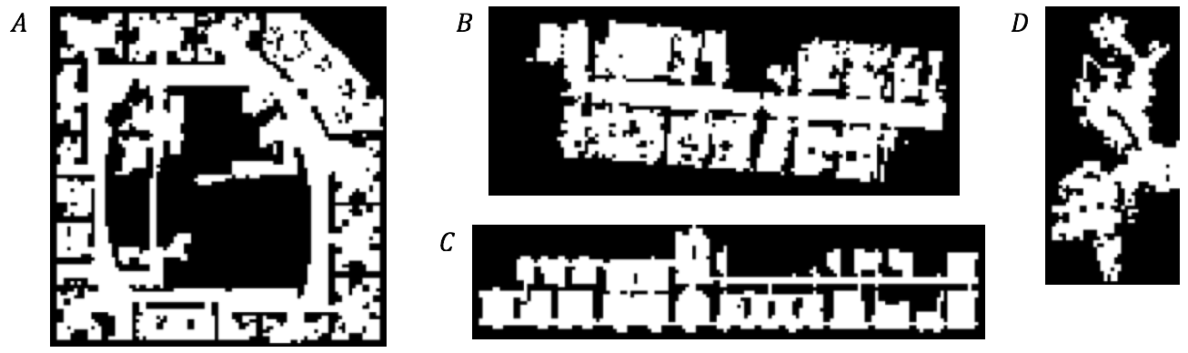
Fig. 10: Preprocessed $N\times M$ maps. A, Intel Research Lab, $100\times 101$. B, Freiburg, building 079, $139\times 57$. C, Belgioioso Castle, $151\times 35$. D, western wing of the MIT CSAIL building, $41\times 83$.

A QMDP-net policy is trained on the $30x30$-D grid navigation task on randomly generated environments. For training we set $K=90$ in the QMDP-net. We then execute the learned policy on the LIDAR maps. To account for the larger grid size we increase the number of iterations to $K=450$ when executing the policy.

C.6 Architectures for Comparison

We compare QMDP-net with two of its variants where we remove some of the POMDP priors embedded in the network (Untied QMDP-net, LSTM QMDP-net). We also compare with two generic network architectures that do not embed structural priors for decision making (CNN+LSTM, RNN). We also considered additional architectures for comparison, including networks with GRU [7] and ConvLSTM [36] cells. ConvLSTM is a variant of LSTM where the fully connected layers are replaced by convolutions. These architectures performed worse than CNN+LSTM for most of our task.

Untied QMDP-net.

We obtain Untied QMDP-net by untying the kernel weights in the convolutional layers that implement value iteration in the planner module of QMDP-net. We also remove the softmax activation on the kernel weights. This is equivalent to allowing a different transition model at each iteration of value iteration, and allowing transition probabilities that do not sum to one. In principle, Untied QMDP-net can represent the same policy as QMDP-net and it has some additional flexibility. However, Untied QMDP-net has more parameters to learn as $K$ increases. The training difficulty increases with more parameters, especially on complex domains or when training with small amount of data.

LSTM QMDP-net.

In LSTM QMDP-net we replace the filter module of QMDP-net with a generic LSTM network but keep the value iteration implementation in the planner. The output of the LSTM component is a belief estimate which is input to the planner module of QMDP-net. We first process the task parameter input $\boldsymbol{\theta}$, an image encoding the environment and goal, by a CNN. We separately process the action $\underline{a}_{t}$ and observation $\underline{o}_{t}$ input vectors by a two-layer fully connected component. These processed inputs are concatenated into a single vector which is the input of the LSTM layer. The size of the LSTM hidden state and output is chosen to match the number of states in the grid, e.g. $N^{2}$ for an $N\times N$ grid. We initialize the hidden state of the LSTM using the appropriate channel of the input $\boldsymbol{\theta}$ that encodes the initial belief.

CNN+LSTM.

CNN+LSTM is a state-of-the-art deep convolutional network with LSTM cells. It is similar in structure to DRQN [10], which was used for learning to play partially observable Atari games in a reinforcement learning setting. Note that we train the networks in an imitation learning setting using the same set of expert trajectories, and not using reinforcement learning, so the comparison with QMDP-net is fair. The CNN+LSTM network has more structure to encode a decision making policy compared to a vanilla RNN, and it is also more tailored to our input representation. We process the image input, $\boldsymbol{\theta}$, by a CNN component and the vector input, $\underline{a}_{t}$ and $\underline{o}_{t}$, by a fully connected network component. The output of the CNN and the fully connected component are then combined into a single vector and fed to the LSTM layer.

RNN.

The considered RNN architecture is a vanilla recurrent neural network with $512$ hidden units and tanh activation. At each step inputs are transformed into a single concatenated vector. The outputs are obtained by a fully connected layer with softmax activation.

We performed hyperparameter search on the number of layers and hidden units, and adjusted learning rate and batch size for all alternative networks. In particular, we ran trials for the deterministic grid navigation task. For each architecture we chose the best parametrization found. We then used the same parametrization for all tasks.

C.7 Training Technique

We train all networks, QMDP-net and alternatives, in an imitation learning setting. The loss is defined as the cross-entropy between predicted and demonstrated actions along the expert trajectories. We do not receive supervision on the underlying ground-truth POMDP models.

We train the networks with backpropagation through time on mini-batches of $100$. The networks are implemented in Tensorflow [1]. We use RMSProp optimizer [35] with $0.9$ decay rate and $0$ momentum setting. The learning rate was set to $1\times 10^{-3}$ for QMDP-net and $1\times 10^{-4}$ for the alternative networks. We limit the number of backpropagation steps to $4$ for QMDP-net and its untied variant; and to $6$ for the other alternatives, which gave slightly better results. We used a combination of early stopping with patience and exponential learning rate decay of $0.9$. In particular, we started to decrease the learning rate if the prediction error did not decrease for $30$ consecutive epochs on a validation set, $10\%$ of the training data. We performed $15$ iterations of learning rate decay.

We perform multiple rounds of the training method described above. In our partially observable domains predictions are increasingly difficult along a trajectory, as they require multiple steps of filtering, i.e. integrating information from a long sequence of observations. Therefore, for the first round of training we limit the number of steps along the expert trajectories, for training both QMDP-net and its alternatives. After convergence we perform a second round of training on the full length trajectories. Let $L_{r}$ be the number of steps along the expert trajectories for training round $r$. We used two training rounds with $L_{1}=4$ and $L_{2}=100$ for training QMDP-net and its untied variant. For training the other alternative networks we used $L_{1}=6$ and $L_{2}=100$, which gave better results.

We trained policies for the grid navigation task when the grid is fixed, only the initial state and goal vary. In this variant we found that a low $L_{r}$ setting degrades the final performance for the alternative networks. We used a single training round with $L_{1}=100$ for this task.

References

- Abadi et al. [2015] M. Abadi, A. Agarwal, P. Barham, E. Brevdo, Z. Chen, C. Citro, G. S. Corrado, A. Davis, J. Dean, M. Devin, et al. TensorFlow: Large-scale machine learning on heterogeneous systems, 2015. URL http://tensorflow.org/.
- Bagnell et al. [2003] J. A. Bagnell, S. Kakade, A. Y. Ng, and J. G. Schneider. Policy search by dynamic programming. In Advances in Neural Information Processing Systems, pages 831–838, 2003.
- Bai et al. [2010] H. Bai, D. Hsu, W. S. Lee, and V. A. Ngo. Monte carlo value iteration for continuous-state POMDPs. In Algorithmic Foundations of Robotics IX, pages 175–191, 2010.
- Bakker et al. [2003] B. Bakker, V. Zhumatiy, G. Gruener, and J. Schmidhuber. A robot that reinforcement-learns to identify and memorize important previous observations. In International Conference on Intelligent Robots and Systems, pages 430–435, 2003.
- Baxter and Bartlett [2001] J. Baxter and P. L. Bartlett. Infinite-horizon policy-gradient estimation. Journal of Artificial Intelligence Research, 15:319–350, 2001.
- Boots et al. [2011] B. Boots, S. M. Siddiqi, and G. J. Gordon. Closing the learning-planning loop with predictive state representations. The International Journal of Robotics Research, 30(7):954–966, 2011.
- Cho et al. [2014] K. Cho, B. Van Merriënboer, C. Gulcehre, D. Bahdanau, F. Bougares, H. Schwenk, and Y. Bengio. Learning phrase representations using RNN encoder-decoder for statistical machine translation. arXiv preprint arXiv:1406.1078, 2014.
- Gupta et al. [2017] S. Gupta, J. Davidson, S. Levine, R. Sukthankar, and J. Malik. Cognitive mapping and planning for visual navigation. arXiv preprint arXiv:1702.03920, 2017.
- Haarnoja et al. [2016] T. Haarnoja, A. Ajay, S. Levine, and P. Abbeel. Backprop kf: Learning discriminative deterministic state estimators. In Advances in Neural Information Processing Systems, pages 4376–4384, 2016.
- Hausknecht and Stone [2015] M. J. Hausknecht and P. Stone. Deep recurrent Q-learning for partially observable MDPs. arXiv preprint, 2015. URL http://arxiv.org/abs/1507.06527.
- Hochreiter and Schmidhuber [1997] S. Hochreiter and J. Schmidhuber. Long short-term memory. Neural Computation, 9(8):1735–1780, 1997.
- Howard and Roy [2003] A. Howard and N. Roy. The robotics data set repository (radish), 2003. URL http://radish.sourceforge.net/.
- Hsiao et al. [2007] K. Hsiao, L. P. Kaelbling, and T. Lozano-Pérez. Grasping POMDPs. In International Conference on Robotics and Automation, pages 4685–4692, 2007.
- Ji et al. [2013] S. Ji, W. Xu, M. Yang, and K. Yu. 3D convolutional neural networks for human action recognition. IEEE Transactions on Pattern Analysis and Machine Intelligence, 35(1):221–231, 2013.
- Jonschkowski and Brock [2016] R. Jonschkowski and O. Brock. End-to-end learnable histogram filters. In Workshop on Deep Learning for Action and Interaction at NIPS, 2016. URL http://www.robotics.tu-berlin.de/fileadmin/fg170/Publikationen_pdf/Jonschkowski-16-NIPS-WS.pdf.
- Krizhevsky et al. [2012] A. Krizhevsky, I. Sutskever, and G. E. Hinton. Imagenet classification with deep convolutional neural networks. In Advances in Neural Information Processing Systems, pages 1097–1105, 2012.
- Kurniawati et al. [2008] H. Kurniawati, D. Hsu, and W. S. Lee. Sarsop: Efficient point-based POMDP planning by approximating optimally reachable belief spaces. In Robotics: Science and Systems, volume 2008, 2008.
- Littman et al. [1995] M. L. Littman, A. R. Cassandra, and L. P. Kaelbling. Learning policies for partially observable environments: Scaling up. In International Conference on Machine Learning, pages 362–370, 1995.
- Littman et al. [2002] M. L. Littman, R. S. Sutton, and S. Singh. Predictive representations of state. In Advances in Neural Information Processing Systems, pages 1555–1562, 2002.
- Mirowski et al. [2016] P. Mirowski, R. Pascanu, F. Viola, H. Soyer, A. Ballard, A. Banino, M. Denil, R. Goroshin, L. Sifre, K. Kavukcuoglu, et al. Learning to navigate in complex environments. arXiv preprint arXiv:1611.03673, 2016.
- Mnih et al. [2015] V. Mnih, K. Kavukcuoglu, D. Silver, A. A. Rusu, J. Veness, M. G. Bellemare, A. Graves, M. Riedmiller, A. K. Fidjeland, G. Ostrovski, et al. Human-level control through deep reinforcement learning. Nature, 518(7540):529–533, 2015.
- Ng et al. [1999] A. Y. Ng, D. Harada, and S. Russell. Policy invariance under reward transformations: Theory and application to reward shaping. In International Conference on Machine Learning, pages 278–287, 1999.
- Okada et al. [2017] M. Okada, L. Rigazio, and T. Aoshima. Path integral networks: End-to-end differentiable optimal control. arXiv preprint arXiv:1706.09597, 2017.
- Papadimitriou and Tsitsiklis [1987] C. H. Papadimitriou and J. N. Tsitsiklis. The complexity of Markov decision processes. Mathematics of Operations Research, 12(3):441–450, 1987.
- Pineau et al. [2003] J. Pineau, G. J. Gordon, and S. Thrun. Applying metric-trees to belief-point POMDPs. In Advances in Neural Information Processing Systems, page None, 2003.
- Shani et al. [2005] G. Shani, R. I. Brafman, and S. E. Shimony. Model-based online learning of POMDPs. In European Conference on Machine Learning, pages 353–364, 2005.
- Shani et al. [2013] G. Shani, J. Pineau, and R. Kaplow. A survey of point-based POMDP solvers. Autonomous Agents and Multi-agent Systems, 27(1):1–51, 2013.
- Shankar et al. [2016] T. Shankar, S. K. Dwivedy, and P. Guha. Reinforcement learning via recurrent convolutional neural networks. In International Conference on Pattern Recognition, pages 2592–2597, 2016.
- Silver and Veness [2010] D. Silver and J. Veness. Monte-carlo planning in large POMDPs. In Advances in Neural Information Processing Systems, pages 2164–2172, 2010.
- Silver et al. [2016a] D. Silver, A. Huang, C. J. Maddison, A. Guez, L. Sifre, G. Van Den Driessche, J. Schrittwieser, I. Antonoglou, V. Panneershelvam, M. Lanctot, et al. Mastering the game of Go with deep neural networks and tree search. Nature, 529(7587):484–489, 2016a.
- Silver et al. [2016b] D. Silver, H. van Hasselt, M. Hessel, T. Schaul, A. Guez, T. Harley, G. Dulac-Arnold, D. Reichert, N. Rabinowitz, A. Barreto, et al. The predictron: End-to-end learning and planning. arXiv preprint, 2016b. URL https://arxiv.org/abs/1612.08810.
- Spaan and Vlassis [2005] M. T. Spaan and N. Vlassis. Perseus: Randomized point-based value iteration for POMDPs. Journal of Artificial Intelligence Research, 24:195–220, 2005.
- [33] C. Stachniss. Robotics 2D-laser dataset. URL http://www.ipb.uni-bonn.de/datasets/.
- Tamar et al. [2016] A. Tamar, S. Levine, P. Abbeel, Y. Wu, and G. Thomas. Value iteration networks. In Advances in Neural Information Processing Systems, pages 2146–2154, 2016.
- Tieleman and Hinton [2012] T. Tieleman and G. Hinton. Lecture 6.5 - rmsprop: Divide the gradient by a running average of its recent magnitude. COURSERA: Neural networks for machine learning, pages 26–31, 2012.
- Xingjian et al. [2015] S. Xingjian, Z. Chen, H. Wang, D.-Y. Yeung, W.-k. Wong, and W.-c. Woo. Convolutional LSTM network: A machine learning approach for precipitation nowcasting. In Advances in Neural Information Processing Systems, pages 802–810, 2015.
- Ye et al. [2017] N. Ye, A. Somani, D. Hsu, and W. S. Lee. Despot: Online POMDP planning with regularization. Journal of Artificial Intelligence Research, 58:231–266, 2017.