Inference-Based Distributed Channel Allocation
in Wireless Sensor Networks

Abstract

Interference-aware resource allocation of time slots and frequency channels in single-antenna, half-duplex radio wireless sensor networks (WSN) is challenging. Devising distributed algorithms for such task further complicates the problem. This work studies WSN joint time and frequency channel allocation for a given routing tree, such that: a) allocation is performed in a fully distributed way, i.e., information exchange is only performed among neighboring WSN terminals, within communication up to two hops, and b) detection of potential interfering terminals is simplified and can be practically realized. The algorithm imprints space, time, frequency and radio hardware constraints into a loopy factor graph and performs iterative message passing/ loopy belief propagation (BP) with randomized initial priors.

Sufficient conditions for convergence to a valid solution are offered, for the first time in the literature, exploiting the structure of the proposed factor graph. Based on theoretical findings, modifications of BP are devised that i) accelerate convergence to a valid solution and ii) reduce computation cost. Simulations reveal promising throughput results of the proposed distributed algorithm, even though it utilizes simplified interfering terminals set detection. Future work could modify the constraints such that other disruptive wireless technologies (e.g., full-duplex radios or network coding) could be accommodated within the same inference framework.

I Introduction

Designing efficient channel allocation algorithms, i.e., assigning time slots and/or frequency channels in resource constrained wireless sensor networks (WSNs), may offer tremendous interference mitigation opportunities and subsequent throughput, delay, or energy-efficiency improvements [1, 2, 3, 4, 5, 6, 7, 8, 9, 10, 11, 12]. WSNs support a wide range of applications, including environmental sensing, smart buildings, medical care, micro-climate monitoring and plethora of other industry and military applications. WSNs differ from traditional wireless ad-hoc or heterogeneous (5G) networks in the following aspects: (a) each WSN terminal is low-cost, low-power, single-antenna with half-duplex radio, (b) the number of available frequency channels in current WSNs may be limited in practice, (c) the available bandwidth of WSN terminals may be also limited, e.g., $250$ kbps in 802.15.4 networks, (d) memory and processing power are typically limited per WSN terminal, e.g., $10$ kByte memory and $8$ MHz MSP430 microcontroller in TelosB motes [13], and (e) the packet payload may be small to minimize delay and power consumption.

The problem of channel allocation becomes even more challenging in large-scale WSNs, where the computational burden should be dispensed across all terminals, pointing towards distributed protocols [3, 4, 14, 15, 5, 16, 17]. Centralized protocols may be prohibitive for large-scale WSNs with resource constrained terminals due to computation cost, as well as large delays at WSN terminals in the vicinity of the central processing unit. On the other hand, a distributed protocol requires the following: (a) local knowledge at each WSN terminal, e.g., that are its interferers [3] or its up to two-hop neighbors in the routing tree [6], and (b) a message-passing (MP) communication mechanism among neighboring terminals, based on specific synchronous or asynchronous schedule [18].

Distributed WSN frequency channel allocation algorithms are presented in [3] and [4]; in[3], a game theory-based algorithm is employed in order to minimize the total number of interfering links, while in [4], a distributed algorithm is proposed, which eliminates the remaining interference links in the WSN, by constructing a conflict-free TDMA schedule. In addition, works in [3] and [4] make the implicit assumption that interference connectivity among all WSN terminals is precisely known. Interference connectivity of a WSN terminal is defined as the set of terminals that interfere the transmission or the reception of that terminal (depending on the utilized interference set detection protocol). In many cases, the signal-to-noise ratio (SNR) at a receiving terminal $j$ may be degraded by simultaneous transmissions from a set $\mathcal{I}$ of several WSN terminals, whose individual transmission may not degrade significantly the SNR at terminal $j$; in that case, terminals in set $\mathcal{I}$ cannot be easily identified and incorporated in the interference connectivity set of terminal $j$. This is another reason why prior art has introduced the notion of interference radius, as opposed to communication radius [2].

Work in [1] calculates a TDMA schedule for packet radio networks, assuming single-frequency channel radio terminals. More specifically, constraints based on link connectivity up to two hops are encoded using a factor graph (FG), assuming that simultaneous transmission from two (or more) neighboring terminals is always harmful. Thereinafter, the loopy belief propagation (BP) runs between neighboring terminals in order to find out a global time-slot schedule that adheres to all (local) constraints.

Due to the loopy nature of the proposed FG, the mathematical toolbox to guarantee convergence to a valid solution, or even convergence to a fixed point (that may not be a valid solution) is restricted. For the latter case, only a few exemplary methodologies and results exist in the literature [19, 20, 21, 22, 23, 24, 25, 26, 27, 28]. In a general loopy probabilistic graphical model (PGM), where BP is executed, convergence to a fixed point does not necessarily imply correctness, i.e., convergence to a valid (or correct) solution, apart from special cases, as in Gaussian BP [19] or maximum weight matching problems [25, 26]; convergence to a correct solution is a critical part in our channel allocation challenge, crafted as a feasibility problem.

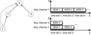
Figure 1: Transmissions of WSN terminals under two channel allocation schemes, for the the specific routing tree (solid lines) and specific interference link (dotted line). Top allocation is based on time slots, bottom allocation is based on both time slots and frequency channels. This work offers such allocations with distributed inference, under convergence, correctness and computation cost guarantees.

On the other hand, joint time and frequency channel allocation accounts not only for time but also for frequency channelization, which is an essential part of contemporary multi-channel radio modules, as it provides additional degrees of freedom and thus, potential for more efficient networking. For example, consider the $4$-terminal network of Fig. 1 with the specific routing tree topology (solid lines) and two channel allocation schemes, one with time slots (top) and a second with both time and frequency channels (bottom); under single-frequency half-duplex radios, $3$ time slots are needed so that information from the leaf terminals reaches sink terminal $4$ (top allocation); that is due to the fact that transmission of terminal $1$ towards parent terminal $3$ is interfering receiver $4$ (and such interfering link between $1$ and $4$ is depicted as a dotted line in Fig. 1). With multiple frequency channels, the required time slots are reduced to $2$ (bottom allocation), even with half-duplex radios, offering smaller delay and higher effective throughput, at the expense of additional bandwidth.

From an implementation point of view, identification of potential interferers, i.e., interference set detection, is a prerequisite step for any joint time-frequency allocation algorithm. In addition to the above, single-antenna, half-duplex radios impose extra hardware constraints that have to be taken into account, rendering time slot and frequency channel allocation a challenging task for WSNs.

This work extends time slot allocation in [1] and addresses distributed, joint time slot and frequency channel allocation. Following the RID framework in [10], practical, low-complexity interference set detection is utilized, based on signal-to-noise-and-interference ratio (SINR). In addition, a routing tree is assumed, as in well-known WSN protocols [29, 30, 31], with sink as the tree root. The proposed algorithm is a modified version of loopy BP running on a carefully crafted FG that encodes both time and frequency-based constraints, taking into account routing and interference connectivity, as well as radio hardware constraints, e.g., due to half-duplex operation or the fact that each radio can tune at a single frequency channel at a time. Each WSN terminal is associated with specific variables and factor nodes of the FG, so that message passing (MP) with neighboring WSN terminals in communication connectivity is only needed. The MP schedule of the proposed FG requires the transmission of a single real number per directed FG edge and can be implemented in a distributed manner. The objective is to find a feasible frequency-time allocation that adheres to specific communication, routing, interference and radio hardware constraints.

The contributions of this work are summarized below:

1. A joint time slot and frequency channel allocation algorithm is offered, based on loopy BP; the algorithm is distributed, since each WSN terminal needs to communicate with up to two-hop neighboring WSN terminals in communication radius (i.e., communication connectivity), associated with routing and interference. Interference set detection is practical and based on sensitivity and SINR at each receiving radio terminal.

2. Sufficient conditions for convergence to correct solution are offered for loopy BP, for the first time in the literature (to the best of our knowledge), exploiting the structure of the underlying PGM; the latter is crafted under the specific problem constraints.

3. Computation cost reduction methods are offered, based on precomputed feasibility sets found with binary search; such methodology is important since the complexity of the underlying loopy BP algorithm is exponential in the PGM degree, which in turn depends on network connectivity.

4. An interesting tradeoff is offered between remaining interference of the offered solution and computation time. Furthermore, random local re-initialization among WSN terminals running the algorithm is introduced, showing significant convergence acceleration.

The inherent expressive power of MP/BP inference framework, including asynchronous scheduling capabilities, could spark interest for distributed solutions in other network scenarios, offering perhaps a new, fresh look at an old networking problem [32, 33]. Compared to conference version [34], this work provides a detailed exposition of the adopted interference set detection procedure, offers new sufficient convergence conditions on exact solution (with proof), examines complexity issues and proposes acceleration techniques; in addition, numerical results study large-scale WSN topologies and quantify how quickly the proposed algorithm converges to an exact solution under fully distributed operation using the proposed modification of BP.

Notation: Symbol $\mathcal{U}[0,1]$ denotes the continuous uniform distribution over the (closed) interval $[0,1]$. Symbols $\mathds{B}$ and $\mathds{N}\triangleq\{1,2,\ldots\}$ denote the set of binary and natural numbers, respectively. The operator $|\cdot|$ stands for the cardinality of a set, i.e., $|\mathds{B}|=2$. The number of the non-zero elements of a vector $\mathbf{x}$, is denoted $\|\mathbf{x}\|_{0}$. The vector comprised of variables associated with an arbitrary index set $\mathcal{A}$, is denoted as $\mathbf{x}_{\mathcal{A}}=\left\{x_{y}\right\}_{y\in\mathcal{A}}$. Symbol $\mathsf{1}\{\cdot\}$ stands for the indicator function that returns one if the statement within the brackets is true, and zero, otherwise.

II Problem Formulation and Interferer Set Detection

A WSN consisting of $N$ single-antenna, half-duplex radio terminals is considered. Sink terminal operates in receiver mode only. A terminal needs a time slot to transmit a packet and each transmission frame consists of $M$ equal-length time slots. The available frequency bandwidth is divided into $K$ orthogonal frequency channels. Let $\mathcal{M}\triangleq\{1,2,\ldots,M\}$ and $\mathcal{K}\triangleq\{1,2\ldots,K\}$ be the set of available time slots and frequency channels, respectively. Let $\mathcal{N}$ be the set of all terminals in the WSN (sink included); a communication link $(i,j)$ between two terminals $i,j\in\mathcal{N}$ exists if during $i$’s transmission, the received signal strength at terminal $j$ is above its receiver sensitivity.

TABLE I: Notation and Relations in WSN Routing Tree

Symbol	Relations in WSN routing tree connectivity
$\mathcal{N}$	all WSN terminals, i.e., $\mathcal{N}\triangleq\{1,\ldots,N\}$
$\mathtt{s}$	the sink terminal, $\mathtt{s}\in\mathcal{N}$
$\mathcal{N}_{\backslash\mathtt{s}}$	all WSN terminals except sink, i.e., $\mathcal{N}_{\backslash\mathtt{s}}\triangleq\mathcal{N}\backslash\mathtt{s}$
${\rm par}(i)$	the (unique) parent of terminal $i$
$\mathcal{N}_{\rm ch}(i)$	children of terminal $i$: $\mathcal{N}_{\rm ch}(i)\triangleq\left\{i^{\prime}\in\mathcal{N}:{\rm par}\!\left(i^{\prime}\right)=i\right\}$
$\mathcal{N}_{\rm sib}(i)$	the set of sibling terminals of terminal $i$, i.e.,
	$\mathcal{N}_{\rm sib}(i)\triangleq\left\{i^{\prime}\in\mathcal{N}_{\backslash\mathtt{s}}\backslash i:i^{\prime}\in\mathcal{N}_{\rm ch}\!\left({\rm par}\!\left(i^{\prime}\right)\right)\right\}$
$\mathcal{N}_{\rm OneH}(i)$	the set of one-hop neighbors of terminal $i$, i.e.,
	$\mathcal{N}_{\rm OneH}(i)\triangleq\big{\{}i^{\prime}\in\mathcal{N}_{\backslash\mathtt{s}}:i^{\prime}\in\mathcal{N}_{\rm ch}(i)\cup i~{}\cup$ ${\rm par}(i)\big{\}}$
	the set of two-hop neighbors of terminal $i$, i.e.,
$\mathcal{N}_{\rm TwoH}(i)$	$\mathcal{N}_{\rm TwoH}(i)\!\triangleq\!\bigg{\{}i^{\prime}\in\mathcal{N}_{\backslash\mathtt{s}}\!:\!i^{\prime}\in\mathcal{N}_{\rm OneH}({\rm par}(i))\cup$
	$\left(\bigcup_{j\in\mathcal{N}_{\rm ch}(i)}\mathcal{N}_{\rm OneH}(j)\right)\bigg{\}}$

A tree routing connectivity is assumed [35], abbreviated as $\mathcal{T}=(\mathcal{N},\mathcal{C}_{\mathcal{T}})$, where $\mathcal{C}_{\mathcal{T}}$ is the set of the edges of the WSN routing tree after the execution of routing algorithm. Table I summarizes the adopted notation related to the routing connectivity (for exposition purposes the defined sets exclude sink terminal $\mathtt{s}$).

For any routing link $(i,j)\in\mathcal{C}_{\mathcal{T}}$, (i.e., $j={\rm par}(i)$), the set of potential interferers of link $(i,j)$ consists of any subset $\mathcal{I}$ of terminals that degrade the signal-to-noise-ratio (SNR) at receiver $j$; in other words, WSN terminals in $\mathcal{I}$ satisfying

$${\rm SINR}_{i\rightarrow j}^{\mathcal{I}}=\frac{P_{i}|{h}_{i,j}|^{2}}{\sigma_{j}^{2}+\sum_{i^{\prime}\in\mathcal{I}}P_{i^{\prime}}|{h}_{i^{\prime},j}|^{2}}<\theta,$$ (1)

should be included in the set of links’ $(i,j)$ potential interferers. In Eq. (1), $P_{i}$ is the power of transmitter $i$, ${h}_{i,j}$ is the instantaneous channel gain coefficient between transmitter $i$ and receiver $j$ incorporating both large and small scale fading, $\sigma_{j}^{2}$ is the thermal noise power at receiver $j$, and $\theta$ is a threshold parameter that depends on the receiver sensitivity. Executing the SINR test in Eq. (1), requires a search on all possible subsets of interfering terminals, which is prohibitive for resource constrained WSN terminals. More importantly, discovery of interfering terminals may be impossible, since a WSN terminal may contribute to the sum of the denominator in Eq. (1), but with power which may not be adequate for receiver $j$ to properly decode a packet and discover the identity of the interferer; the superposition of several undecodable signals can contribute to the the sum in the denominator of Eq. (1).

Even though modeling of interference in this work adheres to Eq. (1) (utilized also during numerical results), discovery of interfering terminals adopts a modified version of lightweight RID protocol [10], simplifying interference set identification. Let us denote $\mathcal{N}_{\rm pint}(j)$ the set of potential interferers of terminal $j$, including all WSN terminals $i^{\prime}$ satisfying the following conditions: a) link between $i^{\prime}$ and $j$ does not belong to the routing tree (i.e., $(i^{\prime},j)\notin\mathcal{C}_{\mathcal{T}}$) and b) reception of $i^{\prime}$ transmission at $j$ is above $j$’s receiver sensitivity. Terminal $i^{\prime}\in\mathcal{N}_{\rm pint}(j)$ is an actual interferer of transmission from child $i$ to parent $j$ (or simply interferer of $j$), if the following condition holds

$${\rm SINR}_{i\rightarrow j}^{i^{\prime}}=\frac{P_{i}|{h}_{i,j}|^{2}}{\sigma_{j}^{2}+P_{i^{\prime}}|{h}_{i^{\prime},j}|^{2}}<\theta.$$ (2)

Link between terminal $i^{\prime}$ and $j$ is an interfering link. Discovery of interferes for a specific link (or equivalently for a specific receiver) requires examination of the above test for all terminals $i^{\prime}\in\mathcal{N}_{\rm pint}(j)$. Examination of the above test requires linear complexity on the number of potential interferers. This simplification, even though underestimates the number of potential interferers, reduces the required overhead needed for interfering set identification. Moreover, the above test can be practically applied among WSN terminals neighboring to $j$, that can be properly decoded and identified by $j$.

Let $\mathcal{I}_{\rm interf}(i)$ denote the set of terminals that interfere the transmission of child $i$ to its parent using the test in (2). For exposition purposes, set $\mathcal{I}_{\rm interf}(i)$ also includes child $i$ itself, $i$’s parent, and excludes sink terminal:

$$\mathcal{I}_{\rm interf}(i)\triangleq ~{}\bigg{\{}\bigg{\{}i^{\prime}\in\mathcal{N}_{\rm pint}(j):{\rm SINR}_{i\rightarrow{\rm par}(i)}^{i^{\prime}}<\theta\bigg{\}}$$

$$\cup i\cup{\rm par}(i)\bigg{\}}\big{\backslash}\mathtt{s}.$$ (3)

For example, consider the network of Fig. 2 and a threshold $\theta$ such that ${\rm SINR}_{3\rightarrow 4}^{1}<\theta$ and ${\rm SINR}_{5\rightarrow 4}^{1}<\theta$, i.e., both children $3$ and $5$ are disturbed from terminal’s $1$ simultaneous transmission. It is noted that $\mathcal{N}_{\rm pint}(5)=\{1\}$, while $\mathcal{N}_{\rm pint}(3)=\emptyset$, because link $(1,3)$ exists in routing connectivity. According to Eq. (3), $\mathcal{I}_{\rm interf}(1)=\{1,3\}$, $\mathcal{I}_{\rm interf}(2)=\{2,3\}$, $\mathcal{I}_{\rm interf}(3)=\{1,3\}$, $\mathcal{I}_{\rm interf}(4)=\emptyset$ and $\mathcal{I}_{\rm interf}(5)=\{1,5\}$. Also, note that WSN terminals $1$ and $5$ are connected within two hops, since $1$ and $4$ (parent of $5$) are in communication range, according to the interferer set detection criteria in Eq. (2) and WSN terminals $4$ and $5$ have a parent-child routing connection. It is emphasized again that while interference set detection is simplified according to the above, performance evaluation of the proposed time slot and frequency channel allocation algorithm will be conducted taking into account all interferers in Eq. (1) and not just the detected ones.

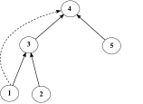
Figure 2: A simple WSN routing tree with $5$ sensor terminals. Dashed and solid lines depict interference and routing connectivity, respectively. Terminal 1 interferes reception at terminal 4 (or transmission of terminal 5), even though it transmits to terminal 3 only.

A key attribute of the proposed scheme is that specific routing tree connectivity is assumed. The routing tree provides extra structure and knowledge to the WSN that can be exploited by any WSN terminal. This (spatial) structure imposes specific child-parent connections (Fig. 2) that impose further design constraints:

• Siblings cannot transmit to their parent at the same time slot.

• A child and its parent cannot transmit at the same time slot (due to the half-duplex constraint).

• A WSN terminal can tune at a single carrier frequency and transmit at a single frequency channel (out of $K$) at a given time slot.

• A WSN terminal has knowledge of its up to $2$-hop neighbors. Furthermore, neighbors within exactly $2$-hops cannot transmit at the same time slot and at the same frequency channel (due to the hidden terminal problem). It is remarked that in the latter case they could utilize different frequency channels.

The above constraints assume a routing tree and will be summarized as routing connectivity constraints.

Interference is caused to a parent terminal receiver, when a single or multiple terminals (that are not children of the specific parent in the routing tree) are transmitting at the same time slot and at the same frequency channel and the SINR at the parent receiver, as defined in Eq. (2), is below a predetermined threshold $\theta$; otherwise, the specific transmitter(s) will cause no interference:

• When a child transmits and there exists at least one interfering simultaneous transmission, the interfering terminal(s) and the child terminal must be assigned different frequency channels for a given time slot.

The above constraint is due to interference connectivity. Constraint 5. along with 2. and 3. constitute the interference connectivity constraints. When more than one interfering terminals are discovered, then they must be allocated to different frequency channels.

Finally, the algorithm should consider that each terminal should transmit once during a specific frame (of $M$ time slots, as described above):

• A WSN terminal transmits during exactly one time slot per transmission frame (with the exception of the sink which always receives).

The above constraint will be referenced as the transmission constraint.

The above criteria can be easily modified to accommodate modern wireless transmission technologies, such as those based on full-duplex radios or network coding, left for future work. This work solves the following problem: given the above set of constraints, as well as a given routing tree and a specific set of (practically discovered) interferers, offer an inference algorithm that allows all WSN terminals to discover channel allocation (both in terms of time and frequency resources) that adheres to the constraints, while each WSN terminal exchanges information with up to two-hop neighbors in communication connectivity. Such distributed algorithm is accompanied with convergence and correctness guarantees, while computation costs are also meticulously taken into account.

III Distributed Joint Time/Frequency Allocation FG Algorithm

III-A Factor Graph Modeling

The factor graph (FG) construction requires random variables, whereas their factor nodes check their dependencies and implement the constraints of the initial problem. The dependencies between the random variables could be also offered in terms of a matrix description, that resembles the parity check matrix in factor graph-based coding literature (e.g., [36, 37]). Towards that goal, a set of binary variables $\left\{s_{i,m}^{(k)}\right\}$ is defined, with $i\in\mathcal{N}_{\backslash\mathtt{s}},\;m\in\mathcal{M},\;k\in\mathcal{K}$. Binary variable $s_{i,m}^{(k)}$ is called scheduling variable of terminal $i$ (excluding sink terminal) and denotes transmission ($s_{i,m}^{(k)}=1$) or no transmission $(s_{i,m}^{(k)}=0)$ of transmitter $i$, at time slot $m$ and frequency channel $k$.

Each constraint variable is input to specific factor nodes that check the validity of specific constraints and return $1$ if the constraints are satisfied and $0$, otherwise. Given that there are three kinds of (local) constraints (i.e., routing, interference, and transmission), three kinds of factor nodes are constructed:

• $\mathsf{f}$ factors (or routing factors): each $\mathsf{f}_{i,m}$ factor node is related to terminal $i\in\mathcal{N}$ at time slot $m$ and checks the validity of routing connectivity constraints. The domain of each factor $\mathsf{f}$ is given by

  $$\mathbf{dom}\mathsf{f}_{i,m}= \left\{\left\{s_{i^{\prime},m}^{(k^{\prime})}\in\mathds{B}\right\}:i^{\prime}\in\mathcal{N}_{\rm TwoH}(i),\;k^{\prime}\in\mathcal{K}\right\}$$

  $$= ~{}\mathds{B}^{|\mathcal{N}_{\rm TwoH}(i)|K}.$$ (4)

• $\mathsf{h}$ factors (or interference factors): similarly, each $\mathsf{h}_{i,m}$ factor node is related to terminal $i\in\mathcal{N}_{\backslash\mathtt{s}}$ at time slot $m$ and checks the validity of interference connectivity constraints. The domain of each factor $\mathsf{h}$ is given by

  $$\mathbf{dom}\mathsf{h}_{i,m}= \left\{\left\{s_{i^{\prime},m}^{(k^{\prime})}\in\mathds{B}\right\}:i^{\prime}\in\mathcal{I}_{\rm interf}(i),\;k^{\prime}\in\mathcal{K}\right\}$$

  $$= ~{}\mathds{B}^{|\mathcal{I}_{\rm interf}(i)|K}.$$ (5)

• $\mathsf{t}$ factors (or transmission factors): for each terminal but sink there exists a corresponding $\mathsf{t}_{i}$ factor, $i\in\mathcal{N}_{\backslash\mathtt{s}}$, which is related to the validity of the transmission constraints. The domain is given by

  $$\mathbf{dom}\mathsf{t}_{i}=\left\{\left\{s_{i,m^{\prime}}^{(k^{\prime})}\in\mathds{B}\right\}:m^{\prime}\in\mathcal{M},\;k^{\prime}\in\mathcal{K}\right\}=\mathds{B}^{KM}.$$ (6)

Each WSN terminal (except sink) has $2M+1$ (local) factor nodes and $MK$ variables nodes; specifically, for each $i\in\mathcal{N}_{\backslash\mathtt{s}}$, there are $M$ routing connectivity factors ($\mathsf{f}_{i,m},\;\forall m\in\mathcal{M}$), $M$ interference connectivity factors ($\mathsf{h}_{i,m},\;\forall m\in\mathcal{M}$) and one transmission factor ($\mathsf{t}_{i}$). The sink terminal has $M$ factors and no variables. Detailed description of $\mathsf{f,h}$ and $\mathsf{t}$ factors is offered at Appendix A.

A few factor domain examples are given for the network of Fig. 2 with $M=2$ time slots and $K=2$ frequency channels:

$$\mathbf{dom}\mathsf{f}_{4,1}\! ~{}=\left\{\mathds{B}^{8}\ni\left[s_{1,1}^{(1)}~{}s_{2,1}^{(1)}~{}s_{3,1}^{(1)}~{}s_{5,1}^{(1)}~{}s_{1,1}^{(2)}~{}s_{2,1}^{(2)}~{}s_{3,1}^{(2)}~{}s_{5,1}^{(2)}\right]\right\},$$

$$\mathbf{dom}\mathsf{h}_{5,2}\! ~{}=\left\{\mathds{B}^{4}\ni\left[s_{1,2}^{(1)}~{}s_{5,2}^{(1)}~{}s_{1,2}^{(2)}~{}s_{5,2}^{(2)}\right]\right\},$$ (7)

$$\mathbf{dom}\mathsf{t}_{3}\! ~{}=\left\{\mathds{B}^{4}\ni\left[s_{3,1}^{(1)}~{}s_{3,2}^{(1)}~{}s_{3,1}^{(2)}~{}s_{3,2}^{(2)}\right]\right\}.$$

Do note that the domain of interference connectivity factor $\mathsf{h}_{5,2}$ includes binary variables $s_{5,2}^{(1)}$ and $s_{5,2}^{(2)}$ of WSN terminal $5$ itself. Also notice that the same domain of WSN terminal $5$ includes variables from WSN terminal $1$, which is connected to $5$ in the physical WSN topology within two hops, due to interference connectivity, explained in the previous section II. In the FG bipartite topology, factor $\mathsf{h}_{5,2}$ belongs to WSN terminal $5$ and is connected within 1 hop to variables $s_{1,2}^{(1)},s_{1,2}^{(2)}$ that belong to WSN terminal $1$. As an additional example, consider an arbitrary input configuration for factor $\mathsf{f}_{4,1}$, e.g., $\left[s_{1,1}^{(1)}~{}s_{2,1}^{(1)}~{}s_{3,1}^{(1)}~{}s_{5,1}^{(1)}~{}s_{1,1}^{(2)}~{}s_{2,1}^{(2)}~{}s_{3,1}^{(2)}~{}s_{5,1}^{(2)}\right]=[1~{}0~{}0~{}0~{}0~{}0~{}0~{}1]$, which simply states that terminals $1$ and $5$ transmit simultaneously at time slot $1$, at different frequency channels; hence $\mathsf{f}_{4,1}([1~{}0~{}0~{}0~{}0~{}0~{}0~{}1])=1$, since no routing connectivity constraint is violated from the perspective of terminal $4$ at time slot $1$. Similarly, consider the local factor $\mathsf{h}_{5,2}$, with configuration $[s_{1,2}^{(1)}~{}s_{5,2}^{(1)}~{}s_{1,2}^{(2)}~{}s_{5,2}^{(2)}]$ $=[1~{}0~{}0~{}1]$, which indicates that terminals $1$ and $5$ both transmit at time slot $2$, at different frequency channels; thus, the reception of $4$ is not interfered, hence $\mathsf{h}_{5,2}([1~{}0~{}0~{}1])=1$.

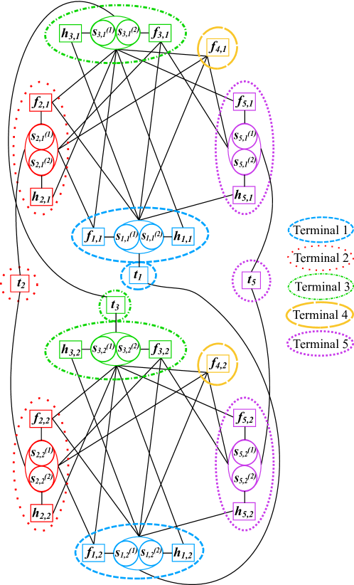
Figure 3: The factor graph (FG) corresponding to the WSN of Fig. 2 for $M=2$ time slots and $K=2$ frequency channels. For presentation purposes each depicted hyper-variable incorporates two variables and each depicted hyper-edge incorporates two edges.

For each WSN terminal, the scheduling variables are constructed and connected to the local routing connectivity, interference connectivity, and transmission constraint factors. The goal is to find a proper time slot and frequency channel allocation that adheres to all constraints; that is equivalent to construct a FG with factorization that satisfies

$$\left(\prod_{i\in\mathcal{N}_{\backslash\mathtt{s}}}\mathsf{t}_{i}(\mathbf{s}_{\mathsf{t}_{i}})\right)\cdot\left(\prod_{m\in\mathcal{M}}\left(\prod_{i\in\mathcal{N}_{\backslash\mathtt{s}}}\mathsf{h}_{i,m}\!\!\left(\mathbf{s}_{\mathsf{h}_{i,m}}\right)\right)\cdot\right.$$

$$~{}~{}~{}~{}~{}~{}~{}~{}~{}~{}~{}~{}~{}~{}~{}~{}~{}~{}~{}~{}~{}~{}~{}~{}~{}~{}~{}~{}~{}~{}~{}\cdot\left.\left(\prod_{i\in\mathcal{N}}\mathsf{f}_{i,m}\!\!\left(\mathbf{s}_{\mathsf{f}_{i,m}}\right)\right)\right)=1,$$ (8)

where $\mathbf{s}_{\mathsf{t}_{i}},\mathbf{s}_{\mathsf{f}_{i,m}}$, and $\mathbf{s}_{\mathsf{h}_{i,m}}$ denote the variable subsets of the corresponding factors. The appropriate value of $M$ depends on the overall (routing and interference) network connectivity, as well as the amount of traffic. In this work, $M$ is assumed fixed and chosen as the maximum node degree of the routing tree. When the specific choice of $M$ does not offer a valid solution, it is increased by one until a valid solution is found. The FG of Fig. 3 corresponds to the network of Fig. 2 for $M=2$, $K=2$ and interference connectivity according to ${\rm SINR}_{3\rightarrow 4}^{1}<\theta$, ${\rm SINR}_{5\rightarrow 4}^{1}<\theta$. Factor definitions offer two useful propositions that will be exploited subsequently:

Proposition 1.

For $\mathsf{f}_{i,m}$ factors, the variable assignments satisfying $\left\|\mathbf{s}_{\mathsf{f}_{i,m}}\right\|_{0}\geq|\mathcal{N}_{\rm TwoH}(i)|$ offer $\mathsf{f}_{i,m}\!\left(\mathbf{s}_{\mathsf{f}_{i,m}}\right)=0$.

Proof.

This can be shown by translating $\left\|\mathbf{s}_{\mathsf{f}_{i,m}}\right\|_{0}\geq|\mathcal{N}_{\rm TwoH}(i)|$ in terms of WSN routing connectivity as follows: if $\left\|\mathbf{s}_{\mathsf{f}_{i,m}}\right\|_{0}\geq|\mathcal{N}_{\rm TwoH}(i)|$ then either (a) all $2$-hop neighbors of $i$ in routing tree (including its child or its parent or both) transmit at the same time-slot and the same frequency channel, which is inappropriate due to constraint $2$. or (b) some terminals in the routing tree’s $2$-hop neighborhood of terminal $i$ transmit at more than $1$ frequency channels concurrently, which is inappropriate due to constraint $3$. ∎

Proposition 2.

For $\mathsf{h}_{i,m}$ factors, the variable assignments satisfying $\left\|\mathbf{s}_{\mathsf{h}_{i,m}}\right\|_{0}\geq\min\left\{K+1,|\mathcal{I}_{\rm interf}(i)|\right\}$ offer $\mathsf{h}_{i,m}\!\left(\mathbf{s}_{\mathsf{h}_{i,m}}\right)=0$.

Proof.

If $|\mathcal{I}_{\rm interf}(i)|\leq K+1\leq\left\|\mathbf{s}_{\mathsf{h}_{i,m}}\right\|_{0}$, then either (a) interference neighbors (including node $i$) transmit concurrently with $i$’s parent, which is inappropriate according to constraint 2. and constraint 5. or (b) some of terminal’s $i$ interferers transmit at more than $1$ frequency channels concurrently, which is inappropriate according to constraint 3. If $\left\|\mathbf{s}_{\mathsf{h}_{i,m}}\right\|_{0}\geq|\mathcal{I}_{\rm interf}(i)|>K+1$, at most $K$ frequency channels have been assigned to at least $K+2$ terminals; that is inappropriate due to constraint 3. ∎

III-B Proposed Synchronous Loopy BP

For exposition purposes of the loopy BP algorithm, simplified notation for variable and factor nodes is adopted. Specifically, the set of variables is relabeled as:

$$\left\{s_{i,m}^{(k)}:i\in\mathcal{N}_{\backslash\mathtt{s}},m\in\mathcal{M},k\in\mathcal{K}\right\}\!\triangleq\!\{x_{1},x_{2},\ldots,x_{MK(N-1)}\}$$ (9)

and each variable is indexed by elements in the following set:

$$\mathcal{V}\triangleq\{1,2,\ldots,MK(N-1)\}.$$ (10)

In that way, for every $v\in\mathcal{V}$ there exist unique $i\in\mathcal{N}_{\backslash\mathtt{s}}$, $m\in\mathcal{M}$ and $k\in\mathcal{K}$, such that $x_{v}=s_{i,m}^{(k)}$.

Moreover, the set of factors is relabeled as follows:

$$\left\{\left\{\mathsf{f}_{i,m}\right\}_{(i,m)\in\mathcal{N}\times\mathcal{M}},\left\{\mathsf{h}_{i,m}\right\}_{(i,m)\in\mathcal{N}_{\backslash\mathtt{s}}\times\mathcal{M}},\left\{\mathsf{t}_{i}\right\}_{i\in\mathcal{N}_{\backslash\mathtt{s}}}\right\}$$

$$\triangleq ~{}\{\mathsf{g}_{J}\}_{J=1}^{(N-1)(2M+1)+M}.$$ (11)

We index the set of factors as follows:

$$\mathcal{J}\triangleq\{1,2,\ldots,(N-1)(2M+1)+M\}.$$ (12)

As a result, for any factor $\mathsf{g}_{J}$, $J\in\mathcal{J}$, there exist unique $i\in\mathcal{N}$ and $m\in\mathcal{M}$ such that $\mathsf{g}_{J}=\mathsf{f}_{i,m}$, or unique $i\in\mathcal{N}_{\backslash\mathtt{s}}$ and $m\in\mathcal{M}$ such that $\mathsf{g}_{J}=\mathsf{h}_{i,m}$, or unique $i\in\mathcal{N}_{\backslash\mathtt{s}}$ such that $\mathsf{g}_{J}=\mathsf{t}_{i}$. A variable $x_{v},v\in\mathcal{V}$, is an argument in factor $\mathsf{g}_{J},J\in\mathcal{J}$, if and only if, $x_{v}$ is adjacent to $\mathsf{g}_{J}$ in the FG. The neighborhood of index variable $v\in\mathcal{V}$ and index factor $J\in\mathcal{J}$ in the FG is defined as follows:

$$\mathcal{J}_{v} \triangleq\{J\in\mathcal{J}:\text{variable $x_{v}$ is adjacent to factor $\mathsf{g}_{J}$}\},$$ (13)

$$\mathcal{V}_{J} \triangleq\{v\in\mathcal{V}:\text{variable $x_{v}$ is adjacent to factor $\mathsf{g}_{J}$}\},$$ (14)

respectively.

The messages at iteration $n$ from variable nodes to factor nodes and vice versa are denoted by $\mathsf{m}^{(n)}_{v\rightarrow J}(x_{v})$ and $\mathsf{m}^{(n)}_{J\rightarrow v}(x_{v})$, respectively. The proposed algorithm initializes independently each message $\mathsf{m}^{(0)}_{v\rightarrow J}(0)=1-\mathsf{m}^{(0)}_{v\rightarrow J}(1)=q_{v}$, with $q_{v}\sim\mathcal{U}[0,1]$ and $\mathsf{m}^{(0)}_{J\rightarrow v}(0)=\mathsf{m}^{(0)}_{J\rightarrow v}(1)=0$. Parameter $q_{v}$ can be considered as the initial random guess (prior) of the corresponding scheduling variable being 0, i.e., $\text{P}_{v}(0)=q_{v}=1-\text{P}_{v}(1)$ (where $\text{P}_{v}(x),\;x\in\mathds{B}$, is the prior probability distribution function of binary variable $x_{v},\;v\in\mathcal{V}$). For each $n\in\mathds{N}$, the standard BP update rules follow [38, 39]:

$$\mathsf{m}^{(n)}_{J\rightarrow v}(x_{v}) =\mathtt{C}_{J\rightarrow v}^{(n)}(\mathbf{q})\!\!\!\!\!\sum_{\mathbf{x}_{\mathcal{V}_{J}\backslash{v}}\in\mathds{B}^{|\mathcal{V}_{J}|-1}}\!\!\!\mathsf{g}_{J}(\mathbf{x}_{\mathcal{V}_{J}})\!\!\prod_{{y}\in\mathcal{V}_{J}\backslash v}\!\!\mathsf{m}^{(n-1)}_{{y}\rightarrow J}(x_{y}),$$ (15)

$$\mathsf{m}^{(n)}_{v\rightarrow J}(x_{v}) =\mathtt{C}_{v\rightarrow J}^{(n)}(\mathbf{q})~{}\text{P}_{v}(x_{v})\prod_{I\in\mathcal{J}_{v}\backslash J}\mathsf{m}^{(n)}_{{I}\rightarrow v}(x_{v}),$$ (16)

where constants $\mathtt{C}_{J\rightarrow v}^{(n)}(\mathbf{q})$ and $\mathtt{C}_{v\rightarrow J}^{(n)}(\mathbf{q})$ guarantee that $\mathsf{m}^{(n)}_{J\rightarrow v}(0)+\mathsf{m}^{(n)}_{J\rightarrow v}(1)=1$ and $\mathsf{m}^{(n)}_{v\rightarrow J}(0)+\mathsf{m}^{(n)}_{v\rightarrow J}(1)=1$, respectively; their value depends on a subset of priors $\mathbf{q}=[q_{1}~{}q_{2}~{}\ldots~{}q_{{MK(N-1)}}]\in[0,1]^{MK(N-1)}$, as well as the current iteration. By the definition of $\mathbf{q}\subset[0,1]^{MK(N-1)}$, it can be shown inductively that $\mathtt{C}_{J\rightarrow v}^{(n)}(\mathbf{q})\geq 1$ and $\mathtt{C}_{v\rightarrow J}^{(n)}(\mathbf{q})\geq 1$, $\forall n\in\mathds{N}$. For any variable assignment $\mathbf{x}_{\mathcal{V}_{J}}\in\mathds{B}^{|\mathcal{V}_{J}|}=\mathbf{dom}\mathsf{g}_{J}$, factor $\mathsf{g}_{J}$ returns either one or zero. Notation $\mathbf{x}_{\mathcal{V}_{J}\backslash v}\in\mathds{B}^{|\mathcal{V}_{J}|-1}$ under the summation indicates sum over all possible binary configurations of the variables in vector $\mathbf{x}_{\mathcal{V}_{J}}$ except variable $x_{v}$. It is also noted that each message along an edge $(J,v)$ or $(v,J)$ can be parameterized by a single real number.

In addition, a damping technique can be employed to decrease the probability of divergence [21, 40, 41]. Specifically, after the calculation of messages from factors to variables in Eq. (15), the following damping step is utilized:

$$\mathsf{m}^{(n)}_{J\rightarrow v}(x_{v})=\alpha^{(n)}\mathsf{m}^{(n-1)}_{J\rightarrow v}(x_{v})\!+\!\left(1-\alpha^{(n)}\!\right)\mathsf{m}^{(n)}_{J\rightarrow v}(x_{v}),$$ (17)

with $\alpha^{(n)}\in[0,1),\;\forall n\in\mathds{N}$. Finally, marginals, denoted as ${\mathsf{r}}_{v}^{(n)}(x_{v}),~{}\forall v\in\mathcal{V}$, determine the final values of the scheduling random variables:

$$\mathsf{r}_{v}^{(n)}(x_{v})=\text{P}_{v}(x_{v})\prod_{J\in\mathcal{J}_{v}}\mathsf{m}^{(n)}_{J\rightarrow v}(x_{v}).$$ (18)

The value of each variable at iteration $n$ is inferred using the following rule:

$$\widehat{x}^{(n)}_{v}=\mathsf{1}\!\left\{\mathsf{r}_{v}^{(n)}(1)\geq\mathsf{r}_{v}^{(n)}(0)\right\},~{}~{}\forall v\in\mathcal{V}.$$ (19)

Denote $\widehat{\mathbf{x}}^{(n)}\triangleq\left\{\widehat{x}^{(n)}_{v}\right\}_{v\in\mathcal{V}}$ and define the following:

$$\mathsf{FG}\!\left(\widehat{\mathbf{x}}^{(n)}\right)\triangleq\prod_{J\in\mathcal{J}}\mathsf{g}_{J}\!\left(\widehat{\mathbf{x}}^{(n)}_{\mathcal{V}_{J}}\right).$$ (20)

In a centralized implementation the algorithm terminates at the first iteration index $n^{\star}$, for which $\mathsf{FG}\!\left(\widehat{\mathbf{x}}^{(n^{\star})}\right)=1$. In a distributed implementation, the algorithm terminates after a predetermined number $N_{\text{iter}}$ of iterations.

Finally, it is emphasized that the calculation of each outgoing message (across an FG edge) at WSN terminal $i$ requires reception of incoming messages from WSN terminals $j\in\mathcal{N}_{\rm TwoH}(i)\cup\mathcal{I}_{\rm interf}(i)$.

III-C Extension to Asynchronous Scheduling

The update rules in Eqs. (15) and (16) can be modified to adhere to an asynchronous scheduling [18, Chapter 6]. Specifically, let $\{(t_{n})_{n};n\in\mathds{N}\cup\{0\}\}$ be the time instants at which the outgoing message across an arbitrary edge $(J,v)$ is calculated. The sequence is increasing, goes to infinity, and $t_{0}=0$. The outgoing message at the $n$th step, $\mathsf{m}^{(t_{n})}_{J\rightarrow v}(x_{v})$, can be computed using the most up-to-dated values of incoming messages. Let $\{t^{\prime}_{{y}\rightarrow J}(t_{n})\}_{y\in\mathcal{V}_{J}\backslash v}$ be the time indexes of the most up-to-dated values of incoming messages, and all of them are smaller than $t_{n}$. Then, under an asynchronous scheduling, the update rule in Eq. (15) for the $n$th step can be computed using messages values $\left\{\mathsf{m}_{{y}\rightarrow J}^{(t^{\prime}_{{y}\rightarrow J}(t_{n}))}(x_{y})\right\}_{{y}\rightarrow J}$. Similar reasoning can be applied to the calculation of variable-to-factor update rules, as well as to the damped version of BP.

IV Convergence and Complexity

IV-A Convergence Sufficient Condition

This section offers sufficient conditions for convergence to a valid solution, despite the loopy nature of the crafted FG. The offered theorem also assisted in modifications of the MP procedure that accelerate convergence, discussed below.

The following quantity is defined for all $v\in\mathcal{V}$:

$$\kappa_{v}\triangleq\max_{J\in\mathcal{J}_{v}}\left|\left\{\mathbf{x}_{\mathcal{V}_{J}}\!\in\!\mathds{B}^{|\mathcal{V}_{J}|}\!:\mathsf{g}_{J}(\mathbf{x}_{\mathcal{V}_{J}})\!=\!1\right\}\right|.$$ (21)

It is noted that $|\mathcal{J}_{v}|\geq 3$, due to the fact that each variable $x_{v}$ (associated with a variable $s_{i,m}^{(k)}$, $i\in\mathcal{N}_{\backslash\mathtt{s}}$) has at least three adjacent factor nodes in the crafted FG: factor $\mathsf{f}_{i,m}$, factor $\mathsf{h}_{i,m}$, and factor $\mathsf{t}_{i}$. Additionally, $\mathsf{\kappa}_{v}\geq 1$ holds, due to the definition of factor nodes in Appendix A: there exists at least one configuration in their domain offering $\mathsf{g}_{J}(\cdot)=1$.

The following theorem exploits the structure of the crafted FG and shows that if a valid solution exists, appropriate initialization of priors $\{q_{v}\equiv\text{P}_{v}(0)=1-\text{P}_{v}(1)\}_{v\in\mathcal{V}}$ guarantees convergence (to that solution) of the loopy BP algorithm:

Theorem 1.

Suppose that there is at least one valid solution $\boldsymbol{x}^{\star}=\left[\mathtt{x}_{1}^{\star}~{}\mathtt{x}_{2}^{\star}~{}\ldots~{}\mathtt{x}_{MK(N-1)}^{\star}\right]$. Constants $\{\epsilon_{v}\}_{v\in\mathcal{V}}$ are defined, so that they solely depend on the crafted FG, which in turn is associated with the WSN topology:

$$\epsilon_{v}\triangleq\frac{1}{1+(\kappa_{v})^{\left|\mathcal{J}_{v}\right|}}\in\left(0,\frac{1}{2}\right].$$ (22)

Sufficient condition for the loopy BP algorithm to offer solution $\widehat{x}^{(n)}_{v}=\mathtt{x}_{v}^{\star},~{}\forall v\in\mathcal{V},\;\forall n\in\mathds{N}$, is the following initialization of the priors $\{q_{v}\equiv\text{P}_{v}(0)=1-\text{P}_{v}(1)\}_{v\in\mathcal{V}}$:

$$\begin{array}[]{ll}1\geq q_{v}>1-\epsilon_{v},~{}~{}\text{if}~{}\mathtt{x}_{v}^{\star}=0\cr 0\leq q_{v}<\epsilon_{v},~{}~{}~{}~{}~{}~{}~{}\text{if}~{}\mathtt{x}_{v}^{\star}=1.\end{array}$$ (23)

In other words, if vector $\mathbf{q}=\{q_{v}\}_{v\in\mathcal{V}}$ satisfies Eq. (23), then loopy BP algorithm offers exact solution $\boldsymbol{x}^{\star},\forall n\in\mathds{N}$, i.e.,

$$\mathsf{r}_{v}^{(n)}\!\left(\mathtt{x}_{v}^{\star}\right)>\mathsf{r}_{v}^{(n)}\!\left(1-\mathtt{x}_{v}^{\star}\right),\;\forall v\in\mathcal{V},\;\forall n\in\mathds{N}.$$ (24)

Proof:

See Appendix B. ∎

IV-B Convergence Acceleration

Theorem 1 states that there are prior values for $\{q_{v}\}_{v\in\mathcal{V}}$ that guarantee convergence to a valid solution, when such solution exists. The fact that every variable node $x_{v}$ in the FG is aware of its prior value $q_{v}$, motivates us to perform a slight modification of the sum-product/BP procedure of Section III-B. A periodic check of the problem constraints is conducted, i.e., the value of each FG factor node is tested locally every $N_{\text{interm}}$ iterations, using as input the estimated values of its connected variable nodes. If output value is $0$ (corresponding constraint is not satisfied) then a flag message is transmitted to the neighboring (to that factor) variable nodes. In that case, all such variables nodes re-initialize their priors randomly and the iterative calculations associated with that factor will be restarted. In short, for any $l\in\mathds{N}$ such that $l\,N_{\text{interm}}\leq N_{\text{iter}}$, each local factor $\mathsf{g}_{J},\,J\in\mathcal{J}$ sends a flag message to neighboring variables $x_{v},v\in\mathcal{V}_{J}$ if:

$$\mathsf{g}_{J}\!\left(\widehat{\mathbf{x}}^{(l\,N_{\text{interm}})}_{\mathcal{V}_{J}}\right)=0.$$ (25)

In that case, these variables re-initialize their priors $q_{v}\sim\mathcal{U}[0,1]$, $v\in\mathcal{V}_{J}$. It is emphasized that such flag message above involves only neighboring radio terminals, due to the specific problem formulation (and the corresponding FG formation). Numerical results showed that the above modification accelerated convergence to a valid solution.

IV-C Complexity Tradeoff and Computational Cost Reduction

The computation cost of sum-product in Eq. (15) is exponential with the factor node degree. For example, in the FG of Fig. 3, the computational cost per iteration is dominated by the update rules of factors $\mathsf{f}_{3,m},\mathsf{f}_{4,m},m=1,2$, each with degree $8$, requiring calculating operations in the order of $2^{8}$, for each factor-outgoing message. The degree of each factor node is solely determined by: a) the density of routing/interference links (where density of interference links depends on $\theta$) and b) the number of available orthogonal frequency channels (as can be seen from Eqs. (4) and (5)).

By choosing large $\theta$, the receivers require higher SINR and interference connectivity is enriched; thus, algorithmic complexity is also increased. In that case, the algorithm operates under stringent constraints and if a solution is found, it will offer lower remaining interference compared to the case of smaller $\theta$. However, computational time is increased. On the contrary, smaller $\theta$ reduces the number of interfering terminals and hence, the offered solution will provide higher remaining interference and thus, weaker overall network performance. However, computational complexity and required time is decreased. Therefore, the overall algorithm offers an interesting performance/complexity tradeoff, through the choice of $\theta$.

IV-C1 Algorithmic Developments for Reduced Computational Cost

In order to reduce computations associated with factor $\mathsf{g}_{J}$, $J\in\mathcal{J}$ in the summation of Eq. (15), which in principle involves $2^{|\mathcal{V}_{J}|}$ variable configurations for each iteration $n$, the following sets are defined, for each FG edge $(J,v)$, $v\in\mathcal{V}_{J}$:

$$\!{\mathcal{X}}_{(J,v)}^{1}(x)\! \triangleq\!\left\{\mathbf{x}_{\mathcal{V}_{J}\backslash v}\!\in\!\mathds{B}^{|\mathcal{V}_{J}|-1}\!\!:\!\mathsf{g}_{J}(\mathbf{x}_{\mathcal{V}_{J}\backslash v},x_{v}=x)\!=\!1\right\}\!,$$ (26)

$$\!{\mathcal{X}}_{(J,v)}^{0}(x)\! \triangleq\!\left\{\mathbf{x}_{\mathcal{V}_{J}\backslash v}\!\in\!\mathds{B}^{|\mathcal{V}_{J}|-1}\!\!:\!\mathsf{g}_{J}(\mathbf{x}_{\mathcal{V}_{J}\backslash v},x_{v}=x)\!=\!0\right\}\!.$$ (27)

For any edge $(J,v)$, the set $\mathcal{X}_{(J,v)}^{0}(x)$ does not contribute in the summation of sum-product in Eq. (15). Hence, it suffices at each iteration $n$ to evaluate Eq. (15) by summing all $\left\{\prod_{{y}\in\mathcal{V}_{J}\backslash v}\!\mathsf{m}^{(n-1)}_{{y}\rightarrow J}(x_{y})\right\}$ for only the assignments in set of Eq. (26). A binary-tree search [42] can be further utilized in order to pre-compute efficiently the set in (26) and avoid exhaustive enumeration. The following proposition shows that the set of valid assignments can be significantly smaller subset of the FG factor nodes’ domain.

Proposition 3.

For a multi-channel scenario with $K\geq 2$ and $\mathsf{g}_{J}=\mathsf{f}_{i,m}$ for some $i\in\mathcal{N}$ and $m\in\mathcal{M}$, the number of valid assignments offering $\mathsf{g}_{J}(\cdot)=1$, i.e., set cardinality $\left|{\mathcal{X}}_{(J,v)}^{1}(0)\cup{\mathcal{X}}_{(J,v)}^{1}(1)\right|$ for some $v\in\mathcal{V}_{J}$, is upper bounded by $V_{\mathsf{f}_{i,m}}=2^{\mathsf{H}(\delta_{\mathsf{f}_{i,m}})K|\mathcal{N}_{\rm TwoH}(i)|}$, with $\delta_{\mathsf{f}_{i,m}}=\frac{|\mathcal{N}_{\rm TwoH}(i)|-1}{K|\mathcal{N}_{\rm TwoH}(i)|}$ and $\mathsf{H}(x)\triangleq-x\mathsf{log}_{2}(x)-(1-x)\mathsf{log}_{2}(1-x)$. Similar result can be obtained for $\mathsf{g}_{J}=\mathsf{h}_{i,m}$, where $V_{\mathsf{h}_{i,m}}=2^{\mathsf{H}(\delta_{\mathsf{h}_{i,m}})K|\mathcal{I}_{\rm interf}(i)|}$, with $\delta_{\mathsf{h}_{i,m}}=\frac{{\rm min}\{K,|\mathcal{I}_{\rm interf}(i)|-1\}}{K|\mathcal{I}_{\rm interf}(i)|}$.

Proof.

According to Proposition 1, the assignments $\mathbf{s}_{\mathsf{f}_{i,m}}\in\mathbf{dom}\mathsf{f}_{i,m}=\mathds{B}^{|\mathcal{N}_{\rm TwoH}(i)|K}$ satisfying $\left\|\mathbf{s}_{\mathsf{f}_{i,m}}\right\|_{0}\geq|\mathcal{N}_{\rm TwoH}(i)|$ offer $\mathsf{f}_{i,m}(\mathbf{s}_{\mathsf{f}_{i,m}})=0$. Thereby, the assignments $\mathbf{s}_{\mathsf{f}_{i,m}}\in\mathbf{dom}\mathsf{f}_{i,m}$ that offer $\mathsf{f}_{i,m}(\mathbf{s}_{\mathsf{f}_{i,m}})=1$ have $\left\|\mathbf{s}_{\mathsf{f}_{i,m}}\right\|_{0}$ strictly less than $|\mathcal{N}_{\rm TwoH}(i)|$. This shows that the number of valid assignments $\mathbf{s}_{\mathsf{f}_{i,m}}\in\mathbf{dom}\mathsf{f}_{i,m}$, cannot be more than $\sum_{j=0}^{|\mathcal{N}_{\rm TwoH}(i)|-1}{|\mathcal{N}_{\rm TwoH}(i)|K\choose j}$. Using the result in [43, Lemma 16.19] to upper bound the sum of binomial coefficients, we obtain $\sum_{j=0}^{|\mathcal{N}_{\rm TwoH}(i)|-1}{|\mathcal{N}_{\rm TwoH}(i)|K\choose j}\leq V_{\mathsf{f}_{i,m}}$. Exactly same reasoning can be followed for $\mathsf{g}_{J}=\mathsf{h}_{i,m}$ with the help of Proposition 2. ∎

It is noted that for large $K$, $V_{\mathsf{f}_{i,m}}\ll|\mathbf{dom}\mathsf{f}_{i,m}|={2}^{|\mathcal{N}_{\rm TwoH}(i)|K}$ and $V_{\mathsf{h}_{i,m}}\ll|\mathbf{dom}\mathsf{h}_{i,m}|={2}^{|\mathcal{I}_{\rm interf}(i)|K}$. Thus, for edge $(J,v)$, only a small subset of assignments contribute in the summation of Eq. (15) and can be pre-computed and stored efficiently.

V Numerical Results

The distributed frequency allocation algorithms GBCA [3] and MinMax [4], as well as the proposed FG-based frequency allocation algorithm (FG), have been simulated in the Castalia network simulator [44]; the latter is based on the OMNET++ platform [45]. The Tunable MAC module of Castalia has been modified as described in [46]. The lognormal shadowing model is adopted for radio propagation [47], with parameter values given in Table II. The 34-terminal topology with WSN routing connectivity in Fig. 4 is tested. It is assumed that the $7$ leaf terminals generate packets with constant bit-rate.

TABLE II: Simulation parameter values in Castalia

Path-loss exponent	$2.4$
Shadowing variance	$0$ dB
Ref. distance	$1$ m
Path-loss	$55$ dB

$M$	$4$ slots
Time slot duration	$10$ ms
Constant bitrate	$5$ pps
Total packet size	$312$ bytes
Tx_power	$-10$ dBm
Simulation time	$600$ sec

For the BP algorithm, the maximum number of BP iterations was set to $N_{\text{iter}}=50$, and the checking period was set to $N_{\text{interm}}=8$ and $\alpha^{(n)}=0.3,\;\forall n\in\mathds{N}$. As discussed in Section IV-C1, our implementation utilizes the binary search for the pre-computation of set ${\mathcal{X}}_{(J,v)}^{1}(x)$ in (26), $\forall J\in\mathcal{J},\;\forall v\in\mathcal{V}_{J}$, $x\in\mathds{B}$. For the WSN topology of Fig. 4, classic BP ($N_{\text{interm}}=\infty$) did never converge within $N_{\text{iter}}=50$ iterations.

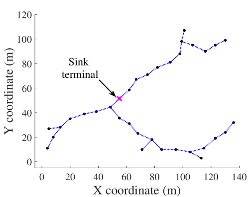
Figure 4: Routing connectivity of a multi-hop, $34$-terminal WSN. Sink terminal is depicted with ’x’ marker. Overall connectivity among WSN terminals depends on radio sensitivity and propagation environment and also includes interference connectivity.

The $34$-terminal multi-hop network of Fig. 4 has relative sparse interference connectivity, since every terminal can hear from $3$ to $8$ transmissions. Routing links offer received SNR values that exceed $-90$ dBm and no retransmissions are allowed. Other parameters are given in Table II and simulation implementation details for the GBCA and MinMax algorithms can be found in [46].

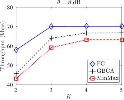
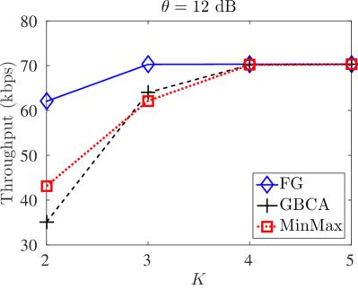
Figure 5: Left (Right): Throughput versus number of frequency channels, for SINR receiver threshold $\theta=8$dB ($\theta=12$dB) and network of Fig. 4.

Fig.  5 illustrates the throughput as a function of available frequency channels ($K$) and receiver SINR threshold $\theta$, for the topology in Fig. 4. The latter is receiver-dependent and controls the number of detected interfering links; higher $\theta$ results to larger number of detected interfering links, better interference reduction and higher computational cost. It can be seen that as the number of available frequency channels increases, higher throughput is achieved for all protocols as expected, since frequency channel availability reduces or eliminates interference. Fig. 5 shows that for all $\theta$ no algorithm achieves $100\%$ packet delivery ratio, or equivalently $87.36$ kbps throughput performance. This stems from the fact that for the specific topology, received SNR in routing tree links was relatively small due to the large distances, compromising reliability and packet delivery ratio.

Interestingly, for $\theta=8$ dB, FG method outperforms the other two algorithms in terms of throughput, for any number of available channels. From Fig. 4 we note that for $K\geq 3$, the throughput of the FG method is not improved significantly and stays almost fixed. It can be seen that for $K=2$, FG offers a throughput gain of $27\%$ compared to GBCA and $34\%$ compared to MinMax. In Fig 5-Right the throughput performance for $\theta=12$ dB is depicted. It is noted that the throughput performance of all algorithms becomes the same for $K\geq 4$ in both cases. For $\theta=12$ dB, the maximum throughput gain of FG over GBCA and MinMax is $76\%$ and $44\%$, respectively. In all examined cases, the maximum packet delivery ratio was approximately $80\%$. The superiority of FG method stems from the fact that frequency and time allocation is jointly applied during the algorithm, offering more degrees of freedom to eliminate the interference. In contrast, the other two algorithms divide the time scheduling and frequency assignment in separate phases during their execution.

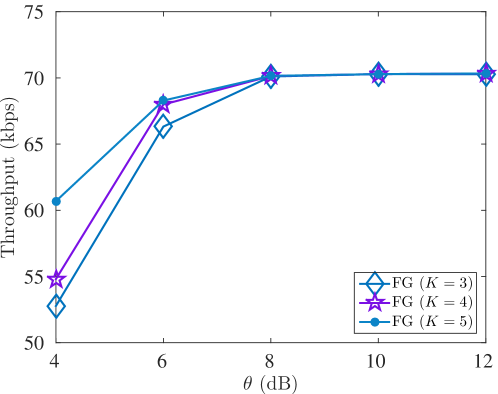
Figure 6: FG throughput versus receiver SINR threshold $\theta$ for different number of frequency channels for network of Fig. 4.

Fig. 6 examines the impact of number of available frequency channels $K$ on throughput performance over different values of threshold $\theta$. It is noted that as the value of SINR parameter $\theta$ increases, throughput is also increased. The proposed algorithm outperforms both GBCA and MinMax in all cases. We include for clarity only the proposed FG algorithm and observe that parameter threshold $\theta=8$ dB is sufficient for the FG algorithm to eliminate interference, offering total throughput of approximately $70$ kbps. This is highly encouraging given that the proposed FG methodology exploited a simplified interference set detection only among terminals with transmissions that can be heard and decoded, as opposed to several smaller received power transmissions which cannot be properly received, but their aggregate sum may be non-negligible. Nevertheless, it is again emphasized that simulations were performed adhering to the natural physics of interference, where whichever WSN terminal transmitted within the same frequency channel and time slot was taken into account in SINR and respective network performance evaluation. Thus, the FG can in principle reduce but not eliminate remaining interference.

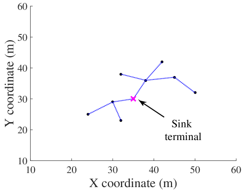
Figure 7: A 3-hop, 9-terminal WSN topology utilized for convergence failure (outage) evaluation.

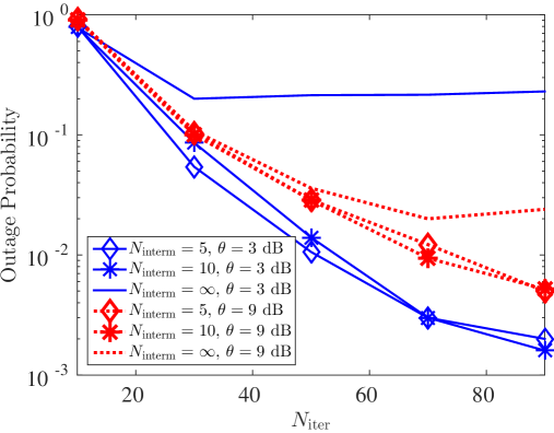
Figure 8: Outage probability of convergence to a valid solution VS maximum number of iterations, $N_{\rm iter}$, for the 9-terminal, 3-hop topology of Fig. 7 and various values of $N_{\rm interm}$.

Finally, the 9-terminal, 3-hop topology of Fig. 7 is considered. In Fig. 8 we plot the outage probability of the proposed FG channel allocation algorithm as a function of $N_{\rm iter}$ for $3$ different values of $N_{\text{interm}}$, using $K=2$ frequency channels and $\theta=3$ dB or $\theta=9$ dB. The results here are obtained by averaging over $5000$ Monte Carlo experiments. The probability of outage is defined as follows:

$$\mathsf{P}_{\rm out}(N_{\rm iter})\triangleq\text{Pr}\!\left(\mathsf{FG}\!\left(\widehat{\mathbf{x}}^{(N_{\rm iter})}\right)=0\right),$$ (28)

i.e., the probability of FG convergence to a non-valid solution after $N_{\rm iter}$ iterations. Fig. 8 demonstrates that, as the number of maximum iterations increase, the proposed modification of loopy BP decreases the probability of outage. It is noted that the proposed modification of loopy BP can offer outage less than $0.002$ for $N_{\rm iter}=90$ with threshold $\theta=3$ dB ($0.005$ for $N_{\rm iter}=90$ with threshold $\theta=9$ dB), in contrast to classical loopy BP, which offers outage probability $0.2$ for $\theta=3$ dB ($0.02$ for $\theta=9$ dB). Thus, we conclude that the proposed modification in loopy BP is in practice necessary for probabilistic distributed channel allocation using the FG framework. This finding is important for network setups with high FG graph degree, either due to large $\theta$ or high WSN terminal density.

VI Conclusion

Factor graph-based, joint time slot/frequency channel allocation is possible in resource-constrained WSNs, even with truly distributed ways, i.e., local message-passing between neighboring WSN terminals, provided that special modifications are introduced for: a) practical detection of interfering terminals and b) convergence of the underlying inference algorithm. The contribution of this work is twofold: this work provides a mathematical framework to show convergence of loopy BP to a valid solution, when such solution exists and the messages can be properly (re-)initialized; it also offers a truly distributed probabilistic algorithm that can be implemented with realistic (even though simplified) practical detection of interferers. Throughput performance of the proposed scheme was evaluated taking into account the true nature of interference, offering promising results. The field of distributed resource allocation has been tremendously challenging and this work has barely scratched the surface, hopefully sparking further interest in the near future towards inference-based methodologies. Modern wireless transmission technologies, e.g., based on full-duplex radio or network coding, could be easily incorporated by proper modifications of the constraints, left for future work.

Appendix A Definition of FG Factor Nodes

The definition of $\mathsf{f,h}$ and $\mathsf{t}$ factors is provided below:
 
function : $\mathsf{f}_{i,m}$
 
Input: $\mathbf{s}_{\mathsf{f}_{i,m}}$
(1): if $\left(\left\|\mathbf{s}_{\mathsf{f}_{i,m}}\right\|_{0}=0~{}~{}{\bf OR}~{}~{}\left\|\mathbf{s}_{\mathsf{f}_{i,m}}\right\|_{0}=1\right)$
(2):     return $1~{}~{}~{}$
(3): else if $\left(\left\|\mathbf{s}_{\mathsf{f}_{i,m}}\right\|_{0}\geq|\mathcal{N}_{\rm TwoH}(i)|\right)$
(4):     return $0$ // constraints 2. or 3.
(5): else
(6):     for$\left\{i_{1}\in\mathcal{N}_{\rm TwoH}(i),k_{1}\in\mathcal{K}:{s}_{i_{1},m}^{(k_{1})}=1\right\}$
(7):     for$\left\{i_{2}\in\mathcal{N}_{\rm TwoH}(i),k_{2}\in\mathcal{K}:{s}_{i_{2},m}^{(k_{2})}=1,[i_{2},k_{2}]\neq[i_{1},k_{1}]\right\}$
(8):        if $\left(k_{1}\neq k_{2}\right)$
(9):           if $\left(i_{1}\in\left\{\left\{\mathcal{N}_{\rm OneH}(i_{2})\cup\mathcal{N}_{\rm sib}(i_{2})\right\}\cap\mathcal{N}_{\rm TwoH}(i)\right\}\right)$
(10):                return $0$ // constraints 1., 2., and 3.
(11):         end if
(12):      else
(13):          if $\left(i_{1}\in\left\{\mathcal{N}_{\rm TwoH}(i_{2})\cap\mathcal{N}_{\rm TwoH}(i)\right\}\right)$
(14):              return $0$ // constraint 4.
(15):          end if
(16):      end if
(17):   end double for
(18):   return $1$
(19): end if
(20): return $0$
 

 
function : $\mathsf{h}_{i,m}$
 
Input: $\mathbf{s}_{\mathsf{h}_{i,m}}$
(1): if $\left(\left\|\mathbf{s}_{\mathsf{h}_{i,m}}\right\|_{0}=0~{}~{}{\bf OR}~{}~{}\left\|\mathbf{s}_{\mathsf{h}_{i,m}}\right\|_{0}=1\right)$
(2):     return $1$
(3): else if $\left(\left\|\mathbf{s}_{\mathsf{h}_{i,m}}\right\|_{0}\geq{\rm min}\{K+1,|\mathcal{I}_{\rm interf}(i)|\}\right)$
(4):     return $0$ // constraints 2. or 3.
(5): else
(6):     for$\left\{i_{1}\in\mathcal{I}_{\rm interf}(i),k_{1}\in\mathcal{K}:{s}_{i_{1},m}^{(k_{1})}=1\right\}$
(7):     for$\left\{i_{2}\in\mathcal{I}_{\rm interf}(i),k_{2}\in\mathcal{K}:{s}_{i_{2},m}^{(k_{2})}=1,[i_{2},k_{2}]\neq[i_{1},k_{1}]\right\}$
(8):       if $(k_{1}=k_{2})$    
(9):          return $0$ // constraint 5.
(10):     end if
(11):     if $(i_{1}=i_{2})$
(12):         return $0$ // constraint 3.
(13):     end if
(14):     if $\left(i_{1}=i\cap i_{2}={\rm par}(i))\right)$
(16):         return $0$ // constraint 2.
(17):     end if
(18):   end double for
(19):   return $1$
(20): end if
(21): return $0$
 

 
function : $\mathsf{t}_{i}$
 
Input: $\mathbf{s}_{\mathsf{t}_{i}}$
(1): if $\left(\left\|\mathbf{s}_{\mathsf{t}_{i}}\right\|_{0}=1\right)$
(2):     return $1$
(3): end if
(4): return $0$
 

Appendix B Proof of Theorem 1

Two auxiliary lemmas are shown first.

Lemma 1.

Under the assumptions of Theorem 1,

$$\mathsf{r}_{v}^{(1)}\!\left(\mathtt{x}_{v}^{\star}\right)>\mathsf{r}_{v}^{(1)}\!\left(1-\mathtt{x}_{v}^{\star}\right),\;\;\forall v\in\mathcal{V},$$ (29)

i.e., the algorithm offers outputs $\widehat{x}^{(1)}_{v}=\mathtt{x}_{v}^{\star},\,\forall v\in\mathcal{V}$.

Proof:

Suppose that prior values $\{q_{v}\}_{v\in\mathcal{V}}$ satisfy Eq. (23). That initialization implies the following:

$$\text{P}_{v}(\mathtt{x}_{v}^{\star})>1-\epsilon_{v}\geq\frac{1}{2}\geq\epsilon_{v}>\text{P}_{v}(1-\mathtt{x}_{v}^{\star}),~{}~{}~{}\forall v\in\mathcal{V}.$$ (30)

During the first iteration, the variable nodes propagate their messages to factor nodes, in order to calculate the outgoing messages. More specifically, $\forall v\in\mathcal{V}$ and $\forall J\in\mathcal{J}_{v}$,

$$\mathsf{m}^{(0)}_{v\rightarrow J}(0)= ~{}q_{v}=\text{P}_{v}(0)$$ (31a)

$$\mathsf{m}^{(0)}_{v\rightarrow J}(1)= ~{}1-\mathsf{m}^{(0)}_{v\rightarrow J}(0)=1-q_{v}=\text{P}_{v}(1).$$ (31b)

An arbitrary variable index $v_{0}\in\mathcal{V}$ is chosen. Due to the fact that factors $\mathsf{g}_{J},J\in\mathcal{J}$ have range {0,1}, the update rule of Eq. (15) can be written, for any $J\in\mathcal{J}_{v_{0}}$, as follows:

$$\mathsf{m}^{(1)}_{J\rightarrow v_{0}}\!\!\left(\mathtt{x}_{v_{0}}^{\star}\right) =\mathtt{C}_{J\rightarrow v_{0}}^{(1)}(\mathbf{q})\!\!\!\!\!\sum_{\begin{smallmatrix}\mathbf{x}_{\mathcal{V}_{J}}:\mathsf{g}_{J}(\mathbf{x}_{\mathcal{V}_{J}})=1\\ x_{v_{0}}=\mathtt{x}_{v_{0}}^{\star}\end{smallmatrix}}\prod_{y\in\mathcal{V}_{J}\backslash v_{0}}\!\!\mathsf{m}^{(0)}_{y\rightarrow J}(x_{y}),$$ (32)

$$\mathsf{m}^{(1)}_{J\rightarrow v_{0}}\!\!\left(1-\mathtt{x}_{v_{0}}^{\star}\right) =\mathtt{C}_{J\rightarrow v_{0}}^{(1)}(\mathbf{q})\!\!\!\!\!\sum_{\begin{smallmatrix}\mathbf{x}_{\mathcal{V}_{J}}:\mathsf{g}_{J}(\mathbf{x}_{\mathcal{V}_{J}})=1\\ x_{v_{0}}=1-\mathtt{x}_{v_{0}}^{\star}\end{smallmatrix}}\prod_{y\in\mathcal{V}_{J}\backslash v_{0}}\!\!\mathsf{m}^{(0)}_{y\rightarrow J}(x_{y}).$$ (33)

It is noted that the summation in Eq. (32) scans all vectors $\mathbf{x}_{\mathcal{V}_{J}}$ with $x_{v_{0}}=\mathtt{x}_{v_{0}}^{\star}$ that satisfy $\mathsf{g}_{J}(\mathbf{x}_{\mathcal{V}_{J}})=1$; it also remarked that the configuration $\boldsymbol{x}_{\mathcal{V}_{J}}^{\star}$ denotes the elements of $\boldsymbol{x}^{\star}$ associated with factor $\mathsf{g}_{J}$ and satisfies $\mathsf{g}_{J}(\mathbf{x}_{\mathcal{V}_{J}}=\boldsymbol{x}_{\mathcal{V}_{J}}^{\star})=1$. Given that Theorem 1 assumes existence of at least one solution, the configuration space of the summation in Eq. (32) contains at least $1$ feasible configuration $\mathbf{x}_{\mathcal{V}_{J}}$ ($\boldsymbol{x}_{\mathcal{V}_{J}}^{\star}$ is one of them). Thus, using the above observation and substituting Eq. (31) in (32), the following inequality is obtained:

$$\mathsf{m}^{(1)}_{J\rightarrow{v_{0}}}\!\!\left(\mathtt{x}_{v_{0}}^{\star}\right) =\mathtt{C}_{J\rightarrow{v_{0}}}^{(1)}(\mathbf{q})\sum_{\begin{smallmatrix}\mathbf{x}_{\mathcal{V}_{J}}:\mathsf{g}_{J}(\mathbf{x}_{\mathcal{V}_{J}})=1\\ x_{v_{0}}=\mathtt{x}_{v_{0}}^{\star}\end{smallmatrix}}\prod_{y\in\mathcal{V}_{J}\backslash v_{0}}\!\!\text{P}_{y}(x_{y})$$

$$\geq\mathtt{C}_{J\rightarrow v_{0}}^{(1)}(\mathbf{q})\!\!\prod_{y\in\mathcal{V}_{J}\backslash v_{0}}\!\!\!\text{P}_{y}\!\left(\mathtt{x}_{y}^{\star}\right).$$ (34)

The marginal of variable $x_{v_{0}}$ for the first iteration is given by Eq. (18) for $n=1$; using Eqs. (30) and (34), the marginal for $x_{v_{0}}=\mathtt{x}_{v_{0}}^{\star}$ is lower bounded:

$$\mathsf{r}_{v_{0}}^{(1)}\!\left(\mathtt{x}_{v_{0}}^{\star}\right) =\text{P}_{v}(\mathtt{x}_{v_{0}}^{\star})\prod_{J\in\mathcal{J}_{v_{0}}}\mathsf{m}^{(1)}_{J\rightarrow v_{0}}(\mathtt{x}_{v_{0}}^{\star})$$

$$\overset{}{>}(1-\epsilon_{v_{0}})\prod_{J\in\mathcal{J}_{v_{0}}}\mathtt{C}_{J\rightarrow v_{0}}^{(1)}(\mathbf{q})\!\!\prod_{y\in\mathcal{V}_{J}\backslash v_{0}}\!\!\!\text{P}_{y}\!\left(\mathtt{x}_{y}^{\star}\right).$$ (35)

An upper bound for $\mathsf{r}_{v_{0}}^{(1)}\!\left(1-\mathtt{x}_{v_{0}}^{\star}\right)$ is found, exploiting Eq. (30), i.e., $\text{P}_{v}\!\left(\mathtt{x}_{v}^{\star}\right)>\frac{1}{2}>\text{P}_{v}\!\left(1-\mathtt{x}_{v}^{\star}\right)$ for any $v\in\mathcal{V}$. For any $J\in\mathcal{J}_{v_{0}}$,

$$\prod_{y\in\mathcal{V}_{J}\backslash v_{0}}\text{P}_{y}(\mathtt{x}_{y}^{\star}) =\max_{\mathbf{x}_{\mathcal{V}_{J}\backslash v_{0}}\in\mathds{B}^{|\mathcal{V}_{J}|-1}}\!\prod_{y\in\mathcal{V}_{J}\backslash v_{0}}\text{P}_{y}(x_{y})$$ (36a)

$$\overset{\eqref{eq:mu_var_to_fac_iter0}}{=}\max_{\mathbf{x}_{\mathcal{V}_{J}\backslash v_{0}}\in\mathds{B}^{|\mathcal{V}_{J}|-1}}\!\!\prod_{y\in\mathcal{V}_{J}\backslash v_{0}}\mathsf{m}^{(0)}_{y\rightarrow J}(x_{y}).$$ (36b)

Using Eq. (31) in (33), applying the definition of $\kappa_{v_{0}}$ and exploiting Eq. (36),

$$\mathsf{m}^{(1)}_{J\rightarrow{v_{0}}}\!\left(1-\mathtt{x}_{v_{0}}^{\star}\right)\! =\mathtt{C}_{J\rightarrow v_{0}}^{(1)}(\mathbf{q})\!\!\sum_{\begin{smallmatrix}\mathbf{x}_{\mathcal{V}_{J}}:\mathsf{g}_{J}(\mathbf{x}_{\mathcal{V}_{J}})=1\\ x_{v_{0}}=1-\mathtt{x}_{v_{0}}^{\star}\end{smallmatrix}}\prod_{y\in\mathcal{V}_{J}\backslash v_{0}}\!\!\text{P}_{y}(x_{y})$$

$$\overset{\eqref{eq:k1}}{\leq}\mathtt{C}_{J\rightarrow v_{0}}^{(1)}(\mathbf{q})~{}\kappa_{v_{0}}\!\!\!\max_{\mathbf{x}_{\mathcal{V}_{J}\backslash v_{0}}\in\mathds{B}^{|\mathcal{V}_{J}|-1}}\!\!\!\prod_{y\in\mathcal{V}_{J}\backslash v_{0}}\!\!\text{P}_{y}(x_{y})$$

$$\overset{\eqref{eq:argmax_x_V_j_A}}{=}\mathtt{C}_{J\rightarrow v_{0}}^{(1)}(\mathbf{q})~{}\kappa_{v_{0}}\prod_{y\in\mathcal{V}_{J}\backslash v_{0}}\text{P}_{y}(\mathtt{x}_{y}^{\star}).$$ (37)

Therefore, the marginal of $v_{0}$ satisfies the following:

$$\mathsf{r}_{v_{0}}^{(1)}\!\left(1-\mathtt{x}_{v_{0}}^{\star}\right) =\text{P}_{v}(1-\mathtt{x}_{v_{0}}^{\star})\prod_{J\in\mathcal{J}_{v_{0}}}\mathsf{m}^{(1)}_{J\rightarrow v_{0}}\!\!\left(1-\mathtt{x}_{v_{0}}^{\star}\right)$$

$$\overset{\eqref{def_prior}}{\underset{\eqref{eq:ineq_mu_J_v_0_iter_1}}{<}}\epsilon_{v_{0}}\prod_{J\in\mathcal{J}_{v_{0}}}\kappa_{v_{0}}~{}\mathtt{C}_{J\rightarrow{v_{0}}}^{(1)}(\mathbf{q})\prod_{y\in\mathcal{V}_{J}\backslash v_{0}}\text{P}_{y}(\mathtt{x}_{y}^{\star})$$

$$\overset{}{=}\epsilon_{v_{0}}~{}(\kappa_{v_{0}})^{\left|\mathcal{J}_{v_{0}}\right|}\!\!\prod_{J\in\mathcal{J}_{v_{0}}}\mathtt{C}_{J\rightarrow{v_{0}}}^{(1)}(\mathbf{q})\!\!\prod_{y\in\mathcal{V}_{J}\backslash v_{0}}\text{P}_{y}(\mathtt{x}_{y}^{\star})$$

$$\overset{(a)}{=}(1-\epsilon_{v_{0}})\prod_{J\in\mathcal{J}_{v_{0}}}\mathtt{C}_{J\rightarrow{v_{0}}}^{(1)}(\mathbf{q})\prod_{y\in\mathcal{V}_{J}\backslash v_{0}}\text{P}_{y}(\mathtt{x}_{y}^{\star})$$

$$\overset{\eqref{marginal_iter_1_for_bit0}}{<}\mathsf{r}_{v_{0}}^{(1)}\!\left(\mathtt{x}_{v_{0}}^{\star}\right),$$ (38)

where step $(a)$ above used that $\epsilon_{v_{0}}\!\left((\kappa_{v_{0}})^{\left|\mathcal{J}_{v_{0}}\right|}+1\right)=1$, stemming directly from the definition of $\epsilon_{v_{0}}$. The choice of $v_{0}\in\mathcal{V}$ and $J\in\mathcal{J}_{v_{0}}$ was arbitrary and thus, the proof is completed. ∎

Lemma 2.

Under the assumptions of Theorem 1,

$$\mathsf{m}^{(1)}_{v\rightarrow J}\!\left(\mathtt{x}_{v}^{\star}\right)>\mathsf{m}^{(1)}_{v\rightarrow J}\!\left(1-\mathtt{x}_{v}^{\star}\right),\forall v\in\mathcal{V},\forall J\in\mathcal{J}_{v}.$$ (39)

Proof:

Suppose that prior values $\{q_{v}\}_{v\in\mathcal{V}}$ satisfy Eq. (23). Consider an arbitrary $v_{0}\in\mathcal{V}$ and $J\in\mathcal{J}_{v_{0}}$. Using the update rule in Eq. (16) and applying the same reasoning with Lemma 1, the following is offered:

$$\frac{\mathsf{m}^{(1)}_{v_{0}\rightarrow J}\!\left(\mathtt{x}_{v_{0}}^{\star}\right)}{\mathtt{C}_{v_{0}\rightarrow J}^{(1)}(\mathbf{q})} =\text{P}_{v_{0}}\!\left(\mathtt{x}_{v_{0}}^{\star}\right)\prod_{I\in\mathcal{J}_{v_{0}}\backslash J}\mathsf{m}^{(1)}_{{I}\rightarrow v_{0}}\!\left(\mathtt{x}_{v_{0}}^{\star}\right)$$

$$\overset{\eqref{def_prior}}{\underset{\eqref{ineq_1}}{>}}(1-\epsilon_{v_{0}})\!\!\prod_{I\in\mathcal{J}_{v_{0}}\backslash J}\!\!\mathtt{C}_{I\rightarrow{v_{0}}}^{(1)}(\mathbf{q})\!\!\!\!\prod_{y\in\mathcal{V}_{I}\backslash v_{0}}\text{P}_{y}(\mathtt{x}_{y}^{\star})$$

$$=\epsilon_{v_{0}}~{}(\kappa_{v_{0}})^{\left|\mathcal{J}_{v_{0}}\right|}\!\!\prod_{I\in\mathcal{J}_{v_{0}}\backslash J}\!\!\mathtt{C}_{I\rightarrow{v_{0}}}^{(1)}(\mathbf{q})\!\!\!\!\prod_{y\in\mathcal{V}_{I}\backslash v_{0}}\text{P}_{y}(\mathtt{x}_{y}^{\star})$$

$$\overset{(a)}{\geq}\!\epsilon_{v_{0}}\!\!\!\prod_{I\in\mathcal{J}_{v_{0}}\backslash J}\!\!\mathtt{C}_{I\rightarrow{v_{0}}}^{(1)}(\mathbf{q})~{}\kappa_{v_{0}}\!\!\!\!\prod_{y\in\mathcal{V}_{I}\backslash v_{0}}\text{P}_{y}(\mathtt{x}_{y}^{\star})$$

$$\overset{\eqref{def_prior}}{\underset{\eqref{eq:ineq_mu_J_v_0_iter_1}}{>}}\!\text{P}_{v_{0}}\!\left(1-\mathtt{x}_{v_{0}}^{\star}\right)\!\!\prod_{I\in\mathcal{J}_{v_{0}}\backslash J}\mathsf{m}^{(1)}_{{I}\rightarrow v_{0}}\!\left(1-\mathtt{x}_{v_{0}}^{\star}\right)$$

$$\overset{}{=}\frac{\mathsf{m}^{(1)}_{v_{0}\rightarrow J}\!\left(1-\mathtt{x}_{v_{0}}^{\star}\right)}{\mathtt{C}_{v_{0}\rightarrow J}^{(1)}(\mathbf{q})},$$ (40)

where step $(a)$ above used that $(\kappa_{v_{0}})^{\left|\mathcal{J}_{v_{0}}\right|}\geq(\kappa_{v_{0}})^{\left|\mathcal{J}_{v_{0}}\right|-1}$, due to the fact that $\kappa_{v_{0}}\geq 1$. The choice of $v_{0}\in\mathcal{V}$ and $J\in\mathcal{J}_{v_{0}}$ was arbitrary and thus, the proof is completed. ∎

Proof:

Suppose that Eq. (23) holds. The theorem will be proved by induction.

Denote for all $n\in\mathds{N}\cup\{0\}$,

$$\mathfrak{T}_{\mathsf{m}}^{(n)}\equiv\prod_{v\in\mathcal{V}}\prod_{J\in\mathcal{J}_{v}}\mathsf{1}\!\left\{\mathsf{m}^{(n)}_{v\rightarrow J}\!\left(\mathtt{x}_{v}^{\star}\right)>\mathsf{m}^{(n)}_{v\rightarrow J}\!\left(1-\mathtt{x}_{v}^{\star}\right)\right\}$$ (41)

and for all $n\in\mathds{N}$,

$$\mathfrak{T}_{\mathsf{r}}^{(n)}\equiv\prod_{v\in\mathcal{V}}\mathsf{1}\!\left\{\mathsf{r}^{(n)}_{v}\!\left(\mathtt{x}_{v}^{\star}\right)>\mathsf{r}^{(n)}_{v}\!\left(1-\mathtt{x}_{v}^{\star}\right)\right\}.$$ (42)

Initialization according to Eq. (23) satisfy Eq. (31), which is equivalent to $\mathfrak{T}_{\mathsf{m}}^{(0)}=1$. Such condition satisfaction offers $\mathfrak{T}_{\mathsf{r}}^{(1)}$ according to Lemma 1 and $\mathfrak{T}_{\mathsf{m}}^{(1)}$ according to Lemma 2. Therefore, the following holds:

$$\mathfrak{T}_{\mathsf{m}}^{(0)}=1\overset{\eqref{priors_vals_sufficiency}}{\underset{}{\implies}}\mathfrak{T}_{\mathsf{r}}^{(1)}=1\text{ and }\mathfrak{T}_{\mathsf{m}}^{(1)}=1.$$ (43)

Subsequent section establishes the following:

$$\mathfrak{T}_{\mathsf{m}}^{(n)}=1\overset{\eqref{priors_vals_sufficiency}}{\underset{}{\implies}}\mathfrak{T}_{\mathsf{r}}^{(n+1)}=1\text{ and }\mathfrak{T}_{\mathsf{m}}^{(n+1)}=1,$$ (44)

implying that Eq. (24) is true.

Assume that the induction hypothesis holds, i.e., $\mathfrak{T}_{\mathsf{m}}^{(n)}=1$. We now show the right-hand side of Eq. (44). Choosing an arbitrary $v_{0}\in\mathcal{V}$, similarly to (34), for any $J\in\mathcal{J}_{v_{0}}$, the message $\mathsf{m}^{(n+1)}_{J\rightarrow{v_{0}}}\!\left(\mathtt{x}_{v_{0}}^{\star}\right)$ can be upper bounded as follows:

$$\mathsf{m}^{(n+1)}_{J\rightarrow{v_{0}}}\!\left(\mathtt{x}_{v_{0}}^{\star}\right)\geq\mathtt{C}_{J\rightarrow v_{0}}^{(n+1)}(\mathbf{q})\!\!\prod_{y\in\mathcal{V}_{J}\backslash v_{0}}\!\mathsf{m}^{(n)}_{y\rightarrow J}\left(\mathtt{x}_{y}^{\star}\right).$$ (45)

Using the induction hypothesis $\mathfrak{T}_{\mathsf{m}}^{(n)}=1$, which implies that $\mathsf{m}^{(n)}_{v\rightarrow J}\!\left(\mathtt{x}_{v}^{\star}\right)>\mathsf{m}^{(n)}_{v\rightarrow J}\!\left(1-\mathtt{x}_{v}^{\star}\right)$, $\forall v\in\mathcal{V},J\in\mathcal{J}_{v}$, under the same reasoning followed in (36b), the following is obtained:

$$\prod_{y\in\mathcal{V}_{J}\backslash v_{0}}\!\mathsf{m}^{(n)}_{y\rightarrow J}(\mathtt{x}_{y}^{\star})=\!\max_{\mathbf{x}_{\mathcal{V}_{J}\backslash v_{0}}\in\mathds{B}^{|\mathcal{V}_{J}|-1}}\!\!\prod_{y\in\mathcal{V}_{J}\backslash v_{0}}\!\mathsf{m}^{(n)}_{y\rightarrow J}(x_{y}).$$ (46)

Hence, working as in Eq. (37) and using Eq. (46), for any $J\in\mathcal{J}_{v_{0}}$, the message $\mathsf{m}^{(n+1)}_{J\rightarrow{v_{0}}}\!\left(1-\mathtt{x}_{v_{0}}^{\star}\right)$ is upper bounded:

$$\mathsf{m}^{(n+1)}_{J\rightarrow{v_{0}}}\left(1-\mathtt{x}_{v_{0}}^{\star}\right)\leq\mathtt{C}_{J\rightarrow v_{0}}^{(n+1)}(\mathbf{q})~{}\kappa_{v_{0}}\!\!\prod_{y\in\mathcal{V}_{J}\backslash v_{0}}\!\mathsf{m}^{(n)}_{y\rightarrow J}\left(\mathtt{x}_{y}^{\star}\right).$$ (47)

Substituting Eqs. (45) and (47) in $\mathsf{r}_{v_{0}}^{(n+1)}\!\left(\mathtt{x}_{v_{0}}^{\star}\right)$ and $\mathsf{r}_{v_{0}}^{(n+1)}\!\left(1-\mathtt{x}_{v_{0}}^{\star}\right)$, respectively, after similar algebra as in Eq. (38), the following is obtained:

$$\frac{\mathsf{r}_{v_{0}}^{(n+1)}\!\left(\mathtt{x}_{v_{0}}^{\star}\right)}{\mathsf{r}_{v_{0}}^{(n+1)}\!\left(1-\mathtt{x}_{v_{0}}^{\star}\right)}\overset{}{>}\frac{1-\epsilon_{v_{0}}}{\epsilon_{v_{0}}}\frac{1}{(\kappa_{v_{0}})^{|\mathcal{J}_{v_{0}}|}}=1.$$ (48)

In a similar vein as above, using the same reasoning as in Eq. (40), the following is obtained:

$$\frac{\mathsf{m}^{(n+1)}_{v_{0}\rightarrow J}\!\left(\mathtt{x}_{v_{0}}^{\star}\right)}{\mathsf{m}^{(n+1)}_{v_{0}\rightarrow J}\!\left(1-\mathtt{x}_{v_{0}}^{\star}\right)}\overset{}{>}\frac{1-\epsilon_{v_{0}}}{\epsilon_{v_{0}}}\frac{1}{(\kappa_{v_{0}})^{\left(|\mathcal{J}_{v_{0}}|-1\right)}}\geq 1.$$ (49)

The choice of $v_{0}\in\mathcal{V}$ and $J\in\mathcal{J}_{v_{0}}$ was arbitrary and thus, the induction step in Eq. (44) is established, proving the theorem. Extension to the damped version can be obtained similarly. ∎

References

- [1] J.-C. Chen, Y.-C. Wang, and J.-T. Chen, “A novel broadcast scheduling strategy using factor graphs and the sum-product algorithm,” IEEE Trans. Wireless Commun., vol. 5, no. 6, pp. 1241–1249, Jun. 2006.
- [2] Y. Wu, J. A. Stankovic, T. He, J. Lu, and S. Lin, “Realistic and efficient multi-channel communications in wireless sensor networks,” in Proc. IEEE INFOCOM, Phoenix, ZA, USA, 2008, pp. 1193–1201.
- [3] J. Chen, Q. Yu, P. Cheng, Y. Sun, Y. Fan, and X. Shen, “Game theoretical approach for channel allocation in wireless sensor and actuator networks,” IEEE Trans. Automat. Contr., vol. 56, no. 10, pp. 2332–2344, Oct. 2011.
- [4] A. Saifullah, Y. Xu, C. Lu, and Y. Chen, “Distributed channel allocation protocols for wireless sensor networks,” IEEE Trans. Parallel Distrib. Syst., vol. 99, pp. 2264–2274, Jul. 2013.
- [5] K. R. Chowdhury, P. Chanda, D. P. Agrawal, and Q. A. Zeng, “DCA - A distributed channel allocation scheme for wireless sensor networks,” in Proc. IEEE PIMRC, Berlin, Germany, Sep. 2005, pp. 1–11.
- [6] G. Zhou, C. Huang, T. Yan, T. He, J. A. Stankovic, and T. F. Abdelzaher, “Mmsn: Multi-frequency media access control for wireless sensor networks,” in Proc. IEEE INFOCOM, Barcelona, Spain, Apr. 2006, pp. 1–13.
- [7] H. K. Le, D. Henriksson, and T. Abdelzaher, “A practical multi-channel media access control protocol for wireless sensor networks,” in Proc. ACM IPSN, St. Louis, Missouri, USA, Apr. 2008, pp. 70–81.
- [8] X. Wang, X. Wang, X. Fu, G. Xing, and N. Jha, “Flow-based real-time communication in multi-channel wireless sensor networks,” in Proc. EWSN, Cork, Ireland, Feb. 2009, pp. 33–52.
- [9] O. Chipara, C. Lu, and J. Stankovic, “Dynamic conflict-free query scheduling for wireless sensor networks,” in Proceedings of the 2006 IEEE International Conference on Network Protocols, Washington, DC, USA, 2006, pp. 321–331.
- [10] G. Zhou, T. He, J. A. Stankovic, and T. Abdelzaher, “RID: Radio interference detection in wireless sensor networks,” in Proc. IEEE INFOCOM, vol. 2, Miami, FL, 2005, pp. 891–901.
- [11] Y. Kim, H. Shin, and H. Cha, “Y-mac: An energy-efficient multi-channel mac protocol for dense wireless sensor networks,” in Proc. ACM IPSN, St. Louis, Missouri, USA, Apr. 2008, pp. 53–63.
- [12] L. Tang, Y. Sun, O. Gurewitz, and D. B. Johnson, “Em-mac: a dynamic multichannel energy-efficient mac protocol for wireless sensor networks,” in Proc. ACM MobiHoc, Paris, France, 2011, pp. 1 –11.
- [13] TelosB. [Online]. Available: http://www.willow.co.uk/TelosB_Datasheet.pdf
- [14] X. Lin and S. B. Rasool, “Distributed and provably efficient algorithms for joint channel-assignment, scheduling, and routing in multichannel ad hoc wireless networks,” IEEE/ACM Trans. Netw., vol. 17, no. 6, pp. 1874–1887, Dec. 2009.
- [15] O. D. Incel, L. van Hoesel, P. Jansen, and P. Havinga, “Mc-lmac: A multi-channel MAC protocol for wireless sensor networks,” Ad Hoc Netw., vol. 9, no. 1, pp. 73–94, Jan. 2011.
- [16] B. Han, V. S. A. Kumar, M. V. Marathe, S. Parthasarathy, and A. Srinivasan, “Distributed strategies for channel allocation and scheduling in software-defined radio networks,” in Proc. IEEE INFOCOM, Rio de Janeiro, Brazil, 2009, pp. 1521–1529.
- [17] R. Vedantham, S. Kakumanu, S. Lakshmanan, and R. Sivakumar, “Component based channel assignment in single radio, multi-channel ad hoc networks,” in Proc. ACM MobiCom, Los Angeles, CA, USA, 2006, pp. 378–389.
- [18] D. P. Bertsekas and J. N. Tsitsiklis, Parallel and Distributed Computation: Numerical Methods. Upper Saddle River, NJ, USA: Prentice-Hall, Inc., 1989.
- [19] Y. Weiss and W. T. Freeman, “On the optimality of solutions of the max-product belief-propagation algorithm in arbitrary graphs,” IEEE Trans. Inf. Theor., vol. 47, no. 2, pp. 736–744, Sep. 2001.
- [20] S. C. Tatikonda and M. I. Jordan, “Loopy belief propagation and gibbs measures,” in Proc. Uncertainty in Artificial Intelligence (UAI), San Francisco, CA, 2002, pp. 493–500.
- [21] T. Heskes, “On the uniqueness of loopy belief propagation fixed points,” Neural Comput., vol. 16, no. 11, pp. 2379–2413, Nov. 2004.
- [22] A. Braunstein, M. Mézard, and R. Zecchina, “Survey propagation: An algorithm for satisfiability,” Random Structures Algorithms, vol. 27, no. 2, pp. 201–226, Mar. 2005.
- [23] A. T. Ihler, J. W. Fischer III, and A. S. Willsky, “Loopy belief propagation: Convergence and effects of message errors,” J. Mach. Learn. Res., vol. 6, pp. 905–936, Dec. 2005.
- [24] J. M. Mooij and H. J. Kappen, “Sufficient conditions for convergence of the sum-product algorithm,” IEEE Trans. Inf. Theory, vol. 53, no. 12, pp. 4422–4437, Dec. 2007.
- [25] M. Bayati, D. Shah, and M. Sharma, “Max-product for maximum weight matching: Convergence, correctness, and LP duality,” IEEE Trans. Inf. Theory, vol. 54, no. 3, pp. 1241–1251, Mar. 2008.
- [26] M. Bayati, C. Borgs, J. Chayes, and R. Zecchina, “On the exactness of the cavity method for weighted b-matchings on arbitrary graphs and its relation to linear programs,” Journal of Statistical Mechanics: Theory and Experiment, vol. 2008, no. 06, Jun. 2008.
- [27] M. Bayati and A. Montanari, “The dynamics of message passing on dense graphs, with applications to compressed sensing,” IEEE Trans. Inf. Theor., vol. 57, no. 2, pp. 764–785, Feb. 2011.
- [28] N. Noorshams and M. J. Wainwright, “Stochastic belief propagation: A low-complexity alternative to the sum-product algorithm,” IEEE Trans. Inf. Theory, vol. 59, no. 4, pp. 1981–2000, Apr. 2013.
- [29] J.-H. Chang and L. Tassiulas, “Energy conserving routing in wireless ad-hoc networks,” in Proc. IEEE INFOCOM, Tel Aviv, Israel, 2000, pp. 22–31.
- [30] P. Andreou, D. Zeinalipour-Yazti, P. K. Chrysanthis, and G. Samaras, “Workload-aware query routing trees in wireless sensor networks,” in Proc. IEEE MDM, Beijing, China, 2008, pp. 189–196.
- [31] A. Deligiannakis, Y. Kotidis, V. Stoumpos, and A. Delis, “Collection trees for event-monitoring queries,” Inf. Syst., vol. 36, no. 2, pp. 386–405, Apr. 2011.
- [32] L. Georgiadis, M. J. Neely, and L. Tassiulas, “Resource allocation and cross-layer control in wireless networks,” Found. Trends Netw., vol. 1, no. 1, pp. 1–144, Apr. 2006.
- [33] Y. Li and A. Ephremides, “A joint scheduling, power control, and routing algorithm for ad hoc wireless networks,” Ad Hoc Networks, vol. 5, no. 7, pp. 959 – 973, Sep. 2007.
- [34] P. N. Alevizos, E. Vlachos, and A. Bletsas, “Factor graph-based distributed frequency allocation in wireless sensor networks,” in Proc. IEEE GLOBECOM, Austin, TX, 2014, pp. 3395–3400.
- [35] D. Gong, M. Zhao, and Y. Yang, “Topology control and channel assignment in lossy wireless sensor networks,” in Proceedings of the 23rd International Teletraffic Congress, San Francisco, California, 2011, pp. 222–229.
- [36] R. G. Gallager, “Low-density parity-check codes,” Ph.D. dissertation, Massachusetts Institute of Technology, 1963.
- [37] T. Richardson and R. Urbanke, Modern Coding Theory. Cambridge University Press, 2008.
- [38] F. R. Kschischang, B. J. Frey, and H.-A. Loeliger, “Factor graphs and the sum-product algorithm,” IEEE Trans. Inf. Theor., vol. 47, pp. 498–519, Feb. 2001.
- [39] H. Loeliger, “An Introduction to factor graphs,” IEEE J. Sel. Topics Signal Process., vol. 21, no. 1, pp. 28–41, Jan. 2004.
- [40] M. R. Shamaiah, S. H. Lee, S. Vishwanath, and H. Vikalo, “Distributed algorithms for spectrum access in cognitive radio relay networks,” IEEE J. Sel. Areas Commun., vol. 30, no. 10, pp. 1947–1957, Nov. 2012.
- [41] S. Rangan, P. Schniter, and A. Fletcher, “On the convergence of approximate message passing with arbitrary matrices,” in Proc. IEEE International Symposium on Information Theory (ISIT), Honolulu, HI, Jun. 2014, pp. 236–240.
- [42] P. N. Stuart Russell, Artificial Intelligence: A Modern Approach, 3rd ed., ser. Prentice Hall Series in Artificial Intelligence. Prentice Hall, 2010.
- [43] J. Flum and M. Grohe, Parameterized Complexity Theory, ser. Texts in Theoretical Computer Science. Springer, 2006.
- [44] A. Boulis, “A simulator for wireless sensor networks and body area networks.” [Online]. Available: http://castalia.npc.nicta.com.au/pdfs/Castalia\%20-\%20User\%20Manual.pdf
- [45] [Online]. Available: http://castalia.npc.nicta.com.au/
- [46] E. A. Vlachos, “Distributed channel allocation algorithms for wireless sensor networks,” Diploma Thesis, School of ECE, Technical University of Crete, Sep. 2012. [Online]. Available: http://users.isc.tuc.gr/~palevizos/euthimis_vlachos_thesis.pdf
- [47] M. Zuniga and B. Krishnamachari, “Analyzing the transitional region in low power wireless links,” in Proc. IEEE SECON ’04, Santa Clara, CA, 2004, pp. 517–526.