Solvo-osmotic flow in electrolytic mixtures

Abstract

We show that an electric field parallel to an electrically neutral surface can generate flow of electrolytic mixtures in small channels. We term this solvo-osmotic flow, since the flow is induced by the asymmetric preferential solvation of ions at the liquid-solid interface. The generated flow is comparable in magnitude to the ubiquitous electro-osmotic flow at charged surfaces, but for a fixed surface charge density, it differs qualitatively in its dependence on ionic strength. Solvo-osmotic flow can also be sensitively controlled with temperature. We derive a modified Helmholtz-Smoluchowski equation that accounts for these effects.

1 Introduction

The use of electric fields to drive flow parallel to charged surfaces at the micro- and nano-scale is ubiquitous in science and technology, with applications in numerous fields, from “Lab-on-a-Chip” devices (Stone et al., 2004; Squires & Quake, 2005) and nanofluidics (Bocquet & Charlaix, 2010) to membrane and soil science, and the separation and analysis of biological macromolecules (Eijkel & Berg, 2005). In its simplest form, the fluid velocity $v_{\infty}$ far from the charged surface is proportional to the applied electric field $E_{0}$, $v_{\infty}=\mu_{e}E_{0}$. The electro-osmotic mobility $\mu_{e}$ is given by the Helmholtz-Smoluchowski equation (von Smoluchowski, 1903), $\mu_{e}=-\varepsilon\zeta/\eta$, where $\varepsilon$ is the solvent permitivity, $\eta$ is the solvent viscosity, and the so-called zeta potential $\zeta$ is the electric potential at the shear plane. In neat (single-component) solvents, this electro-osmotic flow (EOF) has been studied extensively (Delgado et al., 2007), with more recent works focusing on the influence of the channel geometry (Bhattacharyya et al., 2005; Mao et al., 2014), surface slip (Huang et al., 2008; Bouzigues et al., 2008; Maduar et al., 2015; Rankin & Huang, 2016), ion-specificity (Huang et al., 2007) and the solvent rheology (Bautista et al., 2013). EOF in solvent mixtures is common in non-aqueous capillary electrophoresis (Kenndler, 2014), and was investigated also for aqueous mixtures (Valkó et al., 1999; Grob & Steiner, 2002), but the electrokinetics in such systems is not well understood.

The differences between the electrostatics of neat solvents compared to solvent mixtures has also been an area of intense research in recent years, with the growing use of miscible and non-miscible oil-water mixtures in colloidal science and microfluidics. A crucial role is played by the partitioning of ions between solvents, due to their preferential solvation in one of the liquids (Onuki & Kitamura, 2004; Tsori & Leibler, 2007; Zwanikken & van Roij, 2007; Ben-Yaakov et al., 2009; Araki & Onuki, 2009; Samin & Tsori, 2011, 2013; Okamoto & Onuki, 2011; Bier et al., 2011; Pousaneh & Ciach, 2011; Samin & Tsori, 2012; Bier et al., 2012; Pousaneh & Ciach, 2014; Michler et al., 2015; Samin & Tsori, 2016) . The preferential wetting of one liquid at a solid surface or the presence of a liquid-liquid interface therefore also affects the electrostatics of the mixture. It leads to a modification of colloid-colloid (Law et al., 1998; Bonn et al., 2009; Hertlein et al., 2008; Nellen et al., 2011; Samin et al., 2014) as well as colloid-interface interactions (Leunissen et al., 2007a, b; Elbers et al., 2016; Banerjee et al., 2016; Everts et al., 2016). The strength of preferential solvation is measured by the Gibbs transfer energy $k_{B}Tg^{\alpha}$ of an ion species $\alpha$ between two solvents, where $k_{B}T$ is the thermal energy, and $|g^{\alpha}|\sim 1-10$ for aqueous mixtures of relatively polar organic solvents (Kalidas et al., 2000; Marcus, 2007), but can be as large as $15$ in less polar solvents containing antagonistic salts (Onuki et al., 2016). For monovalent salts dissolved in mixtures, the combined effect of both ionic species (Samin & Tsori, 2013; Okamoto & Onuki, 2011; Bier et al., 2011; Michler et al., 2015) is conveniently expressed in terms of the average overall solubility $g_{S}=(g^{+}+g^{-})/2$, and the solubility contrast, $g_{D}=(g^{+}-g^{-})/2$, which for example, determines the Donnan potential $k_{B}Tg_{D}/e$ at oil-water interfaces due to ion partitioning, where $e$ is the elementary charge. In this work, we show that preferential solvation also affects electrokinetic phenomena in mixtures, where it generates an additional, and significant, source of fluid mobility. We find that the dominant contribution to this additional mobility is proportional to $g_{D}$ and is independent of the surface charge, and therefore able to generate flow even at electrically neutral surfaces.

2 Formulation of the problem

Within a continuum theory, we study the flow in a channel containing an electrolytic mixture using direct numerical simulations and a simple linear theory. We consider an oil-water mixture characterized by the order parameter $\varphi$, which is the deviation of the volume fraction of water in the mixture, $\phi$, from its critical value $\phi_{c}$: $\varphi=\phi-\phi_{c}$. The mixture contains point-like monovalent ions with number densities $n^{\pm}$. In our calculations, two cylindrical reservoirs containing the mixture are coaxially connected by a long cylindrical channel with radius $R$, with the $z$ axis being the axis of symmetry and $r$ the radial coordinate. In equilibrium, the composition in both the reservoirs is $\varphi_{0}=0$ and the number densities of ions are $n_{0}$. At the edge of one reservoir, we impose a uniform external electric field $E_{0}\hat{z}$, forcing the charged mixture in the channel, and leading to a flow field $\boldsymbol{v}$.

2.1 Governing equations

To study the mixture dynamics we start from a free energy $F$ of the form

$$\beta F =\int{\rm d}\boldsymbol{{\rm r}}~{}\Bigl{\{}f_{m}(\varphi)+\frac{C}{2}|\bnabla\varphi|^{2}+\frac{\beta}{2}\varepsilon(\varphi)(\bnabla\psi)^{2}$$

$$+\sum_{\alpha=\pm}n^{\alpha}\left[\left(\log(v_{0}n^{\alpha})-1\right)-g^{\alpha}\varphi\right]\Bigr{\}},$$ (1)

where $\beta^{-1}=k_{B}T$ and $v_{0}=a^{3}$ is the molecular volume of both mixture components. The first term in the integrand is the “double-well” bulk mixture free energy density, $v_{0}f_{m}=(\chi-2)\varphi^{2}+4\varphi^{4}/3$, where $\chi\sim 1/T$ is the Flory parameter. This free energy leads to an upper critical solution temperature type phase diagram, with a critical temperature $T_{c}$ and the corresponding critical Flory parameter $\chi_{c}=2$. In this work, we focus on the region $T>T_{c}$ ($\chi<\chi_{c}$), such that the bulk mixture is always homogeneous. The second “square gradient” term accounts for composition inhomogeneities at interfaces, where $C=\chi/a$. The third term is the electrostatic energy density, where $\psi$ is the electric potential, and $\varepsilon(\varphi)$ is the permitivity, assumed to depend linearly on $\varphi$. The final term in the integrand is the ionic free energy, composed of the ideal-gas entropy of ions of species $\alpha=\pm$, and the ionic solvation energy, which is proportional to the Gibbs free energy of transfer $g^{\alpha}$ and local solvent composition. Note that $g^{\alpha}$ can greatly vary between ionic species depending on their size, charge and chemistry.

The relations governing the mixture dynamics read (Araki & Onuki, 2009)

$$\partial\varphi/\partial t+\bnabla\cdot\left(\varphi\boldsymbol{v}\right) =D^{m}\nabla^{2}\beta\mu~{},$$ (2)

$$\partial n^{\alpha}/\partial t+\bnabla\cdot\left(n^{\alpha}\boldsymbol{v}\right) =D^{\alpha}\bnabla\cdot n^{\alpha}\bnabla\beta\lambda^{\alpha},$$ (3)

$$\bnabla\cdot(\varepsilon(\varphi)\bnabla\psi) =-\textstyle\sum_{\alpha}z^{\alpha}n^{\alpha},$$ (4)

$$\bnabla\cdot\boldsymbol{v} =0,$$ (5)

$$\eta\nabla^{2}\boldsymbol{v}-\bnabla p =v_{0}^{-1}\varphi\bnabla\mu+\textstyle\sum_{\alpha}n^{\alpha}\bnabla\lambda^{\alpha}~{}.$$ (6)

equation 2 is the convective Cahn-Hilliard equation, where $D^{m}$ is the inter-diffusion constant of the mixture and $\mu=v_{0}(\delta F/\delta\varphi$) is the solvent chemical potential given by $\beta\mu/v_{0}=-C\nabla^{2}\varphi+f^{\prime}(\varphi)-\beta\varepsilon^{\prime}(\varphi)(\bnabla\psi)^{2}/2-\sum_{\alpha}g^{\alpha}n^{\alpha}$. equations 3 and 4 are the Poisson-Nernst-Planck equations, where $D^{\alpha}$ are ionic diffusion constants and $\lambda^{\alpha}=\delta F/\delta n^{\alpha}$ are the ionic chemical potentials given by $\beta\lambda^{\alpha}=\log(v_{0}n^{\alpha})+\beta z^{\alpha}\psi-g^{\alpha}\varphi$, with $z^{\alpha}=\pm e$. equations 5 and 6 are the Stokes equations at small Reynolds number, where $p$ is the pressure and the right hand side of equation 6 contains the body forces due to concentration gradients.

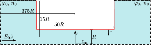
Figure 1: An illustration of the system in the $rOz$ plane. A cylindrical channel with radius $R$ connects two reservoirs containing a salty water–acetonitrile mixture with a composition $\varphi_{0}=0$ and a salt concentration $n_{0}$. The system is driven out of equilibrium by an external electric field $E_{0}$ in the $\hat{z}$ direction. The system dimensions, given in the figure in terms of $R$, ensure that the effect of reservoirs and channel edges on the flow that develops in the channel is small. Different boundary line types indicate different boundary conditions (see text).

An illustration of the computational domain for the numerical solution of equations 2, 3, 4, 5 and 6 is shown in figure 1 (not to scale). Solid walls are indicated by the red lines in figure 1. On these walls, we impose the no-slip boundary condition (BC) for the velocity, $\boldsymbol{v}=0$, and no material fluxes for the composition and ions. The second BC for the composition is $-\boldsymbol{\nu}\cdot\bnabla\varphi=\gamma$, with $\boldsymbol{\nu}$ being the unit normal to the surface. The coefficient $\gamma$ represents the short-range interaction between the solvent mixture and the surface (per solvent molecule). We call $\gamma$ the effective surface field; $\gamma$ is positive (negative) for hydrophilic (hydrophobic) surfaces. The surface may carry a fixed charge density $e\sigma$ which from Gauss’s law implies $-\boldsymbol{\nu}\cdot\bnabla\psi=e\sigma/\varepsilon(\varphi)$.

At the open reservoir edges, indicated by dash-dot lines in figure 1, we set the composition to $\varphi_{0}=0$ and ion densities to $n_{0}$. We also allow the mixture to be freely advected, with vanishing total stress and diffusive fluxes: $-\boldsymbol{\nu}\bcdot\left(p\mathsfbi{1}+\mathsfbi{S}-\mathsfbi{T}\right)=0~{}$, $-\boldsymbol{\nu}\bcdot\bnabla\mu=0$ and $-\boldsymbol{\nu}\bcdot n^{\pm}\bnabla\lambda^{\pm}=0$, respectively, where $\mathsfbi{T}=\eta(\bnabla\boldsymbol{v}+\bnabla\boldsymbol{v}^{T})$ is the viscous stress tensor and $\mathsfbi{S}$ is the total stress tensor given by

$$\beta\mathsfbi{S} =\Bigl{[}\varphi f_{m}^{\prime}(\varphi)-f_{m}-\tfrac{C}{2}|\bnabla\varphi|^{2}-C\varphi\nabla^{2}\varphi-\varphi\varepsilon^{\prime}(\varphi)\frac{\left|\boldsymbol{E}\right|^{2}}{2}+\frac{\boldsymbol{E}\cdot\boldsymbol{D}}{2}$$

$$+\sum_{\alpha=\pm}(1-g^{\alpha}\varphi)n^{\alpha}\Bigr{]}\mathsfbi{1}+C\bnabla\varphi\bnabla\varphi-\boldsymbol{E}\boldsymbol{D}~{},$$ (7)

where $\boldsymbol{E}=-\bnabla\psi$ is the electric field, $\boldsymbol{D}=\varepsilon(\varphi)\boldsymbol{E}$ is the displacement field, and the prime indicts differentiation with respect to the argument. Lastly, the dashed curve in figure 1 is the $r=0$ axis where we apply symmetry BCs for all fields. Numerical simulations in this work were performed using the finite-elements software COMSOL multiphysics.

2.2 Linear theory

To better understand the flow generated in the channel, we first consider a simplified system where we assume that: (i) perturbations in the composition $\varphi-\varphi_{0}$ and ion densities $\delta n^{\pm}=n^{\pm}-n_{0}$ relative to their bulk values are small due to weak adsorption at the channel surface, (ii) the channel is very long such that edge effects are negligible and translational invariance in the $z$ direction applies, (iii) the dominant body force in equation 6 is the electric body force, and (iv) convective composition and ion currents in the channel are negligible since the corresponding Péclet numbers are small. However, even in simple mixtures, transport through channels can lead to complex and surprising effects (Samin & van Roij, 2017), also for small Péclet numbers. Therefore, it is necessary to also solve the complete system equations 2, 3, 4, 5 and 6 numerically to verify that the simplified description is valid.

Within the appropriate parameter regime, the full transport problem can thus be reduced to a steady-state problem, where all fields depend only on $r$. We also decompose the electric potential as $\psi(r,z)=\Psi(r)/(\beta e)-zE_{z}+const$, where $\Psi(r)$ is a dimensionless radial potential and $E_{z}$ is the uniform axial electric field in the channel. Note that $E_{z}\neq E_{0}$ in general. For a fully developed flow, we assume $v_{r}=0$ and thus $v_{z}=v_{z}(r)$ from equation 5. Lastly, we set $\bnabla p=0$ as we focus on the effect of $E_{z}$. Linearizing the simplified equations 2, 3, 4, 5 and 6 (Okamoto & Onuki, 2011; Samin & Tsori, 2013) we find $\delta n^{\pm}=n_{0}(g^{\pm}\varphi\mp\Psi)$ and obtain the system:

$$\xi^{2}\nabla_{r}^{2}\varphi =\varphi+2n_{0}g_{D}(\Psi-g_{D}\varphi)/\tau~{},$$ (8)

$$\lambda_{D}^{2}\nabla_{r}^{2}\Psi =\Psi-g_{D}\varphi~{},$$ (9)

$$\lambda_{D}^{2}\eta\nabla_{r}^{2}v_{z} =\bar{\varepsilon}(\Psi-g_{D}\varphi)E_{z}/(\beta e)~{},$$ (10)

where $\xi=(C/\tau)^{1/2}$ is the modified correlation length and $\tau=2(2-\chi)/v_{0}-2n_{0}g_{S}^{2}$. The Debye length is $\lambda_{D}=(8\pi l_{B}n_{0})^{-1/2}$, where $l_{B}=e^{2}/(4\pi\bar{\varepsilon}k_{B}T)$ is the Bjerrum length with the average permitivity $\bar{\varepsilon}=\varepsilon(\varphi_{0})$.

3 Results

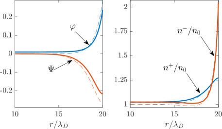
Figure 2: (a) Composition $\varphi(r)$ and scaled potential $\Psi(r)$ at the channel center ($z=0$) and (b) the corresponding scaled cation and anion profiles, for a water–acetonitrile (Sazonov et al., 2007; Wohlfarth, 2009) with a Debye length $\lambda_{D}=1.16$ nm and a correlation length $\xi=1.31$ nm. Solid lines: numerical solution, dashed curves: linear theory (see text). We plot the profiles near the channel surface, where here and in all other figures the channel radius is $R=20\lambda_{D}$. The channel surface is uncharged ($\sigma=0$) and hydrophilic, $\gamma=0.2C$, corresponding to a tension of $\approx 7$ mN/m. The mixture with $\bar{\varepsilon}=58$ and at a temperature of $293$ K ($\chi=1.86$) contains $50$ mM of NaCl ($g^{+}=0,g^{-}=4$). For the mixture properties we use the critical temperature $T_{c}=272$ K, a molecular length $a=3.6$ Å, estimated from a critical density of 900 kg/m³, and a viscosity of $0.7$ mPa s (Sazonov et al., 2007; Wohlfarth, 2009). The liquid permeability is given by $\varepsilon(\varphi)/\varepsilon_{0}=\varepsilon_{\rm acetonitrile}/2+\varepsilon_{\rm water}/2+\left(\varepsilon_{\rm water}-\varepsilon_{\rm acetonitrile}\right)\varphi$, where $\varepsilon_{0}$ is the vacuum permitivity, and we used $\varepsilon_{\rm acetonitrile}=36.6$ and $\varepsilon_{\rm water}=79.5$.

In a cylindrical domain, the profiles $\varphi(r)$ and $\Psi(r)$ of equations 8 and 9 are the linear combinations

$$\Psi(r) =a_{1}\mathrm{I}_{0}(q_{1}r)-a_{2}\mathrm{I}_{0}(q_{2}r)~{},$$ (11)

$$\varphi(r) =b_{1}\mathrm{I}_{0}(q_{1}r)-b_{2}\mathrm{I}_{0}(q_{2}r)~{},$$ (12)

where $\mathrm{I}_{n}$ is the modified Bessel function of the first kind of order $n$, such that the wave numbers $q_{i}$ ($i=1,2$) obey the biquadratic equation

$$\lambda_{D}^{2}q_{i}^{4}-\left[1+(\lambda_{D}/\xi)^{2}-g_{D}^{2}/(4\pi l_{B}C)\right]q_{i}^{2}+\xi^{-2}=0~{}.$$ (13)

The amplitudes $a_{i}$ and $b_{i}$ follow from symmetry at $r=0$ and the BCs given above at the channel surface $r=R$. Making also use of the identity $((q_{1}\lambda_{D})^{2}-1)((q_{2}\lambda_{D})^{2}-1)=g_{D}^{2}/(4\pi l_{B}C)$, which follows from equation 13, the amplitudes read:

$$a_{i}= \frac{g_{D}}{1-(\lambda_{D}q_{i})^{2}}b_{i}~{},$$ (14)

$$b_{i}= \frac{\gamma\left[1-(\lambda_{D}q_{i})^{2}\right]-g_{D}\sigma/C}{\lambda_{D}^{2}q_{i}(q_{2}^{2}-q_{1}^{2})\mathrm{I}_{1}(q_{i}R)}~{}.$$ (15)

We plot in figure 2a the resulting composition and potential profiles for a water–acetonitrile mixture with $n_{0}=50$ mM of NaCl ($\lambda_{D}=1.16$ nm, $g^{+}\approx 0$ and $g^{-}\approx 4$ (Kalidas et al., 2000; Marcus, 2007)) at room temperature ($\chi=1.86$, $\xi=1.31$ nm) inside a channel with radius $R=20\lambda_{D}$. The mixture physical properties are given in the caption of figure 2. We assume that these properties are independent of temperature, except for the mixture inter-diffusion constant $D^{m}$, which follows from $D^{m}=(6\beta\pi\eta\xi)^{-1}$ (Kawasaki, 1970). The ionic diffusion constants are taken to be $D^{\pm}=1\times 10^{-9}$ m²/s.

The channel surface is uncharged ($\sigma=0$), but is hydrophilic ($\gamma=0.2C>0$), resulting in the adsorption of water near the wall. Since the anions are hydrophilic the water “drags” them along, and hence the anions also effectively adsorb at the surface, see the ionic profiles in figure 2b. Although the cations are indifferent to the local composition, they also adsorb at the surface due to electrostatics, but are distributed more broadly. The result is an electric double layer at an uncharged surface (Samin & Tsori, 2013; Samin et al., 2014), even though this layer is overall charge neutral. figure 2 shows a good agreement between the full numerical solutions and the linear theory. The numerical profiles of $\varphi$ and $n^{\pm}$ decay to values that slightly differ from their bulk values due to a weak nonlinear effect induced by solvation (Samin & Tsori, 2016). The thickness of the charged layer at the surface $\rho(r)=2en_{0}(g_{D}\varphi-\Psi)$ could be estimated in experiments from the characteristic lengths $q_{i}^{-1}$. These length scales are to be estimated from equation 13 given data for $\lambda_{D}$, $\xi$ and $g_{D}$.

Although the fluid is overall neutral, the negative ions layer is more strongly adsorbed at the wall. When an external axial electric field is applied, this layer then serves as an effective surface charge, and the adjacent positively charged layer as an effective electric double layer. The result is an induced fluid flow, similar to EOF. The steady-state axial flow profile $v_{z}(r)$ is obtained by putting equations 11 and 12 into equation 10, and imposing the no-slip BC at $r=R$ and symmetry at $r=0$,

$$v_{z}(r)=\frac{\bar{\varepsilon}E_{z}}{\beta e\eta}\sum_{i=1,2}\left(g_{D}b_{i}-a_{i}\right)\frac{\mathrm{I}_{0}(q_{i}r)-\mathrm{I}_{0}(q_{i}R)}{(-1)^{i}(\lambda_{D}q_{i})^{2}}~{},$$ (16)

which for the parameters of figure 2 is plotted in figure 3 (labeled with $\sigma=0$), showing reasonable agreement between the numerical solution and equation 16. Indeed, a flow is generated by the overall neutral but locally charged layer of fluid near the wall. Figure 3 shows that $v_{z}(r)$ quickly saturates to a plug-like flow of a few mm/s. We term this solvation-induced phenomenon solvo-osmotic flow (SOF). This flow is similar and comparable in magnitude to simple EOF, shown in figure 3 by the curve for a neat solvent with the same properties as the mixture, but near a weakly charged surface with $\sigma=-0.012$ nm^-2.

SOF can either combine or work against EOF, as shown by two curves in figure 3, where we used the parameter of figure 2, but with non-zero surface charges, $\sigma=\pm 0.012$ nm^-2. For $\sigma<0$ the result is an enhanced flow with the velocity at the channel center slightly smaller than the sum of SOF and EOF on their own. In a neat solvent, when $\sigma$ changes sign one expects a simple change of sign also for the velocity. However, here SOF opposes EOF for $\sigma>0$ and, for the parameters of figure 3, the result is that inside most of the channel $v_{z}$ remains positive, but with a much smaller magnitude. There is, however, a weak back flow close to the channel wall resulting from the radial component of the body force in the fluid becoming significant in this case.

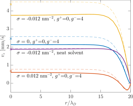
Figure 3: Axial velocity profiles $v_{z}(r)$ at an applied field of $E_{0}=2.5$ V/mm for several scenarios, see the labels in the figure. All other parameters are the same as in figure 2. Numerical results (solid curves) are in good agreement with linear theory (dashed curves), where in equation 16 we used $E_{z}$ from the numerical calculation. Crosses were calculated using equation 18.

In the large-$R$ limit where $R\gg\lambda_{D},\xi$, the fluid moves as a plug, $v_{z}=const.$, and one defines the electro-osmotic mobility of the fluid as $\mu_{e}=v_{z}/E_{z}$. In this limit we find:

$$\mu_{e}=-\frac{\bar{\varepsilon}}{\eta}\frac{4\pi l_{B}\sigma(q_{1}^{2}+q_{2}^{2}+q_{1}q_{2}-\lambda_{D}^{-2})+g_{D}\gamma\lambda_{D}^{-2}}{q_{1}q_{2}(q_{1}+q_{2})\beta e}~{}.$$ (17)

Noting that the biquadratic equation 13 also implies $q_{1}q_{2}=(\xi\lambda_{D})^{-1}$ and $q_{1}^{2}+q_{2}^{2}=\xi^{-2}+\lambda_{D}^{-2}\left[1-g_{D}^{2}/(4\pi l_{B}C)\right]$, and assuming that also $\lambda_{D}/\xi\gg|g_{D}|/(4\pi l_{B}C)$, equation 17 reduces to the modified Helmholtz-Smoluchowski equation

$$\mu_{e}=-\frac{\bar{\varepsilon}}{\eta}\left[\left(4\pi l_{B}\lambda_{D}\sigma+\frac{g_{D}\gamma\xi}{1+\lambda_{D}/\xi}\right)\frac{1}{\beta e}\right]~{}.$$ (18)

Equation 18 is the main result of this paper, where the term in brackets is the zeta potential $\zeta$, with the shear plane located at $r=R$. Only the first term $\propto\sigma$ in equation 18 exists for a neat solvent (Keh & Tseng, 2001). In a mixture, $\zeta$ is determined also by the properties of the salt and surface through the second term $\propto g_{D}\gamma$ in equation 18, which plays the role of an effective surface charge. The attractive feature of equation 18 is the ability to easily tune the fluid mobility through $g_{D}$ without making any surface modification. For example, by replacing the anion Cl^- with the hydrophobic anion BPh${}_{4}^{-}$, we have $g_{D}\approx 6$ (Marcus, 2007) (instead of $g_{D}=-2$), which would then change $\mu_{e}$ drastically, in some cases even its sign. As we show below, the dependence of $\mu_{e}$ on $\xi$ in mixtures opens the possibility to tune the mobility also with temperature, since $\xi$ diverges near the mixture critical temperature. Nevertheless, we stress that $\xi\sim a$ for completely miscible mixtures (the $\chi\rightarrow 0$ limit in our theory). Hence, equation 18 should be applicable to mixtures in general, and as the crosses in figure 3 confirm, it is in good agreement with the numerical results for $v_{z}(0)$.

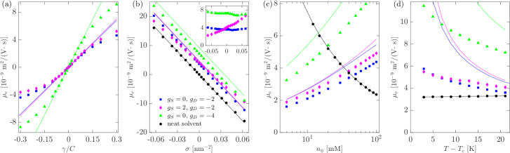
Figure 4: Dependence of fluid mobility $\mu_{e}$ on (a) the surface-solvent coupling $\gamma$, (b) the surface charge $e\sigma$, (c) the salt concentration $n_{0}$ and (d) the temperature $T$, for three types of electrolytic mixtures (see text). Symbols correspond to numerical results and lines to equation 18. In (b)-(d), we plot also $\mu_{e}$ for a neat solvent with the same physical properties as the mixtures (circles). In panels (a)-(c), $T=293$ K is fixed while in panels (a), (b) and (d) we keep $n_{0}=50$ mM fixed. For the mixture data sets in (b)-(d) we took $\gamma=0.2C$ and in (a), (c) and (d) we took $\sigma=0$. For the neat solvent in (c)-(d), we used $\sigma=0.012$ nm^-2. Inset of (b): the shift in mobility between the mixtures and the neat solvent.

In figure 4 we show the effects of varying some of the free parameters of our model on the fluid mobility, and compare numerical results (symbols) with equation 18 (lines). We compare three types of electrolytic mixtures, one containing NaCl (diamonds) as before and two containing so-called antagonistic salts in which one of the ions is hydrophilic and the other hydrophobic. In order to single out the role of $g_{D}$, we choose $g_{S}=0$ by setting $g^{-}=-g^{+}$=2 (squares) and 4 (triangles). figure 4a shows the pure SOF mobility as a function of the surface field $\gamma$, revealing that the linear theory becomes an excellent approximation for small enough $|\gamma|$, for which $\varphi\ll 1$ holds, and that $\mu_{e}$ increases with $\gamma$ and $g_{D}$, as expected from equation 18. Notice that the sign of $\mu_{e}$ depends on the wetting properties of the surface. For the salts having the same solubility contrast $g_{D}$ but different overall solubility $g_{S}$ (squares and diamonds), we find significant differences in the mobility only for large enough $|\gamma|$. In this regime, the ions’ entropy decrease near the wall hinders their adsorption, leading to a reduced mobility compared to the linear theory.

In figure 4b-d we also contrast the electrolytic mixtures with a neat solvent (circles) having the same physical properties as the mixtures. In figure 4b we examine the effect of adding a fixed surface charge $\sigma$. Clearly, here SOF increases the mobility compared to regular EOF in a neat solvent. The inset of figure 4b shows that the shift in mobility is almost constant and increases with $g_{D}$ for the antagonistic salts, as expected from equation 18. The mobility shift is not constant for NaCl, rather it increases with $\sigma$, and the result is an an asymmetry in the mobility when $\sigma$ changes sign, an effect that is absent in neat solvents. This effect originates from the nonlinear coupling between electrostatics and solvation (Samin & Tsori, 2012), and is expressed by the next order term $\propto g_{S}\varphi\Psi$ in the expansion of $\delta n^{\pm}$. This contribution vanishes for our ideal antagonistic salts, but should be relevant for the majority of realistic salts. The relative shift in mobility due to SOF is significant for the weakly to moderately charged surfaces we considered here, which is a common situation for hydrophobic surfaces (Jing & Bhushan, 2013), or in hydrophilic surfaces near their iso-electric point. For the typically highly charged hydrophilic surfaces the contribution of SOF may be small, although this may not always be the case since both $g_{D}$ and $\gamma$ can be much larger than the values used in this work.

In figure 4c-d we show the influence of the salt concentration and temperature, respectively, on mobility. In both panels we compare electrolytic mixtures in an uncharged channel with a neat solvent in a channel with $\sigma=0.012$ nm^-2. Strikingly, figure 4c shows that the mobility increases with $n_{0}$ for the mixtures, while it decreases for the neat solvent. This behaviour follows from the dependence of $\mu_{e}$ on $\lambda_{D}\propto n_{0}^{-1/2}$ in equation 18. For constant $\sigma$, the contribution to the surface potential from the first term in equation 18 becomes smaller when $\lambda_{D}$ decreases, while the second term becomes larger. Figure 4c suggests that for $n_{0}\sim 100$ mM, the contribution to the mobility from solvation could be dominant when the surface is weakly charged. SOF is enhanced by increasing the ionic strength since this leads also to increased ion adsorption at the wall, which results in a larger effective surface charge. The opposite dependence on $n_{0}$ between the two terms in equation 18 can therefore lead to a minimum in the mobility of mixtures at charged surfaces, which is confirmed by numerical calculations (not shown).

Figure 4d demonstrates that, in mixtures, temperature can be used to effectively tune the mobility, whereas its effect is much smaller in neat solvents. The reason is that the correlation length $\xi$ diverges as the $T_{c}$ is approached from the one-phase region at the critical composition. In equation 18, the mobility increases with $\xi$, or equivalently, when the temperature is lowered towards $T_{c}$, which is confirmed by the numerical results in figure 4d. Here, the agreement with the linear theory is not as good since $\varphi$ is no longer small when $T_{c}$ is approached. The numerical results show that $\mu_{e}$ changes by as much at $60\%$ in a temperature window of $20$ K, whereas it essentially remains constant for the neat solvent. We did not account, however, for the change of $\varepsilon$ with temperature. This effect will be at play for both mixtures and neat solvents, and should be smaller since, for example, the permitivity of water changes only by about $10\%$ in the same temperature window.

4 Conclusions

In conclusion, we have shown that the electro-osmotic mobility of mixtures contains an additional contribution due to the preferential solvation of ions. This contribution allows to drive flow at an electrically neutral surface and to vary the mobility significantly by changing the type of salt or the temperature. All of our results can be directly extended to the phoretic motion of particles in an applied field.

A comparison of our results with existing experiments (Valkó et al., 1999; Grob & Steiner, 2002) is difficult to preform at this point, because capillary electrophoresis experiments employ fused silica surfaces, which are typically highly-charged and, more importantly, charge-regulating. A modification of the theory is thus required to better mimic experimental conditions. This should include the chemical dissociation equilibrium at the channel surface, and the change in the fluid viscosity with composition. For the study of transient SOF, one should also consider the asymmetry in the cation and anion diffusion constants, and their dependence on the solvent composition. Our work points towards promising possibilities for the utilization of SOF in the transport of fluids through channels and of colloids by external fields, and we hope it will lead to systematic experiments on the electrokinetics of solvent mixtures.