Variational inference for probabilistic Poisson PCA

Abstract

Many application domains such as ecology or genomics have to deal with multivariate non Gaussian observations. A typical example is the joint observation of the respective abundances of a set of species in a series of sites, aiming to understand the co-variations between these species. The Gaussian setting provides a canonical way to model such dependencies, but does not apply in general. We consider here the multivariate exponential family framework for which we introduce a generic model with multivariate Gaussian latent variables. We show that approximate maximum likelihood inference can be achieved via a variational algorithm for which gradient descent easily applies. We show that this setting enables us to account for covariates and offsets. We then focus on the case of the Poisson-lognormal model in the context of community ecology. We demonstrate the efficiency of our algorithm on microbial ecology datasets. We illustrate the importance of accounting for the effects of covariates to better understand interactions between species.

arXiv:1703.06633

, and

label=e1]julien.chiquet@inra.fr label=e2]mahendra.mariadassou@inra.fr label=e3]robin@agroparistech.fr

1 Introduction

Principal component analysis (PCA) is among the oldest and most popular tool for multivariate analysis. It basically aims at reducing the dimension of a large data set made of continuous variables (Anderson, 2003; Mardia et al., 1979) in order to ease its interpretation and visualization. The methodology exploits the dependency structure between the variables to exhibit the few synthetic variables that best summarize the information content of the whole data set: the principal components. In that sense, PCA can be viewed as a way to better understand the dependency structure between the variables. From a purely algebraic point-of-view, PCA can be seen as a matrix-factorization problem where the data matrix is decomposed as the product of a loading matrix and a score matrix (Eckart and Young, 1936).

For statistical purposes, PCA can also be cast in a probabilistic framework. Probabilistic PCA (pPCA) is a model-based version of PCA originally defined in a Gaussian setting, in which the scores are treated as random hidden variables (Tipping and Bishop, 1999; Minka, 2000). It is closely related to factor analysis. As it involves hidden variables, maximum-likelihood estimates (MLE) can be obtained via an EM algorithm (Dempster et al., 1977). One major interest of the probabilistic approach is that it allows to combine dimension reduction with other modeling tools, such as regression on some available covariates. Because observed variables can be affected by the variations of such covariates, the correction for their potential effects is desirable to avoid the presence of spurious correlations between the responses.

The Gaussian setting is obviously convenient as the dependency structure is entirely encoded in the covariance matrix but pPCA has been extended to more general settings. Indeed, in many applications (Royle and Wikle, 2005; Srivastava and Chen, 2010), Gaussian models need to be adapted to handle specific measurement types, such as binary or count data. For count data, the multivariate Poisson distribution seems a natural counterpart of the multivariate normal. However, no canonical form exist for this distribution (Johnson et al., 1997), and several alternatives have been proposed in the literature including Gamma-Poisson (Nelson, 1985) and lognormal-Poisson (Aitchison and Ho, 1989; Izsák, 2008). The latter takes advantage of the properties of the Gaussian distribution to display a larger panel of dependency structure than the former, but maximum likelihood-based inference raises some issues as the MLE of the covariance matrix is not always positive definite.

A series of works have contributed to extend PCA to a broader class of distributions, typically in the exponential family. The matrix factorization point-of-view has been adopted to satisfy a positivity constraint of the parameters (Lafond, 2015) and to minimize the Poisson loss function (Cao and Xie, 2015) or more general losses (Lee and Seung, 2001) consistent with exponential family noise. Sparse extensions have also been proposed (Witten et al., 2009; Liu et al., 2016). In a model-based context, Collins et al. (2001) suggest to minimize a Bregman divergence to get estimates of the scores: the divergence is chosen according to the distribution at hand and a generic alternating minimization scheme is proposed. Salmon et al. (2014) consider a similar framework and use matrix factorization for the minimization of Bregman divergence. In both cases, the scores are considered as fixed parameters. Mohamed et al. (2009) cast the same model in a Bayesian context and use Monte-Carlo sampling for the inference. Acharya et al. (2015) consider Bayesian inference of the Gamma-Poisson distribution. A Bayesian version of PCA (where both loadings and scores are treated as random) is considered in Li and Tao (2010).

Landgraf (2015) reframes exponential family PCA as an optimization problem with some rank constraints and develops both a convex relaxation and a maximization-minimization algorithm for binomial and Poisson families. Finally Zhou et al. (2012) and Zhou (2016) consider factor analysis in the more complex setting of negative-binomial families. Our approach differs from the previous ones as we only consider scores as random variables, whereas we consider the loadings as fixed parameters, in the exact analog of Tipping and Bishop’s pPCA.

As recalled above, in pPCA, the scores are treated as hidden variables. One of the main issue of non-Gaussian pPCA arises from the fact that their conditional distribution given the observed data is often intractable, which hampers the use of an Expectation-Minimization (EM) strategy. Variational approximations (Jaakkola and Jordan, 2000; Wainwright and Jordan, 2008) have become a standard tool to approximate such conditional distributions. Karlis (2005) uses such an approximation for the inference of the one-dimensional Poisson-lognormal model and derives a variational EM (VEM) algorithm. Hall et al. (2011) provide a theoretical analysis of this approximation for the same model and prove the consistency of the estimators. Indeed, even the conditional distribution of one single hidden coordinate (given all others) is unknown, which makes regular Gibbs sampling inaccessible. As a consequence, Lee and Seung (2001) use moment estimates, whereas, in a Bayesian context, Li and Tao (2010) resort to a variational approximation of the conditional distribution.

Our contribution

We define a general framework for pPCA in the simple exponential family. The model we consider combines dimension reduction (via pPCA) and regression, in order to account for known effects and focus on the remaining dependency structure. Scores are assumed to be Gaussian to allow a large panel of dependency structures. We put a special emphasis on the analysis of count data. We adopt a frequentist setting rather than a Bayesian approach to avoid non-scalable, computing-heavy Monte-Carlo sampling. We use a variational approximation of the conditional distribution of the scores given the observed data to derive a variational lower bound of the likelihood. Since only the scores are assumed to be random, we can prove that this bound is biconcave, i.e. concave in the model parameters and in the variational parameters but not jointly concave in general. Biconcavity allows us to design a gradient-based method rather than a (variational) EM algorithm, traditionally used in this setting.

We illustrate the interest of our model on two examples of microbial ecology. We show that the proposed algorithm is efficient for large datasets such as these encountered in metagenomics. We also show the importance of accounting for covariates and offset, in order to go beyond first-order effects. More specifically, we show how the proposed modeling allows us to distinguish between correlations that are caused by known covariates from those corresponding to an unknown structure and requiring further investigations.

The paper is organized as follows: in Section 2 we introduce pPCA for the exponential family and the variational framework that we consider. Section 3 generalizes the model in the manner of a generalized linear model, in order to handle covariates and offsets. Then, Section 4 is dedicated to the inference and optimization strategy. Section 5 details the special Poisson case and Section 6 devises the visualization, an important issue for non-Gaussian PCA methods. Finally, Section 7 considers applications to two examples from metagenomics: the impact of a pathogenic fungi on microbial communities from tree leaves, and the impact of weaning on piglets gut microbiota.

2 A variational framework for probabilistic PCA in the exponential family

We start this section by stating the probabilistic framework associated to Gaussian probabilistic PCA. Then we show how it can be naturally extended to other exponential families. We finally derive variational lower bounds for the likelihood of pPCA and its gradient, which are the building blocks of our inference strategy.

2.1 Gaussian probabilistic PCA (pPCA)

The probabilistic version of principal component analysis – or pPCA – (Minka, 2000; Mohamed et al., 2009; Tipping and Bishop, 1999) relates a sample of $p$-dimensional observation vectors $\boldsymbol{Y}_{i}$ to a sample of $q$-dimensional vectors of latent variables $\boldsymbol{W}_{i}$ in the following way:

$$\boldsymbol{Y}_{i}=\boldsymbol{\mu}+\boldsymbol{B}\boldsymbol{W}_{i}+\boldsymbol{\varepsilon}_{i},\qquad\boldsymbol{\varepsilon}_{i}\sim\mathcal{N}(\boldsymbol{0}_{p},\sigma^{2}\boldsymbol{I}_{p}).$$ (1)

The parameter $\boldsymbol{\mu}$ allows the model to have main effects. The $p\times q$ matrix $\boldsymbol{B}$ captures the dependence between latent and observed variables. Furthermore, the latent vectors are conventionally assumed to have independent Gaussian components with unit variance, that is to say, $\boldsymbol{W}_{i}\sim\mathcal{N}(\boldsymbol{0}_{q},\boldsymbol{I}_{q})$. This ensures that there is no structure in the latent space. Model (1) can thus be restated as $\boldsymbol{Y}_{i}\sim\mathcal{N}(\boldsymbol{\mu},\boldsymbol{B}\boldsymbol{B}^{\intercal}+\sigma^{2}\boldsymbol{I}_{p})$.

In the following, we consider an alternative formulation stated in a hierarchical framework. Despite its seemingly more complex nature, it lends itself nicely to generalizations. Formally,

$$\begin{array}[]{rll}\text{latent space}&(\boldsymbol{W}_{i})_{i=1,\dots,n}\quad\text{i.i.d.},&\boldsymbol{W}_{i}\sim\mathcal{N}(\boldsymbol{0}_{q},\boldsymbol{I}_{q})\\[4.30554pt] \text{parameter space}&\boldsymbol{Z}_{i}=\boldsymbol{\mu}+\boldsymbol{B}\boldsymbol{W}_{i},&\\[4.30554pt] \text{observation space}&\left(Y_{ij}|Z_{ij}\right)_{i=1,\dots,n;\;j=1,\dots,p}\quad\text{indep.},&Y_{ij}|Z_{ij}\sim\mathcal{N}(Z_{ij},\sigma^{2})\end{array}$$ (2)

In Equation (2), $\boldsymbol{Z}_{i}$ is a linear transform of $\boldsymbol{W}_{i}$ and the last layer $\boldsymbol{Y}_{i}|\boldsymbol{Z}_{i}$ simply corresponds to observation noise. Informally, the latent variables $\boldsymbol{W}_{i}$ (in $\mathbb{R}^{q}$) are mapped to a linear subspace of the parameter space $\mathbb{R}^{p}$ via the $\boldsymbol{Z}_{i}$ which are then pushed into the observation space using Gaussian emission laws. The main idea of this paper is to replace Gaussian emission laws with univariate natural exponential families.

Note that the diagonal nature of the covariance matrix of $\boldsymbol{\varepsilon}_{i}$ specified in (1) now means that, conditionally on $\boldsymbol{Z}_{i}$, all components of $\boldsymbol{Y}_{i}$ are independent. This is why we may consider univariate variables $Y_{ij}|Z_{ij}$ in Formulation (2). Although the observation noises are conditionally independent, the coordinates of a given $\boldsymbol{Y}_{i}$ are not, which makes the model genuinely multivariate. This is further emphasized in Section 5.1.

The loading matrix $\boldsymbol{B}$ is a convenience parameter that is useful for both optimization and visualization of the model but not identifiable per se. Indeed any orthogonal transformation of $\boldsymbol{B}$ leads to the same model: denoting $\boldsymbol{\Sigma}=\boldsymbol{B}\boldsymbol{B}^{\intercal}$, Model (2) can be rephrased as

$$\begin{split}(\boldsymbol{Z}_{i})_{i=1,\dots,n}\,\text{i.i.d.},\,\boldsymbol{Z}_{i}\sim\mathcal{N}(\boldsymbol{\mu},\boldsymbol{\Sigma}),\\ \left(Y_{ij}|Z_{ij}\right)_{i=1,\dots,n;\;j=1,\dots,p}\,\text{indep.},\,Y_{ij}|Z_{ij}\sim\mathcal{N}(Z_{ij},\sigma^{2}).\end{split}$$

As a consequence, the identifiable parameters of the model are $\boldsymbol{\mu}$ and $\boldsymbol{\Sigma}$.

Hereafter and unless stated otherwise, index $i$ refers to observations and ranges in $\{1,\dots,n\}$, index $j$ refers to variables and ranges in $\{1,\dots,p\}$ and index $k$ refers to factors and ranges in $\{1,\dots,q\}$.

2.2 Natural Exponential family (NEF)

The work in this study is based on essential properties of univariate natural exponential families (NEF) where the parameter is in canonical form. They include normal distribution with known variance, Poisson distribution, gamma distribution with known shape parameter (and therefore exponential distribution as a particular example) and binomial distribution with known number of trials. The probability density (or mass function) of a NEF can be written

$$f(x|\lambda)=\exp\left(x\lambda-b(\lambda)-a(x)\right)$$ (3)

where $\lambda$ is the canonical parameter and $b$ and $a$ are known functions. The function $b$ is well known to be convex (and analytic) over its domain and the mean and variance are easily deduced from $b$ as

$$\mathbb{E}_{\lambda}[X]=b^{\prime}(\lambda)\quad\text{and}\quad\mathbb{V}_{\lambda}[X]=b^{\prime\prime}(\lambda).$$

The canonical link function $g$ is defined such that $g(b^{\prime}(\lambda))=\lambda$. The maximum likelihood estimate $\hat{\lambda}$ of $\lambda$ from a single observation $x$ is given by $\hat{\lambda}=\hat{\lambda}(x)=g(x)$ and satisfies

$$\mathbb{E}_{\hat{\lambda}(x)}[X]=b^{\prime}(\hat{\lambda}(x))=x.$$

2.3 Probabilistic PCA for the exponential family

We now extend pPCA from the Gaussian setting to more general NEF. The connection between the two versions is exactly the same as the connection between linear models and generalized linear models (GLM). Intuitively, we assume that $i)$ there exists a (low) $q$-dimensional (linear) subspace in the natural canonical parameter space where some latent variable $\boldsymbol{Z}_{i}$ lie; and $ii)$ observations $\boldsymbol{Y}_{i}$ are generated in the observation space according to some NEF distribution with parameter $\boldsymbol{Z}$. The latter is linked to $\mathbb{E}[\boldsymbol{Y}_{i}|\boldsymbol{Z}_{i}]$ through the canonical link function $g$. In the Gaussian case, the link function is the identity and the parameter space can be identified with the observation space but this is not the case in general for other families. Formally, we extend Model (2) to

$$\begin{split}(\boldsymbol{W}_{i})_{i=1,\dots,n}&\,\,\text{i.i.d.},\,\,\boldsymbol{W}_{i}\sim\mathcal{N}(\boldsymbol{0}_{q},\boldsymbol{I}_{q})\,,\\ \boldsymbol{Z}_{i}&=\boldsymbol{\mu}+\boldsymbol{B}\boldsymbol{W}_{i},\,\\ \left(Y_{ij}|Z_{ij}\right)_{i=1,\dots,,n;\;j=1,\dots,p}&\,\,\text{indep.},\\ p(Y_{ij}|Z_{ij})&=\exp\left(Y_{ij}Z_{ij}-b(Z_{ij})-a(Y_{ij})\right).\end{split}$$ (4)

Note in particular that $g(\mathbb{E}[Y_{ij}|Z_{ij}])=g(b^{\prime}(Z_{ij}))=Z_{ij}$ and that an unconstrained estimate $\tilde{Z}_{ij}$ of $Z_{ij}$ is $\tilde{Z}_{ij}=g(Y_{ij})$. The vector $\boldsymbol{\mu}$ corresponds to main effects, $\boldsymbol{B}$ to rescaled loadings in the parameter spaces and $\boldsymbol{W}_{i}$ to scores of the $i$-th observation in the low-dimensional latent subspace. The model specified in (4) is the same as the one specified in (2) but for the last data emission layer. Similarly to Model (2), the first two lines of Model (4) can be combined into $\boldsymbol{Z}_{i}$ i.i.d. such that $\boldsymbol{Z}_{i}\sim\mathcal{N}(\boldsymbol{\mu},\boldsymbol{\Sigma})$ with $\boldsymbol{\Sigma}=\boldsymbol{B}\boldsymbol{B}^{\intercal}$.

Remark 1.

As stated previously, $\boldsymbol{B}$ is only identifiable through $\boldsymbol{B}\boldsymbol{B}^{\intercal}$ and therefore at best up to rotations in $\mathbb{R}^{q}$. Note that this limitation is shared with standard PCA. Intuitively, PCA finds a good $q$-dimensional affine approximation subspace $\boldsymbol{\mu}+\text{Span}(\boldsymbol{B})$ of $\boldsymbol{Y}$. But without additional constraints infinitely many bases $\boldsymbol{B}$ can be used to parametrize this subspace. Orthogonality constraints and ordering of the principal components in decreasing order of variance are necessary to uniquely specify $\boldsymbol{B}$. Imposing them in standard PCA additionnally allows one to leverage Eckart and Young’s theorem and reduce a $q$-dimensional approximation to a series of $q$ unidimensional problem. It also entails nestedness: the best $q$-dimensional approximation is nested within the best $q+1$-dimensional one and so on. There is unfortunately no equivalent in exponential PCA. We therefore do not force $\boldsymbol{B}$ to be orthogonal in our model. For visualization however, we perform orthogonalization to ensure consistency of the graphical outputs with standard PCA (see Section 6).

2.4 Likelihood

Note $\boldsymbol{Y}$ (resp. $\boldsymbol{W}$) the $n\times p$ (resp. $n\times q$) matrix obtained by stacking the row-vectors $\boldsymbol{Y}^{\intercal}_{i}$ (resp. $\boldsymbol{W}^{\intercal}_{i}$). Conversely, for any matrix $\boldsymbol{A}$, $\boldsymbol{A}_{i}$ refers to the $i$-th row of $\boldsymbol{A}$ considered as a column vector. In matrix expression, $\boldsymbol{Z}=\boldsymbol{1}_{n}\boldsymbol{\mu}^{\intercal}+\boldsymbol{W}\boldsymbol{B}^{\intercal}$. The observation matrix $\boldsymbol{Y}$ only depends on $\boldsymbol{Z}$ through $\boldsymbol{\mu}$, $\boldsymbol{B}$ and $\boldsymbol{W}$ and the complete log-likelihood is therefore

$$\log p(\boldsymbol{Y},\boldsymbol{W};\boldsymbol{\mu},\boldsymbol{B})=\sum_{i=1}^{n}\log p(\boldsymbol{Y}_{i}|\boldsymbol{W}_{i};\boldsymbol{\mu},\boldsymbol{B})+\log p(\boldsymbol{W}_{i})\\ =\sum_{i=1}^{n}\left[\sum_{j=1}^{p}Y_{ij}(\mu_{j}+\boldsymbol{B}^{\intercal}_{j}\boldsymbol{W}_{i})-b(\mu_{j}+\boldsymbol{B}^{\intercal}_{j}\boldsymbol{W}_{i})-a(Y_{ij})-\sum_{k=1}^{q}\frac{W_{ik}^{2}+\log(2\pi)}{2}\right]$$

which can be stated in the following compact matrix form:

$$\log p(\boldsymbol{Y},\boldsymbol{W};\boldsymbol{\mu},\boldsymbol{B})=\boldsymbol{1}^{\intercal}_{n}\left[\boldsymbol{Y}\odot(\boldsymbol{1}_{n}\boldsymbol{\mu}^{\intercal}+\boldsymbol{W}\boldsymbol{B}^{\intercal})-b(\boldsymbol{1}_{n}\boldsymbol{\mu}^{\intercal}+\boldsymbol{W}\boldsymbol{B}^{\intercal})\right]\boldsymbol{1}_{p}\\ -\frac{\|\boldsymbol{W}\|_{F}^{2}}{2}-\frac{nq}{2}\log(2\pi)-K(\boldsymbol{Y}),$$ (5)

where the function $a$ and $b$ are applied component-wise to vectors and matrices, $\odot$ is the Hadamard product and $K(\boldsymbol{Y})=\boldsymbol{1}^{\intercal}_{n}a(\boldsymbol{Y})\boldsymbol{1}_{p}$ is a constant depending only on $\boldsymbol{Y}$ and not scaling with $q$.

We do not know how to integrate out $\boldsymbol{W}$ and therefore cannot derive an analytic expression of $\log p(\boldsymbol{Y};\boldsymbol{\mu},\boldsymbol{B})$. Numerical approximation using Hermite-Gauss quadrature or MCMC techniques are possible but rely on computing $np$ expectations of the form $\mathbb{E}[e^{\boldsymbol{a}^{\intercal}\boldsymbol{u}-b(\alpha+\boldsymbol{c}^{\intercal}\boldsymbol{u})}]$ for $\boldsymbol{u}\sim\mathcal{N}(0,\boldsymbol{I}_{q})$, with $b$ nonlinear, $\boldsymbol{a}$ and $\boldsymbol{c}$ arbitrary vectors and $\alpha$ a scalar depending on $\boldsymbol{\mu}$ and $\boldsymbol{B}$. This is likely to become computationally prohibitive as the dimension $q$ of the latent integration space increases. A standard EM algorithm relying on $\mathbb{E}_{W|Y}[\log p(\boldsymbol{Y},\boldsymbol{W};\boldsymbol{\mu},\boldsymbol{B})]$ is similarly not possible as it requires at least first and second order of $p(\boldsymbol{W_{i}}|\boldsymbol{Y_{i}})$ which are unknown in general and as hard to compute as the previous expectations. We resort instead to a variational strategy and integrate out $\boldsymbol{W}$ under a tractable approximation of $p(\boldsymbol{W}|\boldsymbol{Y})$.

2.5 Variational bound of the likelihood

Consider any product distribution $\tilde{p}=\otimes_{i=1}^{n}\tilde{p}_{i}$ on the $\boldsymbol{Z}_{i}$. The variational approximation relies on maximizing the following lower bound over a tractable set for $\tilde{p}$

$$\log p(\boldsymbol{Y};\boldsymbol{\mu},\boldsymbol{B})\geq J_{q}(\tilde{p},\boldsymbol{\mu},\boldsymbol{B})$$

where

$$J_{q}(\tilde{p},\boldsymbol{\mu},\boldsymbol{B}) \triangleq\log p(\boldsymbol{Y};\boldsymbol{\mu},\boldsymbol{B})-KL(\tilde{p}(\boldsymbol{W})||p(\boldsymbol{W}|\boldsymbol{Y};\boldsymbol{\mu},\boldsymbol{B}))$$ (6)

$$=\mathbb{E}_{\tilde{p}}[\log p(\boldsymbol{Y},\boldsymbol{W};\boldsymbol{\mu},\boldsymbol{B})-\log\tilde{p}(\boldsymbol{W})]$$

$$=\sum_{i=1}^{n}\mathbb{E}_{\tilde{p}_{i}}[\log p(\boldsymbol{W}_{i})+\log p(\boldsymbol{Y}_{i}|\boldsymbol{W}_{i};\boldsymbol{\mu},\boldsymbol{B})-\log\tilde{p}_{i}(\boldsymbol{W}_{i})],$$

with term-by-term inequality:

$$\log p(\boldsymbol{Y}_{i};\boldsymbol{\mu},\boldsymbol{B}) \geq J_{q}(\tilde{p}_{i},\boldsymbol{\mu},\boldsymbol{B})$$

$$\triangleq\mathbb{E}_{\tilde{p}_{i}}[\log p(\boldsymbol{W}_{i})+\log p(\boldsymbol{Y}_{i}|\boldsymbol{W}_{i};\boldsymbol{\mu},\boldsymbol{B})-\log\tilde{p}_{i}(\boldsymbol{W}_{i})].$$

In our variational approximation, we choose here the set $\mathcal{Q}$ of product distribution of $q$-dimensional multivariate Gaussian with diagonal covariance matrices:

$$\begin{split}\mathcal{Q}=\left\{\tilde{p}\triangleq\tilde{p}_{\boldsymbol{M},\boldsymbol{S}};\ \tilde{p}(\boldsymbol{w})=\prod_{i=1}^{n}\tilde{p}_{i}(\boldsymbol{w}_{i})\right\},\\ \text{where }\tilde{p}_{i}=\mathcal{N}(\boldsymbol{m}_{i},\operatorname*{diag}(\boldsymbol{s}_{i}\odot\boldsymbol{s}_{i})),\,(\boldsymbol{m}_{i},\boldsymbol{s}_{i})\in\mathbb{R}^{q}\times\mathbb{R}_{+}^{q}.\end{split}$$ (7)

The $n\times q$ matrices $\boldsymbol{M}$ and $\boldsymbol{S}$ are obtained by respectively stacking $\boldsymbol{m}^{\intercal}_{i}$ and $\boldsymbol{s}^{\intercal}_{i}$. Note that, by construction, $p(\boldsymbol{W}|\boldsymbol{Y})$ is a product distribution and that the approximation only stems from the functional form of each $\tilde{p}_{i}$, i.e. multivariate normal with diagonal variance-covariance matrix. For such $\tilde{p}=\tilde{p}_{\boldsymbol{M},\boldsymbol{S}}$, results on first and second order moments of multivariate Gaussian show that

$$J_{q}(\boldsymbol{\mu},\boldsymbol{B},\boldsymbol{m}_{i},\boldsymbol{s}_{i})\triangleq J_{q}(\tilde{p}_{i},\boldsymbol{\mu},\boldsymbol{B})\\ =\boldsymbol{Y}^{\intercal}_{i}(\boldsymbol{\mu}+\boldsymbol{B}\boldsymbol{m}_{i})-\frac{1}{2}[\|\boldsymbol{m_{i}}\|_{2}^{2}+\|\boldsymbol{s}_{i}\|_{2}^{2}]+\frac{1}{2}(\boldsymbol{2}^{\intercal}_{q}\log(\boldsymbol{s}_{i})+q)\\ -\boldsymbol{1}^{\intercal}_{p}\mathbb{E}_{\tilde{p}_{i}}[b(\boldsymbol{\mu}+\boldsymbol{B}\boldsymbol{W}_{i})]-K(\boldsymbol{Y}).$$

Therefore,

$$J_{q}(\boldsymbol{\mu},\boldsymbol{B},\boldsymbol{M},\boldsymbol{S})\triangleq J_{q}(\tilde{p}_{\boldsymbol{M},\boldsymbol{S}},\boldsymbol{\mu},\boldsymbol{B})=\sum_{i=1}^{n}J_{q}(\boldsymbol{\mu},\boldsymbol{B},\boldsymbol{m}_{i},\boldsymbol{s}_{i})\\ =\boldsymbol{1}^{\intercal}_{n}\left[\boldsymbol{Y}\odot(\boldsymbol{1}_{n}\boldsymbol{\mu}^{\intercal}+\boldsymbol{M}\boldsymbol{B}^{\intercal})-\mathbb{E}_{\tilde{p}}[b\left(\boldsymbol{1}^{\intercal}_{n}\boldsymbol{\mu}+\boldsymbol{W}\boldsymbol{B}^{\intercal}\right)]\right]\boldsymbol{1}_{p}\\ -\frac{1}{2}\boldsymbol{1}^{\intercal}_{n}\left[\boldsymbol{M}\odot\boldsymbol{M}+\boldsymbol{S}\odot\boldsymbol{S}-2\log(\boldsymbol{S})-\boldsymbol{1}_{n,q}\right]\boldsymbol{1}_{q}-K(\boldsymbol{Y}).$$ (8)

Depending on the natural exponential family and thus the exact value of $b$ in (8), we may have a fully explicit variational bound for the complete likelihood which paves the way for efficient optimization. In particular, this is the case with the Poisson distribution that we investigate in further details in Section 5.

Before moving on to actual inference, we show how the framework introduced above can be extended to account for covariates and offsets.

3 Accounting for covariates and offsets

Multivariate analyses typically aim at deciphering dependencies between variables. Variations induced by the effect of covariates may be confounded with these dependencies. Therefore, it is desirable to account for such effects to focus on the residual dependencies. The rational of our approach is to postulate the existence of a model similar to linear regression in the parameter space. We consider the general framework of linear regression with multivariate outputs, which encompasses multivariate analysis of variance.

3.1 Model and likelihood

Suppose that each observation $i$ is associated to a known $d$-dimensional covariate vector $\boldsymbol{X}_{i}$. We assume that the covariates act linearly in the parameter space through a $p\times d$ regression matrix $\boldsymbol{\Theta}$, i.e. $\boldsymbol{X}_{i}$ is linearly related to $\boldsymbol{Z}_{i}$. It can be also useful to add an offset to model different sampling efforts and/or exposures. There is usually one known offset parameter $O_{ij}$ per observation $Y_{ij}$ and this offset can be readily incorporated in our framework. Thus, a natural generalization of (4) accounting for covariates and offsets is

$$\begin{split}(\boldsymbol{W}_{i})_{i=1,\dots,n}&\,\,\text{i.i.d.}\,\,\boldsymbol{W}_{i}\sim\mathcal{N}(\boldsymbol{0}_{q},\boldsymbol{I}_{q})\,\\ \boldsymbol{Z}_{i}&=\boldsymbol{O}_{i}+\boldsymbol{\Theta}\boldsymbol{X}_{i}+\boldsymbol{B}\boldsymbol{W}_{i},\\ \left(Y_{ij}|Z_{ij}\right)_{i=1,\dots,n;j=1,\dots,p}&\,\,\text{indep.},\\ p(Y_{ij}|Z_{ij})&=\exp\left(Y_{ij}Z_{ij}-b(Z_{ij})-a(Y_{ij})\right),\end{split}$$ (9)

where a column of ones can be added to the data matrix $\mathbf{X}$ to get an intercept in the model. The log-likelihood can be computed from (9) like before to get

$$\log p(\boldsymbol{Y},\boldsymbol{W};\boldsymbol{B},\boldsymbol{\Theta},\boldsymbol{O})\\ =\boldsymbol{1}^{\intercal}_{n}\left[\boldsymbol{Y}\odot(\boldsymbol{O}+\boldsymbol{X}\boldsymbol{\Theta}^{\intercal}+\boldsymbol{W}\boldsymbol{B}^{\intercal})-b(\boldsymbol{O}+\boldsymbol{X}\boldsymbol{\Theta}^{\intercal}+\boldsymbol{W}\boldsymbol{B}^{\intercal})\right]\boldsymbol{1}_{p}\\ -\frac{\|\boldsymbol{W}\|_{F}^{2}}{2}-\frac{nq}{2}\log(2\pi)-K(\boldsymbol{Y}),$$ (10)

where the focus of inference is on $\boldsymbol{B}$ and $\boldsymbol{\Theta}$ while $\boldsymbol{O}$ is known.

3.2 Variational bound of the likelihood

We can use the variational class $\mathcal{Q}$ previously defined in (7) to lower bound the likelihood from Eq. (10). We first introduce the instrumental matrix $\boldsymbol{A}$, which appears in many equations.

$$\boldsymbol{A} =\mathbb{E}_{\tilde{p}}[b\left(\boldsymbol{O}+\boldsymbol{X}\boldsymbol{\Theta}^{\intercal}+\boldsymbol{W}\boldsymbol{B}^{\intercal}\right)]$$ (11)

$$=\mathbb{E}[b\left(\boldsymbol{O}+\boldsymbol{X}\boldsymbol{\Theta}^{\intercal}+(\boldsymbol{M}+\boldsymbol{S}\odot\boldsymbol{U})\boldsymbol{B}^{\intercal}\right)] =\mathbb{E}[b\left(\boldsymbol{V}\right)],$$

where $\boldsymbol{V}=\left(\boldsymbol{O}+\boldsymbol{X}\boldsymbol{\Theta}^{\intercal}+(\boldsymbol{M}+\boldsymbol{S}\odot\boldsymbol{U})\boldsymbol{B}^{\intercal}\right)$ and $\boldsymbol{U}$ is a $n\times q$ matrix with unit variance independent Gaussian components. $\boldsymbol{V}$ can be interpreted as the variational counterpart of $\boldsymbol{Z}$.

Since $\boldsymbol{O}$ is known, we drop it from the arguments of $J_{q}$ and obtain the following lower bound, which extends the bound from Eq. (8):

$$J_{q}(\boldsymbol{\Theta},\boldsymbol{B},\boldsymbol{M},\boldsymbol{S})=\boldsymbol{1}^{\intercal}_{n}\Big{(}\boldsymbol{Y}\odot(\boldsymbol{O}+\boldsymbol{X}\boldsymbol{\Theta}^{\intercal}+\boldsymbol{M}\boldsymbol{B}^{\intercal})-\boldsymbol{A}\Big{)}\boldsymbol{1}_{p}\\ -\frac{1}{2}\boldsymbol{1}^{\intercal}_{n}\left[\boldsymbol{M}\odot\boldsymbol{M}+\boldsymbol{S}\odot\boldsymbol{S}-2\log(\boldsymbol{S})-\boldsymbol{1}_{n,q}\right]\boldsymbol{1}_{q}-K(\boldsymbol{Y}).$$ (12)

4 Inference

As usual in the variational framework, we aim to maximize the lower bound $J_{q}$ which we call the objective function in an optimization perspective. The optimization shall be performed on $\boldsymbol{\Theta},\boldsymbol{B},\boldsymbol{M},\boldsymbol{S}$. We only give results in the most general case (12) with covariates and offsets. All other cases are deduced by setting $\boldsymbol{O}=\mathbf{0}_{n\times p}$ and/or $\boldsymbol{X}=\boldsymbol{1}_{n}$ hereafter.

4.1 Inference strategy

We first highlight the biconcavity of the objective function $J_{q}$. The major part of the proof is postponed to Appendix A.

Proposition 1.

The variational objective function $J_{q}(\boldsymbol{\Theta},\boldsymbol{B},\boldsymbol{M},\boldsymbol{S})$ is concave in $(\boldsymbol{\Theta},\boldsymbol{B})$ for $(\boldsymbol{M},\boldsymbol{S})$ fixed and vice-versa.

Proof.

Fix $(\boldsymbol{M},\boldsymbol{S})$ in (12). The non explicit part of $J_{q}$, that is to say $-\boldsymbol{1}^{\intercal}_{n}\boldsymbol{A}\boldsymbol{1}_{p}$, is concave in $(\boldsymbol{\Theta},\boldsymbol{B})$ thanks to Lemma 2 (see Appendix A). By inspection, the explicit part of $J_{q}$ involves linear, quadratic and concave functions of $(\boldsymbol{\Theta},\boldsymbol{B})$ and is also concave. The objective $J_{q}$ is therefore concave in $(\boldsymbol{\Theta},\boldsymbol{B})$. The same is true for $(\boldsymbol{M},\boldsymbol{S})$ when fixing $(\boldsymbol{\Theta},\boldsymbol{B})$. ∎

A standard approach for maximizing biconcave functions is block coordinate descents, of which the Expectation-Maximization (EM) algorithm is a popular representative in the latent variable setting. It is especially powerful when we have access to closed formula for both the optimal $(\boldsymbol{M},\boldsymbol{S})$ given $(\boldsymbol{\Theta},\boldsymbol{B})$ (E-step) and the optimal $(\boldsymbol{\Theta},\boldsymbol{B})$ given $(\boldsymbol{M},\boldsymbol{S})$ (M-step). However, the non-linear nature of $\mathbb{E}_{\widetilde{p}}[b\left(\boldsymbol{O}+\boldsymbol{X}\boldsymbol{\Theta}^{\intercal}+\boldsymbol{W}\boldsymbol{B}^{\intercal}\right)]$ combined with careful inspection of the objective function $J_{q}$ shows that setting the derivatives of $J_{q}$ to zero, even after fixing the variational or model parameters, does not lead to closed formula for $(\boldsymbol{M},\boldsymbol{S})$ nor for $(\boldsymbol{B},\boldsymbol{\Theta})$. Nevertheless, since we may derive convenient expressions for the gradient $\boldsymbol{\nabla}J_{q}$ (see next Section 4.2), we propose to rely on the globally-convergent method-of-moving-asymptotes (MMA) algorithm for gradient-based local optimization introduced by Svanberg (2002) and implemented in the NLOPT optimization library (Johnson, 2011). In the general case (12), the total number of parameters to optimize $J_{q}(\boldsymbol{\Theta},\boldsymbol{B},\boldsymbol{M},\boldsymbol{S})$ is $p(d+q)+2nq$. We use box constraints for the variational parameters $\boldsymbol{S}$ (i.e. the standard deviations in (7) and thus only defined on $\mathbb{R}_{+}^{q}$). The starting point is chosen according to the exact value of $b$.

4.2 Blockwise gradients of $J_{q}$

The blockwise gradient of $J_{q}(\boldsymbol{\Theta},\boldsymbol{B},\boldsymbol{M},\boldsymbol{S})$ can be expressed compactly in matrix notations. We skip the tedious but straightforward derivations and present only the resulting partial gradients. We introduce $\boldsymbol{A}^{\prime}=\mathbb{E}[b^{\prime}\left(\boldsymbol{V}\right)]$, the natural counterpart to matrix $\boldsymbol{A}$ given in (11). Intuitively, $A^{\prime}_{ij}$ is the conditional expectation of $Y_{ij}$ under $\widetilde{p}_{i}$. On top of that, we need two other matrices denoted $\boldsymbol{A}^{\prime}_{1}$ and $\boldsymbol{A}^{\prime}_{2}$, defined as follows:

$$\boldsymbol{A}^{\prime}_{1}=\mathbb{E}[b^{\prime}\left(\boldsymbol{V}\right)^{\intercal}(\boldsymbol{S}\odot\boldsymbol{U})],\quad\quad\boldsymbol{A}^{\prime}_{2}=\mathbb{E}[(b^{\prime}\left(\boldsymbol{V}\right)\boldsymbol{B})\odot\boldsymbol{U}].$$

With those matrices the derivatives of $J_{q}$ can be expressed compactly as

$$\begin{array}[]{rcl@{\qquad}rcl}\displaystyle\frac{\partial J_{q}}{\partial\boldsymbol{\Theta}}&=&(\boldsymbol{Y}-\boldsymbol{A^{\prime}})^{\intercal}\boldsymbol{X},&\displaystyle\frac{\partial J_{q}}{\partial\boldsymbol{B}}&=&(\boldsymbol{Y}-\boldsymbol{A^{\prime}})^{\intercal}\boldsymbol{M}-\boldsymbol{A^{\prime}}_{1},\\[8.61108pt] \displaystyle\frac{\partial J_{q}}{\partial\boldsymbol{M}}&=&(\boldsymbol{Y}-\boldsymbol{A^{\prime}})\boldsymbol{B}-\boldsymbol{M},&\displaystyle\frac{\partial J_{q}}{\partial\boldsymbol{S}}&=&\displaystyle\left[\boldsymbol{S}^{\oslash}-\boldsymbol{A^{\prime}}_{2}-\boldsymbol{S}\right],\end{array}$$ (13)

where the $n\times q$ matrix $\boldsymbol{S}^{\oslash}$ is the elementwise inverse of $\boldsymbol{S}$, i.e. $S_{ij}^{\oslash}=S_{ij}^{-1}$ for all $i=1,\dots,n$, $q=1,\dots,Q$.

In the following, the resulting parameter estimates will be denoted by $\widehat{\boldsymbol{\Theta}}$ and $\widehat{\boldsymbol{B}}$, and the optimal variational parameters will be denoted by $\widetilde{\boldsymbol{M}}$ and $\widetilde{\boldsymbol{S}}$. We use different notation on purpose, in order to distinguish model parameters from variational ones.

4.3 About missing data

When the data are missing at random (MAR), the sampling does not disturb the inference and it is sufficient to maximize the likelihood on the observed part of the data (Little and Rubin, 2014). Our model can easily handle missing data under MAR conditions as follows: note $\Omega\subset\{1,\dots,n\}\times\{1,\dots,p\}$ the set of observed data and $\boldsymbol{\Omega}$ the matrix where $\Omega_{ij}=1$ if $(i,j)\in\Omega$ and $0$ otherwise. With this matrix $\Omega$, the likelihood can be adapted from Equation (10), and one has

$$\log p(\boldsymbol{Y},\boldsymbol{W};\boldsymbol{B},\boldsymbol{\Theta},\boldsymbol{O})\\ =\boldsymbol{1}^{\intercal}_{n}\Big{(}\big{(}\boldsymbol{Y}\odot(\boldsymbol{O}+\boldsymbol{X}\boldsymbol{\Theta}^{\intercal}+\boldsymbol{W}\boldsymbol{B}^{\intercal})-b(\boldsymbol{O}+\boldsymbol{X}\boldsymbol{\Theta}^{\intercal}+\boldsymbol{W}\boldsymbol{B}^{\intercal})\big{)}\odot\boldsymbol{\Omega}\Big{)}\boldsymbol{1}_{p}\\ -\frac{\|\boldsymbol{W}\|_{F}^{2}}{2}-\frac{nq}{2}\log(2\pi)-\text{tr}(\boldsymbol{\Omega}^{\intercal}a(\boldsymbol{Y})).$$

The corresponding variational bound $J_{q}$ and its partial derivatives are then simple adaptations from Equations (12) and (13) where $\boldsymbol{Y}$ (resp. $\boldsymbol{A}$, $\boldsymbol{A^{\prime}}$) is replaced with $\boldsymbol{Y}\odot\boldsymbol{\Omega}$ (resp. $\boldsymbol{A}\odot\boldsymbol{\Omega}$, $\boldsymbol{A^{\prime}}\odot\boldsymbol{\Omega}$).

Note that it is strictly equivalent for the optimization method to use $(\boldsymbol{Y}-\boldsymbol{A^{\prime}})\odot\boldsymbol{\Omega}$ or to impute missing $Y_{ij}$ with $A^{\prime}_{ij}$ before using Eq. (13). Since $\boldsymbol{A^{\prime}}$ is computed as part of the gradient computation at each step, imputation of missing data is essentially a free by-product of the optimization method. Finally, note that $A^{\prime}_{ij}=\mathbb{E}_{\widetilde{p}_{i}}[Y_{ij}]$ so that the imputation makes intuitive sense: we are imputing $Y_{ij}$ with its conditional expectation under the current variational parameters. Addressing not MAR conditions requires to take into account the sampling process leading to missing data in order to correctly unbias the estimation. This is out of the scope of this paper.

4.4 Variance estimation

As mentioned above, only $\boldsymbol{\Theta}$ and $\boldsymbol{\Sigma}$ are identifiable parameters and an estimate of the later needs to be derived. Recall that Model (9) can be rephrased as $\boldsymbol{Z}_{i}\sim\mathcal{N}(\boldsymbol{O}_{i}+\boldsymbol{\Theta}\boldsymbol{X}_{i},\boldsymbol{\Sigma})$: it can be checked that the corresponding variational lower bound is maximal for

$$\widehat{\boldsymbol{\Sigma}}=\frac{1}{n}\sum_{i}\mathbb{E}_{\tilde{p}}\left[(\boldsymbol{Z}_{i}-\boldsymbol{O}_{i}-\widehat{\boldsymbol{\Theta}}\boldsymbol{X}_{i})(\boldsymbol{Z}_{i}-\boldsymbol{O}_{i}-\widehat{\boldsymbol{\Theta}}\boldsymbol{X}_{i})^{\intercal}\right].$$

Since $\mathbb{E}_{\tilde{p}}(\boldsymbol{Z}_{i})=\boldsymbol{O}_{i}+\widehat{\boldsymbol{\Theta}}\boldsymbol{X}_{i}+\widetilde{\boldsymbol{M}}_{i}\widehat{\boldsymbol{B}}^{\intercal}$ and $\mathbb{V}_{\tilde{p}}(\boldsymbol{Z}_{i})=\widehat{\boldsymbol{B}}\operatorname*{diag}(\widetilde{\boldsymbol{s}}_{i}\odot\widetilde{\boldsymbol{s}}_{i})\widehat{\boldsymbol{B}}^{\intercal}$, we get

$$\widehat{\boldsymbol{\Sigma}}=\widehat{\boldsymbol{B}}\left(\frac{1}{n}\widetilde{\boldsymbol{M}}^{\intercal}\widetilde{\boldsymbol{M}}+\bar{\boldsymbol{S}}\right)\widehat{\boldsymbol{B}}^{\intercal}$$

where $\bar{\boldsymbol{S}}=n^{-1}\operatorname*{diag}[\boldsymbol{1}_{n}^{\intercal}(\widetilde{\boldsymbol{S}}\odot\widetilde{\boldsymbol{S}})]$. Observe that $\widehat{\boldsymbol{\Sigma}}$ has rank $q$ by construction.

4.5 Model selection

The dimension $q$ of the latent space itself needs to be estimated. To this aim, we adopt a penalized-likelihood approach, replacing the log-likelihood by its lower bound $J_{q}$. We consider two classical criteria: BIC (Schwarz, 1978) and ICL (Biernacki et al., 2000). We remind that ICL uses the conditional entropy of the latent variables given the observations as an additional penalty with respect to BIC. The difference between BIC and ICL measures the uncertainty of the representation of the observations in the latent space.

Because the true conditional distribution $p(\boldsymbol{W}|\boldsymbol{Y})$ is intractable, we replace it with its variational approximation $\widetilde{p}(\boldsymbol{W})$ to evaluate this entropy. The number of parameters in our model is $p(q+d)$ and the entropy of each $W_{i}$ under $\widetilde{p}_{i}$ is $q\log(2\pi e)/2+\sum_{j}\log(s_{ij})$. Based on this we define the following approximate BIC and ICL criteria:

$$BIC(q) =J_{q}-\frac{1}{2}p(d+q)\log(n)$$ (14)

$$ICL(q) =J_{q}-\frac{1}{2}p(d+q)\log(n)-\frac{nq}{2}\log(2\pi e)-\boldsymbol{1}^{\intercal}_{n}\log(\boldsymbol{S})\boldsymbol{1}_{q}$$

5 Poisson Family

Each term of the expectation matrix $\boldsymbol{A}$ in (11) can be reduced to computing expectations of the form $\mathbb{E}[b(a+cU)]$ for a convex analytic function $b$, a standard Gaussian $U\sim\mathcal{N}(0,1)$ and arbitrary scalars $(a,c)\in\mathbb{R}^{2}$. It can therefore be computed numerically efficiently using Gauss-Hermite quadrature (see, e.g., Press et al., 1989). However in the special case of Poisson-distributed observations, $b(x)=e^{x}$ and most of the expectations can be computed analytically leading to explicit formulas for Equations (11), (12) and (13).

5.1 Some features of Poisson pPCA

The Poisson pPCA inherits some properties of the Poisson-lognormal distribution, which states that the response vector $\boldsymbol{Y}_{i}$ for sample $i$ is generated such that $\boldsymbol{Z}_{i}\sim\mathcal{N}(\boldsymbol{\mu}_{i},\boldsymbol{\Sigma})$ and the $(Y_{ij})_{j}$ are independent conditionally on $\boldsymbol{Z}_{i}$ with $Y_{ij}|Z_{ij}\sim\mathcal{P}(\exp(Z_{ij}))$. The moments of the $Y_{ij}$’s are then

$$\mathbb{E}Y_{ij}=e^{\mu_{j}+\sigma^{2}_{j}/2},\qquad\mathbb{V}Y_{ij}=\mathbb{E}Y_{ij}+(e^{\sigma^{2}_{j}}-1)(\mathbb{E}Y_{ij})^{2},$$

$${\mathbb{C}}\text{ov}(Y_{ij},Y_{ik})=(e^{\sigma_{jk}}-1)\mathbb{E}Y_{ij}\mathbb{E}Y_{ik}.$$

Consequently, the Poisson-lognormal model displays both over-dispersion of each coordinate with respect to a Poisson distribution and pairwise correlations of arbitrary signs. In Poisson pPCA, $\boldsymbol{\Sigma}$ is further assumed to have a low rank.

5.2 Explicit form of $\boldsymbol{A}$, $J_{q}$, and $\boldsymbol{\nabla}J_{q}$

In the Poisson-case, the variational expectation of the non-linear part involving $b$ – the matrix of conditional expectations $\boldsymbol{A}$ – is equal to $\boldsymbol{A^{\prime}}$ and can be expressed as

$$\boldsymbol{A}=\boldsymbol{A}^{\prime}=\exp\left(\boldsymbol{O}+\boldsymbol{X}\boldsymbol{\Theta}^{\intercal}+\boldsymbol{M}\boldsymbol{B}^{\intercal}+\frac{1}{2}(\boldsymbol{S}\odot\boldsymbol{S})(\boldsymbol{B}\odot\boldsymbol{B})^{\intercal}\right).$$

The lower bound $J_{q}$ and matrices $\boldsymbol{A}^{\prime}_{1},\boldsymbol{A}^{\prime}_{2}$ appearing in (13) can be expressed simply from $\boldsymbol{A}$ as

$$\boldsymbol{A}^{\prime}_{1}=[\boldsymbol{A}^{\intercal}(\boldsymbol{S}\odot\boldsymbol{S})]\odot\boldsymbol{B},\qquad\boldsymbol{A}^{\prime}_{2}=2[\boldsymbol{A}(\boldsymbol{B}\odot\boldsymbol{B})]\odot\boldsymbol{S}.$$

5.3 Implementation details

We implemented our inference algorithm for the Poisson family in the R package PLNmodels, the last version of which is available on github https://github.com/jchiquet/PLNmodels. Maximization of the variational bound $J_{q}$ is done using the implementation found in the nlopt library (Johnson, 2011) of the globally-convergent method-of-moving-asymptotes algorithm for gradient-based local optimization (Svanberg, 2002). We interface this algorithm to R (R Development Core Team, 2008) via the nloptr package(Ypma, 2017) and careful tuning of the parameters. All graphics are produced using the ggplot2 package (Wickham, 2009).

The choice of a good starting value is crucial in iterative procedures as it helps the algorithm to start in the attractor field of a good local maximum and can substantially speed-up convergence. Here we initialize $(\boldsymbol{\Theta},\boldsymbol{B})$ by fitting a linear model to $\log(1+\boldsymbol{Y})$, then extracting the regression coefficients $\boldsymbol{\Theta}_{LM}$ and the variance-covariance matrix $\boldsymbol{\Sigma}_{LM}$ of the Pearson residuals. We set $\boldsymbol{\Theta}_{0}=\boldsymbol{\Theta}_{LM}$ and $\boldsymbol{B}_{0}=(\boldsymbol{\Sigma}_{LM}^{(q)})^{1/2}$ where $\boldsymbol{\Sigma}_{LM}^{(q)}$ is the best rank $q$ approximation of $\boldsymbol{\Sigma}_{LM}$, as given by keeping the first $q$-dimensions of a SVD of $\boldsymbol{\Sigma}_{LM}$. We set the other starting values as $\boldsymbol{M}_{0}=\boldsymbol{S}_{0}=\boldsymbol{0}_{n\times q}$.

6 Visualization

6.1 Specific issues in non-Gaussian PCA

PCA is routinely used to visualize samples in a low dimensional space. Vizualisation in exponential PCA shares many similarities with visualization in standard PCA, but important differences arise from the lack of validity of Eckart and Young (1936)’s theorem in this setting.

1. In general, the parameter space $\mathbb{R}^{p}$ defined in (4) is different from the observation space $\mathbb{N}^{p}$, as opposed to the special case of Gaussian PCA.

2. Since principal components are not reconstructed incrementally, the corresponding subspaces need not be nested.

3. The lack of constraints on $\boldsymbol{B}$ means that raw scores may be correlated in the latent space, unlike their counterparts in standard PCA.

To address point ($i$) we provide representations in the parameter space as it has the Euclidean geometry practitioners are most familiar with. Point $(ii)$ is an inherent consequence of non-linearity that has some consequences in terms of interpretation. Indeed, the ’axis of maximum variance’ of model with rank $q$ is not the same as the first axis of model with rank $q+1$. As for point $(iii)$, we use an orthonormal coordinate system to represent samples in the Euclidean parameters rather than the “raw” results of the algorithms. The samples positions $\boldsymbol{Z}$ can be estimated with $\widetilde{\boldsymbol{Z}}:=\boldsymbol{O}+\boldsymbol{X}\boldsymbol{\widehat{\boldsymbol{\Theta}}}^{\intercal}+\widetilde{\boldsymbol{M}}\widehat{\boldsymbol{B}}^{\intercal}$. $\widetilde{\boldsymbol{Z}}$ is useful to assess goodness of fit and quality of the dimension reduction whereas $\widetilde{\boldsymbol{P}}=\widetilde{\boldsymbol{M}}\widehat{\boldsymbol{B}}^{\intercal}$ is used to visualize and explore structure not already captured by the covariates.

6.2 Quality of the dimension reduction

A first important criterion in PCA is the amount of information that is preserved by the $q$-dimensional reduction. To this aim, we define a pseudo $R^{2}$ criterion, which compares the model at play to both a null model with no latent variables and a saturated model with one parameter per observation.

Formally, we define the matrix $\boldsymbol{\Lambda}^{(q)}=[\lambda_{ij}^{(q)}]$ where entry $\lambda_{ij}^{(q)}:=\widetilde{Z}_{ij}$ serves as an estimate of the canonical parameter of the distribution of $Y_{ij}$ given in (3). We can thus define the log-likelihood $\ell_{q}$ of the observed data with

$$\ell_{q}=\sum_{i=1}^{n}\sum_{j=1}^{p}[Y_{ij}\lambda_{ij}^{(q)}-\exp(\lambda_{ij}^{(q)})]-K(\boldsymbol{Y}).$$

We can compare it to the log-likelihood of the saturated model $\ell_{\max}$ (replacing $\lambda_{ij}^{(q)}$ with $\lambda_{ij}^{\max}:=\log(Y_{ij})$) and the log-likelihood $\ell_{\min}$ of the null model chosen here as a Poisson regression GLM with no latent structure, (replacing $\lambda_{ij}$ with $\lambda_{ij}^{\min}:=o_{ij}+\widehat{\boldsymbol{\Theta}}\boldsymbol{X}_{i}$, where $\widehat{\boldsymbol{\Theta}}$ is estimated using a standard GLM). The resulting pseudo $R^{2}$ is defined as

$$R^{2}_{q}=({\ell_{q}-\ell_{\min}})\left/({\ell_{\max}-\ell_{\min}})\right..$$ (15)

This $R^{2}$ is a bit imperfect as it assumes Poisson counts, unlike the Poisson-lognormal in our model but it is necessary to compute equivalents to percentage of variance explained that practitioners have grown accustomed to.

6.3 Visualizing the latent structure

The matrix $\widetilde{\boldsymbol{P}}=\widetilde{\boldsymbol{M}}\widehat{\boldsymbol{B}}^{\intercal}$ encodes positions of the samples in the latent space using $\widehat{\boldsymbol{B}}$ as basis and $\widetilde{\boldsymbol{M}}$ as principal components. Since $\widehat{\boldsymbol{B}}$ is not constrained whatsoever, the raw components are neither orthogonal nor sorted in decreasing order of variation. We therefore decompose $\widetilde{\boldsymbol{P}}$ as $\widetilde{\boldsymbol{P}}=\widetilde{\boldsymbol{M}}_{\text{viz}}\widehat{\boldsymbol{B}}^{\intercal}_{\text{viz}}$ with columns of $\widehat{\boldsymbol{B}}_{\text{viz}}$ orthogonal and columns of $\widetilde{\boldsymbol{M}}_{\text{viz}}$ sorted in decreasing order of variation, and use $\widetilde{\boldsymbol{M}}_{\text{viz}}$ as principal components for visualization purposes. Since $\widetilde{\boldsymbol{P}}$ is already of low-rank $q$, this is achieved simply by doing a standard PCA of $\widetilde{\boldsymbol{P}}$. Note also that using either $(\widehat{\boldsymbol{B}}_{\text{viz}},\widetilde{\boldsymbol{M}}_{\text{viz}})$ or $(\widehat{\boldsymbol{B}},\widetilde{\boldsymbol{M}})$ leaves $\widehat{\boldsymbol{\Sigma}}$ unchanged.

We then decompose the total variance along each component $j$ as in standard PCA. The overall contribution of axis $j$ is then $d_{j}\times R^{2}_{q}$, where $d_{j}$ is the fraction of variance in the latent space explained by component $j$. Following the same line, we may plot the correlations between the columns of $\widetilde{\boldsymbol{P}}$ and the components arising from its PCA, to help with the interpretation of these components in terms of original variables.

7 Illustrations

In order to highlight the scalability of our variational approach for generalized pPCA and its flexibility for the inclusion of covariates, we analyze two microbiome sequence count datasets below. They consists in counts of microbial species (OTUs or Operational Taxonomic Units) in a series of samples. Note that an intrinsic limitation of this sampling technology and of all marker-gene based metabarcoding analysis methods is that they do not give access to absolute cell counts in a sample. Indeed, these methods consist in sampling the DNA in the biological sample and only a fixed number of DNA fragments, referred to as the ’sequencing depth’, is observed. Consequently, any multivariate analysis of such data aims to describe the dependencies between relative abundances (Tsilimigras and Fodor, 2016; Gloor et al., 2017), although some additional measures can be made to recover approximate absolute abundances (Smets et al., 2015; Vandeputte et al., 2017).

Because of the different technical steps involved in library preparation, the sequencing depth is generally independent of the total cell count in the sample, and its variations across samples have no biological meaning. Therefore, the sequencing depth itself constitutes a nuisance parameter that we need to account for to avoid spurious correlations. To correct for varying depths across samples, we assume that average counts scale linearly with sequencing depth, although more sophisticated normalizations exist (Chen et al., 2017). In subsequent analysis, the sequencing depth is just another covariate with a special status as we know its regression coefficient and we therefore include it as an offset in the model. Offset is computed as the total sequencing depth before any filter is applied to OTUs. By doing so, the observed counts within a sample are not linearly constrained to sum to sequencing depth.

7.1 Impact of weaning on piglet microbiome

Description of the experiment

We considered the metagenomic dataset introduced in Mach et al. (2015). The dataset was obtained by sequencing the bacterial communities collected from the feces of 31 piglets at 5 points after birth ($n=155$). The communities were sequenced using the hypervariable V3-V4 region of the 16S rNRA gene as metabarcoding marker gene and sequences were processed and clustered at the 97% identity level to form $p=4031$ OTUs (see Mach et al. (2015) for details of bioinformatics preprocessing). The dataset is thus a $155\times 4031$ count table where entry $(i,j)$ measures the relative abundance of OTU $j$ in sample $i$ as the number of sequences (originating from sample $i$) falling in sequence cluster $j$. One aim of this experiment is to understand the impact of weaning on gut microbiota. Weaning, and more generally diet changes, are well-documented to strongly impact the gut microbiota and we therefore use weaning status as ground truth to check whether our method can recover known structure. We also use the example to test scalability and study how the method behaves when the number $p$ of variables increases.

Numerical Experiments

To test the impact of the number of variables on the dimension of the latent subspace, we inferred $q$ on nested subsets of the count table. We selected only the 3000, 2000, 1000, 500 and 100 most abundant OTUs and fitted a model with appropriate offset to each subset. The offsets were chosen as log-total read count of each sample, computed on the full OTU table. It reflects the fact that, et ceteris paribus, observed counts should be roughly twice as high in communities sequenced twice more. For context, the 2500 least abundant OTUs exhibit very high sparsity (less than 1% of non-null counts): each has total abundance lower than 5 and more than half (1287) are seen only once. It is customary to remove such OTUs using abundance-based filters in microbiome studies. We expect them to behave like high-dimensional noise and strongly degrade structure recovery.

Figure 1 shows that running times increase sublinearly with $q$ and linearly with $p$, as expected. Figure 2 additionnally shows that low count OTUs act as high dimensional noise and hamper our ability to recover fine structure in the latent space, (the pseudo $R^{2}$ goes down from 95% and 68% and $\hat{q}$ from $27$ to $8$) just like it would in high dimensional Gaussian PCA.

running time (seconds)

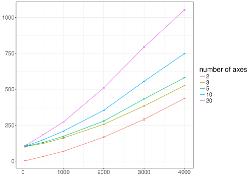
number of variables

Figure 1: Dataset from Mach et al. (2015). Running times averaged over 4 replicates of the PLNPCA function in R PLNmodels package. Single core Intel i7-4600U CPU 2.33GHz, R 3.4.1, Linux Ubuntu 16.04.

$\log_{10}(\text{abundance})$	$R^{2}$ criterion	chosen rank $\hat{q}$
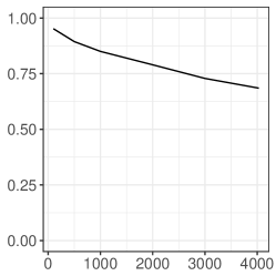
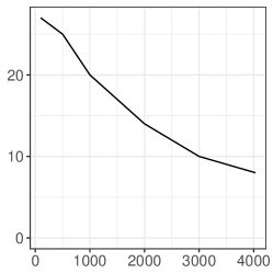
number of variables

Figure 2: Dataset from Mach et al. (2015). The minimum overall abundance of included OTUs (left panel), quality of approximation $R^{2}_{q}$ (central panel) and selected value $\hat{q}$ (right panel) decreases when OTUs with low abundance are added to the dataset.

Impact of Weaning

We focus on results obtained on the $500$ most abundant OTUs, which account for 90.3% of the total counts. We emphasize than even doing so, the count table remains quite sparse, with 67% of null counts and 60% of positive counts lower than or equal to $5$. The ICL criteria on this subset selects $\hat{q}=25$ ($R^{2}=89.4\%$). The main structure present in the latent subspace is the strong and systematic impact of weaning (Fig. 3, left), almost entirely captured by Axis 1. The variable factor map highlights OTUs from two specific bacterial families: Lactobacillaceae (red) and Prevotellaceae (blue). The former are typically found in dairy products and thought to be transmitted to the piglets via breast milk. As expected, they are enriched in suckling piglets and negatively correlated with Axis 1. The latter produce enzymes that are essential to degrade cereals introduced in the diet after weaning. As reported in Mach et al. (2015), they are enriched after weaning and positively correlated with Axis 1. The method is thus able to recover well known structures, cope with sparse count tables and account for varying sequencing depths.

Individual Factor Map                    Variable Factor Map

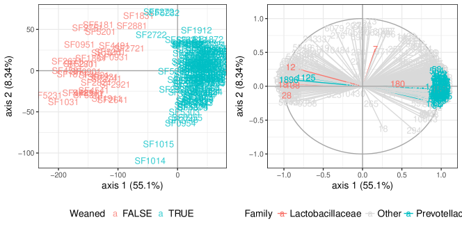
Figure 3: Individual (left) and variable (right) maps corresponding to the first principal plane of the $q$-dimensional approximation. Weaning has a strong and systematic effect on gut microbiota composition, well captured by axis 1. Bacterial families Prevotellaceae (red) and the Lactobacillaceae (blue) are two families well known to be affected by weaning and have a high correlation with Axis 1.

7.2 Oak powdery mildew pathobiome

Description of the experiment

We considered the metagenomic dataset introduced in Jakuschkin et al. (2016). Similarly to the Mach et al. (2015) dataset, it consists of microbial communities sampled on the surface of $n=116$ oak leaves. Communities were sequenced with both the hypervariable V6 region of 16S rRNA as marker-gene for bacteria and the ITS1 as marker-gene for fungi. Sequences were cleaned, clustered at the $97$% identity level to create OTUs and only the most abundant ones were kept (see Jakuschkin et al. (2016) for details of OTU picking and selection) resulting in a total of $p=114$ OTUs (66 bacterial ones and 44 fungal ones). One aim of this experiment is to understand the association between the abundance of the fungal pathogenic species E. alphitoides, responsible for the oak powdery mildew, and the other species. Furthermore, the leaves were collected on three trees with different resistance levels to the pathogen. In addition to the sampling tree, several covariates, all thought to potentially structure the community, were measured for each leaf: orientation, distance to ground, distance to trunk, direction, etc.

We emphasize that our goal slightly differs from the one of Jakuschkin et al. (2016) as these authors were interested in reconstructing the ecological network of the species, whereas our purpose is to summarize the species’ dependency structure in low dimension. Our approach also differs from a methodological view-point as we jointly estimate the effect of the covariates $\boldsymbol{\Theta}$ and the dependency structure $\boldsymbol{\Sigma}$ while they first corrected the observed counts for the effect of the covariates using a regression model before feeding the residuals from that regression to a network inference method. This two-steps procedure fails both to account for the fact that $\boldsymbol{\Theta}$ is estimated and to propagate uncertainty from the first step to the second one.

	Offset ($M_{0}$)                                Offset and covariates ($M_{1}$)
criterion value
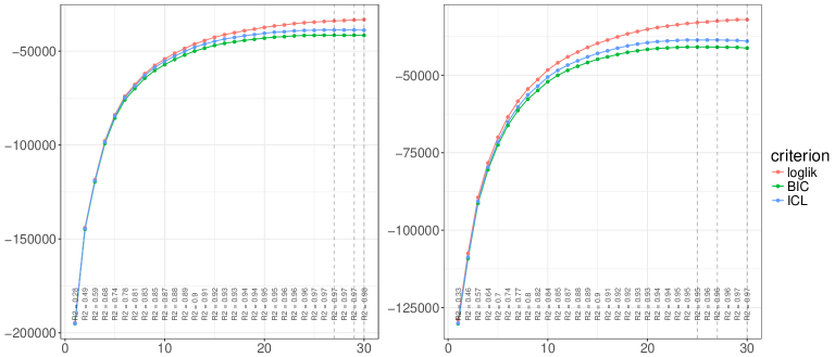
	number of axes

(a) Model selection

	$R_{q}^{2}$ criterion                         Entropy ($\mathrm{BIC}_{q}-\mathrm{ICL}_{q}$)
criterion value
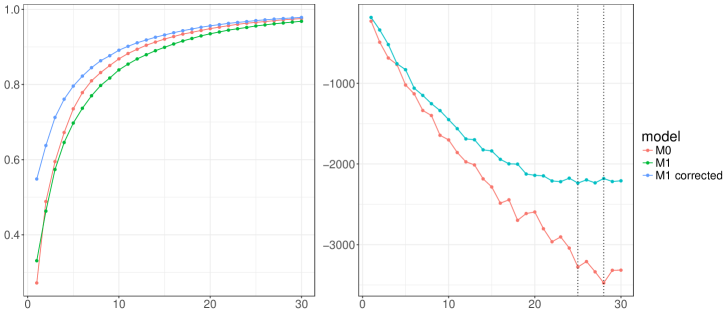
	number of axes

(b) Goodness of fit and Entropy

Figure 4: Dataset from Jakuschkin et al. (2016). $(a)$ model selection criteria $J_{q}$, $BIC_{q}$ and $ICL_{q}$ for model $M_{0}$ (left) and $M_{1}$ (right); $(b)$ $R^{2}_{q}$ criterion and entropy of $\widetilde{p}(\boldsymbol{W})$

Offset ($M_{0}$)                                     Offset and covariates ($M_{1}$)

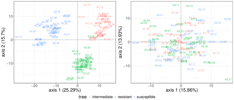
(a) Individual Factor Maps and tree status

Offset ($M_{0}$)                                     Offset and covariates ($M_{1}$)

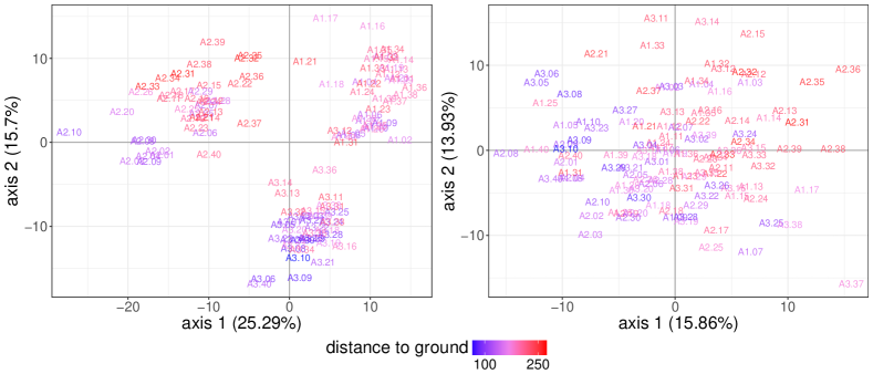
(b) Individual Factor Maps and distance to ground

Figure 5: Dataset from Jakuschkin et al. (2016). Scatter plot of the leaves on the first two principal components (left: $M_{0}$, right: $M_{1}$) with colors corresponding to either tree status $(a)$ or distance to ground $(b)$. Accounting for tree status reveals an ecological gradient along distance to ground.

Importance of the offset

The abundances $Y_{ij}$ (where $i$ denotes the leaf and $j$ the OTUs) were measured separately for fungi and bacteria resulting in different sampling efforts for the two types of OTUs: the median total abundance were respectively 668 for bacteria and 2166 for fungi. To account for this, we define a different offset $O_{ij}$ term for each OTU type. Offsets are still computed as the log-total sums of reads, including those of filtered out OTUs, for each OTU type.

Model selection

The three trees from which the leafs where collected were respectively susceptible, intermediately resistant (hereafter “intermediate”) and resistant to mildew. We first fitted a null Poisson-lognormal model $M_{0}$ as defined in (9) with only an offset term. Alternatively, we considered model $M_{1}$ involving two covariates: the tree from which each leaf was collected from, and the orientation (0=south-east, 1=north-west) of its branch.

Figure 4a displays the lower bound $J$, the BIC and the ICL for model $M_{0}$ (left) and $M_{1}$ (right) as a function of the number of axes $q$ considered. We observe that the $J_{q}$ is always increasing and that both BIC and ICL criteria behave similarly. According to the ICL criterion, we selected $\widehat{q}_{0}=28$ ($ICL=-38,619$) latent dimensions for model $M_{0}$ and $\widehat{q}=25$ ($ICL=-38,472$) for model $M_{1}$. This suggest that the two models (with their respective optimal dimension) provide a very similar fit.

We looked at the approximate posterior entropy in panel left of Figure 4b: we observed that it is minimal near to the respective optimum in terms of model selection. This indicates that the selected dimensions are also optimal in terms of uncertainty on the latent variables.

Effect of the covariates

The choice between model $M_{0}$ and $M_{1}$ is mostly a matter of the type of dependency we analyze with each of them, as the former does not account for the covariates whereas the latter does. This is illustrated in Figure 5a (top), when plotting the first principal plane. In model $M_{0}$ (left), the leafs collected on each tree are clearly separated. As expected, taking the tree as a covariate (right) removes the tree effect from the principal plane.

Adding covariates in the model also allows us to explore second-order structuring effects that are masked by the strong first-order effect of the sampling tree. Figure 5a (bottom) thus shows that in addition to sampling tree, communities are structured by the distance of the leaf to the ground. The effect of covariates on the abundance of E. alphitoides were also consistent: the estimated parameters $\theta_{ij}$ associated with the intermediate and resistant trees were $-3.94$ and $-7.05$, respectively, taking the susceptible tree as a reference.

We compared the respective estimates of $\boldsymbol{\Sigma}$ under $M_{0}$ (denoted $\widehat{\boldsymbol{\Sigma}}_{0}$) and under $M_{1}$ ($\widehat{\boldsymbol{\Sigma}}_{1}$) focusing on the correlations between E. alphitoides and the other OTUs. $\widehat{\boldsymbol{\Sigma}}_{0}$ contains correlations between OTUs that are either due to marginal co-variations between them or to the effect of the covariates, whereas the correlations in $\widehat{\boldsymbol{\Sigma}}_{1}$ are corrected from the effect of covariates. We first observed a reduction of the variances (median=.175, mean=.303 in $\widehat{\boldsymbol{\Sigma}}_{0}$; median=.087, mean=.176 in $\widehat{\boldsymbol{\Sigma}}_{1}$), which proves the strong effect of covariates on the abundance of the different OTUs. We then ranked all species according to their correlation with the pathogene and found very different rankings $M_{0}$ and $M_{1}$ (Kendall’s $\tau=.41$), showing that the covariates drastically change the apparent relationship between OTU abundances.

Percentage of variance

We now comment on use of the $R_{q}^{2}$ criterion defined in Section 6 to evaluate the proportion of variability captured by a model with $q$ latent dimensions. $R_{q}^{2}$ compares the pseudo-likelihood $\ell_{q}^{m}$ obtained with $q$ latent dimensions under model $M_{m}$ ($m=0,1$) with the likelihoods $\ell_{\min}^{m}$ and $\ell_{\max}^{m}$. We know that $\ell_{\max}^{0}=\ell_{\max}^{1}$ whereas $\ell_{\min}^{0}<\ell_{\min}^{1}$ because $\ell_{\min}^{0}$ only relies on the offsets whereas $\ell_{\min}^{1}$ accounts for both the offsets and the covariates. As a consequence, $R_{q}^{2}$ tends to be higher under $M_{0}$ than under $M_{1}$ for a given $q$. Right panel of Figure 4b compares the genuine $R_{q}^{2}$ under models $M_{0}$ and $M_{1}$ and the corrected version of $R_{q}^{2}$ under model $M_{1}$ using $\ell_{\min}^{0}$ in place of $\ell_{\min}^{1}$. As expected, the corrected version of $R_{q}^{2}$ is always higher under $M_{1}$ than under $M_{0}$. We also observe that, for both models, the proportion of variability captured by the latent space is quite high: $R_{28}^{2}=97.21\%$ for $M_{0}$ and $R_{25}^{2}=97.02\%$ for $M_{1}$. We remind that $\widehat{q}_{0}=28$ and $\widehat{q}_{1}=25$ should both be compared with $p=114$.

Variance of the variational conditional distribution

We remind that $S_{ij}$ is the approximate conditional standard deviation of $W_{ij}$ given the data. This parameter measures the precision of the location of individual $i$ along the $j$-th latent dimension. We can derive from them the approximate conditional variance of each $Z_{ij}$ as $[\boldsymbol{B}\operatorname*{diag}(\boldsymbol{s}_{i}\odot\boldsymbol{s}_{i})\boldsymbol{B}^{\intercal}]_{jj}$. Figure 6 shows that this variance is much higher when the corresponding abundance $Y_{ij}$ is low. Indeed, any large negative values of $Z_{ij}$ yields a Poisson parameter close to zero and in turn a null $Y_{ij}$. As a consequence, large negative $Z_{ij}$ cannot be predicted accurately. This is a natural consequence of the non-linear nature of the exponential transform: large swaths of the parameter space are compressed to small regions of the observation space.

approximate conditional standard error of $Z_{ij}$

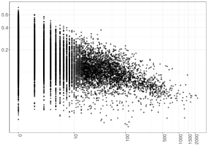
$Y_{ij}$ (log scale)

Figure 6: Variational approximate conditional standard error of the $Z_{ij}$ ($y$ axis) as a function of the abundance $Y_{ij}$ ($x$ axis).

Acknowledgement

We thank Corinne Vacher and Nuria Mach for providing the data and discussing the results. Two anonymous reviewers gave insightful comments that helped improve the quality of this manuscript. We also thank Charlie Pauvert for his feedback on the code and Elsa Teulière for finding extra typos in the paper.

This work partially was funded by ANR Hydrogen (project ANR-14-CE23-0001) and Inra MEM Metaprogramme (Meta-omics and microbial ecosystems, projects LearnBioControl and Brassica-Dev).

Appendix A Convexity Lemmas

Lemma 1.

For any vectors $\boldsymbol{\theta}$, $\boldsymbol{x}$, $\boldsymbol{m}$, $\boldsymbol{s}$ and $\boldsymbol{b}$ (with matching dimensions) and convex function $f$, if $\boldsymbol{u}\sim\mathcal{N}(0,\boldsymbol{I})$ and $\boldsymbol{w}=\boldsymbol{m}+\boldsymbol{s}\odot\boldsymbol{u}\sim\mathcal{N}(\boldsymbol{m},\operatorname*{diag}(\boldsymbol{s}\odot\boldsymbol{s}))$, then the map $g:(\boldsymbol{\theta},\boldsymbol{m},\boldsymbol{s},\boldsymbol{b})\mapsto\mathbb{E}[f(\boldsymbol{\theta}^{\intercal}\boldsymbol{x}+\boldsymbol{b}^{\intercal}\boldsymbol{w})]$ is convex in $(\boldsymbol{\theta},\boldsymbol{b})$ for $(\boldsymbol{m},\boldsymbol{s})$ fixed and vice-versa.

Proof.

Note $Z=\boldsymbol{\theta}^{\intercal}\boldsymbol{x}+\boldsymbol{b}^{\intercal}\boldsymbol{w}=(\boldsymbol{\theta}^{\intercal}\boldsymbol{x}+\boldsymbol{b}^{\intercal}\boldsymbol{m})+\boldsymbol{b}^{\intercal}(\boldsymbol{s}\odot\boldsymbol{u})$. The first order derivative of $g$ is

$$\boldsymbol{\nabla}(\boldsymbol{\theta},\boldsymbol{b},\boldsymbol{m},\boldsymbol{s})=\mathbb{E}\left[f^{\prime}(Z)\begin{bmatrix}\boldsymbol{x}&\boldsymbol{m}+\boldsymbol{s}\odot\boldsymbol{u}&\boldsymbol{b}&\boldsymbol{b}\odot\boldsymbol{u}\end{bmatrix}^{\intercal}\right].$$

The second order partial derivatives of $g$ are:

$$\boldsymbol{\Psi}_{1}(\boldsymbol{\theta},\boldsymbol{b}) =\mathbb{E}\left[f^{\prime\prime}(Z)\begin{bmatrix}\boldsymbol{x}\boldsymbol{x}^{\intercal}&\boldsymbol{x}(\boldsymbol{m}+\boldsymbol{u}\odot\boldsymbol{s})^{\intercal}\\ (\boldsymbol{m}+\boldsymbol{s}\odot\boldsymbol{u})\boldsymbol{x}^{\intercal}&(\boldsymbol{m}+\boldsymbol{s}\odot\boldsymbol{u})(\boldsymbol{m}+\boldsymbol{s}\odot\boldsymbol{u})^{\intercal}\\ \end{bmatrix}\right]$$

$$\boldsymbol{\Psi}_{2}(\boldsymbol{m},\boldsymbol{s}) =\mathbb{E}\left[f^{\prime\prime}(Z)\begin{bmatrix}\boldsymbol{b}\boldsymbol{b}^{\intercal}&\boldsymbol{b}(\boldsymbol{b}\odot\boldsymbol{u})^{\intercal}\\ (\boldsymbol{b}\odot\boldsymbol{u})\boldsymbol{b}^{\intercal}&(\boldsymbol{b}\odot\boldsymbol{u})(\boldsymbol{b}\odot\boldsymbol{u})^{\intercal}\\ \end{bmatrix}\right]$$

And the associated quadratic form $\Phi_{1}(\boldsymbol{v},\boldsymbol{w})=(\boldsymbol{v},\boldsymbol{w})^{\intercal}\boldsymbol{\Psi}_{1}(\boldsymbol{\theta},\boldsymbol{b})(\boldsymbol{v},\boldsymbol{w})$ and $\Phi_{2}(\boldsymbol{v},\boldsymbol{w})=(\boldsymbol{v},\boldsymbol{w})^{\intercal}\boldsymbol{\Psi}_{2}(\boldsymbol{m},\boldsymbol{s})(\boldsymbol{v},\boldsymbol{w})$ can be simplified to

$$\Phi_{1}(\boldsymbol{v},\boldsymbol{w}) =\mathbb{E}[f^{\prime\prime}(Z)(\boldsymbol{x}^{\intercal}\boldsymbol{v}+(\boldsymbol{m}+\boldsymbol{s}\odot\boldsymbol{u})^{\intercal}\boldsymbol{w})^{2}]\geq 0$$

$$\Phi_{2}(\boldsymbol{v},\boldsymbol{w}) =\mathbb{E}[f^{\prime\prime}(Z)(\boldsymbol{b}^{\intercal}\boldsymbol{v}+(\boldsymbol{b}\odot\boldsymbol{u})^{\intercal}\boldsymbol{w})^{2}]\geq 0$$

The Hessians $\boldsymbol{\Psi}_{1}$ and $\boldsymbol{\Psi}_{2}$ are thus semidefinite positive, which ends the proof. ∎

Lemma 2.

For any matrices $\boldsymbol{\Theta}$, $\boldsymbol{X}$, $\boldsymbol{M}$, $\boldsymbol{S}$ and $\boldsymbol{B}$ (with matching dimensions) and convex function $f$, if $\boldsymbol{U}=[\boldsymbol{U}_{1},\dots,\boldsymbol{U}_{n}]^{\intercal}$ where the $\boldsymbol{U}_{i}$ are i.i.d and $\boldsymbol{U}_{i}\sim\mathcal{N}(\boldsymbol{0},\boldsymbol{I})$ and $\boldsymbol{W}=\boldsymbol{M}+\boldsymbol{S}\odot\boldsymbol{U}$. The map $g:(\boldsymbol{\Theta},\boldsymbol{M},\boldsymbol{S},\boldsymbol{B})\mapsto\boldsymbol{1}^{\intercal}_{n}\mathbb{E}[f(\boldsymbol{X}\boldsymbol{\Theta}^{\intercal}+\boldsymbol{W}\boldsymbol{B}^{\intercal})]\boldsymbol{1}_{p}$ is convex in $(\boldsymbol{\Theta},\boldsymbol{B})$ for $(\boldsymbol{M},\boldsymbol{S})$ fixed and vice-versa.

Proof.

The function $g$ is a sum of functions of the form $g_{ij}:(\boldsymbol{\Theta},\boldsymbol{M},\boldsymbol{S},\boldsymbol{B})\mapsto\mathbb{E}[f(\boldsymbol{X}^{\intercal}_{i}\boldsymbol{\Theta}_{j}+\boldsymbol{B}^{\intercal}_{j}(\boldsymbol{M}_{i}+\boldsymbol{S}_{i}\odot\boldsymbol{U})]$. The result follows from Lemma 1. ∎

References

- Acharya et al. (2015) A. Acharya, J. Ghosh, and M. Zhou. Nonparametric bayesian factor analysis for dynamic count matrices. In AISTATS, 2015.
- Aitchison and Ho (1989) John Aitchison and CH Ho. The multivariate poisson-log normal distribution. Biometrika, 76(4):643–653, 1989.
- Anderson (2003) T. W. Anderson. An introduction to multivariate statistical analysis. Series in Probability and Statistics. Wiley, 3 edition, 2003.
- Biernacki et al. (2000) C. Biernacki, G. Celeux, and G. Govaert. Assessing a mixture model for clustering with the integrated completed likelihood. IEEE Trans. Pattern Anal. Machine Intel., 22(7):719–25, 2000.
- Cao and Xie (2015) Y. Cao and Y. Xie. Poisson matrix completion. In 2015 IEEE International Symposium on Information Theory (ISIT), pages 1841–1845. IEEE, 2015.
- Chen et al. (2017) Jun Chen, Emily King, Rebecca Deek, Zhi Wei, Yue Yu, Diane Grill1, and Karla Ballman. An omnibus test for differential distribution analysis of microbiome sequencing data. Bioinformatics, page btx650, 2017. 10.1093/bioinformatics/btx650.
- Collins et al. (2001) M. Collins, S. Dasgupta, and R. E Schapire. A generalization of principal components analysis to the exponential family. In Advances in neural information processing systems, pages 617–624, 2001.
- Dempster et al. (1977) A. P. Dempster, N. M. Laird, and D. B. Rubin. Maximum likelihood from incomplete data via the EM algorithm. J. R. Statist. Soc. B, 39:1–38, 1977.
- Eckart and Young (1936) C. Eckart and G. Young. The approximation of one matrix by another of lower rank. Psychometrika, 1(3):211–218, 1936.
- Gloor et al. (2017) Gregory B. Gloor, Jean M. Macklaim, Vera Pawlowsky-Glahn, and Juan J. Egozcue. Microbiome datasets are compositional: And this is not optional. Frontiers in Microbiology, 8:2224, 2017. ISSN 1664-302X. 10.3389/fmicb.2017.02224. URL https://www.frontiersin.org/article/10.3389/fmicb.2017.02224.
- Hall et al. (2011) P. Hall, J. T Ormerod, and MP Wand. Theory of gaussian variational approximation for a Poisson mixed model. Statistica Sinica, pages 369–389, 2011.
- Izsák (2008) R. Izsák. Maximum likelihood fitting of the Poisson log-normal distribution. Environmental and Ecological Statistics, 15(2):143–156, 2008.
- Jaakkola and Jordan (2000) T. S. Jaakkola and M. I. Jordan. Bayesian parameter estimation via variational methods. Statistics and Computing, 10(1):25–37, 2000.
- Jakuschkin et al. (2016) B. Jakuschkin, V. Fievet, L. Schwaller, T. Fort, C. Robin, and C. Vacher. Deciphering the pathobiome: Intra-and interkingdom interactions involving the pathogen Erysiphe alphitoides. Microbial ecology, pages 1–11, 2016.
- Johnson et al. (1997) N. L. Johnson, S. Kotz, and N. Balakrishnan. Discrete multivariate distributions, volume 165. Wiley New York, 1997.
- Johnson (2011) Steven G Johnson. The NLopt nonlinear-optimization package, 2011. URL http://ab-initio.mit.edu/nlopt.
- Karlis (2005) D. Karlis. EM algorithm for mixed Poisson and other discrete distributions. Astin bulletin, 35(01):3–24, 2005.
- Lafond (2015) J. Lafond. Low rank matrix completion with exponential family noise. arXiv preprint arXiv:1502.06919, 2015.
- Landgraf (2015) A. J Landgraf. Generalized Principal Component Analysis: Dimensionality Reduction through the Projection of Natural Parameters. PhD thesis, The Ohio State University, 2015.
- Lee and Seung (2001) D. D Lee and H S. Seung. Algorithms for non-negative matrix factorization. In Advances in neural information processing systems, pages 556–562, 2001.
- Li and Tao (2010) J. Li and D. Tao. Simple exponential family PCA. In AISTATS, pages 453–460, 2010.
- Little and Rubin (2014) Roderick JA Little and Donald B Rubin. Statistical analysis with missing data. John Wiley & Sons, 2014.
- Liu et al. (2016) L. T. Liu, E. Dobriban, and A. Singer. PCA: High Dimensional Exponential Family PCA. ArXiv e-prints arXiv:1611.05550, 2016.
- Mach et al. (2015) N. Mach, M. Berri, J. Estellé, F. Levenez, G. Lemonnier, C. Denis, J.-J. Leplat, C. Chevaleyre, Y. Billon, J. Doré, C. Rogel-Gaillard, and P. Lepage. Early-life establishment of the swine gut microbiome and impact on host phenotypes. Environmental Microbiology Reports, 7(3):554–569, May 2015. 10.1111/1758-2229.12285.
- Mardia et al. (1979) K.V. Mardia, J.T. Kent, and J.M. Bibby. Multivariate analysis. Academic press, 1979.
- Minka (2000) T. P Minka. Automatic choice of dimensionality for PCA. In NIPS, volume 13, pages 598–604, 2000.
- Mohamed et al. (2009) S. Mohamed, Z. Ghahramani, and K. A Heller. Bayesian exponential family PCA. In Advances in neural information processing systems, pages 1089–1096, 2009.
- Nelson (1985) J. F Nelson. Multivariate gamma-poisson models. Journal of the American Statistical Association, 80(392):828–834, 1985.
- Press et al. (1989) William H Press, Brian P Flannery, Saul A Teukolsky, William T Vetterling, et al. Numerical recipes. cambridge University Press, cambridge, third edition edition, 1989.
- R Development Core Team (2008) R Development Core Team. R: A Language and Environment for Statistical Computing. R Foundation for Statistical Computing, Vienna, Austria, 2008. URL http://www.R-project.org. ISBN 3-900051-07-0.
- Royle and Wikle (2005) J A. Royle and C. K Wikle. Efficient statistical mapping of avian count data. Environmental and Ecological Statistics, 12(2):225–243, 2005.
- Salmon et al. (2014) J. Salmon, Z. Harmany, C.-A. Deledalle, and R. Willett. Poisson noise reduction with non-local PCA. Journal of mathematical imaging and vision, 48(2):279–294, 2014.
- Schwarz (1978) G. Schwarz. Estimating the dimension of a model. Ann. Statist., 6:461–4, 1978.
- Smets et al. (2015) Wenke Smets, Jonathan W Leff, Mark A Bradford, Rebecca L McCulley, Sarah Lebeer, and Noah Fierer. A method for simultaneous measurement of soil bacterial abundances and community composition via 16s rrna gene sequencing. PeerJ PrePrints, 3:e1622, 8 2015. ISSN 2167-9843. 10.7287/peerj.preprints.1318v1. URL https://dx.doi.org/10.7287/peerj.preprints.1318v1.
- Srivastava and Chen (2010) S. Srivastava and L. Chen. A two-parameter generalized Poisson model to improve the analysis of RNA-seq data. Nucleic acids research, 38(17):e170–e170, 2010.
- Svanberg (2002) K. Svanberg. A class of globally convergent optimization methods based on conservative convex separable approximations. SIAM journal on optimization, 12(2):555–573, 2002.
- Tipping and Bishop (1999) M. E Tipping and C. M Bishop. Probabilistic principal component analysis. Journal of the Royal Statistical Society: Series B (Statistical Methodology), 61(3):611–622, 1999.
- Tsilimigras and Fodor (2016) Matthew C.B. Tsilimigras and Anthony A. Fodor. Compositional data analysis of the microbiome: fundamentals, tools, and challenges. Annals of Epidemiology, 26(5):330 – 335, 2016. ISSN 1047-2797. https://doi.org/10.1016/j.annepidem.2016.03.002. URL http://www.sciencedirect.com/science/article/pii/S1047279716300722. The Microbiome and Epidemiology.
- Vandeputte et al. (2017) Doris Vandeputte, Gunter Kathagen, Kevin D’hoe, Sara Vieira-Silva, Mireia Valles-Colomer, João Sabino, Jun Wang, Raul Y Tito, Lindsey De Commer, Youssef Darzi, et al. Quantitative microbiome profiling links gut community variation to microbial load. Nature, 551(7681), 2017. URL https://www.nature.com/articles/nature24460.
- Wainwright and Jordan (2008) M. J. Wainwright and M. I. Jordan. Graphical models, exponential families, and variational inference. Found. Trends Mach. Learn., 1(1–2):1–305, 2008.
- Wickham (2009) Hadley Wickham. ggplot2: Elegant Graphics for Data Analysis. Springer-Verlag New York, 2009. ISBN 978-0-387-98140-6. URL http://ggplot2.org.
- Witten et al. (2009) D. M Witten, R. Tibshirani, and T. Hastie. A penalized matrix decomposition, with applications to sparse principal components and canonical correlation analysis. Biostatistics, 2009.
- Ypma (2017) Jelmer Ypma. R interface to nlopt, v. 1.0.4. https://github.com/jyypma/nloptr, 2017.
- Zhou (2016) M. Zhou. Nonparametric bayesian negative binomial factor analysis. arXiv preprint arXiv:1604.07464, 2016.
- Zhou et al. (2012) M. Zhou, L. Hannah, D. B Dunson, and L. Carin. Beta-negative binomial process and poisson factor analysis. In AISTATS, volume 22, pages 1462–1471, 2012.