Non-integrability of the semiclassical Jaynes–Cummings models without the rotating-wave approximation

Abstract

Two versions of the semi-classical Jaynes–Cummings model without the rotating wave approximation are investigated. It is shown that for a non-zero value of the coupling constant the version introduced by Belobrov, Zaslavsky, and Tartakovsky is Hamiltonian with respect to a certain degenerated Poisson bracket. Moreover, it is shown that both models are not integrable.

1 Introduction

The Jaynes–Cummings model describes a system of $n$ two-levels atoms interacting with a single mode of the electromagnetic field. Its rotating-wave approximation is exactly solvable. With this approximation, its semi-classical version is also solvable. On the other hand, numerical investigations of the semi-classical version of the Jaynes–Cummings model without the rotating wave approximation shows its chaotic behaviour for a large range of its parameters. Nevertheless, particular periodic solutions of this system were found analytically.

Till now an integrability analysis of this system was not performed. Here we investigate this problem in the framework of differential Galois theory.

There are two version of the the semi-classical Jaynes–Cummings system. The first of them, investigated in [1] has the following form

$$\dot{x} =-y$$ (1.1a)

$$\dot{y} =x+zE,$$ (1.1b)

$$\dot{z} =-yE,$$ (1.1c)

$$\dot{E} =B,$$ (1.1d)

$$\dot{B} =\alpha x-\mu^{2}E,$$ (1.1e)

where $\mu=\omega/\omega_{0}$ and $\alpha=n\mu(2\lambda/\omega_{0})^{2}$ are the dimensionless parameters, and the dot denotes the derivative with respect to rescaled time $\tau=\omega_{0}t$. Here $\omega_{0}$ is the transition frequency of each atom and $n$ is the number of two level atoms. It is easy to verify that the system (1.1) posses two first integrals

$$F=x^{2}+y^{2}+z^{2},$$ (1.2)

and the energy integral

$$H=\alpha z-\alpha xE+\frac{1}{2}\mu^{2}E^{2}+\frac{1}{2}B^{2}.$$ (1.3)

Jeleńska-Kuklińska in  [4], and Kujawski in [7, 8], found exact solutions of the system (1.1). They can be expressed in terms of elliptic Jacobian function

$$E=E_{0}\operatorname{cn}(\Omega t,m),$$ (1.4)

where

$$\Omega^{2}=\pm\frac{1}{2}\left(\mu^{2}-\frac{1}{3}\right)\sqrt{1+\chi},$$ (1.5)

$$m=\frac{1}{2}+\frac{\mu^{2}-\frac{1}{3}}{4\Omega^{2}},\quad E_{0}^{2}=16m\Omega^{2},$$ (1.6)

and

$$\chi=\left(\mu^{2}-\frac{1}{3}\right)^{-2}\left\{\pm\frac{4}{3}\sqrt{\alpha^{2}-4\left(\mu^{2}-\frac{1}{9}\right)^{3}}-\left(\mu^{2}-\frac{1}{9}\right)\left(\mu^{2}-\frac{17}{9}\right)\right\}.$$ (1.7)

Solution (1.4) lies on energy level $H((x,y,z,E,B)=h$ with

$$h=\pm\frac{5}{3}\sqrt{\alpha^{2}-4\left(\mu^{2}-\frac{1}{9}\right)^{3}}-2\left(\mu^{2}-\frac{1}{9}\right)\left(\mu^{2}-\frac{5}{9}\right).$$ (1.8)

The components of the Bloch vector given in terms of the electric field $E$ are defined by

$$\begin{split}x(E)&=\frac{1}{\alpha}\left[\frac{3}{2}\left(\mu^{2}-\frac{1}{9}\right)E-\frac{1}{8}E^{3}\right],\qquad y(E)=-\dot{x}(E),\\ z(E)&=\frac{1}{\alpha}\left[-\frac{3}{2}\left(\mu^{2}-\frac{1}{9}\right)^{2}\pm\sqrt{\alpha^{2}-4\left(\mu^{2}-\frac{1}{9}\right)^{3}}+\frac{3}{4}\left(\mu^{2}-\frac{1}{9}\right)E^{2}-\frac{3}{32}E^{4}\right].\end{split}$$ (1.9)

The domain of parameters for which solution (1.4) is real can be easily determined from the above formulae.

Since the system (1.1) posses two first integrals (1.2) and (1.3) we are able to reduce the dimension of the phase space to three. Hence in order to get quickly insight into the dynamics of the considered system we make the Poincaré cross sections, which are shown in Figs. 1-2. The black bullets denotes the elliptic solutions described enough. Although the Poincaré cross section is a standard tool for study chaotic dynamics, we did not find its application in previous study of the Jaynes–Cummings system.

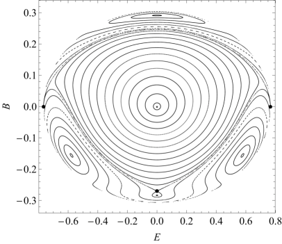
(a) $\mu=\frac{2}{5},\ \alpha=\frac{44}{1875},\ h=\frac{44}{1875}$

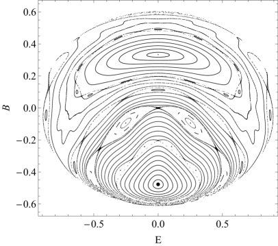
(b) $\mu=\frac{2}{3},\ \alpha=0.43,\ h=\frac{1}{540}\left(40-\sqrt{29769}\right)$

Figure 1: Poincaré sections on the surface $x=0$ with $y>0$ and $z\in\mathbb{R}$ restricted to the plane $(E,B)$

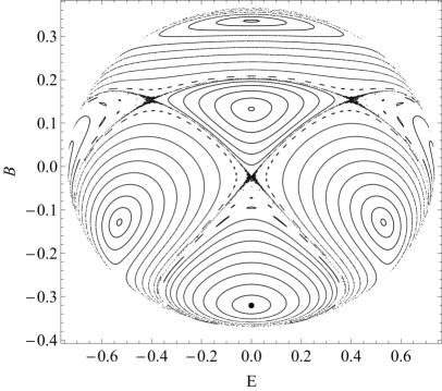
(a) $\mu=\frac{1}{2},\ \alpha=0.42,\ h=\frac{55}{648}-\frac{\sqrt{64759}}{1620}$

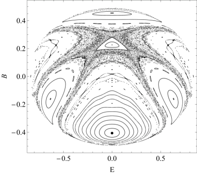
(b) $\mu=\frac{\sqrt{3}}{3},\ \alpha=\frac{1}{4},\ h=\frac{8}{81}-\frac{5\sqrt{217}}{324}$

Figure 2: Poincaré sections on the surface $x=0$ with $y>0$ and $z\in\mathbb{R}$ restricted to the plane $(E,B)$

Here we would like to point out the system (1.1) is Hamiltonian with respect to a certain degenerated Poisson structure in $\mathbb{R}^{5}$. To see this let us assume that $\alpha\neq 0$. Then, we can rewrite system (1.1) in the following form

$$\dot{\boldsymbol{q}}=\boldsymbol{J}(\boldsymbol{q})H^{\prime}(\boldsymbol{q}),\qquad\boldsymbol{q}=[x,y,z,E,B]^{T},$$ (1.10)

where

$$\boldsymbol{J}(\boldsymbol{q}):=\frac{1}{\alpha}\begin{bmatrix}0&z&-y&0&0\\ -z&0&x&0&0\\ y&-x&0&0&0\\ 0&0&0&0&\alpha\\ 0&0&0&-\alpha&0\end{bmatrix}$$ (1.11)

The Poisson bracket defined by $\boldsymbol{J}(\boldsymbol{q})$ is degenerated. First integral $F(\boldsymbol{q})$ is the Casimir of this bracket.

If $\alpha=0$ then system (1.1) in can be written the following form

$$\dot{\boldsymbol{q}}=\boldsymbol{J}_{0}(\boldsymbol{q})K^{\prime}(\boldsymbol{q}),\qquad K(\boldsymbol{q})=\frac{1}{2}F(\boldsymbol{q})+H(\boldsymbol{q})$$ (1.12)

where

$$\boldsymbol{J}_{0}(\boldsymbol{q}):=\begin{bmatrix}0&-1&0&0&0\\ 1&0&E&0&0\\ 0&-E&0&0&0\\ 0&0&0&0&1\\ 0&0&0&-1&0\end{bmatrix}$$ (1.13)

Although this matrix is antisymmetric it does not define the Poisson structure as the bracket which it defines does not satisfied the Jacobi identity.

The different version of the system (1.1) has been studied by Miloni and co-workers, see [9]. Namely

$$\dot{x} =-y$$ (1.14a)

$$\dot{y} =x+zE,$$ (1.14b)

$$\dot{z} =-yE,$$ (1.14c)

$$\dot{E} =B,$$ (1.14d)

$$\dot{B} =\alpha(x+zE)-\mu^{2}E,$$ (1.14e)

where the dimensionless parameters $\mu,\alpha$ have the same meaning as in the first case. Authors have presented the complexity of the system by means of Fourier analysis as well as by maximal Lyapunov exponent.

We found that this version of the Jaynes–Cummings model has also two constants of motion

$$F=x^{2}+y^{2}+z^{2},\qquad H_{\mathrm{M}}=\frac{1}{2}\alpha^{2}y^{2}-\alpha yB+\alpha\mu^{2}z+\frac{1}{2}\mu^{2}E^{2}+\frac{1}{2}B^{2}.$$ (1.15)

The existence of the first integral $H_{\mathrm{M}}$ was not reported in it earlier studies of this system. Although it looks quite similar to system (1.1) we were not able to find any particular solution on the sphere $x^{2}+y^{2}+z^{2}=1$. More importantly, it is seems this system cannot be written as a Hamiltonian system with respect to a degenerated Poisson structure. Nevertheless, we have found that it can be put in the following form

$$\dot{\boldsymbol{q}}=\boldsymbol{P}(\boldsymbol{q})H^{\prime}_{\mathrm{M}}(\boldsymbol{q}),$$ (1.16)

where

$$\boldsymbol{P}(\boldsymbol{q}):=\frac{1}{\alpha\mu^{2}}\begin{bmatrix}0&0&-y&0&0\\ 0&0&x&\alpha z&0\\ y&-x&0&-\alpha y&-\alpha x\\ 0&-\alpha z&\alpha y&0&-\alpha(\alpha z-\mu^{2})\\ 0&0&\alpha x&\alpha(\alpha z-\mu^{2})&0\end{bmatrix}$$ (1.17)

Figure 3 and 4 show the complexity of the system. We made the Poincaré cross sections for the exact resonance, when $\mu=1$ and $\alpha=1$ for gradually increasing value of energy. As we can see, for higher and higher values of energy the dynamics becomes more and more complex, see especially Figure 4 presenting the high stage of chaotic behaviour.

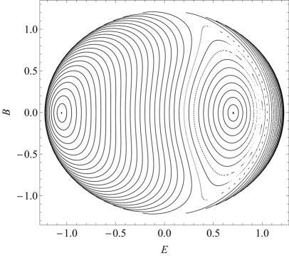
(a) $\mu=1,\ \alpha=1,\ h=-0.5$

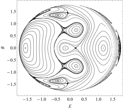
(b) $\mu=1,\ \alpha=1,\ h=1.2$

Figure 3: Poincaré sections on the surface $x=0$ with $y>0$ and $z\in\mathbb{R}$ restricted to the plane $(E,B)$

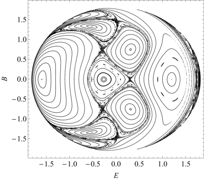
(a) $\mu=1,\ \alpha=1,\ h=1.3$

.

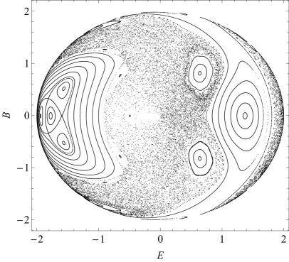
(b) $\mu=1,\ \alpha=1,\ h=2$

Figure 4: Poincaré sections on the surface $x=0$ with $y>0$ and $z\in\mathbb{R}$ restricted to the plane $(E,B)$

As we see, the numerical analysis shows that the dynamics of the both systems (1.1) and  (1.14) is very complex and in fact chaotic. Thus, our main goal of this article is to prove that these systems are not integrable. More precisely, we show that they do not admit additional meromorphic first integral. The main result is formulated in the following theorem.

Theorem 1.1.

For $\mu\neq 0$, systems (1.1) and  (1.14) do not have an additional meromorphic first which is functionally independent with the respective known two first integrals.

2 Proof of Theorem 1.1

Both systems (1.1) and (1.14) have the same invariant manifold defined by

$${\mathscr{N}}=\left\{(x,y,z,E,B)\in\mathbb{C}^{5}|x=y=z=0\right\}$$ (2.1)

and its restriction to ${\mathscr{N}}$ is defined by

$$\dot{E}=B,\qquad\dot{B}=-\mu^{2}E.$$ (2.2)

Hence, solving equation (2.2) we obtain a particular solution

$$\boldsymbol{\varphi}(t)=(0,0,0,E(t),B(t)),\quad E(t)=\cos\mu t,\quad B(t)=-\mu\sin\mu t,$$ (2.3)

Let $(\xi_{1},\xi_{2},\xi_{3},\eta_{1},\eta_{2})^{T}$ be the variation of $(x,y,z,E,B)^{T}$, then the variational equations along the particular solution (2.3) for system (1.1) takes the following matrix form

$$\begin{pmatrix}\dot{\xi}_{1}\\ \dot{\xi}_{2}\\ \dot{\xi}_{3}\\ \dot{\eta}_{1}\\ \dot{\eta}_{2}\\ \end{pmatrix}=\begin{pmatrix}0&-1&0&0&0\\ 1&0&\cos\mu t&0&0\\ 0&-\cos\mu t&0&0&0\\ 0&0&0&0&1\\ \alpha&0&0&-\mu^{2}&0\\ \end{pmatrix}\begin{pmatrix}\xi_{1}\\ \xi_{2}\\ \xi_{3}\\ \eta_{1}\\ \eta_{2}\end{pmatrix}.$$ (2.4)

Since the motion takes place on the $(E,B)$ plane, equations for $(\xi_{1},\xi_{2},\xi_{2})$ form a subsystem of the normal variational equations

$$\dot{\xi}_{1}=-\xi_{2},\quad\dot{\xi}_{2}=\xi_{1}+\xi_{3}\cos\mu t,\quad\dot{\xi}_{3}=-\xi_{2}\cos\mu t.$$ (2.5)

The normal variation equations for (1.14) are exactly the same. It is easy to check that equations (2.5) have first integral $f=\xi_{1}^{2}+\xi_{2}^{2}+\xi_{3}^{2}=1$. We restrict them to the unit sphere $\xi_{1}^{2}+\xi_{2}^{2}+\xi_{3}^{2}=1$. To this end we introduce new coordinates

$$u_{1}=\frac{\xi_{3}+1}{\xi_{1}-\mathrm{i}\mspace{1.0mu}\xi_{2}},\quad u_{2}=-\frac{\xi_{1}+\mathrm{i}\mspace{1.0mu}\xi_{2}}{\xi_{3}+1},$$ (2.6)

so

$$\xi_{1}=\frac{1-u_{1}u_{2}}{u_{1}-u_{2}},\quad\xi_{2}=\mathrm{i}\mspace{1.0mu}\frac{1+u_{1}u_{2}}{u_{1}-u_{2}},\quad\xi_{3}=\frac{u_{1}+u_{2}}{u_{1}-u_{2}}.$$ (2.7)

Functions $u_{1}$ and $u_{2}$ satisfy the Riccati equation

$$\dot{u}=A+Bu+Cu^{2},$$ (2.8)

with the coefficients

$$A=-\frac{1}{2}\mathrm{i}\mspace{1.0mu}\cos\mu t,\quad B=\mathrm{i}\mspace{1.0mu},\quad C=\frac{1}{2}\mathrm{i}\mspace{1.0mu}\cos\mu t.$$ (2.9)

Putting $u=-\dot{v}/(vC)$, we transform (2.8) to the linear homogeneous second-order differential equation

$$\ddot{v}+P\dot{v}+Qv=0,$$ (2.10)

with coefficients

$$P=-B-\frac{\dot{C}}{C}=-\mathrm{i}\mspace{1.0mu}+\mu\tan\mu t,\quad Q=AC=\frac{1}{4}\cos^{2}\mu t.$$ (2.11)

Next, by means of the change of independent variable

$$t\longrightarrow z=\exp(2\mathrm{i}\mspace{1.0mu}\mu t),$$ (2.12)

as well as transformation of derivatives

$$\frac{\mathrm{d}\phantom{t}}{\mathrm{d}\mspace{1.0mu}t}=\dot{z}\frac{\mathrm{d}\phantom{z}}{\mathrm{d}z},\qquad\frac{\mathrm{d}^{2}\phantom{t}}{\mathrm{d}t^{2}}=(\dot{z})^{2}\frac{\mathrm{d}^{2}\phantom{z}}{\mathrm{d}z^{2}}+\ddot{z}\frac{\mathrm{d}\phantom{z}}{\mathrm{d}z},$$ (2.13)

we transform (2.10) into the equation

$$v^{\prime\prime}+p(z)v^{\prime}+q(z)v=0,\quad^{\prime}\equiv\frac{\mathrm{d}\phantom{z}}{\mathrm{d}z}$$ (2.14)

with the rational coefficients

$$p(z)=-\frac{1}{1+z}+\frac{3\mu-1}{2\mu z},\quad q(z)=-\frac{(1+z)^{2}}{64\mu^{2}z^{3}}.$$ (2.15)

Finally, making the classical change of dependent variable

$$v=w\exp\left(-\frac{1}{2}\int_{z_{0}}^{z}p(s)ds\right),$$ (2.16)

we transform (2.14) into its reduced form

$$w^{\prime\prime}=r(z)w,\qquad r(z)=-q(z)+\frac{1}{2}p^{\prime}(z)+\frac{1}{4}p(z)^{2},$$ (2.17)

where the explicit form of $r(z)$ is given by

$$r(z)=\frac{3}{4(z+1)^{2}}+\frac{1}{64\mu^{2}z^{3}}+\frac{3\mu-1}{4\mu(z+1)}+\frac{3-4\mu-6\mu^{2}}{32\mu^{2}z^{2}}+\frac{1+16\mu-48\mu^{2}}{64\mu^{2}z}.$$ (2.18)

Equation (2.17) has two singular point $z_{1}=0,\ z_{2}=1,$ and $z_{3}=\infty$. At $z=z_{1}$ function $r(z)$ has pole of order 3 so it is irregular singular point. Point $z=z_{2}$ is regular singularity of the equation and the degree of infinity is equal one. This implies that the differential Galois group of the equation (2.17) can be either dihedral or $\operatorname{SL}(2,\mathbb{C})$. Hence, in order to check the first possibility we are going to apply the second case of the Kovacic algorithm. For the detailed explanation of the algorithm please consult, eg. [5].

Lemma 2.1.

The differential Galois group of the reduced equation (2.17) is $\operatorname{SL}(2,\mathbb{C})$.

Proof.

For singular points $z_{1}$ and $z_{2}$ we introduce the auxiliary sets defined by

$$E_{1}=\{-2,2,6\},\quad E_{2}=\{3\},\quad E_{\infty}=\{1\}.$$ (2.19)

Next, following the algorithm, we for for elements $e=(e_{1},e_{2},e_{3})$ of the product $E=E_{1}\times E_{2}\times E_{\infty}$ for which the condition

$$d(e):=\frac{1}{2}\left(e_{3}-e_{1}-e_{2}\right)\in\mathbb{N}_{0}$$ (2.20)

is satisfied. It is not difficult to see that there exist only one element $e=\{1,-2,3\}\in E$ such that $d(e)=0$. Thus, passing through to the third step of the algorithm, we build the rational function

$$\omega(z)=\frac{1}{2}\left(\frac{e_{1}}{z-z_{1}}+\frac{e_{2}}{z-z_{2}}\right)=\frac{1}{2}\left(\frac{3}{z}-\frac{2}{z+1}\right)$$ (2.21)

that must satisfy the following differential equation

$$\omega^{\prime\prime}+3\omega\omega^{\prime}+\omega^{3}-4r\omega-2r^{\prime}=0,\quad^{\prime}\equiv\frac{\mathrm{d}\phantom{z}}{\mathrm{d}z},$$ (2.22)

where $r$ is given in (2.18). Equation above gives the equality

$$z^{2}-1+\left(2-8z+2z^{2}\right)\mu=0,$$ (2.23)

that cannot be satisfied for arbitrary values of $z$. Thus, the differential Galois group of equation (2.17) is $\operatorname{SL}(2,\mathbb{C})$ with non-Abelian identity component. ∎

In order to proof our theorem we notice that systems (1.1) and (1.14) are divergence-free. Thus if they admit an additional first integral then, by the theorem of Jacobi, they are integrable by the quadratures, see eq. [6]. The necessary condition for the integrability in the Jacobi sense is that the identity component of the differential Galois group of the variational equation is Abelian, see [10]. We proved that it is $\operatorname{SL}(2,\mathbb{C})$. Hence the systems are not integrable.

References

• [1] P. I. Belobrov, G. M. Zaslavsky, and G. Kh. Tartakovsky. Stochastic breaking of bound states is a system of atoms interacting with a radiation field. Sov. Phys. JETP, 44:945, 1977. Translation of Zh.Eksp.Teor.Fiz., 71:1799, 1976.
• [2] J. Eidson and R. F. Fox. Quantum chaos in a two-level system in a semiclassical radiation field. Phys. Rev. A, 34:3288, 1986.
• [3] R. F. Fox and J. Eidson, Quantum chaos and a periodically perturbed Eberly-Chirikov pendulum. Phys. Rev. A, 34:482, 1986.
• [4] M. Jelenńska-Kuklińska and M. Kuś. Exact solution in the semiclassical Jaynes-Cummings model without the rotating-wave approximation. Phys. Rev. A, Vol. 41, Iss. 5, 1990.
• [5] J. Kovacic. An algorithm for solving second order linear homogeneous differential equations. J. Symbolic Comput., 2(1):3–43, 1986.
• [6] Valerij V. Kozlov, Symmetries, Topology and Resonances in Hamiltonian Systems. Springer, 1996.
• [7] A. Kujawski. Exact periodic solution in the semiclassical Jaynes-Cummings model without the rotating-wave approximation. Physical Rev. A, Vol. 37, Iss. 4, 1988.
• [8] A. Kujawski and M. Muntz. Exact periodic solution and chaos in the semiclassical Jaynes-Cummings model. Z. Phys. B – Condensed Matter, 37:273–276,1989.
• [9] P. W. Milonni, J. R. Ackerhalt, and H. W. Galbraith. Chaos in the Semiclassical $N$-Atom Jaynes-Cummings Model: Failure of the Rotating-Wave Approximation. Physical Rev. Lett., Vol. 50, Iss. 13, 1983.
• [10] M. Przybylska, Differential Galois obstructions for integrability of homogeneous Newton equations, J. Math. Phys., Vol. 49, No. 2, pp. 022701-1–40, 2008.