Non-integrability of the Huang–Li nonlinear financial model

Abstract

In this paper we consider Huang–Li nonlinear financial system recently studied in the literature. It has the form of three first order differential equations

$$\dot{x}=z+(y-a)x,\quad\dot{y}=1-by-x^{2},\quad\dot{z}=-x-cz,$$

where $(a,b,c)$ are real positive parameters. We show that this system is not integrable in the class of functions meromorphic in variables $(x,y,z)$. We give an analytic proof of this fact analysing properties the of differential Galois group of variational equations along certain particular solutions of the system.

1 Introduction

Application of theory of nonlinear dynamics, especially chaos theory, in economics and financial systems was first suggested by May and Beddington in 1975 [20, 2]. From that moment researchers found chaotic behaviour in various existing models and recently a new models with very complex dynamic are being created. Examples are the forced van der Pol model [4, 5], Kaldorian model [12, 22], IS-LM model [6, 7], Goodwin’s accelerator model [13] and Huang–Li nonlinear financial model [9], to cite just a few.

Recently the last model, mostly refereed as a ”chaotic finance system”, is intensively studied. It is described by the following three-dimensional system

$$\begin{cases}\dot{x}=z+(y-a)x,\\ \dot{y}=1-by-x^{2},\\ \dot{z}=-x-cz,\end{cases}$$ (1.1)

where $(x,y,z)$ are time-dependent variables and $(a,b,c)$ are real non-negative parameters. Here $x$ represents the interest rate, $y$ is the investment demand, $z$ is the price index. Parameters $(a,b,c)$ denote saving amount, cost per investment and elasticity demand of commercial markets, respectively.

The complex behaviour of the system (1.1) has been noted first by Ma and Chen in 2001 [15, 14]. Then, variety of the papers were published where the dynamics of this model was investigated by means the various methods and techniques such as: Lyapunov exponents and bifurcation diagrams [8, 28]; synchronizations with linear and nonlinear feedbacks [29, 30], adaptive [10], sliding mode [11] and passive [11] control methods [11]; control via linear, speed and time-delay feedbacks [27, 3].

To get an idea about the complexity of the system we made several Poincaré cross sections. This technique is based on simply intersections of trajectories with a suitably chosen plane of section. As a result we obtain a pattern on plane formed from intersection points of phase curves with the intersection plane, that is easy to visualize and interpret.

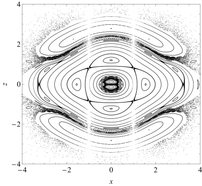
(a) Global portrait

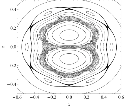
(b) Magnification of the central region

Figure 1: Poincaré cross sections of the system (1.1) for $a=b=c=0$, on the surface $y=0$

(a) Time series

(b) Two-dimensional phase portrait

Figure 2: Stable periodic motion of the system (1.1) for the parameters: $a=b=c=0$, with the initial condition: $(x_{0},y_{0},z_{0})=(0,0,2.21)$

(a) Time series

(b) Two-dimensional phase portrait

Figure 3: Quasi periodic motion of the system (1.1) for the parameters: $a=b=c=0$, with the initial condition: $(x_{0},y_{0},z_{0})=(0,0,1.6)$

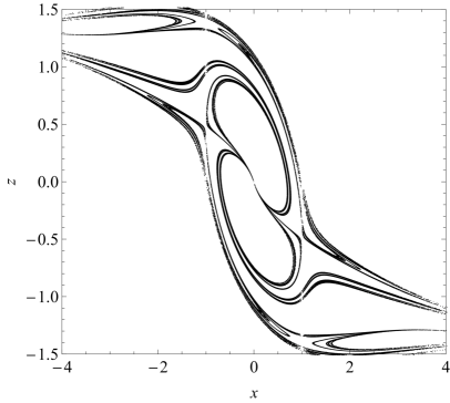
(a) Parameters: $a=1,b=0.001,c=0.8$

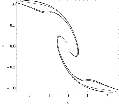
(b) Parameters: $a=1,b=0.1,c=0.95$

Figure 4: Poincaré cross sections of the system (1.1) on the surface $y=1.5$

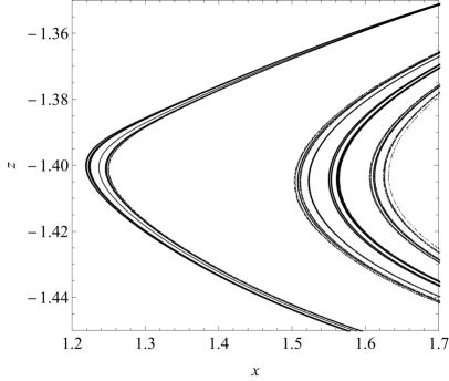
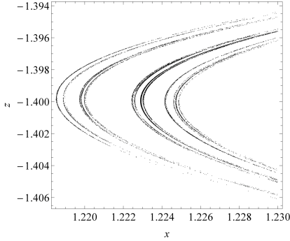
Figure 5: Magnification of the right bottom region of Fig. 4(a) showing fractals structure.

In Figuers 1 and 4 we show such sections. They were generated for certain values of parameters $(a,b,c)$. The cross-section planes are specified as $y=0$ and $y=1.5$, respectively. The coordinates on these planes are $(x,z)$. Figure 1 presents first section and the magnification around its centre. Surprisingly, even for zeroth values of the parameters, the system reveals very rich dynamics. We can detect three types of motion: periodic, quasi-periodic and chaotic, see Figs. 2 and 3 presenting periodic and quasi periodic solutions. In fact the Poincaré section visible in Figure 1 is similar to those for conservative systems. Whereas Figure 4 posses totally different structure. For chosen values of parameters given in captions in Figure 4, we obtain shapely elegant strange attractors of the fractal structure, i.e., their posses the hidden layers structure preserving self-similarity, see Figure 5 showing magnifications of the right-bottom region of the Figure 4(a).

The complex behaviour of this model apparent from the Poincaré cross sections as well as previously mentioned methods and techniques, suggests its non-integrability. But these numerical signs of non-integrability were obtained only for chosen values of parameters. The high sensitivity of chaotic systems to change the initial conditions makes it impossible to predict the effects of economic decisions in the long time scale. Therefore, it is crucial to ask whether there exists any set of values of parameters for which this system is integrable. It is very important question from the economical point of view to avoid undesirable trajectories and make the precise economic prediction possible. However, it is technically impossible to make the numerical analysis for all values of parameters. For finding integrable cases one needs a strong tool to distinguish values of parameters for which the system is suspected to be integrable.

2 Integrability analysis

For Hamiltonian systems for which we have a precise notion of integrability, i.e., integrability in the Liouville sense, there are many approaches to the integrability studies: Hamilton-Jacobi theory, normal forms, perturbation theory, splitting of separateness and recently, the Morales–Ramis theory based on the differential Galois approach. Whereas for non-Hamiltonian systems there is no so many approaches. It is due to the fact that for non-Hamiltonian systems there is no a commonly accepted definition of the integrability Thus, we should first specify what, in the considered context, the integrability means.

Definition 1.

For a given $n$-dimensional system

$$\dot{\boldsymbol{x}}=\boldsymbol{v}(\boldsymbol{x}),\qquad\boldsymbol{x}=(x_{1},\dots,x_{n})^{T}\in\mathbb{C}^{n},$$ (2.1)

by B-integrability we understand the existence of $1\leq k\leq n$ functionally independent first integrals $F_{1},\dots,F_{k}$, and $n-k$ symmetries, i.e., vector fields $\boldsymbol{w}_{1}(\boldsymbol{x})=\boldsymbol{v}(\boldsymbol{x}),\dots,\boldsymbol{w}_{n-k}(\boldsymbol{x})$ such that

$$[\boldsymbol{w}_{i},\boldsymbol{w}_{j}]=0,\quad\text{and}\quad\boldsymbol{w}_{j}[F_{i}]=0,\quad\text{for}\quad 1\leq i\leq k,\quad 1\leq j\leq n-k.$$ (2.2)

Then we say that the system is integrable by quadrature.

In this definition, the second condition means that functions $F_{1},\dots,F_{k}$ are common first integrals of vector fields $\boldsymbol{w}_{1},\dots,\boldsymbol{w}_{n-k}$. It can be shown that if a system (2.1) is B-integrable, then it is integrable by quadrature. That is, all its solutions can be obtained by means of finite sequence of algebraic operations and calculations of primitive functions.

The aim of this letter is to check whether there exist any set of values of parameters $(a,b,c)$ for which the system (1.1) is integrable. The main result is formulated in the following theorem.

Theorem 2.1.

Huang–Li nonlinear financial model (1.1) is not B-integrable in the class of meromorphic functions of variables $(x,y,z)$ for all real values of parameters $(a,b,c)$.

To prove this theorem we investigate variational equations along a particular solution and we study their differential Galois group. This approach of finding necessary conditions for integrability in a framework of differential Galois theory was mostly used in the context of Hamiltonian systems. It is described by Morales–Ramis theory. Thanks to this approach many new integrable cases were detected, see e.g., [24, 25, 18, 19]. For a general introduction to differential Galois theory as well as Morales–Ramis theory please consult the papers [26, 21, 17]. Although the system (1.1) is not a Hamiltonian, some parts of of the described differential Galois approach to its integrability study can be adopted. The key implication is following. If a system (1.1) has functionally independent meromorphic first integral, then the differential Galois group of variational equations along a particular non-equilibrium solution has a rational invariant. The first applications of the differential Galois theory to non-Hamiltonian systems the interested reader can find in [16, 23].

Originally, the Morales–Ramis theory was formulated for Hamiltonian systems for which we identify integrability as the integrability the Liouville sense. However, if we restrict ourself to B-integrability, then we have a elegant generalization of this theory. Namely, with the system (2.1) we can also consider its cotangent lift, i.e., a Hamiltonian system defined in $\mathbb{C}^{2n}$ with the following Hamiltonian function

$$H=\sum_{i=1}^{n}p_{i}v_{i}(\boldsymbol{x}),$$ (2.3)

where $\boldsymbol{x}=(x_{1},\dots,x_{n})$ and $\boldsymbol{p}=(p_{1},\dots,p_{2})$ are canonical coordinates defined in a symplectic manifold $M=\mathbb{C}^{2n}$. In a recent paper [1] Ayoul and Zung shown that if the original system (2.1) is integrable, then the lifted system generated by the function (2.3) is integrable in the Liouville sense. Hence, for both Hamiltonian and non-Hamiltonian systems, we have the same necessary integrability condition, i.e., the identity component of the differential Galois group of variational equations must be Abelian. We summarize the above facts by the following theorem that gives necessary integrability conditions for non-Hamiltonian systems.

Theorem 2.2.

(Ayoul–Zung) Assume that the system (2.1) is meromorphically B-integrable, then the identity component of the differential Galois group of variational equations along a particular non-equlibrium solution is Abelian.

2.1 Proof of Theorem 2.1

The system (1.1) possess the invariant manifold

$${\mathscr{N}}=\left\{(x,y,z)\in\mathbb{C}^{3}|x=z=0\right\}.$$ (2.4)

Indeed, equations (1.1) restricted to ${\mathscr{N}}$ read

$$\dot{x}=0,\quad\dot{y}=1-by,\quad\dot{z}=0.$$ (2.5)

Hence solving this equations, we obtain our particular solution $\boldsymbol{\varphi}(t)=(0,y(t),0)$. Let $\boldsymbol{X}=[X,Y,Z]^{T}$ denotes the variations of $\boldsymbol{x}=[x,y,z]^{T}$, then the first order variational equations along $\boldsymbol{\varphi}(t)$ take the form

$$\begin{split}&\frac{\mathrm{d}\phantom{t}}{\mathrm{d}\mspace{1.0mu}t}\boldsymbol{X}=\boldsymbol{A}(t)\boldsymbol{X},\quad\boldsymbol{A}(t)=\dfrac{\partial\boldsymbol{v}(\boldsymbol{x})}{\partial\boldsymbol{x}}(\boldsymbol{\varphi}(t)),\end{split}$$ (2.6)

where the matrix $\boldsymbol{A}(t)$ is given by

$$\boldsymbol{A}(t)=\begin{bmatrix}y-a&0&1\\ 0&-b&0\\ -1&0&-c\\ \end{bmatrix}.$$

Since the particular solution corresponds to a motion along $y$-axis, the equations for $X$ and $Z$ form a subsystem of the normal variational equations that can be rewritten as a one second order differential equation

$$\ddot{X}+(a-c-y)\dot{X}+\left(ac+(b-c)y\right)X=0.$$ (2.7)

Next, by means of the change of the independent variable

$$t\longrightarrow z=\frac{-1+by(t)}{b^{2}},$$ (2.8)

and using chain formulae for transformation of derivatives

$$\frac{\mathrm{d}\phantom{t}}{\mathrm{d}\mspace{1.0mu}t}=\dot{z}\frac{\mathrm{d}\phantom{z}}{\mathrm{d}z},\quad\frac{\mathrm{d}^{2}\phantom{t}}{\mathrm{d}t^{2}}=\dot{z}^{2}\frac{\mathrm{d}^{2}\phantom{z}}{\mathrm{d}z^{2}}+\ddot{z}\frac{\mathrm{d}\phantom{z}}{\mathrm{d}z},$$

we can rewrite equation (2.7) as

$$X^{\prime\prime}+p(z)X^{\prime}+q(z)X=0,$$ (2.9)

where prime denotes derivatives with respect to $z$. The explicit form of the coefficients $p(z)$ and $q(z)$ are the following

$$p(z)=1+\frac{1+b(b-a-c)}{b^{2}z},\quad q(z)=\frac{b-c+abc}{b^{3}z^{2}}+\frac{b-c}{bz}.$$ (2.10)

The classical change of the dependent variable

$$X=w\exp\left[-\frac{1}{2}\int_{z_{0}}^{z}p(s)\mathrm{d}s\right],$$ (2.11)

transforms (2.9) into its reduced form

$$w^{\prime\prime}(z)-r(z)w=0,\qquad r(z)=\frac{1}{2}p^{\prime}(z)+\frac{1}{4}p(z)^{2}-q(z),$$ (2.12)

with coefficient $r(z)$

$$r(z)=\frac{1}{4}-\frac{d+b^{2}}{2b^{2}z}+\frac{d^{2}-b^{4}-4b^{2}}{4b^{4}z^{2}},$$ (2.13)

where

$$d:=ab-bc-1.$$ (2.14)

In equation (2.12) with the coefficient $r(z)$ given above we immediately recognize the Whittaker equation

$$w^{\prime\prime}(z)-\left(\frac{1}{4}-\frac{\kappa}{z}+\frac{4\mu^{2}-1}{4z^{2}}\right)w(z)=0,$$ (2.15)

with

$$\kappa:=\frac{d+b^{2}}{2b^{2}},\quad\mu:=\frac{\sqrt{d^{2}-4b^{2}}}{2b^{2}}.$$ (2.16)

This equation has one regular singularity at $z=0$ and one irregular at $z=\infty$.

Here we should underline one significant fact. Namely, the respective transformations (2.8) and (2.11) change in general a whole differential Galois group of variational equations (2.6). However, the clue is that they do not affect to the identity component of the group, see e.g., [21]. Thus, according to the Theorem 2.2, in order to prove a non-integrability of our original nonlinear system (1.1) it is enough to show that the identity component of the differential Galois group ${\mathcal{G}}$ of variational equations (2.6) and thus its rationalized-reduced form (2.12) is not Abelian. Necessary conditions for abelianity of the identity component of the differential Galois group of the Whittaker equation are the following.

Theorem 2.3.

The identity component of the Galois group of the Whittaker equation (2.15) is Abelian if and only if the numbers $(p,q)$ defined by

$$p:=\kappa+\mu-\frac{1}{2},\qquad q:=\kappa-\mu-\frac{1}{2}$$ (2.17)

belong to $(\mathbb{N}\times-\mathbb{N}^{*})\cup(-\mathbb{N}^{*}\times\mathbb{N})$.

For details see Subsection 2.8.3 given in [21]. According to this theorem the numbers $(p,q)$ are integer such that one of them is positive and other negative. Thus, its product $pq$ should be always negative. In our case, however, it is easy to verify that this condition cannot be satisfied. Namely, for $(\kappa,\mu)$ given in (2.16), we obtain the following equality

$$pq=\kappa^{2}-\kappa-\mu^{2}+\frac{1}{4}=\frac{1}{b^{2}},$$ (2.18)

which cannot be fulfilled for $b\geq 0$. This ends the proof.

3 Conclusions

Although the obstructions to integrability obtained by means of analysis of differential Galois group of variational equations are one of the strongest known, the frequent obstacle in its applications is finding a particular non-equilibrium solution for a given dynamical system. Even though it is a some limitation, it is weaker than many of the assumptions required in other methods and the result of application of this method is a non-integrability proof of the considered system finally ending its analysis. Furthermore, if the system depends on certain parameters (e.g. masses, parameters describing the forces acting on the system), then usually we can prove its non-integrability for almost all values of parameters except some finite set of values. In this way the new integrable cases can be found. We shown the application of this approach on the example of intensively studied nonlinear financial model (1.1). We proved that this particular system is not integrable in the class of functions meromorphic in variables $(x,y,z)$ for all values of parameters $(a,b,c)$. However, it seems that many others different economical and financial models are waiting for such kind of analysis. It is an open problem.

References

- [1] M. Ayoul and N. T. Zung. Galoisian obstructions to non-Hamiltonian integrability. C. R. Math. Acad. Sci. Paris, 348(23-24):1323–1326, 2010.
- [2] W. J. Baumol and J. Banhabib. Chaos: Significance, mechanism, and economic applications. Journal of Economic Perspectives, 3(1):77–105, 1989.
- [3] W. C. Chen. Dynamics and control of a financial system with time-delayed feedbacks. Chaos, Solitons Fractals, 37(4):1198 – 1207, 2008.
- [4] A. C.-L. Chian. Nonlinear dynamics and chaos in macroeconomics. International Journal of Theoretical and Applied Finance, 03(03):601–601, 2000.
- [5] A. C.-L. Chian, F. A. Borotto, E. L. Rempel, and C. Rogers. Attractor merging crisis in chaotic business cycles. Chaos, Solitons Fractals, 24(3):869 – 875, 2005.
- [6] L. De Cesare and M. Sportelli. A dynamic IS-LM model with delayed taxation revenues. Chaos Solitons Fractals, 25(1):233–244, 2005.
- [7] L. Fanti and P. Manfredi. Chaotic business cycles and fiscal policy: an IS-LM model with distributed tax collection lags. Chaos Solitons Fractals, 32(2):736–744, 2007.
- [8] Q. Gao and J. Ma. Chaos and Hopf bifurcation of a finance system. Nonlinear Dynam., 58(1-2):209–216, 2009.
- [9] D. Huang and H. Li. Theory and method of the nonlinear economics. Sichuan Univ. Press: Chengdu, 1993.
- [10] A. Jabbari and H. Kheiri. Anti-synchronization of a modified three-dimensional chaotic finance system with uncertain parameters via adaptive control. Int. J. Nonlinear Sci., 14(2):178–185, 2012.
- [11] U. E. Kocamaz, A. Göksu, H. Taskin, and Y. Uyaroglu. Isynchronization of chaos in nonlinear finance system by means of sliding mode and passive control methods: A comparative study. ITC, 44:172–181, 2015.
- [12] H.-W. Lorenz. Nonlinear dynamical economics and chaotic motion. Springer-Verlag, Berlin, second edition, 1993.
- [13] H.-W. Lorenz and H. E. Nusse. Chaotic attractors, chazotic saddles, and fractal basin boundaries: Goodwin’s nonlinear accelerator model reconsidered. Chaos Solitons Fractals, 13(5):957–965, 2002.
- [14] J. Ma and Y. Chen. Study for the bifurcation topological structure and the global complicated character of a kind of nonlinear finance system. I. Appl. Math. Mech., 22(11):1119–1128, 2001.
- [15] J. Ma and Y. Chen. Study for the bifurcation topological structure and the global complicated character of a kind of nonlinear finance system. II. Appl. Math. Mech., 22(12):1236–1242, 2001.
- [16] A. J. Maciejewski and M. Przybylska. Non-integrability of {ABC} flow. Physics Letters A, 303(4):265 – 272, 2002.
- [17] A. J. Maciejewski and M. Przybylska. Differential galois theory and integrability. Int. J. Geom. Methods Mod. Phys., 6(8):1357–1390, 2009.
- [18] A. J. Maciejewski and M. Przybylska. Integrability of Hamiltonian systems with algebraic potentials. Physics Letters A, 380(1-2):76 – 82, 2016.
- [19] A. J. Maciejewski, W. Szumiński, and M. Przybylska. Note on integrability of certain homogeneous Hamiltonian systems in 2D constant curvature spaces. 2016. arXiv:1606.01084 [nlin.SI], in print.
- [20] R. M. May and J. R. Beddington. Nonlinear difference equations: Stable points, stable cycles, chaos. Unpublished manuscript, 1975.
- [21] J. J. Morales-Ruiz. Differential Galois theory and non-integrability of Hamiltonian systems. Progress in Mathematics, Birkhauser Verlag, Basel, 1999.
- [22] G. Orlando. A discrete mathematical model for chaotic dynamics in economics: Kaldora’s model on business cycle. Mathematics and Computers in Simulation, 125:83 – 98, 2016.
- [23] M. Przybylska. Differential galois obstructions for integrability of homogeneous newton equations. J. Math. Phys, 49(2):022701–1–022701–40, 2008.
- [24] O. Pujol, J. P. Pérez, J. P. Ramis, C. Simó, S. Simon, and J. A. Weil. Swinging Atwood machine: experimental and numerical results, and a theoretical study. Phys. D, 239(12):1067–1081, 2010.
- [25] W. Szumiński, A. J. Maciejewski, and M. Przybylska. Note on integrability of certain homogeneous Hamiltonian systems. Phys. Lett. A, 379(45-46):2970–2976, 2015.
- [26] M. Van der Put and M. F. Singer. Galois theory of linear differential equations. Springer-Verlag, Berlin, 2003.
- [27] M. Yang and G. Cai. Chaos control of a non-linear finance system. Journal of Uncertain Systems, 5(4):263–270, 2011.
- [28] H. Yu, G. Cai, and Y. Li. Dynamic analysis and control of a new hyperchaotic finance system. Nonlinear Dynam., 67(3):2171–2182, 2012.
- [29] X. Zhao, Z. Li, and S. Li. Synchronization of a chaotic finance system. Appl. Math. Comput., 217(13):6031–6039, 2011.
- [30] W. Zhou, L. Pan, Z. Li, and W. A. Halang. Non-linear feedback control of a novel chaotic system. International Journal of Control, Automation and Systems, 7(6):939, 2009.