Anyonic self-induced disorder in a stabilizer code:
quasi-many body localization in a translational invariant model

Abstract

We enquire into the quasi-many-body localization in topologically ordered states of matter, revolving around the case of Kitaev toric code on the ladder geometry, where different types of anyonic defects carry different masses induced by environmental errors. Our study verifies that the presence of anyons generates a complex energy landscape solely through braiding statistics, which suffices to suppress the diffusion of defects in such clean, multi-component anyonic liquid. This non-ergodic dynamics suggests a promising scenario for investigation of quasi-many-body localization. Computing standard diagnostics evidences that a typical initial inhomogeneity of anyons gives birth to a glassy dynamics with an exponentially diverging time scale of the full relaxation. Our results unveil how self-generated disorder ameliorates the vulnerability of topological order away from equilibrium. This setting provides a new platform which paves the way toward impeding logical errors by self-localization of anyons in a generic, high energy state, originated exclusively in their exotic statistics.

Many-body localization (MBL) Gornyi et al. (2005); Basko et al. (2006); Oganesyan and Huse (2007); Pal and Huse (2010); Bauer and Nayak (2013); Imbrie (2016) generalizes the concept of single particle localization Anderson (1958) to isolated interacting systems, where many-body eigenstates in the presence of sufficiently strong disorder can be localized in a region of Hilbert space even at nonzero temperature. An MBL system comes along with universal characteristic properties such as area-law entanglement of highly excited states (HES) Bauer and Nayak (2013); Kjäll et al. (2014), power-law decay and revival of local observables Serbyn et al. (2014a, b), logarithmic growth of entanglement Žnidarič et al. (2008); Bardarson et al. (2012); Vosk and Altman (2013); Serbyn et al. (2013a) as well as the violation of “eigenstates thermalization hypothesis” (ETH) Deutsch (1991); Srednicki (1994); Rigol et al. (2008). The latter raises the appealing prospect of protecting quantum order as well as storing and manipulating coherent information in out-of-equilibrium many-body states Huse et al. (2013); Chandran et al. (2014); Bahri et al. (2015); Potter and Vishwanath (2015); Yao et al. (2015).

Recently it has been questioned Carleo G (2011); De Roeck and Huveneers (2014); De Roeck and Huveneers (2014); Hickey et al. (2016); Schiulaz and Müller (2014); Schiulaz et al. (2015); Papić et al. (2015); Yao et al. (2016); Barbiero et al. (2015); Smith et al. (2017) whether quench disorder is essential to trigger ergodicity breaking or one might observe glassy dynamics in translationally invariant systems, too. In such models initial random arrangement of particles effectively fosters strong tendency toward self-localization characterized by MBL-like entanglement dynamics, exponentially slow relaxation of a typical initial inhomogeneity and arrival of inevitable thermalization. This asymptotic MBL–tagged quasi-MBL Yao et al. (2016)–in contrast to the genuine ones, is not necessarily accompanied by the emergence of infinite number of conserved quantities Serbyn et al. (2013b); Huse et al. (2014); Chandran et al. (2015); Ros et al. (2015).

Here we present a novel mechanism toward quasi-MBL in a family of clean self-correcting memories, in particular the Kitaev toric code Dennis et al. (2002); Kitaev (2003) on ladder geometry, a.k.a. the Kitaev ladder (KL) Karimipour (2009); Langari et al. (2015). The elementary excitations of KL are associated with point-like quasi-particles, known as electric (e) and magnetic (m) charges. Our main interest has its roots in the role of non-trivial statistics between anyons that naturally live in (highly) excited states of such models.

Stable topological memories, by definition, need to preserve the coherence of encoded quantum state for macroscopic timescales. However, due to their thermal fragility Castelnovo and Chamon (2007, 2008); Brown et al. (2016); Nussinov and Ortiz (2008); Hastings (2011), specially far-from-equilibrium Kay (2009); Zeng et al. (2016), the problem of identifying a stable low-dimensional quantum memory is still unsecure. One of the major obstacles to this end is that they do not withstand dynamic effects of perturbations whenever a nonzero density of anyons are initially present in the system. Indeed, propagation of even one pair of deconfined anyons around non-contractible loops of the system leads to logical error. In addition, system’s dynamics under generic perturbations could be so tangled that the quantum memory equilibrates in the thermal Gibbs state, in which no topological order survives Hastings (2011).

So far, extensive searches have been carried out to combat the mentioned shortcomings  Chamon (2005); Kim and Haah (2016); Alicki et al. (2010); Mazáč and Hamma (2012); Brown et al. (2014); Hamma et al. (2009); Pedrocchi et al. (2013); Landon-Cardinal et al. (2015); Tsomokos et al. (2011); Wootton and Pachos (2011); Stark et al. (2011). In particular, exerting an external disorder on a stabilizer code strengthens the stability of topological phase Tsomokos et al. (2011) and ensures the single particle localization of Abelian anyons as long as their initial density is below a critical value Wootton and Pachos (2011); Stark et al. (2011). The inquiry is whether one can treat the fragility of translationally invariant, topologically ordered systems in the presence of an arbitrary initial density of anyons living in HES.

We supply clear-cut evidences that random configurations of anyons in HES of KL prompts a self-generated disorder purely due to the mutual braiding statistics. Performing a dual mapping suggests that nonzero density of the magnetic charges, as barriers, poses a kinetic constraint on dynamics of the electric ones and hinders the propagation of the confined charges on non-trivial class of loops around the cylindrical surface of KL. Subsequently, it is more favorable for the initial information to be encoded in sub-spaces with higher density of anyons! Finally, we provide numerical evidences that the effective disorder leads to the existence of an exponentially diverging time scale for dynamical persistence of the initial inhomogeneity, along with an intermediate slow growth of the entanglement entropy, all of which are essential qualities of quasi-MBL.

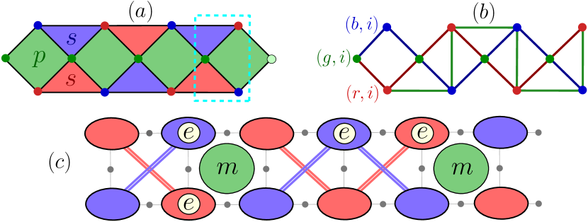
Figure 1: (a) KL with periodic-boundary condition in leg and open-boundary condition along rungs. Spin-1/2 particles are placed on the $3L$ nodes of the lattice. (b) Multiplying $Z$ operators along the red (blue) line yields dual spin $\mu^{x}_{r/b,i}$, and a similar string of $X$ operators along the green line defines $\mu^{x}_{g,i}$. (c) The pictorial demonstration of the dual KL Hamiltonian, Eq. (6), for $t_{m}=0$.

Kitaev ladder Hamiltonian.—KL is composed of $L$ unit cells, each with three sites, that we will refer to as red, green, and blue sites (see Fig. 1-(a)), and spin-1/2 particles are placed on the $N=3L$ nodes of the lattice. The unperturbed Hamiltonian is defined by $L$ plaquette stabilizer, ${B}_{p}$, and $2L$ vertex stabilizer terms on the triangles of the ladder, $A_{s}^{r/b}$, as follow:

$$H^{KL}_{0}\leavevmode\nobreak\ \leavevmode\nobreak\ \leavevmode\nobreak\ =-j_{m}\sum_{i}B_{p}(i)-j_{e}\sum_{i}\left(A_{s}^{r}(i)+A_{s}^{b}(i)\right),$$ (1)

$$B_{p}(i)\leavevmode\nobreak\ \leavevmode\nobreak\ =Z_{g,i}Z_{r,i}Z_{b,i}Z_{g,i+1},$$ (2)

$$A_{s}^{r/b}(i) =X_{r/b,i-1}X_{g,i}X_{b/r,i},$$

where $X_{i}$ and $Z_{i}$ are the x- and z-component of Pauli operators, respectively. We set $j_{e}$, $j_{m}>0$ and choose an overall energy scale by setting $j_{e}=1$. KL can be viewed as the Kitaev toric code with surface termination along the rungs direction (a.k.a. surface code Dennis et al. (2002)) whose width is one. This model represents $\mathbb{Z}_{2}\times\mathbb{Z}_{2}$ symmetry-protected topological (SPT) order associated to anyonic parities Langari et al. (2015); sup .

Now we would like to perturb the KL Hamiltonian such that $e$ (charge) and $m$ (flux), corresponding to $A_{s}=-1$ and $B_{p}=-1$, respectively, hop across the ladder and gain kinetic energy. To this end we consider the perturbed KL with the generic Ising terms:

$$H^{KL}=H_{0}^{KL}-t_{e}\sum_{\langle i,j\rangle\in\partial p}Z_{i}Z_{j}-t_{m}\sum_{i\in legs}X_{i}X_{i+1},$$ (3)

where $t_{e}$ ($t_{m}$) is the hopping strength of $e$ ($m$). Via applying $Z_{g,i}Z_{r,i}$, which commutes with every plaquette and star operator except $A_{s}^{r}(i)$ and $A_{s}^{r}(i+1)$, an $e$ charge on site $(r,i)$ transfers to $(r,i+1)$. We could also use $Z_{b,i}Z_{g,i+1}$ to carry out the same task. However, $Z_{b,i}Z_{g,i+1}=B_{p}(i)Z_{g,i}Z_{r,i}$, and therefore the total contribution to the Hamiltonian is $(1+B_{p}(i))Z_{g,i}Z_{r,i}$. That being so, the Ising interactions are coupled to the dynamical $\mathbb{Z}_{2}$ gauge field and the hopping of an $e$ charge from $(r,i)$ to $(r,i+1)$ depends on the value of $B_{p}(i)=(-1)^{n^{m}_{i}}$, which takes into account the parity of $m$ anyon on site $(g,i)$, or equivalently, the mutual braiding statistics of $e$ and $m$. Hence, the hopping of $e$ is blocked if there is a flux on its way. Likewise, $X_{r,i}X_{b,i+1}$ transports one unit of $m$ charge from plaquette $(g,i)$ to $(g,i+1)$ and vice versa. We could also consider $X_{b,i}X_{r,i+1}$ to reach the same goal. However, $X_{b,i}X_{r,i+1}=A_{s}^{r}(i+1)A_{s}^{b}(i+1)X_{r,i}X_{b,i+1}$, and again the movement of $m$ is intertwined with the density of $e$’s along its way.

Unlike the single particle studies in the presence of disorder Wootton and Pachos (2011); Stark et al. (2011), in a many-body picture, the transport properties of Abelian anyons might strongly be affected by their exotic statistics, so that $e$ and $m$ as two distinct quasi-particles are able to mutually suppress their own dynamics, even in a clean system. The latter property is the characteristic feature of Falicov-Kimball like Hamiltonians whose non-ergodic dynamics has been recently investigated as a candidate for disorder-free localization Schiulaz and Müller (2014); Schiulaz et al. (2015); Papić et al. (2015); Yao et al. (2016); Barbiero et al. (2015); Smith et al. (2017).

To directly reveal this hidden structure, we introduce a non-local dual transformation, which maps Eq. 3 to three coupled transverse field Ising (TFI) chains (see Fig. 1-(b)),

$$H^{KL}_{\rm dual}\leavevmode\nobreak\ =\leavevmode\nobreak\ -\sum_{i}\left(j_{m}\mu_{g,i}^{z}+t_{m}\mu_{g,i}^{x}\mu_{g,i+1}^{x}(1+\mu_{r,i+1}^{z}\mu_{b,i+1}^{z})\right)$$ (6)

$$-\sum_{i}\left(j_{e}\mu_{b,i}^{z}+t_{e}\mu_{b,i}^{x}\mu_{b,i+1}^{x}(1+\mu_{g,i}^{z})\right)$$

$$-\sum_{i}\left(j_{e}\mu_{r,i}^{z}+t_{e}\mu_{r,i}^{x}\mu_{r,i+1}^{x}(1+\mu_{g,i}^{z})\right),$$

where

$$\mu_{g,i}^{x}=\prod_{j\geq i}X_{r,j}X_{b,j+1},\quad\mu_{r/b,i}^{x}=\prod_{j\geq i}Z_{g,j}Z_{r/b,j},$$

and $\mu_{g,i}^{z}=B_{p}(i)$, $\mu_{r/b,i}^{z}=A_{s}^{r/b}(i)$. This model features glassy dynamics for the $\mu_{g,r/b}$ degrees of freedom, associated to the anyonic excitations of the KL. For example, in the non-interacting limit $t_{m}=0$ an effective description of $H^{KL}_{\rm dual}$ reduces to two TFI chains coupled to the static $\mathbb{Z}_{2}$ gauge field, $\mu^{z}_{g}$. These gauge degrees of freedom form a set of $L$ constants of motion with trivial dynamics. Hence, an arbitrary initial nonzero density of fluxes $\rho_{m}$ energetically suppresses charges’ kinetic interactions (see Fig.1-(c)). Indeed, a typical initial inhomogeneity of $\{\mu_{g}\}=\pm 1$ is dynamically manifested in a self-generated disorder potential, $t^{\prime}_{e}(i)=t_{e}(1+\mu_{g,i})$, with the dilution distribution,

$$\mathcal{P}(t^{\prime}_{e})=(1-\rho_{m})\delta(t^{\prime}_{e}-2t_{e})+\rho_{m}\delta(t^{\prime}_{e}),$$ (7)

where for a fixed value of $\rho_{m}$, different configurations of fluxes correspond to different realizations of disorder. In such situation, dynamics of the whole system will be identical to that of two decoupled, disordered TFI chains in terms of $\hat{\mu}_{r/b}$, which are Anderson localized Stinchcombe (1981).

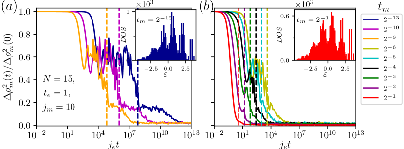
Figure 2: Relaxation of the flux inhomogeneity density for $N=15$ (spins) with fixed $t_{e}=1$ and varying $t_{m}$, averaged over $150$ random initial states $\lvert\psi_{N_{m}}\rangle$, with $N_{m}=3$ in the (a) fast and (b) slow dynamics regime. Vertical dashed lines represent time at $\tau_{eff}$. (insets) DOS for the cases with largest and smallest mass ratio $t_{m}/t_{e}$.

Anyonic self-localization and quasi-MBL regime.—The outlined glassy blueprint is inspiring to look for the counterpart of quasi-MBL Yao et al. (2016) in an Abelian many-body system. In analogy to the observed quasi-MBL in a trivial admixture of heavy and light particles Schiulaz and Müller (2014); Schiulaz et al. (2015); Papić et al. (2015); Yao et al. (2016); Barbiero et al. (2015), one needs to choose the mass ratio of the quasi-particles to be large enough, as long as the “isolated bands” Papić et al. (2015) due to finite-size effects is not manifested. In the KL, $t_{e}$ ($t_{m}$) controls the strength of the effective disorder (interaction) as well as the effective mass of $e$ ($m$) anyons com . Thus, we consider the limit $0<t_{m}\ll t_{e}$, where $m$’s have a large but finite effective mass. Now we initialize the whole system in a typical inhomogeneous configuration $\lvert\psi_{N_{m}}\rangle$ of $N_{m}=\rho_{m}L$ fluxes, which are selected near the middle of the spectrum of $H^{KL}$. Then, we compute the evolution of the flux inhomogeneity density under $H^{KL}$,

$$\Delta\rho_{m}^{2}(t)\equiv\dfrac{1}{L}\sum^{L}_{p=1}\lvert\langle\psi_{N_{m}}\rvert(n^{m}_{p+1}(t)-n^{m}_{p}(t))\lvert\psi_{N_{m}}\rangle\rvert^{2},$$ (8)

which vanishes for any perfect delocalized state. As illustrated in Fig. 2-(a,b), for $t_{m}\gtrsim 0.01$ fast relaxation of the initial inhomogeneity due to resonance admixtures Schiulaz and Müller (2014); Schiulaz et al. (2015) takes place within the time scale $\tau_{int}\sim t_{m}^{-1}$, while in the opposite limit, i.e. small $t_{m}$, the initial inhomogeneity plateau persists until $\tau_{int}$. Moreover, the residual inhomogeneity remains even at later times $\tau_{eff}\sim t_{e}/t_{m}^{2}$. Subsequent to this time, the collective slow dynamics eventually gives way to complete relaxation at $\tau_{R}$. As discussed in Papić et al. (2015), to ensure the robustness of the numerical results against finite-size effects, the density of states (DOS) must not display any isolated classical bands, which can be clearly seen in the insets of Fig. 2.

To gain further insights on the nature of the three distinct time scales that characterize the relaxation dynamics of anyons, $\tau_{int}<\tau_{eff}\leq\tau_{R}$, we have also looked at the growth of entanglement entropy $S_{ent}=-\rho_{A}\ln\rho_{A}$ for half-system $A$ with strong disorder $t_{e}=10$ (see Fig. 3-(a)). Prior to $\tau_{int}$, charges perceive the fluxes as if they are immobile barriers. Hence, after an initial growth, $S_{ent}$ saturates to the first plateau, conveying the single particle localization length of charges. Subsequent to $\tau_{int}$ hybridization of fluxes arrives, which in turn intertwines with the charge dynamics. Thus, the entropy shows logarithmic growth until the finite-size dephasing of charges wins at the second plateau. At $\tau_{eff}$, the dephasing of the fluxes sets in and the entanglement grows even more slowly to saturate eventually at $\tau_{R}$.

It is worth mentioning that the same time scales also determine the evolution of the quantity $\mathcal{I}(\tau)\!=$$\frac{\overline{\Delta\rho_{m}^{2}(\tau)}-\overline{\Delta\rho_{m}^{2}(\infty)}}{\overline{\Delta\rho_{m}^{2}(0)}-\overline{\Delta\rho_{m}^{2}(\infty)}}$, where $\overline{\Delta\rho_{m}^{2}(\tau)}\equiv{\tau^{-1}}\int_{0}^{\tau}dt\leavevmode\nobreak\ {\Delta\rho_{m}^{2}(t)}$ (see Fig. 3-(a)). Moreover, the late time behavior of $\mathcal{I}(\tau)$ signifies that the full relaxation eventually occurs but at very long times. This anyonic slow dynamics is in contrast to true MBL in which an initial inhomogeneity never completely decays. These results resemble those characteristic behaviors observed in the previous proposal of quasi-MBL Yao et al. (2016).

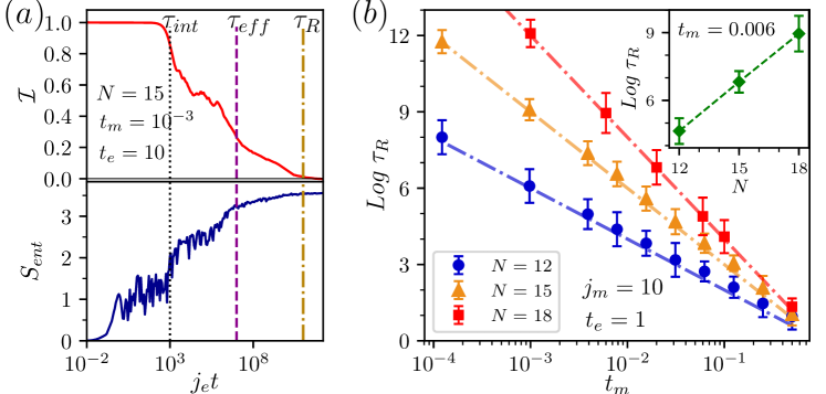
Figure 3: (a) Upper panel: Relaxation of the time averaged inhomogeneity of fluxes for $N=15$ and $t_{e}=10$, in quasi-MBL regime at $t_{m}=10^{-3}$, averaged over $150$ initial states with $N_{m}=3$. Lower panel: entanglement dynamics for subsystem of size $N_{A}=8$, averaged over $250$ random product states. (b) The scaling behavior of $\tau_{R}$ versus $t_{m}$ at fixed $t_{e}=1$, for $N=12,15,18$ with the initial total number of fluxes, $N_{m}=2,3,4$, respectively. The dot-dashed lines denote the analytical estimation $\tau_{R}t_{m}\propto(t_{e}/t_{m})^{N_{m}-1}$. (inset) The expected exponentially diverging behavior of $\tau_{R}$ with system sizes at $t_{m}=0.006$ in the quasi-MBL regime.

Following the perturbative argument presented in Schiulaz and Müller (2014), the final decay time of initial inhomogeneity should display scaling behavior as $\tau_{R}t_{m}\propto(t_{e}/t_{m})^{N_{m}-1}$ in KL. To confirm this parametric dependence, we plot numerically extracted value of $\tau_{R}$ versus $t_{m}$ in Fig. 2-(b) sup for different system sizes at fixed value of $t_{e}=1$. Our numerical results not only illustrate a good agreement with the rough estimation presented above, but also imply the exponential dependence of $\tau_{R}$ on the system size with growing number of fluxes in the quasi-MBL regime.

Lastly, we would like to address whether the fast relaxation in such anyonic liquids is followed by the viability of ETH. In this respect, we discard the pair creation/annihilation of fluxes, which might happen as a result of $X_{r,i}X_{b,i+1}$ terms in Eq. (3). Typically, this recombination processes are less likely for the heavy particles in comparison with the light ones. Therefore, it is a reasonable assumption to consider $\tilde{H}_{KL}=\hat{P}_{N_{m}}H^{KL}\hat{P}_{N_{m}}$, where $\hat{P}_{N_{m}}$ is the projection operator into the subspace with fixed $N_{m}$ sup .

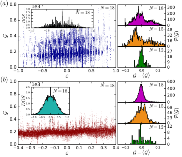
Figure 4: (a) Failing of ETH for the case $(t_{e},t_{m})=(1,0.001)$. Left panel: The exception value of $\mathcal{G}$ in momentum eigenstates versus energy density. Inset displays DOS for $\tilde{H}_{KL}$. Right panel: $\mathcal{P}(\mathcal{G})$ for all eigenstates in the energy window $\varepsilon\in[-0.09,0.09]$ in the middle of the energy band for different system sizes. The average value is removed from the distribution for visibility. (b) Manifestation of ETH for $(t_{e},t_{m})=(1,0.5)$. $\mathcal{P}(\mathcal{G})$ is plotted in the interval $\varepsilon\in(0,0.15]$. Results are reported for $(N,N_{m})=(12,2)$, $(15,3)$ and $(18,3)$.

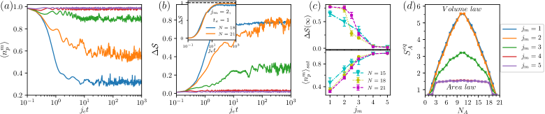
Figure 5: (a) Evolution of the expectation value of $\hat{n}^{m}_{p}$ by varying the flux mass gap $j_{m}$, for $N=21$, $t_{e}=10$, $t_{m}=0.6$ and the pre-quench state initialized in $\rho_{m}=1$ and $\rho_{e}=0$. Since both the Hamiltonian and initial state are translationally invariant, the results for all plaquettes are the same. (b) The information spreading, (c) late time saturation values and (d) scaling of $S_{ent}$ with different subsystem sizes $N_{A}$, at $j_{e}t=10^{3}$, where $\langle n_{p}^{m}\rangle$ saturates to its long-time value. (inset) The heating procedure in the ergodic phase, in which systems with sizes $N=18$ and $21$ could approach their thermal Gibbs state.

We evaluate $\mathcal{G}\equiv\langle n_{p}^{m}n_{p+1}^{m}\rangle$ in the simultaneous eigenstates of $\tilde{H}_{KL}$ and momentum, and collect the results from all momenta. Fig. 4-(a) quantifies $\mathcal{G}$ in different energy densities, for $(t_{e},t_{m})=(1,0.001)$. In the whole energy intervals, the value of $\mathcal{G}$ is spread considerably in a wide range. On top of that, the distribution function $\mathcal{P}(\mathcal{G})$ near the middle of the band has a very broad half-width and peaks at different values as the system size is increased (right panel in Fig. 4-(a)) indicating a strong non-ergodic behavior. For the fast dynamics, e.g. $(t_{e},t_{m})=(1,0.5)$, the system rather obeys ETH prediction: DOS becomes continuous, $\mathcal{P}(\mathcal{G})$ sharply picked around its mean value and the width of the distribution decreases by increasing the system size, as illustrated in Fig. 4-(b). Hence, whenever $t_{e}$ and $t_{m}$ are in the same order of magnitude, the fast relaxation occurs along with the validity of ETH in HES.

Resilience of the topological order following a quench.—To further inspect the fingerprints of the emergent kinetic constraint in Eq. 6 on non-equilibrium anyonic dynamics, we proceed with the scenario of the quantum quench. We initially prepare the system in $\lvert\phi_{0}\rangle=(1/2)\leavevmode\nobreak\ (1+\hat{W}_{x})\lvert\{n_{p}^{m}\},\{n_{s}^{e}\}\rangle$, where $\hat{W}_{x}$ is one of the two logical operators that encode the topological qubit, and $\lvert\{n_{p}^{m}\},\{n_{s}^{e}\}\rangle$ is an exact eigenvector of $H^{KL}_{0}$ including a specific pattern of $e$’s and $m$’s (with $\rho_{m}$ ($\rho_{e}$) density of $m$ ($e$) preparatory anyons). According to the SPT nature of $H^{KL}_{0}$ sup , the corresponding eigenstates are short-range entangled, and thus cold state. We are specially interested in those transitionally invariant pre-quench states with $\rho_{m}=1$ and $\rho_{e}=0$, wherein initial information is encoded in the sub-space with maximum number of $m$ anyons. By performing massively parallel time integration based on Chebyshev expansion Balay et al. (2016, 1997); Hernandez et al. (2005) to evolve system under $H^{KL}$, we measure the spreading of the stored initial information as well as the non-equilibrium heating procedure over the course of time,

$$\Delta\mathcal{S}=\dfrac{S_{ent}(t)-S_{0}}{S_{page}-S_{0}},$$ (9)

where $S_{ent}(t)$, $S_{0}$ and $S_{page}$ are bipartite entanglement entropies associated with $\lvert\phi(t)\rangle$, $\lvert\phi_{0}\rangle$ and an infinite temperature state Page (1993), respectively.

For $t_{m}=0$, it follows from Eq. 7 that the dynamical effect of perturbation would be completely suppressed due to the presence of fluxes in each plaquette. Indeed, regardless of the magnitude of $j_{m}$ and $t_{e}$, the spreading of information is strictly impeded, even in the absence of any explicit form of disorder in either the Hamiltonian or the initial state! This result is comparable to Ref. Smith et al., 2017, where non-ergodic dynamics is induced solely through the presence of static gauge degrees of freedom, albeit through a distinct mechanism.

For $t_{m}\neq 0$ thermalization process can be controlled by the flux mass gap $j_{m}$ Dennis et al. (2002). In this respect, to build up the tendency toward the survival of preparatory fluxes in the system we increase $j_{m}$ (see Figs. 5-(a,c)). As a result, the thermalization process slows down at a continually growing rate (see Figs. 5-(b,c)). Hence, scaling of $S_{ent}$ with different subsystem sizes $N_{A}$ reforms from volume law to area law, as depicted in Fig. 5-(d). An approximate area law is observed for $j_{m}\gtrsim 4$, while for $j_{m}=1$, $2$ the scaling obeys volume law foo . Notably, the system with sizes considered here, in the thermal regime, reaches its infinite temperature state (see inset of Fig. 5-(b)), which is never observed in those suffering from finite-size effects.

Discussion.—We identified the anyonic self-localization as an emergent property purely rooted in the intrinsic statistics of the Abelian anyons and extended the so-called quasi-MBL picture to self-correcting quantum codes. This provides a novel mechanism distinct by nature from the recent proposals on disorder-free localization  Schiulaz and Müller (2014); Schiulaz et al. (2015); Yao et al. (2016); Grover and Fisher (2014); Smith et al. (2017).

As mentioned earlier, a number of approaches have been proposed to remedy the thermal fragility of the quantum memories with $D<4$, such as: considering clean cubic Chamon (2005); Kim and Haah (2016) and higher dimensional codes Alicki et al. (2010); Mazáč and Hamma (2012) with a more complex structure than the toric one, 2D codes consisting of N-level spins Brown et al. (2014), coupling 2D codes to a massless scalar field Hamma et al. (2009); Pedrocchi et al. (2013); Landon-Cardinal et al. (2015) as well as employing Anderson localization machinery Tsomokos et al. (2011); Wootton and Pachos (2011); Stark et al. (2011). Our results on anyonic self-induced disorder indicate that an exponentially glassy dynamics could be induced even (i) in a low-dimensional, clean, and simple-structure models, and remarkably (ii) this glassiness is enhanced by increasing either the density of errors and/or environmental perturbations Schiulaz et al. (2015); sup .

The scenario discussed in this work could be easily generalized sup to 2D quantum double models such as the Levin-Wen model Levin and Wen (2005). As little progress has been made toward investigation of MBL in topologically ordered 2D systems, our study breaks the ground for future researches.

A closely related concept to quasi-MBL in multi-component systems is quantum disentangled liquid Grover and Fisher (2014); Garrison et al. (2017); Veness et al. (2016), wherein “post-measurement” of the anyon configuration is identical to the error syndrome; that is, the first step in the error-correcting protocol. It is tempting to see whether such measurement procedure on a topological state supports this claim. Intuitively, could there a quantum disentangled spin liquid be found?

Acknowledgements.—We highly appreciate fruitful discussions and neat comments by Fabien Alet, Moeen Najafi-Ivaki, Mazdak Mohseni-Rajaee and Arijeet Pal. The authors would like to thank Sharif University of Technology for financial supports and CPU time from Cosmo cluster. AV was supported by the Gordon and Betty Moore Foundation’s EPiQS Initiative through Grant GBMF4302.

Kitaev Ladder (KL).—We first briefly discuss the main properties of the KL Hamiltonian, $H_{0}^{KL}$, in (highly) excited states to give an insight on its nature as an anyonic liquid. In KL periodic-boundary condition in the leg direction leads to the global constraint $\prod_{i}A_{s}^{r/b}(i)=\mathbb{1}$, which ensures that (i) any energy level in the whole spectrum will have at least twofold degeneracy and (ii) $2L-1$ independent charge degrees of freedom are created/annihilated in pairs. However, fluxes can be created/annihilated singly in contrast to the 2D toric code on torus. One can also define the occupation operators of charges and fluxes as $\hat{n}_{i}^{e}=(1-A_{s}^{r/b}(i))/2$ and $\hat{n}_{i}^{m}=(1-B_{p}(i))/2$, respectively. In term of occupation operators, $H_{0}^{KL}$ simply counts the total number of e and m anyons in the system. The basis which diagonalizes $H_{0}^{KL}$ has the following closed form in the occupation number representation:

$$\lvert\{n_{i}^{m}\},\{r_{i}\}\rangle=\hat{P}_{\{n_{i}^{m}\}}\hat{g}_{\{r_{i}\}}\lvert x+\rangle^{\otimes N},\quad$$ (S1)

where $\hat{P}_{\{n_{i}^{m}\}}=\prod_{i}(1+(-1)^{n_{i}^{m}}B_{p}(i))/2$, $\hat{g}_{\{r_{i}\}}=\prod_{\begin{subarray}{c}i\in\text{D}\end{subarray}}Z_{i}^{r_{i}}$ and $\lvert x+\rangle$ is the eigenstate of $X$, i.e. $X\lvert x+\rangle=\lvert x+\rangle$. $\hat{g}_{\{r_{i}\}}$ is a member of the Abelian group $G$ (consisting of $2^{2L}$ different set of configurations, $\{r_{i}=0,1\}$), which performs all spin-flip operations for $2L$ spins placed on the global path $D$ (see Fig. S1). By the action of $G$ on the charge vacuum state, one can generate all $2^{2L-1}$ different independent charge configurations. $\hat{P}_{\{n_{i}^{m}\}}$ is the projection operator to the subspace with flux configuration, $\{n_{i}^{m}\}$, where $2^{L}$ different set of $\{n_{i}^{m}=0,1\}$ can generate corresponding flux degrees of freedom. However, $\{r_{i}=1;\;\forall i\}$ is a special case for which $W_{z}\equiv\hat{g}_{\{r_{i}=1\}}$ goes over the whole system on homologically nontrivial path $D$. Accordingly, for any state $\rvert\{n_{i}^{m}\},\{r_{i}\}\rangle$, there is a degenerate state,

$$\lvert\{n_{i}^{m}\},\{\overline{r}_{i}\}\rangle=\hat{W}_{z}|\{n_{i}^{m}\},\{r_{i}\}\rangle,\quad\hat{W}_{z}=\prod_{\begin{subarray}{c}i\in\text{$D$}\end{subarray}}Z_{i},$$ (S2)

where $\hat{W}_{z}$ plays the role of Wilson loop, which creates a pair of charges on a vertex, rounds them across the system, and then annihilates them. This process is accompanied by changing topological sector of states (associated to different eigenstates of logical operator $\hat{W}_{x}=\prod_{\begin{subarray}{c}i\in\text{$D^{\prime}$}\end{subarray}}X_{i}$) and can be interpreted as diffusion of unchecked errors across the ladder after a time proportional to the system size, a.k.a. logical error. Hence, generating glassy dynamics in highly-excited states (HES) of such disorder-free stabilizer codes impedes the mentioned procedure and puts forward a new paradigm for realizing more stable quantum memories at finite temperature, the task which assigned to the quasi many-body localization (qMBL) mechanism through this work.

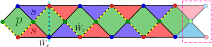
Figure S1: KL as a surface code terminated in one direction. Dashed lines indicate topologically nontrivial path $D$ and $D^{\prime}$.

as mentioned in the main text, the ground state of KL model (with twofold degeneracy in the free charge and flux sectors $\{n_{i}^{m}=0,r_{i}=0;\;\forall\leavevmode\nobreak\ i\}$) can not be smoothly connected to a short range entangled state without breaking the following Ising symmetries, explicitly or spontaneously:

$$\mathcal{P}_{m}=\prod_{i=1}^{L}B_{p}(i)\leavevmode\nobreak\ ,\quad\mathcal{P}_{e}=\prod_{s}{A_{s}^{r}(i)}=\prod_{s}{A_{s}^{b}(i)}.$$ (S3)

The action of these symmetries on occupation number basis Eq. (S1) can be interpreted as anyonic parity, such that $\mathcal{P}_{m}$ shows the flux parity and $\mathcal{P}_{e}$ represents the charge parity in the red or blue vertices.

Boundary condition for the dual pseudo-spins.—In this section, we study the effect of the flux parity, defined in Eq. (S3), on determining the boundary condition (BC) for pseudo-spins $\mu_{r/b}$. Because of the global constraint $\prod_{i}\mu_{r,i}^{z}\mu_{b,i}^{z}=\mathbb{1}$, $\mu_{r/b}$’s describe only $2L-1$ independent degrees of freedom. That being so, applying dual transformation on the original spins of the KL with periodic-BC results a 1-to-2 mapping between $\mu_{r/b}$’s and original spins. One can consider two additional independent ancillary degrees of freedom, in the virtual $(L+1)$-th unit cell of the ladder (see Fig. S1). According to our definition for blue and red pseudo-spins, $\mu_{r/b,i}^{x}=\prod_{j\geq i}Z_{g,j}Z_{r/b,j}$, the x-component of ancillary pseudo-spins are product over an empty set, hence $\mu_{r,L+1}^{x}=\mu_{b,L+1}^{x}=1$. On the other hand, the string operators $\mu_{r,1}^{x}$ and $\mu_{b,1}^{x}$ are two special cases that commute with $H^{KL}$ and in terms of the original spins take the form $\mu_{r,1}^{x}=W_{z}$, $\mu_{b,1}^{x}=\mathcal{P}_{m}W_{z}$. Combination of these properties gives:

$$1=\mu_{r,L+1}^{x}=\left\{\begin{array}[]{ll}\mu_{r,1}^{x}&\mbox{if $\;\;W_{z}=+1$}\\ -\mu_{r,1}^{x}&\mbox{if $\;\;W_{z}=-1$}.\end{array}\right.$$ (S4)

In fact, $\mu_{r,1}^{x}$ and $\mu_{b,1}^{x}$ are dynamical variables that are not independent from each other and determine the BCs on the $\mu$’s. So, according to Eq. (S4), the flux parity

$$\mathcal{P}_{m}=\mu_{r,1}^{x}\mu_{b,1}^{x}\equiv(-1)^{N_{m}}=\left\{\begin{array}[]{ll}+1\\ -1,\end{array}\right.$$ (S7)

determines the BC of the red and blue TFI chains in $H^{KL}_{\rm dual}$ and relates them to each other in such a way that for the even parity two chains simultaneously have periodic-BC or antiperiodic-BC, but for the odd parity one chain has periodic-BC while another must have antiperiodic-BC and vice versa. In fact, the mentioned BCs, by doubling the size of the Hilbert space, establish a one-to-one mapping between all energy levels of $H^{KL}_{\rm dual}$ and the perturbed KL Hamiltonian.

Numerical methods for extracting the complete relaxation time.—The numerical data presented in Fig. 3-(b) of the main text, have been extracted as follow: For $N=12$ and $15$, we performed extensive exact diagonalization and averaged over $150$ random initial configurations of magnetic charges with fixed total number of fluxes, $N_{m}$. For $N=18$ –due to lack of special symmetries, e.g. $U(1)$, that can significantly decrease the effective Hilbert space dimension–, we implemented another advanced methods: (i) In the fast relaxation regime ($t_{m}\sim t_{e}$), we use massively parallel time integration method Balay et al. (2016, 1997); Hernandez et al. (2005) based on Chebyshev expansion that is suitable for simulating the dynamics up to the moderate times ($j_{e}t\sim 10^{4}$) that are much larger than the typical value of $\tau_{R}$ in this regime. (ii) In order to compute $\tau_{R}$ for slow relaxation regime we simulate relaxation time trace via shift-and-invert Lanczos method, which has been employed in the previous study of quasi-MBL Yao et al. (2016). To find a large portion of spectrum, we use the implementation of PETSc Balay et al. (2016, 1997) and SLEPc Hernandez et al. (2005) rely on MUMPS Amestoy et al. (2006) to perform parallel sparse Cholesky factorization as a direct solver. To check the accuracy of extracted $\tau_{R}$, we progressively increase the number of targeted eigenstates from $100$ to $5500$, which indicates the convergence of $\tau_{R}$ to its analytical estimation $\tau_{R}t_{m}\propto(t_{e}/t_{m})^{N_{m}-1}$. We also considered different targeted energy densities, centered at $j_{e}/2$ and $j_{e}/4$, which does not show any quantitative difference. The reported results are averaged over $600$ realizations of initial states and extracted data from targeted energy densities centered at $j_{e}/2$ and $j_{e}/4$.

Projected Hamiltonian.—As mentioned in the main text, dynamics of the fluxes in our model is governed by the two-body ferromagnetic Ising interaction, $X_{i}X_{j}$ between the nearest neighbor spins, that sit on the legs of the ladder. Here, we would like to restrict our study to the effect of flux dynamics on localization or thermalization of finite energy states, therefore we discard the creation/annihilation of fluxes which might occurs as a result of $X_{i}X_{j}$ terms. Typically, this recombination processes are less likely for the heavy particles in comparison with the light ones, equivalent to the condition $j_{m}\gg t_{e}>t_{m}$.

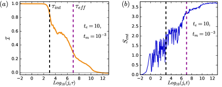
Figure S2: (a) Relaxation of flux inhomogeneity and (b) Growth of entanglement entropy for subsystem cut at $8$-th spin, corresponding to strong effective disorder governed by $\tilde{H}_{KL}$ for $(N,\,N_{m})=(15,\,3)$, averaged over 200 random product states.

Here, we impose this restriction by projecting the leg-Ising interaction onto the subspace with a fixed total number of flux by $\hat{P}_{N_{m}}=\sum^{{}^{\prime}}_{\{n_{i}^{m}\}}\hat{P}_{\{n_{i}^{m}\}}$, where $\hat{P}_{\{n_{i}^{m}\}}$ is defined in Eq. (S1), and the summation is restricted to those configurations in which $N_{m}=\sum_{i}n_{i}^{m}$ is fixed. In this respect, the projected Hamiltonian is given by $\tilde{H}_{KL}=\hat{P}_{N_{m}}H^{KL}\hat{P}_{N_{m}}$. The matrix elements of $\tilde{H}_{KL}$ can only connect different configurations of the flux anyons with fixed $N_{m}$. Since the total number of fluxes, in addition to the flux parity, will be a constant of motion of $\tilde{H}_{KL}$, using this projected Hamiltonian is more efficient for computational purposes. In this situation, the effective mass of heavy particles living in finite energy levels is inversely controlled by $t_{m}$ in each fixed flux sector, $j_{m}$ is an irrelevant parameter. To check the validity of this approach, in Fig. S2 we compute entanglement dynamics and relaxation of the initial inhomogeneity governed by $\tilde{H}_{KL}$, which shows the same qualitative behavior in comparison to those governed by $H^{KL}$ presented in the main text.

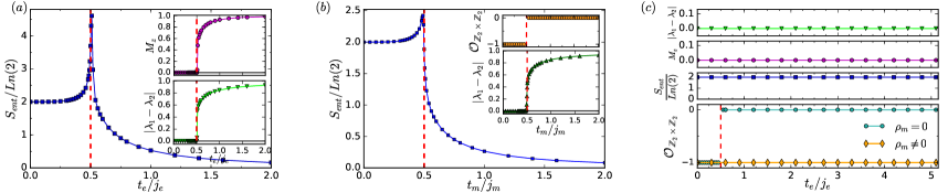
Figure S3: (a) von-Neumann entropy $S_{ent}$, calculated by an implementation of iTEBD method with $\chi=64$ for $H^{KL}(t_{m}=0)$ in $\rho_{m}=0$ sector. The upper and bottom insets show magnetization, $M_{z}$, and the gap between two largest Schmidt coefficients $|\lambda_{1}-\lambda_{2}|$, respectively. All data shows diverging behavior at $t_{e}^{c}=j_{e}/2$. (b) von-Neumann entropy computed for $H^{KL}(t_{e}=0)$ in $\rho_{e}=0$ sector. The upper and bottom insets show $\mathcal{O}_{\mathbb{Z}_{2}\times\mathbb{Z}_{2}}$ defined in Eq. (S8) and gap between two largest Schmidt coefficients, respectively. (c) The three top panels display the effect of nonzero density of fluxes on the same quantities plotted in (a). The lowest panel specifies the phase factor order parameter ,$\mathcal{O}_{\mathbb{Z}_{2}\times\mathbb{Z}_{2}}$, which reveals robustness of the SPT order for $\rho_{m}\neq 0$.

Robustness of SPT phase in finite flux density.—To reveal the effect of nonzero flux density on robustness of the SPT order, we consider $H^{KL}_{\rm dual}$ with $t_{m}=0$. First, in $\rho_{m}=0$ the dual Hamiltonian reduces to two decoupled clean TFI chains. Accordingly, the system has a well-known phase transition at $t^{c}_{e}=j_{e}/2$. The paramagnetic phase for $t_{e}<j_{e}/2$ in the $\mu_{r/b}$-picture is identical to the $\mathbb{Z}_{2}\times\mathbb{Z}_{2}$ SPT phase in the language of the original model Langari et al. (2015), while $t_{e}>j_{e}/2$ is smoothly connected to the $j_{e}=0$ fixed point and represents the trivial polarized phase. However, for $\rho_{m}>0$ the TFI chains are no longer clean and effectively experience a random dilution disorder. According to the the exact solution presented in Ref. Stinchcombe, 1981, for arbitrary (increasing) values of $t_{e}$, even an infinitesimal $\rho_{m}$ spoils any long range magnetic order. For this reason, in the $\mu_{r/b}$-picture system is always in the paramagnetic phase, and thus the existence of m-errors favors the topological order.

Numerical approach.—We employed infinite time-evolving block decimation (iTEBD) algorithm Orús and Vidal (2008), which is based on infinite matrix-product state (iMPS) representation to numerically check the validity of above analytical results. In the original model, for the case of $\rho_{m}=0$, we compute the half-cut von-Neumann entanglement entropy, $S_{ent}=-tr(\rho_{L/2}\ln\rho_{L/2})$, where $\rho$ is the ground state density matrix. The main plot of Fig. S3-(a) shows a diverging behavior of $S_{ent}$ at $t_{e}^{c}=j_{e}/2$. Moreover, the magnetization, $M_{z}=\sum_{i}Z_{i}/N$ (presented in the upper inset of Fig. S3-(a)), shows a transition from a non-magnetic phase for $t_{e}<j_{e}/2$ to a spontaneously symmetry breaking phase for $t_{e}>j_{e}/2$. The lower inset of Fig. S3-(a) unveils the difference between the two largest magnitudes of Schmidt coefficients, $|\lambda_{1}-\lambda_{2}|$, where the degeneracy of $\lambda_{1}$ and $\lambda_{2}$ for $t_{e}<j_{e}/2$ is the characteristic feature of SPT phase Pollmann et al. (2010). A similar behavior holds in the case $H^{KL}(t_{e}=0)$ in the $\rho_{e}=0$ sector, where the phase transition occurs at $t_{m}^{c}=j_{m}/2$ (see Fig S3-(b)). Additionally, we compute the phase factor order parameter Pollmann and Turner (2012):

$$\mathcal{O}_{\mathbb{Z}_{2}\times\mathbb{Z}_{2}}=\left\{\begin{array}[]{ll}0&\mbox{if $|\eta_{z}|<1$ or $|\eta_{x}|<1$ }\\ \dfrac{1}{\chi}tr(U_{z}U_{x}U_{z}^{\dagger}U_{x}^{\dagger})&\mbox{if $|\eta_{z}|<1=|\eta_{x}|=1$,}\end{array}\right.$$ (S8)

where $\eta_{z}$ and $\eta_{x}$ are the largest eigenvalues of the generalized transfer matrix Pollmann and Turner (2012) constructed by symmetry operators $\mathcal{P}_{m}$ and $\mathcal{P}_{e}$, respectively, and $U_{z}^{\dagger}$ and $U_{x}^{\dagger}$ are eigenvectors corresponding to them (here $\chi$ is the bond dimension of iMPS). The symmetry protected nontrivial phase, symmetry-breaking phase and symmetry protected trivial phase are characterized by $\mathcal{O}_{\mathbb{Z}_{2}\times\mathbb{Z}_{2}}=\{-1,0,1\}$, respectively. The behavior of the mentioned quantities implies that for $t_{e}<j_{e}/2$ ($t_{m}<j_{m}/2$) the perturbed system at zero flux sector (zero charge sector) belongs to the $\mathbb{Z}_{2}\times\mathbb{Z}_{2}$ quantum spin liquid phase.

Now, we consider the parent Hamiltonian $H_{0}^{{}^{\prime}KL}$, which is different from $H_{0}^{KL}$ in that, we set $j_{m}\rightarrow j^{{}^{\prime}}_{m}=-j_{m}$. The ground state of $H_{0}^{{}^{\prime}KL}$ is in the full flux sector equivalent to the highest energy sector of $H_{0}^{KL}$. It can be shown that after adding the plaquette-Ising interaction (as charge kinetic term) to the $H_{0}^{{}^{\prime}KL}$, the ground state of perturbed parent Hamiltonian, $H^{{}^{\prime}}_{KL}$, remains in $\rho_{m}\neq 0$ sectors, provided that the rough estimate $t_{e}\lesssim j_{m}/2$ holds. It is worth mentioning that iTEBD algorithm does not guarantee the final wavefunction of $H^{{}^{\prime}}_{KL}$ to remain in a sector with finite flux density for arbitrary enhancing value of $t_{e}$. Hence, mentioned constraint ensures that the zero-flux sector is not reachable as $t_{e}$ is increased.

The results of our numerical simulation for $H^{{}^{\prime}}_{KL}$ with $j^{{}^{\prime}}_{m}=-10j_{e}$ are presented in Fig. S3-(c), which shows no evidence for a quantum phase transition at $\rho_{m}\neq 0$. The von-Neumann entropy is $2\ln 2$, where magnetization is zero, the Schmidt coefficients are degenerate and $\mathcal{O}_{\mathbb{Z}_{2}\times\mathbb{Z}_{2}}=-1$. All these results indicate the robustness of SPT order as a consequence of self-generated disorder. This effect is also comparable with Ref. Tsomokos et al., 2011, in which the external random field with dilution distribution stabilizes intrinsic topological order against arbitrarily strong magnetic fields.

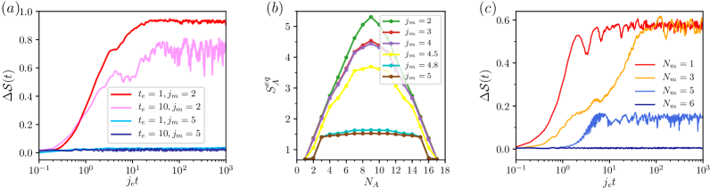
Figure S4: (a) Spreading of the information for pre-quench state initialized in $\rho_{m}=1$, $t_{m}=0.6$ and $N=18$. (b) Scaling of $S_{ent}$ with different subsystem sizes for $t_{e}=1$, $t_{m}=0.6$ and $\rho_{m}=1$. (c) The effect of initial flux density on spreading of information for $t_{e}=10$, $t_{m}=0.3$ and $j_{m}=5$.

The role of interaction and effective temperature in the quenching procedure.—Here, we investigate the dependence of the non-ergodic quench behavior on the interaction and effective temperature. Apart from the parameters $j_{m}$ and $t_{m}$, the flux density in pre-quench state and $t_{e}$ can be seen as additional controlling parameters for initial energy density (trough the relation $\varepsilon_{\rho_{m}}=-j_{m}(1-\rho_{m})-2j_{e}$) and the strength of the effective disorder, respectively. By reducing the strength of interaction from $t_{e}=10$ (see Fig. 5 in the main text) to $t_{e}=1$, the information spreading escalates as shown in Fig. S4-(a). Subsequently, as shown in Fig. S4-(b), the scaling of entanglement changes behavior from area law to volume law, approximately around $j_{m}=4.5$, which become greater than $j_{m}\sim 3$ for $t_{e}=10$. Moreover, lowering the number of initial fluxes in the pre-quench state results in an upsurge in the heating process, in the way that the Ising perturbations adversely redesign the initial short-range state to a mixed one (see Fig. S4-(c)). As a result, increasing the effective temperature and strength of interaction ameliorates the resilience of topological order as well as robustness of the initial encoded information.

Generalization to other SPT phases.—We would like to present a more general picture on the implications of topological order and braiding statistics for the self-localization of anyon excitations in highly excited states. In quantum double models such as Levin-Wen model or Kitaev’s toric code, an anyon of type $a$ can be transported from site $i$ to site $j$ along the directed path $\gamma$ connecting the two sites through applying open string operators (Wilson line operators) of type $a$, $W^{a}_{\gamma}$. In order to mobilize anyons in the system and let them acquire kinetic energy, we can add $\sum_{a}\sum_{\gamma}g^{a}_{\gamma}W^{a}_{\gamma}$ to the ideal (exactly solvable) Hamiltonian, where $g^{a}_{\gamma}$ is the amplitude of path $\gamma$. Now, imagine two distinct paths $\gamma_{1}$ and $\gamma_{2}$. The product of the two open string operators along $\gamma_{1}$ and $\overline{\gamma_{2}}$ ($\gamma_{2}$ with opposite direction), i.e. $W_{c}\equiv W^{a}_{\gamma_{1}}W^{a}_{\overline{\gamma_{2}}}=W^{a}_{\gamma_{1}}\left(W^{a}_{\gamma_{2}}\right)^{-1}$, forms a closed string (Wilson loop operator). The resulting loop can take various quantized values depending on the total anyon charge inside path $\gamma_{3}\equiv\gamma_{1}\overline{\gamma_{2}}$. Now suppose the resulting path, i.e. $\gamma_{3}$, encloses total anyon charge equal to $b$. The Wilson operator $W_{c}$ measures the braid statistics between anyons $a$ and $b$ and is independent of path $\gamma_{3}$ (as far as it encompasses the anyon charge $b$). Therefore, $W^{a}_{\gamma_{2}}=W_{c}W^{a}_{\gamma_{1}}$. As a result, the total contribution of the two paths $\gamma_{1}$ and $\gamma_{2}$ is $\left(g^{a}_{\gamma_{1}}+g^{a}_{\gamma_{2}}W_{c}\right)W^{a}_{\gamma_{1}}$. Now, let us assume the two paths $\gamma_{1}$ and $\gamma_{2}$ are related via some symmetry operations, for instance the mirror symmetry with respect to the $x$ axis. In that case, we must choose $\left|g^{a}_{\gamma_{1}}\right|=\left|g^{a}_{\gamma_{2}}\right|$ if we want to preserve that symmetry. Since, $W_{c}$ depends on the total anyon charge trapped inside loop $\gamma_{3}$ and it may take a different value upon the translation of $\gamma_{3}$, the perturbations can be viewed as disordered anyon hopping terms where the disorder is due to the nontrivial anyon braid statistics as discussed previously.

References

- Gornyi et al. (2005) I. V. Gornyi, A. D. Mirlin, and D. G. Polyakov, Phys. Rev. Lett. 95, 206603 (2005).
- Basko et al. (2006) D. Basko, I. Aleiner, and B. Altshuler, Annals of Physics 321, 1126 (2006).
- Oganesyan and Huse (2007) V. Oganesyan and D. A. Huse, Phys. Rev. B 75, 155111 (2007).
- Pal and Huse (2010) A. Pal and D. A. Huse, Phys. Rev. B 82, 174411 (2010).
- Bauer and Nayak (2013) B. Bauer and C. Nayak, Journal of Statistical Mechanics: Theory and Experiment 2013, P09005 (2013).
- Imbrie (2016) J. Z. Imbrie, Journal of Statistical Physics 163, 998 (2016).
- Anderson (1958) P. W. Anderson, Phys. Rev. 109, 1492 (1958).
- Kjäll et al. (2014) J. A. Kjäll, J. H. Bardarson, and F. Pollmann, Phys. Rev. Lett. 113, 107204 (2014).
- Serbyn et al. (2014a) M. Serbyn, Z. Papić, and D. A. Abanin, Phys. Rev. B 90, 174302 (2014a).
- Serbyn et al. (2014b) M. Serbyn, M. Knap, S. Gopalakrishnan, Z. Papić, N. Y. Yao, C. R. Laumann, D. A. Abanin, M. D. Lukin, and E. A. Demler, Phys. Rev. Lett. 113, 147204 (2014b).
- Žnidarič et al. (2008) M. Žnidarič, T. c. v. Prosen, and P. Prelovšek, Phys. Rev. B 77, 064426 (2008).
- Bardarson et al. (2012) J. H. Bardarson, F. Pollmann, and J. E. Moore, Phys. Rev. Lett. 109, 017202 (2012).
- Vosk and Altman (2013) R. Vosk and E. Altman, Phys. Rev. Lett. 110, 067204 (2013).
- Serbyn et al. (2013a) M. Serbyn, Z. Papić, and D. A. Abanin, Phys. Rev. Lett. 110, 260601 (2013a).
- Deutsch (1991) J. M. Deutsch, Phys. Rev. A 43, 2046 (1991).
- Srednicki (1994) M. Srednicki, Phys. Rev. E 50, 888 (1994).
- Rigol et al. (2008) M. Rigol, V. Dunjko, and M. Olshanii, Nature 452, 854 (2008).
- Huse et al. (2013) D. A. Huse, R. Nandkishore, V. Oganesyan, A. Pal, and S. L. Sondhi, Phys. Rev. B 88, 014206 (2013).
- Chandran et al. (2014) A. Chandran, V. Khemani, C. R. Laumann, and S. L. Sondhi, Phys. Rev. B 89, 144201 (2014).
- Bahri et al. (2015) Y. Bahri, R. Vosk, E. Altman, and A. Vishwanath, Nature Communications 6, 7341 (2015).
- Potter and Vishwanath (2015) A. C. Potter and A. Vishwanath, ArXiv e-prints (2015), arXiv:1506.00592 [cond-mat.dis-nn] .
- Yao et al. (2015) N. Y. Yao, C. R. Laumann, and A. Vishwanath, ArXiv e-prints (2015), arXiv:1508.06995 [quant-ph] .
- Carleo G (2011) S. M. F. M. Carleo G, Becca F, Scientific Reports 2, 243 (2011).
- De Roeck and Huveneers (2014) W. De Roeck and F. Huveneers, Communications in Mathematical Physics 332, 1017–1082 (2014).
- De Roeck and Huveneers (2014) W. De Roeck and F. m. c. Huveneers, Phys. Rev. B 90, 165137 (2014).
- Hickey et al. (2016) J. M. Hickey, S. Genway, and J. P. Garrahan, Journal of Statistical Mechanics: Theory and Experiment 2016, 054047 (2016).
- Schiulaz and Müller (2014) M. Schiulaz and M. Müller, AIP Conference Proceedings 1610, 11 (2014).
- Schiulaz et al. (2015) M. Schiulaz, A. Silva, and M. Müller, Phys. Rev. B 91, 184202 (2015).
- Papić et al. (2015) Z. Papić, E. M. Stoudenmire, and D. A. Abanin, Annals of Physics 362, 714 (2015).
- Yao et al. (2016) N. Y. Yao, C. R. Laumann, J. I. Cirac, M. D. Lukin, and J. E. Moore, Phys. Rev. Lett. 117, 240601 (2016).
- Barbiero et al. (2015) L. Barbiero, C. Menotti, A. Recati, and L. Santos, Phys. Rev. B 92, 180406 (2015).
- Smith et al. (2017) A. Smith, J. Knolle, D. L. Kovrizhin, and R. Moessner, Phys. Rev. Lett. 118, 266601 (2017).
- Serbyn et al. (2013b) M. Serbyn, Z. Papić, and D. A. Abanin, Phys. Rev. Lett. 111, 127201 (2013b).
- Huse et al. (2014) D. A. Huse, R. Nandkishore, and V. Oganesyan, Phys. Rev. B 90, 174202 (2014).
- Chandran et al. (2015) A. Chandran, I. H. Kim, G. Vidal, and D. A. Abanin, Phys. Rev. B 91, 085425 (2015).
- Ros et al. (2015) V. Ros, M. Müller, and A. Scardicchio, Nuclear Physics B 891, 420 (2015).
- Dennis et al. (2002) E. Dennis, A. Kitaev, A. Landahl, and J. Preskill, Journal of Mathematical Physics 43, 4452 (2002).
- Kitaev (2003) A. Kitaev, Annals of Physics 303, 2 (2003).
- Karimipour (2009) V. Karimipour, Phys. Rev. B 79, 214435 (2009).
- Langari et al. (2015) A. Langari, A. Mohammad-Aghaei, and R. Haghshenas, Phys. Rev. B 91, 024415 (2015).
- Castelnovo and Chamon (2007) C. Castelnovo and C. Chamon, Phys. Rev. B 76, 184442 (2007).
- Castelnovo and Chamon (2008) C. Castelnovo and C. Chamon, Phys. Rev. B 77, 054433 (2008).
- Brown et al. (2016) B. J. Brown, D. Loss, J. K. Pachos, C. N. Self, and J. R. Wootton, Rev. Mod. Phys. 88, 045005 (2016).
- Nussinov and Ortiz (2008) Z. Nussinov and G. Ortiz, Phys. Rev. B 77, 064302 (2008).
- Hastings (2011) M. B. Hastings, Phys. Rev. Lett. 107, 210501 (2011).
- Kay (2009) A. Kay, Phys. Rev. Lett. 102, 070503 (2009).
- Zeng et al. (2016) Y. Zeng, A. Hamma, and H. Fan, Phys. Rev. B 94, 125104 (2016).
- Chamon (2005) C. Chamon, Phys. Rev. Lett. 94, 040402 (2005).
- Kim and Haah (2016) I. H. Kim and J. Haah, Phys. Rev. Lett. 116, 027202 (2016).
- Alicki et al. (2010) R. Alicki, M. Horodecki, P. Horodecki, and R. Horodecki, Open Systems & Information Dynamics 17, 1 (2010).
- Mazáč and Hamma (2012) D. Mazáč and A. Hamma, Annals of Physics 327, 2096 (2012).
- Brown et al. (2014) B. J. Brown, A. Al-Shimary, and J. K. Pachos, Phys. Rev. Lett. 112, 120503 (2014).
- Hamma et al. (2009) A. Hamma, C. Castelnovo, and C. Chamon, Phys. Rev. B 79, 245122 (2009).
- Pedrocchi et al. (2013) F. L. Pedrocchi, A. Hutter, J. R. Wootton, and D. Loss, Phys. Rev. A 88, 062313 (2013).
- Landon-Cardinal et al. (2015) O. Landon-Cardinal, B. Yoshida, D. Poulin, and J. Preskill, Phys. Rev. A 91, 032303 (2015).
- Tsomokos et al. (2011) D. I. Tsomokos, T. J. Osborne, and C. Castelnovo, Phys. Rev. B 83, 075124 (2011).
- Wootton and Pachos (2011) J. R. Wootton and J. K. Pachos, Phys. Rev. Lett. 107, 030503 (2011).
- Stark et al. (2011) C. Stark, L. Pollet, A. m. c. Imamoğlu, and R. Renner, Phys. Rev. Lett. 107, 030504 (2011).
- (59) See Supplementary material.
- Stinchcombe (1981) R. B. Stinchcombe, Journal of Physics C: Solid State Physics 14, L263 (1981).
- (61) Generally, in a stabilizer Hamiltonian, one deals with two concepts of mass, i.e. effective mass and mass gap. The latter is defined as energy needed for creation/anihilation of anyons and controlled by and parameters.
- Balay et al. (2016) S. Balay, S. Abhyankar, M. Adams, P. Brune, K. Buschelman, L. Dalcin, W. Gropp, B. Smith, D. Karpeyev, D. Kaushik, et al., Petsc users manual revision 3.7, Tech. Rep. (Argonne National Lab.(ANL), Argonne, IL (United States), 2016).
- Balay et al. (1997) S. Balay, W. D. Gropp, L. C. McInnes, and B. F. Smith, in Modern Software Tools in Scientific Computing, edited by E. Arge, A. M. Bruaset, and H. P. Langtangen (Birkhäuser Press, 1997) pp. 163–202.
- Hernandez et al. (2005) V. Hernandez, J. E. Roman, and V. Vidal, ACM Trans. Math. Softw. 31, 351 (2005).
- Page (1993) D. N. Page, Phys. Rev. Lett. 71, 1291 (1993).
- (66) In this setting, we investigate the translationally invariant pre-quench states and the observed non-ergodic behavior takes place even at the moderate value of .
- Grover and Fisher (2014) T. Grover and M. P. A. Fisher, Journal of Statistical Mechanics: Theory and Experiment 2014, P10010 (2014).
- Levin and Wen (2005) M. A. Levin and X.-G. Wen, Phys. Rev. B 71, 045110 (2005).
- Garrison et al. (2017) J. R. Garrison, R. V. Mishmash, and M. P. A. Fisher, Phys. Rev. B 95, 054204 (2017).
- Veness et al. (2016) T. Veness, F. H. L. Essler, and M. P. A. Fisher, ArXiv e-prints (2016), arXiv:1611.02075 [cond-mat.stat-mech] .
Supplemental Material for EPAPS

References

- Amestoy et al. (2006) P. R. Amestoy, A. Guermouche, J.-Y. L’Excellent, and S. Pralet, Parallel Computing 32, 136 (2006).
- Orús and Vidal (2008) R. Orús and G. Vidal, Phys. Rev. B 78, 155117 (2008).
- Pollmann et al. (2010) F. Pollmann, A. M. Turner, E. Berg, and M. Oshikawa, Phys. Rev. B 81, 064439 (2010).
- Pollmann and Turner (2012) F. Pollmann and A. M. Turner, Phys. Rev. B 86, 125441 (2012).