Cyclohedron and Kantorovich-Rubinstein polytopes

Cyclohedron and Kantorovich-Rubinstein polytopes

Abstract

We show that the cyclohedron (Bott-Taubes polytope) $W_{n}$ arises as the polar dual of a Kantorovich-Rubinstein polytope $KR(\rho)$, where $\rho$ is an explicitly described quasi-metric (asymmetric distance function) satisfying strict triangle inequality. From a broader perspective, this phenomenon illustrates the relationship between a nestohedron $\Delta_{\mathcal{\widehat{F}}}$ (associated to a building set $\mathcal{\widehat{F}}$) and its non-simple deformation $\Delta_{\mathcal{F}}$, where $\mathcal{F}$ is an irredundant or tight basis of $\mathcal{\widehat{F}}$ (Definition 21). Among the consequences are a new proof of a recent result of Gordon and Petrov (Arnold Math. J.  3 (2), 205–218 (2017)) about $f$-vectors of generic Kantorovich-Rubinstein polytopes and an extension of a theorem of Gelfand, Graev, and Postnikov, about triangulations of the type A, positive root polytopes.

1 Introduction

Motivated by the classic Kantorovich-Rubinstein theorem, A.M. Vershik described in [Ve3] a canonical correspondence between finite metric spaces $(X,\rho)$ and convex polytopes in the vector space $V_{0}(X)\subset\mathbb{R}^{X}$ of all signed measures on $X$ with total mass equal to $0$. More explicitly, each finite metric space $(X,\rho)$ is associated a fundamental polytope $KR(\rho)$ (Kantorovich-Rubinstein polytope) spanned by $e_{x,y}=\frac{e_{x}-e_{y}}{\rho(x,y)}$ where $\{e_{x}\}_{x\in X}$ is the canonical basis in $\mathbb{R}^{X}$.

Kantorovich-Rubinstein polytope $KR(\rho)$ can be also described as the dual of the Lipschitz polytope $Lip(\rho)$ where,

$$Lip(\rho)=\{f\in\mathbb{R}^{X}\mid(\forall x,y\in X)\,f(x)-f(y)\leqslant\rho(x,y)\},$$ (1)

and two functions $f,g\in\mathbb{R}^{X}$ are considered equal if they differ by a constant.

Vershik raised in [Ve3] a general problem of studying (classifying) finite metric spaces according to the combinatorics of their fundamental polytopes.

Gordon and Petrov in a recent paper [GP] proved a very interesting result that the $f$-vector of the Kantorovich-Rubinstein polytope $KR(\rho)$ is one and the same for all sufficiently generic metrics on $X$. They obtained this result as a byproduct of a careful combinatorial analysis of face posets of Lipschitz polytopes. The invariance of the $f$-vector of $KR(\rho)$ can be also deduced from the fact that the type A root polytope $Root_{n}:={\rm Conv}(\mathcal{A}_{n})$, where $\mathcal{A}_{n}=\{e_{i}-e_{j}\mid 1\leqslant i\neq j\leqslant n\}$, is unimodular in the sense of [$\Delta$, Definition 6.2.10] (see also the outline in Section 2.3).

Our point of departure was an experimentally observed fact that the generic $f$-vector of Gordon and Petrov coincides with the $f$-vector of (the dual of) the cyclohedron (Bott-Taubes polytope) $W_{n}$. At first sight this is an unexpected phenomenon since $W_{n}^{\circ}$ itself is not centrally symmetric and therefore cannot arise as a Kantorovich-Rubinstein polytope $KR(\rho)$ (unless $\rho$ is allowed to be a quasi-metric!).

The symmetry of a metric is a standard assumption in the usual formulations of the Kantorovich-Rubinstein theorem, see for example [Vi1, Section 1.2.]. However this condition is not necessary. (The proof of this fact is implicit in [Vi2, Section 5], see Particular Case 5.4. on page 68.) More importantly the ‘radial vertex perturbation’ (Section 2.2) of a metric may affect its symmetry, so the extension of $KR(\rho)$ to quasi-metrics may be justified both by the ‘optimal transport’ and the ‘convex polytopes’ point of view.

We prove two closely related results which both provide explanations why the cyclohedron $W_{n}$ (and its dual polytope $W_{n}^{\circ}$) appear in the context of generic Kantorovich-Rubinstein polytopes and triangulations of the type A root polytope.

In the first result (Theorem 14), we construct a map $\phi_{n}:W_{n}^{\circ}\rightarrow Root_{n}$ which is simplicial on the boundary $\partial(W_{n}^{\circ})$ and maps bijectively $\partial(W_{n}^{\circ})$ to the boundary $\partial(Root_{n})$ of the root polytope. (In particular we obtain a triangulation of $\partial(Root_{n})$ parameterized by faces of $W_{n}$.)

This construction is purely combinatorial and diagrammatic in nature. It relies on a combinatorial description of $W_{n}$ as a graph associahedron [De] and describes simplices in $\partial(W_{n}^{\circ})$ as admissible families of intervals (arcs) in the cycle graph $C_{n}$.

Theorem 14 can also be seen as an extension of a result of Gelfand, Graev, and Postnikov [GGP, Theorem 6.3.] who described a coherent triangulation of the type A, positive root polytope $Root_{n}^{+}={\rm Conv}\{e_{i}-e_{j}\mid 1\leqslant i\leqslant j\leqslant n\}$. For illustration, the standard trees depicted in [GGP, Figure 6.1.] may be interpreted as our admissible families of arcs (as exemplified in Figure 3) where all arcs are oriented from left to right.

In the second result (Theorem 31 and Proposition 34) we prove the existence and than explicitly construct a canonical quasi-metric $\rho$ such that the associated Kantorovich-Rubinstein polytope $KR(\rho)$ is a geometric realization of the polytope $W_{n}^{\circ}$.

This result has a more geometric flavor since it relies on a nestohedron representation [Po, FS] of the cyclohedron as the Minkowski sum $W_{n}=\Delta_{\mathcal{\widehat{F}}}=\sum_{F\in\mathcal{\widehat{F}}}~{}\Delta_{F}$ of simplices. In this approach the relationship between the cyclohedron $W_{n}$ and the dual $(Root_{n})^{\circ}$ of the root polytope is seen as a special case of a more general construction linking a nestohedron $\Delta_{\mathcal{\widehat{F}}}$ and its Minkowski summand $\Delta_{\mathcal{F}}$, where $\mathcal{\widehat{F}}$ is a building set and $\mathcal{F}$ its irredundant basis (Definition 21).

In Section 6 we briefly outline a different plan (suggested by a referee) for constructing quasi-metrics of “cyclohedral type”. This approach relies on the analysis of the combinatorial structure of Lipschitz polytopes for generic measures, as developed in [GP].

In ‘Concluding remarks’ (Section 7) we discuss the significance of Theorems 14 and 31. For example we demonstrate (Section 7.1) how the motivating result of Gordon and Petrov [GP, Theorem 1] can be deduced from the known results about the $f$-vectors of cyclohedra. We also offer a glimpse into potentially interesting future developments including the study of ‘tight pairs’ $(\mathcal{\widehat{F}},\mathcal{F})$ of hypergraphs (Section 7.2) and the ‘canonical quasitoric manifolds’ associated to combinatorial quasitoric pairs $(W_{n},\phi_{n})$ (Section 7.3).

2 Preliminaries

2.1 Kantorovich-Rubinstein polytopes

Let $(X,\rho)$, $|X|=n$, be a finite metric space and let $V(X):=\mathbb{R}^{X}\cong\mathbb{R}^{n}$ be the associated vector space of real valued functions (weight distributions, signed measures) on $X$. In particular, $V_{0}(X):=\{\mu\in V(X)\mid\mu(X)=0\}$ is the vector subspace of measures with total mass equal to zero, while $\Delta_{X}:=\{\mu\in V(X)\mid\mu(X)=1\wedge(\forall x\in X)\,\mu(\{x\})\geqslant 0\}$ is the simplex of probability measures.

Let $\mathcal{T}_{\rho}(\mu,\nu)$ be the cost of optimal transportation of measure $\mu$ to measure $\nu$, where the cost of transporting the unit mass from $x$ to $y$ is $\rho(x,y)$. Then [Ve1, Vi1], there exists a norm $\|\cdot\|_{KR}$ on $V_{0}(X)$ (called the Kantorovich-Rubinstein norm), such that,

$$\mathcal{T}_{\rho}(\mu,\nu)=\|\mu-\nu\|_{KR},$$

for each pair of probability measures $\mu,\nu\in\Delta_{X}$. By definition, the Kantorovich-Rubinstein polytope $KR(\rho)$, or the fundamental polytope [Ve3], associated to $(X,\rho)$, is the corresponding unit ball in $V_{0}(X)$,

$$KR(\rho)=\{x\in V_{0}(X)\mid\|x\|_{KR}\leqslant 1\}.$$ (2)

The following explicit description for $KR(\rho)$ can be deduced from the Kantorovich-Rubinstein theorem (Theorem 1.14 in [Vi1]),

$$KR(\rho)={\rm Conv}\left\{\frac{e_{x}-e_{y}}{\rho(x,y)}\mid x\in X\right\},$$ (3)

where $\{e_{x}\}_{x\in X}$ is the canonical basis in $\mathbb{R}^{X}$.

Problem 1.

(A.M. Vershik [Ve3]) Study and classify metric spaces according to combinatorial properties of their Kantorovich-Rubinstein polytopes.

2.2 Root polytopes

The convex hull of the roots of a classical root system is called a root polytope. In particular the type A root polytope, associated to the root system of type $A_{n-1}$, is the following polytope (Fig.1),

$$Root_{n}={\rm Conv}\{e_{i}-e_{j}\mid 1\leqslant i\neq j\leqslant n\}.$$ (4)

It immediately follows from (4) that the root polytope admits the following Minkowski sum decomposition,

$$Root_{n}=\Delta+\nabla=\Delta+(-\Delta)=\Delta-\Delta,$$ (5)

where $\Delta=\Delta_{n}={\rm Conv}\{e_{i}\}_{i=1}^{n}$ and $\nabla=-\Delta={\rm Conv}\{-e_{i}\}_{i=1}^{n}$.

By definition, $Root_{n}$ is the Kantorovich-Rubinstein polytope associated to the metric $\rho$ where $\rho(x,y)=1$ for each $x\neq y$. Conversely, in light of (3), each Kantorovich-Rubinstein polytope can be seen as a radial, vertex perturbation of the root polytope $Root_{n}$.

Figure 1: The boundary triangulation of $Root_{4}$ described in Theorem 14.

2.3 Unimodular triangulations and equidecomposable polytopes

A triangulation of a convex polytope $Q$ is tacitly assumed to be without new vertices. A triangulation of the boundary sphere $\partial(Q)$ of $Q$ is referred to as a boundary triangulation. Each triangulation of $Q$ produces the associated boundary triangulation (but not the other way around).

The $f$-vector of a triangulation is the $f$-vector of the associated simplicial complex. Different triangulations of either the polytope $Q$ or its boundary $\partial(Q)$ may have different face numbers, so in general the $f$-vector of a triangulation is not uniquely determined by the polytope $Q$. The simplest examples illustrating this phenomenon are the bipiramid over a triangle and the $3$-dimensional cube (the latter admits triangulations with both $5$ and $6$, three dimensional simplices).

The polytopes, all of whose triangulations have the same face numbers ($f$-vectors), are called equidecomposable, see [Ba] or [$\Delta$, Section 8.5.3]. A notable class of equidecomposable polytopes are lattice polytopes which are unimodular in the sense that each full dimensional simplex spanned by its vertices has the same volume, see Definition 6.2.10 and Section 9.3 in [$\Delta$]. Unimodularity of a polytope immediately implies that the top dimensional face numbers are independent of a triangulation. In light of Theorem 8.5.19. from [$\Delta$], this condition guarantees that the polytope is equidecomposable, i.e. that the $f$-vector is the same for all triangulations.

A notable example of an equidecomposable polytope is the product of two simplices, see [$\Delta$, Section 6.2]. As a consequence of (5), each face of the root polytope $Root_{n}$ is a product of two simplices. From here we immediately deduce that all boundary triangulations of $Root_{n}$ have the same $f$-vector.

Gordon and Petrov [GP] observed that each Kantorovich-Rubinstein polytope $KR(\rho)$, for a sufficiently generic metric $\rho$, induces a regular boundary triangulation of the root polytope $Root_{n}$. This observation allowed them to determine the $f$-vector of a generic K-R polytope, and to obtain some other qualitative and quantitative information about these polytopes.

Our Theorem 31 identifies this $f$-vector as the $f$-vector of the polytope $W_{n}^{\circ}$, dual to the $f$-vector of an $(n-1)$-dimensional cyclohedron.

2.4 Kantorovich-Rubinstein polytopes for quasi-metrics

Each Kantorovich-Rubinstein polytope associated to a metric $\rho$ is centrally symmetric (as a consequence of the symmetry $\rho(x,y)=\rho(y,x)$ of the metric $\rho$). The cyclohedron $W_{n}$ is not centrally symmetric, so it is certainly not one of the Kantorovich-Rubinstein polytopes. However, as a consequence of Theorem 31, it arises as a generalized K-R polytope associated to a not necessarily symmetric distance function (quasi-metric).

Definition 2.

A non-negative function $\rho:X\times X\rightarrow\mathbb{R}^{+}$ is a quasi-metric (asymmetric distance function) if,

1. $(\forall x,y\in X)\,(\rho(x,y)=0\,\Leftrightarrow\,x=y)$;

2. $(\forall x,y,z\in X)\,\rho(x,z)\leqslant\rho(x,y)+\rho(y,z)$.

The Kantorovich-Rubinstein polytope $KR(\rho)$, associated to a quasi-metric $\rho$, is defined by the same formula (3) as its symmetric counterpart.

Many basic facts remain true for generalized K-R polytopes. For illustration, here is a result which extends (with the same proof) a result of Melleray et al. [MPV, Lemma 1].

Proposition 3.

Let $X$ be a finite set. Assume that $\rho:X\times X\rightarrow\mathbb{R}_{\geqslant 0}$ is a non-negative function such that $\rho(x,y)=0$ if and only if $x=y$. Let $KR(\rho)$ be the polytope defined by the equation (3). Then $\rho$ is a quasi-metric on $X$ if and only if none of the points $e_{x,y}=\frac{e_{x}-e_{y}}{\rho(x,y)}$ (for $x\neq y$) is in the interior of $KR(\rho)$.

3 Preliminaries on the cyclohedron $W_{n}$

3.1 Face lattice of the cyclohedron $W_{n}$

The face lattice $\mathcal{F}(W_{n})$ of the $(n-1)$-dimensional cyclohedron $W_{n}$ (Bott-Taubes polytope) admits two closely related combinatorial description.

In the first description [Sta], similar to the description of the $(n-1)$-dimensional associahedron $K_{n}$ (Stasheff polytope), the lattice $\mathcal{F}(W_{n})$ arises as the collection of all partial cyclic bracketing of a word $x_{1}x_{2}\dots x_{n}$.

Carr and Devadoss [CD], in a more general approach, view both polytopes $K_{n}$ and $W_{n}$ as instances of the so called graph associahedra. In this approach, $W_{n}$ is described as the graph associahedron $\mathcal{P}\Gamma$ corresponding to the graph $\Gamma=C_{n}$ (cycle on $n$ vertices), where $\mathcal{F}(W_{n})$ is the collection of all valid tubings on $\Gamma$, see [CD, De] for details.

The equivalence of the ‘bracketing’ and ‘tubing’ description is easily established, see for example [CD, Lemma 2.3] or [M99, Lemma 1.4]. Recall that ‘graph associahedra’ are a specialization of nestohedra, see Feichtner-Sturmfels [FS], Postnikov [Po], or Buchstaber-Panov [BP, Section 1.5.]. In this more general setting, the ‘valid tubings’ appear under the name of ‘nested sets’ associated to a chosen ‘building set’. A related class of polytopes was studied from a somewhat different perspective by Došen and Petrić in [DP].

We use in this paper a slightly modified description of the poset $\mathcal{F}(W_{n})$ which allows us to use pictorial description of ‘valid tubings’ (partial bracketings), see Fig.2 for an example. A similar description was used by Gelfand, Graev, and Postnikov [GGP], where these pictorial representations appeared in the form of the so called ‘standard trees’, see [GGP, Section 6].

Figure 2: Admissible family of oriented arcs.

The vertex set of the cycle graph $C_{n}$ is the set $V(C_{n})=[n]:=\{1,2,\dots,n-1,n\}$ of vertices of a regular $n$-gon, inscribed in a unit circle $S^{1}$. We adopt a (counterclockwise) circular order $\prec$ (respectively $\preceq$) on the circle $S^{1}$, so in particular $[x,y]=\{z\in S^{1}\mid x\preceq z\preceq y\}$ is a closed arc (interval) in $S^{1}$ (similarly $[x,y)=\{z\in S^{1}\mid x\preceq z\prec y\}$, etc.). (By convention, $[x,x]=\{x\}$ and $[x,x)=\emptyset$.)

By definition $[x,y]^{0}:=[x,y]\cap[n]$ (similarly, $[x,y)^{0}:=[x,y)\cap[n]$) are intervals restricted to the set $[n]$ of vertices of the $n$-gon. If $i\neq j$ are two distinct vertices (elements of $V(C_{n})=[n]$ ), then $[i,j-1]^{0}$ is precisely the tube (in the sense of [CD]) associated to the interval $[i,j)$. Conversely, each tube $[u,v]^{0}$ (a proper connected component in the graph $C_{n}$) is associated a half-open interval $[u,v+1)$ in the circle $S^{1}$. A moment’s reflection reveals that each valid tubing (in the sense of [CD]) corresponds to an admissible family of half-open intervals, in the sense of the following definition.

Definition 4.

A collection $\mathcal{T}=\{I_{1},I_{2},\dots,I_{k}\}$ of half-open intervals $I_{j}=[a_{j},b_{j})$ (where $\{a_{j},b_{j}\}\subset[n]$ and $a_{j}\neq b_{j}$ for each $j$) is admissible if for each $1\leqslant i<j\leqslant k$, exactly one of the following two alternatives is true,

1. If $I_{i}\cap I_{j}\neq\emptyset$ then $I_{i},I_{j}$ are comparable in the sense that either $I_{i}\subsetneq I_{j}$ or $I_{j}\subsetneq I_{i}$;

2. $I_{i}\cap I_{j}=\emptyset$ and $I_{i}\cup I_{j}$ is not an interval (meaning that neither $b_{j}=a_{i}$ nor $b_{i}=a_{j}$).

Proposition 5.

The face lattice $\mathcal{F}(W_{n})$ of the $(n-1)$-dimensional cyclohedron $W_{n}$ is isomorphic to the poset of all admissible collections $\mathcal{T}=\{I_{j}\}_{j=1}^{k}$ of half-open intervals in $S^{1}$ with endpoints in $[n]$. Individual arcs (half-open intervals) correspond to facets of $W_{n}$ while the empty set is associated to the polytope $W_{n}$ itself.

Remark 6.

The dual $W_{n}^{\circ}$ of the cyclohedron is a simplicial polytope. It follows from Proposition 5 that the face poset of the boundary $\partial(W_{n}^{\circ})$ of $W_{n}^{\circ}$ is isomorphic to the simplicial complex with vertices $V=\{[i,j)\mid 1\leqslant i\neq j\leqslant n\}$ (all half-open intervals with endpoints in $[n]$) where $\mathcal{T}\subset V$ is a simplex if and only if $\mathcal{T}$ is an admissible family of half-open intervals (Definition 4).

(a) $\mathcal{T}_{1}=\{[3,2),[4,2),[4,1)\}$

(b) $\mathcal{T}_{2}=\{[3,2),[3,1),[4,1)\}$

Figure 3: Two facets of $W_{4}^{\circ}$ (vertices of $W_{4}$) .

The following proposition shows that admissible families (in the sense of Definition 4) can be naturally interpreted as directed trees (directed forests)

Proposition 7.

Each admissible family $\mathcal{T}=\{[i_{\nu},j_{\nu})\}_{\nu=1}^{k}$ of arcs can be interpreted as a digraph, where $[i_{\nu},j_{\nu})\in\mathcal{T}$ defines an oriented edge from $i_{\nu}$ to $j_{\nu}$ (as in Figures 2 and 3). If the orientation of arcs is neglected, than we obtain an ordinary graph $\Gamma_{\mathcal{T}}$. We claim that for each admissible family $\mathcal{T}$, the associated graph $\Gamma_{\mathcal{T}}$ has no cycles.

Proof: Indeed, suppose that $[u_{1},v_{1}),(v_{1},u_{2}],[u_{2},v_{2}),\dots,[u_{s},v_{s}),(v_{s},u_{1}]$ is a minimal cycle in $\Gamma_{\mathcal{T}}$. We may assume without loss of generality that $u_{1}\prec v_{1}\prec u_{2}$ (in the counterclockwise circular order on $S^{1}$). From here we deduce that remaining indices also follow the circular order,

$$u_{1}\prec v_{1}\prec u_{2}\prec v_{2}\prec\dots\prec u_{s}\prec v_{s}\prec u_{1},$$ (6)

otherwise two different arcs would cross (which would violate the assumption that $\mathcal{T}$ is admissible). Moreover, for the same reason, the sequence (6) winds around the circle $S^{1}$ only once. This however leads to a contradiction since the intervals $I=(v_{1},u_{2}]$ and $J=(v_{2},u_{3}]$ would have a non-empty intersection, while neither $I\subset J$ nor $J\subset I$ (a contradiction with Definition 4). $\square$

Definition 8.

Let $a=\left[i,j\right)$ be a half-open circle interval. By definition $s(a)=i$ is the source of $a$ and $t(a)=j$ is the sink or the terminal point of $a$. For an admissible family $\mathcal{T}=\left\{\left[i_{\nu},j_{\nu}\right)\mid\nu\in\left[k\right]\right\}$ of intervals (arcs), the associated source and sink sets are,

$$s(\mathcal{T})=\left\{i_{\nu}\mid\nu\in\left[k\right]\right\}\quad\mbox{ {\rm and} }\quad t(\mathcal{T})=\left\{j_{\nu}\mid\nu\in\left[k\right]\right\}.$$

Note that, as a consequence of Definition 4, $s(\mathcal{T})\cap t(\mathcal{T})=\emptyset$ for each admissible family $\mathcal{T}$ of intervals.

3.2 Automorphism group of the cyclohedron

Each automorphism of a graph $\Gamma$ induces an automorphism of the associated graph associahedron $\mathcal{P}_{\Gamma}$. The group of all automorphisms of the cycle graph $C_{n}$ is the dihedral group $D_{2n}$ of order $2n$. It immediately follows that both the $(n-1)$-dimensional cyclohedron $W_{n}$ and its polar polytope $W_{n}^{\circ}$ are invariant under the action of the dihedral group $D_{2n}$.

Let $D_{2n}\cong\langle\alpha,\beta|\,\alpha^{n}=\beta^{2}=e,\beta\alpha\beta=\alpha^{n-1}\rangle$ be a standard presentation of the group $D_{2n}$ where $\alpha$ is the cyclic permutation of $C_{n}$ (corresponding to the rotation of the regular polygon through the angle $2\pi/n$) and $\beta$ is the involution (reflection) which keeps the vertex $n$ fixed.

Then the action of $D_{2n}$ on $W_{n}$ and $W_{n}^{\circ}$ can be described as follows.

Proposition 9.

Suppose that $C_{n}$ is the cycle graph, realized as a regular polygon inscribed in the unit circle. Let $[i,j)$ be a half-open interval representing a vertex (face) of the polytope $W_{n}^{\circ}$ (respectively polytope $W_{n}$). Then $\alpha([i,j)):=[i+1,j+1)$ and $\beta([i,j)):=[n-j+1,n-i+1)$.

3.3 Canonical map $\phi_{n}$

The associahedron $K_{n}$ may be described as the secondary polytope [GKZ], associated to all subdivisions of a convex $(n+2)$-gon by configurations of non-crossing diagonals. It was shown by R. Simion [Si] that a similar description exists for $W_{n}$, provided we deal only with centrally symmetric configurations. The polytopes $K_{n}$ and $W_{n}$ are sometimes referred to as the type A and type B associahedra. This classification emphasizes a connection with type A or B root systems, the corresponding hyperplane arrangements etc. In this section we relate $W_{n}$ to the root system of type $A_{n-1}$, in other words $W_{n}$ may also be interpreted as a ‘type A associahedron’.

Let $\{e_{i}\}_{i=1}^{n}$ be the standard basis in $\mathbb{R}^{n}$ and let $\mathcal{A}_{n}=\{e_{i}-e_{j}\}_{1\leqslant i\neq j\leqslant n}$ be the associated root system of type $A_{n-1}$. The type A root polytope is introduced in Section 2.2 as the convex hull $Root_{n}=\mbox{\rm conv}\{e_{i}-e_{j}\mid 1\leq i\neq j\leq n\}$ of the set $\mathcal{A}_{n}$ of all roots. (We warn the reader that this terminology may not be uniform, for example the root polytopes introduced in [GGP, Po] deal only with the set $\mathcal{A}_{n}^{+}=\{e_{i}-e_{j}\}_{1\leqslant i<j\leqslant n}$ of positive roots.)

The following definition introduces a canonical map which links the (dual of the) cyclohedron $W_{n}$ to the root system of type $A_{n-1}$, via the root polytope $Root_{n}$. Recall (Proposition 5) that the boundary $\partial(W_{n}^{\circ})$ of the polytope dual to the cyclohedron is the simplicial complex of all admissible half-open intervals in $S^{1}$ with endpoints in $[n]$.

Definition 10.

The map,

$$\phi_{n}:\partial(W_{n}^{\circ})\longrightarrow\partial(Root_{n})$$ (7)

is defined as the simplicial (affine) extension of the map which sends the interval $[i,j)$ (vertex of $W_{n}^{\circ}$) to $\phi_{n}([i,j)):=e_{i}-e_{j}\in\mathbb{R}^{n}$.

Proposition 11.

The map $\phi_{n}:\partial(W_{n}^{\circ})\rightarrow\partial(Root_{n})$, introduced in Definition 10, is one-to-one on faces, i.e. it sends simplices of $\partial(W_{n}^{\circ})$ to non-degenerate simplices in the boundary $\partial(Root_{n})$ of the root polytope.

Proof: A face of $\partial(W_{n}^{\circ})$ corresponds to an admissible family $\mathcal{T}=\{[i_{\nu},j_{\nu})\}_{\nu=1}^{k}$. The associated digraph (also denoted by $\mathcal{T}$) is a directed forest (by Proposition 7). The associated unoriented graph $\Gamma_{\mathcal{T}}$ is a bipartite graph with the shores $P=\{i_{1},\dots,i_{k}\}$ and $Q=\{j_{1},\dots,j_{k}\}$ which has no cycles, i.e. $\Gamma_{\mathcal{T}}$ is a forest. The elements of the corresponding set $\phi_{n}(\mathcal{T})=\{e_{i_{\nu}}-e_{j_{\nu}}\}_{j=1}^{k}$ of vectors may be interpreted as some of the vertices of the product of simplices $\Delta_{P}\times\Delta_{Q}$. By Lemma 6.2.8 from [$\Delta$, Section 6.2] these vertices are affinely independent. This implies that $\phi_{n}$ must be one-to-one on $\mathcal{T}$. $\square$

Proposition 11 is a very special case of Proposition 15, which claims global injectivity of the canonical map $\phi_{n}$. The following example illustrates one of the main reasons why the $\phi_{n}$-images of different simplices have disjoint interiors.

Example 12.

By inspection of Figure 1 (which illustrates the case $n=4$ of Proposition 15), we observe that the images of different triangles (admissible triples) $\mathcal{T}_{1}$ and $\mathcal{T}_{2}$, have disjoint interiors. For example let (Fig. 3),

$$\mathcal{T}_{1}=\{[3,2),[4,2),[4,1)\}\quad\mbox{\rm and}\quad\mathcal{T}_{2}=\{[3,2),[3,1),[4,1)\}.$$

Suppose that the interiors of their images have a non-empty intersection, i.e. assume that there is a solution of the equation,

$$\alpha_{3,2}(e_{3}-e_{2})+\alpha_{4,2}(e_{4}-e_{2})+\alpha_{4,1}(e_{4}-e_{1})=\beta_{3,2}(e_{3}-e_{2})+\beta_{3,1}(e_{3}-e_{1})+\beta_{4,1}(e_{4}-e_{1})$$

By rearranging the terms we obtain,

$$\alpha^{\prime}(e_{4}-e_{3})+\alpha^{\prime\prime}(e_{3}-e_{2})+\alpha^{\prime\prime\prime}(e_{2}-e_{1})=\beta^{\prime}(e_{4}-e_{3})+\beta^{\prime\prime}(e_{3}-e_{2})+\beta^{\prime\prime\prime}(e_{2}-e_{1})$$

However, this is impossible since $\alpha$’s and $\beta$’s are positive and $\alpha^{\prime\prime}>\alpha^{\prime}>\alpha^{\prime\prime\prime}>0$ while $\beta^{\prime\prime}>\beta^{\prime\prime\prime}>\beta^{\prime}>0$.

Remark 13.

The argument used in the previous example is sufficiently general to cover the case of triangles (admissible triples) $\mathcal{T}_{1}$ and $\mathcal{T}_{2}$, which share a common edge (as in Figure 4). Indeed, by setting $i=1,j=2$ and $n=4$ this case is reduced to Example 12.

4 Cyclohedron and the root polytope I

The following theorem is together with Theorem 31 one of the central results of the paper. Informally speaking, it says that there exists a triangulation of the boundary of the $(n-1)$-dimensional type A root polytope $Root_{n}$ parameterized by proper faces of the $(n-1)$-dimensional cyclohedron.

Theorem 14.

The map $\phi_{n}:\partial(W_{n}^{\circ})\rightarrow\partial(Root_{n})$, introduced in Definition 10, is a piecewise linear homeomorphism of boundary spheres of polytopes $W_{n}^{\circ}$ and $Root_{n}$. The map $\phi_{n}$ sends bijectively vertices of $\partial(W_{n}^{\circ})$ to vertices of the polytope $Root_{n}$, while higher dimensional faces of $Root_{n}$ are triangulated by images of simplices from $\partial(W_{n}^{\circ})$.

The proof of Theorem 14 is given in the following two sections. Its main part is the proof of the injectivity of the canonical map $\phi_{n}$.

4.1 Injectivity of the map $\phi_{n}$

Proposition 11 can be interpreted as a result claiming local injectivity of the map $\phi_{n}:\partial(W_{n}^{\circ})\rightarrow\partial(Root_{n})$. Our central result in this section is Proposition 15, which establishes global injectivity of this map and provides a key step in the proof of Theorem 14.

Recall that $\phi_{n}:\partial(W_{n}^{\circ})\rightarrow\partial(Root_{n})$ is defined as the simplicial map such that $\phi_{n}\left(\left[i,j\right)\right)=e_{i}-e_{j}$ for each pair $i\neq j$. More explicitly, if $x\in\partial W_{n}^{\circ}$ is a convex combination of arcs (intervals),

$$x=\sum_{\left[i,j\right)\in\mathcal{T}}\lambda_{i,j}\left[i,j\right)$$ (8)

(where $\mathcal{T}$ is the associated admissible family) then,

$$\phi_{n}(x)=\sum_{\left[i,j\right)\in\mathcal{T}}\lambda_{i,j}(e_{i}-e_{j}).$$ (9)

We will usually assume that the representation (8) is minimal ($x\in int(\mathcal{T})$) which means that the weights $\{\lambda_{i,j}\}$ satisfy the conditions $\sum_{\left[i,j\right)\in T}\lambda_{i,j}=1$ and $\left(\forall i,j\right)\lambda_{i,j}>0$.

Figure 4: Admissible triangles with a common edge.

Proposition 15.

The map $\phi_{n}:\partial(W_{n}^{\circ})\rightarrow\partial(Root_{n})$ is injective.

Proof: Suppose that $\mathcal{T}_{1}$ and $\mathcal{T}_{2}$ are two admissible families of intervals (representing two faces of $\partial W_{n}^{\circ}$). We want to show that $\mathcal{T}_{1}$ and $\mathcal{T}_{2}$ must be equal if,

$$\phi_{n}(int(\mathcal{T}_{1}))\cap\phi_{n}(int(\mathcal{T}_{2}))\neq\emptyset.$$ (10)

(Note that this observation immediately reduces Proposition 15 to Proposition 11.)

Condition (10) says that there exist $\left\{\alpha_{ij}\mid\left[i,j\right)\in\mathcal{T}_{1}\right\}$,$\left\{\beta_{ij}\mid\left[i,j\right)\in\mathcal{T}_{2}\right\}$ such that,

$$\left(\forall\left[i,j\right)\in\mathcal{T}_{1}\right)\alpha_{ij} >0$$ (11)

$$\left(\forall\left[i,j\right)\in\mathcal{T}_{2}\right)\beta_{ij} >0$$ (12)

$$\sum_{\left[i,j\right)\in\mathcal{T}_{1}}\alpha_{ij} =1=\sum_{\left[i,j\right)\in\mathcal{T}_{2}}\beta_{ij}$$ (13)

$$\sum_{\left[i,j\right)\in\mathcal{T}_{1}}\alpha_{ij}\left(e_{i}-e_{j}\right) =\sum_{\left[i,j\right)\in\mathcal{T}_{2}}\beta_{ij}\left(e_{i}-e_{j}\right)$$ (14)

Our objective is to show that conditions (11)–(14) imply $\mathcal{T}_{1}=\mathcal{T}_{2}$ and $\alpha_{i,j}=\beta_{i,j}$ for each interval $[i,j)\in\mathcal{T}_{1}=\mathcal{T}_{2}$.

We begin with the observation that Proposition 15 is trivially true for $n=3$. (In this case both $\partial((W_{3})^{\circ})$ and $\partial(Root_{3})$ are boundaries of a hexagon.) This is sufficient to start an inductive proof. However note that we already know (Figure 1, Example 12, and Remark 13) that Proposition 15 is also true in the case $n=4$.

The proof is continued by induction on the parameter $\nu:=|\mathcal{T}_{1}|+|\mathcal{T}_{2}|+n$. More precisely, we show that if there is a counterexample $(\mathcal{T}_{1},\mathcal{T}_{2})$ on $[n]$ then there is a counterexample $(\mathcal{T}_{1}^{\prime},\mathcal{T}_{2}^{\prime})$ on $[n^{\prime}]$ such that $\nu^{\prime}=|\mathcal{T}_{1}^{\prime}|+|\mathcal{T}_{2}^{\prime}|+n^{\prime}<|\mathcal{T}_{1}|+|\mathcal{T}_{2}|+n=\nu$.

Step 1: Without loss of generality we are allowed to assume that,

$$s(\mathcal{T}_{1})=s(\mathcal{T}_{2})=I\mbox{ {\rm and} }t(\mathcal{T}_{1})=t(\mathcal{T}_{2})=J.$$ (15)

Indeed, it follows from equation (14) that $I$ (respectively $J$) collects the indices $i$ (respectively the indices $j$) where $e_{i}$ appears with a positive coefficient ($e_{j}$ appears with a negative coefficient).

Moreover, we assume that,

$$I\cup J=[n].$$ (16)

Otherwise, there exists an element $i\in[n]$ which is neither source nor terminal point of an interval in $\mathcal{T}_{1}\cup\mathcal{T}_{2}$. In this case the vertex $i$ can be deleted and $n$ can be replaced by a smaller number $n^{\prime}$.

Step 2: Let us assume that either $I$ or $J$ contains two consecutive elements, for example let $\{i,i+1\}\subset I$ for some $i\in[n]$. The proof in the case $\{i,i+1\}\subset J$ is similar (alternatively we can apply the automorphism $\beta$ from Proposition 9 which reverses the orientation of arcs).

By cyclic relabelling, in other words by applying repeatedly the automorphism $\alpha$ from Proposition 9, we may assume that $i=n-1$ and $i+1=n$.

Let $L_{n}:\mathbb{R}^{n}\rightarrow\mathbb{R}^{n-1}$ be the linear map such that $L_{n}(e_{j})=e_{j}$ for $j=1,\dots,n-1$ and $L_{n}(e_{n})=e_{n-1}$. On applying the map $L_{n}$ to both sides of the equality (14) we obtain a new relation,

$$\sum_{\left[i,j\right)\in\mathcal{T}_{1}^{\prime}}\alpha_{ij}^{\prime}\left(e_{i}-e_{j}\right)=\sum_{\left[i,j\right)\in\mathcal{T}_{2}^{\prime}}\beta_{ij}^{\prime}\left(e_{i}-e_{j}\right).$$ (17)

For better combinatorial understanding of the relation (17), we note that a combinatorial-geometric counterpart of the map $L_{n}$ is the operation of collapsing the interval $\left[n-1,n\right]$ (in the circle $S^{1}$) to the point $n-1$.

Figure 5: Admissible family of arcs before the collapse of the interval $[n-1,n]$.

It is not difficult to describe the effect of the collapsing operation ($CO$) on the admissible families $\mathcal{T}_{1}$ and $\mathcal{T}_{2}$ satisfying the condition $\{n-1,n\}\subset s(\mathcal{T}_{1})=s(\mathcal{T}_{2})$.

Lemma 16.

The collapsing operation $CO$ sends each admissible family $\mathcal{T}$ with the property $\{n-1,n\}\subset s(\mathcal{T})$ to an admissible family $\mathcal{T}^{\prime}$ on the vertex set $[n-1]=\{1,\dots,n-1\}$. Moreover, under this condition, $CO([i,j))=[i,j)$ if $i\neq n$, while $CO([n,j))=[n-1,j)$.

Each admissible family $\mathcal{T}$, satisfying the condition $\{n-1,n\}\subset s(\mathcal{T})$, has a decomposition $\mathcal{T}=\mathcal{T}^{a}\uplus\mathcal{T}^{b}\uplus\mathcal{T}^{c}$ where,

$$\mathcal{T}^{a}=\{[i,j)\in\mathcal{T}\mid i=n\},\,\mathcal{T}^{b}=\{[i,j)\in\mathcal{T}\mid i=n-1\},\,\mathcal{T}^{c}=\mathcal{T}\setminus(\mathcal{T}^{a}\cup\mathcal{T}^{b}).$$ (18)

Let $A=A(\mathcal{T}):=\{j\in[n]\mid[n,j)\in\mathcal{T}\}$ and $B=B(\mathcal{T}):=\{j\in[n]\mid[n-1,j)\in\mathcal{T}\}$. Note that the sets $A(\mathcal{T})$ and $B(\mathcal{T})$ are either disjoint or have exactly one point in common. (Figure 5 shows how the common point arises as the end-point of one of the dotted arcs.)

It follows from Lemma 16 that the admissible family $\mathcal{T}^{\prime}:=CO(\mathcal{T})$ admits the decomposition,

$$\mathcal{T}^{\prime}=CO(\mathcal{T})=\mathcal{T}^{c}\uplus\mathcal{T}^{ab}$$ (19)

where $\mathcal{T}^{ab}:=\{[n-1,j)\mid j\in A(\mathcal{T})\cup B(\mathcal{T})\}$. This analysis and a comparison of equalities (14) and (17) lead to the following observations.

1. By the induction hypothesis, the equality (17) leads to the conclusion that $\mathcal{T}_{1}^{\prime}=\mathcal{T}_{2}^{\prime}$ and $\alpha_{i,j}^{\prime}=\beta_{i,j}^{\prime}$ for each pair $(i,j)$ such that $[i,j)\in\mathcal{T}_{1}^{\prime}=\mathcal{T}_{2}^{\prime}$;

2. $\mathcal{T}_{1}^{\prime}=\mathcal{T}_{2}^{\prime}$ together with (19) implies $T^{c}_{1}=T^{c}_{2}$ and $\alpha^{\prime}_{i,j}=\alpha_{i,j}=\beta_{i,j}=\beta_{i,j}^{\prime}$ for each pair $(i,j)$ such that $[i,j)\in\mathcal{T}^{c}_{1}=\mathcal{T}^{c}_{2}$. By canceling these terms in (14) we obtain the following equality,

   $$\sum_{\left[i,j\right)\in\mathcal{T}_{1}^{a}\cup T_{1}^{b}}\alpha_{ij}\left(e_{i}-e_{j}\right)=\sum_{\left[i,j\right)\in\mathcal{T}_{2}^{a}\cup T_{2}^{b}}\beta_{ij}\left(e_{i}-e_{j}\right)$$ (20)

3. This cancelation in (20) can be continued. The only indices, end-points of oriented arcs, that remain unaffected by the cancelation belong to the set $W:=(A(\mathcal{T}_{1})\cap B(\mathcal{T}_{1}))\cup(A(\mathcal{T}_{2})\cap B(\mathcal{T}_{2}))$.

4. The only case that requires further analysis is the case when $W=\{i,j\}$ has precisely two elements (Figure 5). In this case we obtain a contradiction by the argument used in Example 12 (Remark 13 and Figure 4).

Step 3: In this step we handle the only remaining case where neither $s(\mathcal{T}_{1})=s(\mathcal{T}_{2})=I$ nor $t(\mathcal{T}_{1})=t(\mathcal{T}_{2})=J$ have consecutive elements. In this case there must exist two consecutive indices $\{i-1,i\}$ such that $i-1\in I$ and $i\in J$. Again, by the cyclic re-enumeration, we can assume that $i=n$ (Figure 6, cases (a) and (b)).

(a)

(b)

Figure 6:

For an admissible family $\mathcal{T}$, satisfying these conditions, there is a decomposition, $\mathcal{T}=\mathcal{T}^{a}\cup\mathcal{T}^{b}\cup\mathcal{T}^{c}$, similar to (18), where $\mathcal{T}^{a}=\{[i,j)\in\mathcal{T}\mid j=n\},\mathcal{T}^{b}=\{[i,j)\in\mathcal{T}\mid i=n-1\}$, and $\mathcal{T}^{c}=\mathcal{T}\setminus(\mathcal{T}^{a}\cup\mathcal{T}^{b})$. Note that $\mathcal{T}^{a}\cap\mathcal{T}^{b}$ is either empty or $\mathcal{T}^{a}\cap\mathcal{T}^{b}=\{[n-1,n)\}$. It follows that $\mathcal{T}\setminus\{[n-1,n)\}=\hat{\mathcal{T}}^{a}\uplus\hat{\mathcal{T}}^{b}\uplus\mathcal{T}^{c}$, where $\hat{\mathcal{T}}^{a}:=\mathcal{T}^{a}\setminus\{[n-1,n)\}$ and $\hat{\mathcal{T}}^{b}:=\mathcal{T}^{b}\setminus\{[n-1,n)\}$.

The key observation is that if $J_{1}=[n-1,j_{1})\in\hat{\mathcal{T}}^{a}$ and $I_{1}=[i_{1},n)\in\hat{\mathcal{T}}^{b}$, then intervals $I_{1}$ and $J_{1}$ intersect but cannot be compatible in the sense of Definition 4. It immediately follows that either $\hat{T}^{a}=\emptyset$ or $\hat{\mathcal{T}}^{b}=\emptyset$.

Lemma 17.

If $\mathcal{T}_{1}$ and $\mathcal{T}_{2}$ are (Step 3) admissible families satisfying conditions (11)-(14) then either,

1. $\hat{\mathcal{T}}_{1}^{a}=\hat{\mathcal{T}}_{2}^{a}=\emptyset$ and  $\mathcal{T}_{i}^{b}=\hat{\mathcal{T}}_{i}^{b}\cup\{[n-1,n)\}$  for $i=1,2$ , or

2. $\hat{\mathcal{T}}_{1}^{b}=\hat{\mathcal{T}}_{2}^{b}=\emptyset$  and  $\mathcal{T}_{i}^{a}=\hat{\mathcal{T}}_{i}^{a}\cup\{[n-1,n)\}$  for $i=1,2$.

For illustration, the case $\hat{\mathcal{T}}_{1}^{a}=\hat{\mathcal{T}}_{2}^{b}=\emptyset$ is ruled out by the following reasoning. The only way to satisfy the condition (14) is to have $[n-1,n)\in\mathcal{T}_{1}^{b}\cap\mathcal{T}_{2}^{a}$ (and $\alpha_{n-1,n}\neq 0\neq\beta_{n-1,n}$). This is not possible, however, since by comparing the coefficients near $e_{n-1}$ and $e_{n}$ we obtain the following contradictory equalities,

$$\alpha_{n-1,n}+\sum_{[n-1,j)\in\mathcal{T}_{1}^{b}}\alpha_{n-1,j}=\beta_{n-1,n}\qquad\alpha_{n-1,n}=\beta_{n-1,n}+\sum_{[i,n)\in\mathcal{T}_{2}^{a}}\beta_{i,n}.$$ (21)

The proof (Step 3) is continued by observing that in both cases of Lemma 17 the coefficients $\alpha_{n-1,n}$ and $\beta_{n-1,n}$ must be equal, and the corresponding terms in (14) can be cancelled out. The proof (Step 3) is finished by applying the collapsing operator $CO$, which collapses the interval $[n-1,n]$ either to the left end-point $(n-1)$ (corresponding to the case A of Lemma 17) or to the right end-point $n$ (corresponding to the case B of Lemma 17). The analysis is similar to the collapsing procedure described in Step 2 so we omit the details.

This completes the proof of Proposition 15. $\square$

4.2 Surjectivity of the map $\phi_{n}$

We already know (Proposition 15) that $\phi_{n}$ is injective. Let us show that it is surjective as well.

By Proposition 15 the map $\phi_{n}$ induces an isomorphism in homology, i.e. the degree ${\rm deg}(\phi_{n})$ is either $+1$ or $-1$. Therefore it must be an epimorphism since otherwise it would be homotopic to a constant map. $\square$

5 Cyclohedron and the root polytope II

In this section we give a geometric interpretation of the map $\phi_{n}:\partial(W_{n}^{\circ})\rightarrow\partial(Root_{n})$, introduced in Definition 10. The key observation is that the dual $(Root_{n})^{\circ}$ of the root polytope belongs to the irredundant part of the face deformation cone [PRW, Section 15] of the cyclohedron $W_{n}$. A more precise statement says that the pair $(W_{n},(Root_{n})^{\circ})$ may be interpreted as a couple of polytopes $(\Delta_{\mathcal{\widehat{F}}},\Delta_{\mathcal{F}})$, where $\mathcal{\widehat{F}}$ is a building set and $\mathcal{F}$ its irredundant basis in the sense of Definition 21. For an introduction into the theory of nestohedra, building sets, etc., the reader is referred to [BP, Po, FS].

5.1 Building set of the cyclohedron $W_{n}$

It is well-known, see [FS, Section 3], [Po], [De], or [BP, Section 1.5.], that the cyclohedron $W_{n}$ is a nestohedron (graph associahedron), so it has a Minkowski sum decomposition,

$$W_{n}=\Delta_{\mathcal{\widehat{F}}}:=\sum_{F\in\mathcal{\widehat{F}}}\Delta_{F},$$ (22)

where $\mathcal{\widehat{F}}\subset 2^{[n]}\setminus\{\emptyset\}$ is the associated building set [FS, Po] and,

$$\Delta_{F}\subset\Delta_{[n]}:={\rm Conv}\{e_{i}\}_{i=1}^{n}\subset\mathbb{R}^{n},$$

is the simplex spanned by $F\subset[n]$. The family $\mathcal{\widehat{F}}$ is in the case of $W_{n}$ identified as the collection $\mathcal{\widehat{F}}=Con(C_{n})$ of all connected subsets in the cycle graph $C_{n}$ with $n$-vertices. Note that a set $Z\subset[n]$ is connected if $Z$ is either a cyclic interval or $Z=[n]$.

The Minkowski sum $\Delta_{\mathcal{F}}:=\sum_{F\in\mathcal{F}}\Delta_{F}$ is defined for any family (hypergraph) $\mathcal{F}\subset 2^{[n]}\setminus\{\emptyset\}$, however it is not necessarily a simple polytope, unless $\mathcal{F}$ is a building set. For this reason it is interesting to compare $\Delta_{\mathcal{F}}$ and $\Delta_{\mathcal{\widehat{F}}}$ where $\mathcal{\widehat{F}}$ is the building closure of $\mathcal{F}$.

Definition 18.

A family $\mathcal{\widehat{F}}\supset\mathcal{F}$ is the building closure of a hypergraph $\mathcal{F}$ if $\mathcal{\widehat{F}}$ is the unique minimal building set which contains $\mathcal{F}$. In this case we also say that $\mathcal{{F}}$ is a building basis of the building set $\mathcal{\widehat{F}}$.

Definition 19.

If $\mathcal{F}\subset 2^{[n]}\setminus\{\emptyset\}$ is a hypergraph and $X\subset[n]$ then,

$$\mathcal{F}_{X}:=\{F\in\mathcal{F}\mid F\subset X\}\quad{\rm and}\quad\mathcal{F}^{X}:=\{F\setminus X\mid F\in\mathcal{F},F\setminus X\neq\emptyset\}.$$

The family $\mathcal{F}_{X}$ is referred to as the restriction of $\mathcal{F}$ to $X$, while $\mathcal{F}^{X}$ is obtained from $\mathcal{F}$ by deletion of the set $X$.

For each $X\subset[n]$ let $\phi_{X}:\mathbb{R}^{n}\rightarrow\mathbb{R}$ be the linear form $\phi_{X}(x)=\sum_{i\in X}~{}x_{i}$ (for example $\phi_{[n]}(x)=x_{1}+x_{2}\dots+x_{n}$). The cardinality of a family $\mathcal{F}$ is denoted by $|\mathcal{F}|$.

The following proposition, see [Po, Proposition 7.5.] or [FS, Proposition 3.12.], provides a description of $\Delta_{\mathcal{F}}$ in terms of linear (in)equalities.

Proposition 20.

Suppose that $\mathcal{\widehat{F}}$ is the building closure of a family $\mathcal{F}\subset 2^{[n]}\setminus\{\emptyset\}$. Then,

$$\Delta_{\mathcal{F}}=\left\{x\in\mathbb{R}^{n}\mid\phi_{[n]}(x)=|\mathcal{F}|\,\mbox{ {\rm and for each} }\,X\in\mathcal{\widehat{F}},\,\phi_{X}(x)\geqslant|\mathcal{F}_{X}|\right\}.$$ (23)

Moreover, the face of $\Delta_{\mathcal{F}}$ where $\phi_{X}$ attains its minimum is isomorphic to the Minkowski sum,

$${\rm Face}_{\phi_{X}}(\Delta_{\mathcal{F}})\cong\Delta_{\mathcal{F}_{X}}+\Delta_{\mathcal{F}^{X}}\,.$$ (24)

Definition 21.

We say that a hypergraph $\mathcal{F}\subset 2^{[n]}\setminus\{\emptyset\}$ is tight if all inequalities in (23) are essential (irredundant), where $\mathcal{\widehat{F}}$ is the building closure of $\mathcal{F}$. We also say that $\mathcal{F}$ is a tight or irredundant basis of the building set $\mathcal{\widehat{F}}$.

The following criterion for tightness of $\mathcal{F}$ is easily deduced from Proposition 20.

Proposition 22.

Let $\mathcal{F}\subset 2^{[n]}\setminus\{\emptyset\}$ be a hypergraph and let $\mathcal{\widehat{F}}$ be its building closure. Then $\mathcal{F}$ is tight if and only for each $X\in\mathcal{\widehat{F}}$,

1. $\mathcal{F}_{X}$ is connected as a hypergraph on $X$ and,

2. $\mathcal{F}^{X}$ is connected as a hypergraph on $[n]\setminus X$.

Actually, the first condition is automatically satisfied, as a consequence of the fact that $\mathcal{\widehat{F}}$ is the building closure of $\mathcal{F}$.

Proof: By Proposition 20 (relation (24)) $\mathcal{F}$ is tight if and only if for each $X\in\mathcal{\widehat{F}}$,

$${\rm dim}(\Delta_{\mathcal{F}_{X}}+\Delta_{\mathcal{F}^{X}})={\rm dim}(\Delta_{\mathcal{F}})-1=n-2.$$

It is well known, see [BP, Proposition 1.5.2.] or [FS, Remark 3.11.], that for each hypergraph $\mathcal{H}\subset 2^{S}\setminus\{\emptyset\}$ the dimension of the polytope $\Delta_{\mathcal{H}}=\sum_{H\in\mathcal{H}}~{}\Delta_{H}$ is $|S|-c$ where $c$ is the number of components of the hypergraph $\mathcal{H}$. (Recall that $x,y\in S$ are in the same connected component in the hypergraph $\mathcal{H}$ if there is a sequence of elements $x=z_{1},z_{2},\dots,z_{k}=y$ in $S$ such that each $\{z_{i},z_{i+1}\}$ is contained in some ‘edge’ of the hypergraph $\mathcal{H}$.)

Since $\mathcal{\widehat{F}}$ is the building closure of $\mathcal{F}$, ${\rm dim}(\Delta_{\mathcal{F}_{X}})=|X|-1$. Indeed, by the proof of [FS, Lemma 3.10] $X\in\mathcal{\widehat{F}}$ if and only if $X$ is a singleton or $\mathcal{F}_{X}$ is a connected hypergraph on $X$.

It follows that,

$${\rm dim}(\Delta_{\mathcal{F}_{X}}+\Delta_{\mathcal{F}^{X}})={\rm dim}(\Delta_{\mathcal{F}_{X}})+{\rm dim}(\Delta_{\mathcal{F}^{X}})=n-2=(|X|-1)+(n-|X|-1)$$

if and only if ${\rm dim}(\Delta_{\mathcal{F}^{X}})=n-|X|-1$. This equality is equivalent to the condition (2) in Proposition 22. $\square$

As a consequence of Proposition 22 we obtain the following result.

Proposition 23.

Let $C_{n}$ be the cycle graph on $n$ vertices and let (22) be the associated graph associahedron representation of the cyclohedron $W_{n}$, where $\mathcal{\widehat{F}}=Con(C_{n})$ is the building set of all $C_{n}$-connected subsets in $[n]$. Then,

$$\mathcal{F}:=\{\{1,2\},\{2,3\},\dots,\{n-1,n\},\{n,1\}\}$$ (25)

is a tight hypergraph on $[n]$, which is a tight (irredundant) basis of $\mathcal{\widehat{F}}$ in the sense of Definition 21. As a consequence all inequalities (23), in the corresponding description of the polytope,

$$\Delta_{\mathcal{F}}=\sum_{i=1}^{n}~{}[e_{i},e_{i+1}]$$ (26)

are essential (irredundant).

Proof: If $X=[i,j]^{0}=\{i,i+1,\dots,j\}\subset[n]={\rm Vert}(C_{n})$ is an element in $\mathcal{\widehat{F}}=Con(C_{n})$ then,

$$\mathcal{F}^{X}=\{\{i-1\},\{j+1\}\}\cup\{[j+1,j+2]^{0},[j+2,j+3]^{0},\dots,[i-2,i-1]^{0}\}.$$

This hypergraph is clearly connected on its set of vertices which verifies the condition (2) in Proposition 22 and completes the proof of Proposition 23. $\square$

5.2 Polar dual of the root polytope

Definition 24.

Let ${\Delta=\Delta_{A}=\rm Conv}(A)={\rm Conv}\{a_{0},a_{1},\dots,a_{m}\}$ be a non-degenerate simplex with vertices in $A\subset\mathbb{R}^{n}$. The associated $\Delta$-zonotope $Zono(\Delta)=Zono(\Delta_{A})$ is the Minkowski sum,

$$Zono(\Delta_{A})=[a,a_{0}]+[a,a_{1}]+\dots+[a,a_{m}],$$ (27)

where $a:=\frac{1}{m+1}(a_{0}+\dots+a_{m})$. If $\Delta_{n}=\Delta_{[n]}={\rm Conv}(\{e_{1},\dots,e_{n}\})$ is the simplex spanned by the orthonormal basis in $\mathbb{R}^{n}$, then the associated $\Delta$-zonotope $Zono(\Delta_{n})=Zono(\Delta_{[n]})$ is referred to as the standard, $(n-1)$-dimensional $\Delta$-zonotope.

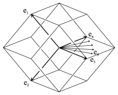
Figure 7: $\Delta$-zonotope $Zono(\Delta_{n})$ as a generalized rhombic dodecahedron.

Example 25.

Figure 7 depicts the standard $(n-1)$-dimensional $\Delta$-zonotope. In the special case $n=4$ one obtains the rhombic dodecahedron.

Definition 26.

The generalized root polytope associated to a simplex $\Delta_{A}={\rm Conv}(A)={\rm Conv}\{a_{1},\dots,a_{n}\}$ is the polytope,

$$Root(\Delta_{A})={\rm Conv}\{a_{i}-a_{j}\mid 1\leqslant i\neq j\leqslant n\}.$$ (28)

If $W$ is an affine map such that $a_{i}=W(e_{i})$ for each $i\in[n]$ then,

$$Root(W(\Delta_{n}))=W(Root(\Delta_{n}))=W(Root_{n}).$$ (29)

The root polytope $Root_{n}$ is a subset of the hyperplane $H_{0}=\{x\in\mathbb{R}^{n}\mid x_{1}+\dots+x_{n}=0\}$ while $Zono(\Delta_{n})\subset H_{n}=\{x\in\mathbb{R}^{n}\mid x_{1}+\dots+x_{n}=n\}$. In the following proposition we claim that the $\Delta$-zonotope $Zono(\Delta_{n}^{0})$, obtained by translating $Zono(\Delta_{n})$ to $H_{0}$, is precisely the polar dual of the polytope $Root_{n}$.

Proposition 27.

The root polytope $Root_{n}={\rm Conv}\{e_{i}-e_{j}\mid 1\leqslant i\neq j\leqslant n\}\subset H_{0}$ is the dual (inside $H_{0}$) of the $\Delta$-zonotope $Zono(\Delta_{n}^{0})$ where $\Delta_{n}^{0}=\Delta_{n}-\frac{1}{n}(e_{1}+\dots+e_{n})$,

$$(Root_{n})^{\circ}=Zono(\Delta_{n}^{0}).$$ (30)

Proof: The proof is an elementary exercise in the concept of duality (see [Ž15, Proposition 7]). Let $\hat{e}_{i}=e_{i}-\frac{1}{n}(e_{1}+\dots+e_{n})\in H_{0}$. It is sufficient to observe that the dual of the root polytope is,

$$(Root_{n})^{\circ}=\{x\in H_{0}\mid|x_{i}-x_{j}|\leqslant 1,\,\mbox{ {\rm for} }1\leqslant i\leqslant n)\},$$ (31)

while the two supporting hyperplanes of $Zono(\Delta_{n}^{0})$, parallel to $\mathcal{L}_{i,j}={\rm span}\{\hat{e}_{k}\mid i\neq k\neq j\}$ (Figure 7) have equations,

$$x_{i}-x_{j}=1\quad\mbox{\rm{and} }\quad x_{j}-x_{i}=1.$$

$\square$

Lemma 28.

Suppose that $K^{\circ}$ is the polar dual of a convex body $K$. If $A:\mathbb{R}^{d}\rightarrow\mathbb{R}^{d}$ is a non-singular linear map then,

$$(A(K))^{\circ}=B(K^{\circ})$$ (32)

where $B=(A^{\ast})^{-1}$. In particular if $A=(A^{\ast})^{-1}$ is an orthogonal transformation and $\mu\neq 0$ then, $(A(K))^{\circ}=A(K^{\circ})$ and $(\mu K)^{\circ}=(1/\mu)K^{\circ}$.

Proof: If $y\in(A(K))^{\circ}$ then by definition,

$$\langle y,Ax\rangle=\langle A^{\ast}y,x\rangle\leqslant 1\quad\mbox{\rm{for each}}\,x\in K.$$ (33)

The following extension of Proposition 27 is recorded for the future reference.

Proposition 29.

Let $H_{0}\subset\mathbb{R}^{n}$ be the subspace spanned by $\hat{e}_{i}=e_{i}-\frac{1}{n}(e_{1}+\dots+e_{n})$ and let $\Delta_{n}^{0}={\rm Conv}\{\hat{e}_{1},\dots,\hat{e}_{n}\}$. Let $A:H_{0}\rightarrow H_{0}$ be a non-singular linear map and let $B:=(A^{\ast})^{-1}$. Then,

$$(Root(A(\Delta_{n}^{0})))^{\circ}=Zono(B(\Delta_{n}^{0}))$$ (34)

Proof: By definition $Root(A(\Delta_{n}^{0}))=A(Root(\Delta_{n}^{0}))$ and $Zono(B(\Delta_{n}^{0}))=B(Zono(\Delta_{n}^{0}))$. It follows from Proposition 27 and Lemma 28 that,

$$(Root(A(\Delta_{n}^{0})))^{\circ}=(A(Root(\Delta_{n}^{0})))^{\circ}=B((Root(\Delta_{n}^{0}))^{\circ})=B(Zono(\Delta_{n}^{0}))=Zono(B(\Delta_{n}^{0})).$$

5.3 $W_{n}^{\circ}$ as a Kantorovich-Rubinstein polytope

There is a canonical isomorphism of vector spaces $H_{\nu}=\{x\in\mathbb{R}^{n}\mid x_{1}+\dots+x_{n}=\nu\}$ and the quotient space $\mathbb{R}^{n}/\mathbb{R}e$, where $e=\frac{1}{n}(e_{1}+\dots+e_{n})$, which induces a canonical isomorphism between $H_{0}$ and $H_{\nu}=\{x\in\mathbb{R}^{n}\mid x_{1}+\dots+x_{n}=\nu\}$ for each $\nu\in\mathbb{R}$.

The canonical isomorphism between $H_{1}$ and $H_{0}$ sends $e_{i}$ to $\hat{e}_{i}=e_{i}-\frac{1}{n}(e_{1}+\dots+e_{n})$ and $\Delta_{n}={\rm Conv}\{{e}_{1},\dots,{e}_{n}\}$ to $\Delta_{n}^{0}={\rm Conv}\{\hat{e}_{1},\dots,\hat{e}_{n}\}$.

The canonical isomorphism between $H_{n}$ and $H_{0}$ identifies the polytope $\Delta_{\mathcal{F}}$, introduced in Section 5.1 (equation (26)), with the polytope,

$$\Delta_{\mathcal{F}}=\sum_{i=1}^{n}~{}[\hat{e}_{i},\hat{e}_{i+1}]=\sum_{i=1}^{n}~{}(\hat{e}_{i}+[0,\hat{e}_{i+1}-\hat{e}_{i}])=\sum_{i=1}^{n}~{}[0,\hat{e}_{i+1}-\hat{e}_{i}]=Zono(B(\Delta_{n}^{0}))$$ (35)

where $e_{n+1}:=e_{1}$ and $B:H_{0}\rightarrow H_{0}$ is the linear map defined by $B(\hat{e}_{i})=b_{i}=\hat{e}_{i+1}-\hat{e}_{i}$. In other words the polytope $\Delta_{\mathcal{F}}$ (associated to the irredundant basis (25) of the building set $\mathcal{\widehat{F}}=Con(C_{n})$) is a $\Delta$-zonotope (generalized rhombic dodecahedron) $Zono(B(\Delta_{n}^{0}))$.

The dual of $Zono(B(\Delta_{n}^{0}))$ is by Proposition 29 a root polytope,

$$Root_{n}^{a}:={\rm Conv}\{a_{i}-a_{j}\mid 1\leqslant i\neq j\leqslant n\}=Root(A(\Delta_{n}^{0}))$$ (36)

where the vectors $\{a_{i}\}_{i=1}^{n}\subset H_{0}$ are defined by $a_{i}=A(\hat{e_{i}})$ and $A:H_{0}\rightarrow H_{0}$ is the linear map such that $B=(A^{\ast})^{-1}$ ($A=(B^{\ast})^{-1}$ ).

Summarizing, we record for the future reference the following proposition,

Proposition 30.

There exist vectors $\{a_{i}\}_{i=1}^{n}\subset H_{0}$, such that $a_{1}+\dots+a_{n}=0$ and ${\rm Span}(\{a_{i}\}_{i=1}^{n})=H_{0}$, which have the property that the dual of the root polytope $Root_{n}^{a}$ (defined by (36)) is the polytope $\Delta_{\mathcal{F}}$ (defined by (35)).

The following theorem is the main result of Section 5.

Theorem 31.

There exists a quasi-metric (asymmetric distance function) $\rho$ on the set $[n]$ such that the associated Kantorovich-Rubinstein polytope,

$$KR(\rho)={\rm Conv}\left\{\frac{e_{i}-e_{j}}{\rho(i,j)}\mid 1\leqslant i\neq j\leqslant n\right\}$$ (37)

is affinely isomorphic to the dual $W_{n}^{\circ}$ of the cyclohedron $W_{n}$. Moreover the distance function $\rho$ satisfies a strict triangle inequality in the sense that,

$$\rho(i,k)<\rho(i,j)+\rho(j,k)\,\mbox{ {\rm if} }\,i\neq j\neq k\neq i.$$

Proof: Let $\{a_{i}\}_{i=1}^{n}\subset H_{0}$ be the collection of vectors described in Proposition 30 and let $a_{i,j}=a_{i}-a_{j}$ (for $1\leqslant i\neq j\leqslant n$) be the corresponding roots. In light of Proposition 30 the polytope $\Delta_{\mathcal{F}}$ has the following description,

$$\Delta_{\mathcal{F}}=\{x\in H_{0}\mid\langle a_{i,j},x\rangle\leqslant 1\,\mbox{ {\rm for each pair} }\,i\neq j\}.$$ (38)

All inequalities in (38) are irredundant. Moreover, the analysis from Section 5.1 guarantees that there exist positive real numbers $\{\alpha_{i,j}\mid 1\leqslant i\neq j\leqslant n\}$ such that,

$$W_{n}=\Delta_{\mathcal{\widehat{F}}}=\{x\in H_{0}\mid\langle a_{i,j},x\rangle\leqslant\alpha_{i,j}\,\mbox{ {\rm for each pair} }\,i\neq j\}.$$ (39)

From here it immediately follows that,

$$W_{n}^{\circ}={\rm Conv}\left\{\frac{a_{i,j}}{\alpha_{i,j}}\mid 1\leqslant i\neq j\leqslant n\right\}.$$

Let us show that $\rho(i,j):=\alpha_{i,j}$ is a strict quasi-metric on $[n]$. Assume that there exist three, pairwise distinct, indices $i.j.k\in[n]$ such that $\rho(i,k)\geqslant\rho(i,j)+\rho(j,k)$. Then,

$$\frac{a_{i,k}}{\rho(i,k)}\in[0,a_{i,k}/(\rho(i,j)+\rho(j,k))]\quad\mbox{{\rm and}}\quad\frac{a_{i,k}}{\alpha_{i,k}}\in[0,a_{i,k}/(\alpha_{i,j}+\alpha_{j,k}))].$$

In light of the obvious equality,

$$\frac{a_{i,k}}{\alpha_{i,j}+\alpha_{j,k}}=\frac{\alpha_{i,j}}{\alpha_{i,j}+\alpha_{j,k}}\left(\frac{a_{i,j}}{\alpha_{i,j}}\right)+\frac{\alpha_{j,k}}{\alpha_{i,j}+\alpha_{j,k}}\left(\frac{a_{j,k}}{\alpha_{j,k}}\right)$$

we observe that if both inequalities,

$$\langle a_{i,j},x\rangle\leqslant\alpha_{i,j}\quad\mbox{{\rm and}}\quad\langle a_{j,k},x\rangle\leqslant\alpha_{j,k}$$

are satisfied then $\langle a_{i,k},x\rangle\leqslant\alpha_{i,k}$. This is however in contradiction with non-redundancy of the last inequality in the representation (39). $\square$

5.4 An explicit quasi-metric associated to a cyclohedron

Definition 32.

Let $\mathcal{\widehat{F}}$ be the building closure of a hypergraph $\mathcal{F}\subset 2^{[n]}\setminus\{\emptyset\}$. The associated ‘height function’ $h_{\mathcal{F}}:\mathcal{\widehat{F}}\rightarrow\mathbb{R}$ is defined by,

$$h_{\mathcal{F}}(X)=\frac{|\mathcal{F}|}{n}-\frac{|\mathcal{F}_{X}|}{|X|},$$

so in particular $h_{\mathcal{F}}([n])=0$ for each hypergraph $\mathcal{F}$.

The inequalities (23), describing $\Delta_{F}$ as a subset of $H_{|\mathcal{F}|}=\{x\in\mathbb{R}^{n}\mid\phi_{[n]}(x)=|\mathcal{F}|\}$ can be, with the help of the height function, rewritten as follows,

$$\Delta_{\mathcal{F}}=\left\{x\in H_{|\mathcal{F}|}\mid\mbox{ {\rm For each} }\,X\in\mathcal{\widehat{F}}\setminus\{[n]\},\,\frac{\phi_{[n]}(x)}{n}-\frac{\phi_{X}(x)}{|X|}\leqslant h_{\mathcal{F}}(X)\right\}.$$ (40)

In particular, if $\mathcal{F}=\mathcal{\widehat{F}}$ we obtain the representation,

$$\Delta_{\mathcal{\widehat{F}}}=\left\{x\in H_{|\mathcal{\widehat{F}}|}\mid\mbox{ {\rm For each} }\,X\in\mathcal{\widehat{F}}\setminus\{[n]\},\,\frac{\phi_{[n]}(x)}{n}-\frac{\phi_{X}(x)}{|X|}\leqslant h_{\mathcal{\widehat{F}}}(X)\right\}.$$ (41)

Assuming that $h_{\mathcal{F}}(X)\neq 0$ for each $X\in\mathcal{\widehat{F}}\setminus\{[n]\}$, let $A_{X}\in H_{0}$ be the vector defined by,

$$A_{X}:=\frac{1}{h_{\mathcal{F}}(X)}\left(\frac{e}{n}-\frac{e_{X}}{|X|}\right),$$ (42)

where $e_{X}:=\sum_{i\in X}~{}e_{i}$ and $e=e_{[n]}=e_{1}+\dots+e_{n}$. It follows that (40) and (41) can be rewritten as,

$$\Delta_{\mathcal{F}}=\left\{x\in H_{0}\mid\mbox{ {\rm For each} }\,X\in\mathcal{\widehat{F}}\setminus\{[n]\},\,\langle A_{X},x\rangle\leqslant 1\right\},$$ (43)

$$\Delta_{\widehat{\mathcal{F}}}=\left\{x\in H_{0}\mid\mbox{ {\rm For each} }\,X\in\mathcal{\widehat{F}}\setminus\{[n]\},\,\langle A_{X},x\rangle\leqslant\frac{h_{\mathcal{\widehat{F}}}(X)}{h_{\mathcal{F}}(X)}\right\}.$$ (44)

Now we specialize to the case $\mathcal{F}:=\{\{1,2\},\{2,3\},\dots,\{n-1,n\},\{n,1\}\}$, so the associated building closure $\mathcal{\widehat{F}}=Con(C_{n})$ is, as in Proposition 23, the building set of all $C_{n}$-connected subsets (circular intervals) in the circle graph $C_{n}$ . The corresponding height functions are shown in the following lemma.

Lemma 33.

If $X=[n]$ then $h_{\mathcal{F}}(X)=h_{\mathcal{\widehat{F}}}(X)=0$. If $X\neq[n]$ then,

$$h_{\mathcal{F}}(X)=\frac{1}{|X|}\quad\mbox{ {\rm and} }\quad h_{\mathcal{\widehat{F}}}(X)=\frac{n^{2}-n+1}{n}-\frac{|X|+1}{2}.$$

Recall (Section 3.1) that for $i,j\in{\rm Vert}(C_{n})=[n]$, the associated (discrete) circular interval is $[i,j]^{0}:=[i,j]\cap[n]$. Similarly (for $i\neq j$) $[i,j)^{0}:=[i,j)\cap[n]$, so $[i,j)^{0}=[i,j-1]^{0}$ if $i\neq j$ and $[i,i)^{0}=\emptyset$ . Define the “clock quasi-metric” on ${\rm Vert}(C_{n})$ by,

$$d(i,j):=|[i,j)^{0}|=|[i,j]^{0}|-1.$$ (45)

Proposition 34.

Let $\rho$ be the quasi-metric on $[n]={\rm Vert}(C_{n})$ defined by,

$$\rho(i,j)=d(i,j)\frac{n^{2}-n+1}{n}-\frac{d(i,j)(d(i,j)+1)}{2}$$ (46)

where $d$ is the clock quasi-metric on $[n]$. Than the associated Kantorovich-Rubinstein polytope $KR(\rho)$ is affinely isomorphic to a polytope dual to the standard cyclohedron.

Proof: By definition $\rho(i,j)=h_{\mathcal{\widehat{F}}}([i,j)^{0})/h_{\mathcal{F}}([i,j)^{0})$. Recall that equations (43) and (44) are nothing but a more explicit form of equations (38) and (39). It immediately follows that $\rho(i,j)=\alpha_{i,j}$ which by Theorem 31 implies that $\rho$ is indeed a quasi-metric on $[n]$ such that the associated Lipschitz polytope $Lip(\rho)$ is a cyclohedron. $\square$

Remark 35.

By a similar argument we already know that vectors $\{A_{X}\mid X\in\mathcal{\widehat{F}}\setminus\{[n]\}\}$, described by equation (42), form a type A root system if $\mathcal{F}:=\{\{1,2\},\{2,3\},\dots,\{n,1\}\}$. This can be seen directly as follows. For $2\leq i\leq n$, let $X_{i}:=[1,i)^{0}$ and $A_{i}:=A_{X_{i}}$. Then there is a disjoint union,

$$\{A_{X}\mid X\in\mathcal{\widehat{F}}\setminus\{[n]\}\}=\{A_{i}\}_{i=2}^{n}\sqcup\{-A_{i}\}_{i=2}^{n}\sqcup\{A_{i}-A_{j}\mid 2\leq i\neq j\leq n\}.$$

This observation and a comparison of (35) and (43) provide an alternative proof of Proposition 27.

6 Alternative approaches and proofs

An elegant and versatile analysis of the combinatorial structure of Lipschitz polytopes, conducted by Gordon and Petrov in [GP], can be with little care (but without introducing any new ideas) extended to the case of quasi-metrics.

This fact, as kindly pointed by an anonymous referee, provides a method for describing a large class of quasi-metrics which are combinatorially of “cyclohedral type”.

Here we give an outline of this method. (This whole section can be seen as a short addendum to the paper [GP].)

A combinatorial structure on the (dual) pair of polytopes $Lip(\rho)$ and $KR(\rho)$ is, following [GP, Definition 2], the collection of directed graphs $\mathcal{D}(\rho)=\{D(\alpha)\mid\alpha\mbox{ {\rm is a face of} }KR(\rho)\}$, where for each face $\alpha$ of $KR(\rho)$,

$$(i,j)\in D(\alpha)\quad\Leftrightarrow\quad\frac{e_{j}-e_{i}}{\rho(i,j)}\in\alpha.$$

Following [GP, Definition 1], a quasi-metric is generic if the triangle inequality is strict ($x\neq y\neq z\Rightarrow\rho(x,z)<\rho(x,y)+\rho(y,z)$) and the polytope $KR(\rho)$ is simplicial ($Lip(\rho)$ is simple).

In the case of a generic quasi-metric, the combinatorial structure $\mathcal{D}(\rho)$ is a simplicial complex whose face poset is isomorphic to the face poset of the polytope $KR(\rho)$ (see Corollary 1 and Theorem 4 in [GP]). Moreover, in this case $D(\alpha)$ is a directed forest (such that either the in-degree or the out-degree of each vertex is zero), and in particular if $\alpha$ is a facet then $D(\alpha)$ is a directed tree.

Following [GP, Theorem 3] (see also [GP, Theorem 4]) a directed tree (forest) $T$ is in $\mathcal{D}(\rho)$ if and only if it satisfies a “cyclic monotonicity” condition (inequality (1) in [GP, Theorem 3]), indicating that $T$ can be thought of as an ‘optimal transference plan’ for the transport of the corresponding measures.

It was shown in Section 3 (Proposition 7) that the face poset of a cyclohedron can be also described as a poset of directed trees (corresponding to the diagrams of oriented arcs, as exemplified by Figures 2 and 3).

From these observations arises a general plan for finding a generic quasi-metric $\rho$ such that the associated combinatorial structure $\mathcal{D}(\rho)$ is precisely the collection of trees associated to a cyclohedron. Moreover, this approach allows us (at least in principle) to characterize all generic quasi-metrics of “combinatorial cyclohedral type”.

Indeed, if $\rho=(\rho(i,j))_{1\leq i,j\leq n}$ is an unknown quasi-metric (ranging over the space of all quasi-metric matrices), then one can characterize quasi-metrics of cyclohedral type by writing all inequalities of the type (1) in [GP, Theorem 3] (see also the simplification provided by [GP, Theorem 4]).

Remark 36.

Guided by the form of the metric $\rho$, described by the formula (46) (Proposition 34), the referee observed that the quasi-metric $\rho_{\epsilon}:=d-\epsilon\cdot d^{2}$ (where $d$ is the clock quasi-metric and $\epsilon>0$ a sufficiently small number), is a good candidate for a cyclohedral quasi-metric. (The details of related calculations will appear elsewhere.)

Remark 37.

The quasi-metric $\rho$ introduced in Proposition 34 is somewhat exceptional since in this case we guarantee that $KR(\rho)$ is geometrically (affinely) and not only combinatorially (via face posets) isomorphic to a dual of a standard cyclohedron. This has some interesting consequences, for example this metric has the property that the associated Lipschitz polytope $Lip(\rho)$ is a Delzant polytope.

7 Concluding remarks

7.1 The result of Gordon and Petrov

The motivating result of J. Gordon and F. Petrov [GP, Theorem 1] says that for a generic metric $\rho$ on a set of size $n+1$, the number of $(n-i)$-dimensional faces of the associated Lipschitz polytope (the dual of $KR(\rho)$, see the equation (1)) is equal to,

$$f_{n-i}(Lip(\rho))={{n+i}\choose{i,i,n-i}}=\frac{(n+i)!}{i!i!(n-i)!}.$$

The link with the combinatorics of cyclohedra, established by Theorems 14 and 31, allows us to deduce this result from the known calculations of $f$-vectors of these polytopes. For example R. Simion in [Si, Proposition 1] proved that,

$$f_{i-1}(W_{n})={n\choose i}{n+i\choose i}=\frac{(n+i)!}{i!i!(n-i)!}.$$

Moreover, in light of Theorems 14 and 31, the generating series for these numbers have a new interpretation as a solution of a concrete partial differential equation, see for example [BP, Sections 1.7. and 1.8.].

7.2 Tight hypergraphs

The relationship between the cyclohedron and the (dual of the) root polytope is explained in Section 5 as a special case of the relationship between tight hypergraphs $\mathcal{F}$ and their building closures $\mathcal{\widehat{F}}$. For this reason it may be interesting to search for other examples of ‘tight pairs’ $(\mathcal{\widehat{F}},\mathcal{F})$ of hypergraphs.

Example 38.

Let $C_{n}$ be the cycle graph on $n$ vertices (identified with their labels [n]) and let $\prec$ be the associated (counterclockwise) cyclic order on $[n]$. For each ordered pair $(i,j)$ of indices let $[i,j]^{0}:=\{i,i+1,\dots,j\}$ be the associated ‘cyclic interval’. For each $2\leq k\leq n-1$ let $BC_{n}^{k}\subset 2^{[n]}\setminus\{\emptyset\}$ be the hypergraph defined by,

$$BC_{n}^{k}:=\{[1,k]^{0},[2,k+1]^{0},\dots,[n,k-1]^{0}\}.$$ (47)

Then $BC_{n}^{k}$ is a tight hypergraph on $[n]$. Moreover, if $\widehat{\mathcal{F}}_{n,k}:=\widehat{BC}_{n}^{k}$ is its building closure and $Q_{n,k}:=\Delta_{\widehat{\mathcal{F}}_{n,k}}$ the associated simple polytope than for $k\neq k^{\prime}$ the associated polytopes $Q_{n,k}$ and $Q_{n,k^{\prime}}$ are combinatorially non-isomorphic.

Note that for $k=2$ we recover the tight hypergraph described in Proposition 23 (equation (25)) and in this case $Q_{n,2}=W_{n}$. Moreover observe that,

$$\mathcal{N}_{n,2}\varsupsetneq\mathcal{N}_{n,3}\supsetneq\dots\supsetneq\mathcal{N}_{n,n-1},$$

where $\mathcal{N}_{n,k}$ is the poset of nested sets in $\widehat{\mathcal{F}}_{n,k}$, which immediately implies that $Q_{n,k}\ncong Q_{n,k^{\prime}}$ for $k\neq k^{\prime}$.

7.3 Canonical quasitoric manifold over a cyclohedron

The cyclohedron $W_{n}$, together with the associated canonical map $\phi_{n}$, restricted to the set of vertices of $W_{n}^{\circ}$ ($\leftrightarrow$ the set of facets of $W_{n}$), defines a combinatorial quasitoric pair $(W_{n},\phi_{n})$ in the sense of [BP, Definition 7.3.10]. Indeed, if $F_{1},\dots,F_{n-1}$ are distinct facets of $W_{n}$ such that $\cap_{i=1}^{n-1}~{}F_{i}\neq\emptyset$, then the corresponding dual vertices $v_{1},\dots,v_{n-1}$ of $W_{n}^{\circ}$ span a simplex and the vectors $\phi(v_{1}),\dots,\phi(v_{n-1})$ form a basis of the associated type A root lattice $\Lambda_{n}\cong\mathbb{Z}^{n-1}$ (spanned by the vertices of the root polytope $Root_{n}$).

We refer to the associated quasitoric manifold $M=M_{(W_{n},\phi_{n})}$ as the canonical quasitoric manifold over a cyclohedron $W_{n}$.

7.4 The cyclohedron and the self-linking knot invariants

It may be expected that the combinatorics of the map $\phi:W_{n}^{\circ}\rightarrow Root_{n}$, as illustrated by Theorems 14 and 31 (and their proofs), may be of some relevance for other applications where the cyclohedron $W_{n}$ played an important role. Perhaps the most interesting is the role of the cyclohedron in the combinatorics of the self-linking knot invariants (Bott and Taubes [BT], Volić [Vo]). Other potentially interesting applications include some problems of discrete geometry, as exemplified by the ‘polygonal pegs problem’ [VZ] and its relatives.

Acknowledgements: The project was initiated during the program ‘Topology in Motion’, https://icerm.brown.edu/programs/sp-f16/, at the Institute for Computational and Experimental Research in Mathematics (ICERM, Brown University). With great pleasure we acknowledge the support, hospitality and excellent working conditions at ICERM. The research of Filip Jevtić is a part of his PhD project at the University of Texas at Dallas, performed under the supervision and with the support of Vladimir Dragović. We would also like to thank the referee for very useful comments and suggestions, in particular for the observations incorporated in Section 6.

References

- [A+] F. Ardila, M. Beck, S. Ho̧sten, J. Pfeifle, and K. Seashore, Root polytopes and growth series of root lattices, SIAM J. Discrete Math. 25 (2011), no. 1, 360–378.
- [Ba] M.M. Bayer. Equidecomposable and weakly neighborly polytopes, Israel J. Math. 81 (1993), 301–320.
- [BT] R. Bott, C. Taubes, On the self-linking of knots, J. Math. Phys. 35:10 (1994), 5247–5287.
- [BP] V. Buchstaber, T. Panov. Toric Topology, Mathematical Surveys and Monographs, 204, Amer. Math. Soc., Providence, RI, 2015.
- [DH] E. Delucchi, L. Hoessly. Fundamental polytopes of metric trees via hyperplane arrangements, arXiv:1612.05534 [math.CO].
- [CD] M. Carr, S.L. Devadoss. Coxeter complexes and graph-associahedra, Topology and its Applications 153 (2006), 2155–2168.
- [De] S.L. Devadoss. A space of cyclohedra, Discrete and Computational Geometry 29 (2003), 61–75.
- [DP] K. Došen, Z. Petrić. Hypergraph polytopes, Topology Appl., 158 (2011), 1405–1444.
- [FS] E.M. Feichtner, B. Sturmfels. Matroid polytopes, nested sets and Bergman fans. Port. Math. (N.S.) 62 (2005), 4, 437–468.
- [GGP] I. M. Gelfand, M. I. Graev, A. Postnikov. Combinatorics of hypergeometric functions associated with positive roots, in Arnold-Gelfand Mathematical Seminars: Geometry and Singularity Theory, Birkhäuser, Boston, 1996, 205–221.
- [GKZ] I. M. Gelfand, M. M. Kapranov, A. V. Zelevinsky. Discriminants, resultants, and multidimensional determinants, Birkhäuser, 1994.
- [GP] J. Gordon, F. Petrov. Combinatorics of the Lipschitz polytope. Arnold Math. J. 3 (2), 205–218 (2017). arXiv:1608.06848 [math.CO].
- [] J. De Loera, J. Rambau, F. Santos. Triangulations: Structures for Algorithms and Applications, Springer 2010.
- [M99] M. Markl, Simplex, associahedron, and cyclohedron, in Higher Homotopy Structures in Topology and Mathematical Physics (J. McCleary, ed.), Contemporary Math., 227, Amer. Math. Soc., 1999, 235–265.
- [MPV] J. Melleray, F. Petrov, A. Vershik. Linearly rigid metric spaces and the embedding problem. Fundam. Math., 199(2):177–194, 2014.
- [Po] A. Postnikov. Permutohedra, associahedra, and beyond. Int. Math. Res. Not. 2009, 6, 1026–1106.
- [PRW] A. Postnikov, V. Reiner, L. Williams. Faces of generalized permutohedra. Doc. Math. 13 (2008), 207–273.
- [Si] R. Simion. A type-B associahedron, Adv. in Appl. Math. 30 (2003), 2–25.
- [Sta] J. Stasheff. From operads to ‘physically’ inspired theories, in Operads: Proceedings of Renaissance Conferences (J-L. Loday, J.D. Stasheff, A. Voronov, eds.), Contemporary Math., 202, Amer. Math. Soc., 1997, 53–81.
- [Ve1] A.M. Vershik. Long history of the Monge-Kantorovich transportation problem. Math. Intell., 32(4):1–9, 2013.
- [Ve2] A.M. Vershik. The problem of describing central measures on the path spaces of graded graphs. Funct. Anal. Appl., 48(4):26–46, 2014.
- [Ve3] A.M. Vershik. Classification of finite metric spaces and combinatorics of convex polytopes. Arnold Math. J., 1(1):75–81, 2015.
- [Vi1] C. Villani. Topics in Optimal Transportation, Graduate Studies in Mathematics Vol. 58, Amer. Math. Soc. 2003.
- [Vi2] C. Villani. Optimal Transport: Old and New, Springer Verlag (Grundlehren der mathematischen Wissenschaften), 2009.
- [Vo] I. Volić. Configuration space integrals and the topology of knot and link spaces, Morfismos 17 (2013), no. 2, 1–56.
- [VZ] S. Vrećica, R. T. Živaljević, Fulton-MacPherson compactification, cyclohedra, and the polygonal pegs problem, Israel J. Math. 184 (2011), no. 1, 221–249.
- [Ž15] R.T. Živaljević. Illumination complexes, -zonotopes, and the polyhedral curtain theorem, Comput. Geom., 48 (2015) 225–236.