Lensing of Fast Radio Bursts by Plasma Structures in Host Galaxies

Abstract

Plasma lenses in the host galaxies of fast radio bursts (FRBs) can strongly modulate FRB amplitudes for a wide range of distances, including the $\sim$ Gpc distance of the repeater FRB121102. To produce caustics, the lens’ dispersion-measure depth (${\rm DM}_{\ell}$), scale size ($a$), and distance from the source ($d_{\rm sl}$) must satisfy ${\rm DM}_{\ell}d_{\rm sl}/a^{2}\gtrsim 0.65~{}{\rm pc^{2}\ AU^{-2}\ cm^{-3}}$. Caustics produce strong magnifications ($\lesssim 10^{2}$) on short time scales ($\sim$ hours to days and perhaps shorter) along with narrow, epoch dependent spectral peaks (0.1 to 1 GHz). However, strong suppression also occurs in long-duration ($\sim$ months) troughs. When bursts are multiply imaged, they will arrive differentially by $<1~{}\mu$s to tens of ms and they will show different apparent dispersion measures, $\delta{\rm DM}_{\rm apparent}\sim 1$ pc cm^-3. Arrival time perturbations may mask any underlying periodicity with period $\lesssim 1$ s. When arrival times differ by less than the burst width, interference effects in dynamic spectra will be seen. Strong lensing requires source sizes smaller than $({\rm Fresnel~{}scale)^{2}}/a$, which can be satisfied by compact objects such as neutron star magnetospheres but not by AGNs. Much of the phenomenology of the repeating fast radio burst source FRB121102 can be accounted for with such lenses. The overall picture can be tested by obtaining wideband spectra of bursts (from $<1$ to 10 GHz and possibly higher), which can also be used to characterize the plasma environment near FRB sources. A rich variety of phenomena is expected from an ensemble of lenses near the FRB source. We discuss constraints on densities, magnetic fields, and locations of plasma lenses related to requirements for lensing to occur.

1 Introduction

Fast radio bursts (FRBs) are millisecond duration pulses that show dispersive arrival times like those seen from Galactic pulsars and that are consistent with the cold plasma dispersion law (e.g. Thornton et al., 2013). The dispersion measures (DM, the column density of free electrons along the line of sight) of FRBs are too large to be accounted for by Galactic models of the ionized interstellar medium (ISM) in the Milky Way (e.g. Cordes & Lazio, 2002; Yao et al., 2016). However it is only with the measurement of the redshift of the host galaxy firmly associated with the repeating FRB121102 (Chatterjee et al., 2017; Marcote et al., 2017; Tendulkar et al., 2017) that the extragalactic nature of an FRB has been confirmed without qualification. It is likely that most if not all of the other $\sim 20$ reported FRBs are also extragalactic, though it is unclear whether FRB121102 is representative of all FRBs in other respects.

The multiple bursts obtained from FRB121102 display striking spectral diversity within the passbands of hundreds of MHz used at $\nu\sim 1.5$ GHz. Single burst spectra show rises toward lower frequencies in some cases and rises toward higher frequencies or midband maxima in other; burst shapes also show evolution with frequency across the band (Spitler et al., 2014, 2016; Scholz et al., 2016). Very surprising are the changes in spectral signatures that occur on time scales less than one minute. The repetition rate of the source is episodic and intermittent, with quiet periods of weeks to months separating observation epochs where bursts occur. A detailed study of burst occurrence rates and morphologies in time and frequency is forthcoming (J. Hessels, in preparation).

These phenomena suggest that extrinsic propagation phenomena may play a role along with spectro-temporal variability intrinsic to the source. Gravitational lensing or microlensing by themselves cannot be responsible for burst magnification because burst amplitudes of FRB121102 are highly chromatic. Standard interstellar scintillation (Rickett, 1990) from the Milky Way can also be ruled out because diffractive scintillations (DISS) are highly quenched by bandwidth averaging for the line of sight through the Galactic plane to FRB121102. Many ‘scintles’ with characteristic bandwidths $\sim 60$ kHz at 1.4 GHz (estimated with the NE2001 model; Cordes & Lazio, 2002) are averaged over the 300 to 600 MHz bandwidths used at Arecibo, yielding a DISS modulation fraction of only a few per cent. Refractive scintillations typically only cause modulations of tens of per cent and vary on time scales significantly longer than DISS; also, they do not introduce any narrow spectral structure. Strong focusing by plasma lenses is the most likely process because it can produce large variations (factors of ten to 100) that could account for much of the intermittency seen from FRB 121102.

Plasma lensing from $\sim$ AU structures in the Milky Way are consistent with ‘extreme scattering’ events (ESEs) seen in the light curves of a few active galactic nuclei (AGNs; Fiedler et al., 1987; Bannister et al., 2016) and pulsars along with timing perturbations for the latter objects (Coles et al., 2015). Required densities indicate they are over-pressured with respect to the mean ISM but by an amount that is minimized if events occur when plasma filaments or sheets are edge on to the line of sight. Very strong overpressure in about 0.05% of neutral gas in the cold ISM (Jenkins & Tripp, 2011) is attributed to turbulence driven by stellar winds or supernovae. There is no consensus on the relationship of ESE lenses to other interstellar structures (e.g. Romani et al., 1987; Walker & Wardle, 1998; Pen & Levin, 2014). However, a common feature may be edge-on alignment of structures inferred for both Galactic plasma lenses and cold HI (Romani et al., 1987; Heiles, 1997). It is therefore especially notable that plasma lensing is manifested in distinctive DM variations of the Crab pulsar from dense filaments in the Crab Nebula. Graham Smith et al. (2011) infer diameters $\sim 2$ AU and DM depths $\sim 0.1$ pc cm^-3 from DM variations whereas observations of optical filaments indiciate larger sizes $\sim 1000\,{\rm AU}\times 0.5$ pc with electron densities $n_{\rm e}\sim 10^{4}$ cm^-3 (Davidson & Fesen, 1985).

In this paper we consider lensing from one-dimensional plasma structures in the host galaxy of FRB121102, like the Gaussian lens analyzed by Clegg et al. (1998). One-dimensional lenses show complex properties that may be sufficient to account for the observations of the repeating FRB. Moreover, one-dimensional structures may be physically relevant given that long filaments are seen in the Crab Nebula and it is possible that FRB121102 is associated with a young neutron star in a supernova remnant (e.g. Pen & Connor, 2015; Cordes & Wasserman, 2016; Connor et al., 2016; Metzger et al., 2017; Chatterjee et al., 2017; Marcote et al., 2017; Tendulkar et al., 2017).

In § 2 we derive the general properties of plasma lenses with emphasis on those that are much closer to the source than to us. In § 3 we discuss their application to FRBs while § 4 discusses filaments in the Crab Nebula and their lensing properties. § 5 presents detailed results for an example lens that can account for many of the properties of FRB121102. We discuss our results and make conclusions in § 6. Appendix A elaborates on our use of the Kirchhoff diffraction integral (KDI) of the Gaussian lens.

2 Optics of a Single Plasma Lens

Clegg et al. (1998) analyzed the properties of a one-dimensional (1D) Gaussian plasma lens as a means for understanding discrete events in the light curves of AGNs. Their analysis assumed incidence of plane waves on Galactic lenses of the form ${\rm DM}(x)={\rm DM}_{\ell}\exp{(-x^{2}/a^{2})}$, that yield a phase perturbation $\phi_{\lambda}=-\lambda r_{\rm e}{\rm DM}(x)$, where $\lambda$ is the radio wavelength and $r_{\rm e}$ is the classical electron radius. The lens has a characteristic scale $a$ and the maximum electron column density through the lens is ${\rm DM}_{\ell}$. While a positive column density ${\rm DM}_{\ell}>0$ acts as a diverging lens, rays that pass through different parts of the lens can converge to produce caustics. Two dimensional lenses and the inversion of measurements of lensing events into DM profiles have been considered by Tuntsov et al. (2016).

We extend the analysis of Clegg et al. (1998) to the more general case where a source is at a finite distance from the lens. Let $d_{\rm sl}$ and $d_{\rm so}$ be the distances from the source to the lens and observer, respectively, which define the lens-observer distance $d_{\rm lo}=d_{\rm so}-d_{\rm sl}$.

Transverse coordinates in the source, lens, and observer’s planes are $x_{\rm s},x,$ and $x_{\rm obs}$, respectively, and we define dimensionless coordinates $u_{\rm s}=x_{\rm s}/a$, $u=x/a$, and $u_{\rm obs}=x_{\rm obs}/a$ by scaling them by the lens scale $a$. The lens is centered on $u=0$. We also define a combined offset

$$u^{\prime}=(d_{\rm lo}/d_{\rm so})u_{\rm s}+(d_{\rm sl}/d_{\rm so})u_{\rm obs}.$$ (1)

Offsets or motions of the source dominate $u^{\prime}$ for lenses close to the source ($d_{\rm sl}/d_{\rm so}\ll 1$), while the observer’s location dominates $u^{\prime}$ for Galactic lenses with $1-d_{\rm sl}/d_{\rm so}\ll 1$.

The lens equation in geometric optics corresponds to stationary phase solutions for $u$ of the Kirchhoff diffraction integral (Appendix A),

$$u(1+\alpha e^{-u^{2}})=u^{\prime},$$ (2)

where $\alpha$ is the dimensionless parameter

$$\alpha = \frac{\lambda^{2}r_{\rm e}{\rm DM}_{\ell}}{\pi a^{2}}\left(\frac{d_{\rm sl}d_{\rm lo}}{d_{\rm so}}\right)=\frac{3430\,{\rm DM}_{\ell}d_{\rm sl}}{(\nu a_{\rm AU})^{2}}\left(\frac{d_{\rm lo}}{d_{\rm so}}\right),$$ (3)

where $\nu$ is in GHz, ${\rm DM}_{\ell}$ has standard units of pc cm^-3, the lens scale $a$ is in AU, and the source-lens distance $d_{\rm sl}$ is in kpc. Ray tracings depend only on $\alpha$ and therefore are the same for a wide variety of lens sizes, DMs, and locations.

Electron density enhancements give positive values of $\alpha$ while voids in an otherwise uniform density correspond to $\alpha<0$ and yield a converging rather than a diverging lens. We restrict our analysis to density enhancements in this paper because they are sufficiently rich in phenomena to perhaps account for FRB properties. However, we note that density voids also may be relevant to plasmas surrounding FRB sources. Most of the equations presented here are valid for ${\rm DM}_{\ell}<0$, but require an absolute value in some cases. Lensing is qualitatively similar to the ${\rm DM}_{\ell}>0$ case but the locations of caustics differ.

While we use the 1D Gaussian lens in most of this paper, the basic approach can be applied to an arbitrary 2D perturbation, ${\rm DM}({\mathbf{x}})={\rm DM}_{\ell}\psi({\mathbf{x}})$ where $\psi({\mathbf{x}})$ is a dimensionless function with unity maximum. In this case the lens equation is ${\bf u}^{\prime}={\bf u}+\alpha a\nabla_{\bf u}\psi({\bf u})$ and $a$ is a characteristic scale of $\psi({\bf u})$.

For a given offset $u^{\prime}$ there are either one or three solutions for $u$, as shown in Figure 1 for three values of $u^{\prime}$. For this figure $\alpha=1524\nu^{-2}$, which is given by ${\rm DM}_{\ell}=1$ pc cm^-3, $a=1$ AU, $d_{\rm so}=1$ Gpc and $d_{\rm sl}=1$ kpc but could also correspond to substantially different lens parameters, such as a much smaller $d_{\rm sl}$ combined with larger ${\rm DM}_{\ell}/a^{2}$. In this case $u^{\prime}$ is totally dominated by motions of the source because $d_{\rm sl}/d_{\rm so}=10^{-6}$. However, the same ray traces apply to the Galactic case when the lens is 1 kpc from the Earth. In that case, motions of the observer and lens will dominate changes in the line of sight.

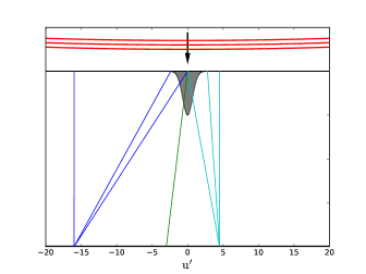
Figure 1: Ray traces from the lens plane to three locations in the transverse plane. Three rays reach the two transverse positions at $u^{\prime}\sim-16$ and $+4.5$ while only one reaches $u^{\prime}\sim-3.5$. The ray tracing is for $\alpha=1524$ which corresponds to ${\rm DM}_{\ell}=1$ pc cm^-3  $a=1$ AU, $d_{\rm sl}=1$ kpc, $d_{\rm so}=1$ Gpc, and $\nu=1.5$ GHz but could correspond to other combinations of parameters. For lenses near a fixed source at $u_{\rm s}=0$, the change in observer’s position $u_{\rm obs}$ needed to yield a unit change in $u^{\prime}$ is $d_{\rm so}/d_{\rm sl}\gg 1$.

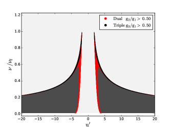
Figure 2: Regions in the frequency – location plane where either one or three images are seen. The frequency $\nu$ has been normalized by the focal frequency $\nu_{\rm f}$ (Eq. 8) and the location $u^{\prime}$ is a linear combination of the source’s and observer’s positions given by Eq. 1. Off white indicates the region where single-images occur while three images occur elsewhere. Red and black show where two or three images occur with approximately equal gain ratios. The red region is where the second largest gain is at least 50% of the largest gain while black indicates where all three images have gains within 50% of each other.

Figure 2 shows the regions in the $\nu$-$u^{\prime}$ plane where either one or three subimages are seen. The frequency axis is expressed in units of a focal frequency $\nu_{\rm f}$ defined below. In dimensional units triple images are seen up to nearly 40 GHz for the case shown. For smaller values of $\alpha$, region of triple images moves to lower frequencies. A single burst from an FRB source can therefore be manifested as three sub-bursts with different amplitudes, DMs, and arrival times for some observer locations and frequencies.

2.1 Amplification

In the geometrical optics regime, the focusing or defocusing of incident wavefronts yields a ‘gain’ (or amplification) given by the stationary-phase solution for $u$ (Appendix A; Clegg et al., 1998),

$$G=\left|1+\alpha(1-2u^{2})e^{-u^{2}}\right|^{-1}.$$ (4)

The variation of $G$ with frequency and transverse location in Figure 3 shows that the highest values occur where there are three images and the lowest values are in a central trough that is aligned with the direction to the lens. Horizontal slices through this plane are shown in Figure 4 at a few frequencies. For triplet images, the total gain is the sum of the gains for the three screen positions $u$ that contribute.

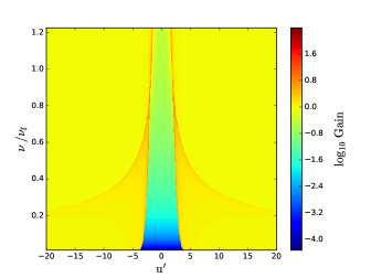
Figure 3: Total gain summed over all rays that reach an observer vs. frequency (normalized by the focal frequency $\nu_{\rm f}$) and transverse location.

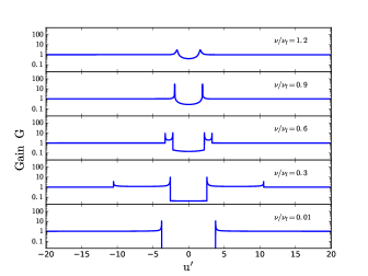
Figure 4: Spatial slices of the gain $G$ for a few frequencies (normalized by the focal frequency $\nu_{\rm f}$).

The minimum gain in the trough is $G_{\rm min}=1/(1+\alpha)$ at $u=u^{\prime}=0$. Some locations are also focal points where $G\to\infty$. These occur for values of $\alpha$,

$$\alpha_{\infty}=\frac{e^{u^{2}}}{2u^{2}-1},$$ (5)

where $u=u(\alpha,u^{\prime})$ is the stationary phase solution of Eq. 2. No infinities occur for $|u|<1/\sqrt{2}$ because $G<1$ when $\alpha$ is restricted to positive values.

The required $\alpha_{\infty}$ diverges at $|u|=1/\sqrt{2}$ and decreases to a minimum $\alpha_{\rm min}=e^{3/2}/2=2.24$ at $|u|=\sqrt{3/2}=1.22$. Diverging gains at larger $|u|>1.22$ require exponentially increasing values of $\alpha_{\infty}$ corresponding to very large densities and distances or to very small lenses that may also produce free-free absorption or may be physically implausible.

To identify locations of infinities numerically, we eliminate $\alpha e^{-u^{2}}$ by combining Eq. 2 and 4 to obtain the algebraic equation, $2u^{3}-2u^{2}u^{\prime}+u^{\prime}=0$. Solutions for $u$ yield the values of $\alpha_{\infty}$ from Eq. 5 needed for the apparent infinity. Actual physical optics gains are finite and can be calculated either through exact evaluation of the Kirchhoff diffraction integral or by integrating the third-order polynomial expansion of the total phase (Appendix A). At $\alpha=\alpha_{\rm min}$ and $u=\sqrt{3/2}$ the maximum gain is

$$G_{\rm max}\sim a/r_{\rm F},$$ (6)

where $r_{\rm F}=\sqrt{\lambda d_{\rm sl}d_{\rm lo}/2\pi d_{\rm so}}$ is the Fresnel scale. Larger lenses therefore give larger maximum gains. We note in Appendix A that the true gain at this location is affected by catastrophe optics (Berry & Upstill, 1980), which describes specific fundamental forms for the large variation of the gain with small changes in position or frequency.

The actual expected gain also depends on the physical size of the source and on any scattering from small-scale irregularities prior to encountering the lens or in the lens itself. A full discussion of these issues is beyond the scope of the paper, although a constraint on source size is given in § 2.7.

2.2 Focal Distance and Focal Frequency

Bursts originating from lens-observer distances $d_{\rm lo}$ larger than a focal distance $d_{\rm f}$ reach the observer on multiple paths and are affected by caustics in light curves. The requirement for multiple images, $\alpha>\alpha_{\rm min}$, gives

$$d_{\rm f}(\nu) = d_{\rm lo}\left(\frac{\alpha_{\rm min}}{\alpha}\right)=\frac{\pi(a\nu)^{2}\alpha_{\rm min}}{r_{\rm e}c^{2}{\rm DM}_{\ell}}\left(\frac{d_{\rm so}}{d_{\rm sl}}\right)$$ (7)

$$\approx 0.65\,{\rm Mpc}\times\frac{(a_{\rm AU}\nu)^{2}}{{\rm DM}_{\ell}}\left(\frac{d_{\rm so}/d_{\rm sl}}{10^{6}}\right),$$

where the coefficient applies to the case where the lens is nearer the source than the observer by a factor of $10^{6}$. Galactic cases with $d_{\rm so}/d_{\rm sl}\sim 1$ can have sub-pc focal distances, which corresponds to a regime where the gain will be close to unity.

A similar analysis implies that frequencies below the focal frequency $\nu_{\rm f}$ will show ray crossings,

$$\nu_{\rm f} = \nu\left(\frac{\alpha}{\alpha_{\rm min}}\right)^{1/2}=\frac{c}{a}\left(\frac{r_{\rm e}{\rm DM}_{\ell}}{\pi\alpha_{\rm min}}\frac{d_{\rm sl}d_{\rm lo}}{d_{\rm so}}\right)^{1/2}$$ (8)

$$\approx 39.1~{}{\rm GHz}\times\frac{{\rm DM}_{\ell}^{1/2}}{a_{\rm AU}}\left(\frac{d_{\rm sl}d_{\rm lo}/d_{\rm so}}{1~{}\rm kpc}\right)^{1/2}.$$

In terms of the focal distance, the focal frequency is $\nu_{\rm f}=\nu\sqrt{d_{\rm lo}/d_{\rm f}(\nu)}$.

2.3 Constraints on Lens Parameters

In their study of AGN light curves, Clegg et al. (1998) considered Galactic lenses with $d_{\rm sl}/d_{\rm so}\sim 1/2$ and $d_{\rm lo}d_{\rm sl}/d_{\rm so}\sim 1~{}$kpc. These give focal values ($d_{\rm f}$ and $\nu_{\rm f}$) similar to the path length through the Galaxy and to the observation frequencies (2.25 and 8.1 GHz) they considered, implying that the ‘extreme scattering events’ they analyzed (Fiedler et al., 1987) were well within the caustic regime.

Lenses embedded in host galaxies of burst sources with $d_{\rm so}/d_{\rm sl}\gg 1$ yield much larger focal distances but similar focal frequencies.

If the observer’s distance is a multiple $M$ of the focal distance (corresponding to $\alpha=M\alpha_{\rm min}$), the lens parameters satisfy

$$\frac{a^{2}}{{\rm DM}_{\ell}}\!=\!\frac{r_{\rm e}c^{2}}{\pi M\alpha_{\rm min}\nu^{2}}\left(\frac{d_{\rm sl}d_{\rm lo}}{d_{\rm so}}\right)\!\approx\!\frac{1531}{M\nu^{2}}\left(\frac{d_{\rm sl}d_{\rm lo}/d_{\rm so}}{1~{}\rm kpc}\right)\!,$$ (9)

where the approximate equality is for $a$ in AU units, $\nu$ in GHz and ${\rm DM}_{\ell}$ in pc cm^-3. Eq. 9 implies that identical lens parameters can satisfy the condition $d_{\rm lo}=Md_{\rm f}$ for either Galactic or extragalactic lenses.

Focal distances equal to the lens distance ($M=1$) may yield a high degree of variability if, for example, a population of lenses moves across the line of sight. Heterogeneous lenses and geometries with different focal distances will produce variability with a range of amplitudes and time scales.

2.4 Times of Arrival (TOA)

Burst arrival times are chromatic due to plasma dispersion along the line of sight. Here we analyze only the TOA perturbations from the plasma lens, which add to delays from other media along the line of sight. For each image produced by the lens, the burst arrival time receives a contribution $t_{\rm g}$ from the geometrical path length of the refracted ray path and from the dispersion delay through the lens. The geometric term is

$$\!\!\!\!\!\!\!t_{\rm g}(x) = (2c)^{-1}\times$$ (10)

$$\!\!\!\!\!\!\!\left[\frac{(x-x_{\rm s})^{2}}{d_{\rm sl}}+\frac{(x-x_{\rm obs})^{2}}{d_{\rm lo}}-\frac{(x_{\rm obs}-x_{\rm s})^{2}}{d_{\rm so}}\right],$$

which vanishes for an unrefracted ray path with $x=(d_{\rm lo}x_{\rm s}+d_{\rm sl}x_{\rm obs})/d_{\rm so}$. The dispersion delay $t_{\rm DM}$ through the lens,

$$t_{\rm DM}(x) = (cr_{\rm e}/2\pi\nu^{2}){\rm DM}(x).$$ (11)

Using dimensionless coordinates and combining the two perturbations, the TOA is

$$t(u)=t_{\rm g_{0}}(u-u^{\prime})^{2}+t_{\rm DM_{0}}e^{-u^{2}},$$ (12)

where the geometrical delay coefficient is

$$t_{\rm g_{0}} = \frac{a^{2}}{2c}\left(\frac{d_{\rm so}}{d_{\rm sl}d_{\rm lo}}\right)$$ (13)

and the dispersion coefficient is

$$t_{\rm DM_{0}} = \alpha t_{\rm DM_{0}}=\frac{cr_{\rm e}{\rm DM}_{\ell}}{2\pi\nu^{2}}=4.149~{}{\rm ms}\times\frac{{\rm DM}_{\ell}}{\nu^{2}},$$ (14)

which is evaluated for frequencies in GHz and DM in standard units of pc cm^-3.

For a specific solution to the lens equation, $u=u(u^{\prime},\alpha)$, the TOA has the simple form

$$t(u) = t_{\rm DM_{0}}e^{-u^{2}}\left(1+\alpha u^{2}e^{-u^{2}}\right),$$ (15)

where the first term is the dispersive contribution. Different images emanate from different positions $u$ in the lens plane, so they will have different DM values ${\rm DM}_{\ell}e^{-u^{2}}$ and arrival times $t(u)$ that include a geometric contribution. A larger lens closer to the source increases the geometric perturbation while the dispersion delay can be substantially larger than $t_{\rm g}$ if $\alpha\gg 1$. Evaluating Eq. 13 using the focal constraint in Eq. 9 for a distance $d_{\rm lo}=Md_{\rm f}$, we obtain

$$t_{\rm g_{0}}=\frac{t_{\rm DM_{0}}}{M\alpha_{\rm min}}\approx\frac{0.45\,t_{\rm DM_{0}}}{M}.$$ (16)

For $M=1$ the terms are comparable but their variations with location and frequency generally differ.

2.5 Apparent Burst DMs

For a fixed observer and source (i.e. fixed $u^{\prime}$), a shift in frequency changes the position $u$ of a ray that alters both the geometric and dispersive TOA contributions. Consequently, estimates of DM from multifrequency observations will reflect both contributions and not just the true dispersion. Using the derivative $dt/d\nu$ to estimate DM for fixed $u^{\prime}$ (stationary source and observer) and using the solution $u=u(u^{\prime},\alpha)$, we obtain

$$\widehat{{\rm DM}}=-\frac{2\pi\nu^{3}}{cr_{\rm e}}\frac{dt}{d\nu}={\rm DM}_{\ell}e^{-u^{2}}\left(1\pm 4\alpha Gu^{2}e^{-u^{2}}\right)$$ (17)

where the $\pm$ designates the parity as defined in Appendix A, which changes sign when $G^{-1}=0$. The parity is positive for $1+\alpha(1-2u^{2})e^{-u^{2}}>0$.

Estimating DMs from $dt/d\nu$ or from multifrequency fitting will give discrepancies between individual burst components that scale with ${\rm DM}_{\ell}$. The situation will be especially complex when burst components overlap in the time-frequency plane.

2.6 Frequency Structure in Burst Spectra

Figure 5 shows gain spectra that are vertical slices of Figure 3 at various locations $u^{\prime}$. One is for the center of the gain trough at $u^{\prime}=0$. Other slices show the generic double-cusp shape that results from traversing the three-image region in Figure 2 and one or both single-image regions. The spectral dependence of the gain implies that a continuum source would often be detected with significant spectral modulations that include cusp-like features (for a Gaussian lens) with widths of a few to ten percent of the observation frequency. The shapes of gain enhancements will differ for alternative density profiles.

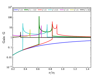
Figure 5: Spectral slices of the gain $G$ at a few observer locations for $a=60$ AU and ${\rm DM}=10$ pc cm^-3.

When a burst is multiply imaged and the extra delays in the arrival times of subimaged bursts are smaller than their widths, the subimages will interfere, producing time-frequency structure like that seen in the dynamic spectra of pulsars. Small lenses with $a\lesssim 1$ AU that yield sub-microsecond arrival time differences will produce frequency structure on scales of $\sim 1$ to 100 MHz. These oscillations will modulate the broader, caustic-induced frequency shape by amounts that depend on the gain ratio of a pair of images. If all three images contribute significantly, the oscillation frequencies $f_{ij}$ will satisfy a closure relation, $f^{-1}_{12}+f^{-1}_{23}+f^{-1}_{31}=0$. Measurements of oscillations can provide a test for the presence of multiple imaging.

2.7 Effects of Source Size and Motion

A change in the position of a point source alters the total phase $\Phi$ in the Kirchoff diffraction integral (Appendix A). Therefore, integrating over an extended source of size $\delta u_{\rm s}=\delta x_{\rm s}/a$ will reduce the gain if $\delta u_{\rm s}$ induces a phase shift $\sim\pi$. This translates into an upper bound on the source size,

$$\delta x_{\rm s}\leq\frac{a\pi}{\partial_{u_{\rm s}}\Phi} = \frac{\lambda d_{\rm sl}}{2a}\left(\frac{2u^{2}-1}{u}\right)\left(\frac{G}{G-1}\right)$$ (18)

$$\approx 3\times 10^{9}~{}{\rm cm}\,\frac{d_{\rm sl,{kpc}}}{a_{\rm AU}\nu},$$

where the approximate equality is for position and gain factors of order unity, an AU-size lens, and a source-lens distance $\sim 1$ kpc. Higher frequencies, larger lenses, and lenses nearer the source yield more stringent requirements on $\delta x_{\rm s}$.

The nominal upper bound on $\delta x_{\rm s}$ is similar to that required to see interstellar scintillations of Galactic pulsars and is easily satisfied by emission regions with transverse sizes of a light millisecond ($\sim 3\times 10^{7}$ cm). The light cylinder of a rotating object with period $P\lesssim 1$ s has radius $\sim 5\times 10^{9}P$ cm, so even slowly spinning objects with small emission regions inside their light cylinders will show lensing. Emission from larger objects, such as AGN jets will strongly attenuate the lensing unless there is coherent emission from very small substructures.

Relativistic beaming of radiation from the source could in principle reduce the illuminated portion of the lens, but the beam exceeds the lens size for $\gamma<2\times 10^{8}\,d_{\rm sl,{kpc}}/a_{\rm AU}$. This is well satisfied, for example, by relativistic flows in the magnetospheres of neutron stars for which radio emission is estimated to be from particles with $\gamma\lesssim 10^{3}$.

To calculate the time scale for changes in gain through caustics, we calculate the change in position on the screen $\delta u$ of a ray by taking the derivative of the lens equation Eq. 2 and employing other quantities,

$$\delta u=G\delta u^{\prime}=G\left[(d_{\rm lo}/d_{\rm so})\delta u_{\rm s}+(d_{\rm sl}/d_{\rm so})\delta u_{\rm obs}\right].$$ (19)

The corresponding change in gain is $\delta G\approx(dG/du)\delta u$, or

$$\frac{\delta G}{G}=\frac{4G(G-1)u(u^{2}-3/2)\delta u^{\prime}}{|1-2u^{2}|}.$$ (20)

Motions of source and observer combine into an effective transverse velocity,

$$v_{\perp}=(d_{\rm lo}/d_{\rm so})v_{\rm s,\perp}+(d_{\rm sl}/d_{\rm so})v_{\rm obs,\perp}.$$ (21)

Using $\delta u^{\prime}=v_{\perp}t_{\rm caustic}/a$ and $v_{\perp}=100\,v_{100}\,{\rm km~{}s}\,$, the characteristic time scale of a caustic crossing is

$$\!\!\!\!\!\!\!t_{\rm caustic}\sim\frac{a(\delta G/G)}{v_{\perp}G^{2}}\left(\frac{d_{\rm so}}{d_{\rm lo}}\right)\sim\frac{4.2\ {\rm hr}\times a_{\rm AU}(\delta G/G)}{v_{100}(G/10)^{2}}\left(\frac{d_{\rm so}}{d_{\rm lo}}\right).$$

(22)

The brightest caustics can yield $G>10$ and even smaller characteristic times.

The gain trough centered on $u^{\prime}=0$ has a width $\Delta u^{\prime}\sim 5$ (Figure 4), corresponding to a radio-dim time span,

$$t_{\rm trough}\sim\frac{a\Delta u^{\prime}}{v_{\perp}}\approx 87\,{\rm d}\left(\frac{a_{\rm AU}}{v_{100}}\right).$$ (23)

3 Single Lens Examples Relevant to FRBs

Our view is that multiple plasma lenses in the host galaxy of an FRB have a variety of dispersion depths, sizes, and distances from the source. Individually these will produce lensing effects that span a wide range of time scales, gains, and timing perturbations as described in the previous section. However, caustics may also result from the collective effects of two or more lenses and the duty cycle for lensing may be larger than implied for a single lens. A detailed analysis of multiple lenses is beyond the scope of the present paper.

For specificity, we consider a lens with a dispersion depth ${\rm DM}_{\ell}=10$ pc cm^-3 and scale size $a=60$ AU. These parameters, along with the same distance parameters as before ($d_{\rm so}=1$ Gpc and $d_{\rm sl}=1$ kpc), yield observables that are similar, at least qualitatively, to those seen for the repeating FRB121102. However, we emphasize that the observations do not allow any unique determination of parameter values and our choices here are simply for the purpose of illustration. A detailed comparison with the multiple bursts detected from the repeater FRB121102 will appear elsewhere.

The lens parameters give $\alpha=9.5\,\nu^{-2}$ and a focal frequency (Eq. 8) $\nu_{\rm f}\sim 2$ GHz comparable to typical observation frequencies used in FRB surveys.

Figure 6 shows the gains of individual subimages along with the total gain as a function of frequency for a particular location $u^{\prime}=2.2$. Gain enhancements are confined roughly to the frequency band of 1.28 to 1.78 GHz and appear as two caustic peaks, one rising at lower frequencies, the other rising at higher frequencies. The gain is suppressed below unity below the low-frequency caustic while it asymptotes to unity above the high-frequency caustic.

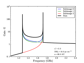
Figure 6: Gain vs. frequency for individual subimages and the summed gain at a selected transverse position $u^{\prime}=2.2$ and a lens with ${\rm DM}_{\ell}=10$ pc cm^-3 and $a=60$ AU.

Observations of FRB121102 have spanned $\sim 4$ yr to date and would correspond to a variation in $u^{\prime}$ that depends on the geometry and relevant transverse velocities, which are dominated by source or lens motions for lenses in host galaxies.

To compactly display the range of gains, arrival times, and dispersion measures of bursts, we show events in the frequency-$\delta$TOA plane in Figure 7 (left-hand panels) and in the frequency-DM plane (right-hand panels) color coded by $u^{\prime}$. By symmetry, we show results only for $u^{\prime}\geq 0$. The upper row shows all events with $G>5$ and the lower row with $G>20$. Many of the events in the upper row are cases with only one image or only one subimage above the gain threshold. However, there are many doublet cases where two events occur at the same frequency and location but arrive at different times. These are designated by black horizontal lines that connect the pair of events in each case. There is a smaller number of triplet cases, shown as red horizontal lines that connect black points. Most of the triplets occur near the focal frequency $\nu_{\rm f}\sim 2$ GHz and with arrival times shifted by $\lesssim 10$ ms. However, doublets occur over a broader range of arrival times up to 40 ms.

Over a range of epochs in which the $u^{\prime}$ prime plane is sampled, bright events will occur with arrival times and DMs that are perturbed by the plasma lens. Bright singlet events will cluster around an arrival time $\sim 1$ ms and ${\rm DM}\sim 2$ pc cm^-3. Multiplet bursts occuring at the same epoch will have slightly different arrival times and dispersion measures, with spreads up to a few milliseconds and a few $\times$ pc cm^-3.

For the particular lens and geometry considered here as an example, FRBs having intrinsically single component widths $W\sim 1$ to 8 ms will appear as blends of two or three subcomponents when they are imaged as multiplets. Triplets in some cases may appear as distinct subcomponents with little or no overlap and slightly different DMs.

For comparison we also considered a smaller lens with smaller dispersion depth that has a larger focal frequency. This case yields smaller perturbations of arrival times and burst DMs. Delays are $\lesssim 1~{}\mu$s at 1 GHz and differential TOAs between multiply-imaged bursts $\lesssim 0.1~{}\mu$s can produce frequency structure in the radio spectrum on the scale of tens to hundreds of MHz.

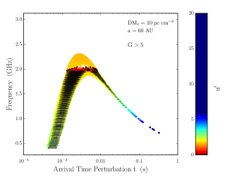
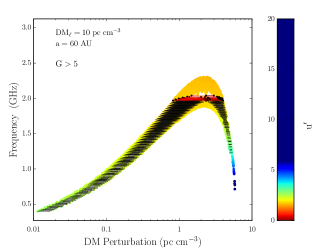
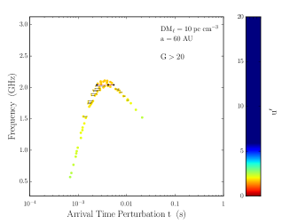
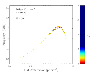
Figure 7: Frequencies, arrival times, and dispersion measures of bursts. Points are shown from locations across the transverse plane $u^{\prime}$ if they exceed a minimum gain. Top row: gains $>5$. Bottom row: gains $>20$. The left-hand panels show burst frequencies and arrival times. The right-hand panels show burst frequencies and dispersion measures. The locations of points in the $u^{\prime}$ plane are color coded according to the color bar. Only points with $u^{\prime}\geq 0$ are shown. Black horizontal lines designate ‘doublets’ with the same $\nu$ and $u^{\prime}$ that both exceed the minimum gain but differ in arrival time and DM. Triplets are shown as red horizontal lines connecting three black points.

4 Filaments in the Crab Nebula

Here we consider the effects of the Crab Nebula on measured pulses from the Crab pulsar because they demonstrate the overall approach taken in this paper.

Backer et al. (2000) and Graham Smith et al. (2011) reported transient echoes of radio pulses from the Crab pulsar that they attributed to plasma lensing like that described in Clegg et al. (1998). The filaments causing the echoes have estimated radii $\sim 1$ AU and dispersion depths ${\rm DM}_{\ell}\sim 0.1$ pc cm^-3.

At 1 GHz the implied lens parameter for a pulsar-lens distance $d_{\rm sl}=1$ pc and a pulsar-Earth distance $d_{\rm so}=2$ kpc is $\alpha\sim 0.34\,{d_{\rm sl}}_{\rm pc}a_{\rm AU}^{2}({\rm DM}_{\ell}/0.1~{}{\rm pc~{}cm^{-3}})$ corresponding to a focal distance $d_{\rm f}\sim 13$ kpc, well beyond the Crab pulsar’s distance. However, Graham Smith et al. (2011) use the duration of the ‘shadow’ region where the flux density is suppressed to estimate the size of the lens. Inspection of Figures 3 and 4 indicates that the half width of the shadow region is about twice the lens radius (which is unity in normalized coordinates), so the filaments are a factor of two smaller, leading to a focal distance $\sim 3$ kpc at 1 GHz. At the observation frequencies $\nu=0.33$ and 0.61 GHz where echoes were prominent, the focal distances are then 0.35 and 1.2 kpc, consistent with plasma lensing as the cause of the echoes because the Earth is then beyond the focal point and the criterion in Eq. 9 is met.

Compared to the filaments causing radio echoes, optical filaments in the Crab Nebula have larger scales extending to 2000 AU (Davidson & Fesen, 1985) and potentially large ${\rm DM}_{\ell}$, giving much larger focal distances, $d_{\rm f}\sim 0.52\,{\rm Gpc}\,(10~{}{\rm pc~{}cm^{-3}}/{\rm DM}_{\ell})(a/2000~{}{\rm AU})^{2}$. This suggests that compact objects in extragalactic supernova remnants may show lensing from similar structures. If lensing is required for detection of FRBs, particular scale sizes and electron densities will be selected as a function of true source distance. Equivalently, if burst sources reside in supernova remnants of similar age and other properties, nearby sources will be selected against if they are closer than the focal distance because lensing will not enhance their flux densities.

5 Plasma Lenses in Host Galaxies

While the IGM provides long path lengths through ionized gas, there is no indication that it harbors small scale structures (e.g. 1 to 1000 AU). However, host galaxies of FRBs almost certainly have plasma structures similar to those inferred to be present in the ISM of the Milky Way. We therefore consider plasma lenses in host galaxies. Our treatment is for Euclidean space (i.e. low redshifts) because the main points can be made in this regime and the best studied source to date, FRB121102, is at a low redshift $z\sim 0.193$ (Tendulkar et al., 2017).

Several cases may be considered that represent a large range of possible scale sizes and dispersion-measure depths but together can give similar values of $\alpha$ (Eq. 3) and hence the same focal distances and focal frequencies defined earlier.

One possibility comprises a bow shock produced by an FRB source moving in a dense medium; the source-lens distance is then quite small, $d_{\rm sl}\lesssim 1$ pc. In this case the FRB source directly influences its plasma environment. However, the relative velocity between the bow shock and the source is small unless clumps form in the rapidly moving flow along the bow shock.

A second case is an FRB source enclosed by a supernova remnant (SNR) of $\sim$pc radius. This would satisfy Eq. 7 with small knots or filaments within the shell that provide DM$\sim 1$ pc cm^-3 (after accounting for any redshift dependences). Among SNRs, we expect diverse properties of ionized gas clumps that depend on the masses of progenitors and on the details of pre-supernova mass loss.

A third possibility is that larger structures, such as HII regions, with larger ${\rm DM}_{\ell}$ and larger (e.g. kpc) distances from the source provide the lensing structures. These would clearly be uninfluenced by the FRB source. This case may rely on a fortuitious alignment of the lenses with the source while the other options involve direct coupling of the source and the lensing region. However, FRBs may reside in galaxies where such alignments are not improbable.

To assess the above three cases we require that the source and lens be further than the focal distance (i.e. $d_{\rm f}\leq d_{\rm so}$). Using Eq. 7 and expressing ${\rm DM}_{\ell}=an_{\rm e}$ in terms of the electron density $n_{\rm e}=10^{4}n_{\rm e_{4}}$ cm^-3, we get

$$a\leq\frac{r_{\rm e}c^{2}}{\pi\alpha_{\rm min}}\frac{d_{\rm sl}n_{\rm e}}{\nu^{2}}=74~{}{\rm AU}\times\frac{n_{\rm e_{4}}d_{\rm sl,{kpc}}}{\nu^{2}}.$$ (24)

Lenses at $\sim$kpc distances can be much larger and provide more gain, but still require large electron densities. However, lenses within 1 pc of the source must be very small ($\lesssim 0.1$ AU) or the electron density very high ($>10^{4}$ cm^-3) for larger lenses to provide strong lensing effects. Small lenses provide less gain than larger lenses because the maximum gain $\propto a$ scales as the one-dimensional ‘area.’

Additional constraints may allow us to favor lenses near or far from a source (but still in the host galaxy). Higher gain lenses will show more rapid variability (Eq. 22), all else being equal, because the caustic time scale $t_{\rm caustic}\propto G^{-1}$ if the maximum gain $G_{\rm max}\propto a$ is substituted.

The emission measure,

$${\rm EM}=an_{\rm e}=485~{}{\rm pc~{}cm^{-6}}a_{\rm AU}n_{\rm e_{4}}^{2},$$ (25)

yields free-free absorption with an optical depth at $\nu$ in GHz (Draine, 2011),

$$\tau_{\rm ff}\approx 3.4\times 10^{-7}\nu^{-2.1}T_{4}^{-1.32}{\rm EM}.$$ (26)

The focusing constraint in Eq. 24 implies an upper bound on EM and the optical depth,

$${\rm EM}\lesssim 3.59\times 10^{4}~{}{\rm pc~{}cm^{-3}}\times\frac{n_{\rm e_{4}}^{3}d_{\rm sl,{kpc}}}{\nu^{2}}$$ (27)

and

$$\tau_{\rm ff}\lesssim 0.12\times\frac{n_{\rm e_{4}}^{3}d_{\rm sl,{kpc}}}{\nu^{2}}.$$ (28)

Free-free absorption can be important at GHz frequencies for lenses at $d_{\rm sl}\sim 1$ kpc with densities $\sim 5\times 10^{4}$ cm^-3 but smaller source-lens distances require significantly higher densities.

The large implied electron density in all cases gives a large over pressure ${\cal P}=n_{\rm e}kT$ compared to typical ISM values, identical to the same overpressure identified for Galactic ESEs (e.g. Bannister et al., 2016). The magnetic field that could confine lenses with temperature $T=10^{4}T_{4}$ is

$$B=\left(8\pi n_{e}kT\right)^{1/2}\sim 0.59~{}{\rm mG}\left(n_{\rm e_{4}}T_{4}\right)^{1/2}$$ (29)

implying a maximum Faraday rotation measure (when the parallel magnetic field is along the line of sight without any reversals),

$${\rm RM}_{\rm max}\sim 24\,{\rm rad~{}m^{-2}}\,a_{\rm AU}n_{\rm e_{4}}^{3/2}T_{4}^{1/2}.$$ (30)

As yet there is insufficient information to favor lenses for the repeating FRB that are at distances from the source of pc or kpc (or something in between). Wideband spectra and more complete sampling of periods of high gain can constrain the lens size and dispersion measure depth.

6 Summary and Conclusions

In this paper we have shown that small, one-dimensional plasma lenses with small dispersion depths can strongly amplify radio bursts emitted at Gpc distances. Filamentary structures seen in the Crab Nebula, timing variations of the Crab pulsar and a few other pulsars, and extreme lensing events in AGN light curves demonstrate that AU-size structures with high electron densities exist in the Milky Way. Presumably they also exist in the ionized gas in FRB host galaxies. Recent work (Metzger et al., 2017; Beloborodov, 2017) has made the compelling case that FRBs are associated with young, rapidly spinning magnetars. These objects dissipate much more energy into their environment than the Crab pulsar and therefore can be expected to drive shocks into presupernova wind material that may fragment into lensing structures.

In this paper we analyzed the properties of individual plasma lenses with Gaussian density profiles and identified some key features. Gaussian plasma lenses yield both amplification and suppression of the apparent burst flux densities in a time sequence as follows. The gain is initially unity for lines of sight far from the lens. As the line of sight nears the lens, a short duration, large amplitude spike ($\sim 1~{}$d) occurs followed by a long-duration ($\sim$months) trough of low gain that can be much less than unity. Another caustic spike is then encountered that asymptotes to the quiescent state as the line of sight moves away from the lens. These time scales can be larger or smaller depending on the size of the lens and on the effective velocity by which the geometry changes.

As a function of frequency, the gain pattern suppresses all frequencies in the trough but shows asymmetric, large amplitude cusps at epochs where a source is multiply imaged. Burst spectra can therefore show narrow structure even if the intrinsic spectrum is smooth.

Gaussian density profiles produce multiply imaged bursts with different apparent strengths, arrival times, and dispersion measures. The frequency dependence of arrival times can differ markedly from the $\nu^{-2}$ scaling of cold plasma dispersion. If arrival times of individual bursts are fitted with a $\nu^{-2}$ scaling law, negative dispersion measure perturbations will be obtained at some epochs (which, of course, add to a much larger DM through the remainder of the host galaxy, the IGM, and the Galaxy). When subimages are comparable in strength, burst spectra may also show oscillations due to interference between subimages if their arrival time difference is smaller than the burst width. Arrival time perturbations from lenses, whether for a singly imaged or multiply imaged burst, can be large enough to mask any underlying periodicity with period much less than one second.

Detection of bursts in large-scale surveys may rely on the presence of spectral caustics, which can elevate the apparent flux density by factors up to $\sim 100$. Followup observations, in turn, may be deleteriously affected by the gain trough that will follow a caustic spike. The actual amount of amplification is larger for larger lenses and will be attenuated for sources larger than about $10^{10}$ cm for nominal parameters. Any scattering from additional electron density fluctuations in the lens or between the source and lens can also attenuate the amplification.

Many of the phenomena observed from the repeating FRB121102 are consistent, at least qualitatively, with the features we have derived for the Gaussian lens. These, in turn, are expected to be generic for lenses with non-Gaussian column density profiles because they result primarily from the presence of inflection points in the total phase (geometric + dispersive). Non-Gaussian lenses will share some of these properties but likely will not be symmetric nor do we expect the specific details of cusps in the spectra or light curves of radio sources to be the same.

Testing of the lensing interpretation of the intermittency of FRB121102 (and other FRB sources if they actually repeat) can proceed in several ways, including the measurement of very wideband spectra covering many octaves, e.g. 0.4 to 20 GHz. These can identify the pairs of caustic spikes expected from a single Gaussian lens or, perhaps, multiple spikes for more complicated lensing structures. If such spectra are obtained with high spectral resolution ($<1$ MHz), oscillations from interference between subimages may also be detected in frequency ranges containing caustic spikes.

A detailed discussion of individual bursts from FRB121102, including an interpretation in terms of lensing, will be given in papers by J. Hessels et al. (in preparation) and C. Law et al. (in preparation). Further study of lensing that include two dimensional lenses and the effects of multiple lenses is also in progress.

A related analysis should be made of Galactic lenses to address why only modest lensing gains have been identified (so far) from Galactic sources. It is possible that most Galactic lenses have very small or very large focal distances that are selected against. Radio wave scattering from the general ISM may also mask or attenuate strong lensing.

Acknowledgements:

We thank Laura Spitler for useful correspondence and conversations. S.C. and J.M.C., are partially supported by the NANOGrav Physics Frontiers Center (NSF award 1430284). Work at Cornell (J.M.C., S.C., R.S.R. ) was supported by NSF grants AST-1104617 and AST-1008213. J.W.T.H. acknowledges funding from an NWO Vidi fellowship and from the European Research Council under the European Union’s Seventh Framework Programme (FP/2007-2013) / ERC Starting Grant agreement nr. 337062 (”DRAGNET”). I. W. was supported by National Science Foundation Grant Phys 1104617 and National Aeronautics and Space Administration grant NNX13AH42G. Part of this research was carried out at the Jet Propulsion Laboratory, California Institute of Technology, under a contract with the National Aeronautics and Space Administration.

Appendix A Kirchhoff Diffraction Integral (KDI) for the Gaussian Plasma Lens

We use dimensionless coordinates $u$, $u_{\rm s}$, $u^{\prime}$ defined in the main text and $u_{\rm F}$, the normalized Fresnel scale ($r_{\rm F}$),

$$u_{\rm F}=\frac{r_{\rm F}}{a}=\frac{1}{a}\left(\frac{\lambda d_{\rm sl}d_{\rm lo}}{2\pi d_{\rm so}}\right)^{1/2}.$$ (A1)

The scalar field from the KDI is

$$\varepsilon(u^{\prime}) = \frac{1}{u_{\rm F}\sqrt{2\pi i}}\int du\,\exp\left[{i\Phi(u,u_{\rm s},u_{\rm obs})}\right],$$ (A2)

where the total phase is

$$\Phi(u,u_{\rm s},u_{\rm obs}) = \left(2u_{\rm F}^{2}\right)^{-1}\left[(d_{\rm lo}/d_{\rm so})(u-u_{\rm s})^{2}+(d_{\rm sl}/d_{\rm so})(u-u_{\rm obs})^{2}-(d_{\rm sl}d_{\rm lo}/d_{\rm so}^{2})(u_{\rm obs}-u_{\rm s})^{2}\right]+\phi_{\rm lens}(u)$$ (A3)

and $\phi_{\rm lens}(u)$ is the phase perturbation from the lens. The KDI is normalized so that without a screen ($\phi_{\rm lens}=0$), the intensity $|\varepsilon(u^{\prime})|^{2}=1$. The lens equation in Eq. 2 (main text) is the stationary phase (SP) solution given by $\partial_{u}\Phi(u,u_{\rm s},u_{\rm obs})=0$ where $\partial_{u}\equiv\partial/\partial u$.

The geometrical optics gain $G$ (Eq. 4) results from expanding the phase to second order about a particular SP solution $\overline{u}$, $\Phi(u)\approx\Phi(\overline{u},u_{\rm s},u_{\rm obs})+(1/2)\partial_{u}^{2}\Phi(\overline{u},u_{\rm s},u_{\rm obs})(u-\overline{u})^{2}$ and taking the squared magnitude of the resulting integral. We define $G$ to be $\geq 0$ but also define the parity of the integral as the sign of the second derivative, which changes at the inflection point of the total phase.

When the geometrical optics gain diverges, higher order terms in the phase expansion (or the exact phase) are needed to properly calculate the gain. Numerical and analytical results indicate that for $G\to\infty$, the physical optics gain is given for most $\overline{u}$ by using the additional cubic term $(1/6)\partial_{u}^{3}\Phi(\overline{u},u_{\rm s},u^{\prime})(u-\overline{u})^{3}$ in the KDI, which yields the analytical result,

$$G_{\rm p_{3}}\approx\frac{6^{2/3}2}{9\pi}\left[\frac{\Gamma(1/3)\cos\pi/6}{|\partial_{u}^{3}\Phi(\overline{u},u_{\rm s},u_{\rm obs})|^{1/3}}\right]^{2}.$$ (A4)

If $\partial_{u}^{3}\Phi$ has any zeros in $u$, higher-order terms are needed.

For the Gaussian lens, $\phi_{\rm lens}(u)=-\lambda r_{\rm e}{\rm DM}_{\ell}e^{-u^{2}}=-(\alpha/2u_{\rm F}^{2})e^{-u^{2}}$. The geometrical optics gain is

$$G=|1+\alpha(1-2u^{2})e^{-u^{2}}|^{-1}.$$ (A5)

At inflection points where $G\to\infty$, $G_{\rm p_{3}}$ is calculated instead by substituting the third derivative $\partial_{u}^{3}\Phi(\overline{u},u_{\rm s},u_{\rm obs})=4u_{\rm F}^{-2}\alpha\overline{u}e^{-\overline{u}^{2}}(\overline{u}^{2}-3/2)$ into Eq. A4. The approximation is good except at or near $\overline{u}=\sqrt{3/2}$ where $G_{\rm p_{3}}$ diverges. In that case we evaluate the KDI to obtain a finite value for the physical optics gain, $G_{\rm p}(\overline{u}=\sqrt{3/2})\sim u_{\rm F}^{-1}\propto a$ for $\alpha_{\infty}=e^{3/2}/2=2.24$. We note that for this case where $\overline{u}=\sqrt{3/2}$, the KDI is oscillatory because this location with $\alpha=\alpha_{\infty}$ produces an optical catastrophe (e.g. Berry & Upstill, 1980).

References

- Backer et al. (2000) Backer, D. C., Wong, T., & Valanju, J. 2000, ApJ, 543, 740
- Bannister et al. (2016) Bannister, K. W., Stevens, J., Tuntsov, A. V., et al. 2016, Science, 351, 354
- Beloborodov (2017) Beloborodov, A. M. 2017, ArXiv e-prints
- Berry & Upstill (1980) Berry, M., & Upstill, C. 1980, in Progress in Optics, Vol. 18, {IV} Catastrophe Optics: Morphologies of Caustics and Their Diffraction Patterns, ed. E. Wolf (Elsevier), 257 – 346
- Chatterjee et al. (2017) Chatterjee, S., Law, C. J., Wharton, R. S., et al. 2017, ArXiv e-prints
- Clegg et al. (1998) Clegg, A. W., Fey, A. L., & Lazio, T. J. W. 1998, ApJ, 496, 253
- Coles et al. (2015) Coles, W. A., Kerr, M., Shannon, R. M., et al. 2015, ApJ, 808, 113
- Connor et al. (2016) Connor, L., Sievers, J., & Pen, U.-L. 2016, MNRAS, 458, L19
- Cordes & Lazio (2002) Cordes, J. M., & Lazio, T. J. W. 2002, ArXiv Astrophysics e-prints
- Cordes & Wasserman (2016) Cordes, J. M., & Wasserman, I. 2016, MNRAS, 457, 232
- Davidson & Fesen (1985) Davidson, K., & Fesen, R. A. 1985, ARA&A, 23, 119
- Draine (2011) Draine, B. T. 2011, Physics of the Interstellar and Intergalactic Medium (Princeton University Press)
- Fiedler et al. (1987) Fiedler, R. L., Dennison, B., Johnston, K. J., & Hewish, A. 1987, Nature, 326, 675
- Graham Smith et al. (2011) Graham Smith, F., Lyne, A. G., & Jordan, C. 2011, MNRAS, 410, 499
- Heiles (1997) Heiles, C. 1997, ApJ, 481, 193
- Jenkins & Tripp (2011) Jenkins, E. B., & Tripp, T. M. 2011, ApJ, 734, 65
- Marcote et al. (2017) Marcote, B., Paragi, Z., Hessels, J. W. T., et al. 2017, ApJ, 834, L8
- Metzger et al. (2017) Metzger, B. D., Berger, E., & Margalit, B. 2017, ArXiv e-prints
- Pen & Connor (2015) Pen, U.-L., & Connor, L. 2015, ApJ, 807, 179
- Pen & Levin (2014) Pen, U.-L., & Levin, Y. 2014, MNRAS, 442, 3338
- Rickett (1990) Rickett, B. J. 1990, ARA&A, 28, 561
- Romani et al. (1987) Romani, R. W., Blandford, R. D., & Cordes, J. M. 1987, Nature, 328, 324
- Scholz et al. (2016) Scholz, P., Spitler, L. G., Hessels, J. W. T., et al. 2016, ArXiv e-prints
- Spitler et al. (2014) Spitler, L. G., Cordes, J. M., Hessels, J. W. T., et al. 2014, ApJ, 790, 101
- Spitler et al. (2016) Spitler, L. G., Scholz, P., Hessels, J. W. T., et al. 2016, Nature, 531, 202
- Tendulkar et al. (2017) Tendulkar, S. P., Bassa, C. G., Cordes, J. M., et al. 2017, ApJ, 834, L7
- Thornton et al. (2013) Thornton, D., Stappers, B., Bailes, M., et al. 2013, Science, 341, 53
- Tuntsov et al. (2016) Tuntsov, A. V., Walker, M. A., Koopmans, L. V. E., et al. 2016, ApJ, 817, 176
- Walker & Wardle (1998) Walker, M., & Wardle, M. 1998, ApJ, 498, L125
- Yao et al. (2016) Yao, J. M., Manchester, R. N., & Wang, N. 2016, ArXiv e-prints