Quantized Output Feedback Stabilization by Luenberger Observers

Abstract

We study a stabilization problem for systems with quantized output feedback. The state estimate from a Luenberger observer is used for control inputs and quantization centers. First we consider the case when only the output is quantized and provide data-rate conditions for stabilization. We next generalize the results to the case where both of the plant input and output are quantized and where controllers send the quantized estimate of the plant output to encoders as quantization centers. Finally, we present the numerical comparison of the derived data-rate conditions with those in the earlier studies and a time response of an inverted pendulum.

1 Introduction

Control loops in a practical network contain channels over which only a finite number of bits can be transmitted. Due to such limited transmission capacity, we should quantize data before sending them out through a network. However, large quantization errors lead to the deterioration of control performance. One way to reduce quantization errors under data-rate constraints is to exploit output estimates as quantization centers. In this paper, we adopt Luenberger observers as output estimators due to their simple structure and aim to design an encoding strategy for stabilization.

A fundamental limitation of data rate for stabilization was first obtained by Wong and Brockett (1999), and inspired by this result, data-rate limitations were studied for linear time-invariant systems in Tatikonda and Mitter (2004), for stochastic systems in Nair and Evans (2004), and for uncertain systems in Okano and Ishii (2014). Although the so-called zooming-in and zooming-out encoding method developed in Brockett and Liberzon (2000); Liberzon (2003b) provides only sufficient conditions for stabilization, this encoding procedure is simple and hence was extended, e.g., to nonlinear systems in Liberzon and Hespanha (2005); Liberzon (2006), to systems with external disturbances in Liberzon and Nešić (2007); Sharon and Liberzon (2008, 2012), and recently to switched/hybrid systems in Liberzon (2014); Yang and Liberzon (2015); Wakaiki and Yamamoto (2016). Readers are referred to the survey papers by Nair et al. (2007); Ishii and Tsumura (2012), and the books by Matveev and Savkin (2009); Liberzon (2003c) on this topic for further information.

Although Luenberger observers has been widely used for quantized output feedback stabilization, e.g., in Liberzon (2003a); Ferrante et al. (2014); Xia et al. (2010), state estimates was exploited only to generate control inputs, and a quantization center was the origin. However, to reduce quantization errors, output estimates play an important role as quantization centers.

The notable exception is the studies by Sharon and Liberzon (2008, 2012). The class of observers in these studies covers a Luenberger observer whose estimate is initialized by a pseudo-inverse observer, and Sharon and Liberzon (2008, 2012) provided a sufficient condition for stabilization with unbounded disturbances. However, this condition is not easily verifiable for the case of Luenberger observers. Furthermore, these studies placed assumptions that input quantization is ignored and that encoders contain state estimators for sharing quantization centers with controllers.

In this paper, we present an output encoding method for the stabilization of sampled-data systems with discrete-time Luenberger observers. The proposed encoding method is based on the zooming-in technique and employs estimates generated from a Luenberger observer for both stabilization and quantization. First we consider only output quantization and assume that encoders also contain estimators. Simple sufficient conditions for stabilization are obtained in the both case of general Luenberger observers and of deadbeat observers.

Second we generalize the results of general Luenberger observers to the situation where both of the plant input and output are quantized. Moreover, in the second case, encoders do not estimate the plant state by themselves, but controllers send the quantized estimate of the plant output to the encoders. In contrast with the quantization of the plant output, we quantize the plant input and the output estimate by using the origin as the quantization center, which reduces computational resources in the components of the plant side. We see that if the closed-loop system without quantization is stable, then there exists an encoding method such that the closed-loop system in the presence of three types of quantization errors is also stable.

This paper is organized as follows. In the next section, we study the case when only the plant output is quantized and obtain two data-rate conditions for general Luenberger observers and deadbeat observers. In Section 3, the proposed encoding method is extended to the case when both of the plant input and output are quantized. Section 4 is devoted to the numerical comparison of the obtained data-rate conditions with those of the earlier studies by Liberzon (2003b); Sharon and Liberzon (2008, 2012) and the time response of an inverted pendulum. We provide concluding remarks in Section 5.

Notation and Definitions:

The symbol $\mathbb{Z}_{+}$ denotes the set of nonnegative integers. Let $\lambda_{\min}(P)$ and $r(P)$ denote the smallest eigenvalue and the spectral radius of $P\in\mathbb{R}^{\sf n\times n}$, respectively. For a vector $v=[v_{1}~{}\!\dotsb~{}\!v_{\sf n}]^{\top}\in\mathbb{R}^{\sf n}$, we denote its maximum norm by $|v|=\max\{|v_{1}|,\dots,|v_{\sf n}|\}$ and the corresponding induced norm of a matrix $M\in\mathbb{R}^{\sf m\times n}$ by

$$\|M\|=\sup\{|Mv|_{\infty}:~{}v\in\mathbb{R}^{\sf n},~{}|v|_{\infty}=1\}.$$

Plant:

We consider a continuous-time linear system

$$\Sigma_{P}:\begin{cases}\begin{aligned} \dot{x}(t)&=Ax(t)+Bu(t)\\ y(t)&=Cx(t),\end{aligned}\end{cases}$$ (1)

where $x(t)\in\mathbb{R}^{\sf{n}}$ is the state, $u(t)\in\mathbb{R}^{\sf{m}}$ is the control input, and $y(t)\in\mathbb{R}^{\sf{p}}$ is the output. This plant is connected with a controller through a time-driven encoder and zero-order hold (ZOH) with period $h>0$. Define

$$x_{k}:=x(kh),\qquad y_{k}:=y(kh)$$

for every $k\in\mathbb{Z}_{+}$, and also set

$$A_{d}:=e^{Ah},\qquad B_{d}:=\int^{h}_{0}e^{As}Bds.$$ (2)

Throughout this paper, we place the following assumptions:

Assumption 1 (Initial state bound)

A constant $E_{st}>0$ satisfying $|x(0)|\leq E_{st}$ is known.

Assumption 2 (Stabilizability and detectability)

The discretized system $(A_{d},B_{d},C)$ is stabilizable and detectable.

Remark 3

We can obtain an initial state bound $E_{st}$ by the “zooming-out” procedure in Liberzon (2003b).

2 Output Quantization

In this section, we consider the scenario where only the output $y_{k}$ is quantized and where the encoder has computational resources to estimate the plant state.

2.1 Controller

Let $q_{k}\in\mathbb{R}^{\sf{p}}$ be the quantized value of the sampled output $y_{k}$ and $K\in\mathbb{R}^{\sf{n}\times\sf{m}},L\in\mathbb{R}^{\sf{n}\times\sf{p}}$ be a feedback gain and an observer gain, respectively. For the plant $\Sigma_{P}$ in (1), we use a discrete-time Luenberger observer for feedback control and output quantization:

$$\Sigma_{C}:\begin{cases}\begin{aligned} \hat{x}_{k+1}&=A_{d}\hat{x}_{k}+B_{d}u_{k}+L(q_{k}-\hat{y}_{k})\\ \hat{y}_{k}&=C\hat{x}_{k}\\ u_{k}&=-K\hat{x}_{k}\end{aligned}\end{cases}$$ (3)

where $\hat{x}_{k}\in\mathbb{R}^{\sf{n}}$ is the state estimate and $\hat{y}_{k}\in\mathbb{R}^{\sf{p}}$ is the output estimate. We set the initial estimate $\hat{x}_{0}$ to be $\hat{x}_{0}=0$. Each of the encoder and the controller contains the above Luenberger observer, and those observers are assumed to be synchronized. Through the zero-order hold, the control input $u(t)$ is generated as

$$u(t)=u_{k}\qquad(kh\leq t<(k+1)h).$$

Fig. 1 shows the closed-loop system with quantized output.

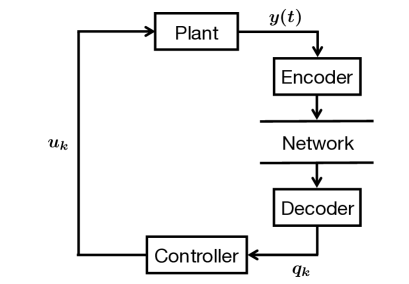
Figure 1: Closed-loop system with output quantization.

2.2 Output Encoding

Suppose that we obtain an error bound $E_{k}$ such that $|y_{k}-\hat{y}_{k}|\leq E_{k}$. The next subsection is devoted to the computation of a bound sequence $\{E_{k}\}$ for stabilization.

For each $k\in\mathbb{Z}_{+}$, we divide the hypercube

$$\left\{y\in\mathbb{R}^{\sf p}:~{}|y-\hat{y}_{k}|_{\infty}\leq E_{k}\right\}$$ (4)

into $N^{\sf p}$ equal boxes and assign a number in $\{1,\dots,N^{\sf p}\}$ to each divided box by a certain one-to-one mapping. Since $\hat{x}_{0}=0$, we see from Assumption 1 that the error $e_{k}:=x_{k}-\hat{x}_{k}$ satisfies $|e_{0}|=|x(0)|\leq E_{st}$. Thus we can set

$$E_{0}:=\|C\|E_{st}.$$

The encoder sends to the controller the number $\bar{q}_{k}$ of the divided box containing $y_{k}$, and then the controller generates $q_{k}$ equal to the center of the box with number $\bar{q}_{k}$. If $y_{k}$ lies on the boundary on several boxes, then we can choose any one of them. This encoding strategy leads to

$$|y_{k}-q_{k}|\leq\frac{E_{k}}{N}=:\mu_{k}.$$ (5)

2.3 Computation of Bound Sequence $\{E_{k}\}$

Here we obtain bound sequences $\{E_{k}\}$ and data-rate conditions for stabilization. We first consider general Luenberger observers and next focus on deadbeat observers.

2.3.1 Use of General Luenberger Observers:

The proposed encoding strategy with the following bound sequence $\{E_{k}\}$ achieves the exponential convergence of the state under a certain data-rate condition.

Theorem 4

Let Assumptions 1 and 2 hold. Define the matrices $R$ and $\bar{R}$ by

$$R:=A_{d}-LC,\qquad\bar{R}:=A_{d}-B_{d}K.$$ (6)

Let the observer gain $L$ and the feedback gain $K$ satisfy $r(R)<1$, $r(\bar{R})<1$, and

$$\left\|CR^{\ell}\right\|\leq M_{0}\rho^{\ell},\quad\left\|CR^{\ell}L\right\|\leq M\rho^{\ell}.$$ (7)

for some $M_{0},M>0$ and $\rho<1$. If we pick $N\geq 2$ so that

$$\frac{M}{1-\rho}　<N,$$ (8)

then the proposed encoding method with a bound sequence $\{E_{k}\}$ defined by

$$E_{k+1}:=\begin{cases}M_{0}E_{st}\rho+\frac{M}{N}E_{0}&k=0\\ \left(\rho+\frac{M}{N}\right)E_{k}&k\geq 1.\end{cases}$$ (9)

achieves the exponential convergence of the state $x$ and the estimate $\hat{x}$.

The proof consists of two steps:

• Obtain the error bound $E_{k+1}$ from $E_{0},\dots,E_{k}$.

• Show state convergence.

We break the proof of Theorem 4 into the above two steps.

1) First we obtain an error bound $E_{k+1}$ for every $k\geq 0$ under the assumption that $\mu_{0},\dots,\mu_{k}$ are obtained.

Since the estimation error $e_{k}=x_{k}-\hat{x}_{k}$ satisfies

$$e_{k+1}=Re_{k}+L(y_{k}-q_{k}),$$ (10)

and hence

$$e_{k+1}=R^{k+1}e_{0}+\sum^{k}_{\ell=0}R^{\ell}L(y_{k-\ell}-q_{k-\ell}).$$ (11)

Define $E_{k+1}$ by

$$E_{k+1}:=M_{0}E_{st}\rho^{k+1}+M\sum_{\ell=0}^{k}\rho^{\ell}\mu_{k-\ell}$$ (12)

for every $k\geq 0$. Then we conclude from (11) that

$$|y_{k+1}-\hat{y}_{k+1}|\leq E_{k+1}.$$ (13)

Moreover, from (12), we see that

$$E_{k+1}-\rho E_{k}=\frac{M}{N}E_{k}$$

for every $k\geq 1$, and hence (9) is obtained. Thus if (8) holds, then $E_{k}$ and $\mu_{k}=E_{k}/N$ exponentially converge to zero. $\blacksquare$ and hence

$$|y_{k+1}-q_{k+1}|\leq\frac{E_{k+1}}{N}.$$ (14)

By definition, $\mu_{k}=E_{k}/N$ satisfies

$$\mu_{k+1}-\rho\mu_{k}=\frac{M}{N}\mu_{k},$$

and hence

$$\mu_{k+1}=\left(\frac{M}{N}+\rho\right)\mu_{k}.$$

Thus if (8) holds, then $\mu_{k}$ exponentially converges to zero.

2) Using the convergence of $\mu$, we next show the state convergence. For every $k\geq 0$, $\mu_{k}$ satisfies $\mu_{k}\leq\widetilde{\mu}_{0}\widetilde{\rho}^{k}$, where $\widetilde{\rho}:=M/N+\rho<1$ and $\widetilde{\mu}_{0}:=\max\{\mu_{0},\mu_{1}/\widetilde{\rho}\}$. Then, from (5) and (11), we have some constant $M_{e}>0$ satisfying $|e_{k}|<M_{e}\widetilde{\mu}_{0}\widetilde{\rho}^{k}$ for all $k\geq 0$. Here we used $\|C\|\cdot|e_{0}|\leq E_{0}=N\mu_{0}\leq N\widetilde{\mu}_{0}$.

Since $\bar{R}=A_{d}-B_{d}K$ is Schur stable, there exist a positive scalar $c$ and a positive definite matrix $P$ such that

$$\bar{R}^{\top}P\bar{R}-P\leq-cP.$$

Since

$$x_{k+1} =A_{d}x_{k}-B_{d}K\hat{x}_{k}=\bar{R}x_{k}+B_{d}Ke_{k},$$ (15)

it follows that

$$V(x_{k+1})\!-\!V(x_{k}) \!\leq\!-cV(x_{k})\!+\!2\|K^{\top}B_{d}^{\top}P\bar{R}\|_{2}\!\cdot\!|x_{k}|_{2}\!\cdot\!|e_{k}|_{2}$$

$$\qquad+\!\|K^{\top}B_{d}^{\top}PB_{d}K\|_{2}\!\cdot\!|e_{k}|_{2}^{2}.$$

Young’s inequality leads to

$$2|x_{k}|_{2}\cdot|e_{k}|_{2}\leq\frac{1}{\theta}|x_{k}|_{2}^{2}+\theta|e_{k}|_{2}^{2}$$

for all $\theta>0$, and hence

$$V(x_{k+1})\leq\omega V(x_{k})+\bar{M}_{e}|e_{k}|_{2}^{2},$$ (16)

where

$$\omega :=1-c+\frac{\|K^{\top}B_{d}^{\top}P\bar{R}\|_{2}}{\theta\lambda_{\min}(P)}$$ (17)

$$\bar{M}_{e} :=\theta\|K^{\top}B_{d}^{\top}P\bar{R}\|_{2}+\|K^{\top}B_{d}^{\top}PB_{d}K\|_{2}.$$

We choose a sufficiently large $\theta>0$ so that $\omega<1$.

Since (16) leads to

$$V(x_{k+1})\leq\omega^{k+1}V(x_{0})+\bar{M}_{e}\sum_{\ell=0}^{k}\omega^{k-\ell}|e_{\ell}|^{2}_{2}$$

and since $|e_{k}|_{2}\leq\sqrt{\sf n}|e_{k}|\leq\sqrt{\sf n}M_{e}\widetilde{\mu}_{0}\widetilde{\rho}^{k}$, we obtain

$$V(x_{k+1})\leq\omega^{k+1}V(x_{0})+{\sf n}\bar{M}_{e}(M_{e}\widetilde{\mu}_{0})^{2}\sum_{\ell=0}^{k}\omega^{k-\ell}\widetilde{\rho}^{2\ell}.$$

If $\omega\not=2\widetilde{\rho}$, then

$$\sum_{\ell=0}^{k}\omega^{k-\ell}\widetilde{\rho}^{2\ell}\leq\frac{\omega^{k+1}-\widetilde{\rho}^{2(k+1)}}{\omega-\widetilde{\rho}^{2}}$$

otherwise,

$$\sum_{\ell=0}^{k}\omega^{k-\ell}\widetilde{\rho}^{2\ell}\leq(k+1)\omega^{k}.$$

For every $\widetilde{\omega}$ with $\widetilde{\omega}>\omega$, there exists a constant $M_{\tilde{\omega}}>0$ such that $M_{\tilde{\omega}}\widetilde{\omega}^{k}>k\omega^{k}$. We therefore have

$$|x_{k}|\leq M_{x}\widetilde{\mu}_{0}\gamma^{k}$$

for some $M_{x}>0$, where $\gamma:=\max\{\widetilde{\omega}/2,\widetilde{\rho}\}$. Here we again used $\|C\|\cdot|x_{0}|\leq N\widetilde{\mu}_{0}$. Hence $\hat{x}_{k}$ satisfies

$$|\hat{x}_{k}|\leq|x_{k}|+|e_{k}|\leq M_{\hat{x}}\widetilde{\mu}_{0}\gamma^{k}$$

for some $M_{\hat{x}}>0$.

Finally, $x$ satisfies

$$\dot{x}(t)=Ax(t)-BK\hat{x}_{k}$$

for all $t\in[kh,(k+1)h)$. From this linearity, there exists $M>0$ such that

$$|x(t)|\leq M\widetilde{\mu}_{0}e^{-\sigma t},$$

where $\sigma:=1/(2h)\cdot\log(1/\gamma)$. This completes the proof.

2.3.2 Use of Deadbeat Observers:

In the rest of this section, we focus on deadbeat observers. If the pair $(C,A_{d})$ is observable, then there exists a matrix $L\in\mathbb{R}^{{\sf n}\times{\sf p}}$ such that

$$R^{\eta}=(A_{d}-LC)^{\eta}=0,$$ (18)

where $\eta$ is the observability index of $(C,A_{d})$. Construction methods of such an observer gain $L$ have been developed for deadbeat control; see, e.g., Chapter. 5 of O’Reilly (1983). Using the property (18), we obtain an alternative error bound sequence $\{E_{k}\}$ for stabilization.

Theorem 5

Let Assumptions 1 and 2 hold. Assume that $(C,A_{d})$ is observable. Define the matrices $R$ and $\bar{R}$ as in (6), and let the observer gain $L$ and the feedback gain $K$ satisfy $R^{\eta}=0$ and $r(\bar{R})<1$, where $\eta$ is the observability index of $(C,A_{d})$. Set a constant $\alpha_{\ell}$ to be

$$\alpha_{\ell}:=\frac{\left\|CR^{\ell}L\right\|}{N}$$ (19)

for $\ell=0,\dots,\eta-1$. If we pick $N\geq 2$ so that a matrix $F$ defined by

$$F:=\begin{bmatrix}\alpha_{0}&\alpha_{1}&\dots&\alpha_{\eta-1}\\ 1&&&0\\ &\ddots&&\\ 0&&1&0\end{bmatrix}$$ (20)

satisfies

$$r(F)<1,$$ (21)

then the proposed encoding method with a bound sequence $\{E_{k}\}$ defined by

$$E_{k+1}\!:=\!\begin{cases}\!\left\|CR^{k+1}\right\|E_{st}+\sum_{\ell=0}^{k}\frac{\left\|CR^{\ell}L\right\|}{N}E_{k-\ell}&0\!\leq\!k\!\leq\!\eta\!-\!2\\ \sum_{\ell=0}^{\eta-1}\frac{\left\|CR^{\ell}L\right\|}{N}E_{k-\ell}&k\!\geq\!\eta\!-\!1\end{cases}$$ (22)

achieves the exponential convergence of the state $x$ and the estimate $\hat{x}$.

Since $R$ satisfies $R^{\eta}=0$, it follows from (11) that for all $k\geq 0$, $E_{k+1}$ defined as in (22) satisfies (13). Note that $E_{k+1}$ with $k\geq\eta-1$ can be determined only from $\mu_{k-\eta+1},\dots,\mu_{k}$.

Define a vector ${\bm{\mu}}_{k}$ by

$${\bm{\mu}}_{k}:=\begin{bmatrix}\mu_{k}\\ \vdots\\ \mu_{k-\eta+1}\end{bmatrix}$$

and a matrix $F$ by (20). Then it follows from (22) that

$${\bm{\mu}}_{k+1}=F{\bm{\mu}}_{k}$$ (23)

for all $k\geq\eta-1$. Thus $\mu_{k}$ exponentially decreases to zero if and only if $F$ is Schur stable. The rest of the proof is the same as that of Theorem 4, and hence we omit it. $\blacksquare$

Remark 6

As (9), (22) has also the form of linear time-invariant recursion.

Remark 7

Sharon and Liberzon (2008, 2012) proposed the quantizer based on a psuedo-inverse observer. That quantizer achieves the closed-loop stability if $N\geq 2$ satisfies

$$\left\|CA_{d}{\bf C}^{\dagger}\right\|<N,$$ (24)

where

$${\bf C}:=\begin{bmatrix}C\\ CA_{d}\\ \vdots\\ CA_{d}^{\eta-1}\end{bmatrix}A_{d}^{-\eta+1},\quad{\bf C}^{\dagger}:=\left({\bf C}^{\top}{\bf C}\right)^{-1}{\bf C}^{\top},$$

and the total data size is $N^{\sf p}$. In the state feedback case of Liberzon (2003b), the counterpart of (24) is

$$\left\|A_{d}\right\|<N,$$ (25)

and the total data size is $N^{\sf n}$.

3 Input and Output Quantization

In this section, we quantize both of the plant input and output. Moreover, we assume in the previous section that the encoder has computational resources to estimate the plant state, while we here study the scenario where the controller sends the quantized output estimate to the encoder. Hence the encoder does not need to compute or store the estimate.

3.1 Controller

Let $K\in\mathbb{R}^{\sf{n}\times\sf{m}},L\in\mathbb{R}^{\sf{n}\times\sf{p}}$ be a feedback gain and an observer gain, respectively. Let $q_{k}\in\mathbb{R}^{\sf{p}}$ denote the quantized value of the sampled output $y_{k}$. We denote by $Q_{1}$ and $Q_{2}$ qunatization functions of the output estimate $\hat{y}$ and the control input $u$, respectively. For the plant $\Sigma_{P}$ in (1), we construct the following observer-based controller:

$$\Sigma_{C}^{\prime}:\begin{cases}\begin{aligned} \hat{x}_{k+1}&=A_{d}\hat{x}_{k}+B_{d}u_{k}+L(q_{k}-Q_{1}(\hat{y}_{k}))\\ \hat{y}_{k}&=C\hat{x}_{k}\\ u_{k}&=-K\hat{x}_{k}\end{aligned}\end{cases}$$ (26)

where $A_{d}$ and $B_{d}$ are defined as in (2). We set the initial estimate $\hat{x}_{0}$ to be $\hat{x}_{0}=0$. Compared with the controller $\Sigma_{C}$ in (3), the controller $\Sigma_{C}^{\prime}$ uses the quantized output estimate $Q_{1}(\hat{y}_{k})$ instead of the original output estimate $\hat{y}_{k}$. The control input $u(t)$ is produced as

$$u(t)=Q_{2}(u_{k})\qquad(kh\leq t<(k+1)h).$$

Note that the controller can compute $\hat{x}_{k}$ and hence $\hat{y}_{k},u_{k}$ at time $k-1$. Fig. 2 illustrates the closed-loop system we consider in this section.

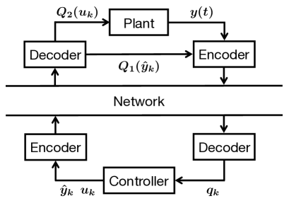
Figure 2: Closed-loop system with input and output quantization.

Remark 8

Instead of (26), we can use different controllers such as

$$\Sigma_{C}^{\prime\prime}:\begin{cases}\begin{aligned} \hat{x}_{k+1}&=A_{d}\hat{x}_{k}+B_{d}Q_{2}(u_{k})+L(q_{k}-Q_{1}(\hat{y}_{k}))\\ \hat{y}_{k}&=C\hat{x}_{k}\\ u_{k}&=-K\hat{x}_{k}.\end{aligned}\end{cases}$$

The major reason to use (26) is that if $\hat{x}_{0}=0$, then we have

$$\hat{x}_{k}=\sum_{\ell=0}^{k-1}(A_{d}-B_{d}K)^{k-\ell}(q_{\ell}-Q_{1}(y_{\ell}))$$ (27)

and hence $\hat{y}_{k}$ and $u_{k}$ can be described by $q_{\ell}-Q_{1}(y_{\ell})$, which makes encoding methods simple.

3.2 Output Encoding

Suppose that we obtain an error bound $E_{k}$ such that $|y_{k}-Q_{1}(\hat{y}_{k})|\leq E_{k}$. A bound sequence $\{E_{k}\}$ satisfying this condition is obtained in Section 3.4. Instead of (4), the encoder computes quantized measurements by dividing the hypercube

$$\left\{y\in\mathbb{R}^{\sf p}:~{}|y-Q_{1}(\hat{y}_{k})|_{\infty}\leq E_{k}\right\}$$ (28)

into $N^{\sf p}$ equal boxes. The difference between (4) and (28) is the quantization center. In (4), the encoder has the state estimate $\hat{x}_{k}$, and hence the quantization center can be $\hat{y}_{k}$. On the other hand, the encoder here employs the quantized output estimate $Q_{1}(\hat{y}_{k})$ reported by the controller as the quantization center. The rest of the output encoding is the same as in Subsection 3.2.

3.3 Estimate and Input Encoding

The controller sends the control input $u_{k}$ and the output estimate $\hat{y}_{k}$ to the plant side. Suppose that we have bounds $E_{1,k}$ and $E_{2,k}$ such that $|\hat{y}_{k}|\leq E_{1,k}$ and $|u_{k}|\leq E_{2,k}$. Such a bound sequence $\{(E_{1,k},E_{2,k})\}$ is obtained in Section 3.4. The bounds and levels of the quantization of $\hat{y},u$ are given by $(E_{1,k},N_{1})$ and $(E_{2,k},N_{2})$. Namely, the controller computes the quantized output estimate and the quantized input by dividing the hypercubes

$$\left\{\hat{y}\in\mathbb{R}^{\sf p}:~{}|\hat{y}|_{\infty}\leq E_{1,k}\right\}$$

$$\left\{u\in\mathbb{R}^{\sf m}:~{}|u|_{\infty}\leq E_{2,k}\right\}$$

into $N_{1}^{\sf p}$ and $N_{2}^{\sf m}$ equal boxes and assigns a number in $\{1,\dots,N_{1}^{\sf p}\}$ and $\{1,\dots,N_{2}^{\sf m}\}$ to each divided box by a certain one-to-one mapping, respectively. The decoder in the plant side generates $Q_{1}(\hat{y}_{k})$ and $Q_{2}(u_{k})$ equal to the center of the boxes with number reported by the controller. Thus $Q_{1}(\hat{y}_{k})$ and $Q_{2}(u_{k})$ satisfy

$$|\hat{y}_{k}-Q_{1}(\hat{y}_{k})|\leq\frac{E_{1,k}}{N_{1}},\quad|u_{k}-Q_{2}(u_{k})|\leq\frac{E_{2,k}}{N_{2}}.$$ (29)

Since $\hat{x}_{0}=0$, we can set the initial values

$$E_{1,0}:=0,\quad E_{2,0}:=0.$$

The encoding strategy (28) of the output $y_{k}$ uses the quantized output estimate $Q_{1}(\hat{y}_{k})$ as the quantization center, whereas the quantization centers for the output estimate $\hat{y}_{k}$ and the input $u_{k}$ are the origin, which allows the plant side to have less computational resources.

Remark 9

Although the encoder does not have to estimate output measurements, the bounds $E_{k}$, $E_{1,k}$, and $E_{2,k}$ should be computed in the plant side. However, these bounds can be calculated by simple difference equations (31) as shown in the next subsection. If components in the plant side do not have computational resources enough to implement those difference equations, the controller can send sufficiently accurate values of the bounds even in the presence of quantization, because the dimension of each bound is one.

3.4 Computation of Bound Sequence $\{(E_{k},E_{1,k},E_{2,k})\}$

The following theorem is an extension of Theorem 4.

Theorem 10

Let Assumptions 1 and 2 hold, and define $R$ and $\bar{R}$ as in (6). Let the observer gain $L$ and the feedback gain $K$ satisfy $r(R)<1$, $r(\bar{R})<1$ and

$$\|CR^{\ell}\|\leq M_{0}\rho^{\ell},\quad\|C\bar{R}^{\ell}L\|\leq M_{1}\bar{\rho}^{\ell},\quad\|K\bar{R}^{\ell}L\|\leq M_{2}\bar{\rho}^{\ell}$$

$$\|CR^{\ell}B_{d}\|\leq M_{3}\rho^{\ell},\quad\|CR^{\ell}L\|\leq M_{4}\rho^{\ell}$$

hold for some $M_{0},M_{1},M_{2},M_{3},M_{4}>0$ and $\bar{\rho}\leq\rho<1$. Define constants $\alpha_{0}$ and $\alpha_{1}$ by

$$M :=(N-1)\cdot\left(\frac{M_{1}M_{4}}{N_{1}}+\frac{M_{2}M_{3}}{N_{2}}\right)$$

$$\beta_{0} :=\rho+\frac{N_{1}M_{4}+(N-1)M_{1}}{NN_{1}}$$

$$\beta_{1} :=\frac{M}{N}$$

$$\alpha_{0} :=\rho+\beta_{0}$$

$$\alpha_{1} :=\beta_{1}-\rho\beta_{0}.$$

If we pick $N,N_{1},N_{2}\geq 2$ so that

$$F:=\begin{bmatrix}\alpha_{0}&\alpha_{1}\\ 1&0\end{bmatrix}$$ (30)

satisfies $r(F)<1$, then the proposed encoding method with a bound sequence $\{(E_{k},E_{1,k},E_{2,k})\}$ defined by

$$E_{k+1}:=\begin{cases}M_{0}E_{st}\rho+\left(M_{4}+\frac{(N-1)M_{1}}{N_{1}}\right)\frac{E_{0}}{N}&k=0\\ \beta_{0}E_{k}+\beta_{1}E_{k-1}&k=1\\ \alpha_{0}E_{k}+\alpha_{1}E_{k-1}&k\geq 2\end{cases}$$

$$E_{1,k+1}:=\bar{\rho}E_{1,k}+\frac{(N-1)M_{1}}{N}E_{k}\hskip 67.5ptk\geq 0$$

$$E_{2,k+1}:=\bar{\rho}E_{2,k}+\frac{(N-1)M_{2}}{N}E_{k}\hskip 67.5ptk\geq 0.$$ (31)

achieves the exponential convergence of the state $x$ and the estimate $\hat{x}$.

The error $e_{k+1}=x_{k+1}-\hat{x}_{k+1}$ satisfies

$$e_{k+1} =R^{k+1}e_{0}+\sum_{\ell=0}^{k}R^{\ell}\big{(}L(y_{k-\ell}-q_{k-\ell})$$

$$\qquad\qquad\qquad-L(\hat{y}_{k-\ell}-Q_{1}(\hat{y}_{k-\ell}))$$

$$\qquad\qquad\qquad-B_{d}(u_{k-\ell}-Q_{2}(u_{k-\ell}))\big{)}.$$ (32)

On the other hand, since $\hat{x}_{0}=0$, it follows that

$$\hat{x}_{k+1}=\sum_{\ell=0}^{k}\bar{R}^{\ell}L(q_{k-\ell}-Q_{1}(\hat{y}_{k-\ell})).$$

Since $Q_{1}(\hat{y}_{k})$ is the quantization center and $q_{k}$ is the quantization value, we have

$$|q_{k}-Q_{1}(\hat{y}_{k})|\leq(N-1)\mu_{k}$$

for all $k\geq 1$. Hence $\hat{y}_{k}$ and $u_{k}$ satisfy

$$\begin{array}[]{c}|\hat{y}_{k}|\leq\frac{(N-1)M_{1}}{N}\sum_{\ell=0}^{k-1}\bar{\rho}^{\ell}E_{k-\ell-1}=:E_{1,k}\\[15.0pt] |u_{k}|\leq\frac{(N-1)M_{2}}{N}\sum_{\ell=0}^{k-1}\bar{\rho}^{\ell}E_{k-\ell-1}=:E_{2,k}\end{array}$$ (33)

for all $k\geq 1$. Since $E_{i,k}$ in (33) satisfies

$$E_{i,k+1}-\bar{\rho}E_{i,k}=\frac{(N-1)M_{i}}{N}E_{k},\qquad i=1,2,$$

we obtain the difference equations (31) for $E_{1,k}$ and $E_{2,k}$.

On the other hand, for every $k\geq 0$, define $E_{k+1}$ by

$$E_{k+1}:=M_{0}E_{st}\rho^{k+1} +\sum_{\ell=0}^{k}\left(M_{4}+\frac{(N-1)M_{1}}{N_{1}}\right)\rho^{\ell}\mu_{k-\ell}$$

$$+M\sum_{\ell=0}^{k-1}\sum_{i=0}^{k-\ell-1}\rho^{\ell+i}\mu_{k-\ell-i-1}.$$ (34)

Combining (29), (32), and (33), we have that for all $k\geq 0$,

$$|y_{k+1}-Q_{1}(\hat{y}_{k+1})| \leq|y_{k+1}-\hat{y}_{k+1}|+|\hat{y}_{k+1}-Q_{1}(\hat{y}_{k+1})|$$

$$\leq E_{k+1}.$$

Next we obtain the difference equation in (31) from (34). Since

$$\sum_{\ell=0}^{k-1}\sum_{i=0}^{k-\ell-1}\rho^{\ell+i}\mu_{k-\ell-i-1}=\sum_{\ell=0}^{k-1}\sum_{j=\ell}^{k-1}\rho^{j}\mu_{k-j-1},$$

it follows that for every $k\geq 1$, $E_{k+1}$ in (34) satisfies

$$E_{k+1} =\beta_{0}E_{k}+\beta_{1}\sum_{\ell=0}^{k-1}\rho^{\ell}E_{k-\ell-1}.$$

We therefore have

$$E_{k+1}-\rho E_{k}=\beta_{0}E_{k}+(\beta_{1}-\beta_{0}\rho)E_{k-1}$$

for every $k\geq 2$. Thus, we obtain the difference equation (31) for $E_{k}$.

If we define a vector ${\bm{\mu}}_{k}$ by

$${\bm{\mu}}_{k}:=\begin{bmatrix}\mu_{k}\\ \mu_{k-1}\end{bmatrix}$$

and a matrix $F$ as in (30), then we have the dynamics of ${\bm{\mu}}_{k}$, (23). Hence $\mu_{k}$ exponentially decreases to zero if and only if $F$ is Schur stable. Since the quantization errors of the input and the estimate also exponentially decrease from (31), the rest of the proof is the same as that of Theorem 4, and we therefore omit it. $\blacksquare$

Remark 11

Although we here generate $Q_{1}(\hat{y}_{k})$ and $Q_{2}(u_{k})$ separately, one can quantize $\hat{y}_{k}$ and $u_{k}$ simultaneously. This simultaneous quantization reduces the computational cost of the controller, but the data-rate condition for stabilization becomes conservative. Therefore, we do not proceed along this line.

Remark 12

There always exist quantization levels $N$, $N_{1}$, and $N_{2}$ such that the matrix $F$ in (30) satisfies $r(F)<1$. In fact, as $N$, $N_{1}$, and $N_{2}$ increase to infinity, we have $\alpha_{0}\to\rho$ and $\alpha_{1}\to\rho^{2}$, and hence the eigenvalues of $F$ tend to $\rho<1$.

4 Numerical Examples

4.1 Comparison of Data-Rate Conditions

First we consider the quantization of only the plant output and compare the data-rate conditions of three types of observers: the steady-state Kalman filter (7) with process noise covariance $10^{-3}$ and measurement noise covariance $10^{-5}\text{diag}(1,1)$, the deadbeat observer (21), and the pseudo-inverse observer (24). In addition to the output feedback case, we also investigate the state encoding case (25). In Table 1, we show the comparison of the minimum quantization level for exponential convergence, which are $N^{\sf p}$ in the output feedback case and $N^{\sf n}$ in the state feedback case. Note that steady-state Kalman filter and the deadbeat observers are represented by a linear time-invariant state equation but pseudo-inverse observers does not.

The first example is an inverted pendulum whose dynamics is given by (1) with

$$A:=\begin{bmatrix}0&1&0&0\\ 0&-20.06&53.26&-1.096\\ 0&0&0&1\\ 0&-20.01&98.41&-2.025\end{bmatrix},\quad B:=\begin{bmatrix}0\\ 35.28\\ 0\\ 35.18\end{bmatrix}$$ (35)

$$C:=\begin{bmatrix}1&0&1&0\end{bmatrix}.$$

The state $[x_{1}~{}~{}x_{2}~{}~{}x_{3}~{}~{}x_{4}]=:x$ are the arm angle, the arm angular velocity, the pendulum angle, and the pendulum angular velocity. The input $u$ is the motor voltage. Additionally, we borrow a 2-mass motor drive with one output and three states from Ji and Sul (1995), a pneumatic cylinder with one output and three states from Kimura et al. (1996), and a batch reactor with two output and four states from Rosenbrock (1974).

In Table 1, we see that the Kalman filter requires less data-rate than the deadbeat observer and the pseudo-inverse observer for the 2-mass motor drive and the pneumatic cylinder. This is because the motor drive and the cylinder have their unstable poles only on the imaginary axis. Hence the observer gain of the Kalman filter is small, which decreases $M$ in (7). Although deadbeat observers and pseudo-inverse observers have the same property: finite-time state reconstruction in the idealized situation without quantization, the data-rate condition (24) by pseudo-inverse observers is better than that (21) by deadbeat observers. This is because pseudo-inverse observers employ output measurements directly for state reconstruction, whereas deadbeat observers summarize output information by their states. Moreover, compared with the state feedback case (25), the output feedback case requires small data sizes in most numerical examples because the state dimension ${\sf n}$ and the output dimension ${\sf p}$ satisfy ${\sf n}>{\sf p}$.

Table 1: Minimum quantization levels for exponential convergence.

	Kalman filter (7)	Deadbeat observer (21)	Pseudo-inverse observer (24)	State encoding (25)
Inverted pendulum ($h=0.03$)	$5^{2}=25$	$4^{2}=16$	$4^{2}=16$	$4^{4}=256$
2-mass motor drive ($h=10^{-3}$)	$5^{1}=5$	$7^{1}=7$	$3^{1}=3$	$3^{3}=27$
Pneumatic cylinder ($h=10^{-3}$)	$2^{1}=2$	$7^{1}=7$	$3^{1}=3$	$2^{3}=8$
Batch reactor ($h=0.1$)	$23^{2}=529$	$4^{2}=16$	$4^{2}=16$	$3^{4}=81$

4.2 Time response of Inverted Pendulum

Consider again the inverted pendulum in the previous subsection. Next we compute the time response of the inverted pendulum described by (35) with considering quantization of the plant input and output. The controller is assumed to send to the encoder the quantized value of the output estimate for quantization centers. Let the sampling period be $h=0.03$ sec. We set the feedback gain $K$ to be the quadratic regulator whose weighting matrices of the state and the input are $\text{diag}(100,0,300,0)$ and $1$, respectively. The observer gain $L$ is the Kalman filter whose covariances of the process noise and measurement noise are $10^{-3}$ and $10^{-5}\text{diag}(1,1)$, respectively.

From Theorem 10, the state $x$ exponentially converges to the origin under the proposed encoding strategy with $(N,N_{1},N_{2})=(151,301,1601)$ for which $F$ in (30) satisfies $r(F)=0.8845$.

Supposing that we obtain an initial state bound $E_{0}=0.15$, we compute a time response for the initial state $x(0)=[0~{}~{}0~{}~{}0.1~{}~{}0]^{\top}$. The plot of the arm angle $x_{1}$ and the pendulum angle $x_{3}$ is in Figs. 3 and 4. Fig. 5 illustrates the motor voltage $u$. From Figs. 3 and 4, we observe that the arm and pendulum angles decrease to zero in the presence of three types of quantization errors. Since the initial estimate $\hat{x}_{0}=0$, the quantization errors of the output estimate and the input are small at first. In fact, the output estimate bound $\{E_{1,k}\}$ and the input bound $\{E_{2,k}\}$ take the maximum value at about time $t=0.45$, and the effect of the quantization errors appears from time $t=0.5$ in Figs. 3, 4, and 5.

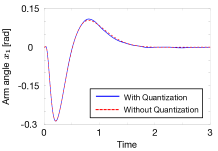
Figure 3: Arm angle $x_{1}$ with/without quantization.

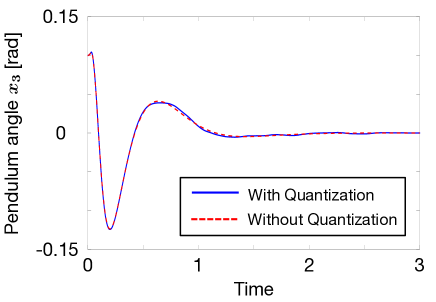
Figure 4: Pendulum angle $x_{3}$ with/without quantization.

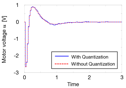
Figure 5: Motor voltage $u$ with/without quantization.

5 Conclusion

We studied quantized output feedback stabilization by Luenberger observers. Data-rate conditions for general Luenberger observers are characterized by the spectral radius of the system matrix of the error dynamics. On the other hand, a data-rate condition for deadbeat observers is determined by the behavior of the error dynamics for $\eta$ steps, where $\eta$ is the observability index of the plant. The proposed encoding method was also extended to case where both of the plant input and output are quantized and where the encoder does not have an estimator for generating quantization centers. Future work involves addressing more general systems such as nonlinear systems and switched systems.

References

• Brockett and Liberzon (2000) Brockett, R.W. and Liberzon, D. (2000). Quantized feedback stabilization of linear systems. IEEE Trans. Automat. Control, 45, 1279–1289.
• Ferrante et al. (2014) Ferrante, F., Gouaisbaut, F., and Tarbouriech, S. (2014). Observer-based control for linear systems with quantized output. In Proc. ECC’14.
• Ishii and Tsumura (2012) Ishii, H. and Tsumura, K. (2012). Data rate limitations in feedback control over network. IEICE Trans. Fundamentals, E95-A, 680–690.
• Ji and Sul (1995) Ji, J.K. and Sul, S.K. (1995). Kalman filter and LQ based speed controller for torsional vibration suppression in a 2-mass motor drive system. IEEE Trans. Ind. Electron., 42, 564–571.
• Kimura et al. (1996) Kimura, T., Fujioka, H., Tokai, K., and Takamori, T. (1996). Sampled-data $H_{\infty}$ control for a Pneumatic cylinder system. In Proc. IEEE 35th CDC.
• Liberzon (2003a) Liberzon, D. (2003a). Hybrid feedback stabilization of systems with quantized signals. Automatica, 39, 1543–1554.
• Liberzon (2003b) Liberzon, D. (2003b). On stabilization of linear systems with limited information. IEEE Trans. Automat. Control, 48, 304–307.
• Liberzon (2003c) Liberzon, D. (2003c). Switching in Systems and Control. Boston: Birkhäuser.
• Liberzon (2006) Liberzon, D. (2006). Quantization, time delays, and nonlinear stabilization. IEEE Trans. Automat. Control, 51, 1190–1195.
• Liberzon (2014) Liberzon, D. (2014). Finite data-rate feedback stabilization of switched and hybrid linear systems. Automatica, 50, 409–420.
• Liberzon and Hespanha (2005) Liberzon, D. and Hespanha, J.P. (2005). Stabilization of nonlinear systems with limited information feedback. IEEE Trans. Automat. Control, 50, 910–915.
• Liberzon and Nešić (2007) Liberzon, D. and Nešić, D. (2007). Input-to-state stabilization of linear systems with quantized state measurement. IEEE Trans. Automat. Control, 52, 767–781.
• Matveev and Savkin (2009) Matveev, A.S. and Savkin, A.V. (2009). Estimation and Control over Communication Networks. Birkhäuser, Boston.
• Nair and Evans (2004) Nair, G.N. and Evans, R.J. (2004). Stabilizability of stochastic linear systems with finite feedback data rates. SIAM J. Control Optim., 43, 413–436.
• Nair et al. (2007) Nair, G.N., Fagnani, F., Zampieri, S., and Evans, R.J. (2007). Feedback control under data rate constraints: An overview. Proc. IEEE, 95, 108–137.
• Okano and Ishii (2014) Okano, K. and Ishii, H. (2014). Stabilization of uncertain systems with finite data rates and Markovian packet losses. IEEE Trans. Control Network Systems, 1, 298–307.
• O’Reilly (1983) O’Reilly, J. (1983). Observer for Linear Systems. New York: Academic.
• Rosenbrock (1974) Rosenbrock, H.H. (1974). Computer-Aided Control System Design. New York: Academic Press.