Vision-based Real-Time Aerial Object Localization and Tracking for UAV Sensing System

Abstract

The paper focuses on the problem of vision-based obstacle detection and tracking for unmanned aerial vehicle navigation. A real-time object localization and tracking strategy from monocular image sequences is developed by effectively integrating the object detection and tracking into a dynamic Kalman model. At the detection stage, the object of interest is automatically detected and localized from a saliency map computed via the image background connectivity cue at each frame; at the tracking stage, a Kalman filter is employed to provide a coarse prediction of the object state, which is further refined via a local detector incorporating the saliency map and the temporal information between two consecutive frames. Compared to existing methods, the proposed approach does not require any manual initialization for tracking, runs much faster than the state-of-the-art trackers of its kind, and achieves competitive tracking performance on a large number of image sequences. Extensive experiments demonstrate the effectiveness and superior performance of the proposed approach.

I Introduction

In the last two decades, we have seen rapid growth in the applications of unmanned aerial vehicles (UAV). In the military, UAVs have been demonstrated to be an effective mobile platform in future combat scenarios. In civil applications, numerous UAV platforms have mushroomed and been applied to surveillance, disaster monitoring and rescue [9], package delivering [1], and aerial photography [22]. A number of companies are developing their own UAV systems, such as Amazon Prime Air [1], Google’s Project Wing [11], and DHL’s Parcelcopter [8]. In order to increase the flight safety, the UAV must be able to adequately sense and avoid other aircraft or intruders during its flight.

The ability of sense and avoid (SAA) enables UAVs to detect the potential collision threat and make necessary avoidance maneuvers. This technique has attracted lots of attention in recent years. Among all available approaches, vision-based SAA system [22, 25] is becoming more and more attractive since cameras are light-weighted and low-cost, and most importantly, they can provide richer information than other sensors. A successful SAA system should have the capability to automatically detect and track the obstacles. The study of these problems, as a central theme in computer vision, has been active for the past decades and achieved great progress.

Salient object detection in computer vision is interpreted as a process of computing a saliency map in a scene that highlights the visual distinct regions and suppresses the background. Most salient object detection methods rely on the assumption about the properties of objects and background. The most widely used assumption is contrast prior [5, 14, 15], which assumes that the appearance contrasts between the objects and backgrounds are very high. Several recent approaches exploit image background connectivity prior [45, 40], which assumes that background regions are usually connected to the image boundary. However, those methods lack of the capability to utilize the contextual information between consecutive frames in the image sequence.

On the other hand, given the position of the object of interest at the first frame, the goal of visual tracking is to estimate the trajectory of the object in every frame of an image sequence. The tracking-by-detection methods have become increasingly popular for real-time applications [42] in visual tracking. The correlation filter-based trackers attract more attention in recent years due to its high speed performance [4]. However, those conventional tracking methods [42, 41, 7, 20, 6, 44, 12, 32, 30, 19, 43] require manual initialization with the ground truth at the first frame. Moreover, they are sensitive to the initialization variation caused by scales and position errors, and would return useless information once failed during tracking [36].

Combining a detector with a tracker is a feasible solution for automatic initialization [2]. The detector, however, needs to be trained with large amount of training samples, while the prior information about the object of interest is usually not available in advance. In [24], Mahadevan et al. proposed a saliency-based discriminative tracker with automatic initialization, which builds the motion saliency map using optical flow. This technique, however, is computational intensive and not suitable for real-time applications. Some recent techniques on salient object detection and visual tracking [23, 13] have achieved superior performance by using deep learning. However, these methods need large amount of samples for training.

In [40], Zhang et al. proposed a fast salient object detection method based on minimum barrier distance transform. Since the saliency map effectively discovers the spatial information of the distinct objects in a scene, it enables us to improve the localization accuracy of the salient objects during tracking. In this paper, we propose a scale adaptive object tracking framework by integrating two complementary processes: salient object detection and visual tracking. A Kalman filter is employed to predict a coarse location of the object of interest. Then, a detector is used to refine the location of the object. The optimal state of the object in each frame is estimated relying on the recursive process of prediction, refining, and correction.

The proposed approach has been compared with the state-of-the-art detector and trackers on a sequence with challenging situations, including scale variation, rotation, illumination change, and out-of-view and re-apperance. As shown in Fig. 1, for object detection, the single view saliency detection algorithm (MB+) [40] is not able to provide high quality saliency maps for the image sequence because it does not manage to use the contextual information between consecutive frames; and from the tracking perspective, the existing trackers are not capable to handle out-of-view and re-appearance challenges.

In summary, our contributions are threefold: 1) The proposed algorithm integrates a saliency map into a dynamic model and adopts the target-specific saliency map as the observation for tracking; 2) we develop a tracker with automatic initialization for a UAV sensing system; and 3) the proposed technique achieves better performance than the state-of-the-art trackers from extensive experimental evaluations.

Our remaining part of this paper is organized as follows: Some related work is briefly reviewed in section II; in section III, the proposed approach is discussed thoroughly; in section IV, we demonstrate the quantitative and qualitative evaluation results, and some limitations; and finally, the paper is concluded in section V.

II Related Works

Salient object detection and visual tracking plays important roles in many computer vision based applications, such as traffic monitoring, surveillance, video understanding, face recognition, and human-computer interaction [37].

The task of salient object detection is to compute a saliency map and segment an accurate boundary of that object. For natural images, the assumptions on background and object have been shown to be effective for salient object detection [5, 45]. One of the most widely used assumptions is called contrast prior, which assumes high appearance difference between the object and background. Region-based salient object detection has become increasingly popular with the development of superpixel algorithm [3]. In addition to contrast prior and region-based methods, several recent approaches exploit boundary connectivity [40, 45]. Wei et al. [33] proposed a geodesic saliency detection method based on contrast, image boundary, and background priors. The salient object is extracted by finding the shortest path to the virtual background node. Zhu et al. [45] formulated the saliency detection as an optimization problem and solved it by a combination of superpixel and background measurement. Cheng et al. [5] computed the global contrast using the histogram and color statistics of input images. These state-of-the-art saliency detection methods achieve pixel-level resolution. Readers may refer to [3] for a comprehensive review on salient object detection.

The goal of visual tracking is to estimate the boundary and trajectory of the object in every frame of an image sequence. Designing an efficient and robust tracker is a critical issue in visual tracking, especially in challenging situations, such as illumination variation, in-plane rotation, out-of-plane rotation, scale variation, occlusion, background clutter and so on [36]. Over the past decades, various tracking algorithms have been proposed to cope with the challenges in visual tracking. According to the models adopted, these approaches can be generally classified into generative models [27, 31, 38, 39], and discriminative models [42, 24, 16]. Ross et al. [27] exploited an incremental subspace learning to visual tracking, which assumes that the obtained temporal targets reside in a low-dimensional subspace. Sui et al. [31] proposed a sparsity-induced subspace learning which selects effective features to construct the target subspace. Yin et al. [38] proposed a hierarchical tracking method based on the subspace representation and Kalman filter. Yu et al. [39] introduced a large-scale fiber tracking approach based on Kalman filter and group-wise thin-plate spline point matching.

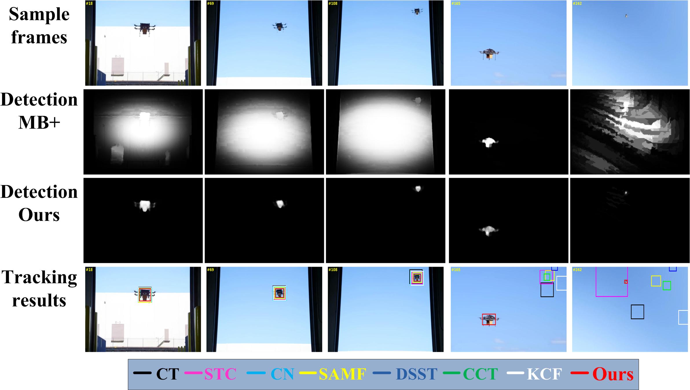
Figure 1: A comparison of the proposed approach with the state-of-the-art detector MB+ [40], and trackers CT [42], STC [41], CN [7], SAMF [20], DSST [6], CCT [44], KCF [12] on a sequence [1] with challenging situations, including scale variation, out-of-view and re-appearance. For detection, MB+ fails to provide a high quality saliency map. For tracking, the existing state-of-the-art trackers cannot handle the out-of-view and re-appearance challenges. Our method provides high quality of saliency map in detection, and accurate scale and position of the target in tracking.

The discriminative tracking-by-detection approaches have become increasingly popular in recent years. Zhang et al. [42] proposed a real-time tracker based on compressive sensing. Mahadevan et al. [24] proposed a saliency-based discriminative tracker, which learns the salient features based on Bayesian framework. Kalal et al. [16] introduced a long-term tracker which enables a re-initialization in case of tracking failures.

In particular, the correlation filter-based discriminative tracking methods have attracted much attention and achieved significant progress [4]. Henriques et al. [12] proposed a tracker using kernelized correlation filters (KCF). Zhu et al. [44] extended the KCF to a multi-scale kernelized tracker in order to deal with the scale variation. Zhang et al. [41] proposed a tracker via dense spatio-temporal context learning. Danelljan et al. [6] introduced a discriminative tracker using a scale pyramid representation. Li et al. [20] proposed to tackle the scale variation by integrating different low-level features. Danelljan et al. [7] designed a tracker by adaptive extension of color attributes. Readers can refer to [37, 28] and the references therein for details about visual tracking.

III The Proposed Approach

The proposed fast object localization and tracking (FOLT) algorithm is formulated within a robust Kalman filter framework [38, 35] to estimate the optimal state of the salient object from the saliency map in every frame of a given image sequence. Our tracking approach relies on a recursive process of prediction, object detection, and correction, as shown in Fig. 2. A linear dynamic (with constant velocity) model has been employed to represent the transition of the motion state of the salient object in a scene [35]. The tracker is initialized on the first frame using the saliency map computed on the entire image. The motion state is predicted on each frame according to the motion states of previously obtained object of interest. Under the constraint of natural scenes, the prediction is not far away from the ground truth [38], however, it only provides a coarse state estimation (“predicted bounding box” shown in Fig. 2) about the target location. We take this predicted coarse location as an initial region for further estimation during object tracking. The refined target is marked by a bounding box on that frame according to its motion state. Finally, the Kalman gain and a posteriori error covariance in the dynamic model are updated. The details about prediction, object localization and correction scheme are discussed in the following.

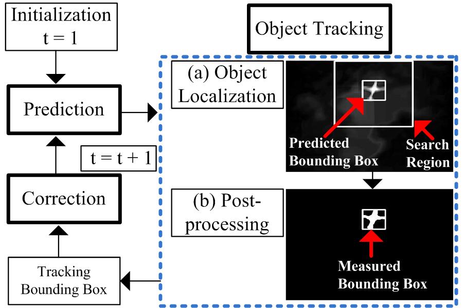
Figure 2: The flow-chart of the proposed fast object localization and tracking strategy.

III-A Dynamic model formulation

In the dynamic model, the object of interest is defined by a motion state variable $s=\{x,y,u,v,w,h\}$, where $(x,y)$ denotes the center coordinates, $(u,v)$ denotes its velocities, and $(w,h)$ denotes its width and height. The state at each frame $t+1$ is estimated using a linear stochastic difference equation $s(t+1)=Hs(t)+u(t)+w(t)$, where the prediction noise $w(t)\sim N(0,Q)$ is Gaussian distributed with covariance $Q$, $u(t)\in\mathcal{R}^{l}$ is a driving function with dimension $l$. The vector $s\in\mathcal{R}^{n}$ describes the motion states of the salient object. The orthogonal transition matrix $H\in n\times n$ evolves the state from the previous frame $t$ to the state at the current frame $t+1$. The vector $y(t)\in\mathcal{R}^{m}$ is denoted as an observation or measurement with dimension $m$ measured in frame $t$. In our notation, we will define $s_{t}\equiv s(t)$, and $y_{t}\equiv y(t)$. With the driving function removed from our model, the autoregressive model of the salient object in a frame is built based on the following linear stochastic model

$$s_{t+1}=Hs_{t}+w_{t},w_{t}\sim N(0,Q)\,,$$ (1)

$$y_{t}=Cs_{t}+v_{t},v_{t}\sim N(0,R)\,,$$ (2)

where the measurement matrix $C$ is $m\times m$, and the measurement noise $v_{t}\sim N(0,R)$ is Gaussian distributed with covariance $R$. The diagonal elements in the prediction noise covariance matrix $Q$ and measuremnt noise matrix $R$ represent the covariance of the size and position.

In the $t$-th frame, given the probability of $y_{t}$ and all the previously obtained states from the first to $(t-1)$-th frame, denoted as $s_{1:t-1}$, the optimal motion state of the target in the $t$-th frame, denoted as $s_{t}$, is predicted by maximizing the posterior probability $p(s_{t}|y_{t},s_{1:t-1})$. To simplify our model, we inherit the Markov assumption, which states that the current state is only dependent on the previous state. Therefore, the objective function becomes

$$\hat{s}_{t}=\arg\underset{s}{max}\quad p(s_{t}|y_{t},s_{t-1})\,.$$ (3)

Using Bayes formula, the posterior probability becomes:

$$p(s_{t}|y_{t},s_{t-1})=\frac{p(y_{t}|s_{t},s_{t-1})p(s_{t}|s_{t-1})}{p(y_{t})}\,,$$ (4)

where the denominator $p(y_{t})$ is a normalization constant, which indicates the prior distribution of the observation $y_{t}$. The observation $y_{t}$ is not dependent on the previous state $s_{t-1}$ in the presence of $s_{t}$, since $y_{t}$ is only generated by the state $s_{t}$. Thus equation (4) is reduced to:

$$p(s_{t}|y_{t},s_{t-1})=p(y_{t}|s_{t})p(s_{t}|s_{t-1})\,,$$ (5)

where the observation model $p(y_{t}|s_{t})$ measures the likelihood to be the target of the measurement $y_{t}$ with the motion state $s_{t}$. Finally, we formulate the objective function as

$$\hat{s}_{t}=\arg\underset{s}{max}\quad p(y_{t}|s_{t})p(s_{t}|s_{t-1})\,.$$ (6)

The state estimation can be converted to the standard Kalman filter framework [34] when we assumed that the state transition model and the observation model follow a Gaussian distribution.

III-B Object tracking

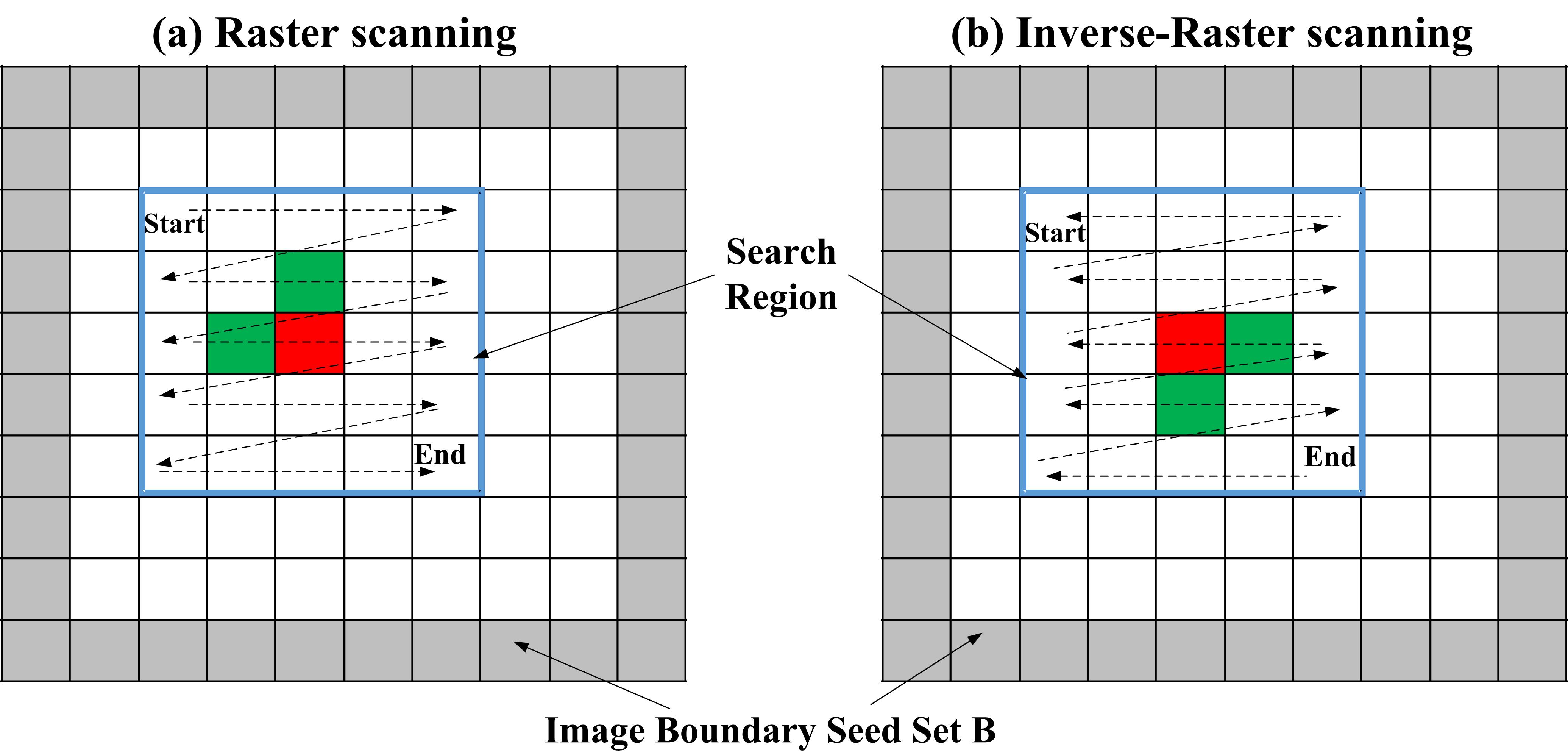
Figure 3: Illustration of updating the search region on a 4-adjacent graph using (a) Raster scanning, to update the intensity value at pixel $z$ (red box) using its two adjacent neighbors (green boxes) in search region from “Start” to “End” line by line, (b) Inverse-raster scanning, using the same updating strategy in opposite direction from ”End” to ”Start”.

The step of object tracking consists of two procedures: to implement object localization in the search region; and to infer the target state after conducting the post-processing on the saliency map.

III-B1 Object localization

A background prior, i.e., the image boundary connectivity cue [40], has been applied to locate the object in each frame. However, the proposed localization method has two obvious differences. First, by integrating with the contextual information, the proposed approach is capable to localize the salient object in both individual images and video sequences. Second, to leverage this cue, the saliency map, which represents the probability of a certain region in an image to be a salient object or background, is updated locally based on the coarse prediction (“predicted bounding box” shown in Fig. 3).

In this paper, we will denote $I_{t}$ as the image on the $t$-th frame. Firstly, on the frame $t$, under the constrain of natural image [35], it is reasonable to define a search region, where the salient object is guaranteed to exist, by expanding the predicted bounding box with certain percentage $\delta$. Next, the saliency map $D$ in the search region is updated by computing the minimum barrier distance [40, 29] with respect to a set of background seed set pixels $B$ (see illustration in Fig. 3). While the values for the pixels that are not in the search region are kept the same. Through those two steps, the position and scaling of the object is estimated on the frame $t$.

It is assumed under the image background connectivity cue that background regions are normally connected to the baground seed set $B$. In this paper, a path $p$ from pixel $1$ to pixel $n$ consists of a sequence of pixels, and is denoted as $p=\langle p(1),p(2),\cdots,p(n)\rangle$. In this sequence, each of the two consecutive pixels are neighbors. Each pixel in a 2-D single-channel image $I_{t}$ is denoted as a vertex. The neighboring pixels are connected by edges. In this work, we consider 4-adjacent neighbors as demonstrated in Fig. 3. For the image $I_{t}$, the cost function of computing the distance of a path from pixel $z$ to the background seed set $B$ is defined as finding the difference between the maximum and minimum intensity values in this path. The formula of the cost function is

$$F(p)=\max_{j=1}^{n}I_{t}(p(j))-\min_{j=1}^{n}I_{t}(p(j))\,,$$ (7)

where $I_{t}(\cdot)$ denotes the intensity value of a pixel in frame $t$. The saliency map $D(z)$ is obtained by minimizing the cost function $F(p)$,

$$D(z)=\underset{p\in\Theta_{B,z}}{min}F(p)\,,$$ (8)

where $p\in\Theta_{B,z}$ denotes the set, which includes all the possible paths from pixel $z$ to the background seed set $B$. This formulates the computation of the saliency map as a problem of finding the shortest path for each pixel in the image $I_{t}$. It can be solved by scanning each pixel using the Dijkstra-like algorithm. We denote $\langle m,z\rangle$ as the edge between two connected pixels $m$ and $z$, and $p(m)$ as the path asigned to pixel $m$, and $p_{m}(z)$ as the path connected pixel $m$ and pixel $z$ with edge $\langle m,z\rangle$. Therefore, the cost function of $p_{m}(z)$ is evaluated using

$$\begin{split}F(p_{m}(z))=&\max(U_{t}(m),I_{t}(z))-\\ &\min(L_{t}(m),I_{t}(z))\,,\end{split}$$ (9)

where $U_{t}(m)$ and $L_{t}(m)$ are matrices with the highest and lowest pixel values for the path $p(m)$, respectively. The initial values of $U$ and $L$ are identical with the image $I$. In the initial saliency map $D$, the region corresponding to the image boundary seed set $B$ is initialized with intensity of zeros, and the left pixels are initialized with intensity of infinity. The raster scanning pass and inverse-raster scanning pass are implemented alternately to update the saliency map $D$, as shown in Fig. 3. The number of passes is denoted as $N$, and in this paper we select $N=3$. In the raster scanning pass, each pixel in the search region is visited line by line. The intensity value at pixel $z$ is updated using its two neighbors (as illustrated in Fig. 3). The inverse-raster scanning applies the same updating but in an opposite order. The updating strategy of saliency map $D(z)$ is

$$D(z)\leftarrow\min\left\{\begin{array}[]{l}D(z)\\ F(p_{m}(z))\end{array}\right.\,.$$ (10)

III-B2 Post-processing

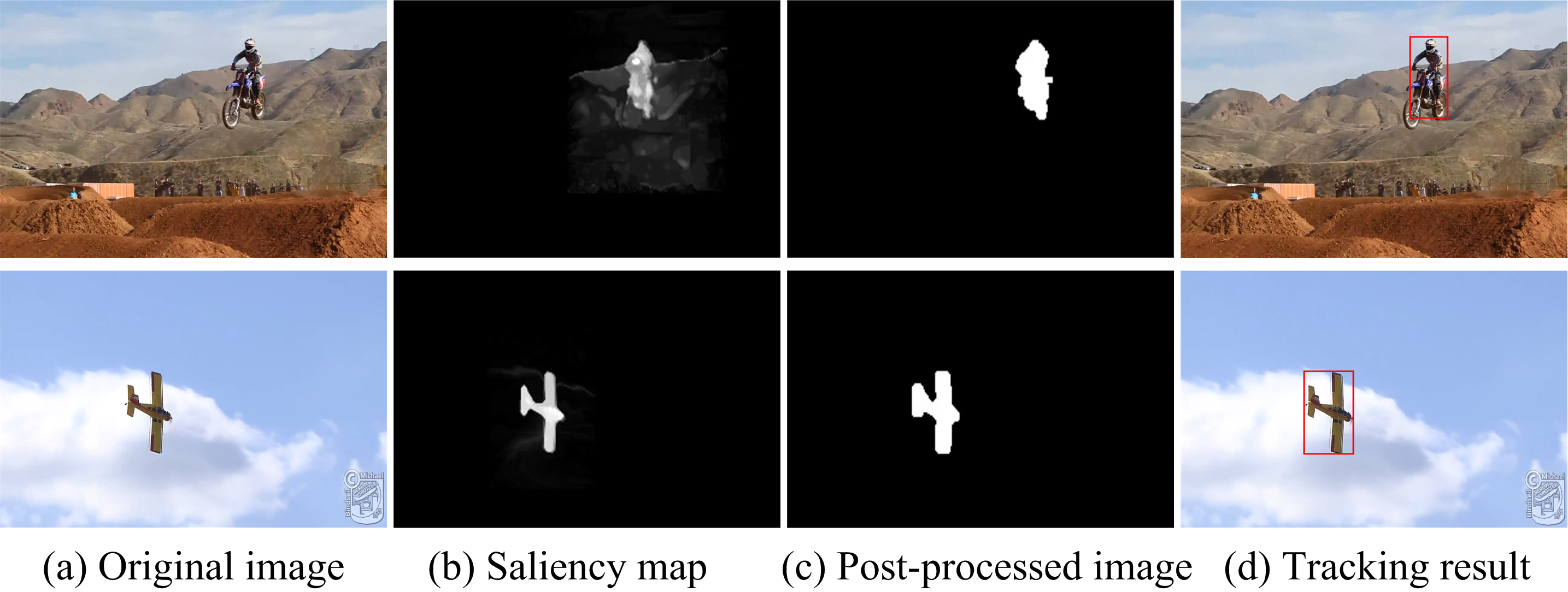
Figure 4: Illustration of the intermediate processes, including salient object detection, localization and post-processing in the proposed tracking approach. The two image sequences are motorcycle_011 (frist row) [18] and airplane_016 (second row) [18].

Two efficient post-processing operations have been implemented to improve the quality of the saliency map, and to further segment the salient object in every frame. A Threshold is applied to the saliency map, which transforms the saliency map to a binary image. Then, the tracking bounding box is extracted after dilation (see Fig. 2). Global threshold is not an efficient solution in the scenario where image has non-uniform illumination and lighting conditions. Hence, it is wise to employ adaptive threshold [10]. We denote $m_{ab}$ as the mean value of the set of pixels contained in a neighboring block, $\Gamma_{ab}$, centered at coordinates $(a,b)$ in an image. The size of the block $\Gamma_{ab}$ is $\alpha\times\alpha$. The following formula defines the local thresholds

$$T_{ab}=m_{ab}-\lambda\,,$$ (11)

where $\lambda$ is a nonnegative offset. The segmented image is computed as

$$f(a,b)=\left\{\begin{array}[]{ll}$1$,\quad\text{if $g(a,b)$}\geq T_{ab}\\ $0$,\quad\text{otherwise}\end{array}\right.\,,$$ (12)

where $g(a,b)$ is the input saliency map image. The equ. (12) is evaluated for all pixels in the image, and a threshold is calculated at each position $(a,b)$ using the pixels in the neighboring block of $\Gamma_{ab}$. The idea of dilation is applied to enhance the quality of the thresholded image $f(a,b)$. The dilation of $A$ by $S$, denoted by $A\oplus S$, is defined as

$$A\oplus S=\{q|\hat{(S)}_{q}\cap A\neq\varnothing\}\,,$$ (13)

where $S\in\mathcal{R}^{O\times M}$ is a structuring element. After dilation, the minimum bounding box of the extracted region gives the state estimation $\hat{s}_{t}$ of the target. Fig. 4 shows examples on two sequences (motorcycle_011 and airplane_016). The tracking bounding box is estimated by passing the original image through the processes of salient object detection and post-processing.

III-C Fast object localization tracking

Input: image $I_{t}$, saliency map $D$, number of pass $N$

Output: target state $\hat{s}_{t}$

1 Set $D$ to $\infty$ in search region and $B$

2 Keep the values in $D$ outside the search region

3 for each frame do

4       Prediction in Kalman filter

5       Object tracking:

6       for $i=1:N$ do

7             if mod$(i,2)=1$ then

8                  Raster Scanning using (10)

9             end if

10            else

11                   Inverse-Raster Scanning using (10)

12             end if

13            

14       end for

15      Observation: update measurement using (2)

16       Correction: update (14), (16)

17      

18 end for

Compute the entire $D$ every $10$ frames

Algorithm 1 Fast Object Localization Tracking

In this section, we denote $G_{t}^{-}$ and $G_{t}$ as a priori error covariance and a posteriori error covariance, respectively. In the correction stage of frame $t$, both of the posterior error covariance and Kalman gain are updated as follows.

1. Compute Kalman gain

   $$K_{t}=\frac{H^{T}}{G_{t}(HG_{t}^{-}H^{T}+R)}$$ (14)

2. Update estimate with measurement $y_{t}$

   $$\hat{s}_{t}=\hat{s}_{t}^{-}+K_{t}(y_{t}-C\hat{s}_{t}^{-})$$ (15)

3. Compute a posteriori error covariance

   $$G_{t}=(\mathcal{I}-K_{t}H)G_{t}^{-}$$ (16)

In summary, through the recursive prediction, object localization, and correction, the salient object in a image sequence is automatically detected and tracked. The details of the fast object localization tracking is illustrated in Alg. 1. The saliency map $D$ is updated on the entire image every $10$ frames as a trade-off between the accuracy and the speed.

IV Experimental Evaluations

TABLE I: Attributes used to characterize each image sequence from a tracking perspective. We denote scale variation as SV, illumination variation as IV, background interference as BGI, and in-plane rotation and out-of-plane rotation as IPR & OPR.

Image Sequence	Object of Interest	Tracking challenges
Aircraft [26]	Propeller plane	SV, IPR & OPR
airplane_001 [18]	Jet plane	SV, IPR & OPR
airplane_006 [18]	Jet plane	SV, IPR & OPR
airplane_011 [18]	Propeller plane	SV, IPR & OPR
airplane_016 [18]	Propeller plane	SV, IPR & OPR, BGI
big_2 [26]	Jet plane	SV, IPR & OPR, BGI
Plane_ce2 [21]	Jet plane	SV, IPR & OPR, BGI
Skyjumping_ce [21]	Person	SV, IV, IPR & OPR, BGI
motorcycle_006 [18]	Person and motorcycle	SV, IPR & OPR, BGI
surfing [17]	Person	SV, IPR & OPR, BGI
Surfer [36]	Person	SV, IPR & OPR, BGI
Skater [36]	Person	SV, IPR & OPR, BGI
Sylvester [36]	Doll	IV, IPR & OPR, BGI
ball [17]	ball	SV, BGI
Dog [36]	Dog	SV, OPR

The proposed approach is implemented in C++ with OpenCV 3.0.0 on a PC with an Intel Xeon W3250 2.67 GHz CPU and 8 GB RAM. The dataset and source code of the proposed approach will be available on the author’s homepage. The proposed tracker is evaluated on 15 popular image sequences collected from [18, 21, 17, 36]. There are a total of over 6700 frames in the dataset. The highest and lowest frame sizes are $1280\times 720$ and $320\times 240$, respectively. The dataset, from tracking perspective of view, includes different scenarios with challenging situations, such as scale variation, occlusions, in-plane and out-of-plane rotations, illumination, and background interference, as shown in Table. I. The image sequences without sky-region scenarios, i.e. Skyjumping_ce, motorcycle_006, surfing, Surfer, Skater, Sylvester, ball and Dog have been selected to test the robustness and generality of the proposed approach within different scenarios. In each frame of these video sequences, we labeled the target manually in a bounding box, which is used as the ground truth in the quantitative evaluations.

In our implementation, input images are first resized so that the maximum dimension is 300 pixels. The transition state matrix $H\in\mathcal{R}^{6\times 6}$ and measurement matrix $C\in\mathcal{R}^{4\times 6}$ are fixed during the experiment. The diagonal values corresponding to the position (i.e., $(x,y)$) and scale (i.e., $(w,h)$) covariance in prediction noise covariance matrix $Q$ and measurement covariance matrix $R$ are set to $0.01$ and $0.1$, respectively. Some other parameters for all image sequences are as follows. The percentage value $\delta=0.25$, the size of block $\Gamma_{ab}$ is $5\times 5$, the offset $\lambda=7$, and the structuring element is $S\in\mathcal{R}^{5\times 3}$.

We compared the proposed approach with seven state-of-the-art trackers. The seven competing trackers are manually initialized at the first frame using the ground truth of the target object. Once initialized, the trackers automatically track the target object in the remaining frames. However, the proposed tracker automatically runs to track the target object from the first frame to the end frame. Three experiments are designed to evaluate trackers as discussed in [36]: one pass evaluation (OPE), temporal robustness evaluation (TRE), and spatial robustness evaluation. For TRE, we randomly select the starting frame and run a tracker to the end of the sequence. Spatial robustness evaluation initializes the bounding box in the first frame by shifting or scaling. As discussed in Section III, the proposed method manages to automatically initialize the tracker and is not sensitive to spatial fluctuation. Therefore, we applied one pass evaluation and temporal robustness evaluation in this section using the same temporal randomization as in [36], and readers may refer to [36] for more details.

TABLE II: Quantitative evaluations of the proposed and the seven competing trackers on the 15 sequences. The best and second best results are highlighted in bold-face and underline fonts, respectively.

	Ours	CT	STC	CN	SAMF	DSST	CCT	KCF
		[42]	[41]	[7]	[20]	[6]	[44]	[12]
Precision of TRE	0.79	0.51	0.59	0.64	0.65	0.65	0.66	0.60
Success rate of TRE	0.61	0.45	0.46	0.54	0.58	0.56	0.57	0.52
Precision of OPE	0.83	0.44	0.48	0.44	0.59	0.48	0.66	0.48
Success rate of OPE	0.66	0.34	0.41	0.42	0.52	0.44	0.53	0.38
CLE (in pixel)	14.5	74.4	38.0	55.0	40.8	55.7	23.2	45.6
Average speed (in fps)	141.3	12.0	73.6	87.1	12.9	20.8	21.3	144.8

IV-A Speed performance

For salient object detection, the most up-to-date fast detector MB+ [40] attains a speed of 49 frames-per-second (fps). In contrast, the proposed method achieves a speed of 149 fps, three times faster than MB+, and the detection performance is better than MB+. For object tracking, the average speed comparison of the proposed and the seven state-of-the-art competing trackers is tabulated in Table II. The average speed of our tracker is 141 fps, which is at the same level as the fastest tracker KCF [12], however, KCF adopts a fixed tracking box, which could not reflect the scale changes of the target object during tracking. On average, our method is more than ten times faster than CT [42] and SAMF [20], five times faster than DSST [6] and CCT [44] and about two times faster than STC [41] and CN [7].

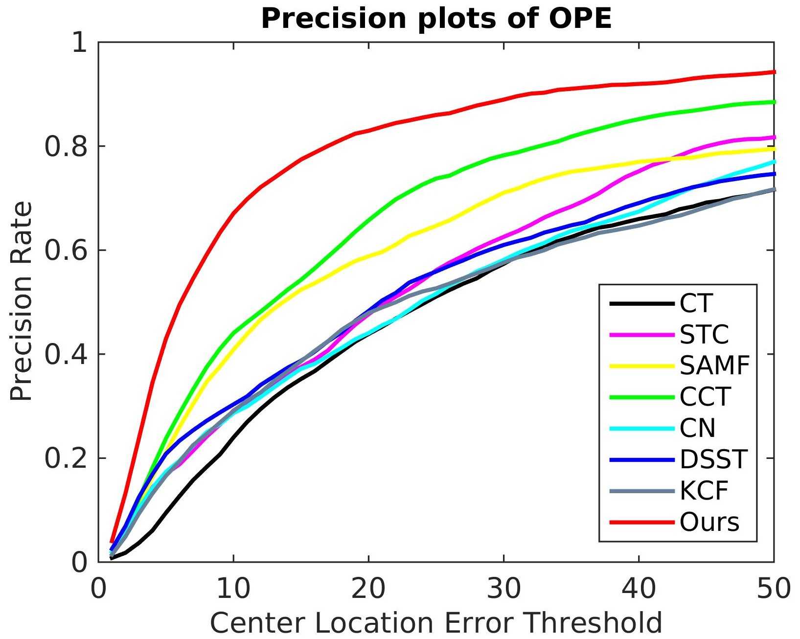
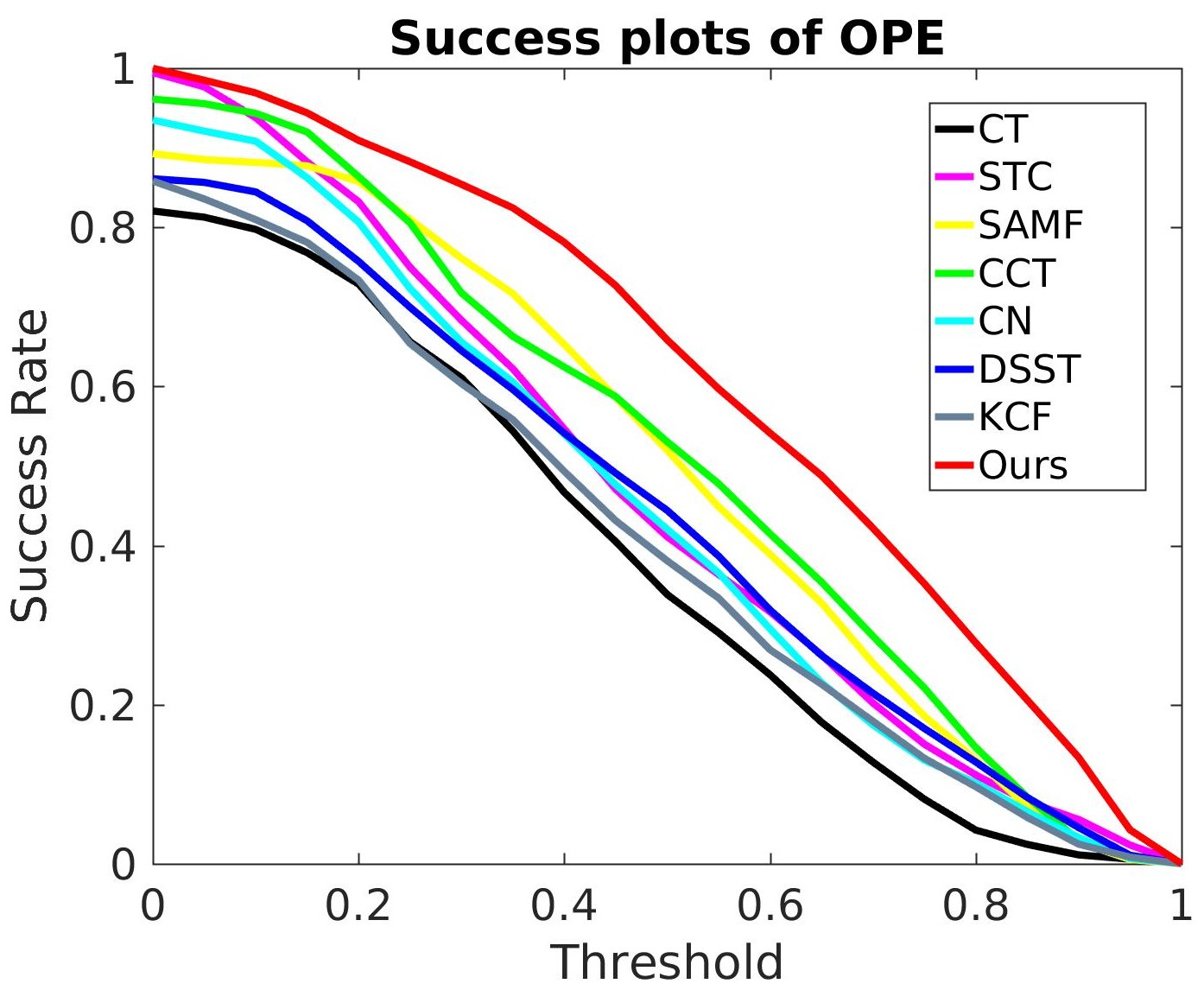
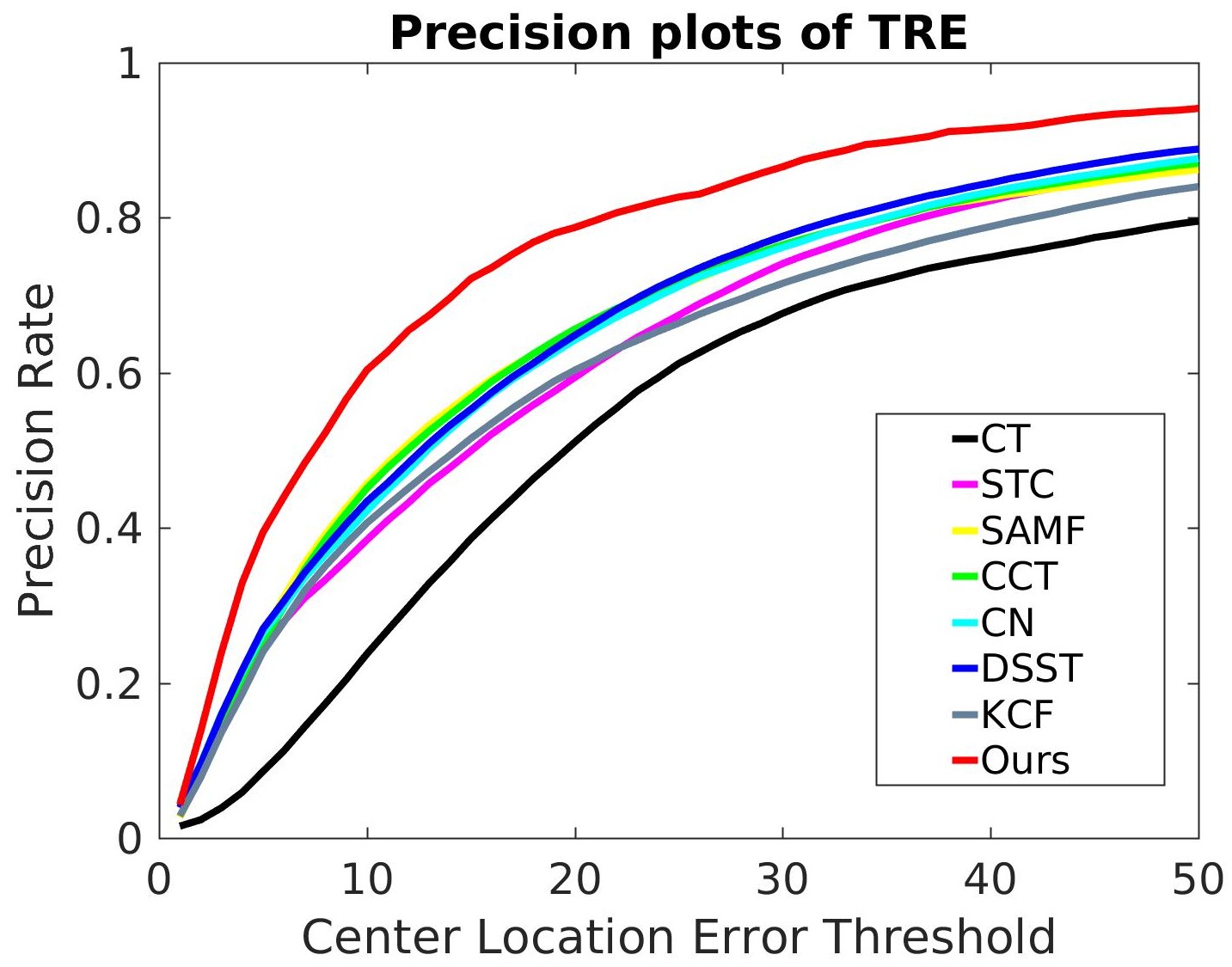
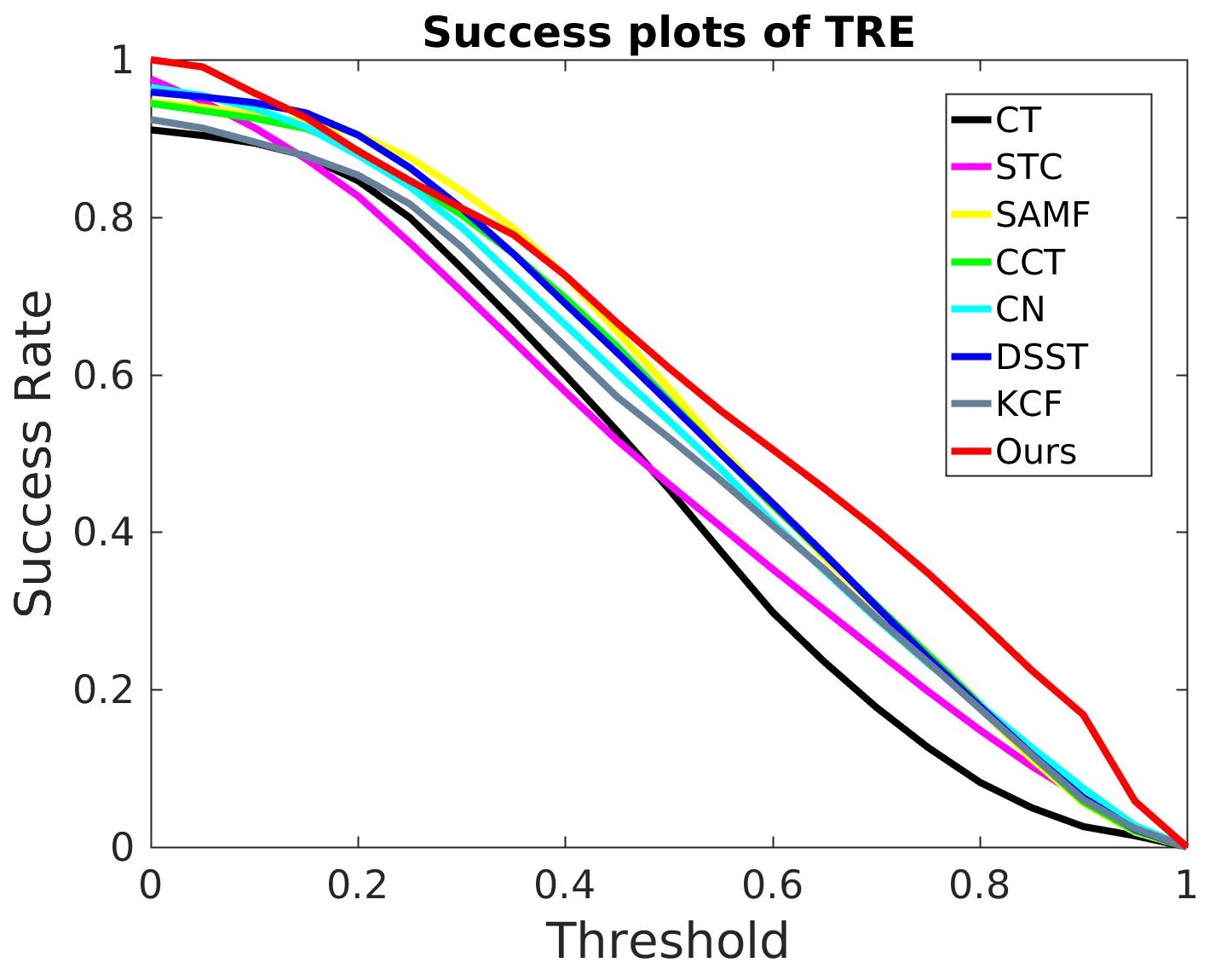
Figure 5: Average Precision and success rate plots over the 15 sequences in (top) one pass evaluation (OPE) and (bottom) temporal robustness evaluation (TRE). (best viewed in color)

IV-B Comparison with the state-of-the-art trackers

The performance of our approach is quantitatively evaluated following the metrics used in [36]. We present the results using precision, centre location error (CLE), and success rate (SR). The CLE is defined as the Euclidean distance between the centers of the tracking and the ground-truth bounding boxes. The precision is computed from the percentage of frames where the CLEs are smaller than a threshold. Following [36], the threshold value is set at 20 pixels for the precision in our evaluations. A tracking result in a frame is considered successful if $\frac{a_{t}\bigcap a_{g}}{a_{t}\bigcup a_{g}}>\theta$ for a threshold $\theta\in\left[0,1\right]$, where $a_{t}$ and $a_{g}$ denote the areas of the bounding boxes of the tracking and the ground truth, respectively. Thus, SR is defined as the percentage of frames where the overlap rates are greater than a threshold $\theta$. Normally, the threshold $\theta$ is set to 0.5. We evaluate the proposed method by comparing to the seven state-of-the-art trackers: CT, STC, CN, SAMF, DSST, CCT, and KCF.

The comparison results on the 15 sequences are shown in Table II. We present the results under one-pass evaluation and temporal robustness evaluation using the average precision, success rate, and CLE over all sequences. As shown in the table, the proposed method outperforms all seven competing trackers. It is evident that, in the one pass evaluations, the proposed tracker obtains the best performance in the CLE (14.5 pixels), and the precision (0.83), which are 8.7 pixels and $17\%$ superior to the second best tracker, the CCT tracker (23.2 pixels in CLE and 0.66 in precision). Meanwhile, in the success rate, the proposed tracker achieves the best result, which is a $13\%$ improvement against the second best tracker, the SAMF tracker. Please note that, for the seven competing trackers, the average performance in TRE is higher than that in OPE; while for the proposed tracker, the average precision and success rates in TRE are lower than those in OPE. One possible reason is that the proposed tracker tends to perform well in longer sequences, while the seven competing trackers work better in shorter sequences [36].

TABLE III: Precision on the 15 sequences of the proposed and the seven competing trackers. The best and the second best results are highlighted in bold-face and underline fonts, respectively.

	Ours	CT	STC	CN	SAMF	DSST	CCT	KCF
Aircraft	0.95	0.28	0.48	0.16	0.59	0.16	0.71	0.48
airplane_001	0.94	0.37	0.25	0.21	0.40	0.21	0.50	0.02
airplane_006	0.96	0.23	0.44	0.33	0.75	0.43	0.64	0.60
airplane_011	1.0	0.65	0.30	0.30	0.30	0.30	0.74	0.30
airplane_016	0.94	0.01	0.68	0.91	0.52	0.81	0.79	0.88
big_2	1.0	0.14	0.96	0.95	0.93	0.96	0.95	0.63
Skyjumping_ce	0.94	0.93	0.24	0.10	0.72	0.31	0.27	0.17
Plane_ce2	0.82	0.09	0.32	0.09	0.92	0.39	0.80	0.86
motorcycle_006	0.47	0.24	0.30	0.19	0.14	0.16	0.10	0.14
surfing	0.94	1.00	1.00	1.00	1.00	1.00	1.00	1.00
Skater	0.54	0.02	0.27	0.58	0.44	0.46	0.49	0.43
Surfer	0.59	0.35	0.48	0.51	0.43	0.34	0.46	0.22
Sylvester	0.87	0.62	0.59	0.93	0.85	0.84	0.84	0.84
ball	0.85	1.00	0.29	0.14	0.31	0.19	1.00	0.27
Dog	0.63	0.68	0.57	0.22	0.54	0.69	0.56	0.35
Average precision rate	0.83	0.44	0.48	0.44	0.59	0.48	0.66	0.48

We also report the comparison results in the one pass evaluation against the seven competing trackers on all 15 video sequences in Table III and Table IV, respectively. Our approach obtains the best or the second best performance of 14 in precision and 9 in success rate out of the 15 sequences. Fig. 5 plots the average precision and success plots in the one pass evaluation and temporal robustness evaluation over all 15 sequences. In the two evaluations, according to both the precision and the success rate, our approach significantly outperforms the seven competing trackers. In summary, the precision plot demonstrates that our approach is superior in robustness compared to its counterparts in the experiments; the success rate shows that our method estimates the scale changes of the target more accurately.

IV-C Qualitative evaluation

In this section, we present some qualitative comparisons of our approach with respect to the seven competing trackers. The proposed approach is generic and can be applied to track any object of interest, including non-rigid and articulated objects. In this section, we present qualitative results our tracker using eight representative image sequences to demonstrate the effectiveness using the dataset described in previous section. We assume the target object is in low resolution when more than one ground truth bounding box has less than 400 pixels. The eight image sequences are categorized into four groups based on their scenarios and tracking challenges, as shown in Table I.

The first group has clear sky as the background, including three image sequences, Aircraft, airplane_001 and airplane_006, which are shown from the first row to the third row in Fig. 6. All the three image sequences have scale variation and in-plane and out-of-plane rotations. The propeller plane in image sequence Aircraft are in high resolution. The jet planes in the other two image sequences are in low resolution, which increases the difficulity of tracking. Moreover, the background near the jet plane in the image sequence Airplane_006 has an appearance similar to the target. The competing trackers STC, SAMF, DSST, and CCT were proposed to deal with scale variation, but they failed in the three image sequences. The predicted bounding box is either too large or too small. The reason is that their scaling strategy depends on the hard-coded scaling ratio, which is not adaptive to rotation and scale variation of the target. In contrast, our tracker is based on a saliency map, which leads to an accurate localization of the salient object at each frame. Therefore, it is adaptive to scale and rotation variations, which gives more accurate estimation on both the scale and the position of the target object.

TABLE IV: Success rates on the 15 sequences of the proposed and the $7$ competing trackers. The best and the second best results are highlighted by bold-face and underline fonts, respectively.

	Ours	CT	STC	CN	SAMF	DSST	CCT	KCF
Aircraft	0.69	0.31	0.18	0.15	0.50	0.15	0.55	0.34
airplane_001	1.00	0.12	0.29	0.14	0.36	0.15	0.28	0.02
airplane_006	0.48	0.34	0.31	0.22	0.46	0.37	0.46	0.25
airplane_011	0.70	0.31	0.30	0.30	0.99	0.30	0.31	0.30
airplane_016	0.74	0.04	0.74	0.81	0.66	0.73	0.81	0.81
big_2	0.66	0.38	0.66	0.56	0.56	0.76	0.69	0.26
Plane_ce2	0.18	0.96	0.44	0.14	0.47	0.33	0.20	0.31
Skyjumping_ce	0.82	0.40	0.18	0.21	0.32	0.13	0.40	0.23
motorcycle_006	0.79	0.33	0.21	0.40	0.33	0.17	0.17	0.19
surfing	0.47	0.99	0.99	0.96	1.00	1.00	1.00	1.00
Skater	0.72	0.28	0.24	0.73	0.71	0.68	0.61	0.70
Surfer	0.68	0.31	0.08	0.51	0.69	0.65	0.70	0.25
Sylvester	0.73	0.71	0.71	0.71	0.97	0.85	0.92	0.97
ball	0.98	0.72	0.36	0.12	0.97	0.51	1.00	0.67
Dog	0.93	0.37	0.47	0.35	0.51	0.59	0.35	0.38
Average success rate	0.72	0.44	0.41	0.42	0.63	0.49	0.58	0.45

The second group with target object in high resolution includes three image sequences airplane_011, airplane_016, and big_2, which are illustrated in the fourth to the sixth rows in Fig. 6. The three image sequences have scale variation and in-plane and out-of-plane rotations challenges. Moreover, there still exists background interference caused by the clouds in the image sequences of airplane_016 and big_2. The background interference is more severe in the image sequence big_2 as the jet plane is at a lower altitude during its flight. Only the proposed tracker tracks the flying propeller plane accurately with giving the minimum bounding box of the target object in the image sequence of airplane_011. While most of the competing trackers are able to track the aircraft in the image sequences of airplane_016 and big_2, only the proposed approach has the capability to give the optimal tracking bounding box in the sky-region scenarios with clouds interference.

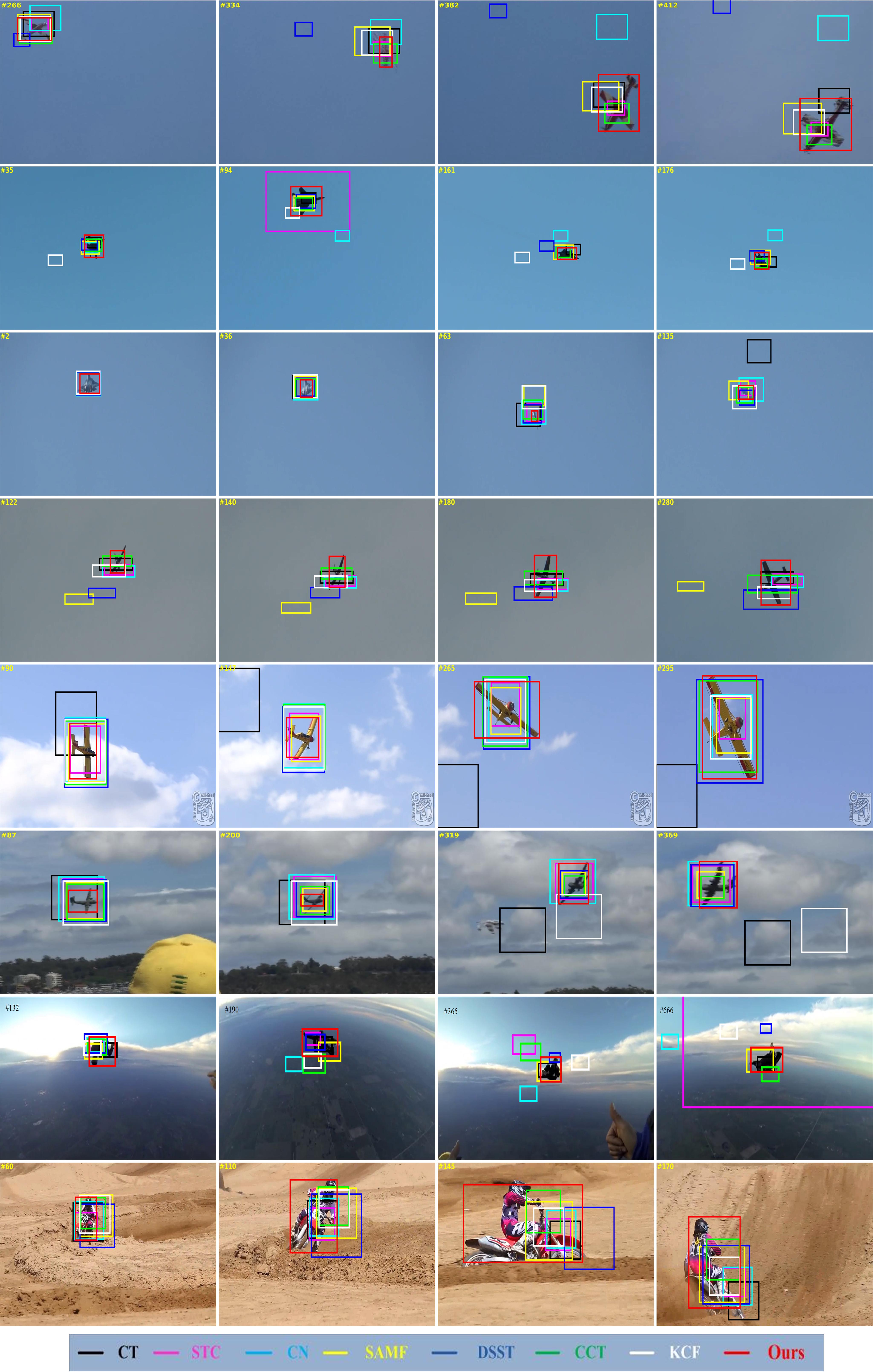
Figure 6: Tracking results in representative frames of the proposed and the $7$ competing trackers on eight sequences with different tracking challenges and scenarios. The first row: Aircraft [26]; the second row: airplane_001 [18]; the third row: airplane_006 [18]; the fourth row: airplane_011 [18]; the fifth row: airplane_016 [18]; the sixth row: big_2 [26]; the seventh row: Skyjumping_ce [21]; The eighth row: motorcycle_006 [18]. (best viewed in color)

The target object in the third group is a person doing sky jumping, as shown in the seventh row in Fig. 6. There exists small scale variation and large in-plane and out-of-plane rotations. Moreover, the clouds and terrain of the land in the background would interfere with the tracking performance. The competing trackers STC, SAMF, DSST, and CCT were capable to handle scale changes, but they failed in this image sequence. The competing trackers fail to handle the significant appearance changes of rotating motions and fast scale variations. In contrast, our tracker is robust to large and fast scale variations.

The proposed tracker can also be used to track the object of interest on the ground with large scale variation and out-of-plane rotation, as shown in the eighth row in Fig. 6. Since the cycler is driving the motorcycle with large rotation, the competing trackers can only track the head of the motorcycle, however, the proposed tracker is still able to give the minimum tracking bounding box of the object of interest, as shown from frame $\#110$ to frame $\#145$.

In summary, the proposed tracker has better performance than the seven competing trackers in handling large scale variation, in-plane and out-of-plane rotations with acute angle, and background cloud interference.

IV-D Limitation

Although the proposed tracking approach outperforms its competitors in most experiments, it has a key limitation in handling occlusion challenge. As shown in Fig. 7, the image sequence airplane_005, where the aircraft is partially (frame $\#86$) or severely (frame $\#96$) occluded by its ejected smoke and the cloud in the sky, which would cause a tracking failure. This failure can be automatically corrected by the tracker after a few frames, as shown in frame $\#102$. However, this limitation would deteriorate the performance of the tracker.

V Conclusion

In this paper, we have proposed an effective and efficient approach for real-time visual object localization and tracking, which can be applied to UAV navigation, such as obstacle sense and avoidance. Our method integrates a fast salient object detector within the Kalman filtering framework. Compared to the state-of-the-art trackers, our approach can not only initialize automatically, it also achieves the fastest speed and better performance than the competing trackers.

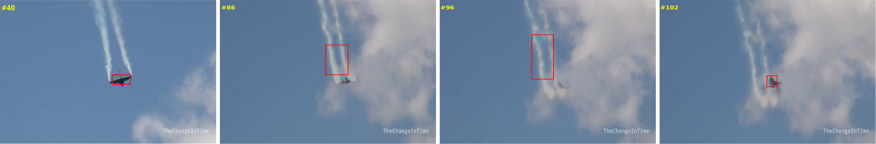
Figure 7: A failure case where the aircraft is partially or severely occluded in sequence airplane_005 [18] by the smoke and cloud.

Although the proposed tracker performs very well in most image sequences in our experiments, it cannot handle occluded scene very well. However, it has the capability to automatically re-localize and track the salient object of interest when it re-appears in the field of view again.

Yuanwei Wu received his Master’s degree from the Tufts University. He is currently a PhD candidate at the University of Kansas. His research interests are focused on broad applications in deep learning and computer vision, in particular object detection, localization and visual tracking.

Yao Sui received his Ph.D. degree in electronic engineering from Tsinghua University, Beijing, China, in 2015. He is currently a postdoctoral researcher in the Department of Electrical Engineering and Computer Science, University of Kansas, Lawrence, KS 66045, USA. His research interests include machine learning, computer vision, image processing and pattern recognition.

Guanghui Wang (M’10) received his PhD in computer vision from the University of Waterloo, Canada, in 2014. He is currently an assistant professor at the University of Kansas, USA. He is also with the Institute of Automation, Chinese Academy of Sciences, China, as an adjunct professor. From 2003 to 2005, he was a research fellow and visiting scholar with the Department of Electronic Engineering at the Chinese University of Hong Kong. From 2005 to 2007, he acted as a professor at the Department of Control Engineering in Changchun Aviation University, China. From 2006 to 2010, He was a research fellow with the Department of Electrical and Computer Engineering, University of Windsor, Canada. He has authored one book Guide to Three Dimensional Structure and Motion Factorization, published at Springer-Verlag. He has published over 80 papers in peer-reviewed journals and conferences. His research interests include computer vision, structure from motion, object detection and tracking, artificial intelligence, and robot localization and navigation. Dr. Wang has served as associate editor and on the editorial board of two journals, as an area chair or TPC member of 20+ conferences, and as a reviewer of 20+ journals.

References

- [1] Amazon, “Amazon prime air,” https://www.youtube.com/watch?v=98BIu9dpwHU, 2013.
- [2] M. Andriluka, S. Roth, and B. Schiele, “People-tracking-by-detection and people-detection-by-tracking,” in IEEE Computer Soc. Conf. Computer Vision and Pattern Recognition (CVPR), 2008, pp. 1–8.
- [3] A. Borji, M. Cheng, H. Jiang, and J. Li, “Salient object detection: A survey,” arXiv preprint, pp. 1–26, 2015.
- [4] Z. Chen, Z. Hong, and D. Tao, “An experimental survey on correlation filter-based tracking,” arXiv preprint, pp. 1–13, 2015.
- [5] M. Cheng, N. J. Mitra, X. Huang, P. Torr, and S. Hu, “Global contrast based salient region detection,” IEEE Trans. Patt. Anal. Mach. Intell., vol. 37, no. 3, pp. 569–582, 2015.
- [6] M. Danelljan, G. Häger, F. Khan, and M. Felsberg, “Accurate scale estimation for robust visual tracking,” in Proc. Br. Mach. Conf. (BMVC), 2014, pp. 1–11.
- [7] M. Danelljan, F. Shahbaz Khan, M. Felsberg, and J. Van de Weijer, “Adaptive color attributes for real-time visual tracking,” in IEEE Computer Soc. Conf. Computer Vision and Pattern Recognition (CVPR), 2014, pp. 1090–1097.
- [8] DHL, “Dhl parcelcopter,” http://www.dpdhl.com/en/media_relations/specials/parcelcopter.html, 2013.
- [9] G. Fasano, D. Accardo, A. E. Tirri, A. Moccia, and E. De L., “Morphological filtering and target tracking for vision-based uas sense and avoid,” in Int. Conf. on Unma. Airc. Syst. (ICUAS). IEEE, 2014, pp. 430–440.
- [10] R. Gonzalez and R. Woods, Digital Image Processing (3rd Edition). Upper Saddle River, NJ, USA: Prentice-Hall, Inc., 2006.
- [11] Google, “Google project wing,” https://www.solveforx.com/projects/wing/, 2013.
- [12] J. Henriques, R. Caseiro, P. Martins, and J. Batista, “High-speed tracking with kernelized correlation filters,” IEEE Trans. Patt. Anal. Mach. Intell., vol. 37, no. 3, pp. 583–596, 2015.
- [13] S. Hong, T. You, S. Kwak, and B. Han, “Online tracking by learning discriminative saliency map with convolutional neural network,” arXiv preprint, 2015.
- [14] H. Jiang, J. Wang, Z. Yuan, Y. Wu, N. Zheng, and S. Li, “Salient object detection: A discriminative regional feature integration approach,” in IEEE Computer Soc. Conf. Computer Vision and Pattern Recognition (CVPR), 2013, pp. 2083–2090.
- [15] Z. Jiang and L. Davis, “Submodular salient region detection,” in IEEE Computer Soc. Conf. Computer Vision and Pattern Recognition (CVPR), 2013, pp. 2043–2050.
- [16] Z. Kalal, K. Mikolajczyk, and J. Matas, “Tracking-learning-detection,” IEEE Trans. Patt. Anal. Mach. Intell., vol. 34, no. 7, pp. 1409–1422, 2012.
- [17] M. Kristan and et al., “The visual object tracking vot2014 challenge results,” in Eur. Conf. Computer Vision (ECCV) Workshop. Springer, 2014, pp. 191–217.
- [18] A. Li, M. Lin, Y. Wu, M. Yang, and S. Yan, “Nus-pro: A new visual tracking challenge,” IEEE Trans. Patt. Anal. Mach. Intell., vol. 38, no. 2, pp. 335–349, 2016.
- [19] F. Li, H. Lu, D. Wang, Y. Wu, and K. Zhang, “Dual group structured tracking,” IEEE Trans. Circuits Syst. Video Technol., vol. 26, no. 9, pp. 1697–1708.
- [20] Y. Li and J. Zhu, “A scale adaptive kernel correlation filter tracker with feature integration,” in Eur. Conf. Computer Vision (ECCV) Workshops. Springer, 2014, pp. 254–265.
- [21] P. Liang, E. Blasch, and H. Ling, “Encoding color information for visual tracking: Algorithms and benchmark,” IEEE Trans. Image Process., vol. 24, no. 12, pp. 5630–5644, 2015.
- [22] Y. Lyu, Q. Pan, C. Zhao, Y. Zhang, and J. Hu, “Vision-based uav collision avoidance with 2d dynamic safety envelope,” IEEE A & E Systems Magazine, vol. 31, no. 7, pp. 16–26, 2016.
- [23] C. Ma, J. Huang, X. Yang, and M. Yang, “Hierarchical convolutional features for visual tracking,” in IEEE Int. Conf. Computer Vision (ICCV), 2015, pp. 3074–3082.
- [24] V. Mahadevan and N. Vasconcelos, “Saliency-based discriminant tracking,” in IEEE Computer Soc. Conf. Computer Vision and Pattern Recognition (CVPR), 2009, pp. 1007–1013.
- [25] L. Mejias, A. McFadyen, and J. Ford, “Sense and avoid technology developments at queensland university of technology,” IEEE A & E Systems Magazine, vol. 31, no. 7, pp. 28–37, 2016.
- [26] A. Mian, “Realtime visual tracking of aircrafts,” in Digital Image Computing: Techniques and Applications (DICTA). IEEE, 2008, pp. 351–356.
- [27] D. Ross, J. Lim, R. Lin, and M. Yang, “Incremental learning for robust visual tracking,” Int. J. Comput. Vis., vol. 77, no. 1-3, pp. 125–141, 2008.
- [28] A. Smeulders, D. Chu, R. Cucchiara, S. Calderara, A. Dehghan, and M. Shah, “Visual tracking: An experimental survey,” IEEE Trans. Patt. Anal. Mach. Intell., vol. 36, no. 7, pp. 1442–1468, 2014.
- [29] R. Strand, K. Ciesielski, F. Malmberg, and P. Saha, “The minimum barrier distance,” Comput. Vis. Image Underst., vol. 117, no. 4, pp. 429–437, 2013.
- [30] Y. Sui and L. Zhang, “Visual tracking via locally structured gaussian process regression,” IEEE Signal Process. Lett., vol. 22, no. 9, pp. 1331–1335, 2015.
- [31] Y. Sui, S. Zhang, and L. Zhang, “Robust visual tracking via sparsity-induced subspace learning,” IEEE Trans. Image Process., vol. 24, no. 12, pp. 4686–4700, 2015.
- [32] Y. Sui, Z. Zhang, G. Wang, Y. Tang, and L. Zhang, “Real-time visual tracking: Promoting the robustness of correlation filter learning,” in Eur. Conf. Computer Vision (ECCV). Springer, 2016.
- [33] Y. Wei, F. Wen, W. Zhu, and J. Sun, “Geodesic saliency using background priors,” in Eur. Conf. Computer Vision (ECCV). Springer, 2012, pp. 29–42.
- [34] G. Welch and G. Bishop, “An introduction to the kalman filter,” in University of North Carolina at Chapel Hill, NC, USA, Technique report, 2006, pp. 1–16.
- [35] S. Weng, C. Kuo, and S. Tu, “Video object tracking using adaptive kalman filter,” J. Vis. Commun. Image R., vol. 17, no. 6, pp. 1190–1208, 2006.
- [36] Y. Wu, J. Lim, and M. Yang, “Online object tracking: A benchmark,” in IEEE Computer Soc. Conf. Computer Vision and Pattern Recognition (CVPR), 2013, pp. 2411–2418.
- [37] A. Yilmaz, O. Javed, and M. Shah, “Object tracking: A survey,” ACM Comput. Surv., vol. 38, no. 4, pp. 1–45, 2006.
- [38] S. Yin, J. Na, J. Choi, and S. Oh, “Hierarchical kalman-particle filter with adaptation to motion changes for object tracking,” Comput. Vis. Image Underst., vol. 115, no. 6, pp. 885–900, 2011.
- [39] H. Yu, Y. Zhou, J. Simmons, C. Przybyla, Y. Lin, X. Fan, Y. Mi, and S. Wang, “Groupwise tracking of crowded similar-appearance targets from low-continuity image sequences,” in IEEE Computer Soc. Conf. Computer Vision and Pattern Recognition (CVPR), 2016.
- [40] J. Zhang, S. Sclaroff, Z. Lin, X. Shen, B. Price, and R. Mech, “Minimum barrier salient object detection at 80 fps,” in IEEE Int. Conf. Computer Vision (ICCV), 2015, pp. 1404–1412.
- [41] K. Zhang, L. Zhang, Q. Liu, D. Zhang, and M. Yang, “Fast visual tracking via dense spatio-temporal context learning,” in Eur. Conf. Computer Vision (ECCV). Springer, 2014, pp. 127–141.
- [42] K. Zhang, L. Zhang, and M. Yang, “Real-time compressive tracking,” in Eur. Conf. Computer Vision (ECCV). Springer, 2012, pp. 864–877.
- [43] K. Zhang, L. Zhang, M. Yang, and Q. Hu, “Robust object tracking via active feature selection,” IEEE Trans. Circuits Syst. Video Technol., vol. 23, no. 11, pp. 1957–1967, 2013.
- [44] G. Zhu, J. Wang, Y. Wu, and H. Lu, “Collaborative correlation tracking,” in Proc. Br. Mach. Conf. (BMVC), 2015, pp. 1–12.
- [45] W. Zhu, S. Liang, Y. Wei, and J. Sun, “Saliency optimization from robust background detection,” in IEEE Computer Soc. Conf. Computer Vision and Pattern Recognition (CVPR), 2014, pp. 2814–2821.