Convergence of Diffusion Generated Motion to
Motion by Mean Curvature

Abstract

We provide a new proof of convergence to motion by mean curvature (MMC) for the Merriman-Bence-Osher (MBO) thresholding algorithm. The proof is elementary and does not rely on maximum principle for the scheme. The strategy is to construct a natural ansatz of the solution and then estimate the error. The proof thus also provides a convergence rate. Only some weak integrability assumptions of the heat kernel, but not its positivity, is used. Currently the result is proved in the case when smooth and classical solution of MMC exists.

1 Introduction

Motion by mean curvature (MMC) is a fundamental geometric motion arising in a broad range of scientific disciplines. Besides its intrinsic geometric interests, in applications, it arises naturally in modeling the evolution of interfaces such as grain boundaries which are subject to the effect of surface tension. It also appears in various aspects of image de-noising algorithms. Mathematically, MMC describes the evolution of a manifold with its normal velocity $V_{N}$ equal to its mean curvature, i.e.

$$V_{N}=H=\frac{1}{n}\sum_{i=1}^{n}\kappa_{i},$$ (1)

where the $\kappa_{i}$’s are the principal curvatures of the manifold at a point. This evolution can also be thought of as the geometric analogue of the heat equation. Specifically, given an initial $n$-dimensional embedded manifold $M_{0}$ in $\mathbb{R}^{n+1}$, the time dependent manifolds $M_{t}=F(M_{0},t)$ with $F:M_{0}\times{\mathbb{R}}_{+}\longrightarrow{\mathbb{R}}^{n+1}$ solves the MMC equation (1) with initial data $M_{0}$ if $F$ satisfies the following equation,

$$\partial_{t}F=\Delta_{M_{t}}F,\,\,\,\,\,\,F(\cdot,0)=F_{0},$$ (2)

where $\Delta_{M_{t}}$ denotes the Laplace-Beltrami operator on the manifold $M_{t}$. Alternatively, MMC can be interpreted as the $L^{2}$-gradient flow, or steepest descent for the area functional of a manifold.

It is known that this geometric flow can lead to singularity formation and topological changes for the underlying evolving manifold. Thus it is desirable to use mathematical formulations which can handle such events. One method is the phase-field approach. The underlying equation is typically given by the Allen-Cahn equation

$$\frac{\partial u}{\partial t}=\triangle u-\frac{1}{\epsilon^{2}}W^{\prime}(u),$$

where $W(u)=(1-u^{2})^{2}$ is the double-well potential (with $1$ and $-1$ being the two minima of $W$). As $u$ evolves under this equation, the domain will separate into two regions/phases where $u$ is approximately equal to $1$ in one region and $-1$ in the other. Between these two regions, $u$ will have a diffuse transition layer of thickness $\mathcal{O}(\epsilon)$. For $\epsilon\ll 1$, this layer will in turn evolve approximately by its mean curvature. Convergence of this motion to MMC as $\epsilon\longrightarrow 0$ has been shown rigorously by several authors using various approaches, for example, [21, 30, 31] (varifold formulation), [5] (energy approach), [9] (asymptotic expansion), [6] (sub- and super-solutions), [16] (viscosity solution).

Another formulation for MMC is to make use of a level set function $u:{\mathbb{R}}^{n+1}\times{\mathbb{R}}_{+}\longrightarrow{\mathbb{R}}$ which solves the following equation,

$$\frac{\partial u}{\partial t}=|\nabla u|\text{div}\left(\frac{\nabla u}{|\nabla u|}\right).$$

Each $c$-level set of $u$, $\left\{{u=c}\right\}$, or $\partial\left\{{u\geq c}\right\}$, then evolves by its mean curvature (in the viscosity sense). The theory surrounding this equation has been developed independently by Evans-Spruck ([17]) and Chen-Giga-Goto ([7]). See [2] for more recent development, in particular the relation between the phase-field and level set formulations.

The diffusion generated motion for approximating mean curvature flow was first proposed by Merriman-Bence-Osher in [28] which hereby from now on will be called the MBO algorithm or scheme. Essentially it is a time-splitting algorithm for the Allen-Cahn equation. Its description is as follows.

Let ${h}>0$ be a small positive number, called the time step. Given an initial set $\Omega_{0}\subseteq{\mathbb{R}}^{n+1}$, a new set $\Omega_{{h}}$ and its boundary $\Gamma_{{h}}=\partial\Omega_{{h}}$ are constructed by the following two simple procedures:

Step 1 - linear diffusion:

given a set $\Omega_{0}\subseteq{\mathbb{R}}^{n+1}$ and let

$$U_{0}(x)=2\cdot\mathbbm{1}_{\Omega_{0}}(x)-1=\left\{\begin{array}[]{ll}1&\text{for}\,\,x\in\Omega_{0},\\ -1&\text{for}\,\,x\notin\Omega_{0}.\end{array}\right.$$ (3)

Then solve the linear heat equation:

$$U_{t}-\Delta U=0,\,\,\,\text{in $\mathbb{R}^{n+1}\times(0,{h})$,}\,\,\,\,\,\,U(x,0)=U_{0}(x).$$ (4)

Step 2 - thresholding:

project $U(\cdot,{h})$, the solution from Step 1, onto $\left\{{-1,1}\right\}$ by setting

$$U(x,{h}^{+})=\left\{\begin{array}[]{ll}1&\text{if}\,\,\,U(x,{h})\geq 0,\\ -1&\text{if}\,\,\,U(x,{h})<0.\end{array}\right.$$ (5)

Then define

$$\Omega_{{h}}=\left\{{x:U(x,{h}^{+})\geq 0}\right\}\,\,\,\text{and}\,\,\,\Gamma_{{h}}=\partial\Omega_{h}.$$ (6)

Note that $U(x,{h}^{+})=2\mathbbm{1}_{\Omega_{{h}}}(x)-1.$

The algorithm then repeats Steps 1 and 2 but using the result from Step 2 as the initial data for Step 1. The following collection of sets are thus generated:

$$\Big{\{}\Omega_{k{h}}=\left\{{x:U(x,k{h}^{+})\geq 0}\right\},\,\,\,\Gamma_{k{h}}=\partial\Omega_{k{h}}\Big{\}}_{k=0,1,2\ldots}.$$ (7)

It is proved in [15] and [1] that as ${h}\longrightarrow 0$, the sequence (7) converges to a solution of MMC in the viscosity sense. See also [22, 26, 23] for generalizations to incorporate general kernels and anisotropy effects. The recent works [13, 12, 25] have recast thresholding schemes into a variational setting.

In this paper, we provide a new convergence proof of the algorithm. Our approach is elementary and does not rely on the theory of viscosity solution which depends very much on comparison principle. Furthermore, it provides a convergence rate. Even though so far it has only been applied to the case when smooth and classical solution of MMC exists, it has the potential to be used in the study of thresholding schemes for other geometric motions. These include fourth order flows such as Willmore and surface diffusion flows [14], and higher co-dimension mean curvature flows such as filament motions in $\mathbb{R}^{3}$ [29]. Furthermore, the works [3, 13], for anisotropic MMC shows that the convolution kernel used in the thresholding scheme are necessarily non-positive. Consequently comparison principle does not hold. Our proof can offer reasonable generalizations to these settings.

2 Main Results and Outline of Proof

Recall that the MBO scheme produces, for each ${h}>0$, a sequence of sets and their boundaries (7). Our main result is that the $\Gamma_{k{h}}$ converges to the solution of MMC as long as the classical solution exists. The precise statement of result is given in the following. All the definitions used will be elaborated afterwards.

Theorem 1.

Let $\Gamma_{0}$ be a compact, smooth embedded $n$-dimensional manifold in ${\mathbb{R}}^{n+1}$. Then there is a time $T>0$ for which the classical solution of MMC starting from $\Gamma_{0}$ exists on $[0,T]$ such that the sequence $\left\{{\Gamma_{k{h}}}\right\}_{0\leq k\leq\lfloor\frac{T}{{h}}\rfloor}$ remains an embedded manifold and as ${h}\longrightarrow 0$, converges to the solution of MMC in the Hausdorff distance and also in the Bounded-Variation (BV)-sense. The time $T$ depends on the initial manifold $\Gamma_{0}$ but not on the time step $h$.

Next we give the definitions of Hausdorff distance, BV-convergence and some remarks about the theorem.

Definition 1 (Hausdorff Distance $d_{{\mathcal{H}}}(\cdot)$).

Let $A$ and $B$ be two subsets of ${\mathbb{R}}^{n+1}$. Then the Hausdorff distance between $A$ and $B$ is defined as:

$$d_{\mathcal{H}}(A,B)=\max\left\{{\sup_{y\in B\backslash A}{\mbox{{\rm dist}}}(y,A),\sup_{x\in A\backslash B}{\mbox{{\rm dist}}}(x,B)}\right\}$$ (8)

where ${\mbox{{\rm dist}}}(y,A)=\inf_{x\in A}|y-x|$ and likewise, ${\mbox{{\rm dist}}}(x,B)=\inf_{y\in B}|x-y|$.

It is known that $d_{{\mathcal{H}}}$ gives rise to a complete metric space. In addition, for $\Omega_{1}$, $\Gamma_{1}=\partial\Omega_{1}$ and $\Omega_{2}$, $\Gamma_{2}=\partial\Omega_{2}$, it holds that $d_{{\mathcal{H}}}(\Omega_{1},\Omega_{2})=d_{{\mathcal{H}}}(\Gamma_{1},\Gamma_{2}).$ Hence it does not matter if we are using $\Omega$ or $\Gamma$ to measure the Hausdorff distance.

To formulate the notion of convergence, we define

$${\Gamma}_{{h}}(t)=M(\Gamma_{k{h}},t-k{h}),\,\,\,\,\,\,\,\,\,\text{for each}\,\,\,k\geq 1,\,\,\,\text{and}\,\,\,k{h}\leq t<(k+1){h}$$ (9)

where $M(\Gamma_{k{h}},t-k{h})$ is the solution at time $t-k{h}$ of the classical MMC (2) with initial data $\Gamma_{k{h}}$. Note that due to the thresholding step, $\Gamma_{h}(t)$ is discontinuous in time, in particular, at each $t=k{h}$: $\Gamma_{{h}}(k{h}^{-})\neq\Gamma_{{h}}(k{h}^{+})$. Let $\Omega_{h}(t)$ be the interior of $\Gamma_{{h}}(t)$, i.e. the bounded subset of ${\mathbb{R}}^{n+1}$ such that $\Gamma_{{h}}(t)=\partial\Omega_{{h}}(t)$. Then we define

$$\chi_{{h}}:{\mathbb{R}}^{n+1}\times{\mathbb{R}}_{+}\longrightarrow\left\{{0,1}\right\}:\,\,\,\,\,\chi_{{h}}(x,t)=\mathbbm{1}_{{\Omega}_{{h}}(t)}(x).$$ (10)

(The above definition is to facilitate a more efficient usage of integration by parts formula for MMC, in particular (106)-(107). But from the perspective of understanding the convergence statement, it is essentially the same as if we had used the “piece-wise-constant” definition: $\Gamma_{{h}}(t)=\Gamma_{k{h}}$, $\Omega_{{h}}(t)=\Omega_{k{h}}$ for $k{h}<t<(k+1){h}$.)

Definition 2 (BV-Convergence to MMC).

[27] There is a $0<T<\infty$ and a

$$\chi^{*}\in L^{\infty}\Big{(}0,T;BV\big{(}{\mathbb{R}}^{n+1},\left\{{0,1}\right\}\big{)}\Big{)}$$ (11)

such that as ${h}\longrightarrow 0$, $\chi_{{h}}$ converges to $\chi^{*}$ in $L^{1}(\mathbb{R}^{n+1}\times[0,T])$. Furthermore there exists a function $v\in L^{1}\big{(}0,T;L^{1}\big{(}|\nabla\chi^{*}|\big{)}\big{)}$ such that for all $\zeta\in C^{\infty}(\bar{\Lambda\times[0,T]},\mathbb{R}^{n})$ with $\zeta=0$ on $\partial\Lambda\times[0,T]$ and $\xi\in C^{\infty}(\bar{\Lambda\times[0,T]},\mathbb{R})$ with $\xi=0$ on $\partial\Lambda\times[0,T]\cup\Lambda\times\{0\}$, the following two properties hold,

$$\int_{0}^{T}\int_{\Lambda}\big{(}{\mbox{{\rm div}}}\zeta-\frac{\nabla\chi^{*}}{|\nabla\chi^{*}|}\nabla\zeta\frac{\nabla\chi^{*}}{|\nabla\chi^{*}|}\big{)}|\nabla\chi^{*}| = -\int_{0}^{T}\int_{\Lambda}v\zeta\cdot\nabla\chi^{*},$$ (12)

$$\int_{0}^{T}\int_{\Lambda}\chi^{*}\partial_{t}\xi+\int_{\Lambda}\chi_{0}\xi(0) = -\int_{0}^{T}\int_{\Lambda}v\xi|\nabla\chi^{*}|.$$ (13)

In the above, $\Lambda$ is a fixed and sufficiently large ball in ${\mathbb{R}}^{n+1}$.

Some remarks are in place.

(i) The property of $\chi^{*}$ above implies that for a.e. $t$, $\chi^{*}(t)=\mathbbm{1}_{\Omega^{*}(t)}$ for some $\Omega^{*}(t)\subseteq{\mathbb{R}}^{n+1}$ which is a set of finite perimeter. In fact, since the results are proved within the realm of classical solution, we actually have $\chi^{*}\in C\Big{(}0,T;BV\big{(}{\mathbb{R}}^{n+1},\left\{{0,1}\right\}\big{)}\Big{)}$. Furthermore, the set $\Omega^{*}(t)$, or more exactly its boundary $\Gamma^{*}(t)=\partial\Omega^{*}(t)$, evolves smoothly in time. Identity (13) shows that $v(t)$ is the velocity function of $\Gamma^{*}(t)$ and (12) shows that $v(t)$ is given by the mean curvature of $\Gamma^{*}(t)$. We refer to [27] and also Section 5 for more detail explanation about these concepts and notations.

(ii) For some quantitative estimate and reasoning, more precise condition on the initial manifold $\Gamma_{0}$ will be given in Section 2.6.

(iii) The time $T$ appearing in the Theorem depends only on geometric properties of the initial manifold $\Gamma_{0}$ but not on ${h}$. We have not yet shown that $T$ coincides with the maximal time $T^{*}$ for which the smooth MMC flow starting from $\Gamma_{0}$ exists. This is because with the current estimate, we have only $C^{1,\alpha}$-convergence (in space) of the $\Gamma_{{h}}$. We expect that this can be improved to $C^{2,\alpha}$-convergence so that the curvature of $\Gamma_{h}$ will also converge. Then $T$ would be the same as $T^{*}$. See the remark (ii) after Theorem 4 for more detail discussion.

(iv) The convergence statement is that $\Gamma_{h}$ converges to a solution of MMC in the BV-sense. It will be ideal if we can show that this solution coincides with the classical (strong) solution. Again, this can be done if we can demonstrate $C^{2,\alpha}$-convergence.

In order to present the strategy of our proof, we introduce the following notations. Let $\Gamma$ be a smooth compact $n$-dimensional embedded manifold in ${\mathbb{R}}^{n+1}$. We use $M(M_{0},t)$, or simply $M_{t}$ if the choice of $M_{0}$ is clear, to denote the solution of MMC at time $t$ starting from $M_{0}$. By regularity theory of MMC, $M_{t}$ is a smooth embedded manifold for small $t>0$. Each manifold $\Gamma_{k{h}}$, obtained from the MBO scheme will be called a numerical manifold.

The proof of Theorem 1 relies on two main results: consistency and stability statements. The former states that for ${h}\ll 1$, the Hausdorff distance between $M(\Gamma_{k{h}},{h})$ and $\Gamma_{(k+1){h}}$ is of order $o({h})$. The exact order of $o({h})$ will be made precise during the proof. The latter states that the curvatures of the numerical manifolds $\Gamma_{k{h}}$ are uniformly bounded so that the error does not accumulate over repeated iterations. We next give an outline of the proof.

2.1 Step I. Construction of ansatz.

Recall that at each Step 1 of the MBO scheme, we solve the linear heat equation

$$U_{t}-\Delta U = 0\text{,}\indent\text{for }(x,t)\in\mathbb{R}^{n+1}\times(0,{h}),$$ (14)

$$U(\cdot,0) = \left\{\begin{array}[]{l l}1&\quad\text{if $x\in\Omega_{0}$}\\ -1&\quad\text{if $x\notin\Omega_{0}$}\end{array}\right.,$$ (17)

where $\Omega_{0}$ is an open set in $\mathbb{R}^{n+1}$ with smooth boundary $\Gamma_{0}=\partial\Omega_{0}$. The main idea is to formulate an appropriate ansatz for the solutions to (14)-(17) which can be easily compared to the solution of MMC.

For this, we will make use of $M(\Gamma_{0},t)$, the solution of MMC starting from $\Gamma_{0}$. By regularity of MMC, for a short time, the solution $M(\Gamma_{0},t)$ will remain smooth and continue to bound a set $\Omega(t)$. Now let $r(\cdot,t)$ be the signed distance function to $M(\Gamma_{0},t)$, with the convention that $r>0$ in the interior $\Omega(t)$ of $M(\Gamma_{0},t)$:

$$r(x,t)=\text{sdist}(x,M(\Gamma_{0},t))=\left\{\begin{array}[]{ll}\text{dist}(x,M(\Gamma_{0},t)),&\text{for}\,\,\,x\in\Omega(t),\\ -\text{dist}(x,M(\Gamma_{0},t)),&\text{for}\,\,\,x\notin\Omega(t).\end{array}\right.$$ (18)

Then we decompose $U$ as

$$U=U^{0}+U^{1}$$ (19)

where the leading order term $U^{0}$ is given by

$$U^{0}(x,t)=\frac{2}{\sqrt{\pi}}\int^{\frac{r(x,t)}{2\sqrt{t}}}_{0}\exp(-y^{2})dy.$$ (20)

Note that $U^{0}$ is the modified error function which solves the following one dimensional linear heat equation in $(r,t)$:

$$U^{0}_{t}=\partial_{rr}U^{0},\,\,\,\,\,\,U^{0}(r,0)=2\cdot\mathbbm{1}_{(0,\infty)}(r)-1.$$ (21)

For future reference, we write down the following formula:

$$\partial_{r}U^{0}=\frac{1}{\sqrt{\pi t}}\exp\left({-\frac{r^{2}}{4t}}\right).$$ (22)

The error term of the above ansatz is given by the function $U^{1}=U-U^{0}$. Since $U$ solves the linear heat equation, we have that

$$U^{1}_{t}-\Delta U^{1}=-(U^{0}_{t}-\Delta U^{0}).$$

Furthermore, as the initial data for $U$ is the same as that for $U^{0}$, we have $U^{1}(\cdot,0)\equiv 0$. Hence by means of variation of parameters, $U^{1}$ can be represented as

$$U^{1}(x,t)=-\int_{0}^{t}\int_{\mathbb{R}^{n+1}}G(x-y,t-\tau)\big{(}\partial_{\tau}-\Delta\big{)}U^{0}(y,\tau)dyd\tau,$$ (23)

where $\displaystyle{G(x,t)=\frac{e^{-\frac{\left|{x}\right|^{2}}{4t}}}{({4\pi t})^{\frac{n+1}{2}}}}$ is the heat kernel defined on $\mathbb{R}^{n+1}\times\mathbb{R}_{+}$. The explicit representations (20) and (23) allow us to carry out a detailed analysis of the solution to (14)-(17).

2.2 Step II. Consistency estimate.

The consistency result in this paper is phrased in terms of the Hausdorff distance $d_{\mathcal{H}}$ between $\Gamma_{{h}}$ and $M(\Gamma_{0},{h})$. This is stated by the following estimate (Theorem 2):

$$d_{\mathcal{H}}\big{(}\Gamma_{{h}},M(\Gamma_{0},{h})\big{)}\leq\|{\mathcal{B}}_{0}\|^{2}{\mathcal{O}}\big{(}{h}^{\frac{3}{2}}\big{)}.$$ (24)

Here $\|{\mathcal{B}}_{0}\|^{2}$ is a norm placed on the Weingarten map ${\mathcal{B}}_{0}$ for $\Gamma_{0}$ which incorporates curvature information of $\Gamma_{0}$ (see Section 2.5 for definition). Heuristically this means that $\Gamma_{{h}}$ lies within a tubular neighborhood of $M(\Gamma_{0},{h})$ of radius $\|{\mathcal{B}}_{0}\|^{2}{\mathcal{O}}\big{(}{h}^{\frac{3}{2}}\big{)}$.

The proof of (24) makes use of the following formula (Lemma 1, (45)):

$$\big{(}\partial_{t}-\Delta\big{)}U^{0}(x,t)=\frac{1}{\sqrt{\pi t}}\exp\left(-\frac{r(x,t)^{2}}{4t}\right)\sum_{i=1}^{n}\frac{r(x,t)\kappa_{i}^{2}(\Pi(x),t)}{1-r(x,t)\kappa_{i}(\Pi(x),t)}$$

where the $\kappa_{i}(\Pi(x),t)$’s are the principal curvatures of the point $\Pi(x)$ on $M(\Gamma_{0},t)$ which is closest to $x$. By (23), the above gives $||U^{1}||_{L^{\infty}({\mathbb{R}}^{n+1})}\leq\|{\mathcal{B}}_{0}\|^{2}{\mathcal{O}}({h})$.

Next, near $M(\Gamma_{0},{h})$, $U^{0}(\cdot,{h})$ roughly equals $\dfrac{r(\cdot,{h})}{\sqrt{{h}}}$. Hence, $\Gamma_{{h}}$, which is given by the zero set of $U^{0}(\cdot,{h})+U^{1}(\cdot,{h})$, corresponds to

$$r(\cdot,{h})=\|{\mathcal{B}}_{0}\|^{2}{\mathcal{O}}\big{(}{h}^{\frac{3}{2}}\big{)}\ll{\mathcal{O}}(h)$$ (25)

giving the consistency of the scheme (see Figure 1).

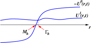
Figure 1: Illustration of $U^{0}$, $U^{1}$. Note that $U^{0}$ vanishes at $M_{h}=M(\Gamma_{0},h)$, the solution at time $h$ of MMC, starting from $M_{0}$. The intersection between $-U^{0}$ and $U^{1}$ gives $\Gamma_{h}$.

The convergence rate in (25) can in fact be improved to ${\mathcal{O}}({h}^{2})$. Estimate (25) simply makes use of the $L^{\infty}$-norm of $\big{(}\partial_{t}-\Delta\big{)}U^{0}(x,t)$. The improved rate comes by performing a more precise point-wise analysis. This will involve more analytical computation but it is quite similar to what is done in the stability estimates – see Remark 1 in Section 4.3.

2.3 Step III. Stability Estimates

Note that the consistency statement (24) involves the curvature of $\Gamma_{{h}}$. In order to ensure that such a statement can be extended to multiple iterations, we need to estimate the curvature of $\Gamma_{{h}}$ in terms of the curvature of $\Gamma_{0}$.

The first step in doing this is to describe $\Gamma_{{h}}$ as a graph over $M_{h}=M(\Gamma_{0},{h})$. This is achievable due to the fact that near $M_{h}$, we have

$$\nabla U\approx\partial_{r}U^{0}=\frac{1}{\sqrt{\pi h}}\exp\left({-\frac{r^{2}}{4h}}\right)\gg 1\,\,\,\,\,\,\text{(since $r\sim{\mathcal{O}}(h^{\frac{3}{2}})$).}$$

Hence Implicit Function Theorem (IFT) gives us that locally $\Gamma_{h}$ can be written as a graph of a function $g$ over the tangent plane $\mathbb{T}_{M_{h}}(p_{0})$ at some point $p_{0}$ on $M_{h}$ (see Figure 2). The next step is to relate the curvature of $\Gamma_{h}$ to the second derivatives of $g$.

Figure 2: The manifolds $M_{h}=M(\Gamma_{0},h)$ and $\Gamma_{h}$. Note that $d_{{\mathcal{H}}}(M_{h},\Gamma_{h})={\mathcal{O}}(h^{\frac{3}{2}})$ and $\Gamma_{h}$ locally can be written as a graph over $\mathbb{T}_{M_{h}}$: $\Gamma_{h}=\left\{{({\bar{x}},g({\bar{x}})):{\bar{x}}\in\mathbb{T}_{M_{h}}}\right\}$.

The necessary computations are also facilitated by IFT. Letting ${\mathcal{B}}_{h}$ be the Weingarten map of $\Gamma_{h}$, and $\bar{x}$ be the coordinates of the tangent plane $\mathbb{T}_{M_{h}}(p_{0})$, we have (63, 64, 65)

$${\mathcal{B}}_{h}=\nabla^{2}_{\bar{x}}g+\nabla_{\bar{x}}^{2}U^{1}{\mathcal{O}}(\sqrt{{h}})+\|{\mathcal{B}}_{0}\|^{3}{\mathcal{O}}({h}).$$ (26)

Careful analysis of $\nabla_{\bar{x}}^{2}U^{1}$ via (23) and (45) gives (Lemma 7):

$$\|\nabla_{\bar{x}}^{2}U^{1}\|_{L^{\infty}}\leq\|{\mathcal{B}}_{0}\|^{3}{\mathcal{O}}(\sqrt{{h}})$$ (27)

leading to the following one-step stability estimate (Theorem 3):

$$\|{\mathcal{B}}_{{h}}\|\leq\|{\mathcal{B}}_{0}\|+\|{\mathcal{B}}_{0}\|^{3}{\mathcal{O}}({h}).$$ (28)

The most daunting computation is the estimate (27). This is because (23) expresses $U^{1}$ in terms of higher order derivatives of $U^{0}$. The analysis thus needs to make crucial use of some regularity theory of MMC, in particular the decay estimates for the Weingarten map of $M_{t}$ (Lemmas 2 and 3).

Once we have (27), it can be iterated by means of a discrete Gronwall inequality. This leads to that the curvatures of our numerical manifolds $\Gamma_{k{h}}$ are bounded uniformly over multiple iterations of the scheme (Theorem 4).

2.4 Step IV. Convergence.

By the consistency statement and curvature bound from the previous steps, together with some geometric argument to exclude the occurrence of self-intersection, the sequence of $\Gamma_{n{h}}$ can be shown to converge to a limit manifold in the Hausdorff distance and also the $C^{1,\alpha}$-norm. The final step is to identify the equation satisfied by the limit.

We find the weak formulation of MMC using BV-functions or sets of finite perimeter as used in [27] the most convenient for our purpose. Using the notation of Theorem 1, we show that $\chi_{k{h}}$ converges to a limiting function $\chi^{*}_{t}\in BV(\mathbb{R}^{n+1};\{0,1\})$ as $k{h}\rightarrow t$. Furthermore, $\chi^{*}$ solves MMC in the sense of (12)-(13). The key step in establishing this is to prove that the area converges in the sense that

$$\int|\nabla\chi_{k{h}}|\rightarrow\int|\nabla\chi^{*}_{t}|.$$ (29)

(The above is assumed in [27].) The main ingredient in doing this is the Ball Lemma (Lemma 8) by which we may place a tubular neighborhood with uniform thickness such that $\Gamma_{k{h}}$ remains embedded.

2.5 Some notations from geometry of surfaces

The reference for this section is [10], in particular Appendix A. From our perspective and application point of view, we take the definition of the mean curvature $H$ as the negative first variation of the area functional. But for the sake of performing analytical computation, we will relate $H$ to the Weingarten map of a manifold. Essentially $H$ is defined to be the trace of the Weingarten map.

Recall that for an $n$-dimensional manifold $M=\partial\Omega$ embedded in $\mathbb{R}^{n+1}$ given by an embedding map: $M=F(D)$ where $F:D\subseteq\mathbb{R}^{n}\rightarrow\mathbb{R}^{n+1}$, the second fundamental form is the symmetric bilinear form on the tangent bundle $TM$ of $M$ given by

$$A_{ij}=\langle\partial_{i}{\mathbf{N}},\partial_{j}F\rangle=-\langle{\mathbf{N}},\partial^{2}_{ij}F\rangle$$ (30)

where ${\mathbf{N}}$ is the unit outward normal for $M$. Inherently related is the Weingarten map, which is the mapping $L$ from $TM$ to $TM$ determined by,

$$L(\mathbf{u})=-\nabla_{\mathbf{u}}{\mathbf{N}}.$$ (31)

In the coordinate system determined by $F$, the matrix corresponding to the Weingarten map is given by,

$$A^{i}_{j}=g^{ik}A_{kj},$$ (32)

where $(g^{ij})=(g_{ij})^{-1}=\big{(}\langle\partial_{i}F,\partial_{j}F\rangle\big{)}^{-1}$. The eigenvalues $\kappa_{1},\ldots,\kappa_{n}$ of $L$ are called the principal curvatures of $M$.

With the above notations, the mean curvature $H$ of $M$ is given by

$$H=\frac{1}{n}{\mbox{{\rm div}}}_{M}{\mathbf{N}}:=\frac{1}{n}\sum_{i,j}g^{ij}\langle\partial_{i}{\mathbf{N}},\partial_{j}F\rangle$$ (33)

which can be related to the trace of the Weingarten map of $M$ as follows,

$$H=\frac{1}{n}\sum_{i}A^{i}_{i}=\frac{1}{n}\left({\kappa_{1}+\cdots+\kappa_{n}}\right).$$ (34)

Of particular relevance is the case when $F$ is the graph of a function $f$ over $\mathbb{R}^{n}$, i.e. $F(x)=(x,f(x))$ for $x\in{\mathbb{R}}^{n}$. In this case, we have

$$A_{ij}=\dfrac{\nabla^{2}f}{\sqrt{1+|\nabla f|^{2}}},$$

$$(g_{ij})=I+\nabla f\otimes\nabla f,$$

and

$$(A^{i}_{j})=\left(I-\dfrac{\nabla f\otimes\nabla f}{1+|\nabla f|^{2}}\right)\dfrac{\nabla^{2}f}{\sqrt{1+|\nabla f|^{2}}}.$$ (35)

The mean curvature $H$ is then given by,

$$H=\frac{1}{n}\sum_{i=1}^{n}A_{i}^{i}=\text{div}\frac{\nabla f}{\sqrt{1+\left|{\nabla f}\right|^{2}}}.$$ (36)

For the rest of this paper, we will use $A_{M}$ (or simply $A$) to denote the Weingarten map of some general manifold $M$. But to emphasize the importance of the numerical manifolds $\Gamma_{k{h}}$’s, we will use ${\mathcal{B}}_{k{h}}$ to denote their Weingarten maps. For the analysis in the rest of the paper, we will use the following norm for the Weingarten map of a manifold $M$,

$$|A(p)|=\sqrt{\text{tr}(AA^{T})}=\sqrt{\sum_{i,j}A^{j}_{i}(p)A_{j}^{i}(p)},\,\,\,\,\,\,\text{and}\,\,\,\,\,\,\|A\|=\sup_{p\in M}|A(p)|.$$ (37)

A useful observation is that if the Weingarten map is bounded, then we can have a quantitative estimate about the size of the region over which the manifold can be written as a graph. To be specific, let $p\in M$, ${\mathbb{T}}_{p}(M)$ be its tangent plane, and locally near $p$, $f$ be the graph of $M$ over ${\mathbb{T}}_{p}(M)$. From (35), we have

$$\nabla^{2}f=\sqrt{1+|\nabla f|^{2}}\left(I+\nabla f\otimes\nabla f\right)(A^{i}_{j}).$$

Hence $\displaystyle{\left\|\nabla^{2}f\right\|\leq C\left({1+|\nabla f|^{2}}\right)^{\frac{3}{2}}\left\|A\right\|}$. Upon integrating in space, there is a universal constant $C_{*}=C_{*}(n)$ such that

$$\left\{{x\in{\mathbb{T}}_{p}(M),\,\,|{x}|\leq\frac{C_{*}}{\left\|A\right\|}}\right\}\subseteq\big{\{}x:\left|{\nabla f(x)}\right|<\infty\big{\}}.$$ (38)

The above implies that the connected component of $M\bigcap B_{\frac{C_{*}}{\left\|A\right\|}}(p)$ containing $p$ is completely given by the graph of $f$.

2.6 Time Step Size ${h}$ in Relation to the Geometry of Initial Manifold $\Gamma_{0}$

Here we discuss the requirement for the initial manifold $\Gamma_{0}$ which is a compact smooth embedded $n$-dimensional manifold in $\mathbb{R}^{n+1}$. The time step ${h}$ will be sent to zero in the convergence statement. But to be quantitative, we will specify its smallness with respect to two geometric quantities pertaining to $\Gamma_{0}$. In the following, we introduce a small constant $\delta$ such that ${h}\leq\delta$.

The first requirement is a local property. The value of $\delta$ satisfies

$$\|{\mathcal{B}}_{0}\|(\delta|\log\delta|)^{\frac{1}{4}}\leq 1.$$ (39)

The second is a more global condition. To describe this precisely, we first define the following Ball Property.

Definition 3.

Ball Property. Given an embedded n-dimensional manifold $M$ which is the boundary of a subset $\Omega\subseteq{\mathbb{R}}^{n+1}$, i.e., $M=\partial\Omega$, we say that $M$ satisfies the ball property with radius $r$ if for every $p\in M$, there are two balls $B_{r,p}^{\mbox{{\rm int}}}$ and $B_{r,p}^{\mbox{{\rm ext}}}$ (interior and exterior) with radius $r$ such that $B_{r,p}^{\mbox{{\rm int}}}\subseteq\Omega$ and $B_{r,p}^{\mbox{{\rm ext}}}\subseteq{\mathbb{R}}^{n+1}\backslash\Omega$ and

$$B_{r,p}^{\mbox{{\rm int}}}\cap M=B_{r,p}^{\mbox{{\rm ext}}}\cap M=\{{p}\}.$$ (40)

Note that the above condition is stronger than simply requiring that the curvature of $M$ is bounded from above by $\frac{1}{r}$. It is some kind of “uniform embeddedness” condition.

Now let $R(\Gamma_{0})$ be the maximal radius for which $\Gamma_{0}$ satisfies the ball property. Then we require that there is a small constant $\rho$ such that,

$$(\delta|\log\delta|)^{\frac{1}{4}}\leq\rho\leq\frac{R(\Gamma_{0})}{2}.$$ (41)

The stability analysis to be carried out in Section 4 which includes the regularity statement and the Ball Lemma will imply that for ${h}\leq\delta$ and $k={\mathcal{O}}(\frac{1}{{h}})$, we have that

$$\|{\mathcal{B}}_{k{h}}\|({h}|\log{h}|)^{\frac{1}{4}}\leq 1$$

and the $\Gamma_{k{h}}$’s will all be embedded manifolds.

The two conditions (39) and (41) will be assumed for the rest of the paper.

2.7 Notations and Conventions

Throughout the estimates in the paper, constants and bounded functions will be grouped together as $C$ and $\mathcal{O}(1)$ respectively. These are terms bounded by constants that do not depend on $\|{\mathcal{B}}_{0}\|$ or ${h}$. From one line to the next, the $C$ and $\mathcal{O}(1)$ terms may change, but we will still use $C$ and $\mathcal{O}(1)$. We will also use the following conventions:

1. $A={\mathcal{O}}(1)$ or $A(\cdot)={\mathcal{O}}(1)f(\cdot)$: there is some constant $C$ such that

   $$\left|{A}\right|\leq C\,\,\,\,\,\,\text{or}\,\,\,\,\,\,\left|{A(\cdot)}\right|\leq C\left|{f(\cdot)}\right|.$$

2. $A\lesssim B$ or $A\gtrsim B$: there is some constant $C$ such that

   $$A\leq CB\,\,\,\,\,\,\text{or}\,\,\,\,\,\,A\geq CB$$

3. $A\ll 1$ or $A\gg 1$: $A$ is a sufficiently small or large constant.

4. $A\approx B$: the following limiting behavior holds:

   $$\lim\frac{A}{B}=1.$$

   The meaning of the limit will be specified or clear from the context.

3 Ansatz and Its Consistency

In this section, we prove the consistency of the scheme by analyzing the ansatz $U^{0}$ and the error term $U^{1}=U-U^{0}$ defined in (20) and (19).

Recall that the initial manifold $\Gamma_{0}$ is a smooth, embedded $n$-dimensional manifold in ${\mathbb{R}}^{n+1}$. By the regularity of MMC, there exists a positive number $\rho=\rho(\Gamma_{0})>0$ such that for any $0<t<{h}\ll 1$, the signed distance function $r$ to $M(\Gamma_{0},t)$ is a smooth function in the $\rho$-tubular neighborhood $T_{\rho}(\Gamma_{0})$ of $\Gamma_{0}$,

$$T_{\rho}(\Gamma_{0})=\left\{{q\in{\mathbb{R}}^{n+1}:\text{dist}(q,\Gamma_{0})\leq\rho}\right\}.$$ (42)

Hence inside $T_{\rho}(\Gamma_{0})$, the $U^{0}$ and $U^{1}$ are smooth functions of $(x,t)$.

Inside $T_{\rho}(\Gamma_{0})$, we have the following representation formula for $U^{1}$ in terms of the heat kernel $G$ on $\mathbb{R}^{n+1}\times{\mathbb{R}}_{+}$ (c.f. [24]):

$$U^{1}(x,t)= \int_{0}^{t}\int_{T_{\rho}(\Gamma_{0})}G(x-y,t-\tau)\big{(}\partial_{t}-\Delta\big{)}U^{0}(y,\tau)dyd\tau$$

$$+\int_{0}^{t}\int_{\partial T_{\rho}(\Gamma_{0})}G(x-y,t-\tau)\frac{\partial U^{1}}{\partial\nu}(y,\tau)-U^{1}(y,\tau)\frac{\partial G}{\partial\nu}(x-y,t-\tau)dSd\tau.$$ (43)

where $\nu$ is the unit outward normal to $\partial T_{\rho}(\Gamma_{0})$.

We give some remarks about the above ansatz.

(i) Recall that $\rho$ is some small constant satisfying the condition (41). Hence the signed distance function to $M(\Gamma_{0},t)$, $r(\cdot,t)$, is smooth in the set $\{r(\cdot,t)<2\rho\}$ (for $0\leq t\leq{h}\leq\delta$). It will be a consequence of Lemma 8 that the same $\rho$ will work for multiple iterations, i.e. a tubular neighborhood of radius $\rho$ may be placed about $\Gamma_{k{h}}$ with the ansatz constructed in the same manner (see Theorem 4).

(ii) The second term in (43), integration on the boundary $\partial\Gamma_{\rho}(\Gamma_{0})$, produces exponentially small terms. Specifically, the following estimates hold for $U$ and $U^{0}$ on $\partial T_{\rho}(\Gamma_{0})$,

$\left|U-U^{0}\right|\lesssim e^{\frac{-\rho^{2}}{16{h}}}$,       $\left|\partial_{r}U^{0}\right|\lesssim\frac{1}{\sqrt{{h}}}e^{\frac{-\rho^{2}}{16{h}}}$,    and    $\left|\nabla U\right|\lesssim\frac{1}{\sqrt{{h}}}e^{\frac{-\rho^{2}}{8{h}}}$.

Furthermore, the area of $\partial T_{\rho}(\Gamma_{0})$ is roughly two of that of $\Gamma_{0}$. Hence we will simply omit it in our analysis.

For the following, given any constant $c$, we define $\left\{{r=c}\right\}$ to the manifold which is at a distant $c$ to $M_{t}$:

$$\left\{{r=c}\right\}=\left\{{y\in{\mathbb{R}}^{n+1}:{\mbox{{\rm sdist}}}(y,M(\Gamma_{0},t))=c}\right\}.$$ (44)

We note that for $c\ll 1$, $\left\{{r=c}\right\}$ is a smooth manifold. Let also $H_{\{r=c\}}:\left\{{r=c}\right\}\longrightarrow{\mathbb{R}}$ be the mean curvature function of $\left\{{r=c}\right\}$.

Lemma 1.

For any $(x,t)\in T_{\rho}(\Gamma_{0})\times[0,{h}]$, the following formula holds,

$$(\partial_{t}-\Delta)U^{0}(x,t)=\Big{(}H_{\{r=r(x,t)\}}(x)-H_{\{r=0\}}\big{(}\Pi(x)\big{)}\Big{)}\partial_{r}U^{0}(x,t),$$ (45)

where $\Pi(x)$ is the point in $M(\Gamma_{0},t)$ closest to $x$. In addition, we have

$$H_{\{r=r(x,t)\}}(x)-H_{\{r=0\}}(\Pi(x))=r(x,t)\psi\Big{(}r(x,t),\kappa_{1}(\Pi(x),t),\kappa_{2}(\Pi(x),t),\ldots,\kappa_{n}(\Pi(x),t)\Big{)}$$ (46)

where the $\kappa_{i}$ are the principal curvatures of $M(\Gamma_{0},t)$ evaluated at $\Pi(x)$, and

$$\psi(r,\kappa_{1},\kappa_{2},\ldots,\kappa_{n})=\sum_{i=1}^{n}\frac{\kappa_{i}^{2}}{1-r\kappa_{i}}.$$ (47)

See Figure 3 for an illustration of some of the notations appearing above.

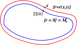
Figure 3: $\left\{{r=r(x,t)}\right\}=\left\{{y\in{\mathbb{R}}^{n+1}:{\mbox{{\rm sdist}}}(y,M(\Gamma_{0},t))=r(x,t)}\right\}$. $\Pi(x)$ is the projection of $x$ onto $M_{t}$

The above will be proved in Section A.1. We will frequently abuse the notation by simply writing $\psi(x,t)$ in place of $\psi\big{(}r(x,t),\kappa_{1}(\Pi(x),t),\kappa_{2}(\Pi(x),t),\ldots,\kappa_{n}(\Pi(x),t)\big{)}$. By the formula (22) for $\partial_{r}U^{0}$, the expression $(\partial_{t}-\Delta)U^{0}(x,t)$ takes the following form

$$\psi(r,\kappa)\dfrac{r(x,t)}{\sqrt{\pi t}}\exp\left({-\frac{r^{2}(x,t)}{4t}}\right).$$ (48)

We also note the following estimates:

$$\left\|\psi\right\|\lesssim\left\|A_{M(\Gamma_{0},t)}\right\|^{2}\,\,\,{\mbox{{\rm for}}}\,\,\,\left|{r}\right|\ll\frac{1}{\left\|A_{M(\Gamma_{0},t)}\right\|},\,\,\,\,\,\,\text{and}\,\,\,\,\,\,\left|{\frac{r}{\sqrt{t}}\exp\left({-\frac{r^{2}}{4t}}\right)}\right|={\mathcal{O}}(1)\,\,\,{\mbox{{\rm for all $r,\,t$}}}.$$ (49)

With the above, we now proceed to prove the following consistency statement for the MBO scheme.

Theorem 2.

For any ${h}\leq\delta$, there is a constant $C$ depending only on the spatial dimension such that the following estimate holds,

$$d_{\mathcal{H}}(\Gamma_{{h}},M(\Gamma_{0},{h}))\lesssim\|{\mathcal{B}}_{0}\|^{2}{h}^{\frac{3}{2}}$$ (50)

where we have used ${\mathcal{B}}_{0}$ to denote $A_{\Gamma_{0}}$.

Proof.

By (48) and (49), we have for $0<t<{h}$ that

$$\left|{(\partial_{t}-\Delta)U^{0}(x,t)}\right|=\left|{\psi(r,\kappa)\dfrac{r(x,t)}{\sqrt{\pi t}}\exp\left({-\frac{r^{2}(x,t)}{4t}}\right)}\right|\lesssim\|A_{M(\Gamma_{0},t)}\|^{2}.$$

Substituting this estimate into the integral in (43) and by the $L^{\infty}$-$L^{\infty}$ estimate of the heat operator, we obtain that,

$$\left|{U^{1}(x,{h})}\right| \leq \left|{\int_{0}^{h}\int_{T_{\rho}(\Gamma_{0})}G(x-y,{h}-\tau)\big{(}\partial_{t}-\Delta\big{)}U^{0}(y,t)dyd\tau}\right|$$

$$\leq \int_{0}^{h}\left\|G(\cdot,{h}-\tau)\right\|_{L^{1}({\mathbb{R}}^{n+1})}\left\|(\partial_{t}-\Delta)U^{0}(\cdot,\tau)\right\|_{L^{\infty}(T_{\rho}(\Gamma_{0}))}\,d\tau$$

$$\lesssim \sup_{\tau\in[0,{h}]}\|A_{M(\Gamma_{0},\tau)}\|^{2}{h}.$$

By Lemma 2 (which appears in the next section), we have

$$\sup_{t\in[0,{h}]}\|A_{M(\Gamma_{0},t)}\big{\|} \leq\big{(}\|{\mathcal{B}}_{0}\|+C\|{\mathcal{B}}_{0}\|^{3}{h}\big{)}=\|{\mathcal{B}}_{0}\|\Big{(}1+C\|{\mathcal{B}}_{0}\|^{2}{h}\Big{)}\lesssim\|{\mathcal{B}}_{0}\|$$

leading to

$$\big{\|}U^{1}(x,{h})\big{\|}_{L^{\infty}(T_{\rho}(\Gamma_{0}))}\lesssim\|{\mathcal{B}}_{0}\|^{2}{h}.$$ (51)

Finally, by the representation formula (20) of $U^{0}$, for $r\ll 1$, we have

$$U^{0}(x,t)=\frac{2}{\sqrt{\pi}}\int_{0}^{\frac{r}{2\sqrt{t}}}\exp(-y^{2})dy\approx\frac{r}{\sqrt{\pi t}}.$$ (52)

Hence $U^{0}+U^{1}$ can be zero only if $r$ satisfies

$$\left|r(\cdot,{h})\right|\lesssim\|{\mathcal{B}}_{0}\|^{2}{h}^{\frac{3}{2}}.$$

∎

4 Stability

The stability estimates of this section will allow us to extend the consistency estimate from the previous section to multiple iterations in the MBO algorithm. The first, key step is show that the curvature of $\Gamma_{{h}}$ can be controlled by the curvature of $\Gamma_{0}$. Then we prove a geometric result preventing $\Gamma_{{h}}$ to have self-intersection and hence $\Gamma_{h}$ remains embedded. Lastly, tying this together with a discrete non-linear Gronwall inequality, we are able to show that the curvatures of the $\Gamma_{k{h}}$’s are uniformly bounded over multiple iterations. The crucial computation and analysis rely on the regularity property of MMC.

We now state the two main results in this section. (We recall the notations about differential geometry from Section 2.5.)

Theorem 3.

Stability over one time step. There is a constant $C$ depending on the spatial dimension such that for ${h}\leq\delta$, we have

$$\|{\mathcal{B}}_{{h}}\|\leq\|{\mathcal{B}}_{0}\|(1+C\|{\mathcal{B}}_{0}\|^{2}{h}).$$ (53)

Theorem 4.

Stability over multiple time steps. Let $\rho$ be some small number. For any constant

$$C_{0}\in\left(\|{\mathcal{B}}_{0}\|,\min\left\{\frac{1}{(\delta|\log\delta|)^{\frac{1}{4}}},\frac{1}{2\rho}-1\right\}\right],$$ (54)

there exists a time $T=T(\Gamma_{0},C_{0})$ independent of ${h}$, such that for $0\leq k\leq\lfloor\frac{T}{{h}}\rfloor$, the following two statements hold.

• $\Gamma_{k{h}}$ is an embedded manifold. More specifically, there is a uniform radius $r_{0}=r_{0}(\Gamma_{0},C_{0})$ so that $\Gamma_{k{h}}$ satisfies the Ball Property (see Definition 3) with radius $r_{0}$.

• $\|{\mathcal{B}}_{k{h}}\|\leq C_{0}$.

(Note that for $\rho$ small enough, the interval for the choice of $C_{0}$ is non-empty which by (41) can in fact be further simplified to $\displaystyle{C_{0}\in\Big{(}\left\|{\mathcal{B}}_{0}\right\|,\frac{1}{2\rho}-1\Big{]}}$.)

Some remarks are in place.

(i) The specific manner in which $r_{0}$ and $T$ depend on $\Gamma_{0}$, and $C_{0}$ will be apparent in the proof of Theorem 4. We note also that the established curvature bound can increase with each iteration, so that the larger the choice of $C_{0}$, the larger we may choose the convergence time $T$.

(ii) Theorem 4 essentially proves that $\sup_{k}\left\|\Gamma_{k{h}}\right\|_{C^{2}}<\infty$ for appropriate range of $k$. This only implies that $\Gamma_{k{h}}$ converges in $C^{1,\alpha}$ in space. This is not sufficient to show that the convergence time $T$ for our numerical scheme coincides with the maximum time $T^{*}$ for the existence of classical solution. This is because the constant $C$ in the discrete one-time-step-stability estimate (53) might not be optimal and can be different from the continuous time case. Note however that the scaling in the growth rate of the curvature is the same in both the discrete and continuous cases as illustrated by the MMC of a circle. Finite time blow-up in the estimate over multiple time steps will definitely occur, just as in the continuous case. But the two blow-up times might not be the same. We believe that with more refined analysis, we can in fact have $\sup_{k}\left\|\Gamma_{k{h}}\right\|_{C^{2,\alpha}}<\infty$ so that the $\Gamma_{k{h}}$ converges in $C^{2,\alpha^{\prime}}$ for $\alpha^{\prime}<\alpha$, i.e. the curvature ${\mathcal{B}}_{k{h}}$ also converges (in $C^{\alpha^{\prime}}$). Then such a discrepancy between $T$ and $T^{*}$ can be removed.

As mentioned before, the proof of Theorem 3 requires some regularity results of MMC. Specifically, we need the following two lemmas for surfaces following MMC. For the next two results, we use $M_{t}$ to denote $M(M_{0},t)$, the solution of MMC starting from $M_{0}$.

Lemma 2.

Bound on Curvature Growth of MMC. There is a constant $C$ which depends only on the spatial dimension such that for $0\leq t\leq{h}$, we have

$$\|A_{M_{t}}\|\leq\|A_{M_{0}}\|(1+C\|A_{M_{0}}\|^{2}t).$$

Lemma 3.

Regularity of Higher Derivatives of MMC. Let ${\mathbf{N}}$ be the normal vector of $M_{t}$. Suppose

$$\|A_{M_{t}}\|\leq c_{0}\text{ for $t\in[0,{h}]$.}$$ (55)

Then for $t\leq{h}$, there is a constant $C$ depending on the spatial dimension such that,

$$\|\nabla_{M_{t}}A_{M_{t}}\| \leq \frac{C\cdot c_{0}}{\sqrt{t}},$$ (56)

$$\text{and}\,\,\,\,\,\,\|\partial_{t}{\mathbf{N}}\|_{L^{\infty}(M_{t})} \leq \frac{C\cdot c_{0}}{\sqrt{t}}.$$ (57)

In the above, $\|\nabla_{M_{t}}A_{M_{t}}\|=\sup_{M_{t}}\sqrt{|\nabla_{M_{t}}A_{M_{t}}|^{2}}$ where $|\nabla_{M_{t}}A_{M_{t}}|^{2}$ is the squared norm of the tensor $(\nabla_{k}A_{M_{t}})$. (See [10, Appendix A] for detail explanation of the notations.)

Note that assumption (55) holds by Lemma 2 together with assumption (39). The above Lemmas will be proved in Sections A.3 and A.4.

The stability analysis makes use of the Implicit Function Theorem (IFT). From the formula (20) and (43) for $U^{0}$ and $U^{1}$, it can be seen that,

$$\left|\partial_{r}U^{0}(x,t)\right|=\left|\frac{1}{\sqrt{\pi t}}\exp\left(-\frac{r^{2}(x,t)}{4t}\right)\right|\gtrsim\frac{1}{\sqrt{t}}\,\,\,\,\,\,\text{ for $|r(x,t)|\lesssim\sqrt{t}$,}$$

and

$$\|\nabla U^{1}(\cdot,t)\|_{L^{\infty}(T_{\rho}(\Gamma_{0}))}\lesssim\|{\mathcal{B}}_{0}\|^{2}\sqrt{t}.$$

We can then conclude that,

$$\left|\partial_{r}U(x,t)\right|>0\text{ when }\left|r(x,t)\right|\lesssim\sqrt{t}.$$

Hence, we can apply the IFT to locally write $\Gamma_{{h}}$ as the graph of a function $g$ over the tangent plane to $M(\Gamma_{0},{h})$ at some reference point (see Fig. 2).

Next we give some preparations for the proof of Theorem 3.

4.1 Further Notations and Preparations

For simplicity, we use $M_{t}$ to denote $M(\Gamma_{0},t)$ for $0<t\leq{h}$. The Weingarten maps of $M_{t}$ and $\Gamma_{h}$ are denoted by $A_{t}$ and ${\mathcal{B}}_{h}$, respectively. We further set ${\mathcal{B}}_{0}=A_{0}$.

The main goal of the next few sections is to estimate the derivatives of $U$ at any point $p\in\Gamma_{h}$. By the consistency statement, we can assume that $p\in T_{\rho}(\Gamma_{0})$. To simplify the computation, we introduce the following coordinate system. Let the origin be the point $p_{0}=\Pi_{M_{h}}(p)\in M_{h}$ which is closest to $p$. Then we write

$${\mathbb{R}}^{n+1}\cong{\mathbb{R}}^{n}\times{\mathbb{R}}\cong{\mathbb{T}}_{M_{h}}(p_{0})\times{\mathbb{L}}({\mathbf{N}}(p_{0}))$$ (58)

where ${\mathbb{T}}_{M_{h}}(p_{0})$ and ${\mathbb{L}}({\mathbf{N}}(p_{0}))$ are the tangent plane and the line spanned by the outward normal vector ${\mathbf{N}}(p_{0})$, both to $M_{h}$ at $p_{0}$. We use ${\bar{x}}\in{\mathbb{R}}^{n}$ and ${\bar{z}}\in{\mathbb{R}}$ to denote the coordinate variables of ${\mathbb{T}}_{M_{h}}(p_{0})$ and ${\mathbb{L}}({\mathbf{N}}(p_{0}))$. Then we have the following representations,

$$x=({\bar{x}},{\bar{z}})\in{\mathbb{R}}^{n+1},\,\,\,p_{0}=({\bar{x}}=0,{\bar{z}}=0),$$ (59)

and near $p_{0}$,

$$\Gamma_{h}=\left\{{({\bar{x}},g({\bar{x}})):{\bar{x}}\in{\mathbb{T}}_{M_{h}}(p_{0})}\right\},\,\,\,\text{in particular,}\,\,\,p=(0,g(0))\in{\mathbb{L}}({\mathbf{N}}(p_{0})).$$ (60)

(See Figure 2.) With the above notations, we write

$$U=U({\bar{x}},{\bar{z}},t),\,\,\,U^{0}=U^{0}({\bar{x}},{\bar{z}},t),\,\,\,U^{1}=U^{1}({\bar{x}},{\bar{z}},t),\,\,\,\text{and}\,\,\,r=r({\bar{x}},{\bar{z}},t).$$

We further note the following statements,

$$\nabla_{\bar{x}}\Big{|}_{p_{0}}=\nabla_{M_{h}}\Big{|}_{p_{0}},$$ (61)

and on ${\mathbb{L}}({\mathbf{N}}(p_{0}))$ and in particular at $p$,

$$\nabla_{\bar{x}}r=0,\,\,\,\partial_{\bar{z}}=\partial_{r},\,\,\,\partial_{\bar{z}}\nabla_{\bar{x}}r=0,\,\,\,\partial_{\bar{z}}r=-1,\,\,\,\partial_{\bar{z}}^{2}r=0.$$ (62)

We now proceed to prove Theorem 3 by estimating the derivatives of $U$ at $p$. First, by (35), ${\mathcal{B}}_{{h}}$ can be expressed in terms of $g$ via the following formula,

$${\mathcal{B}}_{{h}}=\left(I-\dfrac{\nabla_{\bar{x}}g\otimes\nabla_{\bar{x}}g}{\sqrt{1+|\nabla_{\bar{x}}g|^{2}}}\right)\dfrac{\nabla_{\bar{x}}^{2}g}{\sqrt{1+|\nabla_{\bar{x}}g|^{2}}}.$$ (63)

To analyze the above, we need the following expressions which are obtained by differentiating $g$ using the implicit function (recall that $U({\bar{x}},g({\bar{x}}),{h})=0$):

$$\nabla_{\bar{x}}g(\bar{x}) = -\frac{1}{\partial_{\bar{z}}U(\bar{x},g(\bar{x}),{h})}\nabla_{\bar{x}}U(\bar{x},g(\bar{x}),{h}),$$ (64)

$$\nabla^{2}_{\bar{x}}g(\bar{x}) = -\frac{1}{(\partial_{\bar{z}}U)}\big{(}\nabla^{2}_{\bar{x}}U+\partial_{\bar{z}}\nabla_{\bar{x}}U\otimes\nabla_{\bar{x}}g\big{)}$$ (65)

$$+\frac{1}{(\partial_{\bar{z}}U)^{2}}\big{(}\partial_{\bar{z}}\nabla_{\bar{x}}U\otimes\nabla_{\bar{x}}U+\partial_{\bar{z}\bar{z}}U\nabla_{\bar{x}}g\otimes\nabla_{\bar{x}}U\big{)}\Big{|}_{(\bar{x},g(\bar{x}),{h})}.$$

Theorem 3 is proved by obtaining precise estimates for $\nabla_{\bar{x}}g,\nabla^{2}_{{\bar{x}}}g$ and hence ${\mathcal{B}}_{{h}}$. The central technical part is the analysis of the term $\nabla_{\bar{x}}^{2}U^{1}$.

We will frequently use the following estimates concerning the Green’s function: for some constant $C$ that depend only on the spatial dimension, it holds that

$$\left\|G(\cdot,t)\right\|_{L^{1}({\mathbb{R}}^{n+1})}=1\,\,\,(\leq C)\,\,\,\text{and}\,\,\,\left\|\nabla G(\cdot,t)\right\|_{L^{1}({\mathbb{R}}^{n+1})}\leq\frac{C}{\sqrt{t}}.$$ (66)

4.2 Estimates for terms without $\nabla^{2}_{\bar{x}}U^{1}$

This section gives several preliminary estimates for various derivatives associated with $U$.

Lemma 4 (Estimates for $U^{0}$).

$$\nabla_{\bar{x}}U^{0}(p) = 0,$$ (67)

$$\nabla_{\bar{x}}^{2}U^{0}(p) = -\frac{1}{\sqrt{\pi{h}}}\exp\left(-\frac{g^{2}(0)}{4{h}}\right)\nabla^{2}_{\bar{x}}r(p)$$ (68)

$$\partial_{\bar{z}}\nabla_{\bar{x}}U^{0}(p) = 0,$$ (69)

$$\partial_{\bar{z}}U^{0}(p) = -\frac{1}{\sqrt{\pi{h}}}\exp\left(-\frac{g^{2}(0)}{4{h}}\right),$$ (70)

$$|\partial^{2}_{\bar{z}}U^{0}(p)| \lesssim \|{\mathcal{B}}_{0}\|^{2}.$$ (71)

Proof.

Recall that $\displaystyle{U^{0}=\frac{2}{\sqrt{\pi}}\int^{\frac{r}{2\sqrt{t}}}_{0}\exp(-y^{2})dy}$ and $r(x,t)=\text{sdist}(x,M_{t})$. Then we have,

$$\nabla_{{\bar{x}}}U^{0} = \frac{1}{\sqrt{\pi t}}\exp\left({-\frac{r^{2}}{4t}}\right)\nabla_{{\bar{x}}}r,$$

$$\nabla_{\bar{x}}^{2}U^{0} = \frac{1}{\sqrt{\pi t}}\left[\exp\left(-\frac{r^{2}}{4t}\right)\nabla_{\bar{x}}^{2}r+\frac{r}{2t}\exp\left(-\frac{r^{2}}{4t}\right)\nabla_{\bar{x}}r\otimes\nabla_{\bar{x}}r\right],$$

$$\partial_{\bar{z}}\nabla_{\bar{x}}U^{0} = \frac{1}{\sqrt{\pi t}}\exp\left({-\frac{r^{2}}{4t}}\right)\partial_{\bar{z}}\nabla_{{\bar{x}}}r-\frac{1}{\sqrt{\pi t}}\exp\left({-\frac{r^{2}}{4t}}\right)\frac{r}{2t}\partial_{\bar{z}}r\nabla_{{\bar{x}}}r,$$

$$\partial_{\bar{z}}U^{0} = \frac{1}{\sqrt{\pi t}}\exp\left(-\frac{r^{2}}{4t}\right)\partial_{\bar{z}}r,$$

$$\partial^{2}_{\bar{z}}U^{0} = \frac{1}{\sqrt{\pi t}}\left[{\exp\left(-\frac{r^{2}}{4t}\right)\partial_{{\bar{z}}}^{2}r-\exp\left(-\frac{r^{2}}{4t}\right)\left({\frac{r}{2t}}\right)(\partial_{\bar{z}}r)^{2}}\right]$$

Noting the property (62), and the facts $r(p)=g(0)$, and $\|g\|_{L^{\infty}}\lesssim\|{\mathcal{B}}_{0}\|^{2}{h}^{\frac{3}{2}}$ (Theorem 2), all the claims in the Lemma follow. ∎

Lemma 5 (Estimates for $U^{1}$).

$$\|\nabla U^{1}\|_{L^{\infty}(T_{\rho}(\Gamma_{0}))} \lesssim \|{\mathcal{B}}_{0}\|^{2}\sqrt{{h}},$$ (72)

$$\|\nabla^{2}U^{1}\|_{L^{\infty}(T_{\rho}(\Gamma_{0}))} \lesssim \|{\mathcal{B}}_{0}\|^{2}.$$ (73)

(In the above, the gradient operator $\nabla$ is defined with respect to the spatial variable $x\in{\mathbb{R}}^{n+1}$.)

Proof.

The statements are consequences of the $L^{1}$-estimates of the Green’s function (66).

Taking the spatial gradient in (43), we get,

$$\nabla U^{1}(x,{h})=\int_{0}^{{h}}\int_{T_{\rho}(\Gamma_{0})}\Big{(}\nabla_{y}G(x-y,{h}-\tau)\Big{)}\left(\frac{1}{\sqrt{\pi\tau}}\exp\left(-\frac{r^{2}(y,\tau)}{4\tau}\right)r(y,\tau)\psi(y,\tau)\right)dyd\tau.$$

Therefore for all $x\in T_{\rho}(\Gamma_{0})$,

$$\big{|}\nabla U^{1}(x,{h})\big{|} \lesssim\int_{0}^{{h}}\left\|\nabla G(\cdot,{h}-\tau)\right\|_{L^{1}({\mathbb{R}}^{n+1})}\left\|\frac{r(\cdot,\tau)}{\sqrt{\tau}}\exp\left(-\frac{r^{2}(\cdot,\tau)}{4\tau}\right)\psi(\cdot,\tau)\right\|_{L^{\infty}}\,d\tau$$

$$\lesssim\int_{0}^{{h}}\frac{\left\|A_{\tau}\right\|^{2}}{\sqrt{{h}-\tau}}d\tau=\|{\mathcal{B}}_{0}\|^{2}{\mathcal{O}}(\sqrt{{h}})$$

which is (72). (Note that we have used (49).)

Differentiate (43) again to get,

$$\left|\nabla^{2}U^{1}(x,{h})\right|$$

$$\leq \int_{0}^{{h}}\int_{T_{\rho}(\Gamma_{0})}\left|\nabla_{y}G(x-y,{h}-\tau)\right|\left|\nabla_{y}\left(\frac{r(y,\tau)}{\sqrt{\pi\tau}}\exp\left(-\frac{r^{2}(y,\tau)}{4\tau}\right)\psi(y,\tau)\right)\right|dyd\tau.$$

Note that for $f(y)=ye^{-\frac{y^{2}}{4}}$, we have

$$\nabla\left[{f\left({\frac{r}{\sqrt{\tau}}}\right)\psi(y,\tau)}\right]=f^{\prime}\left({\frac{r}{\tau}}\right)\frac{\nabla\tau}{\sqrt{\tau}}\psi+f\left({\frac{r}{\tau}}\right)\nabla\psi$$

so that

$$\left|{\nabla\left[{f\left({\frac{r}{\sqrt{\tau}}}\right)\psi(y,\tau)}\right]}\right|\lesssim\frac{\left\|\psi\right\|_{L^{\infty}}}{\sqrt{\tau}}+\left\|\nabla\psi\right\|_{L^{\infty}}\lesssim\frac{\left\|A_{\tau}\right\|^{2}}{\sqrt{\tau}}+\left\|A_{\tau}\nabla A_{\tau}\right\|\lesssim\frac{\left\|{\mathcal{B}}_{0}\right\|^{2}}{\sqrt{\tau}}.$$

Hence

$$\left\|\nabla^{2}U^{1}(\cdot,{h})\right\|_{L^{\infty}} \lesssim \|{\mathcal{B}}_{0}\|^{2}\int_{0}^{{h}}\frac{1}{\sqrt{{h}-\tau}}\frac{1}{\sqrt{\tau}}d\tau\,\,\,\,\,\text{(by Lemma \ref{regularity of curvature} and \eqref{GreensL1Estimates})}$$

$$\lesssim \|{\mathcal{B}}_{0}\|^{2}$$

which is (73). ∎

Lemma 6 (First derivative estimates for $U$ and $g$).

$$\big{(}\partial_{\bar{z}}U\big{)}^{-1}(p) = \left(\frac{1}{\sqrt{\pi{h}}}\exp(-\frac{g^{2}}{4{h}})\right)^{-1}\Big{(}1+\|{\mathcal{B}}_{0}\|^{2}{\mathcal{O}}({h})\Big{)},$$ (74)

$$|\nabla_{\bar{x}}g(0)| \lesssim \|{\mathcal{B}}_{0}\|^{2}{h}.$$ (75)

Proof.

First note that $\partial_{\bar{z}}U(p)=\partial_{\bar{z}}U^{0}+\partial_{\bar{z}}U^{1}$. Then by (70) and (72), we have

$$\partial_{\bar{z}}U(p) = \frac{1}{\sqrt{\pi{h}}}\exp\left({-\frac{g(0)^{2}}{4{h}}}\right)+\|{\mathcal{B}}_{0}\|^{2}{\mathcal{O}}(\sqrt{{h}})$$

$$= \frac{1}{\sqrt{\pi{h}}}\exp\left({-\frac{g(0)^{2}}{4{h}}}\right)\left({1+\sqrt{{h}}\exp\Big{(}\frac{g(0)^{2}}{4{h}}\Big{)}\|{\mathcal{B}}_{0}\|^{2}{\mathcal{O}}(\sqrt{{h}})}\right)$$

$$= \frac{1}{\sqrt{\pi{h}}}\exp\left({-\frac{g(0)^{2}}{4{h}}}\right)\Big{(}1+\|{\mathcal{B}}_{0}\|^{2}{\mathcal{O}}({h})\Big{)}$$

leading to (74). Note that we have used the estimate $\left|{g(0)}\right|\lesssim{\mathcal{O}}({h}^{\frac{3}{2}})$ from Theorem 2.

For (75), the statement follows from (64), (67), (74), and (72):

$$\left|{\nabla_{x}g}\right|=\left|{\frac{\nabla_{\bar{x}}U^{0}+\nabla_{\bar{x}}U^{1}}{\partial_{z}U}}\right| = \left|{\left\|{\mathcal{B}}_{0}\right\|^{2}{\mathcal{O}}(\sqrt{{h}})\left({\frac{1}{\sqrt{{h}}}\exp\left({-\frac{g(0)^{2}}{4{h}}}\right)}\right)^{-1}(1+\left\|{\mathcal{B}}_{0}\right\|{\mathcal{O}}({h}))}\right|$$

$$= \left|{\left\|{\mathcal{B}}_{0}\right\|^{2}{\mathcal{O}}({h})\exp\left({\frac{g(0)^{2}}{4{h}}}\right)(1+\left\|{\mathcal{B}}_{0}\right\|^{2}{h})}\right|$$

$$= \left\|{\mathcal{B}}_{0}\right\|^{2}{\mathcal{O}}({h}).$$

∎

4.3 Refined estimates for $\nabla^{2}_{\bar{x}}U^{1}$

We now begin the most substantial computation in estimating $A_{{h}}$, which is directly related to $\nabla^{2}_{\bar{x}}U^{1}$. The following is the key result of this section.

Lemma 7.

The following estimate holds,

$$\left\|\nabla_{\bar{x}}^{2}U^{1}\right\|\lesssim\|{\mathcal{B}}_{0}\|^{3}\sqrt{{h}}.$$ (76)

Before proceeding with the proof of Lemma 7, we show how Lemma 7 along with the estimates of Section 4.2 can lead to Theorem 3. First, by substituting the estimates from Lemma 5 into (65), we have

$$\nabla^{2}_{\bar{x}}g(\bar{x})\Big{|}_{(\bar{x},g(\bar{x}),{h})}$$

$$= -\frac{1}{(\partial_{\bar{z}}U)}\big{(}\nabla^{2}_{\bar{x}}U+\partial_{\bar{z}}\nabla_{\bar{x}}U\otimes\nabla_{\bar{x}}g\big{)}+\frac{1}{(\partial_{\bar{z}}U)^{2}}\Big{(}\partial_{\bar{z}}\nabla_{\bar{x}}U\otimes\nabla_{\bar{x}}U+(\partial^{2}_{{\bar{z}}}U)\nabla_{\bar{x}}g\otimes\nabla_{\bar{x}}U\Big{)}$$

$$= -\frac{1}{(\partial_{\bar{z}}U)}\big{(}\nabla^{2}_{\bar{x}}U^{0}+\nabla^{2}_{\bar{x}}U^{1}+\partial_{\bar{z}}\nabla_{\bar{x}}U^{1}\otimes\nabla_{\bar{x}}g\big{)}$$

$$+\frac{1}{(\partial_{\bar{z}}U)^{2}}\Big{(}\partial_{\bar{z}}\nabla_{\bar{x}}U^{1}\otimes\nabla_{\bar{x}}U^{1}+(\partial^{2}_{\bar{z}}U^{0}+\partial^{2}_{\bar{z}}U^{1})\nabla_{\bar{x}}g\otimes\nabla_{\bar{x}}U\Big{)}$$

$$= -\frac{1}{(\partial_{\bar{z}}U)}\left[{-\frac{1}{\sqrt{\pi{h}}}\exp\left({-\frac{g(0)^{2}}{4{h}}}\right)\nabla^{2}_{\bar{x}}r(p)+\nabla^{2}_{\bar{x}}U^{1}+\left\|{\mathcal{B}}_{0}\right\|^{2}\left\|{\mathcal{B}}_{0}\right\|^{2}{h}}\right]$$

$$+\frac{1}{(\partial_{\bar{z}}U)^{2}}\Big{(}\left\|{\mathcal{B}}_{0}\right\|^{2}\left\|{\mathcal{B}}_{0}\right\|^{2}\sqrt{{h}}+\left\|{\mathcal{B}}_{0}\right\|^{2}\left\|{\mathcal{B}}_{0}\right\|^{4}{\mathcal{O}}({h}^{\frac{3}{2}})\Big{)}$$

$$= -\left[{\frac{1}{\sqrt{\pi{h}}}\exp\left({-\frac{g(0)^{2}}{4{h}}}\right)}\right]^{-1}\left[{-\frac{1}{\sqrt{\pi{h}}}\exp\left({-\frac{g(0)^{2}}{4{h}}}\right)\nabla^{2}_{\bar{x}}r(p)+\nabla^{2}_{\bar{x}}U^{1}+\left\|{\mathcal{B}}_{0}\right\|^{4}{\mathcal{O}}({h})}\right]$$

$$+\left[{\frac{1}{\sqrt{\pi{h}}}\exp\left({-\frac{g(0)^{2}}{4{h}}}\right)}\right]^{-2}\left[{\left\|{\mathcal{B}}_{0}\right\|^{4}{\mathcal{O}}(\sqrt{{h}})+\left\|{\mathcal{B}}_{0}\right\|^{6}{\mathcal{O}}({h}^{\frac{3}{2}})}\right]$$

$$= \nabla^{2}_{\bar{x}}r(p)+\nabla^{2}_{\bar{x}}U^{1}{\mathcal{O}}(\sqrt{{h}})+\left\|{\mathcal{B}}_{0}\right\|^{4}{\mathcal{O}}({h}^{\frac{3}{2}})$$

$$= \nabla^{2}_{\bar{x}}r(p)+\left\|{\mathcal{B}}_{0}\right\|^{3}{\mathcal{O}}({h})+\left\|{\mathcal{B}}_{0}\right\|^{4}{\mathcal{O}}({h}^{\frac{3}{2}}).$$

Now apply the above to (63) which relates ${\mathcal{B}}_{h}$ to $\nabla_{\bar{x}}^{2}g$, we get

$$|{\mathcal{B}}_{{h}}| = \frac{\left|{\text{tr}\big{(}\nabla_{\bar{x}}^{2}g\big{)}}\right|}{\sqrt{1+\left|{\nabla_{\bar{x}}g}\right|^{2}}}\left|{I-\frac{\nabla_{\bar{x}}g\otimes\nabla_{\bar{x}}g}{\sqrt{1+\left|{\nabla_{\bar{x}}g}\right|^{2}}}}\right|$$

$$\lesssim \Big{(}\left|{\triangle_{\bar{x}}r(p)}\right|+\left\|{\mathcal{B}}_{0}\right\|^{3}{\mathcal{O}}({h})+\left\|{\mathcal{B}}_{0}\right\|^{4}{\mathcal{O}}({h}^{\frac{3}{2}})\Big{)}\left({1+C\left\|{\mathcal{B}}_{0}\right\|^{2}{\mathcal{O}}({h}^{2})}\right)$$

$$\lesssim \Big{(}\left|{H_{\left\{{r=r(p)}\right\}}(p)}\right|+\left\|{\mathcal{B}}_{0}\right\|^{3}{\mathcal{O}}({h})+\left\|{\mathcal{B}}_{0}\right\|^{4}{\mathcal{O}}({h}^{\frac{3}{2}})\Big{)}\left({1+C\left\|{\mathcal{B}}_{0}\right\|^{2}{\mathcal{O}}({h}^{2})}\right)$$

$$\lesssim \Big{(}\left\|A_{h}\right\|+\left\|{\mathcal{B}}_{0}\right\|^{3}{\mathcal{O}}({h})+\left\|{\mathcal{B}}_{0}\right\|^{4}{\mathcal{O}}({h}^{\frac{3}{2}})\Big{)}\left({1+C\left\|{\mathcal{B}}_{0}\right\|^{2}{\mathcal{O}}({h}^{2})}\right)$$

$$\lesssim \Big{(}\left\|{\mathcal{B}}_{0}\right\|(1+C\left\|{\mathcal{B}}_{0}\right\|^{2}{\mathcal{O}}({h}))+\left\|{\mathcal{B}}_{0}\right\|^{3}{\mathcal{O}}({h})+\left\|{\mathcal{B}}_{0}\right\|^{4}{\mathcal{O}}({h}^{\frac{3}{2}})\Big{)}\left({1+C\left\|{\mathcal{B}}_{0}\right\|^{2}{\mathcal{O}}({h}^{2})}\right)$$

$$\lesssim \left\|{\mathcal{B}}_{0}\right\|\left({1+C\left\|{\mathcal{B}}_{0}\right\|^{2}{\mathcal{O}}({h})}\right)$$

which is the statement of Theorem 3. In the above, $\triangle_{\bar{x}}r(p)=H_{\left\{{r=r(p)}\right\}}(p)$ is the mean curvature of the manifold $\left\{{r=r(p,{h})}\right\}$ at $p$. It is estimated in terms of $\left\|A_{h}\right\|$ by using (118):

$$\left|{H_{\left\{{r=r(p,{h})}\right\}}(p)}\right|=\left|{\sum_{i}\frac{\kappa_{i}(\Pi(p))}{1-r(p,{h})\kappa_{i}(\Pi(p))}}\right|\leq\left\|A_{h}\right\|\left({1+\left\|A_{h}\right\|{\mathcal{O}}({h}^{\frac{3}{2}})}\right)$$

and then in terms of $\left\|{\mathcal{B}}_{0}\right\|$ by using Lemma 2.

The proof of Lemma 7 is divided into several sub-sections.

4.3.1 Preparation for Estimating $\nabla_{\bar{x}}^{2}U^{1}(p,{h})$, $p\in\Gamma_{h}$

Evaluating $U^{1}(x,t)$ at $x=p=(0,g(0))$ and $t={h}$, we get,

$$U^{1}(p,{h}) =-\int_{0}^{{h}}\int_{T_{\rho}(\Gamma_{0})}G(p-y,{h}-\tau)\psi(y,\tau)\dfrac{r(y,\tau)}{\sqrt{\pi\tau}}\exp\left(-\frac{r^{2}(y,\tau)}{4\tau}\right)dyd\tau.$$

For the integration in the $y$ variable, we use the coordination system (58) (see also Figure 2):

$${\mathbb{R}}^{n+1}\cong{\mathbb{R}}^{n}\times{\mathbb{R}}\cong\left\{{(y_{1},y_{2},\ldots y_{n})\in{\mathbb{R}}^{n}}\right\}\times\left\{{y_{n+1}\in{\mathbb{R}}}\right\}.$$ (77)

Taking the second partial derivatives in tangential directions ${\bar{x}}_{i}$ and ${\bar{x}}_{j}$ for $1\leq i,j\leq n$ leads to

$$\partial^{2}_{{\bar{x}}_{i}{\bar{x}}_{j}}U^{1}(p,{h})\\ =-\int_{0}^{{h}}\int_{T_{\rho}(\Gamma_{0})}\Big{(}\partial_{y_{j}}G(p-y,{h}-\tau)\Big{)}\partial_{y_{i}}\left[{\psi(y,\tau)\dfrac{r(y,\tau)}{\sqrt{\tau}}\exp\left(-\frac{r^{2}(y,\tau)}{4\tau}\right)}\right]dyd\tau.$$ (78)

In addition, for $\left|x-y\right|\geq\sqrt{2(n+5)({h}-\tau)\left|\log({h}-\tau)\right|}$, we have

$$\left|\nabla G(x-y,{h}-\tau)\right|\leq\frac{1}{2\left(4\pi\right)^{\frac{n+1}{2}}}\left({h}-\tau\right)^{\frac{3}{2}}\sqrt{({h}-\tau)\left|\log({h}-\tau)\right|}=o({h}).$$

Hence we can restrict our analysis of (78) to the following region

$$\Big{\{}y\in{\mathbb{R}}^{n+1}:|p-y|\leq\sqrt{2(n+5){h}|\log{h}|}\Big{\}}.$$ (79)

Now we compute:

$$\partial_{y_{i}}\left[{\psi(y,\tau)\dfrac{r(y,\tau)}{\sqrt{\pi\tau}}\exp\left({-\frac{r^{2}(y,\tau)}{4\tau}}\right)}\right]$$ (81)

$$= \psi(y,\tau)\left({1-\frac{r^{2}(y,\tau)}{2\tau}}\right)\exp\left({-\frac{r^{2}(y,\tau)}{4\tau}}\right)\frac{\partial_{y_{j}}r}{\sqrt{\pi\tau}}$$

$$+\dfrac{r(y,\tau)}{\sqrt{\pi\tau}}\exp\left({-\frac{r^{2}(y,\tau)}{4\tau}}\right)\partial_{y_{i}}\psi(y,\tau)$$

Then we decompose (78) into the following two terms:

$$\partial^{2}_{x_{i}x_{j}}U^{1}(0,g(0))=-I-J$$

where

$$I = -\int_{0}^{{h}}\int_{T_{\rho}(\Gamma_{0})}\partial_{y_{j}}\Big{(}G(p-y,{h}-\tau)\Big{)}\Big{(}{\text{expression \eqref{I.def}}}\Big{)}\,dyd\tau,$$ (82)

$$J = -\int_{0}^{{h}}\int_{T_{\rho}(\Gamma_{0})}\partial_{y_{j}}\Big{(}G(p-y,{h}-\tau)\Big{)}\Big{(}{\text{expression \eqref{J.def}}}\Big{)}\,dyd\tau.$$ (83)

Observe that $I$ does not involve any derivatives of the curvature term, while $J$ does.

The main estimates we will arrive at are:

$$\left|{I}\right|\lesssim\|{\mathcal{B}}_{0}\|^{3}\sqrt{{h}}\,\,\,\,\,\,\text{and}\,\,\,\,\,\,\left|{J}\right|\lesssim\|{\mathcal{B}}_{0}\|^{3}\sqrt{{h}}$$

which together will give the result of Lemma 7.

4.3.2 Analysis of $I$ (82), term without derivatives of curvature

Note that

$$\partial_{y_{i}}r(y,\tau)=\left\langle{{\mathbf{N}}(M_{\tau},\Pi_{M_{\tau}}y)},\,{{\mathbf{E}}_{i}}\right\rangle$$ (84)

where

$$\Pi_{M}(y) = M y$$ closest point on to ,

$${\mathbf{N}}(M,q) = M q\in M$$ (outward) normal vector to at .

$${\mathbf{E}}_{i} = i {\mathbb{T}}_{M_{h}}(p_{0})$$ the -th coordinate vector of .

We will also use the following abbreviation,

$$\Pi_{\tau}(y)=\Pi_{M_{\tau}}(y),\,\,\,\,\,\,{\mathbf{N}}_{\tau}(y)={\mathbf{N}}(M_{\tau},\Pi_{M_{\tau}}(y)).$$

The main observation is that ${\mathbf{N}}_{\tau}(y)\approx{\mathbf{N}}_{h}(p)$ which is orthogonal to ${\mathbf{E}}_{i}$ for $i=1,2,\ldots n$. This is made precise as follows. First extend the normal vector to $M_{\tau}$ as a vector field over $T_{\rho}(\Gamma_{0})$ by taking it to be constant in directions normal to $M_{\tau}$. Let $\nabla$ be the gradient operator on $\mathbb{R}^{n+1}$. Then

$${\mathbf{N}}_{\tau}(y) = {\mathbf{N}}_{h}(p)+\int_{0}^{1}\nabla{\mathbf{N}}_{\tau}(y+\lambda(p-y))(p-y)\,d\lambda-\int_{\tau}^{h}\frac{d}{ds}{\mathbf{N}}_{s}(y)\,ds$$

$$= {\mathbf{N}}_{h}(p)+\mathcal{O}(1)\|{\mathcal{B}}_{0}\|\left(({h}-\tau)^{\frac{1}{2}}+|p-y|\right)\,\,\,\,\,\,\text{(by Lemma \ref{regularity of curvature})}$$

which leads to

$$\Big{|}\left\langle{{\mathbf{N}}_{\tau}(y)},\,{{\mathbf{E}}_{i}}\right\rangle\Big{|}\lesssim\|{\mathcal{B}}_{0}\|\left(({h}-\tau)^{\frac{1}{2}}+|p-y|\right).$$ (85)

Substituting the above into $I$ (82), we get

$$\left|{I}\right| = \left|\int_{0}^{{h}}\int_{T_{\rho}(\Gamma_{0})}\Big{(}\partial_{y_{j}}G(p-y,{h}-\tau)\Big{)}\psi(y,t)\times\right.$$

$$\left.\times\Big{(}1-\frac{r^{2}(y,\tau)}{2\tau}\Big{)}\exp\left(-\frac{r^{2}(y,\tau)}{4\tau}\right)\frac{\left\langle{{\mathbf{N}}_{\tau}},\,{{\mathbf{E}}_{i}}\right\rangle}{\sqrt{\tau}}\,dy\,d\tau\right|$$

$$\lesssim \left|{\int_{0}^{h}\int_{T_{\rho}(\Gamma_{0})}\left|{\nabla_{y}G(p-y,{h}-\tau)}\right|\left\|\psi\right\|_{L^{\infty}}\frac{\|{\mathcal{B}}_{0}\|\left(({h}-\tau)^{\frac{1}{2}}+|p-y|\right)}{\sqrt{\tau}}\,dy\,d\tau}\right|$$

$$\lesssim \|{\mathcal{B}}_{0}\|^{3}\left|{\int_{0}^{h}\int_{T_{\rho}(\Gamma_{0})}\left|{\nabla_{y}G(p-y,{h}-\tau)}\right|\frac{\left(({h}-\tau)^{\frac{1}{2}}+|p-y|\right)}{\sqrt{\tau}}\,dy\,d\tau}\right|.$$

Now for

$$\left|{\int_{0}^{h}\int_{T_{\rho}(\Gamma_{0})}\left|{\nabla_{y}G(p-y,{h}-\tau)}\right|\frac{({h}-\tau)^{\frac{1}{2}}}{\sqrt{\tau}}\,dy\,d\tau}\right|$$

$$\lesssim \left|{\int_{0}^{h}\left\|\nabla G(\cdot,{h}-\tau)\right\|_{L^{1}({\mathbb{R}}^{n+1})}\frac{({h}-\tau)^{\frac{1}{2}}}{\sqrt{\tau}}\,dy\,d\tau}\right|\lesssim\int_{0}^{h}\frac{1}{\sqrt{\tau}}\,d\tau={\mathcal{O}}(\sqrt{{h}}),$$

while for

$$\left|{\int_{0}^{h}\int_{T_{\rho}(\Gamma_{0})}\left|{\nabla_{y}G(p-y,{h}-\tau)}\right|\frac{|{p-y}|}{\sqrt{\tau}}\,dy\,d\tau}\right|$$

$$\lesssim \left|{\int_{0}^{h}\int_{{\mathbb{R}}^{n+1}}\frac{1}{({h}-\tau)^{\frac{n+1}{2}}}\exp\left(-\frac{|{y}|^{2}}{4({h}-\tau)}\right)\frac{|{y}|}{{h}-\tau}\frac{|{y}|}{\sqrt{\tau}}\,dy\,d\tau}\right|$$

$$\lesssim \left|{\int_{0}^{h}\int_{{\mathbb{R}}^{n+1}}\exp\left(-\frac{|{y}|^{2}}{4}\right)|{y}|^{2}\frac{1}{\sqrt{\tau}}\,dy\,d\tau}\right|\lesssim\left|{\int_{0}^{h}\frac{1}{\sqrt{\tau}}\,d\tau}\right|={\mathcal{O}}(\sqrt{{h}})$$

which combined together gives the estimate for $I$ stated in (82).

4.3.3 Analysis of $J$ (83), term involving derivatives of curvature

Recall the formula (47) for the function $\psi$ where the curvatures are evaluated at $\Pi_{\tau}(y)$. Then we have

$$\partial_{y_{j}}\psi = \sum_{l}^{n}\partial_{y_{j}}\left({\frac{\kappa_{l}^{2}}{1-r\kappa_{l}}}\right)$$

$$= 2\sum_{l=1}^{n}\frac{\kappa_{l}\partial_{y_{i}}\kappa_{l}}{1-r\kappa_{l}}+\sum_{l=1}^{n}\frac{\kappa_{l}^{2}}{(1-r\kappa_{l})^{2}}\Big{(}r\partial_{y_{i}}\kappa_{l}+\kappa_{l}\partial_{y_{j}}r\Big{)}$$

$$= 2\sum_{l=1}^{n}\kappa_{l}\partial_{y_{i}}\kappa_{l}+\sum_{l=1}^{n}\left[r\left(\frac{2\kappa_{l}^{2}\partial_{y_{i}}\kappa_{l}}{1-r\kappa_{l}}+\kappa_{l}^{2}\frac{\partial_{y_{i}}\kappa_{l}}{(1-r\kappa_{l})^{2}}\right)+\frac{\kappa_{l}^{3}\langle{\mathbf{N}}_{\tau}(y),{\mathbf{E}}_{i}\rangle}{(1-r\kappa_{l})^{2}}\right]$$

$$= 2\sum_{l=1}^{n}\kappa_{l}\partial_{y_{j}}\kappa_{l}+\mathcal{O}(1)\|{\mathcal{B}}_{0}\|^{3}\left[\frac{r}{\sqrt{t}}+\|{\mathcal{B}}_{0}\|(|x_{0}-y|+|{h}-t|^{\frac{1}{2}})\right],$$

where (85) and Lemma 3 have been used. Substituting this back into (83), we obtain,

$$-J = 2\int_{0}^{{h}}\int_{T_{\rho}(\Gamma_{0})}\partial_{y_{j}}G(p-y,{h}-\tau)\left[\dfrac{r(y,\tau)}{\sqrt{\tau}}\exp\left(-\frac{r^{2}(y,\tau)}{4\tau}\right)\sum_{l=1}^{n}\kappa_{l}\partial_{y_{i}}\kappa_{l}\right]dyd\tau$$

$$+\int_{0}^{{h}}\int_{T_{\rho}(\Gamma_{0})}\partial_{y_{j}}G(p-y,{h}-\tau)\left[\dfrac{r(y,\tau)}{\sqrt{\tau}}\exp\left(-\frac{r^{2}(y,\tau)}{4\tau}\right)\times\right.$$

$$\hskip 80.0pt\left.\times\mathcal{O}(1)\|{\mathcal{B}}_{0}\|^{3}\left({\frac{r(y,\tau)}{\sqrt{\tau}}+\|{\mathcal{B}}_{0}\|\left({|p-y|+|{h}-\tau|^{\frac{1}{2}}}\right)}\right)\right]dyd\tau$$

$$:= J_{1}+J_{2}.$$

Note that both $J_{1}$ and $J_{2}$ contains derivatives of $\kappa_{l}$’s. However, $J_{2}$ is easier to deal with as it contains the pre-factor $r$ which makes the integrand small. Hence it is analyzed first.

Analysis of $J_{2}$ (4.3.3). Notice that,

$$\dfrac{r(y,\tau)}{\sqrt{\tau}}\exp(-\frac{r^{2}(y,\tau)}{4\tau})\|{\mathcal{B}}_{0}\|^{3}\left[\frac{r(y,\tau)}{\sqrt{\tau}}+\|{\mathcal{B}}_{0}\|(|p-y|+|{h}-\tau|^{\frac{1}{2}})\right]$$

$$\lesssim \frac{r^{2}}{\tau}\exp\left({-\frac{r^{2}}{4\tau}}\right)\|{\mathcal{B}}_{0}\|^{3}+\|{\mathcal{B}}_{0}\|^{4}\frac{r}{\sqrt{\tau}}\exp\left({-\frac{r^{2}}{\sqrt{4\tau}}}\right)(|p-y|+|{h}-\tau|^{\frac{1}{2}})$$

$$\lesssim \|{\mathcal{B}}_{0}\|^{3}+\|{\mathcal{B}}_{0}\|^{4}(|p-y|+|{h}-\tau|^{\frac{1}{2}}).$$

Hence

$$|J_{2}| \lesssim \int_{0}^{h}\int_{{\mathbb{R}}^{n+1}}\left|{\nabla G(\cdot,{h}-\tau)}\right|\left[{\|{\mathcal{B}}_{0}\|^{3}+\|{\mathcal{B}}_{0}\|^{4}(|p-y|+|{h}-\tau|^{\frac{1}{2}})}\right]$$

$$\lesssim \|{\mathcal{B}}_{0}\|^{3}\sqrt{{h}}+\|{\mathcal{B}}_{0}\|^{4}{h}\lesssim\|{\mathcal{B}}_{0}\|^{3}\sqrt{{h}}.$$

Analysis of $J_{1}$ (4.3.3). First note that the following simple bound for $J_{1}$

$$\left|{J_{1}}\right| \lesssim \left|{\int_{0}^{{h}}\int_{T_{\rho}(\Gamma_{0})}\partial_{y_{j}}G(p-y,{h}-\tau)\left[\dfrac{r(y,\tau)}{\sqrt{\tau}}\exp\left(-\frac{r^{2}(y,\tau)}{4\tau}\right)\sum_{l=1}^{n}\kappa_{l}\partial_{y_{i}}\kappa_{l}\right]dyd\tau}\right|$$

$$\lesssim \left|{\int_{0}^{h}\left\|\nabla G(\cdot,{h}-\tau)\right\|_{L^{1}({\mathbb{R}}^{n+1})}\frac{\left\|{\mathcal{B}}_{0}\right\|^{2}}{\sqrt{\tau}}\,dy\,d\tau}\right|$$

$$\lesssim \left\|{\mathcal{B}}_{0}\right\|^{2}\int_{0}^{h}\frac{1}{\sqrt{{h}-\tau}}\frac{1}{\sqrt{\tau}}\,d\tau\lesssim\left\|{\mathcal{B}}_{0}\right\|^{2}$$

is too crude for our purpose. The following more refined computation takes into account the different scalings of the integrand along the tangential and normal directions to $M_{\tau}$.

For this purpose, we will use the co-area formula to perform the integration in $J_{1}$ over $\left\{{r=r^{\prime}}\right\}$ for $-\rho\leq r^{\prime}\leq\rho$:

$$J_{1}=2\int_{0}^{{h}}\int_{-\rho}^{\rho}\int_{\{r=r^{\prime}\}}\Big{(}\partial_{y_{j}}G(p-y,{h}-\tau)\Big{)}\Big{(}\dfrac{r^{\prime}(y,\tau)}{\sqrt{\tau}}\exp(-\frac{r^{\prime 2}(y,\tau)}{4\tau})\Big{)}\Big{(}\sum_{l=1}^{n}\kappa_{l}\partial_{x_{i}}\kappa_{l}\Big{)}_{\Pi_{\tau}(y)}\times\\ \times dA_{r^{\prime}}(y)dr^{\prime}d\tau.$$

In the above, we recall the sign distance function $r$ (18) to $M_{\tau}$ and the notation (44) $\left\{{r=r^{\prime}}\right\}=\left\{{y\in{\mathbb{R}}^{n+1}:r(y,\tau)=r^{\prime}}\right\}$. Furthermore, $dA_{r^{\prime}}$ is the volume form of $\left\{{r=r^{\prime}}\right\}$. Then we parametrize the collection of manifolds $\Big{\{}\left\{{r=r^{\prime}}\right\}:-\rho\leq r^{\prime}\leq\rho\Big{\}}$ using $M_{\tau}$ as follows:

$$\tilde{s}:\,\,\,M_{\tau}\times(-\rho,\rho)\longrightarrow\tilde{s}(s,r^{\prime}):=s+r^{\prime}{\mathbf{N}}(s,\tau)$$ (88)

where ${\mathbf{N}}(s,\tau)$ is the unit normal to $M_{\tau}$ at $s$. Note that $s=\Pi_{\tau}(\tilde{s})$. Then

$$J_{1}=2\int_{0}^{{h}}\int_{-\rho}^{\rho}\int_{M_{\tau}}\partial_{y_{j}}\Big{(}G(p-\tilde{s},{h}-\tau)\Big{)}\Big{(}\sum_{l=1}^{n}\kappa_{l}(s,\tau)\partial_{y_{i}}\kappa_{l}(s,\tau)\Big{)}\dfrac{r^{\prime}}{\sqrt{\tau}}\exp(-\frac{r^{\prime 2}}{4\tau})\times\\ \times\left|{\frac{dA_{r^{\prime}}(\tilde{s})}{dA_{0}(s)}}\right|dA_{0}(s)\,dr^{\prime}\,d\tau$$

where $dA_{0}$ is the volume form of $M_{\tau}$ and $\left|{\frac{dA_{r^{\prime}}(\tilde{s})}{dA_{0}(s)}}\right|$ is Jacobian for the change of variable from $\tilde{s}\in\left\{{r=r^{\prime}}\right\}$ to $s\in M_{\tau}$.

Next we decompose

$$J_{1}=J_{11}+J_{12}$$

where

$$J_{11}=2\int_{0}^{{h}}\int_{-\rho}^{\rho}\int_{M_{\tau}}\partial_{y_{j}}\Big{(}G(p-\tilde{s},{h}-\tau)\Big{)}\Big{(}\sum_{l=1}^{n}\kappa_{l}(s,\tau)\partial_{y_{i}}\kappa_{l}(s,\tau)\Big{)}\dfrac{r^{\prime}}{\sqrt{\tau}}\exp(-\frac{r^{\prime 2}}{4\tau})\times\\ \times dA_{0}(s)\,dr^{\prime}\,d\tau,$$ (89)

and

$$J_{12}=2\int_{0}^{{h}}\int_{-\rho}^{\rho}\int_{M_{\tau}}\partial_{y_{j}}\Big{(}G(p-\tilde{s},{h}-\tau)\Big{)}\Big{(}\sum_{l=1}^{n}\kappa_{l}(s,\tau)\partial_{y_{i}}\kappa_{l}(s,\tau)\Big{)}\dfrac{r^{\prime}}{\sqrt{\tau}}\exp(-\frac{r^{\prime 2}}{4\tau})\times\\ \times\left[{\left|{\frac{dA_{r^{\prime}}(\tilde{s})}{dA_{0}(s)}}\right|-1}\right]dA_{0}(s)\,dr^{\prime}\,d\tau.$$ (90)

In a sense, $J_{12}$ is the error term due to the deviation of the Jacobian from $1$. Hence $J_{11}$ is the dominating term. The remainder of this subsection is to show that both $|J_{11}|$ and $|J_{12}|$ can be bounded from above by $C\left\|{\mathcal{B}}_{0}\right\|\sqrt{{h}}$.

To proceed, we decompose $\nabla G$ into two exponential kernels, corresponding to integrating in the tangential and normal directions to $M_{\tau}$. For this purpose, we introduce the operator $\Sigma_{s,\tau}(p)$ which gives the orthogonal projection of $p$ onto $\text{Span}\left\{{{\mathbf{N}}(s,\tau)}\right\}$, the normal line at $s\in M_{\tau}$. (See Figure 4.)

Figure 4: Illustration of $\Sigma_{s,\tau}$. Note that for any $\tilde{s}\in T_{\rho}(\Gamma_{0})$, it can be decomposed as $\tilde{s}=s+(\tilde{s}-s)$ where $s=\Pi_{\tau}(\tilde{s})\in M_{\tau}$ and $\tilde{s}-s\in\text{Span}({\mathbf{N}}(s,\tau))$.

Then for any $\tilde{s}=s+r^{\prime}{\mathbf{N}}(s,\tau)\in\left\{{r=r^{\prime}}\right\}$, we write,

$$p-\tilde{s}=\big{[}p-\Sigma_{s,\tau}(p)\big{]}+\big{[}\Sigma_{s,\tau}(p)-\tilde{s}\big{]}.$$ (91)

Note that

$$\partial_{y_{j}}G(p-y,{h}-\tau)=\frac{1}{({h}-\tau)^{\frac{n+1}{2}}}\exp\left({-\frac{|{p-y}|^{2}}{4({h}-\tau)}}\right)\frac{\left\langle{p-y},\,{{\mathbf{E}}_{j}}\right\rangle}{{h}-\tau}.$$

Hence

$$\partial_{y_{j}}G(p-\tilde{s},{h}-\tau)$$

$$= \left[{\frac{\langle p-\Sigma_{s,\tau}(p),{\mathbf{E}}_{j}\rangle}{({h}-\tau)^{\frac{n+1}{2}+1}}+\frac{\langle\Sigma_{s,\tau}(p)-\tilde{s},{\mathbf{E}}_{j}\rangle}{({h}-\tau)^{\frac{n+1}{2}+1}}}\right]\exp\left({-\frac{|p-\Sigma_{s,\tau}(p)|^{2}}{4({h}-\tau)}}\right)\exp\left({-\frac{|\Sigma_{s,\tau}(p)-\tilde{s}|^{2}}{4({h}-\tau)}}\right).$$

Substituting the above into the expression for $J_{11}$, we have

$$J_{11}=J_{111}+J_{112}$$

where

$$J_{111} = \int_{0}^{{h}}\int_{M_{\tau}}\frac{\langle p-\Sigma_{s,\tau}(p),{\mathbf{E}}_{j}\rangle}{({h}-\tau)^{\frac{n}{2}+1}}\exp\left({-\frac{|p-\Sigma_{s,\tau}(p)|^{2}}{4({h}-\tau)}}\right)\left({\sum_{l=1}^{n}\kappa_{l}\partial_{y_{i}}\kappa_{l}}\right)_{(s,\tau)}\times$$

$$\times\left[{\frac{1}{({h}-\tau)^{\frac{1}{2}}}\int_{r^{\prime}}\exp\left({-\frac{|\Sigma_{s,\tau}(p)-\tilde{s}|^{2}}{4({h}-\tau)}}\right)\frac{r^{\prime}}{\sqrt{\tau}}\exp(-\frac{r^{\prime 2}}{4\tau})dr^{\prime}}\right]dA_{0}(s)\,d\tau,$$

$$J_{112} = \int_{0}^{{h}}\int_{M_{\tau}}\frac{1}{({h}-\tau)^{\frac{n}{2}}}\exp\left({-\frac{|p-\Sigma_{s,t}(p)|^{2}}{4({h}-\tau)}}\right)\left({\sum_{l=1}^{n}\kappa_{l}\partial_{x_{i}}\kappa_{l}}\right)_{(s,\tau)}\times$$

$$\times\left[{\frac{1}{({h}-\tau)^{\frac{1}{2}}}\int_{r^{\prime}}\frac{\langle\Sigma_{s,t}(p)-\tilde{s},{\mathbf{E}}_{j}\rangle}{({h}-\tau)}\exp\left({-\frac{|\Sigma_{s,t}(p)-\tilde{s}|^{2}}{4({h}-\tau)}}\right)\frac{r^{\prime}}{\sqrt{\tau}}\exp(-\frac{r^{\prime 2}}{4\tau})dr^{\prime}}\right]dA_{0}(s)\,d\tau.$$

which essentially correspond to integrations along the tangential and normal directions.

Analysis of $J_{111}$. We first evaluate the inner integration with respect to $r^{\prime}$. From Section A.2, we have that,

$$\frac{1}{({h}-\tau)^{\frac{1}{2}}}\int_{-\infty}^{\infty}\exp\left({-\frac{|\Sigma_{s,\tau}(p)-\tilde{s}|^{2}}{4({h}-\tau)}}\right)\frac{r^{\prime}}{\sqrt{\tau}}\exp\left({-\frac{r^{\prime 2}}{4\tau}}\right)dr^{\prime}\\ =2\sqrt{\pi}\frac{\tau}{{h}^{\frac{3}{2}}}r(\Sigma_{s,t}(p),\tau)\exp\left({-\frac{r^{2}(\Sigma_{s,\tau}(p),\tau)}{4{h}}}\right).$$ (92)

Substituting this into $J_{111}$, we get

$$J_{111}=\frac{\sqrt{\pi}}{({h})^{\frac{3}{2}}}\int_{0}^{{h}}\tau\left[\int_{M_{\tau}}\frac{\langle p-\Sigma_{s,\tau}(p),{\mathbf{E}}_{j}\rangle}{({h}-\tau)^{\frac{n}{2}+1}}\exp\left({-\frac{|p-\Sigma_{s,\tau}(p)|^{2}}{4({h}-\tau)}}\right)\left({\sum_{l=1}^{n}\kappa_{l}\partial_{y_{i}}\kappa_{l}}\right)_{(s,\tau)}\right.\times\\ \left.\times r(\Sigma_{s,\tau}(p),\tau)\exp\left({-\frac{r^{2}(\Sigma_{s,\tau}(p),\tau)}{4{h}}}\right)dA_{0}(s)\right]d\tau.$$ (93)

Heuristically, the inner integration on $M_{\tau}$ is essentially a convolution with the $n$-dim Green’s function integrated on the tangent plane ${\mathbb{T}}_{M_{\tau}}(p_{0})$ to $M_{\tau}$ at $p_{0}=\Pi_{M_{\tau}}(p)$. Recall the coordinate system (77). Note also that by (78), we may restrict our attention to $|y|\leq\sqrt{2(n+5){h}|\log{h}|}\ll 1$. Now we change the integration variable from $s$ to $y$. The following estimates can be established,

$$\exp\left({-\dfrac{|p-\Sigma_{s,\tau}(p)|^{2}}{4({h}-\tau)}}\right) \lesssim \exp\left(-\dfrac{C|y|^{2}}{{h}-\tau}\right)$$ (94)

$$|p-\Sigma_{s,\tau}(p)| \lesssim |y|,$$ (95)

$$dA_{0} \lesssim d^{n}y.$$ (96)

We further note the following two statements:

1. Let $f$ be the graph of $M_{\tau}$ over ${\mathbb{T}}_{M_{\tau}}(p_{0})$. Then

   $$\big{|}r(\Sigma_{s,\tau}(p),\tau)\big{|} \lesssim \left|{r(p,\tau)}\right|+\left|{\langle y,\nabla f\rangle}\right|\lesssim\left|{r(p,\tau)}\right|+\left|{y}\right|\left|{\nabla f}\right|$$

   $$\lesssim \|{\mathcal{B}}_{0}\|^{2}{h}^{\frac{3}{2}}+\|{\mathcal{B}}_{0}\|^{2}{h}\left|{y}\right|$$

   $$\lesssim \|{\mathcal{B}}_{0}\|^{2}{h}^{\frac{3}{2}}+\|{\mathcal{B}}_{0}\|^{2}({h}^{2}+\left|{y}\right|^{2}).$$

2. By the regularity estimate Lemma 3 for MMC, we have

   $$|\nabla_{y_{i}}\kappa_{l}|\lesssim\frac{\|B_{\tau}\|}{\sqrt{\tau}}\lesssim\frac{\|B_{0}\|}{\sqrt{\tau}}.$$ (97)

Now substituting (94) - (97) into (93), we obtain,

$$|J_{111}|\lesssim\frac{1}{{h}^{\frac{3}{2}}}\int_{0}^{{h}}\tau\int_{y}\frac{|y|}{({h}-\tau)^{\frac{n}{2}+1}}\exp\left({-\frac{3|y|^{2}}{4({h}-\tau)}}\right)\frac{\|{\mathcal{B}}_{0}\|^{2}}{\sqrt{\tau}}\times\\ \times\Big{\{}\|{\mathcal{B}}_{0}\|^{2}({h})^{\frac{3}{2}}+\|{\mathcal{B}}_{0}\|^{2}\big{(}{h}^{2}+|y|^{2}\big{)}\Big{\}}d^{n}yd\tau.$$

Using the fact that $\int_{{\mathbb{R}}^{n}}\frac{|y|^{K}}{({h}-\tau)^{n/2+1}}\exp\left({-\frac{3|y|^{2}}{4({h}-\tau)}}\right)\,d^{n}y\lesssim({h}-\tau)^{\frac{K}{2}-1}$, we have

$$|J_{111}|$$

$$\lesssim \frac{\left\|{\mathcal{B}}_{0}\right\|^{4}}{{h}^{\frac{3}{2}}}\int_{0}^{{h}}\frac{\sqrt{\tau}{h}^{\frac{3}{2}}}{\sqrt{{h}-\tau}}d\tau+\frac{\left\|{\mathcal{B}}_{0}\right\|^{4}}{{h}^{\frac{3}{2}}}\int_{0}^{{h}}\dfrac{\sqrt{\tau}{h}^{2}}{\sqrt{{h}-\tau}}d\tau+\frac{\left\|{\mathcal{B}}_{0}\right\|^{4}}{{h}^{\frac{3}{2}}}\int_{0}^{{h}}\sqrt{\tau}\sqrt{{h}-\tau}d\tau$$

$$\lesssim \|{\mathcal{B}}_{0}\|^{4}{h}++\|{\mathcal{B}}_{0}\|^{4}{h}^{\frac{3}{2}}+\|{\mathcal{B}}_{0}\|^{4}\sqrt{{h}}$$

$$\lesssim \|{\mathcal{B}}_{0}\|^{3}\sqrt{{h}}.$$

Analysis of $J_{112}$. This is very similar to that for $J_{111}$, but with slightly different terms. The inner integral in $r^{\prime}$ is given by (see Section A.2):

$$\frac{1}{\sqrt{{h}-t}}\int_{-\infty}^{\infty}\frac{\left\langle{\Sigma_{s,\tau}(p)-\tilde{s}},\,{{\mathbf{E}}_{j}}\right\rangle}{({h}-\tau)}\exp\left({-\frac{|\Sigma_{s,\tau}(p)-\tilde{s}|^{2}}{4({h}-\tau)}}\right)\frac{r^{\prime}}{\sqrt{\tau}}\exp(-\frac{r^{\prime 2}}{4\tau})dr^{\prime}\\ =2\sqrt{\pi}\left\langle{{\mathbf{N}}(s,\tau)},\,{{\mathbf{E}}_{j}}\right\rangle\exp\left({-\frac{r^{2}(\Sigma_{s,\tau}(p),\tau)}{4{h}}}\right)\left({\frac{\tau}{{h}^{\frac{5}{2}}}r^{2}(\Sigma_{s,\tau}(p),\tau)-\frac{2\tau}{{h}^{\frac{3}{2}}}}\right).$$ (98)

As $\frac{a^{2}}{b}\exp(-\frac{a^{2}}{b})$ is a bounded function of $a$ and $b$, the above can be estimated as

$$\mathcal{O}(1)\frac{\tau}{({h})^{\frac{3}{2}}}\left\langle{{\mathbf{N}}(s,\tau)},\,{{\mathbf{E}}_{j}}\right\rangle.$$

Hence

$$|J_{112}|\lesssim\frac{\left\|{\mathcal{B}}_{0}\right\|^{2}}{({h})^{\frac{3}{2}}}\int_{0}^{{h}}\sqrt{\tau}\int\frac{1}{({h}-\tau)^{\frac{n}{2}}}\exp\left({-\frac{|y|^{2}}{4({h}-\tau)}}\right)\Big{|}\left\langle{{\mathbf{N}}(s,\tau)},\,{{\mathbf{E}}_{j}}\right\rangle\Big{|}d^{n}yd\tau,$$

Similar to (85), we can infer that

$$\left\langle{{\mathbf{N}}(s,\tau)},\,{{\mathbf{E}}_{j}}\right\rangle=\mathcal{O}(1)\|{\mathcal{B}}_{0}\|\Big{(}\sqrt{{h}}+|s|\Big{)}=\mathcal{O}(1)\|{\mathcal{B}}_{0}\|\Big{(}\sqrt{{h}}+|y|\Big{)}\,\,\,\,\,\,\text{(note $s=(y,h(y))$).}$$

Substituting this into the integral and using the $L^{1}-L^{\infty}$ estimate for the Green’s function, we obtain,

$$|J_{112}|\lesssim \frac{\left\|{\mathcal{B}}_{0}\right\|^{3}}{({h})^{\frac{3}{2}}}\int_{0}^{{h}}\sqrt{\tau}\int\frac{1}{({h}-\tau)^{\frac{n}{2}}}\exp\left({-\frac{C|y|^{2}}{{h}-\tau}}\right)\big{(}\sqrt{{h}}+|y|\big{)}d^{n}yd\tau$$

$$\lesssim \frac{\left\|{\mathcal{B}}_{0}\right\|^{3}}{({h})^{\frac{3}{2}}}\int_{0}^{{h}}\sqrt{\tau}\left({\sqrt{{h}}+\sqrt{{h}-\tau}}\right)\,d\tau\lesssim\|{\mathcal{B}}_{0}\|^{3}\sqrt{{h}}$$

completing the analysis for $J_{11}$.

Analysis of $J_{12}$. Note that $\displaystyle{\left|{\left|{\frac{dA_{r^{\prime}}(\tilde{s})}{dA_{0}(s)}}\right|-1}\right|\lesssim\left\|{\mathcal{B}}_{0}\right\|\left|{r^{\prime}}\right|}$. Hence $J_{12}$ is of smaller order. Using similar analysis as for $J_{11}$, we can then conclude that

$$\left|{J_{12}}\right|\lesssim\left\|{\mathcal{B}}_{0}\right\|^{3}\sqrt{{h}}.$$

The above concludes the proof of Theorem 3.

Remark 1.

Note that in the proof of Theorem 3, we establish point-wise estimates for $\nabla^{2}U^{1}$ of the form $\|{\mathcal{B}}_{0}\|^{3}{\mathcal{O}}(\sqrt{{h}})$. Applying the same point-wise analysis to $U^{1}$ and $\nabla U^{1}$, we could have established that $U^{1}=\|{\mathcal{B}}_{0}\|^{3}{\mathcal{O}}(({h})^{\frac{3}{2}})$ and $\|\nabla U^{1}\|=\|{\mathcal{B}}_{0}\|^{3}{\mathcal{O}}({h})$. This will be improvements over the estimates (51) and (72) which follow from standard $L^{\infty}$-estimates given by convolving $(\partial_{t}-\Delta)U^{0}$ with the Green’s function $G$.

4.4 Stability over successive iterations

In this section, we prove that the algorithm can be iterated over $\lfloor\frac{T}{{h}}\rfloor$ steps, over which the numerical manifold stays embedded and has a uniform curvature bound. There are two tools we use toward this. The first is a “Ball Lemma” which can ensure the embeddedness of the numerically manifolds $\Gamma_{n{h}}$’s. The second is a discrete Gronwall-type inequality as given in [8]. We state the latter first in the following.

Theorem 5.

([8, Theorem 2.1]) Let $D$ be a constant. Suppose $\{x_{k}\}_{k\geq 0}$ is a sequence of numbers satisfying for all $k\geq 1$ that

$$|x_{k}|\leq|x_{k-1}|\big{(}1+D|x_{k-1}|^{2}{h}).$$

Let further $\Phi$ be the following monotone (and hence invertible) function,

$$\Phi(x)=\int_{1}^{x}\dfrac{ds}{s+Ds^{3}}.$$

Then for all $k\geq 0$, we have,

$$|x_{k}|\leq\Phi^{-1}\Big{(}\Phi(|x_{0}|)+k{h}\Big{)}.$$

Next is the statement of the Ball Lemma.

Lemma 8 (Ball Lemma).

(For one step.) Suppose we have a constant $C_{0}$ such that $\|{\mathcal{B}}_{0}\|,\|{\mathcal{B}}_{h}\|\leq C_{0}$. Then $\Gamma_{{h}}$ satisfies the Ball Property (Definition 3) with radius $r$ given by,

$$r=\min\left(\frac{1}{C_{0}+1},\,\,m_{0}-C(n,C_{0}){h}\right),$$ (99)

where

$$m_{0}=\min\left\{\left|{s_{1}-s_{2}}\right|:s_{1},s_{2}\in\Gamma_{0}\subset{\mathbb{R}}^{n+1},\,\,d_{0}(s_{1},s_{2})\geq\frac{C_{*}}{C_{0}}\right\},$$ (100)

$d_{0}$ is the distance between points on $\Gamma_{0}$ defined in (125), $C_{*}$ is the universal constant in (38) and $C(n,C_{0})$ is some constant depending only on the spatial dimension $n$ and the curvature bound $C_{0}$.

(For multiple steps.) Suppose we have iterated the algorithm $N$ times and that $\|{\mathcal{B}}_{k{h}}\|\leq C_{0}$ for $0\leq k\leq N$ for some $N$. Then $\Gamma_{N{h}}$ will satisfy the ball property with radius

$$r=\min\left(\frac{1}{C_{0}+1},m_{0}-C(n,C_{0})N{h}\right).$$ (101)

The proof is given in Section A.5.

Remark 2.

It is evident in the proof of the above lemma that $M(\Gamma_{0},t)$, for $0\leq t\leq{h}$, will also satisfy the Ball Property with the same radius $r$ as in (99).

We now show how Lemma 8 and Theorem 5 allow for the algorithm to be iterated repeatedly with uniform curvature estimate.

4.4.1 Proof of Theorem 4

Let $\tilde{T}=\Phi(C_{0})-\Phi(\left\|{\mathcal{B}}_{0}\right\|)$ which is also the maximal $t$ such that $\Phi^{-1}\left(\Phi(\|{\mathcal{B}}_{0}\|)+t\right)\leq C_{0}$. Now define

$$T:=\min\left\{\tilde{T},\,\,\,\dfrac{m_{0}-2\rho}{C(n,C_{0})}\right\}=\min\left\{\Phi(C_{0})-\Phi(\left\|{\mathcal{B}}_{0}\right\|),\,\,\,\dfrac{m_{0}-2\rho}{C(n,C_{0})}\right\}$$ (102)

where $C(n,C_{0})$ is the constant coming from Lemma 8.

From Theorem 3, we have

$$\|{\mathcal{B}}_{{h}}\|\leq\|{\mathcal{B}}_{0}\|\left(1+C\|{\mathcal{B}}_{0}\|^{2}{h}\right).$$

Applying Theorem 5 we have that,

$$\|{\mathcal{B}}_{{h}}\|\leq\Phi^{-1}\left(\Phi(\|{\mathcal{B}}_{0}\|)+{h}\right)\leq C_{0}.$$

Consequently, the Ball Lemma implies that $\Gamma_{{h}}$ is an embedded manifold, which satisfies the ball property with radius,

$$r=\min\left(\frac{1}{C_{0}+1},m_{0}-C(n,C_{0}){h}\right).$$

Notice that $\rho\leq\frac{1}{2}\min\left(\frac{1}{C_{0}+1},m_{0}-C(n,C_{0}){h}\right)$. As a consequence, we may repeat all the preceding analysis with $\Gamma_{0}$ and $T_{\rho}(\Gamma_{0})$ replaced by $\Gamma_{{h}}$ and $T_{\rho}(\Gamma_{{h}})$. Iterating for $k$ ($0\leq k\leq\lfloor\frac{T}{{h}}\rfloor$) steps, we arrive at the result.

Remark 3.

The above proof reveals the simultaneous preservation of uniform curvature estimates and the embeddedness of the numerical manifolds $\Gamma_{k{h}}$. The bigger the $C_{0}$ and smaller the $\rho$ are, the larger the maximum convergence time $T$ can be chosen. The smaller $\rho$ ensures that the Ball Property will hold for longer time interval. The only constraint is (39) which will impose a smaller maximum time-step size $\delta$.

5 Convergence to MMC

In this section we prove that the algorithm converges to MMC. Recall that the convergence is phrased in the weak form using the framework bounded variation (BV-)functions or sets of finite perimeter (12)-(13) [27]. We first explain some key notations. We refer to [18, 19] for more detail exposition about the function space.

Let $\chi:{\mathbb{R}}^{n+1}\longrightarrow{\mathbb{R}}$ with $\left\|\chi\right\|_{L^{1}({\mathbb{R}}^{n+1})}<\infty$. It is called a function with bounded variation, written as $\chi\in BV({\mathbb{R}}^{n+1},{\mathbb{R}})$, or simply $\chi\in BV({\mathbb{R}}^{n+1})$, if its variational derivative is given by a (Radon) measure. Precisely, there is a finite constant $C$ such that

$$\sup\left\{{\int\chi\text{div}\varphi:\varphi\in C^{1}_{0}({\mathbb{R}}^{n+1},{\mathbb{R}}^{n+1}),\,\left|{\varphi}\right|\leq 1}\right\}\leq C.$$ (103)

In this case, there is a Borel measure $\mu$ and a vector valued function $\nu:\text{supp}(\mu)\longrightarrow\mathbb{S}^{n}$ such that for any $\varphi\in C^{1}_{0}({\mathbb{R}}^{n+1},{\mathbb{R}}^{n+1})$,

$$\int\chi\text{div}\varphi=-\int\varphi\cdot\nu\,d\mu.$$ (104)

It is also customary to denote $\mu$ and $\nu$ by $\left|{\nabla\chi}\right|$ and $\displaystyle{\frac{\nabla{\chi}}{\left|{\nabla{\chi}}\right|}}$.

In the present paper, $\chi$ takes its values from $\left\{{0,1}\right\}$ so that we write $\chi\in BV({\mathbb{R}}^{n+1},\left\{{0,1}\right\})$. Then the set $\Omega=\left\{{x:\chi(x)=1}\right\}$ (so that $\chi=\mathbbm{1}_{\Omega}$) is called a set of finite perimeter. We state here two fundamental facts about such sets.

(i) There exists a notion of reduced boundary $\Gamma=\partial^{*}\Omega$ which is ${\mathcal{H}}^{n}$-rectifiable such that $\mu={\mathcal{H}}^{n}\lfloor_{\Gamma}$ and $\nu$ is a continuous function on $\Gamma$ $\mu$ almost everywhere. Then $\left|{\nabla\chi}\right|$ and $\frac{\nabla{\chi}}{\left|{\nabla{\chi}}\right|}$ are essentially the area measure and outward unit normal vector function of $\Gamma$. The area (also commonly known as the perimeter) and the mean curvature of $\Gamma$ are given by

$$\int_{\Gamma}\,d{\mathcal{H}}^{n}=\int\left|{\nabla\chi}\right|\,\,\,\,\,\,\text{and}\,\,\,\,\,\,H=\text{div}\frac{\nabla{\chi}}{\left|{\nabla{\chi}}\right|}.$$ (105)

The mean curvature function $H$ can also be defined via the following definition: for any $\zeta\in C^{1}({\mathbb{R}}^{n+1},{\mathbb{R}}^{n+1})$,

$$\int H\zeta\cdot\nu\left|{\nabla\chi}\right|=\int\left({{\mbox{{\rm div}}}\zeta-\nu\cdot\nabla\zeta\nu}\right)\left|{\nabla\chi}\right|.$$

(ii) The space of sets of finite perimeter (and more generally BV-functions) with uniform bounded perimeters is compact in $L^{1}$: if $\displaystyle{\sup_{\alpha}\int_{{\mathbb{R}}^{n+1}}\left|{\nabla\chi_{\alpha}}\right|+\int_{{\mathbb{R}}^{n+1}}\left|{\chi_{\alpha}}\right|<\infty}$, then there is a subsequence $\alpha_{i}$ and a $\chi^{*}\in BV({\mathbb{R}}^{n+1})$ such that

$$\chi_{\alpha_{i}}\longrightarrow\chi^{*}\,\,\,\,\,\,\text{in $L^{1}_{loc}({\mathbb{R}}^{n+1})$}.$$

In particular, if $\chi_{\alpha}=\mathbbm{1}_{\Omega_{\alpha}}$, then $\chi^{*}=\mathbbm{1}_{\Omega^{*}}$ for some $\Omega^{*}\subseteq{\mathbb{R}}^{n+1}$. Furthermore, the area measure is lower-semicontinuous, i.e. for all Borel set $B\subset{\mathbb{R}}^{n+1}$, it holds that

$$\int_{B}\left|{\nabla\chi^{*}}\right|\leq\liminf_{i}\int_{B}\left|{\nabla\chi_{\alpha_{i}}}\right|.$$

In the following, for simplicity, we will simply use the terminology BV-function with the understanding that we are dealing exclusively with sets of finite perimeter.

Now we will make use of the above formulation to prove the convergence of $\chi_{h}$ and identify the equation satisfied by its limit. We first recall the definition (9) and (10) of $\chi_{h}$, $\Omega_{h}$ and $\Gamma_{h}$. Note that now $\chi_{h}:{\mathbb{R}}^{n+1}\times[0,T]\longrightarrow\left\{{0,1}\right\}$ is a function of both spatial and temporal variables. For convenience, we denote $\chi_{h}(t)=\chi_{h}(\cdot,t)$. Since $\chi_{h}(t)$ is a classical solution of MMC for $t\in(k{h},(k+1){h})$, denoting $H_{h}(t)$ to be the mean curvature of $\Gamma_{h}(t)$, we have for any $\zeta\in C^{\infty}(\bar{\Lambda\times[0,T]},\mathbb{R}^{n})$, $\zeta=0$ and $\xi\in C^{\infty}(\bar{\Lambda\times[0,T]},\mathbb{R})$, $\xi=0$ on $\partial\Lambda\times[0,T]\cup\Lambda\times\{0\}$ that

$$\int_{k{h}}^{(k+1){h}}\int_{\Lambda}\big{(}\text{div}\zeta-\frac{\nabla\chi_{{h}}(t)}{|\nabla\chi_{{h}}(t)|}\nabla\zeta\frac{\nabla\chi_{{h}}(t)}{|\nabla\chi_{{h}}(t)|}\big{)}|\nabla\chi_{{h}}(t)|\\ =-\int_{k{h}}^{(k+1){h}}\int_{\Lambda}H_{{h}}(t)\zeta\cdot\nabla\chi_{{h}}(t),$$ (106)

and

$$\int_{k{h}}^{(k+1){h}}\int_{\Lambda}\chi_{{h}}(t)\partial_{t}\xi+\int_{\Lambda}\chi_{{h}}(k{h}^{+})\xi(k{h})-\int_{\Lambda}\chi_{{h}}((k+1){h}^{-})\xi((k+1){h}^{-})\\ =-\int_{k{h}}^{(k+1){h}}\int_{\Lambda}H_{{h}}(t)\xi|\nabla\chi_{{h}}(t)|.$$ (107)

Summing the above over $k=0,1,...,\lfloor\frac{T}{{h}}\rfloor$, we obtain:

$$\int_{0}^{T}\int_{\Lambda}\left({\text{div}\zeta-\frac{\nabla\chi_{{h}}(t)}{|\nabla\chi_{{h}}(t)|}\nabla\zeta\frac{\nabla\chi_{{h}}(t)}{|\nabla\chi_{{h}}(t)|}}\right)|\nabla\chi_{{h}}(t)|=-\int_{0}^{T}\int_{\Lambda}H_{{h}}(t)\zeta\cdot\nabla\chi_{{h}}(t),$$ (108)

and

$$\int_{0}^{T}\int_{\Lambda}\chi_{{h}}(t)\partial_{t}\xi+\int_{\Lambda}\chi_{{h}}(0)\xi(0)=-\int_{0}^{T}\int_{\Lambda}H_{{h}}(t)\xi|\nabla\chi_{{h}}(t)|+E({h}),$$ (109)

where

$$E({h})=\sum_{k=1}^{k=\lfloor\frac{T}{{h}}\rfloor}\int_{\Lambda}\zeta(k{h})\Big{(}\chi_{{h}}(k{h}^{+})-\chi_{{h}}(k{h}^{-})\Big{)}$$ (110)

is the sum of the “jump” errors made between iterations, precisely at the thresholding steps. The above are the discrete analog of (12)-(13).

By the consistency and stability estimates Theorem 2 and 4, as ${h}\longrightarrow 0$, we have that

$$\left|E({h})\right|\lesssim\sum_{k=1}^{k=\lfloor\frac{T}{{h}}\rfloor}{h}^{\frac{3}{2}}\longrightarrow 0.$$

Thus (108)-(109) is “almost” a solution to (12)-(13). The remaining step is to show that $\chi_{{h}}$ and $H_{{h}}$ exhibit appropriate compactness in ${h}$, so that we may pass to the limit ${h}\rightarrow 0$ in (108)-(109).

With the consistency and stability estimates, we can already conclude that the sequence of manifolds $\left\{{\Gamma_{k{h}}:0\leq k\lfloor\frac{T}{h}\rfloor}\right\}$ converges to some limit in the Hausdorff distance $d_{\mathcal{H}}$ (8). It remains to show that the limit satisfies the equation of MMC. We find the framework of BV-convergence as stated in Definition 2 to be the most convenient.

The outline of proof is as follows. We first show that $\{\chi_{{h}}\}$ is compact in $L^{1}\Big{(}{\mathbb{R}}^{n+1}\times[0,T],\left\{{0,1}\right\}\Big{)}$ and hence has a limit $\chi^{*}$. Next we show that the area measure converges in measure: $\left|{\nabla\chi_{{h}}}\right|\rightharpoonup\left|{\nabla\chi^{*}}\right|$. This enables us to prove that both the normal vectors $\dfrac{\nabla\chi_{{h}}}{|\nabla\chi_{{h}}|}$ and the mean curvature $H_{{h}}$ are also convergent.

For convenience, we use $rca(\Lambda\times[0,T])$ to denote the space of regular Radon measures on $\Lambda\times[0,T]$.

5.1 $L^{1}$-Compactness

The main conclusion in this section is that up to subsequence, $\chi_{h}$ converges to some $\chi^{*}$ in $L^{1}({\mathbb{R}}^{n+1}\times[0,T],\left\{{0,1}\right\})$. Furthermore, for each $t$, $\chi^{*}(t)$ is in $BV({\mathbb{R}}^{n+1},\left\{{0,1}\right\})$. This is a consequence of the Kolmogorov-Riesz-Frechet Theorem [4, Thm. 4.26] together with the compactness property of BV-functions. The following sequence of propositions facilitate the use of this theorem.

Proposition 1.

The perimeters of $\chi_{{h}}(t)$ are uniformly bounded, i.e.

$$\sup_{t\in[0,T]}\int_{\Lambda}|\nabla\chi_{{h}}(t)| <+\infty.$$

Proof.

Using the implicit function theorem, $\Gamma_{{h}}(k{h})$ can be parametrized over $X_{{h}}(k{h}^{-})$ via a map,

$$q\in X_{h}(k{h}^{-})\longrightarrow q+g(q){\mathbf{N}}(q),$$

where ${\mathbf{N}}(q)$ is the unit normal of $X_{h}(k{h}^{-})$ at $q$. By the consistency and stability estimates, we have that $g=\mathcal{O}\big{(}{h}^{\frac{3}{2}}\big{)}$ and $\nabla g=\mathcal{O}({h})$. (Here $\nabla g$ is the gradient computed over $\chi_{{h}}(k{h}^{-})$.) Hence,

$$\int|\nabla\chi_{{h}}(k{h}^{+})| =\int|\nabla\chi_{{h}}(k{h}^{-})|\big{(}1+{\mathcal{O}}({h})).$$

Furthermore, as the area decreases through MMC, we have

$$\int|\nabla\chi_{{h}}(k{h}^{-})| \leq\int|\nabla\chi_{{h}}\big{(}(k-1){h}^{+}\big{)}|.$$

By iterating, we obtain,

$$\int|\nabla\chi_{{h}}(k{h}^{+})| \leq(1+C{h})\int|\nabla\chi_{{h}}(0)|.$$

∎

Proposition 2.

For all $t\in[0,T]$, ${h}>0$ and $w\in\mathbb{S}^{n}$, the following spatial continuity statement holds,

$$\lim_{s\rightarrow 0}\int_{\Lambda}|\chi_{{h}}(t,y+sw)-\chi_{{h}}(t,y)|dy=0.$$

Proof.

This follows from the estimate,

$$\int_{\Lambda}|\chi_{{h}}(t,y+sw)-\chi_{{h}}(t,y)|dy\lesssim s\int|\nabla\chi_{{h}}(t)|$$

and the uniform perimeter bound just proved. ∎

Proposition 3.

The collection $\{\chi_{{h}}(t):t\in[0,T]\}$ satisfies the following Lipschitz in time estimate,

$$\int_{\Lambda}|\chi_{{h}}(t+\epsilon)-\chi_{{h}}(t)| \lesssim\epsilon,$$

whenever ${h}\leq\epsilon\leq T-t$.

Proof.

We have the following estimates,

$$\int_{\Lambda}|\chi_{{h}}(k{h}^{+})-\chi_{{h}}(k{h}^{-})|\lesssim{h}^{\frac{3}{2}},\,\,\,\,\,\,\text{and}\,\,\,\,\,\,\int_{\Lambda}|\chi_{{h}}(k{h}^{-})-\chi_{{h}}\big{(}(k-1){h}^{+}\big{)}|\lesssim{h}.$$

The first follows by the consistency estimate while the second follows from the regularity of $\Gamma_{h}(t)$ which solves the MMC for $t\in[(k-1){h},k{h})$. The result follows by iterating these estimates. ∎

From the above, the Kolmogorov-Riesz-Frechet Theorem [4, Thm 4.26] implies that there is a subsequence such that $\chi_{h}$ convergences to $\chi^{*}$ in $L^{1}({\mathbb{R}}^{n+1}\times[0,T],\left\{{0,1}\right\})$. By the uniform boundedness of the perimeters of $\chi_{h}(t)$, compactness of sets of finite perimeters implies that $\chi^{*}(t)\in BV({\mathbb{R}}^{n+1},\left\{{0,1}\right\})$ for almost every $t$. The Lipschitz continuity in time implies that this holds for every $t$. In particular, we have a fixed subsequence ${h}_{i}\longrightarrow 0$ such that for all $t$,

$$\chi_{{h}_{i}}(t)\longrightarrow\chi^{*}(t)\,\,\,\,\,\,\text{in $L^{1}(\Lambda)$.}$$ (111)

In the following, the notation $\lim_{h}$ and ${h}\longrightarrow 0$ refer to ${h}_{i}\longrightarrow 0$. In several occasions, this subsequence will be further refined. Hence for simplicity, the subscript $i$ will be omitted.

5.2 Convergence of Area

In this section, we will prove that $\left|{\nabla\chi_{{h}}}\right|$ converges weakly to $\left|{\nabla\chi^{*}}\right|$ in measure. This is a stronger statement than just $\nabla\chi_{h}\rightharpoonup\nabla\chi^{*}$. It implies that the area converges:

$$\int_{{\mathbb{R}}^{n+1}\times[0,T]}\left|{\nabla\chi_{h}}\right|\longrightarrow\int_{{\mathbb{R}}^{n+1}\times[0,T]}\left|{\nabla\chi^{*}}\right|.$$

By [27], this gives a sufficient condition for (108)-(109) to converge to (12)-(13). By the uniform boundedness of the perimeter (Proposition 1) and the Lebesgue Dominated Convergence Theorem, it suffices to prove that for each $t\in[0,T]$, $\left|{\nabla\chi_{h}(t)}\right|\rightharpoonup\left|{\nabla\chi^{*}(t)}\right|$.

The first step toward this goal is the observation that the normal vectors $\nu_{h}(t)$ to $\Gamma_{h}(t)$ converges strongly. By the Lemma 8 (Ball Lemma), we may extend $\nu_{{h}}(t)$ to be a smooth function defined on $\mathbb{R}^{n+1}$. By the uniform $C^{2}$-bound of the $\Gamma_{h}(t)$, we can invoke the Arzela-Ascoli theorem to pick a further subsequence of ${h}$ such that $\nu_{h}(t)$ converges to a $\tilde{\nu}(t)$ in $C^{1,\alpha}(\mathbb{R}^{n+1};\mathbb{R}^{n+1})$.

We are now ready to prove the main theorem of this section.

Theorem 6.

For every $t\in[0,T]$, $|\nabla\chi_{{h}}(t)|\rightharpoonup|\nabla\chi^{*}(t)|$ in $rca(\Lambda)$ as ${h}\rightarrow 0$, i.e. for all open set $B\subseteq{\mathbb{R}}^{n+1}$ such that $\left|{\nabla\chi_{h}(t)}\right|(\partial B)=0$, it holds that

$$\lim_{h}\int_{B}\left|{\nabla\chi_{h}(t)}\right|=\int_{B}\left|{\nabla\chi^{*}(t)}\right|.$$ (112)

We emphasize that the same sequence ${h}\longrightarrow 0$ works for every $t$.

Proof.

We fix a $t\in[0,T]$. First, by the lower semi-continuity of area under $L^{1}$-convergence, we have,

$$\int_{B}|\nabla\chi^{*}(t)| \leq\liminf_{{h}\rightarrow 0}\int_{B}|\nabla\chi_{{h}}(t)|.$$

Next, let $L(B)$ and a subsequence ${h}_{j}$ of ${h}$ be such that

$$L(B)=\limsup_{h}\int_{B}\left|{\nabla\chi_{h}(t)}\right|=\lim_{{h}_{j}}\int_{B}\left|{\nabla\chi_{{h}_{j}}(t)}\right|.$$

Note that the subsequence can depend on $t$. But this does not matter as $t$ is fixed.

Let $\nu^{*}(t)$ be the normal vector function of $\chi^{*}(t)$. By the weak convergence of $\nabla\chi_{{h}_{j}}(t)$ to $\nabla\chi^{*}$, it holds that

$$\nu_{({h})_{j}}(t)|\nabla\chi_{({h})_{j}}(t)|=\nabla\chi_{({h})_{j}}(t)\rightharpoonup\nabla\chi^{*}(t)=\nu^{*}(t)|\nabla\chi^{*}(t)|.$$ (113)

We now compute,

$$L(B) = \lim_{j\rightarrow\infty}\int_{B}|\nabla\chi_{({h})_{j}}(t)|$$

$$= \lim_{j\rightarrow\infty}\int_{B}\langle\nu_{({h})_{j}}(t),\nu_{({h})_{j}}(t)\rangle|\nabla\chi_{({h})_{j}}(t)|=\lim_{j\rightarrow\infty}\int_{B}\langle\nu_{({h})_{j}}(t),\nabla\chi_{({h})_{j}}(t)\rangle$$

$$= \lim_{j\rightarrow\infty}\int_{B}\langle\nu_{({h})_{j}}(t)-\tilde{\nu}(t),\nabla\chi_{{h}_{j}}\rangle+\int_{B}\langle\tilde{\nu}(t),\nabla\chi_{{h}_{j}}\rangle$$

$$= \int_{B}\langle\tilde{\nu}(t),\nabla\chi^{*}(t)\rangle=\int_{B}\langle\tilde{\nu}(t),\nu^{*}(t)\rangle|\nabla\chi^{*}(t)|$$

(since $$\nu_{h}(t)\longrightarrow\tilde{\nu}(t) C^{1,\alpha} \nabla\chi_{{h}_{j}}\rightharpoonup\nabla\chi^{*}$$ strongly in and )

$$\leq \int_{B}|\nabla\chi^{*}(t)|\,\,\,\,\,\,\text{(since $|{\tilde{\nu}(t)}|,|{\nu^{*}(t)}|\leq 1$).}$$

Hence

$$\limsup_{h}\int_{B}\left|{\nabla\chi_{h}(t)}\right|=L(B)\leq\int_{B}|\nabla\chi^{*}(t)|\leq\liminf_{h}\int_{B}\left|{\nabla\chi_{h}(t)}\right|$$

from which (112) follows. ∎

5.3 Convergence of $\chi_{{h}}$ to (12)-(13)

The procedure now largely follows the ideas of the proof of [27, Theorem 2.3]. Two additional technical but crucial results will be used.

The first is that we can control the normal vectors appropriately so that they can be passed to the limit. For this purpose, consider smooth functions $\nu_{\epsilon}$ which approximate $\nu^{*}$ in the sense that

$$\lim_{\epsilon\rightarrow 0}\int_{0}^{T}\int_{\Lambda}|\nu^{*}-\nu_{\epsilon}|^{2}|\nabla\chi^{*}|dt=0.$$ (114)

Then we claim that

$$\lim_{\epsilon\rightarrow 0}\lim_{{h}}\int_{0}^{T}\int_{\Lambda}|\nu_{{h}}-\nu_{\epsilon}|^{2}|\nabla\chi_{{h}}|dt=0$$ (115)

which follows from

$$\lim_{\epsilon\rightarrow 0}\lim_{{h}}\int_{0}^{T}\int_{\Lambda}|\nu_{{h}}-\nu_{\epsilon}|^{2}|\nabla\chi_{{h}}|dt$$

$$= \lim_{\epsilon\rightarrow 0}\lim_{{h}}\int_{0}^{T}\int_{\Lambda}|\nabla\chi_{{h}}|dt+\int_{0}^{T}\int_{\Lambda}|\nu_{\epsilon}|^{2}|\nabla\chi_{{h}}|dt-2\int_{0}^{T}\int_{\Lambda}\langle\nu_{{h}},\nu_{\epsilon}\rangle|\nabla\chi_{{h}}|dt$$

$$= \lim_{\epsilon\rightarrow 0}\int_{0}^{T}\int_{\Lambda}|\nabla\chi^{*}|dt+\int_{0}^{T}\int_{\Lambda}|\nu_{\epsilon}|^{2}|\nabla\chi^{*}|dt-2\int_{0}^{T}\int_{\Lambda}\langle\nu^{*},\nu_{\epsilon}\rangle|\nabla\chi^{*}|dt$$

$$= \lim_{\epsilon\rightarrow 0}\int_{0}^{T}\int_{\Lambda}|\nu^{*}-\nu_{\epsilon}|^{2}|\nabla\chi^{*}|dt$$

$$= 0.$$

The second is the existence of a limiting mean curvature function. For this, notice that the measures $H_{{h}}|\nabla\chi_{{h}}|dt$ are uniformly bounded in $rca(\Lambda\times[0,T])$. Therefore, we may pass to a further subsequence such that $H_{{h}}|\nabla\chi_{{h}}|dt\rightharpoonup\sigma$, for some $\sigma\in rca(\Lambda\times[0,T))$. We note the following two facts about $\sigma$:

(i) Since the sequence of mean curvatures $H_{{h}}$ are uniformly bounded, $\sigma$ is absolutely continuous with respect to $|\nabla\chi^{*}(t)|dt$. Indeed, let $B$ be such that $\displaystyle{\int_{B}\left|{\nabla\chi^{*}(t)}\right|dt=0}$. Then

$$\left|{\int_{B}H_{h}\left|{\nabla\chi_{h}(t)}\right|dt}\right|\lesssim\int_{B}\left|{\nabla\chi_{h}(t)}\right|dt\longrightarrow_{{h}\rightarrow 0}\int_{B}\left|{\nabla\chi^{*}(t)}\right|dt=0.$$

Hence $\displaystyle{\int_{B}d\sigma=\lim_{h}\int H_{h}\left|{\nabla\chi_{h}}\right|=0}$.

(ii) Let $H^{*}$ to be the Radon-Nikodym derivative of $\sigma$ with respect to $|\nabla\chi^{*}|dt$. Then $H^{*}$ belongs to $L^{2}(|\nabla\chi^{*}|dt)$. Indeed, let $\eta$ be some smooth test function. Then,

$$\left|{\int_{0}^{T}\int_{\Lambda}H_{{h}}\eta|\nabla\chi_{{h}}|dt}\right| \lesssim\Big{(}\int_{0}^{T}\int_{\Lambda}|\eta|^{2}|\nabla\chi_{{h}}|dt\Big{)}^{\frac{1}{2}}.$$

Sending ${h}$ to $0$ we get,

$$\left|{\int_{0}^{T}\int_{\Lambda}H^{*}\eta|\nabla\chi^{*}|dt}\right| \lesssim\Big{(}\int_{0}^{T}\int_{\Lambda}|\eta|^{2}|\nabla\chi^{*}|dt\Big{)}^{\frac{1}{2}}.$$

The conclusion follows as a consequence of the Riesz-representation theorem.

We now show the convergence of (108) to (12) as follows. Consider the right hand side. For any $\zeta\in C^{\infty}({\mathbb{R}}^{n+1}\times[0,T],{\mathbb{R}}^{n+1})$,

$$\limsup_{{h}}\Big{|}\int_{0}^{T}\int_{\Lambda}H_{{h}}\zeta\cdot\nabla\chi_{{h}}dt-\int_{0}^{T}\int_{\Lambda}H^{*}\zeta\cdot\nabla\chi^{*}dt\Big{|}$$

$$= \limsup_{{h}}\Big{|}\int_{0}^{T}\int_{\Lambda}H_{{h}}\zeta\cdot\nu_{{h}}|\nabla\chi_{{h}}|dt-\int_{0}^{T}\int_{\Lambda}H^{*}\zeta\cdot\nu^{*}|\nabla\chi^{*}|dt\Big{|}$$

$$\leq \limsup_{{h}}\Big{|}\int_{0}^{T}\int_{\Lambda}H_{{h}}\zeta\cdot\nu_{\epsilon}|\nabla\chi_{{h}}|dt-\int_{0}^{T}\int_{\Lambda}H^{*}\zeta\cdot\nu^{*}|\nabla\chi^{*}|dt\Big{|}$$

$$+\limsup_{h}\Big{|}\int_{0}^{T}\int_{\Lambda}H_{{h}}\zeta\cdot(\nu_{{h}}-\nu_{\epsilon})|\nabla\chi_{{h}}|dt\Big{|}.$$

The first integral of the last line becomes

$$\Big{|}\int_{0}^{T}\int_{\Lambda}H^{*}\zeta\cdot(\nu_{\epsilon}-\nu^{*})|\nabla\chi^{*}|dt\Big{|}$$

which by (114) tends to zero upon taking $\epsilon\longrightarrow 0$. The second integral also tends to zero due to (115) and the ($L^{2}$-)boundedness of the $H_{h}$.

For the second term of the left hand side of (108), we similarly have

$$\limsup_{h}\Big{|}\int_{0}^{T}\int_{\Lambda}\nu_{{h}}\nabla\zeta\nu_{{h}}|\nabla\chi_{{h}}|dt-\int_{0}^{T}\int_{\Lambda}\nu^{*}\nabla\zeta\nu^{*}|\nabla\chi^{*}|dt\Big{|}$$

$$\leq \limsup_{h}\Big{|}\int_{0}^{T}\int_{\Lambda}\nu_{\epsilon}\nabla\zeta\nu_{{h}}|\nabla\chi_{{h}}|dt-\int_{0}^{T}\int_{\Lambda}\nu^{*}\nabla\zeta\nu^{*}|\nabla\chi^{*}|dt\Big{|}$$

$$+\limsup_{h}\Big{|}\int_{0}^{T}\int_{\Lambda}(\nu_{{h}}-\nu_{\epsilon})\nabla\zeta\nu_{{h}}|\nabla\chi_{{h}}|dt\Big{|}$$

$$\lesssim \Big{|}\int_{0}^{T}\int_{\Lambda}(\nu_{\epsilon}-\nu^{*})\nabla\zeta\nu^{*}|\nabla\chi^{*}|dt\Big{|}+\limsup_{h}\Big{|}\int_{0}^{T}\int_{\Lambda}\left|{\nu_{{h}}-\nu_{\epsilon}}\right|^{2}|\nabla\chi_{{h}}|dt\Big{|}$$

which tends to zero as $\epsilon\longrightarrow 0$, again by (114) and (115).

Finally, the convergence of the first integral of the left hand side of (108) and the whole of (109) follow from the weak-convergence of $\left|{\nabla\chi_{h}}\right|$ to $\left|{\nabla\chi^{*}}\right|$, the $L^{1}$-convergence of $\chi_{h}$ to $\chi^{*}$ and the weak-convergence of $H_{h}\left|{\nabla\chi_{h}}\right|$ to $H^{*}\left|{\nabla\chi^{*}}\right|$, respectively.

The above concludes that (12)-(13) hold as a limiting equation of (108)-(109) (with $v$ replaced by $H^{*}$).

Appendix A Appendix

A.1 Properties of the signed distance function

Here we give some basic properties of the signed distance function and prove Lemma 1, in particular formula (45) and (46).

Given an open set $\Omega\in\mathbb{R}^{n+1}$ with a smooth boundary $M=\partial\Omega$, define $\Pi=\Pi_{M}$ to be the projection operator which maps $x\in{\mathbb{R}}^{n+1}$ to its closest point on $M$. By the smoothness assumption of $M$, the map $\Pi$ is well-defined in a tubular neighborhood of $M$. In this tubular neighborhood, then the signed distance function $r$ to $M$ can be expressed as

$$r(x)=-(x-\Pi(x))\cdot{\mathbf{N}}(\Pi(x)),$$ (116)

where ${\mathbf{N}}(z)={\mathbf{N}}_{M}(z)$ is the outward normal to $M$ at $z\in M$.

Many geometrical aspects of $M$ can be recovered from the signed distance function: (i) for any $x\in{\mathbb{R}}^{n+1}$, $\nabla r(x)=-{\mathbf{N}}(\Pi(x))$ and hence $|\nabla r(x)|=1$; (ii) for any $p\in M$, $-\nabla_{M}^{2}r(p)$ is the Weingarten map of $M$ at $p$; (iii) the mean curvature $H_{M}$ of $M$ at $p$ is given by $-\Delta r(p)$.

Proof of (45). We consider a general function $f:{\mathbb{R}}^{n+1}\times{\mathbb{R}}_{+}\longrightarrow{\mathbb{R}}$ in the form

$$f(x,t)=\bar{f}(r(x,t),t)$$

where $r$ is the signed-distance function to $M_{t}=M(\Gamma_{0},t)$. We work in the regime that $r$ and $t$ are small enough so that $r$ is a smooth function of its arguments. Let $(x,t)\in{\mathbb{R}}^{n+1}\times{\mathbb{R}}_{+}$ be an arbitrary point. Then we compute,

$$\partial_{t}f(x,t)-\Delta_{x}f(x,t)$$

$$= \partial_{t}\bar{f}(r,t)+\partial_{r}\bar{f}(r,t)\partial_{t}r-\partial_{rr}\bar{f}(r,t)\left|{\nabla_{x}r}\right|^{2}-\partial_{r}\bar{f}(r,t)\Delta_{x}r$$

$$= \partial_{r}\bar{f}(r,t)\big{(}\partial_{t}r-\triangle_{x}r\big{)}+\partial_{t}\bar{f}(r,t)-\partial_{rr}\bar{f}(r,t)$$

where all the arguments of $r$ are evaluated at $(x,t)$. Note that: (i) $\partial_{t}r=-H_{M_{t}}(\Pi(x))$ where $H_{M_{t}}$ is the mean curvature function of $M_{t}$ and $\Pi(x)$ is the projection onto $M_{t}$; and (ii) $\triangle_{x}r=-H_{\{{r=r(x,t)}\}}(x)$. Then we have

$$\partial_{t}f(x,t)-\Delta_{x}f(x,t)=\partial_{r}\bar{f}(r,t)\big{(}H_{\{{r=r(x,t)}\}}(x)-H_{M_{t}}(\Pi(x))\big{)}+\partial_{t}\bar{f}(r,t)-\partial_{rr}\bar{f}(r,t).$$

Finally, by choosing $\bar{f}=U^{0}$, the last two terms of the above vanish altogether as $U^{0}$ solves the linear heat equation (21).

Proof of (46). The statement will follow from a formula for $H_{\{r=r_{0}\}}$.

Since the time variable $t$ is irrelevant, we simply write $M=M_{t}$. We first fix a point $x_{0}$ and let $r_{0}=r(x_{0})$. Then for $|{r_{0}}|$ small enough, we can express the manifold $\{r=r_{0}\}$ as a map over $M$ via

$$F:M\longrightarrow{\mathbb{R}}^{n+1}:F(y)=y+r_{0}{\mathbf{N}}_{M}(y).$$

Note that $x_{0}\in\left\{{r=r_{0}}\right\}$. Let $\{{\mathbf{E}}_{1},...,{\mathbf{E}}_{n}\}$ be an orthnormal basis for the tangent plane ${\mathbb{T}}_{M}$ of $M$. Since $M$ and $\{r=r_{0}\}$ share the same normal vector, i.e. ${\mathbf{N}}_{\{{r=r_{0}}\}}(x)={\mathbf{N}}_{M}(\Pi(x))$ for all $x\in\left\{{r=r_{0}}\right\}$, ${\mathbf{E}}_{1},...,{\mathbf{E}}_{n}$ is also an orthonormal basis for the tangent plane to $\{r=r_{0}\}$, in particular at $x_{0}$. Now let $y_{0}=\Pi_{M}(x_{0})$ and we impose that at $y_{0}$, $\{{\mathbf{E}}_{1},...,{\mathbf{E}}_{n}\}$ corresponds to the principal curvatures $\left\{{\kappa_{1}(y_{0}),...,\kappa_{n}(y_{0})}\right\}$ of $M$ at $y_{0}$.

Next we compute the second fundamental form $\tilde{A}^{i}_{j}$ and the Weingarten map $\tilde{A}_{ij}$ of $\left\{{r=r_{0}}\right\}$ in the following fashion.

• The metric $\tilde{g}_{ij}$ of $\left\{{r=r_{0}}\right\}$ is given in terms of $F$ as follows,

  $$\tilde{g}_{ij}=\Big{\langle}\partial_{i}F,\partial_{j}F\Big{\rangle}=\Big{\langle}{\mathbf{E}}_{i}(1-r_{0}\kappa_{i}),{\mathbf{E}}_{j}(1-r_{0}\kappa_{j})\Big{\rangle}=\delta_{ij}(1-r_{0}\kappa_{i})^{2}.$$

  Its inverse $\tilde{g}^{ij}$ is then,

  $$(1-r_{0}\kappa_{i})^{-2}\delta_{ij}.$$

• By definition, we have,

  $$\tilde{A}_{ij} =\langle\partial_{i}N,\partial_{j}F\rangle=\langle\kappa_{i}e_{i},e_{j}(1-r_{0}\kappa_{j})\rangle=\delta_{ij}\kappa_{i}(1-r_{0}\kappa_{i}).$$

  Hence the Weingarten map takes the form

  $$\tilde{A}^{i}_{j} =\tilde{g}^{ij}\tilde{A}_{ij}=\delta_{ij}\dfrac{\kappa_{i}}{1-r_{0}\kappa_{i}}.$$ (117)

Upon taking the trace of $\tilde{A}^{i}_{j}$, the mean curvature of $\left\{{r=r_{0}}\right\}$ at $x_{0}$ is then given by

$$H_{\{r=r_{0}\}}(x_{0})=\left.\sum_{i=1}^{n}\dfrac{\kappa_{i}}{1-r_{0}\kappa_{i}}\right|_{y_{0}}=H_{M}(y_{0})+r_{0}\left.\sum_{i=1}^{n}\dfrac{\kappa_{i}^{2}}{1-r_{0}\kappa_{i}}\right|_{y_{0}}$$ (118)

which is (46).

A.2 Some Gaussian Integrations: Derivations of (92) and (98)

We first perform two computations regarding Gaussian integrals.

Lemma 9.

For $d_{0}>0$, $0<t<{h}$, we have

$$\frac{1}{({h}-t)^{\frac{1}{2}}}\int_{-\infty}^{\infty}\exp\left(-\frac{|d_{0}-r^{\prime}|^{2}}{4({h}-t)}\right)\frac{r^{\prime}}{\sqrt{t}}\exp\left(-\frac{r^{\prime 2}}{4t}\right)dr^{\prime}=2\sqrt{\pi}\exp\left(-\frac{d_{0}^{2}}{4{h}}\right)\frac{d_{0}t}{{h}^{\frac{3}{2}}}$$ (119)

and

$$\frac{1}{({h}-t)^{\frac{1}{2}}}\int_{-\infty}^{\infty}\frac{d_{0}-r^{\prime}}{({h}-t)}\exp\left(-\frac{|d_{0}-r^{\prime}|^{2}}{4({h}-t)}\right)\frac{r^{\prime}}{\sqrt{t}}\exp\left(-\frac{r^{\prime 2}}{4t}\right)dr^{\prime}\\ =2\sqrt{\pi}\exp\left(-\frac{d_{0}^{2}}{4{h}}\right)\left(\frac{d_{0}^{2}t}{{h}^{\frac{5}{2}}}-\frac{2t}{{h}^{\frac{3}{2}}}\right)$$ (120)

Proof.

We will note the following identities:

$$\int_{-\infty}^{\infty}e^{-x^{2}}\,dx=\sqrt{\pi},\,\,\,\,\,\,\int_{-\infty}^{\infty}xe^{-x^{2}}\,dx=0,\,\,\,\,\,\,\int_{-\infty}^{\infty}x^{2}e^{-x^{2}}\,dx=\frac{\sqrt{\pi}}{2},$$

and

$$\frac{(d_{0}-r^{\prime})^{2}}{4({h}-t)}+\frac{r^{\prime 2}}{4t}=\frac{{h}}{4t({h}-t)}\left({r-\frac{d_{0}t}{{h}}}\right)^{2}+\frac{d_{0}^{2}}{4{h}}$$

so that

$$\exp\left(-\frac{(d_{0}-r^{\prime})^{2}}{4({h}-t)}\right)\exp\left(\frac{-r^{\prime 2}}{4t}\right)=\exp\left({-\frac{d_{0}^{2}}{4{h}}}\right)\exp\left({-\frac{{h}}{4t({h}-t)}\left({r-\frac{d_{0}t}{{h}}}\right)^{2}}\right).$$ (121)

Proof of (119). Using the (121), we have

$$\frac{e^{-\frac{d_{0}^{2}}{4{h}}}}{\sqrt{({h}-t)}}\int_{-\infty}^{\infty}\frac{r^{\prime}}{\sqrt{t}}\exp\left(-\frac{{h}}{4t({h}-t)}\left(r^{\prime}-\frac{d_{0}t}{{h}}\right)^{2}\right)dr^{\prime}$$

$$= \frac{e^{-\frac{d_{0}^{2}}{4{h}}}}{\sqrt{t({h}-t)}}\int_{-\infty}^{\infty}\frac{d_{0}t}{{h}}\exp\left(-\frac{{h}}{4t({h}-t)}\left(r^{\prime}-\frac{d_{0}t}{{h}}\right)^{2}\right)dr^{\prime}$$

$$= 2\sqrt{\pi}\frac{e^{-\frac{d_{0}^{2}}{4{h}}}}{\sqrt{t({h}-t)}}\frac{d_{0}t}{{h}}\frac{\sqrt{t({h}-t)}}{\sqrt{{h}}}=2\sqrt{\pi}\exp\left(-\frac{d_{0}^{2}}{4{h}}\right)\frac{d_{0}t}{{h}^{\frac{3}{2}}}$$

which is (119).

Proof of (120). As before, using (121), we have

$$\frac{e^{-\frac{d_{0}^{2}}{4{h}}}}{({h}-t)^{\frac{1}{2}}}\int_{-\infty}^{\infty}\frac{(d_{0}-r^{\prime})r^{\prime}}{({h}-t)\sqrt{t}}\exp\left(-\frac{{h}}{4t({h}-t)}\left(r^{\prime}-d_{0}\frac{t}{{h}}\right)^{2}\right)dr^{\prime}$$

$$= -\frac{e^{-\frac{d_{0}^{2}}{4{h}}}}{({h}-t)^{\frac{3}{2}}\sqrt{t}}\int_{-\infty}^{\infty}\left(r^{\prime}-\frac{d_{0}t}{{h}}+\frac{d_{0}t}{{h}}-d_{0}\right)\left(r^{\prime}-\frac{d_{0}t}{{h}}+\frac{d_{0}t}{{h}}\right)\exp\left(-\frac{{h}}{4t({h}-t)}\left(r^{\prime}-d_{0}\frac{t}{{h}}\right)^{2}\right)dr^{\prime}$$

$$= -\frac{e^{-\frac{d_{0}^{2}}{4{h}}}}{({h}-t)^{\frac{3}{2}}\sqrt{t}}\int_{-\infty}^{\infty}\left[\left(r^{\prime}-\frac{d_{0}t}{{h}}\right)^{2}+\frac{d_{0}^{2}}{{h}^{2}}(t-{h})t\right]\exp\left(-\frac{{h}}{4t({h}-t)}\left(r^{\prime}-d_{0}\frac{t}{{h}}\right)^{2}\right)dr^{\prime}$$

$$= -\frac{e^{-\frac{d_{0}^{2}}{4{h}}}}{({h}-t)^{\frac{3}{2}}\sqrt{t}}\int_{-\infty}^{\infty}\left[r^{\prime 2}+\frac{d_{0}^{2}}{{h}^{2}}(t-{h})t\right]\exp\left(-\frac{{h}}{4t({h}-t)}r^{\prime 2}\right)dr^{\prime}$$

$$= -\frac{e^{-\frac{d_{0}^{2}}{{h}}}}{({h}-t)^{\frac{3}{2}}\sqrt{t}}\left[{\left({\frac{({h}-t)t}{{h}}}\right)^{\frac{3}{2}}4\sqrt{\pi}-\frac{d_{0}^{2}}{{h}^{2}}(t-{h})t\left({\frac{({h}-t)t}{{h}}}\right)^{\frac{1}{2}}2\sqrt{\pi}}\right]$$

$$= 2\sqrt{\pi}\exp\left(-\frac{d_{0}^{2}}{4{h}}\right)\left(\frac{d_{0}^{2}t}{({h})^{\frac{5}{2}}}-\frac{2t}{({h})^{\frac{3}{2}}}\right)$$

which is (120). ∎

Now we proceed to derive (92) and (98), which follow almost immediately from the above computations.

Proof of (92) – the inner integral of $J_{111}$. Since

$$\Sigma_{s,\tau}(p)=s+r\left(\Sigma_{s,\tau}(p),\tau\right){\mathbf{N}}(s,\tau),\,\,\,\,\,\,{\mbox{{\rm and}}}\,\,\,\,\,\,\tilde{s}=s+r^{\prime}{\mathbf{N}}(s,\tau),$$ (122)

we have that

$$|\Sigma_{s,\tau}(p)-\tilde{s}|^{2}=|r(\Sigma_{s,\tau}(p),\tau)-r^{\prime}|^{2}.$$

Thus (92) can be re-written as,

$$\frac{1}{({h}-\tau)^{\frac{1}{2}}}\int_{-\infty}^{\infty}\exp\left(-\frac{|r(\Sigma_{s,\tau}(p),\tau)-r^{\prime}|^{2}}{4({h}-\tau)}\right)\frac{r^{\prime}}{\sqrt{\tau}}\exp\left(-\frac{r^{\prime 2}}{4\tau}\right)dr^{\prime}.$$

Replacing $r(\Sigma_{s,\tau}(p),\tau)$ by $d_{0}$, this integral is identical to (119).

Proof of (98) – the inner integral appearing in $J_{112}$. By (122) again, we have

$$\langle\Sigma_{s,\tau}(p)-\tilde{s},{\mathbf{E}}_{j}\rangle = \langle{\mathbf{N}}(s,\tau),{\mathbf{E}}_{j}\rangle\big{(}r(\Sigma_{s,\tau}(p),\tau)-r^{\prime}\big{)}.$$

Replacing once again $r(\Sigma_{s,\tau}(p),\tau)$ by $d_{0}$, and substituting this back into (98), we get,

$$\frac{\langle{\mathbf{N}}(s,\tau),{\mathbf{E}}_{j}\rangle}{({h}-\tau)^{\frac{1}{2}}}\int_{-\infty}^{\infty}\frac{d_{0}-r^{\prime}}{({h}-\tau)}\exp\left(-\frac{|d_{0}-r^{\prime}|^{2}}{4({h}-\tau)}\right)\frac{r^{\prime}}{\sqrt{\tau}}\exp\left(-\frac{r^{\prime 2}}{4\tau}\right)dr^{\prime}$$

which is precisely $\langle{\mathbf{N}}(s,\tau),{\mathbf{E}}_{j}\rangle$ times the integral (120).

A.3 Proof of Lemma 2: Bound on the Curvature growth of MMC

What follow in this and next sections are by now classical computations about MMC. The readers can refer to [10] for general exposition. For simplicity, we will drop the subscript $M_{t}$ and write $A=A_{M_{t}},\,\,H=H_{M_{t}},\,\,\nabla=\nabla_{M_{t}}$, and $\triangle_{M_{t}}=\triangle$.

By [20, Corollary 3.5], the quantity $|A|^{2}$ (defined in (37)) satisfies the following equation,

$$\partial_{t}|A|^{2} =\Delta|A|^{2}-2|\nabla A|^{2}+2|A|^{4}.$$

Let $x_{t}$ be the point at which $|A|^{2}$ attains its maximum. Then at $(x_{t},t)$, we have

$$\partial_{t}|A|^{2} \leq 2|A|^{4}.$$

Hence setting $f(t)=\max_{M_{t}}|A|^{2}$, we have the following differential inequality:

$$\dfrac{\partial_{t}f}{f^{2}} \leq 2.$$

Integrating both sides in $t$ gives

$$f(t)\leq\dfrac{f(0)}{1-2f(0)t}\leq f(0)\big{(}1+Cf(0)t\big{)}.$$

Note that $C$ may be chosen independent of $\|A_{0}\|$ and $t$ so long as $\|A_{0}\|\big{(}{h}|\log{h}|\big{)}^{\frac{1}{4}}\leq 1$. Taking square roots we then arrive at the desired result,

$$\|A_{t}\|\leq\|A_{0}\|\big{(}1+C\|A_{0}\|^{2}t).$$

A.4 Proof of Lemma 3: Higher Order Regularity of MMC

We follow the arguments given in [11], where a similar bound was proven for the curvature. First note that the two estimates are equivalent, since by [20, Lemma 3.3], we have $\partial_{t}{\mathbf{N}}=\nabla H$.

First, we quote the following equations given in [11]

$$(\partial_{t}-\Delta)|A|^{2} =-2|\nabla A|^{2}+2|A|^{4},$$

$$(\partial_{t}-\Delta)|\nabla A|^{2} \leq-2|\nabla^{2}A|^{2}+C|A^{2}||\nabla A|^{2}.$$

Introduce $\psi(t)=\frac{R^{2}t}{R^{2}+t}$ for some $R>0$. Then we compute:

$$(\partial_{t}-\Delta)\big{(}\psi|\nabla A|^{2}\big{)} \leq -2\psi|\nabla^{2}A|^{2}+C\psi|A^{2}||\nabla A|^{2}+|\nabla A|^{2}\frac{d}{dt}\psi$$ (123)

$$\leq -2\psi|\nabla^{2}A|^{2}+|\nabla A|^{2}\big{(}1+C\psi|A|^{2}).$$

Next define $f=\psi|\nabla A|^{2}\big{(}\Lambda_{0}+|A|^{2})$, where $\Lambda_{0}$ is a constant to be chosen later. Then we compute:

$$(\partial_{t}-\Delta)f \leq \big{(}|A|^{2}+\Lambda_{0}\big{)}\big{\{}|\nabla A|^{2}(1+C|A|^{2}\psi)-2\psi|\nabla^{2}A|^{2}\big{\}}$$ (124)

$$+\psi|\nabla A|^{2}\big{\{}-2|\nabla A|^{2}+2|A|^{4}\big{\}}-2\psi\nabla|\nabla A|^{2}\cdot\nabla|A|^{2}.$$

We estimate the last term as follows:

$$-2\psi\nabla|\nabla A|^{2}\cdot\nabla|A|^{2} \leq 8\psi|\nabla A||A||\nabla|\nabla A|||\nabla|A||$$

$$\leq 8\psi|\nabla A|^{2}|A||\nabla^{2}A|\,\,\,\,\,\,\,\,\,\text{(by Kato's inequality)}$$

$$\leq 2\psi|\nabla^{2}A|^{2}\big{(}|A|^{2}+\Lambda_{0}\big{)}+\dfrac{8\psi|A|^{2}|\nabla A|^{4}}{|A|^{2}+\Lambda_{0}}\,\,\,\,\,\,(ab\leq a^{2}\epsilon+\frac{b^{2}}{4\epsilon}).$$

Substituting the above into (124), we get:

$$(\partial_{t}-\Delta)f \leq\big{(}|A|^{2}+\Lambda_{0}\big{)}\big{(}1+C|A|^{4}\psi\big{)}|\nabla A|^{2}+2\psi|\nabla A|^{2}|A|^{4}-2\psi|\nabla A|^{2}+\dfrac{8\psi|A|^{2}|\nabla A|^{4}}{|A|^{2}+\Lambda_{0}}$$

$$=-\Big{\{}2-\dfrac{8|A|^{2}}{|A|^{2}+\Lambda_{0}}\Big{\}}\psi|\nabla A|^{4}+\Big{\{}\big{(}|A|^{2}+\Lambda_{0}\big{)}\big{(}1+C|A|^{2}\psi\big{)}+2\psi|A|^{4}\Big{\}}|\nabla A|^{2}$$

$$=-\Big{\{}2-\dfrac{8|A|^{2}}{|A|^{2}+\Lambda_{0}}\Big{\}}\dfrac{f^{2}}{\psi\big{(}|A|^{2}+\Lambda_{0}\big{)}^{2}}+\psi^{-1}f\Big{\{}\big{(}1+C|A|^{2}\psi\big{)}+\dfrac{2\psi|A|^{4}}{\lambda_{0}+|A|^{2}}\Big{\}}$$

$$=-\psi^{-1}\big{(}\delta f^{2}-\bar{K}f\big{)},$$

where $\delta=\Big{\{}2-\dfrac{8|A|^{2}}{|A|^{2}+\Lambda_{0}}\Big{\}}\big{(}|A|^{2}+\Lambda_{0}\big{)}^{-2}$ and $\bar{K}=\big{(}1+C|A|^{2}\psi\big{)}+\dfrac{2\psi|A|^{4}}{\Lambda_{0}+|A|^{2}}$.

Next compute estimates for $f\eta$, where $\eta=(R^{2}-(|x-x_{0}|^{2}+2nt)\big{)}^{2}\equiv(R^{2}-r(x,t))^{2}$ acts as a “localization” function:

$$(\partial_{t}-\Delta)f\eta \leq-\eta\psi^{-1}\big{(}\delta f^{2}-\bar{K}f\big{)}+f(\partial_{t}-\Delta)\eta-2\nabla f\cdot\nabla\eta$$

$$\leq-\eta\psi^{-1}\big{(}\delta f^{2}-\bar{K}f\big{)}+4(R^{2}-r(x,t))|x-x_{0}|^{2}f-2\nabla(f\eta)\cdot\frac{\nabla\eta}{\eta}$$

$$\leq-\eta\psi^{-1}\big{(}\delta f^{2}-\bar{K}f\big{)}+4R^{4}f-2\nabla(f\eta)\cdot\frac{\nabla\eta}{\eta},$$

the last inequality holds over the set $M_{t}\cap\{r<R^{2}\}$.

Now consider $\displaystyle{m({h})=\sup_{0\leq t\leq{h}}\left\{{\sup_{x\in\{M_{t}|r(x,t)\leq R^{2}\}}f\eta}\right\}}$. Notice that $\psi\equiv 0$ at $t=0$ and hence $f\eta\equiv 0$ at $t=0$ also. Suppose $m({h})$ is attained at some point $(\tilde{x},\tilde{t})$ with $\tilde{t}\geq 0$. At this point, $(\partial_{t}-\Delta)f\eta\geq 0$. Thus we can have the following sequence of implications:

$$0 \leq -\eta\psi^{-1}\big{(}\delta f^{2}-\bar{K}f\big{)}+4R^{4}f$$

$$\psi^{-1}\delta f^{2}\eta \leq \psi^{-1}\bar{K}f\eta+4R^{4}f$$

$$f^{2}\eta \leq \frac{1}{\delta}\Big{(}\bar{K}f\eta+4R^{4}\psi f\Big{)}$$

$$f^{2}\eta^{2} \leq \frac{1}{\delta}\Big{(}\bar{K}\eta+4R^{4}\psi\Big{)}f\eta.$$

Applying Young’s inequality to the last line of the above leads to that at $(\tilde{x},\tilde{t})$,

$$f^{2}\eta^{2}\leq\frac{1}{\delta^{2}}\Big{(}\bar{K}\eta+4R^{4}\psi\Big{)}^{2}.$$

Note that $\eta\leq R^{4}$. Substituting this estimate in above to obtain:

$$m({h})^{2}\leq\frac{R^{8}}{\delta^{2}}\Big{(}\bar{K}+4t\Big{)}^{2},\,\,\,\,\,\,\text{i.e.}\,\,\,\,\,\,m({h})\leq\frac{R^{4}}{\delta}\Big{(}\bar{K}+4t\Big{)}.$$

This means that for all $(x,t)\in\{M_{t}|r(x,t)\leq\theta R^{2}\}$ (for some $0<\theta<1$) we have,

$$\psi|\nabla A|^{2} \leq(1-\theta)^{-2}\delta^{-1}\big{(}\Lambda_{0}+|A|^{2}\big{)}^{-1}\big{(}\bar{K}+4t\big{)}.$$

Now set $\Lambda_{0}=8c_{0}$. We then have the following estimates/equalities:

1. $\displaystyle{\delta^{-1}\big{(}\Lambda_{0}+|A|^{2}\big{)}^{-1}=\big{(}|A|^{2}+\Lambda_{0})\Big{(}2-\frac{8|A|^{2}}{|A|^{2}+\Lambda_{0}}\Big{)}^{-1}\leq 6c_{0};}$

2. $\displaystyle{\bar{K}=\big{(}1+C|A|^{2}\psi\big{)}+\dfrac{2\psi|A|^{4}}{\Lambda_{0}+|A|^{2}}\leq C+\frac{2}{9}\psi|A|^{2}\leq C}$ which is true by our assumption on the magnitude of the curvature in relation to the time step;

3. $\displaystyle{\psi^{-1}=\frac{R^{2}+t}{R^{2}t}=\frac{1}{t}+\frac{1}{R^{2}}.}$

Utilizing the above estimates we obtain for all $(x,t)\in\{M_{t}|r(x,t)\leq\theta R^{2}\}$,

$$|\nabla A|^{2} \leq C\cdot c_{0}\big{(}\frac{1}{t}+\frac{1}{R^{2}}\big{)}.$$

Finally let $R\rightarrow\infty$ to obtain the estimate for all of $M_{t}$. Taking square roots we get,

$$|\nabla A| \leq C\dfrac{c_{0}}{\sqrt{t}}.$$

A.5 Proof of Lemma 8: the Ball Lemma

The Ball Lemma 8 states that a ball of uniform radius may be placed in a tangential manner in the interior and exterior of the numerical manifolds $\Gamma_{k{h}}$ for $0\leq k\leq\left\lfloor\frac{T}{{h}}\right\rfloor$ – see Definition 3 to recall the ball property. This result is used to show that the numerical manifold converges to an embedded manifold.

The intuitive reason behind the Ball Lemma is quite simple: once a ball of radius $r_{k}$ can be put inside and outside of $\Gamma_{k{h}}$, then by regularity of the motion, the same ball but with a smaller radius $r_{k+1}=r_{k}-{\mathcal{O}}({h})$ can still be put inside and outside $\Gamma_{(k+1){h}}$. Such a statement can then be iterated over multiple time steps. Though this also follows from comparison principle for MMC, we choose the following route of proof for the sake of its more applicability in other geometric flows.

The rigorous proof makes use of the intrinsic distance $d_{0}$ between two points on the numerical manifold $\Gamma_{0}\subset{\mathbb{R}}^{n+1}$. This is defined as the length of the shortest curve on $\Gamma_{0}$ joining two points $p,\,q\in\Gamma_{0}$:

$$d_{0}(p,q)=\min\left\{{\int_{0}^{1}\left|\dot{c}(s)\right|ds:c:[0,1]\longrightarrow\Gamma_{0},\,\,\,c(0)=p,\,\,c(1)=q}\right\}.$$ (125)

Analogously, we will use $d_{k}$ to denote the intrinsic distance on the numerical manifold $\Gamma_{k{h}}$.

We first present a preliminary result that bounds the amount by which the intrinsic distance may change over a short time on a manifold moving by its mean curvature. Let $M_{0}\subset{\mathbb{R}}^{n+1}$ be a smooth, compact $n$-dimensional manifold. Recall the function $F:M_{0}\times{\mathbb{R}}^{+}\longrightarrow{\mathbb{R}}^{n+1}$ which solve (2) so that $M_{t}=F(M_{0},t)$ evolves according to MMC.

Lemma 10.

Let $A_{0}$ be the Weingarten Map of $M_{0}$ satisfying $\|A_{0}\|\left({h}|\log{h}|\right)^{\frac{1}{4}}\leq 1.$ Let $c:[0,1]\longrightarrow M_{0}$ be curve on $M_{0}$. Then the following estimate holds.

$$\big{|}\ell\left(F(c,t)\right)-\ell(c)\big{|}\lesssim\ell(c)\|A_{0}\|^{2}t,$$

where $\displaystyle{\ell(c)=\int\left|\dot{c}(s)\right|\,ds}$ and $\displaystyle{\ell(F(c,t))=\int\left|DF(c(s),t)\dot{c}(s)\right|\,ds}$ are the lengths of $c$ and $F(c,t)$ repsectively.

Proof.

Without loss of generality, suppose $c$ is parametrized by arc length over the interval $[0,\ell(c)]\subset\mathbb{R}$. We quickly describe some notation. We use ${\mathbf{N}}$ to denote the unit normal to $M_{t}$, $H$ its mean curvature, $\nabla$ denotes the tangential gradient over $M_{t}$, and $\dot{}$ denotes differentiation with respect to the arc length variable. Furthermore $\big{\langle}\cdot,\cdot\big{\rangle}$ denotes the inner product in $\mathbb{R}^{n+1}$.

We first claim that,

$$\left|\frac{d}{dt}\left|\frac{d}{ds}F(c,t)\right|^{2}\right| \lesssim\|A_{0}\|^{2}\left|\frac{d}{ds}F(c,t)\right|.$$ (126)

Toward this end, consider:

$$\frac{d}{dt}\left|\frac{d}{ds}F(c,t)\right|^{2} ={2\frac{d}{dt}\Big{\langle}\nabla F(c(s),t)\dot{c}(s),\nabla F(c(s),t)\dot{c}(s)\Big{\rangle}}$$

$$={4\Big{\langle}\nabla(\partial_{t}F)(c(s),t))\dot{c}(s),\nabla F(c(s),t)\dot{c}(s)\Big{\rangle}}$$

$$={-4\Big{\langle}\nabla(H{\mathbf{N}}(c(s),t))\dot{c}(s),\nabla F(c(s),t)\dot{c}(s)\Big{\rangle}}$$

$$={-4\left\{\Big{\langle}{\mathbf{N}}\otimes\nabla H\dot{c},\nabla F\dot{c}\Big{\rangle}+H\Big{\langle}\nabla{\mathbf{N}}\dot{c},\nabla F\dot{c}\Big{\rangle}\right\}.}$$

For the first term on the right hand side, we compute: further compute:

$$\langle{\mathbf{N}}\otimes\nabla H\dot{c},\nabla F\dot{c}\rangle=\sum_{j=1}^{n+1}\sum_{k=1}^{n+1}\partial_{k}F^{(j)}\dot{c}^{(k)}{\mathbf{N}}^{(j)}\partial_{k}H\dot{c}^{(k)}=\sum_{k=1}^{n+1}\partial_{k}H(\dot{c}^{(k)})^{2}\langle\partial_{k}F,{\mathbf{N}}\rangle=0.$$

while for the second term, we have:

$$\left|H\langle\nabla{\mathbf{N}}\dot{c},\nabla F\dot{c}\rangle\right|\lesssim\|A_{0}\||\nabla F\dot{c}||\nabla{\mathbf{N}}\dot{c}|=\|A_{0}\|\left|\frac{d}{ds}F(c,t)\right|\left|\frac{d}{ds}{\mathbf{N}}(c,t)\right|\lesssim\|A_{0}\|^{2}\left|\frac{d}{ds}F(c,t)\right|.$$

Combining the above computations leads to (126)

Finally,

$$\left|\ell(F(c,t)-\ell(c))\right| =\left|\int_{0}^{t}\frac{d}{d\tau}\int_{0}^{\ell(c)}\left|\frac{d}{ds}F(c,\tau)\right|dsd\tau\right|$$

$$=\left|\int_{0}^{t}\int_{0}^{\ell(c)}\frac{d}{d\tau}\left(\left|\frac{d}{ds}F(c,\tau)\right|^{2}\right)\frac{1}{2}\left|\frac{d}{ds}F(c,\tau)\right|^{-1}dsd\tau\right|$$

$$\lesssim\ell(c)\|A_{0}\|^{2}t$$

which concludes the proof of the Lemma. ∎

With the above, the Ball Lemma 8 then follows from the next two claims. We first let $r_{0}:=\frac{1}{C_{0}+1}$, $B^{\text{int}}_{r_{0},p}$ and $B^{\text{ext}}_{r_{0},p}$ be the interior and exterior balls with radius $r_{0}$ which are tangent to $\Gamma_{k{h}}$ at $p$ (recall Definition 3), and $r_{*}:=\frac{C_{*}}{C_{0}}$ where $C_{*}$ is from (38).

Claim 1.

Fix a $p\in\Gamma_{k{h}}$. Then

$$\Big{\{}q\in\Gamma_{k{h}}:d_{k}(p,q)\leq r_{*}\Big{\}}\cap\Big{(}B^{\text{int}}_{r_{0},p}\cup B^{\text{ext}}_{r_{0},p}\Big{)}=\{p\}.$$ (127)

Proof.

It follows from the remark after (38) that the connected component of $\Gamma_{kh}\bigcap B_{r_{*}}(p)$ containing $p$ can be written as the graph of a function $f$ over the tangent plane $T_{p}(\Gamma_{kh})$. By the curvature bound of $\Gamma_{kh}$, we infer that

$$\Big{\{}(x,f(x)):x\in T_{p}(\Gamma_{kh}),\,\,|{x}|\leq r_{*}\Big{\}}\bigcap\Big{(}B^{\text{int}}_{r_{0},p}\cup B^{\text{ext}}_{r_{0},p}\Big{)}=\left\{{p}\right\}.$$

Hence any curve in $\Gamma_{kh}$ that joins $p$ and any other $q\in B^{\text{int}}_{r_{0},p}\cup B^{\text{ext}}_{r_{0},p}$ must have length at least $r_{*}$. Hence the claim follows. ∎

Claim 2.

Define $m_{k}:=\min\big{\{}|p-p|:\,\,p,q\in\Gamma_{k{h}},\,\,d_{k}(p,q)\geq r_{*}\big{\}}.$ Then

$$m_{k}\geq m_{k-1}-C(n,C_{0}){h},$$ (128)

for some fixed constant $C(n,C_{0})$ depending only on the spatial dimension $n$ and the curvature bound $C_{0}$.

Proof.

We will compare the intrinsic distance between $\Gamma_{k{h}}$ and $\Gamma_{(k-1){h}}$. Recall that $\Gamma_{k{h}}$ is obtained as a graph over $M_{k{h}}:=M(\Gamma_{(k-1){h}},{h})$, the solution at time ${h}$ of MMC with initial data $\Gamma_{(k-1){h}}$. More precisely,

1. using the function $F$ in (2), we have $M_{k{h}}=F(\Gamma_{(k-1){h}},{h})$ and,

2. there is a function $h:M_{k{h}}\longrightarrow{\mathbb{R}}$ such that $\Gamma_{k{h}}=M_{k{h}}+h{\mathbf{N}}_{M_{k{h}}}$.

Note that both the transformations from $\Gamma_{(k-1){h}}$ to $M_{k{h}}$ and from $M_{k{h}}$ to $\Gamma_{k{h}}$ are diffeomorphisms. Furthermore, by the consistency and stability Theorems 2 and 4, we have $\left\|h\right\|_{L^{\infty}}\lesssim\left\|{\mathcal{B}}_{0}\right\|^{2}{h}^{\frac{3}{2}}$.

Now let $p,q\in\Gamma_{k{h}}$ be such that $d_{k}(p,q)\geq r_{*}$. We can find $p_{1},q_{1}\in\Gamma_{(k-1){h}}$ and $p_{2},q_{2}\in M_{k{h}}$ satisfying

$$p_{2}=F(p_{1},{h}),\,\,p=p_{2}+h(p_{2}){\mathbf{N}}_{M_{k{h}}}(p_{2}),\,\,q_{2}=F(q_{1},{h}),\,\,q=q_{2}+h(q_{2}){\mathbf{N}}_{M_{k{h}}}(q_{2}).$$

Then we have

$$\left|p-q\right|\geq\left|p_{2}-q_{2}\right|-C(n)C_{0}^{2}({h})^{\frac{3}{2}}\geq\left|p_{1}-q_{1}\right|-C_{1}(n,C_{0}){h}$$ (129)

where the first inequality is due to the consistency of the scheme while the second is due to the regularity of MMC.

If $d_{k-1}(p_{1},q_{1})\geq r_{*}$, then we automatically have $|p_{1}-q_{1}|\geq m_{k-1}$ and hence we are done.

Now suppose $d_{k-1}(p_{1},q_{1})<r_{*}$. Making use of Lemma 10, we have

$$\Big{|}d_{k}(p,q)-d_{(k-1)}(p_{1},q_{1})\Big{|}\lesssim d_{(k-1)}(p_{1},q_{1})\left\|{\mathcal{B}}_{0}\right\|^{2}{h}.$$

from which it follows that

$$d_{k-1}(p_{1},q_{1})\geq\frac{d_{k}(p,q)}{1+\left\|{\mathcal{B}}_{0}\right\|^{2}{h}}\geq\frac{r_{*}}{1+\left\|{\mathcal{B}}_{0}\right\|^{2}{h}}\geq r_{*}-C_{2}(n,C_{0}){h}$$

where $C_{2}(n,C_{0})$ is another constant depending on the spatial dimension $n$ and the curvature bound $C_{0}$. Next, by extending the geodesic curve which joins $p_{1}$ and $q_{1}$, we can find $\hat{p}_{1},\hat{q}_{1}\in\Gamma_{(k-1){h}}$ such that $|p_{1}-\hat{p}_{1}|,\,|q_{1}-\hat{q}_{1}|\leq C_{2}(n,C_{0}){h}$ and $d_{k-1}(\hat{p}_{1},\hat{q}_{1})\geq r_{*}$. Hence

$$|p_{1}-q_{1}|\geq|\hat{p}_{1}-\hat{q}_{1}|-C_{2}(n,C_{0}){h}\geq m_{k-1}-C_{2}(n,C_{0}){h}.$$ (130)

Now, going back to (129), we have

$$|p-q|\geq|p_{1}-q_{1}|-C_{1}(n,C_{0}){h}\geq m_{k-1}-(C_{1}(n,C_{0})+C_{2}(n,C_{0})){h}$$

from which (128) follows. ∎

Acknowledgment. The authors would like to thank Bob Jerrard for pointing us to this direction, Selim Esedoglu for useful discussion, Tim Laux for reading and suggestions concerning the manuscript, and the Purdue Research Foundation for partial support.

References

[1]
Guy Barles and Christine Georgelin.
A simple proof of convergence for an approximation scheme for
computing motions by mean curvature.
SIAM Journal on Numerical Analysis, 32(2):484–500, 1995.
[2]
Guy Barles and Panagiotis E Souganidis.
A new approach to front propagation problems: theory and
applications.
Archive for rational mechanics and analysis, 141(3):237–296,
1998.
[3]
Eric Bonnetier, Elie Bretin, and Antonin Chambolle.
Consistency result for a non monotone scheme for anisotropic mean
curvature flow.
Interfaces and Free Boundaries, 14(1):1–35, 2012.
[4]
Haim Brezis.
Functional analysis, Sobolev spaces and partial differential
equations.
Springer Science & Business Media, 2010.
[5]
Lia Bronsard and Robert V Kohn.