Fractal Weyl laws and wave decay
for general trapping

Abstract.

We prove a Weyl upper bound on the number of scattering resonances in strips for manifolds with Euclidean infinite ends. In contrast with previous results, we do not make any strong structural assumptions on the geodesic flow on the trapped set (such as hyperbolicity) and instead use propagation statements up to the Ehrenfest time. By a similar method we prove a decay statement with high probability for linear waves with random initial data. The latter statement is related heuristically to the Weyl upper bound. For geodesic flows with positive escape rate, we obtain a power improvement over the trivial Weyl bound and exponential decay up to twice the Ehrenfest time.

1. Introduction

In this paper, we study asymptotics of scattering resonances and linear waves on a $d$-dimensional noncompact Riemannian manifold $(M,g)$ with Euclidean infinite ends (see §2.1). Resonances are the spectral data for the Laplacian on non-compact manifolds analogous to eigenvalues in the compact setting. They are defined as poles of the meromorphic continuation of the $L^{2}$ resolvent (see §3.1)

(1.1) $$R_{g}(\lambda)=(-\Delta_{g}-\lambda^{2})^{-1}:\begin{cases}L^{2}(M)\to L^{2}(M),&\mathop{\rm Im}\nolimits\lambda>0,\\ L^{2}_{\operatorname*{comp}}(M)\to L^{2}_{\operatorname*{loc}}(M),&\lambda\in\mathbb{C}\setminus(-\infty,0].\end{cases}$$

Our results involve the structure of the homogeneous geodesic flow

(1.2) $$\varphi_{t}=\exp(tH_{p}):T^{*}M\setminus 0\to T^{*}M\setminus 0,\qquad p(x,\xi)=|\xi|_{g(x)}.$$

1.1. Weyl bounds

Our first result is an upper bound on the number of resonances in strips,

(1.3) $$\mathcal{N}(R,\beta):=\#\{\lambda\in[R,R+1]+i[-\beta,0]\colon\lambda\text{ is a resonance}\},\qquad\beta\geq 0,\quad R\to\infty.$$

We first state the following simple corollary of the main result:

Theorem 1.

For all $\beta>0$ we have

(1.4) $$\mathcal{N}(R,\beta)=\mathcal{O}(R^{d-1}).$$

Moreover, if the trapped set $K\subset T^{*}M\setminus 0$ of $\varphi_{t}$ has volume zero (see (2.6)), then

(1.5) $$\mathcal{N}(R,\beta)=o(R^{d-1})\quad\text{as }R\to\infty.$$

The bound (1.4) has previously been established in various settings by Petkov–Zworski [PZ99, (1.6)], Bony [Bon01], and Sjöstrand–Zworski [SZ07, Theorem 2]. We remark that in general it is difficult to obtain lower bounds on the number of resonances in strips.

To state a more precise bound, we use Liouville volume of the set of trajectories trapped for time $t$

(1.6) $$\mathcal{V}(t)=\mu_{L}(S^{*}M\cap\mathcal{T}(t)),\qquad\mathcal{T}(t)=\pi^{-1}(\mathcal{B})\cap\varphi_{-t}(\pi^{-1}(\mathcal{B})),$$

where $\pi:T^{*}M\setminus 0\to M$ is the projection map, $S^{*}M=\{|\xi|_{g}=1\}$ is the cosphere bundle, and $\mathcal{B}$ is a large compact set with smooth boundary, see (2.12). We also use the Ehrenfest time at frequency $R>0$,

(1.7) $$t_{e}(R)={\log R\over 2\Lambda_{\max}},\qquad\Lambda_{\max}:=\limsup_{|t|\to\infty}\frac{1}{|t|}\log\sup_{(x,\xi)\in\mathcal{T}(t)}\|d\varphi_{t}(x,\xi)\|.$$

Here $\Lambda_{\max}\in[0,\infty)$ is the maximal expansion rate and if $\Lambda_{\max}=0$, we may replace $\Lambda_{\max}$ by an arbitrarily small positive number and accordingly take $t_{e}(R)=C\log R$ for any fixed constant $C$.

The following is our main Weyl bound, which immediately implies Theorem 1 since $\mathcal{V}(t)$ is always bounded and $\lim_{t\to\infty}\mathcal{V}(t)=0$ when $K$ has volume zero. A connection between the function $\mathcal{V}(t)$ and resonance counting has previously been used heuristically in the literature, see [Zwo99b, (10)]. See also Stefanov [Ste03] for volume-based bounds on the number of resonances polynomially close to the real axis.

    (a)    (b)

Figure 1. (a) A plot of the exponent $m(\beta,\gamma)$ from (1.11) in the case of positive classical expansion rate $\gamma$, as compared to the standard Weyl law $m=d-1$ and to the exponent $m^{\prime}(\beta,\delta)$ from [Dya15a] in the case of hyperbolic manifolds. (b) A plot of the typical behavior of the norm $\|\psi U(t)\psi u_{R}\|_{L^{2}}$ from Theorem 3.

Theorem 2.

For each $\beta\geq 0$, $\varepsilon>0$, there exists a constant $C>0$ such that

(1.8) $$\mathcal{N}(R,\beta)\leq CR^{d-1}\min\Big{[}\mathcal{V}\big{(}(1-\varepsilon)t_{e}(R)\big{)},\exp\big{(}2\beta t_{e}(R)\big{)}\cdot\mathcal{V}\big{(}2(1-\varepsilon)t_{e}(R)\big{)}\Big{]}.$$

The proof of Theorem 2 follows the strategy of [Dya15a]. We first construct an approximate inverse for the complex scaled version of the operator $-\Delta_{g}-\lambda^{2}$ which shows that if $\lambda$ is a resonance, then $I-A(\lambda)$ is not invertible, where $A(\lambda)$ is a pseudodifferential operator whose symbol is supported in a small neighborhood of the trapped set. By Jensen’s inequality, the number of resonances can be estimated using bounds on the determinant of $I-A(\lambda)^{2}$, which is controlled by the Hilbert–Schmidt norm $\|A(\lambda)\|_{\operatorname{HS}}$. The latter norm can be bounded by the right-hand side of (1.8). The operator $A(\lambda)$ is defined using the dynamics of the flow for time $t_{e}(R)$, and due to Egorov’s theorem up to Ehrenfest time it lies in a mildly exotic pseudodifferential calculus.

The proof of Theorem 2 only relies on propagation of singularities and the semiclassical outgoing property of the resolvent, see §3.1. In particular it applies to a wide variety of situations including semiclassical Schrödinger operators and asymptotically hyperbolic manifolds (where [Vas13, Vas12] replaces complex scaling). It also applies to the setting of Pollicott–Ruelle resonances where upper bounds based on volume estimation have been proved by Faure–Sjöstrand [FS11], Datchev–Dyatlov–Zworski [DDZ14], and Faure–Tsujii [FT17].

The expression (1.8) can be bounded in terms of the classical escape rate

(1.9) $$\gamma:=-\limsup_{t\to\infty}{1\over t}\log\mathcal{V}(t)\geq 0.$$

Theorem 2 implies that (see Figure 1(a))

(1.10) $$\mathcal{N}(R,\beta)=\mathcal{O}(R^{m(\beta,\gamma)+}),\quad m(\beta,\gamma):=\begin{cases}d-1-\displaystyle{\gamma-\beta\over\Lambda_{\max}},&\displaystyle 0\leq\beta\leq{\gamma\over 2};\\ \vskip 7.22743pt\cr d-1-\displaystyle{\gamma\over 2\Lambda_{\max}},&\displaystyle\beta\geq{\gamma\over 2}.\end{cases}$$

where $\mathcal{O}(R^{m+})$ stands for a function which is $\mathcal{O}(R^{m+\varepsilon})$ for each $\varepsilon>0$. Note that the change in behavior for $m(\beta,\gamma)$ happens when $\beta$ is equal to half the classical escape rate, which is the depth at which accumulation of resonances has previously been observed mathematically, numerically, and experimentally – see §1.3.

Under the assumption that the trapped set is hyperbolic, there exist several previous results giving bounds on $\mathcal{N}(R,\beta)$ which are stronger than (1.10), see §1.3. For instance, in the case of $d$-dimensional convex co-compact hyperbolic quotients with limit set of dimension $\delta\in[0,d-1)$ we have [Dya15a, Theorem 1]

(1.11) $$\mathcal{N}(R,\beta)=\mathcal{O}(R^{m^{\prime}(\beta,\delta)+}),\quad m^{\prime}(\beta,\delta)=\min(2\delta+2\beta+1-d,\delta).$$

Since in this case $\gamma=d-1-\delta$ and $\Lambda_{\max}=1$, the bound (1.11) corresponds to (1.10) with $\Lambda_{\max}$ replaced by ${1\over 2}\Lambda_{\max}$, or equivalently $t_{e}(R)$ replaced by $2t_{e}(R)$. The lack of optimality of (1.8) is thus due to the fact that without the hyperbolicity assumption we can only propagate quantum observables up to the Ehrenfest time (rather than twice the Ehrenfest time as in [Dya15a]). Upper bounds on $\mathcal{N}(R,\beta)$ are also available in the case of normally hyperbolic trapping – see §1.3.

On the other hand, little is known on resonance bounds in strips for smooth metrics when $\varphi_{t}$ is not hyperbolic or normally hyperbolic on the trapped set, and Theorem 2 appears to give the first general upper bound depending on the dynamics of $\varphi_{t}$. (For operators with real analytic coefficients, a bound depending on the volume of an $R^{-1/2}$ sized neighborhood of the trapped set was proved by Sjöstrand [Sjö90, Theorem 4.2].) In particular, if the escape rate is positive then Theorem 2 gives a power improvement over $\mathcal{O}(R^{d-1})$. The most promising potential example of such systems which are not hyperbolic/normally hyperbolic is given by uniformly partially hyperbolic systems, see [CP14] and [You90, Theorem 4].

An example with zero escape rate is given by manifolds of revolution with cylindrical or degenerate hyperbolic trapping, where Theorem 2 gives an improvement which is a power of $\log R$ – see §7. See the work of Christianson [Chr13] for a related question of resolvent bounds on more general manifolds of revolution.

1.2. Wave decay for random initial data

Our next theorem concerns high probability decay estimates for the half-wave group

$$U(t):=\exp(-it\sqrt{-\Delta_{g}}).$$

It is often not possible to show deterministic exponential decay for the cutoff propagator $\psi U(t)\psi$, $\psi\in C_{c}^{\infty}(M)$, when the trapping is sufficiently strong. However as Theorem 3 below shows, if the classical escape rate is positive then such exponential decay holds for a certain time when the initial data is random. We apply $U(t)$ to a function chosen at random using the following procedure. Let $\mathcal{B}$ be the large smooth compact subset of $M$ given by (2.12), $\Delta_{\mathcal{B}}$ be the Dirichlet Laplacian on $\mathcal{B}$ with respect to the metric $g$, and $\{(e_{k},\lambda_{k})\}_{k=1}^{\infty}$ be an orthonormal basis of $L^{2}(\mathcal{B})$ with

$$(-\Delta_{\mathcal{B}}-\lambda_{k}^{2})e_{k}=0.$$

Fix small $\varepsilon^{\prime}>0$. For $R>0$ consider the subspace of $L^{2}(\mathcal{B})$

(1.12) $$\mathcal{E}_{R}:=\bigg{\{}\sum_{k\in I_{R}}a_{k}e_{k}(x),\ a_{k}\in\mathbb{C}\bigg{\}},\quad\quad I_{R}:=\{k\colon\lambda_{k}\in R[1-\varepsilon^{\prime},1+\varepsilon^{\prime}]\}.$$

By the Weyl law [Hör09, Theorem 29.3.3], $\mathcal{E}_{R}$ has dimension $cR^{d}+\mathcal{O}(R^{d-1})$ for some $c>0$. Let

$$u_{R}\ \in\ \mathcal{S}_{R}:=\{u\in\mathcal{E}_{R}\colon\|u\|_{L^{2}}=1\}$$

be chosen at random with respect to the standard measure on the sphere. As before, denote by $K\subset T^{*}M\setminus 0$ the trapped set. Then our result is as follows:

Theorem 3.

Suppose that $K\neq\emptyset$ and $\psi\in C_{c}^{\infty}(\mathcal{B}^{\circ})$. Fix $C_{0},\alpha,\varepsilon>0$. Then there exists $C>0$ such that for all $m\geq C$,

(1.13) $$\mathbb{P}\Big{[}\|\psi U(t)\psi u_{R}\|_{L^{2}}\leq m\sqrt{\mathcal{V}\big{(}(1-\varepsilon)\min(t,2t_{e}(R))\big{)}}\text{ for all }t\in[\alpha\log R,C_{0}R]\Big{]}\ \geq\ 1-Ce^{-m^{2}/C}.$$

A related result in the setting of the damped wave equation was proved by Burq–Lebeau [BL13, page 6]. To the authors’ knowledge, Theorem 3 has not been previously known even in simple settings such as a single hyperbolic trapped orbit. We expect that a corresponding lower bound can be proved by a similar argument.

In terms of the escape rate $\gamma$ from (1.9), Theorem 3 gives the following bound with high probability for each $\varepsilon>0$ (see Figure 1(b)):

(1.14) $$\|\psi U(t)\psi u_{R}\|_{L^{2}}=\begin{cases}\mathcal{O}(e^{-\gamma t/2+\varepsilon t}),&\alpha\log R\leq t\leq 2t_{e}(R);\\ \mathcal{O}(R^{-\gamma/(2\Lambda_{\max})+\varepsilon}),&2t_{e}(R)\leq t\leq C_{0}R.\end{cases}$$

The bounds (1.10) and (1.14) (and more generally Theorems 2 and 3) are related by the following heuristic. To simplify the formulas below assume that $\Lambda_{\max}=1$. Take small $\beta>0$, then by (1.10) the number of resonances in

$$\Omega=\{\lambda\colon R/2\leq|\mathop{\rm Re}\nolimits\lambda|\leq R,\quad\mathop{\rm Im}\nolimits\lambda\geq-\beta\}$$

is $\mathcal{O}(R^{d-\gamma+\beta+})$. Suppose that $U(t)$ has a resonance expansion up to $\mathop{\rm Im}\nolimits\lambda=-\beta$ (similar to [DZ, Theorem 3.9] but with infinitely many terms in the expansion; such resonance expansions are quite rare which is one of the reasons why the argument below is heuristic). Then we expect for some $N$,

(1.15) $$\psi U(t)\psi u_{R}=\sum_{\lambda\in\Omega\atop\lambda\text{ resonance}}e^{-it\lambda}\langle\psi u_{R},v_{\lambda}\rangle\psi w_{\lambda}+\mathcal{O}(R^{N}e^{-\beta t})+\mathcal{O}(R^{-\infty}).$$

Here resonances with $\mathop{\rm Im}\nolimits\lambda\geq-\beta$ and $|\mathop{\rm Re}\nolimits\lambda|\notin[R/2,2R]$ would contribute $\mathcal{O}(R^{-\infty})$ because the corresponding coresonant states live in a different band of frequencies than $\psi u_{R}$.

If we additionally knew that the resonant and coresonant states $w_{\lambda},v_{\lambda}$ are bounded in $L^{2}_{\operatorname*{loc}}$ and form approximately orthonormal systems on $\operatorname*{supp}\psi$, then with high probability we would have $\langle\psi u_{R},v_{\lambda}\rangle\sim R^{-d/2}$. Estimating the norm of the sum on the right-hand side of (1.15) and using approximate orthogonality, we then expect that

$$\|\psi U(t)\psi u_{R}\|_{L^{2}}\leq\mathcal{O}(R^{{\beta-\gamma\over 2}+})+\mathcal{O}(R^{N}e^{-\beta t}).$$

For $t\geq C_{1}\log R$ and $C_{1}$ large enough, the first term on the right-hand side dominates and we recover (1.13) (given that $\beta$ can be chosen small). Note that (1.13) also holds for $t\leq C_{1}\log R$, but this cannot be seen from the resonance expansion because the error term in this expansion dominates for short times.

We remark that while the above heuristic is useful to relate Theorems 2 and 3, the proof of Theorem 3 does not rely on it. Instead, by a concentration of measure argument we reduce to estimating the Hilbert–Schmidt norm of the cutoff propagator $\psi U(t)\psi$ restricted to a range of frequencies. The latter norm is next bounded in terms of the volume $\mathcal{V}(t)$. As in the proof of Theorem 2, this strategy can only be used up to time $2t_{e}(R)$ so that the resulting symbols still lie in a mildly exotic calculus.

1.3. Previous results

We now briefly review previous results on Weyl bounds for resonances in strips, referring the reader to the reviews of Nonnenmacher [Non11, §§4,7] and Zworski [Zwo17, §3.4] for more information.

When the trapping is hyperbolic, upper bounds on $\mathcal{N}(R,\beta)$ have been proved in various settings by Sjöstrand [Sjö90], Zworski [Zwo99a], Guillopé–Lin–Zworski [GLZ04], Sjöstrand–Zworski [SZ07], Datchev–Dyatlov [DD13], and Nonnenmacher–Sjöstrand–Zworski [NSZ14]. These bounds take the form

(1.16) $$\mathcal{N}(R,\beta)=\mathcal{O}(R^{\delta+})$$

where $2\delta+1$ is the upper Minkowski dimension of $K\cap S^{*}M$, and $R^{\delta+}$ can be replaced by $R^{\delta}$ if $K\cap S^{*}M$ has pure Minkowski dimension. The bound (1.16) is stronger than the one in Theorem 2. Indeed, $\varphi_{-t/2}(\mathcal{T}(t))$ contains an $e^{-(\Lambda_{\max}+\varepsilon)t/2}$ sized neighborhood of the trapped set $K$, which implies that (assuming that the upper and lower Minkowski dimensions of $K$ agree)

$$\mathcal{V}((1-\varepsilon)t)\geq C^{-1}e^{-\Lambda_{\max}(d-1-\delta)t}.$$

Therefore

$$R^{d-1}\min\Big{[}\mathcal{V}\big{(}(1-\varepsilon)t_{e}(R)\big{)},\exp\big{(}2\beta t_{e}(R)\big{)}\cdot\mathcal{V}\big{(}2(1-\varepsilon)t_{e}(R)\big{)}\Big{]}\geq C^{-1}\min\big{(}R^{d-1+\delta\over 2},R^{\delta+\beta/\Lambda_{\max}}\big{)}.$$

See also the discussion following (1.11).

In the setting of hyperbolic quotients, Naud [Nau14], Jakobson–Naud [JN16], and Dyatlov [Dya15a] have obtained bounds which improve over (1.16) when $\delta<\gamma/2$; here $\gamma>0$ is the escape rate defined in (1.9). See also the work of Dyatlov–Jin [DJ17] in the case of open quantum maps. Concentration of resonances near the line $\{\mathop{\rm Im}\nolimits\lambda=-\gamma/2\}$ has been observed numerically (for the semiclassical zeta function in obstacle scattering) by Lu–Sridhar–Zworski [LSZ03] and experimentally (for microwave scattering) by Barkhofen et al. [BWP⁺13].

For $r$-normally hyperbolic trapped sets (such as those appearing in Kerr–de Sitter black holes), Dyatlov [Dya15b] obtained an upper bound of the form (1.16). In this setting $K$ is smooth and $\delta$ is an integer. Under a pinching condition, it is shown in [Dya15b, Dya16] that resonances in strips have a band structure and the number of resonances in the first band with $|\lambda|\leq R$ grows like $R^{\delta+1}$.

1.4. Structure of the paper

• In §2 we review geometry and dynamics of manifolds with Euclidean ends (§2.1) and semiclassical analysis (§§2.2, 2.3).

• In §3 we perform analysis of the scattering resolvent and the wave propagator near the infinite ends of $M$ to reduce to a neighborhood of the trapped set.

• In §4 we construct dynamical cutoff functions used in the proofs.

• In §5, we prove Theorem 2.

• In §6, we prove Theorem 3.

• In §7, we estimate the quantity $\mathcal{V}(t)$ for two examples of manifolds of revolution.

Acknowledgements. The authors would like to thank Maciej Zworski, Nicolas Burq, Stéphane Nonnenmacher, and András Vasy for many useful discussions, and the anonymous referees for many useful suggestions to improve the manuscript. This research was conducted during the period SD served as a Clay Research Fellow. JG was partially supported by an NSF Mathematical Science Postdoctoral Research Fellowship DMS-1502661.

2. Preliminaries

2.1. Manifolds with Euclidean ends

Thoughout the paper we assume that $(M,g)$ is a noncompact complete $d$-dimensional Riemannian manifold which has Euclidean infinite ends in the following sense:

• there exists a function $r\in C^{\infty}(M;\mathbb{R})$ such that the sets $\{r\leq c\}$ are compact for all $c$, and

• there exists $r_{0}>0$ such that $\{r\geq r_{0}\}$ is the disjoint union of finitely many components, each of which is isometric to $\mathbb{R}^{d}\setminus B(0,r_{0})$ with the Euclidean metric, and the pullback of $r$ under the isometry is the Euclidean norm.

The connected components of $\{r\geq r_{0}\}$ are called the infinite ends of $M$. We parametrize each of them by a Euclidean coordinate $y\in\mathbb{R}^{d}\setminus B(0,r_{0})$ so that $g=\sum_{j=1}^{d}dy_{j}^{2}$. We lift $r$ to a function on $T^{*}M$ and parametrize the cotangent bundle of each infinite end by $(y,\eta)\in T^{*}(\mathbb{R}^{d}\setminus B(0,r_{0}))$.

As in (1.2), put $p(x,\xi):=|\xi|_{g(x)}$ and $\varphi_{t}:=\exp(tH_{p})$. Then on each infinite end, we have

(2.1) $$p(y,\eta)=|\eta|,\quad H_{p}={\langle\eta,\partial_{y}\rangle\over|\eta|}.$$

Define the directly escaping sets in $T^{*}\mathbb{R}^{d}$ by

(2.2) $$\mathcal{E}_{\pm,\mathbb{R}}:=\{(y,\eta)\in T^{*}\mathbb{R}^{d}\colon|y|\geq r_{0},\ \pm\langle y,\eta\rangle_{\mathbb{R}^{d}}\geq 0\},$$

$$\mathcal{E}_{\pm,\mathbb{R}}^{\circ}:=\{(y,\eta)\in T^{*}\mathbb{R}^{d}\colon|y|>r_{0},\ \pm\langle y,\eta\rangle_{\mathbb{R}^{d}}>0\},$$

and pull these back by the Euclidean coordinates in the infinite ends of $M$ to

(2.3) $$\mathcal{E}_{\pm},\mathcal{E}_{\pm}^{\circ}\ \subset\ \{r\geq r_{0}\}\ \subset\ T^{*}M.$$

It follows from (2.1) that for $\mathbf{x}\in T^{*}M\setminus 0$,

(2.4) $$\mathbf{x}\in\mathcal{E}_{\pm}\quad\Longrightarrow\quad\varphi_{\pm t}(\mathbf{x})\in\mathcal{E}_{\pm},\quad r(\varphi_{\pm t}(\mathbf{x}))\geq\sqrt{r(\mathbf{x})^{2}+t^{2}}\quad\text{for all }t\geq 0,$$

in particular $r(\varphi_{t}(\mathbf{x}))\to\infty$ as $t\to\pm\infty$. Arguing by contradiction, this implies that for all $\mathbf{x}\in T^{*}M\setminus 0$

(2.5) $$r(\mathbf{x})\geq r_{0},\ r(\varphi_{\mp t_{0}}(\mathbf{x}))\leq r(\mathbf{x})\text{ for some }t_{0}>0\quad\Longrightarrow\quad\pm\langle y(\mathbf{x}),\eta(\mathbf{x})\rangle_{\mathbb{R}^{d}}>0.$$

Therefore, if a trajectory of $\varphi_{t}$ starting on $\{r<r_{0}\}$ enters some infinite end, it escapes to infinity inside this end.

Define the incoming/outgoing tails $\Gamma_{\pm}$ and the trapped set $K$ by

(2.6) $$\Gamma_{\pm}:=\{\mathbf{x}\in T^{*}M\setminus 0\ \colon\ r(\varphi_{t}(\mathbf{x}))\not\to\infty\text{ as }t\to\mp\infty\},\quad K:=\Gamma_{+}\cap\Gamma_{-}.$$

The next lemma establishes basic properties of $\Gamma_{\pm}$ and $K$; see [DZ, §6.1] for a more general setting.

Lemma 2.1.

1. The sets $\Gamma_{\pm},K$ are closed in $T^{*}M\setminus 0$ and

(2.7) $$K\subset\{r<r_{0}\},$$

in particular $K\cap S^{*}M$ is compact.

2. We have locally uniformly in $\mathbf{x}$,

(2.8) $$\mathbf{x}\in\Gamma_{\pm}\quad\Longrightarrow\quad d(\varphi_{t}(\mathbf{x}),K)\to 0\quad\text{as }t\to\mp\infty.$$

3. Let $U$ be a neighborhood of $K$ and $V\subset T^{*}M\setminus 0$ be compact. Then there exists $T>0$ such that

(2.9) $$\varphi_{-t}(V)\cap\varphi_{s}(V)\ \subset\ U\quad\text{for all }t,s\geq T.$$

4. Assume that $V\subset T^{*}M\setminus 0$ is compact and $V\cap\Gamma_{\pm}=\emptyset$. Then there exists $T>0$ such that

(2.10) $$\varphi_{\mp t}(V)\ \subset\ \mathcal{E}_{\mp}^{\circ}\cap\Big{\{}r\geq\sqrt{r_{0}^{2}+(t-T)^{2}}\Big{\}}\quad\text{for all }t\geq T.$$

Moreover, the set $\bigcup_{\mp t\geq 0}\varphi_{t}(V)$ is closed in $T^{*}M$.

Proof.

1. We first show that $\Gamma_{-}$ is closed in $T^{*}M\setminus 0$. Assume that $\mathbf{x}_{0}\in T^{*}M\setminus 0$ and $\mathbf{x}_{0}\notin\Gamma_{-}$. Then $r(\varphi_{t}(\mathbf{x}_{0}))\to\infty$ as $t\to\infty$, thus by (2.5) there exists $t_{0}>0$ such that $\varphi_{t_{0}}(\mathbf{x}_{0})\in\mathcal{E}_{+}^{\circ}$. Since $\mathcal{E}_{+}^{\circ}$ is open, we have $\varphi_{t_{0}}(\mathbf{x})\in\mathcal{E}_{+}^{\circ}$ for all $\mathbf{x}$ which are sufficiently close to $\mathbf{x}_{0}$. By (2.4), we have $\mathbf{x}\notin\Gamma_{-}$, showing that $\mathbf{x}_{0}$ does not lie in the closure of $\Gamma_{-}$. A similar argument shows that $\Gamma_{+}$, and thus $K$, is closed.

It remains to show (2.7). Assume that $\mathbf{x}\in T^{*}M\setminus 0$ and $r(\mathbf{x})\geq r_{0}$. If $\langle y(\mathbf{x}),\eta(\mathbf{x})\rangle_{\mathbb{R}^{d}}\geq 0$, then by (2.4) we have $\mathbf{x}\notin\Gamma_{-}$. Similarly if $\langle y(\mathbf{x}),\eta(\mathbf{x})\rangle_{\mathbb{R}^{d}}\leq 0$, then $\mathbf{x}\notin\Gamma_{+}$.

2. We consider the case of $\Gamma_{-}$; the case of $\Gamma_{+}$ is handled similarly. Assume (2.8) is false. Then there exists $\varepsilon>0$ and sequences $\mathbf{x}_{k}\in\Gamma_{-}$, $t_{k}\to\infty$ such that $\mathbf{x}_{k}$ lie in a compact subset of $T^{*}M\setminus 0$ and $d(\varphi_{t_{k}}(\mathbf{x}_{k}),K)>\varepsilon$. By (2.4) and (2.5), $\mathbf{x}_{k}\in\Gamma_{-}$ implies that $r(\varphi_{t_{k}}(\mathbf{x}_{k}))$ is bounded, specifically

$$r(\varphi_{t_{k}}(\mathbf{x}_{k}))\leq\max(r(\mathbf{x}_{k}),r_{0})\quad\text{when }t_{k}\geq 0.$$

By passing to a subsequence, we may assume that

$$\varphi_{t_{k}}(\mathbf{x}_{k})\to\mathbf{x}_{\infty}\in T^{*}M\setminus 0.$$

We have $\mathbf{x}_{\infty}\notin K$; however, since $\Gamma_{-}$ is closed and invariant under the flow, $\mathbf{x}_{\infty}\in\Gamma_{-}$. Therefore $\mathbf{x}_{\infty}\notin\Gamma_{+}$. By (2.5), there exists $T>0$ such that $\varphi_{-T}(\mathbf{x}_{\infty})\in\mathcal{E}_{-}^{\circ}$. Then for large enough $k$, $\varphi_{t_{k}-T}(\mathbf{x}_{k})\in\mathcal{E}_{-}^{\circ}$. It follows from (2.4) applied to $\varphi_{t_{k}-T}(\mathbf{x}_{k})$ that as $k\to\infty$,

$$r(\mathbf{x}_{k})=r\big{(}\varphi_{-(t_{k}-T)}(\varphi_{t_{k}-T}(\mathbf{x}_{k}))\big{)}\ \geq\ \sqrt{r_{0}^{2}+(t_{k}-T)^{2}}\ \to\ \infty,$$

contradicting the fact that $\mathbf{x}_{k}$ varies in a compact set.

3. Assume (2.9) is false. Then there exist sequences

$$t_{k},s_{k}\to\infty,\quad\mathbf{x}_{k}\in\varphi_{-t_{k}}(V)\cap\varphi_{s_{k}}(V),\quad\mathbf{x}_{k}\notin U.$$

By (2.4), assuming $t_{k},s_{k}\geq 0$, we have

$$r(\mathbf{x}_{k})\leq\max(\max\nolimits_{V}r,r_{0}).$$

Passing to a subsequence, we may assume

$$\mathbf{x}_{k}\to\mathbf{x}_{\infty}\in T^{*}M\setminus 0.$$

We have $\mathbf{x}_{\infty}\notin K$, thus $\mathbf{x}_{\infty}\notin\Gamma_{+}$ or $\mathbf{x}_{\infty}\notin\Gamma_{-}$. We assume $\mathbf{x}_{\infty}\notin\Gamma_{-}$, the other case being handled similarly. By (2.5), there exists $T>0$ such that $\varphi_{T}(\mathbf{x}_{\infty})\in\mathcal{E}_{+}^{\circ}$. Therefore, for $k$ large enough we have $\varphi_{T}(\mathbf{x}_{k})\in\mathcal{E}_{+}^{\circ}$. It follows from (2.4) applied to $\varphi_{T}(\mathbf{x}_{k})$ that as $k\to\infty$,

$$r(\varphi_{t_{k}}(\mathbf{x}_{k}))=r\big{(}\varphi_{t_{k}-T}(\varphi_{T}(\mathbf{x}_{k}))\big{)}\ \geq\ \sqrt{r_{0}^{2}+(t_{k}-T)^{2}}\ \to\infty$$

contradicting the fact that $\varphi_{t_{k}}(\mathbf{x}_{k})\in V$.

4. We assume $V\cap\Gamma_{-}=\emptyset$, the case $V\cap\Gamma_{+}=\emptyset$ being handled similarly. Arguing as in part 1, we see that each $\mathbf{x}_{0}\in V$ has an open neighborhood $U(\mathbf{x}_{0})$ such that for some $T=T(\mathbf{x}_{0})>0$ and all $\mathbf{x}\in U(\mathbf{x}_{0})$, we have $\varphi_{T}(\mathbf{x})\in\mathcal{E}_{+}^{\circ}$. By (2.4) applied to $\varphi_{T}(\mathbf{x})$,

$$\varphi_{t}(\mathbf{x})\in\mathcal{E}_{+}^{\circ}\cap\Big{\{}r\geq\sqrt{r_{0}^{2}+(t-T(\mathbf{x}_{0}))^{2}}\Big{\}}\quad\text{for all }\mathbf{x}\in U(\mathbf{x}_{0}),\ t\geq T(\mathbf{x}_{0}).$$

To show (2.10), it remains to cover $V$ by finitely many open sets of the form $U(\mathbf{x}_{0})$ and let $T$ be the maximum of the corresponding times $T(\mathbf{x}_{0})$.

To show that $\bigcup_{t\geq 0}\varphi_{t}(V)$ is closed, take sequences $\mathbf{x}_{j}\in V$, $t_{j}\geq 0$, and assume that $\varphi_{t_{j}}(\mathbf{x}_{j})$ converges to some $\mathbf{y}_{\infty}\in T^{*}M$. Then $r(\varphi_{t_{j}}(\mathbf{x}_{j}))$ is bounded, so by (2.10) the sequence $t_{j}$ is bounded as well. Passing to subsequences, we may assume that $t_{j}\to t_{\infty}\geq 0$, $\mathbf{x}_{j}\to\mathbf{x}_{\infty}\in V$. Then $\mathbf{y}_{\infty}=\varphi_{t_{\infty}}(\mathbf{x}_{\infty})\in\bigcup_{t\geq 0}\varphi_{t}(V)$, finishing the proof. ∎

Following (1.6) we define for $\mathcal{B}\subset M$

$$\mathcal{V}_{\mathcal{B}}(t):=\mu_{L}(S^{*}M\cap\mathcal{T}_{\mathcal{B}}(t)),\quad\mathcal{T}_{\mathcal{B}}(t):=\pi^{-1}(\mathcal{B})\cap\varphi_{-t}(\pi^{-1}(\mathcal{B})).$$

By (2.9), if $\pi^{-1}(\mathcal{B})$ contains a neighborhood of $K$ and $\mathcal{B}^{\prime}\subset M$ is compact, then there exists $T>0$ such that

$$\mathcal{T}_{\mathcal{B}^{\prime}}(t+2T)\ \subset\ \varphi_{-T}(\mathcal{T}_{\mathcal{B}}(t)),\quad t\geq 0,$$

thus in particular

(2.11) $$\mathcal{V}_{\mathcal{B}^{\prime}}(t+2T)\leq\mathcal{V}_{\mathcal{B}}(t),\quad t\geq 0.$$

Since Theorems 2 and 3 use quantities of the form $\mathcal{V}((1-\varepsilon)t)$ where $t\geq C^{-1}\log R$, by slightly changing $\varepsilon$ and using (2.11) we see that these theorems do not depend on the choice of $\mathcal{B}$, as long as $\pi^{-1}(\mathcal{B})$ contains a neighborhood of $K$. We henceforth fix $r_{1}>r_{0}$ and put

(2.12) $$\mathcal{B}:=\{r\leq r_{1}\}.$$

By (2.4), the set $\mathcal{B}$ is geodesically convex, therefore

$$\mathcal{T}_{\mathcal{B}}(t+t_{0})\subset\varphi_{-t_{0}}\big{(}\mathcal{T}_{\mathcal{B}}(t)\big{)}\quad\text{for all }t,t_{0}\geq 0,$$

implying that

(2.13) $$\mathcal{V}_{\mathcal{B}}(t+t_{0})\leq\mathcal{V}_{\mathcal{B}}(t)\quad\text{for all }t,t_{0}\geq 0.$$

Moreover, if $K\cap S^{*}M\neq\emptyset$, then we have for each $\Lambda>\Lambda_{\max}$,

(2.14) $$\mathcal{V}_{\mathcal{B}}(t)\geq C^{-1}e^{-2(d-1)\Lambda t},\quad t\geq 0.$$

Indeed, if $(x_{0},\xi_{0})\in K\cap S^{*}M$, then $\mathcal{T}_{\mathcal{B}}(t)\cap S^{*}M$ contains an $e^{-\Lambda t}$ sized neighborhood of $\varphi_{s}(x_{0},\xi_{0})$ for all $s\in[0,1]$.

2.2. Semiclassical analysis

We next briefly review the tools from semiclassical analysis used in this paper, referring the reader to [Zwo12] and [DZ, Appendix E] for a comprehensive introduction to the subject.

For an $h$-dependent family of smooth functions $a(x,\xi;h)$ on $T^{*}M$, we say that $a$ lies in the symbol class $S^{m}_{h,\nu}(T^{*}M)$ if it satisfies the following derivative bounds on $T^{*}M$, uniformly in $h$:

$$|\partial^{\alpha}_{y}\partial^{\beta}_{\eta}a(y,\eta;h)|\leq C_{\alpha\beta}h^{-\nu(|\alpha|+|\beta|)}\langle\eta\rangle^{m-|\beta|}.$$

Here $\nu\in[0,1/2)$ and $m\in\mathbb{R}$ are parameters; $y$ is any coordinate system on $M$ which coincides with the Euclidean coordinate in each infinite end. Note that we require the bounds to be uniform as $y\to\infty$.

We fix a quantization procedure $\operatorname{Op}_{h}$, mapping each $a\in S^{m}_{h,\nu}(T^{*}M)$ to an $h$-dependent family of operators

$$\operatorname{Op}_{h}(a):\ \mathscr{S}(M)\to\mathscr{S}(M),\quad\mathscr{S}^{\prime}(M)\to\mathscr{S}^{\prime}(M).$$

Here $\mathscr{S}(M)$ denotes the space of Schwartz functions and $\mathscr{S}^{\prime}(M)$ the space of tempered distributions on $M$, defined using Euclidean coordinates in the infinite ends. In case $M=\mathbb{R}^{d}$, $\operatorname{Op}_{h}(a)$ is defined by the standard formula

(2.15) $$\operatorname{Op}_{h}(a)u(x)=(2\pi h)^{-d}\int_{\mathbb{R}^{2d}}e^{{i\over h}\langle x-y,\xi\rangle}a(x,\xi)u(y)\,dyd\xi,$$

and for general $M$ it is constructed from (2.15) using coordinate charts (taking the Euclidean coordinate in each infinite end of $M$) and a partition of unity, see for instance [DZ, Proposition E.14]. We also arrange so that

(2.16) $$\operatorname{Op}_{h}(1)=I.$$

This gives a class of operators (which is independent of the choice of coordinate charts; see below for the definition of $h^{\infty}\Psi^{-\infty}(M)$)

$$\Psi^{m}_{h,\nu}(M)=\{\operatorname{Op}_{h}(a)+\mathcal{O}(h^{\infty})_{\Psi^{-\infty}(M)}\colon a\in S^{m}_{h,\nu}(T^{*}M)\}.$$

The principal symbol map

$$\sigma_{h}:\Psi^{m}_{h,\nu}(M)\to{S^{m}_{h,\nu}(T^{*}M)/h^{1-2\nu}S^{m-1}_{h,\nu}(T^{*}M)},\quad\sigma_{h}(\operatorname{Op}_{h}(a))=a,$$

is independent of the choice of local coordinates and satisfies for $A\in\Psi^{m}_{h,\nu}(M)$, $B\in\Psi^{m^{\prime}}_{h,\nu}(M)$

(2.17) $$\sigma_{h}(A^{*}) =\overline{\sigma_{h}(A)}+\mathcal{O}(h^{1-2\nu})_{S^{m-1}_{h,\nu}},$$

(2.18) $$\sigma_{h}(AB) =\sigma_{h}(A)\sigma_{h}(B)+\mathcal{O}(h^{1-2\nu})_{S^{m+m^{\prime}-1}_{h,\nu}},$$

(2.19) $$\sigma_{h}([A,B]) =-ih\{\sigma_{h}(A),\sigma_{h}(B)\}+\mathcal{O}(h^{2(1-2\nu)})_{S^{m+m^{\prime}-2}_{h,\nu}}.$$

We have $\sigma_{h}(A)=0$ if and only if $A\in h^{1-2\nu}\Psi^{m-1}_{h,\nu}(M)$. Every $A\in\Psi^{m}_{h,\nu}(M)$ is bounded uniformly in $h$ as an operator

$$A:H^{s}_{h}(M)\to H^{s-m}_{h}(M),\quad s\in\mathbb{R},$$

where $H^{s}_{h}(M)$ is the (global) semiclassical Sobolev space, defined using Euclidean coordinates in the infinite ends (see [DZ, §E.1.6]). See for instance [Zwo12, Theorems 4.14, 9.5, 14.1, 14.2] for the proofs in the case $\nu=0$, which adapt directly to the case of general $\nu$ (see [Zwo12, Theorems 4.17, 4.18]). We also have for all $A\in\Psi^{0}_{h,\nu}(M)$,

(2.20) $$\|A\|_{L^{2}(M)\to L^{2}(M)}\leq\sup|\sigma_{h}(A)|+\mathcal{O}(h^{1/2-\nu}).$$

See for instance [Zwo12, Theorem 5.1] whose proof adapts to operators in $\Psi^{0}_{h,\nu}$. Using the explicit formula for the integral kernel of $\operatorname{Op}_{h}(a)$, we also have the Hilbert–Schmidt bound

(2.21) $$\|\operatorname{Op}_{h}(a)\|_{\operatorname{HS}}^{2}\leq C^{2}h^{-d}\operatorname{Vol}(\operatorname*{supp}a),\quad a\in S^{0}_{h,\nu}.$$

where $C$ is some $S^{0}_{h,\nu}$ seminorm of $a$.

The residual class for $S^{m}_{h,\nu}(M)$, denoted by $h^{\infty}\Psi^{-\infty}(M)$ or $\mathcal{O}(h^{\infty})_{\Psi^{-\infty}(M)}$, is defined as follows:

$$A\in h^{\infty}\Psi^{-\infty}(M)\quad\Longleftrightarrow\quad\|A\|_{H^{-N}_{h}(M)\to H^{N}_{h}(M)}\leq C_{N}h^{N}\quad\text{for all }N.$$

We also use the class of compactly microlocalized operators

$$\Psi^{\operatorname*{comp}}_{h,\nu}(M)=\{A=\operatorname{Op}_{h}(a)+\mathcal{O}(h^{\infty})_{\Psi^{-\infty}}\mid a\in C_{c}^{\infty}(T^{*}M)\}.$$

The standard classes of symbols and operators are given by the case $\nu=0$:

$$S^{m}_{h}(T^{*}M):=S^{m}_{h,0}(T^{*}M),\quad\Psi^{m}_{h}(M):=\Psi^{m}_{h,0}(M),\quad\Psi^{\operatorname*{comp}}_{h}(M):=\Psi^{\operatorname*{comp}}_{h,0}(M).$$

We have the following improvement of (2.19) when $M=\mathbb{R}^{d}$, the quantization (2.15) is used, and one of the symbols in question is in $S^{m}_{h}$:

(2.22) $$a\in S^{m}_{h}(T^{*}\mathbb{R}^{d}),b\in S^{m^{\prime}}_{h,\nu}(T^{*}\mathbb{R}^{d})\ \Longrightarrow\ [\operatorname{Op}_{h}(a),\operatorname{Op}_{h}(b)]=-ih\operatorname{Op}_{h}(\{a,b\})+\mathcal{O}(h^{2-2\nu})_{\Psi^{m+m^{\prime}-2}_{h,\nu}(\mathbb{R}^{d})}.$$

This follows immediately from the asymptotic expansion for the full symbol of $\operatorname{Op}_{h}(a)\operatorname{Op}_{h}(b)$, see [Zwo12, Theorems 4.14, 4.17].

For $A\in\Psi^{m}_{h,\nu}(M)$, the wavefront set $\operatorname{WF}_{h}(A)\subset\overline{T}^{*}M$ is defined as follows: $(x_{0},\xi_{0})\in\overline{T}^{*}M$ does not lie in $\operatorname{WF}_{h}(A)$ if and only if $A=\operatorname{Op}_{h}(a)+\mathcal{O}(h^{\infty})_{\Psi^{-\infty}}$ for some $a\in S^{m}_{h,\nu}(M)$ such that $a=\mathcal{O}(h^{\infty}\langle\xi\rangle^{-\infty})$ in a neighborhood of $(x_{0},\xi_{0})$ in $\overline{T}^{*}M$. Here $\overline{T}^{*}M$ is the fiber-radially compactified cotangent bundle, see for instance [DZ, §§E.1.2, E.2.1]. For $A,B\in\Psi^{m}_{h,\nu}(M)$ and some $h$-independent open set $U\subset\overline{T}^{*}M$, we say

$$A=B+\mathcal{O}(h^{\infty})_{\Psi^{-\infty}}\quad\text{microlocally in }U,$$

if $\operatorname{WF}_{h}(A-B)\cap U=\emptyset$. For $A\in\Psi^{m}_{h,\nu}(M)$, the elliptic set $\operatorname{ell}_{h}(A)\subset\overline{T}^{*}M$ is defined as follows: $(x,\xi)\in\operatorname{ell}_{h}(A)$ if $\langle\xi\rangle^{-m}\sigma_{h}(A)$ is bounded away from zero in a neighborhood of $(x,\xi)$.

2.3. Functional calculus and the half-wave propagator

By the functional calculus of self-adjoint operators in $\Psi^{m}_{h}(M)$ (see for instance [DS99, §8]), for each $\psi\in C_{c}^{\infty}(\mathbb{R})$ the operator

$$\psi(-h^{2}\Delta_{g}):L^{2}(M)\to L^{2}(M)$$

lies in $\Psi^{-N}_{h}(M)$ for each $N$. Moreover,

$$\sigma_{h}(\psi(-h^{2}\Delta_{g}))=\psi\big{(}|\xi|_{g}^{2}\big{)},\quad\operatorname{WF}_{h}(\psi(-h^{2}\Delta_{g}))\subset\{|\xi|_{g}^{2}\in\operatorname*{supp}\psi\},$$

and for each open set $U\subset\mathbb{R}$,

(2.23) $$\psi=1\text{ on }U\quad\Longrightarrow\quad\psi(-h^{2}\Delta_{g})=I+\mathcal{O}(h^{\infty})_{\Psi^{-\infty}}\text{ microlocally in }\{|\xi|_{g}^{2}\in U\}.$$

This makes it possible to describe the square root $\sqrt{-\Delta_{g}}$ microlocally in $T^{*}M\setminus 0$:

Lemma 2.2.

Assume that $A\in\Psi^{\operatorname*{comp}}_{h}(M),\operatorname{WF}_{h}(A)\subset T^{*}M\setminus 0$. Then for each $N$, with $p(x,\xi)=|\xi|_{g(x)}$,

(2.24) $$\begin{gathered}h\sqrt{-\Delta_{g}}A,\ Ah\sqrt{-\Delta_{g}}\ \in\ \Psi^{-N}_{h}(M),\quad\sigma_{h}(h\sqrt{-\Delta_{g}}A)=\sigma_{h}(Ah\sqrt{-\Delta_{g}})=p\cdot\sigma_{h}(A);\\ \operatorname{WF}_{h}(h\sqrt{-\Delta_{g}}A),\operatorname{WF}_{h}(Ah\sqrt{-\Delta_{g}})\subset\operatorname{WF}_{h}(A).\end{gathered}$$

Proof.

We consider the case of the operator $h\sqrt{-\Delta_{g}}A$. Fix $C>0$ such that $\operatorname{WF}_{h}(A)\subset\{C^{-1}\leq|\xi|_{g}^{2}\leq C\}$. Choose $\psi\in C_{c}^{\infty}((0,\infty))$ such that $\psi=1$ near $[C^{-1},C]$. Then by (2.23)

$$A=\psi(-h^{2}\Delta_{g})A+\mathcal{O}(h^{\infty})_{\Psi^{-\infty}}.$$

Put $\varphi(\lambda)=\sqrt{\lambda}\psi(\lambda)$, then $\varphi\in C_{c}^{\infty}(\mathbb{R})$ and

$$h\sqrt{-\Delta_{g}}A=\varphi(-h^{2}\Delta_{g})A+\mathcal{O}(h^{\infty})_{\Psi^{-\infty}}$$

and (2.24) follows. ∎

We next prove a Egorov theorem for the half-wave propagator

$$U(t)=\exp(-it\sqrt{-\Delta_{g}}):L^{2}(M)\to L^{2}(M).$$

Recall that $\varphi_{t}=\exp(tH_{p})$ is the homogeneous geodesic flow on $T^{*}M\setminus 0$.

Lemma 2.3.

Assume that $a\in S^{0}_{h,\nu}(T^{*}M)$ for some $\nu\in[0,1/2)$ and $\operatorname*{supp}a$ is contained in an $h$-independent compact subset of $T^{*}M\setminus 0$. Then there exists a smooth family of symbols compactly supported in $T^{*}M\setminus 0$

$$a_{t}\in S^{0}_{h,\nu}(T^{*}M),\quad t\in\mathbb{R};\quad\operatorname*{supp}a_{t}\subset\varphi_{-t}(\operatorname*{supp}a),\quad a_{t}=a\circ\varphi_{t}+\mathcal{O}(h^{1-2\nu})_{S^{0}_{h,\nu}},$$

such that, with constants in the remainder uniform as long as $t$ is in a bounded set

$$U(-t)\operatorname{Op}_{h}(a)U(t)=\operatorname{Op}_{h}(a_{t})+\mathcal{O}(h^{\infty})_{\Psi^{-\infty}}.$$

Proof.

Since $U(t)$ is bounded on all Sobolev spaces, it suffices to construct $a_{t}$ such that

(2.25) $$a_{0}=a,\quad d_{t}\big{(}U(t)\operatorname{Op}_{h}(a_{t})U(-t)\big{)}=\mathcal{O}(h^{\infty})_{\Psi^{-\infty}}.$$

Using a partition of unity for $a$, it suffices to consider the case when $\operatorname*{supp}a$ is contained in a coordinate chart on $M$. Moreover, by induction on time we see that it is enough to study the case when $t$ is small and thus $\varphi_{-s}(a)$ lies in a fixed coordinate chart for all $s$ between $0$ and $t$. We thus reduce to the case when $M=\mathbb{R}^{d}$ and $\operatorname{Op}_{h}$ is given by (2.15).

The differential equation in (2.25) can be rewritten as

(2.26) $$\operatorname{Op}_{h}(\partial_{t}a_{t})+{i\over h}[\operatorname{Op}_{h}(a_{t}),h\sqrt{-\Delta_{g}}]=\mathcal{O}(h^{\infty})_{\Psi^{-\infty}}.$$

We construct $a_{t}$ as an asymptotic series

(2.27) $$a_{t}\sim\sum_{j=0}^{\infty}a^{(j)}_{t},\quad a^{(j)}_{t}\in h^{j(1-2\nu)}S^{0}_{h,\nu}(T^{*}\mathbb{R}^{d}),\quad\operatorname*{supp}a^{(j)}_{t}\subset\varphi_{-t}(\operatorname*{supp}a).$$

To satisfy (2.26) it suffices take $a^{(j)}_{t}$ such that for some symbols

$$b^{(j)}_{t}\in h^{j(1-2\nu)}S^{0}_{h,\nu}(T^{*}\mathbb{R}^{d}),\quad\operatorname*{supp}b^{(j)}_{t}\subset\varphi_{-t}(\operatorname*{supp}a),\quad b^{(0)}_{t}=0,$$

we have

(2.28) $$\operatorname{Op}_{h}(\partial_{t}a^{(j)}_{t})+{i\over h}[\operatorname{Op}_{h}(a_{t}^{(j)}),h\sqrt{-\Delta_{g}}]+\operatorname{Op}_{h}(b_{t}^{(j)})=\operatorname{Op}_{h}(b_{t}^{(j+1)})+\mathcal{O}(h^{\infty})_{\Psi^{-\infty}}.$$

We construct $a^{(j)}_{t},b^{(j+1)}_{t}$ by induction, assuming $b^{(j)}_{t}$ is already known. Since $a_{t}^{(j)}$ is compactly supported in $T^{*}M\setminus 0$, by Lemma 2.2 and (2.22) the left-hand side of (2.28) is

$$\operatorname{Op}_{h}\big{(}\partial_{t}a^{(j)}_{t}-H_{p}a^{(j)}_{t}+b^{(j)}_{t}\big{)}+\mathcal{O}(h^{(j+1)(1-2\nu)})_{\Psi^{0}_{h,\nu}(\mathbb{R}^{d})}.$$

Then (2.28) holds for some $b^{(j+1)}_{t}\in h^{(j+1)(1-2\nu)}S^{0}_{h,\nu}(T^{*}\mathbb{R}^{d})$ if $a^{(j)}_{t}$ satisfies the transport equation

(2.29) $$\partial_{t}a^{(j)}_{t}=H_{p}a^{(j)}_{t}-b^{(j)}_{t}.$$

We now put

$$a^{(j)}_{t}:=\delta_{j0}(a\circ\varphi_{t})-\int_{0}^{t}b^{(j)}_{s}\circ\varphi_{t-s}\,ds.$$

Then (2.29) is satisfied and thus (2.28) holds for some choice of $b_{t}^{(j+1)}$. The support condition on $a^{(j)}_{t}$ follows from the support condition on $b^{(j)}_{s}$. The support condition on $b_{t}^{(j+1)}$ follows from this and the fact that the asymptotic expansion for the full symbol of the left-hand side of (2.28) at each point only depends on the values of all derivatives of $a^{(j)}_{t},b_{t}^{(j)}$ at this point. With $a_{t}$ given by (2.27) we also have $a_{0}=a$ and $a_{t}=a\circ\varphi_{t}+\mathcal{O}(h^{1-2\nu})$, finishing the proof. ∎

Lemma 2.3 gives us the following approximate inverse statement for the semiclassical Helmholtz operator $-h^{2}\Delta_{g}-\omega^{2}$, which is a version of propagation of singularities used in the proof of Lemma 3.4.

Lemma 2.4.

Assume that $a,b\in S^{0}_{h,\nu}(T^{*}M)$ are supported in an $h$-independent compact subset of $T^{*}M\setminus 0$, $B^{\prime}\in\Psi^{0}_{h}(M)$ is compactly supported, and for some $T\geq 0$,

(2.30) $$\varphi_{-T}(\operatorname*{supp}a)\cap\operatorname*{supp}(1-b)=\emptyset,\qquad\operatorname{WF}_{h}(I-B^{\prime})\cap\bigcup_{t=0}^{T}\varphi_{-t}(\operatorname*{supp}a)=\emptyset.$$

Then for any constant $C$ and $\omega\in[C^{-1},C]+ih[-C,C]$, we have

(2.31) $$\operatorname{Op}_{h}(a)=Z(\omega)B^{\prime}(-h^{2}\Delta_{g}-\omega^{2})+e^{i\omega T/h}\operatorname{Op}_{h}(a)U(T)\operatorname{Op}_{h}(b)+\mathcal{O}(h^{\infty})_{\Psi^{-\infty}}$$

where $Z(\omega)$ is holomorphic in $\omega$ and satisfies the estimate for all $N$,

$$\|Z(\omega)\|_{H_{h}^{-N}(M)\to H_{h}^{N}(M)}\leq C_{N}h^{-1}|\sup a|.$$

Proof.

Observe that

$$hD_{t}\big{(}e^{i\omega t\over h}U(t)\big{)}=e^{i\omega t\over h}U(t)(-h\sqrt{-\Delta_{g}}+\omega),\quad\quad U(0)=I.$$

Therefore,

(2.32) $$I =e^{i\omega T\over h}U(T)+\frac{i}{h}\int_{0}^{T}e^{\frac{i\omega t}{h}}U(t)(h\sqrt{-\Delta_{g}}-\omega)dt$$

$$=e^{\frac{i\omega T}{h}}U(T)+\frac{i}{h}\int_{0}^{T}e^{\frac{i\omega t}{h}}U(t)(h\sqrt{-\Delta_{g}}+\omega)^{-1}(-h^{2}\Delta_{g}-\omega^{2})dt.$$

By (2.16), Lemma 2.3, and (2.30), we have

$$\operatorname{Op}_{h}(a)U(T)(I-\operatorname{Op}_{h}(b)) =\mathcal{O}(h^{\infty})_{\Psi^{-\infty}},$$

$$\operatorname{Op}_{h}(a)U(t)(h\sqrt{-\Delta_{g}}+\omega)^{-1}(I-B^{\prime}) =\mathcal{O}(h^{\infty})_{\Psi^{-\infty}}\quad\text{for all }t\in[0,T],$$

where $U(-t)\operatorname{Op}_{h}(a)U(t)(h\sqrt{-\Delta_{g}}+\omega)^{-1}$ is a pseudodifferential operator similarly to (2.24). It remains to apply $\operatorname{Op}_{h}(a)$ on the left to (2.32) and put

$$Z(\omega):={i\over h}\int_{0}^{T}e^{i\omega t\over h}\operatorname{Op}_{h}(a)U(t)(h\sqrt{-\Delta_{g}}+\omega)^{-1}\,dt.\qed$$

We finally establish properties of certain spectral cutoffs of width $h$ for the operator $h^{2}\Delta_{g}$:

Lemma 2.5.

Assume that $\psi\in C^{\infty}(\mathbb{R})$ is bounded and its Fourier transform $\widehat{\psi}$ satisfies for some $T_{0},T_{1}\in\mathbb{R}$

(2.33) $$\operatorname*{supp}\widehat{\psi}\subset(T_{0},T_{1}).$$

For $\omega\in\mathbb{C}$ varying in an $h$-sized neighborhood of 1, define $B(\omega):=\psi\big{(}{-h^{2}\Delta_{g}-\omega^{2}\over h}\big{)}:L^{2}(M)\to L^{2}(M)$, where $\psi$ extends to an entire function by (2.33). Then:

1. If $A_{1},A_{2}\in\Psi^{0}_{h,\nu}(M)$ satisfy

(2.34) $$e^{tH_{p^{2}}}\big{(}\operatorname{WF}_{h}(A_{2})\big{)}\cap\operatorname{WF}_{h}(A_{1})=\emptyset\quad\text{for all }t\in[T_{0},T_{1}],$$

and at least one of $A_{1},A_{2}$ is in $\Psi^{\operatorname*{comp}}_{h,\nu}(M)$, then $A_{2}B(\omega)A_{1}=\mathcal{O}(h^{\infty})_{\Psi^{-\infty}}$.

2. If additionally $\psi\in\mathscr{S}(\mathbb{R})$ and $a\in S^{0}_{h,\nu}(M)$ is supported in an $h$-independent compact subset of $T^{*}M$, then we have the Hilbert–Schmidt norm bound with the constants depending only on $\psi$, some $S^{0}_{h,\nu}$ seminorm of $a$, and a fixed compact set containing $\operatorname*{supp}a$,

(2.35) $$\big{\|}\operatorname{Op}_{h}(a)B(\omega)\|_{\operatorname{HS}}^{2},\big{\|}B(\omega)\operatorname{Op}_{h}(a)\|_{\operatorname{HS}}^{2}\leq Ch^{1-d}\mu_{L}(S^{*}M\cap\operatorname*{supp}a)+\mathcal{O}(h^{\infty}).$$

Proof.

We write $B(\omega)$ using the Fourier inversion formula:

$$B(\omega)={1\over 2\pi}\int_{T_{0}}^{T_{1}}\widehat{\psi}(t)e^{-it\omega^{2}/h}e^{-ith\Delta_{g}}\,dt.$$

Then (2.34) follows from the wavefront set properties of the Schrödinger propagator $e^{-ith\Delta_{g}}$ (see for instance [DG14, Proposition 3.8]). The estimate (2.35) follows from the proof of [DG14, Lemma 3.11]. ∎

3. Reduction to the trapped set

In this section we review the global properties of the scattering resolvent and the half-wave propagator and prove several statements which reduce the analysis to a neighborhood of the trapped set $K$.

3.1. Scattering resolvent

The $L^{2}$ resolvent

$$R_{g}(\lambda)=(-\Delta_{g}-\lambda^{2})^{-1}:L^{2}(M)\to L^{2}(M),\quad\mathop{\rm Im}\nolimits\lambda>0$$

admits a meromorphic continuation

$$R_{g}(\lambda):L^{2}_{\operatorname*{comp}}(M)\to L^{2}_{\operatorname*{loc}}(M),\quad\lambda\in\mathbb{C}\setminus(-\infty,0].$$

In fact, when the dimension $d$ is odd, $R_{g}(\lambda)$ continues meromorphically to $\lambda\in\mathbb{C}$, and when $d$ is even, $R_{g}(\lambda)$ continues meromorphically to the logarithmic cover of $\mathbb{C}$. One way to prove meromorphic continuation is by constructing an approximate inverse to $-\Delta_{g}-\lambda^{2}$ modulo a compact remainder which uses the free resolvent in $\mathbb{R}^{d}$ – see for instance [DZ, §4.2] or [SZ91, Theorem 1.1]. (When $M$ has several infinite ends, we need to include the free resolvent on each of these ends.) Another way is by using the method of complex scaling which is reviewed below.

To study resonances in the region (1.3), we put $h:=R^{-1}$ and use the semiclassically rescaled resolvent

$$\mathcal{R}_{g}(\omega)=h^{-2}R_{g}(h^{-1}\omega),\quad\omega\in\mathbb{C}\setminus(-\infty,0],$$

which is a right inverse to the operator $-h^{2}\Delta_{g}-\omega^{2}$. For $\lambda=h^{-1}\omega$, the region in (1.3) corresponds to

(3.1) $$\omega\ \in\ \Omega:=[1,1+h]+i[-\beta h,0].$$

For resonance counting, it is convenient to prove estimates in a larger region,

(3.2) $$\widetilde{\Omega}:=[1-2h,1+2h]+i[-\tilde{\beta}h,2h],\quad\tilde{\beta}>\beta.$$

We next review the method of complex scaling, following [Dya15b, §4.3]. Fix small $\theta>0$ (the angle of scaling) and $r_{1}>r_{0}$ (the place where scaling starts). Consider the following totally real submanifold:

$$\Gamma_{\theta}:=\Big{\{}y+if_{\theta}\big{(}|y|\big{)}{y\over|y|}\ \colon\ y\in\mathbb{R}^{d}\Big{\}}\ \subset\ \mathbb{C}^{d}$$

where $f_{\theta}\in C^{\infty}([0,\infty))$ is chosen so that

(3.3) $$f_{\theta}(r)=0,\quad r\leq r_{1}; \quad f_{\theta}(r)=r\tan\theta,\quad r\geq 2r_{1};$$

$$f^{\prime}_{\theta}(r)\geq 0,\quad r\geq 0; \quad\{f^{\prime}_{\theta}(r)=0\}=\{f_{\theta}(r)=0\}.$$

Define the complex scaled differential operator $P_{\theta}$ on $M$ as follows:

• on $\{r<r_{1}\}$, $P_{\theta}$ is equal to $-h^{2}\Delta_{g}$;

• on each infinite end of $M$ with Euclidean coordinate $y$, $P_{\theta}$ is the restriction to $\Gamma_{\theta}$ (parametrized by $y$) of the extension, $-h^{2}\sum_{j}\partial_{z_{j}}^{2}$, to $\mathbb{C}^{n}$ of the semiclassical Euclidean Laplacian $-h^{2}\Delta$. In polar coordinates $y=r\varphi$,

  $$P_{\theta}=\bigg{(}{1\over 1+if^{\prime}_{\theta}(r)}hD_{r}\bigg{)}^{2}-{(d-1)i\over(r+if_{\theta}(r))(1+if^{\prime}_{\theta}(r))}h^{2}D_{r}-{h^{2}\Delta_{\varphi}\over(r+if_{\theta}(r))^{2}}$$

  with $\Delta_{\varphi}$ denoting Laplacian on the round sphere $\mathbb{R}^{d-1}$.

Then $P_{\theta}\in\Psi^{2}_{h}(M)$ is a second order semiclassical differential operator on $M$ with principal symbol

$$p_{\theta}:=\sigma_{h}(P_{\theta})$$

given by $p_{\theta}(x,\xi)=p(x,\xi)^{2}$ on $\{r<r_{1}\}$ and on each infinite end, in the polar coordinates $y=r\varphi$,

(3.4) $$p_{\theta}(r,\varphi,\eta_{r},\eta_{\varphi})={\eta_{r}^{2}\over(1+if^{\prime}_{\theta}(r))^{2}}+{|\eta_{\varphi}|^{2}\over(r+if_{\theta}(r))^{2}}.$$

As shown for instance in [DZ, Theorems 4.36 and 4.38] (whose proofs extend directly to the case of several Euclidean ends), for $h$ small enough so that $\widetilde{\Omega}\subset\{\mathop{\rm Im}\nolimits(e^{i\theta}\omega)>0\}$ and all $s\in\mathbb{R}$

$$P_{\theta}-\omega^{2}\text{ is a Fredholm operator of index zero }H^{s+2}(M)\to H^{s}(M),\quad\omega\in\widetilde{\Omega},$$

and the poles of $(P_{\theta}-\omega^{2})^{-1}$ in $\widetilde{\Omega}$ coincide with the poles of $\mathcal{R}_{g}(\omega)$, counted with multiplicities.

The next statement uses the structure of the complex scaled operator together with propagation of singularities to show existence of a nontrapping parametrix (see Figure 2):

Lemma 3.1.

Assume that $Q\in\Psi^{\operatorname*{comp}}_{h}(M)$ is supported inside $\{r<r_{0}\}$ and its principal symbol is independent of $h$ and satisfies

(3.5) $$\begin{gathered}\sigma_{h}(Q)\geq 0\quad\text{everywhere};\\ \sigma_{h}(Q)>0\quad\text{on }K\cap S^{*}M.\end{gathered}$$

Then for $h$ small enough and $\omega\in\widetilde{\Omega}$, the operator $P_{\theta}-iQ-\omega^{2}$ is invertible $H^{2}(M)\to L^{2}(M)$. The inverse

(3.6) $$\mathcal{R}_{Q}(\omega):=(P_{\theta}-iQ-\omega^{2})^{-1}:L^{2}(M)\to H^{2}(M)$$

is holomorphic and satisfies for each $s$

(3.7) $$\|\mathcal{R}_{Q}(\omega)\|_{H^{s}_{h}(M)\to H^{s+2}_{h}(M)}\leq Ch^{-1}.$$

Moreover, the operator $\mathcal{R}_{Q}(\omega)$ is semiclassically outgoing in the sense that $A_{2}\mathcal{R}_{Q}(\omega)A_{1}=\mathcal{O}(h^{\infty})_{\Psi^{-\infty}(M)}$ for all compactly supported $A_{1},A_{2}\in\Psi^{0}_{h}(M)$ such that

(3.8) $$\operatorname{WF}_{h}(A_{1})\cap\operatorname{WF}_{h}(A_{2})=e^{tH_{p}}\big{(}\operatorname{WF}_{h}(A_{1})\big{)}\cap\operatorname{WF}_{h}(A_{2})\cap S^{*}M=\emptyset\quad\text{for all }t\geq 0.$$

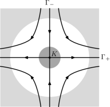
Figure 2. An illustration of Lemma 3.1, showing trajectories of $\varphi_{t}$ on $S^{*}M$. The shaded regions show places where $P_{\theta}-iQ-\omega^{2}$ is elliptic: the darker shaded region is $\{\sigma_{h}(Q)>0\}$ and the lighter shaded region is $\{f_{\theta}(r)\neq 0\}$.

Proof.

We follow [Dya15b, §4.3], see also [DZ, §6.2.1]. We use semiclassical elliptic and propagation estimates for solutions to the equation

$$\mathbf{P}u=f\in H^{s}(M),\quad u\in H^{s+2}(M)$$

where

$$\mathbf{P}:=P_{\theta}-iQ-\omega^{2}\in\Psi^{2}_{h}(M),\quad\sigma_{h}(\mathbf{P})=p_{\theta}-i\sigma_{h}(Q)-1.$$

The operator $\mathbf{P}$ is elliptic for $r\geq 2r_{1}$, since

$$\sigma_{h}(\mathbf{P})(y,\eta)={|\eta|^{2}\over(1+i\tan\theta)^{2}}-1\quad\text{for }|y|\geq 2r_{1}.$$

Moreover, $\mathbf{P}$ is elliptic near the fiber infinity of $M$, that is for large enough $|\xi|$. By the elliptic estimate in the class $\Psi^{2}_{h}(M)$ (see for instance [Zwo12, Theorem 4.29], [DZ16, Proposition 2.4], or [DZ, §E.2.2]) there exists $\chi\in C_{c}^{\infty}(M)$ such that for all $N$,

(3.9) $$\|(1-\chi)u\|_{H^{s+2}_{h}(M)}\leq C\|f\|_{H^{s}_{h}(M)}+\mathcal{O}(h^{\infty})\|u\|_{H^{-N}_{h}(M)}.$$

It remains to estimate $u$ in a compact set. By (3.3) and (3.4) the operator $\mathbf{P}$ is elliptic outside the set $S^{*}M\cap\{f_{\theta}(r)=0\}\cap\{\sigma_{h}(Q)=0\}$. By the elliptic estimate, we have for all $N$

(3.10) $$\begin{gathered}\|Bu\|_{H^{s+2}_{h}(M)}\leq C\|B^{\prime}f\|_{H^{s}_{h}(M)}+\mathcal{O}(h^{\infty})\|u\|_{H^{-N}_{h}(M)}\\ \text{for all compactly supported }B,B^{\prime}\in\Psi^{0}_{h}(M)\text{ such that}\\ \operatorname{WF}_{h}(B)\cap S^{*}M\cap\{f_{\theta}(r)=0\}\cap\{\sigma_{h}(Q)=0\}=\emptyset,\quad\operatorname{WF}_{h}(B)\subset\operatorname{ell}_{h}(B^{\prime}).\end{gathered}$$

To estimate $\|Au\|$ for general $A$, we use the following statement: for each $(x,\xi)\in T^{*}M$, there exists $T_{(x,\xi)}\geq 0$ such that

(3.11) $$\exp(-T_{(x,\xi)}H_{\mathop{\rm Re}\nolimits\sigma_{h}(\mathbf{P})})(x,\xi)\ \notin\ S^{*}M\cap\{f_{\theta}(r)=0\}\cap\{\sigma_{h}(Q)=0\}.$$

Indeed, assume the contrary, and put $\gamma(t)=\exp(tH_{\mathop{\rm Re}\nolimits\sigma_{h}(\mathbf{P})})(x,\xi)$. Clearly $(x,\xi)\in S^{*}M$. For all $t\leq 0$, we have $\gamma(t)\in\{f_{\theta}(r)=0\}$ and thus (using that $f_{\theta}^{\prime}(r)=f_{\theta}^{\prime\prime}(r)=0$ on $\{f_{\theta}(r)=0\}$)

$$\gamma(t)=\exp(tH_{p^{2}})(x,\xi)=\varphi_{2t}(x,\xi).$$

Now, if $(x,\xi)\in\Gamma_{+}$, then $\varphi_{-T}(x,\xi)\in\{\sigma_{h}(Q)>0\}$ for some $T>0$, by (2.8) and (3.5). If $(x,\xi)\notin\Gamma_{+}$, then $\varphi_{-T}(x,\xi)\in\{r\geq 2r_{1}\}\subset\{f_{\theta}(r)\neq 0\}$ for some $T>0$. In either case we reach a contradiction, finishing the proof of (3.11).

By (3.4) and (3.5),

(3.12) $$\mathop{\rm Im}\nolimits\sigma_{h}(\mathbf{P})\leq 0\quad\text{everywhere}.$$

Using semiclassical propagation of singularities (see for instance [DZ, Theorem E.49] or [DZ16, Proposition 2.5]) and (3.10), we deduce that

(3.13) $$\begin{gathered}\|Au\|_{H^{s+2}_{h}(M)}\leq Ch^{-1}\|A^{\prime}f\|_{H^{s}_{h}(M)}+\mathcal{O}(h^{\infty})\|u\|_{H^{-N}_{h}(M)}\\ \text{for all compactly supported }A,A^{\prime}\in\Psi^{0}_{h}(M)\text{ such that }\operatorname{WF}_{h}(A)\subset\operatorname{ell}_{h}(A^{\prime})\text{ and}\\ \varphi_{-2t}(x,\xi)\in\operatorname{ell}_{h}(A^{\prime})\text{ for all }(x,\xi)\in S^{*}M\cap\operatorname{WF}_{h}(A),\ t\in[0,T_{(x,\xi)}].\end{gathered}$$

Indeed, by a pseudodifferential partition of unity we may reduce to the case when $\operatorname{WF}_{h}(A)$ is contained in a small neighborhood of some $(x,\xi)\in\overline{T}^{*}M$. If $(x,\xi)\notin S^{*}M$, then we use (3.10). Otherwise we use propagation of singularities and (3.11), (3.12), and bound the term on the right-hand side of the propagation estimate by (3.10).

Together (3.9) and (3.13) imply that

(3.14) $$\|u\|_{H^{s+2}_{h}(M)}\leq Ch^{-1}\|\mathbf{P}u\|_{H^{s}_{h}(M)}+\mathcal{O}(h^{\infty})\|u\|_{H^{s+2}_{h}(M)}\quad\text{for all }u\in H^{s+2}(M).$$

As a compact perturbation of $P_{\theta}-\omega^{2}$, $\mathbf{P}$ is a Fredholm operator $H^{s+2}(M)\to H^{s}(M)$, therefore (3.14) implies that for $h$ small enough, $\mathbf{P}:H^{s+2}(M)\to H^{s}(M)$ is invertible and (3.7) holds. The restriction of the inverse to $C_{c}^{\infty}(M)$ does not depend on $s$.

It remains to show that under the condition (3.8), we have $A_{2}\mathcal{R}_{Q}(\omega)A_{1}=\mathcal{O}(h^{\infty})_{\Psi^{-\infty}(M)}$. If $\operatorname{WF}_{h}(A_{1})\cap S^{*}M=\emptyset$ or $\operatorname{WF}_{h}(A_{2})\cap S^{*}M=\emptyset$, this follows from the elliptic estimate; thus we may assume that $A_{1},A_{2}\in\Psi^{\operatorname*{comp}}_{h}(M)$. Take $\tilde{f}\in H^{-N}(M)$ and put

$$f:=A_{1}\tilde{f},\quad u:=\mathbf{P}^{-1}f.$$

By (3.8), we may find $A^{\prime}\in\Psi^{0}_{h}(M)$ such that $\operatorname{WF}_{h}(A_{1})\cap\operatorname{WF}_{h}(A^{\prime})=\emptyset$ and (3.13) holds for $A:=A_{2}$ and $A^{\prime}$. Then

$$\|A_{2}u\|_{H^{s+2}_{h}(M)}\leq Ch^{-1}\|A^{\prime}A_{1}\tilde{f}\|_{H^{s}_{h}(M)}+\mathcal{O}(h^{\infty})\|u\|_{H^{-N}_{h}(M)}=\mathcal{O}(h^{\infty})\|\tilde{f}\|_{H^{-N}_{h}(M)},$$

finishing the proof. ∎

We now prove two corollaries of Lemma 3.1, which in particular imply estimates on solutions to

(3.15) $$(P_{\theta}-\omega^{2})u=f,\quad u,f\in L^{2}(M),\quad\omega\in\widetilde{\Omega}.$$

The first statement implies that

$$\|A_{1}u\|_{H^{s+2}_{h}(M)}\leq Ch^{-1}\|f\|_{H^{s}_{h}(M)}+\mathcal{O}(h^{\infty})\|u\|_{H^{-N}_{h}(M)}\quad\text{when }\operatorname{WF}_{h}(A_{1})\cap\Gamma^{+}\cap S^{*}M=\emptyset.$$

Lemma 3.2.

Assume that $A_{1}\in\Psi^{0}_{h,\nu}(M)$ is compactly supported and $\operatorname{WF}_{h}(A_{1})\cap\Gamma^{+}\cap S^{*}M=\emptyset$. Then there exists a neighborhood $U$ of $K\cap S^{*}M$ such that for all $Q$ satisfying (3.5) and $\operatorname{WF}_{h}(Q)\subset U$, we have

(3.16) $$A_{1}\big{(}I-\mathcal{R}_{Q}(\omega)(P_{\theta}-\omega^{2})\big{)}=\mathcal{O}(h^{\infty})_{\Psi^{-\infty}},\quad\omega\in\widetilde{\Omega}.$$

Proof.

Choose $U$ such that

$$U\cap\operatorname{WF}_{h}(A_{1})=U\cap\bigcup_{t\geq 0}\varphi_{-t}\big{(}\operatorname{WF}_{h}(A_{1})\cap S^{*}M\big{)}=\emptyset.$$

This is possible by part 4 of Lemma 2.1. Now

$$A_{1}\big{(}I-\mathcal{R}_{Q}(\omega)(P_{\theta}-\omega^{2})\big{)}=-iA_{1}\mathcal{R}_{Q}(\omega)Q=\mathcal{O}(h^{\infty})_{\Psi^{-\infty}}$$

by the semiclassically outgoing property in Lemma 3.1 (inserting an operator in $\Psi_{h}^{0}(M)$ between $A_{1}$ and $\mathcal{R}_{Q}(\omega)$). ∎

The second corollary of Lemma 3.1 implies the following bound for solutions of (3.15):

$$\|u\|_{H^{s+2}_{h}}\leq C\|Bu\|_{H^{s}_{h}}+Ch^{-1}\|f\|_{H^{s}_{h}}+\mathcal{O}(h^{\infty})\|u\|_{H^{-N}_{h}}\quad\text{when }K\cap S^{*}M\subset\operatorname{ell}_{h}(B).$$

Lemma 3.3.

Assume that $B\in\Psi^{0}_{h}(M)$ is compactly supported and elliptic on $K\cap S^{*}M$. Then for all $Q$ satisfying (3.5) and $\operatorname{WF}_{h}(Q)\subset\operatorname{ell}_{h}(B)$, there exist $B_{0},B_{1},B_{2}\in\Psi^{\operatorname*{comp}}_{h}(M)$ such that

(3.17) $$I=(B_{1}+h\mathcal{R}_{Q}(\omega)B_{2})B+\mathcal{R}_{Q}(\omega)(I-B_{0})(P_{\theta}-\omega^{2})+\mathcal{O}(h^{\infty})_{\Psi^{-\infty}},\quad\omega\in\widetilde{\Omega}.$$

Proof.

Take $B_{0}$ such that

$$\operatorname{WF}_{h}(Q)\cap\operatorname{WF}_{h}(I-B_{0})=\emptyset,\quad\operatorname{WF}_{h}(B_{0})\subset\operatorname{ell}_{h}(B).$$

Then

$$I-B_{0}=\mathcal{R}_{Q}(\omega)(P_{\theta}-\omega^{2}-iQ)(I-B_{0})$$

implies that

$$I=B_{0}+\mathcal{R}_{Q}(\omega)(I-B_{0})(P_{\theta}-\omega^{2})-\mathcal{R}_{Q}(\omega)[P_{\theta},B_{0}]+\mathcal{O}(h^{\infty})_{\Psi^{-\infty}}.$$

It remains to use the elliptic parametrix construction to find $B_{1}$, $B_{2}$ so that

$$B_{2}B=-h^{-1}[P_{\theta},B_{0}]+\mathcal{O}(h^{\infty})_{\Psi^{-\infty}},\quad B_{1}B=B_{0}+\mathcal{O}(h^{\infty})_{\Psi^{-\infty}}$$

and (3.17) follows. ∎

The next statement, which is an important technical tool in the construction of the approximate inverse in §5.1, is obtained by iteration of Lemmas 2.4 and 3.2. See Figure 3.

Lemma 3.4.

Fix $\nu\in[0,1/2)$ and assume that a sequence of symbols

$$a_{j}\in S^{0}_{h,\nu}(T^{*}M),\quad j=0,1,\dots,L=L(h),\quad 0<L(h)\leq C\log(1/h)$$

is supported in a fixed compact subset $W\subset T^{*}M\setminus 0$ and each $S^{0}_{h,\nu}$ seminorm of $a_{j}$ is bounded uniformly in $j$. Assume moreover that $|a_{j}|\leq 1$ and there exists an $h$-independent open neighborhood $V$ of $\Gamma_{+}\cap S^{*}M$ and there exists $t_{1}>0$ bounded independently of $h$ such that the following dynamical conditions hold for all $j$:

(3.18) $$\varphi_{-t_{1}}(\operatorname*{supp}a_{j})\cap\operatorname*{supp}(1-a_{j+1})\cap V=\emptyset\quad\text{for all }j=0,\dots,L-1,$$

(3.19) $$\varphi_{-t}(W)\subset\{r<r_{1}\}\quad\text{for all }t\in[0,t_{1}].$$

Then we have for all $\omega\in\widetilde{\Omega}$, on $H^{2}(M)$

(3.20) $$\operatorname{Op}_{h}(a_{0})=Z(\omega)(P_{\theta}-\omega^{2})+J(\omega)\operatorname{Op}_{h}(a_{L})+\mathcal{O}(h^{\infty})_{\Psi^{-\infty}}$$

where $Z(\omega):L^{2}(M)\to H^{2}(M)$, $J(\omega):H^{-N}(M)\to H^{N}(M)$ are holomorphic in $\omega\in\widetilde{\Omega}$ and satisfy the bounds for each $\varepsilon_{1}>0$

(3.21) $$\|Z(\omega)\|_{H^{s}_{h}\to H^{s+2}_{h}} \leq C_{s,\varepsilon_{1}}h^{-1}\exp\big{(}(\tilde{\beta}t_{1}+\varepsilon_{1})L\big{)},$$

(3.22) $$\|J(\omega)\|_{H^{-N}_{h}\to H^{N}_{h}} \leq C_{N,\varepsilon_{1}}\exp\Big{(}\Big{(}-{\mathop{\rm Im}\nolimits\omega\over h}t_{1}+\varepsilon_{1}\Big{)}L\Big{)}.$$

Finally, if $a_{0}=1$ on some $h$-independent neighborhood of $K\cap S^{*}M$, then a decomposition of the form (3.20) holds with $\operatorname{Op}_{h}(a_{0})$ replaced by the identity operator.

Figure 3. An illustration of Lemma 3.4, showing the supports of $\psi a_{j}$, $(1-\psi)a_{j}$, and $(\psi a_{j})\circ\varphi_{t_{1}}$ (dashed), as well as $\varphi_{t_{1}}(V)$ (shaded). The arrows correspond to $\varphi_{t_{1}}$. At each step of the iteration, $(1-\psi)a_{j}$ is expressed using Lemma 3.2 and $\psi a_{j}$ is reduced to $a_{j+1}$ using Lemma 2.4.

Proof.

Fix $h$-independent $\psi\in C_{c}^{\infty}(\varphi_{t_{1}}(V);[0,1])$ such that

$$\operatorname*{supp}(1-\psi)\cap\Gamma_{+}\cap S^{*}M\cap W=\emptyset.$$

Then $\operatorname*{supp}((1-\psi)a_{j})$ is contained in an $h$-independent compact subset of $T^{*}M$ not intersecting $\Gamma_{+}\cap S^{*}M$, thus by Lemma 3.2 for an appropriate choice of $Q$ we have for $j=0,\dots,L-1$

(3.23) $$\operatorname{Op}_{h}\big{(}(1-\psi)a_{j}\big{)}=\operatorname{Op}_{h}\big{(}(1-\psi)a_{j}\big{)}\mathcal{R}_{Q}(\omega)(P_{\theta}-\omega^{2})+\mathcal{O}(h^{\infty})_{\Psi^{-\infty}}.$$

Next, by (3.18) we have

$$\varphi_{-t_{1}}(\operatorname*{supp}(\psi a_{j}))\cap\operatorname*{supp}(1-a_{j+1})=\emptyset.$$

Using (3.19), fix a multiplication operator $B^{\prime}=B^{\prime}(x)\in C_{c}^{\infty}(M;[0,1])$ such that

$$\operatorname*{supp}B^{\prime}\subset\{r<r_{1}\},\quad\operatorname*{supp}(1-B^{\prime})\cap\bigcup_{t=0}^{t_{1}}\varphi_{-t}(W)=\emptyset.$$

Since $P_{\theta}=-h^{2}\Delta_{g}$ on $\{r<r_{1}\}$, we have $B^{\prime}(P_{\theta}-\omega^{2})=B^{\prime}(-h^{2}\Delta_{g}-\omega^{2})$. Therefore by Lemma 2.4,

(3.24) $$\operatorname{Op}_{h}(\psi a_{j})=Z_{j}(\omega)B^{\prime}(P_{\theta}-\omega^{2})+e^{i\omega t_{1}/h}\operatorname{Op}_{h}(\psi a_{j})U(t_{1})\operatorname{Op}_{h}(a_{j+1})+\mathcal{O}(h^{\infty})_{\Psi^{-\infty}}$$

for all $\omega\in\widetilde{\Omega}$, where $Z_{j}(\omega)$ is holomorphic in $\omega\in\widetilde{\Omega}$ and satisfies

$$\|Z_{j}(\omega)\|_{H^{-N}_{h}\to H^{N}_{h}}\leq C_{N}h^{-1}$$

and the constant $C_{N}$, as well as the constants in $\mathcal{O}(h^{\infty})_{\Psi^{-\infty}}$, is independent of $h$ and $j$.

Adding (3.23) and (3.24) and iterating in $j$, we obtain (3.20) with

$$Z(\omega) =\sum_{j=0}^{L-1}e^{i\omega jt_{1}/h}\Big{(}\prod_{\ell=0}^{j-1}\operatorname{Op}_{h}(\psi a_{\ell})U(t_{1})\Big{)}\big{(}\operatorname{Op}_{h}\big{(}(1-\psi)a_{j}\big{)}\mathcal{R}_{Q}(\omega)+Z_{j}(\omega)B^{\prime}\big{)},$$

$$J(\omega) =e^{i\omega Lt_{1}/h}\prod_{j=0}^{L-1}\operatorname{Op}_{h}(\psi a_{j})U(t_{1}).$$

The bounds (3.21) and (3.22) follow from here and estimate on the operator norm following from (2.20):

$$\max_{j}\|\operatorname{Op}_{h}(\psi a_{j})\|_{L^{2}\to L^{2}}\leq 1+o(1)\quad\text{as }h\to 0.$$

In particular, for any fixed $\varepsilon_{1}>0$ we have

$$\max_{0\leq j\leq L}\Big{\|}\prod_{\ell=0}^{j-1}\operatorname{Op}_{h}(\psi a_{\ell})U(t_{1})\Big{\|}_{H^{-N}_{h}\to H^{N}_{h}}\leq C_{N}e^{\varepsilon_{1}L}.$$

To show the last statement of the lemma, assume that $a_{0}=1$ on an $h$-independent neighborhood $\mathcal{U}$ of $K\cap S^{*}M$. Take $B\in\Psi^{\operatorname*{comp}}_{h}(M)$ elliptic on $K\cap S^{*}M$ and satisfying $\operatorname{WF}_{h}(B)\subset\mathcal{U}$. Then by Lemma 3.3, we have for an appropriate choice of $Q,B_{0},B_{1},B_{2}\in\Psi^{\operatorname*{comp}}_{h}(M)$,

$$I=\mathcal{R}_{Q}(\omega)(I-B_{0})(P_{\theta}-\omega^{2})+(B_{1}+h\mathcal{R}_{Q}(\omega)B_{2})B\operatorname{Op}_{h}(a_{0})+\mathcal{O}(h^{\infty})_{\Psi^{-\infty}}.$$

Combining this with the representation (3.20) of $\operatorname{Op}_{h}(a_{0})$, we obtain (3.20) with the identity operator on the left-hand side. ∎

3.2. Wave propagator

We next study the long time behavior of the half-wave propagator $U(t)=\exp(-it\sqrt{-\Delta_{g}})$. We first prove a microlocal estimate on the free half-wave propagator on $\mathbb{R}^{d}$,

$$U_{0}(t)=\exp(-it\sqrt{-\Delta_{0}}):\ L^{2}(\mathbb{R}^{d})\to L^{2}(\mathbb{R}^{d}),$$

where $\Delta_{0}$ is the flat Laplacian.

Lemma 3.5.

Let $A_{1},A_{2}\in\Psi^{k}_{h}(\mathbb{R}^{d})$ such that there exists $R>0$ with

$$\operatorname{WF}_{h}(A_{1})\cup\operatorname{WF}_{h}(A_{2})\ \subset\ \{|y|<R\},$$

at least one of $\operatorname{WF}_{h}(A_{1})$, $\operatorname{WF}_{h}(A_{2})$ is a compact subset of $T^{*}\mathbb{R}^{d}\setminus 0$, and

(3.25) $$(y^{\prime},\eta)\in\operatorname{WF}_{h}(A_{1}),\ \eta\neq 0,\ t\geq 0\ \Longrightarrow\ \Big{(}y^{\prime}+t{\eta\over|\eta|},\eta\Big{)}\notin\operatorname{WF}_{h}(A_{2}).$$

Then we have the following version of propagation of singularities which is uniform in $t\geq 0$:

(3.26) $$A_{2}U_{0}(t)A_{1}=\mathcal{O}(h^{\infty})_{\Psi^{-\infty}(\mathbb{R}^{d})}.$$

Proof.

Write $A_{1}=\operatorname{Op}_{h}(a_{1})^{*}+\mathcal{O}(h^{\infty})_{\Psi^{-\infty}}$, $A_{2}=\operatorname{Op}_{h}(a_{2})+\mathcal{O}(h^{\infty})_{\Psi^{-\infty}}$ for some $a_{1},a_{2}$ whose supports satisfy the conditions imposed on $\operatorname{WF}_{h}(A_{1})$, $\operatorname{WF}_{h}(A_{2})$, including (3.25). The Schwartz kernel of $\operatorname{Op}_{h}(a_{2})U_{0}(t)\operatorname{Op}_{h}(a_{1})^{*}$ is compactly supported and given by

(3.27) $$\mathcal{K}(y,y^{\prime})=(2\pi h)^{-2d}\int_{\mathbb{R}^{d}}e^{\frac{i}{h}(\langle y-y^{\prime},\eta\rangle-t|\eta|)}a_{2}(y,\eta)\overline{a_{1}(y^{\prime},\eta)}\,d\eta.$$

Put $\Phi=\langle y-y^{\prime},\eta\rangle-t|\eta|$. Then there exists $c>0$ such that on the support of $a_{2}(y,\eta)\overline{a_{1}(y^{\prime},\eta)}$,

(3.28) $$|\partial_{\eta}\Phi|=\Big{|}y-y^{\prime}-t\frac{\eta}{|\eta|}\Big{|}\geq c\langle t\rangle>0.$$

Indeed, since $y,y^{\prime}$ vary in a compact set and $\eta$ is bounded away from zero, it is enough to consider the case of bounded $t$. Then (3.28) follows from (3.25).

Now, repeated integration by parts in $\eta$ gives that for each $N$,

$$\|\mathcal{K}\|_{C^{N}(\mathbb{R}^{2d})}\ \leq\ C_{N}h^{N}\langle t\rangle^{-N}.$$

This completes the proof. ∎

We next use $U_{0}(t)$ to write a parametrix for the propagator $U(t)$. For $\psi_{0}\in C_{c}^{\infty}(M)$ with $\operatorname*{supp}(1-\psi_{0})\subset\{r>r_{0}\}$ and $u\in L^{2}(M)$, we define

$$(1-\psi_{0})U_{0}(t)(1-\psi_{0})u\in L^{2}(M)$$

as follows: we pull back the restriction of $(1-\psi_{0})u$ to each infinite end to $\mathbb{R}^{d}$ using the Euclidean coordinate, apply $(1-\psi_{0})U_{0}(t)$, and take the sum of the resulting functions pulled back to $M$. This gives an operator

(3.29) $$(1-\psi_{0})U_{0}(t)(1-\psi_{0}):L^{2}(M)\to L^{2}(M).$$

Recall the sets $\mathcal{E}_{\pm},\mathcal{E}_{\pm}^{\circ}$ defined in (2.3).

Lemma 3.6.

Suppose that $A_{\pm}\in\Psi^{\operatorname*{comp}}_{h}(M)$, $\psi_{0}\in C_{c}^{\infty}(M)$ satisfy for some $r_{2}>r_{0}$ (see Figure 4)

$$\operatorname{WF}_{h}(A_{\pm})\subset\mathcal{E}_{\pm}^{\circ}\cap\{r>r_{2}\},\quad\operatorname*{supp}\psi_{0}\subset\{r<r_{2}\},\quad\operatorname*{supp}(1-\psi_{0})\subset\{r>r_{0}\}.$$

Then we have uniformly in $0\leq t\leq Ch^{-1}$

(3.30) $$U(t)A_{+}=(1-\psi_{0})U_{0}(t)(1-\psi_{0})A_{+}+\mathcal{O}(h^{\infty})_{\Psi^{-\infty}}$$

(3.31) $$U(-t)A_{-}=(1-\psi_{0})U_{0}(-t)(1-\psi_{0})A_{-}+\mathcal{O}(h^{\infty})_{\Psi^{-\infty}}.$$

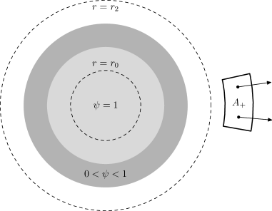
Figure 4. An illustration of Lemma 3.6 when $0\leq\psi_{0}\leq 1$, showing the regions $\psi_{0}=1$ and $0<\psi_{0}<1$ (shaded) and the projection of $\operatorname{WF}_{h}(A_{+})$ onto $M$. The points $(x,\xi)$ in $\operatorname{WF}_{h}(A)$, pictured by arrows, give rise to trajectories escaping to infinity in the future and never entering $\operatorname*{supp}\psi_{0}$.

Proof.

We prove (3.30), with (3.31) established similarly. For simplicity of notation, we present the argument in the case when $M$ is diffeomorphic to $\mathbb{R}^{d}$. The general case is proved in the same way, reducing to the case when $A_{+}$ is supported on one infinite end and treating $1-\psi_{0}$ on this infinite end as an operator $L^{2}(M)\to L^{2}(\mathbb{R}^{d})$ and $L^{2}(\mathbb{R}^{d})\to L^{2}(M)$. We identify $M$ with $\mathbb{R}^{d}$ and use the quantization (2.15).

Since $U_{0}(t),U(t)$ are bounded uniformly in $t$ on all Sobolev spaces and $\operatorname{WF}_{h}(A_{+})\cap\operatorname*{supp}\psi_{0}=\emptyset$,

$$U(t)A_{+} =U(t)(1-\psi_{0})^{2}A_{+}+\mathcal{O}(h^{\infty})_{\Psi^{-\infty}}.$$

Therefore it remains to show that uniformly in $0\leq t\leq Ch^{-1}$,

(3.32) $$W(t)=\mathcal{O}(h^{\infty})_{\Psi^{-\infty}},$$

where the operator $W(t)$ on $L^{2}(M)$ is defined by

$$W(t):=\big{(}(1-\psi_{0})U_{0}(t)-U(t)(1-\psi_{0})\big{)}(1-\psi_{0})A_{+}.$$

Using the wave operator $\Box_{g}=\partial_{t}^{2}-\Delta_{g}$, we write

(3.33) $$W(t)=\cos(t\sqrt{-\Delta_{g}})W(0)+{\sin(t\sqrt{-\Delta_{g}})\over\sqrt{-\Delta_{g}}}W^{\prime}(0)+\int_{0}^{t}{\sin\big{(}(t-t^{\prime})\sqrt{-\Delta_{g}}\big{)}\over\sqrt{-\Delta_{g}}}\Box_{g}W(t^{\prime})\,dt^{\prime}.$$

We compute

(3.34) $$W(0)=0.$$

Next,

(3.35) $$ihW^{\prime}(0)=\big{(}(1-\psi_{0})h\sqrt{-\Delta_{0}}-h\sqrt{-\Delta_{g}}(1-\psi_{0})\big{)}(1-\psi_{0})A_{+}=\mathcal{O}(h^{\infty})_{\Psi^{-\infty}}.$$

Indeed, by (2.24) both $(1-\psi_{0})h\sqrt{-\Delta_{0}}(1-\psi_{0})A_{+}$ and $h\sqrt{-\Delta_{g}}(1-\psi_{0})^{2}A_{+}$ are in $\Psi^{0}_{h}(M)$. As explained in the discussion following [DS99, Theorem 8.7], the asymptotic expansion for the full symbol of each of these operators at some point can be computed using only the derivatives of $\psi_{0}$ and the full symbols of $A_{+},\Delta_{0},\Delta_{g}$ at this point. Since $\Delta_{0}=\Delta_{g}$ and $\psi_{0}=0$ on $\{r>r_{2}\}\supset\operatorname{WF}_{h}(A_{+})$, we obtain (3.35).

Finally, since $\Delta_{0}=\Delta_{g}$ on $\{r>r_{0}\}\supset\operatorname*{supp}(1-\psi_{0})$, we have

$$h^{2}\Box_{g}W(t)=[h^{2}\Delta_{g},\psi_{0}]U_{0}(t)(1-\psi_{0})A_{+}.$$

Now, with $A_{2}:=[h^{2}\Delta_{g},\psi_{0}]$

$$\operatorname{WF}_{h}(A_{2})\ \subset\ \operatorname*{supp}d\psi_{0}\ \subset\ \{r_{0}<r<r_{2}\}.$$

Then $A_{2}$ and $A_{1}:=A_{+}$ satisfy (3.25), thus by Lemma 3.5

(3.36) $$h^{2}\Box_{g}W(t)=\mathcal{O}(h^{\infty})_{\Psi^{-\infty}}.$$

Now (3.32) follows from (3.33)–(3.36), the bound $t\leq Ch^{-1}$, and the fact that for each $s$, the operators

$$\cos(t\sqrt{-\Delta_{g}}),{\sin(t\sqrt{-\Delta_{g}})\over\sqrt{-\Delta_{g}}}:H^{s}_{h}(M)\to H^{s}_{h}(M)$$

are bounded in norm by $C\langle t\rangle$. ∎

The next lemma shows that for times $t=\mathcal{O}(\log(1/h))$, the cutoff wave propagator $A_{2}U(t)A_{1}$, where $A_{j}\in\Psi^{\operatorname*{comp}}_{h,\nu}(T^{*}M)$ and $\operatorname{WF}_{h}(A_{j})$ lies near $S^{*}M$, can be expressed in terms of cutoff wave propagators for bounded time. It relies on Lemmas 3.5 and 3.6 and is a key component of the proof of Lemma 6.1 below.

Lemma 3.7.

Let $A_{1}\in\Psi^{\operatorname*{comp}}_{h,\nu}(M)$, $A_{2}\in\Psi^{0}_{h,\nu}(M)$, and $\chi\in S^{0}_{h}(T^{*}M;[0,1])$ satisfy for some $\varepsilon_{E}>0$ and $r_{2}>r_{0}$

(3.37) $$\operatorname{WF}_{h}(A_{1})\cup\operatorname{WF}_{h}(A_{2})\cup\operatorname*{supp}\chi\subset\{r<r_{2}\},\quad\operatorname{WF}_{h}(A_{1})\subset\{|\xi|_{g}^{2}\in(1-\varepsilon_{E},1+\varepsilon_{E})\},$$

(3.38) $$\operatorname*{supp}(1-\chi)\cap\{|\xi|_{g}^{2}\in[1-\varepsilon_{E},1+\varepsilon_{E}]\}\cap\{r\leq r_{0}\}=\emptyset.$$

Put $T:=\sqrt{r_{2}^{2}-r_{0}^{2}}$ and let $C$ be an $h$-independent constant. Then for each sequence of times

$$t_{1},\dots,t_{L}\geq T,\quad L\leq Ch^{-1},\quad t_{j}\leq C,$$

we have

$$A_{2}U(t_{1}+\dots+t_{L})A_{1}=A_{2}U(t_{1})\operatorname{Op}_{h}(\chi)U(t_{2})\cdots\operatorname{Op}_{h}(\chi)U(t_{L})A_{1}+\mathcal{O}(h^{\infty})_{\Psi^{-\infty}}.$$

Proof.

We may assume that $A_{1}\in\Psi^{\operatorname*{comp}}_{h}(M)$, $A_{2}\in\Psi^{0}_{h}(M)$. Indeed, otherwise we may take $A^{\prime}_{1}\in\Psi^{\operatorname*{comp}}_{h}(M)$, $A^{\prime}_{2}\in\Psi^{0}_{h}(M)$ such that $(I-A^{\prime}_{1})A_{1}=\mathcal{O}(h^{\infty})_{\Psi^{-\infty}}$, $A_{2}(I-A^{\prime}_{2})=\mathcal{O}(h^{\infty})_{\Psi^{-\infty}}$, and $\operatorname{WF}_{h}(A^{\prime}_{1})$, $\operatorname{WF}_{h}(A^{\prime}_{2})$ satisfy (3.37), and apply the argument below with $A_{1},A_{2}$ replaced by $A^{\prime}_{1},A^{\prime}_{2}$.

We have

$$\begin{gathered}A_{2}U(t_{1}+\dots+t_{L})A_{1}-A_{2}U(t_{1})\operatorname{Op}_{h}(\chi)U(t_{2})\cdots\operatorname{Op}_{h}(\chi)U(t_{L})A_{1}=\sum_{\ell=1}^{L-1}B_{\ell},\\ B_{\ell}:=A_{2}U(t_{1})\operatorname{Op}_{h}(\chi)\cdots U(t_{\ell-1})\operatorname{Op}_{h}(\chi)U(t_{\ell})\operatorname{Op}_{h}(1-\chi)U(t_{\ell+1}+\dots+t_{L})A_{1}.\end{gathered}$$

Therefore it suffices to show that $B_{\ell}=\mathcal{O}(h^{\infty})_{L^{2}\to L^{2}}$ uniformly in $\ell$. Since $U(t)$ is unitary and $\operatorname{Op}_{h}(\chi)$ satisfies the norm bound [Zwo12, Theorem 13.13]

(3.39) $$\|\operatorname{Op}_{h}(\chi)\|_{H^{s}_{h}\to H^{s}_{h}}\leq 1+\mathcal{O}(h),$$

it is enough to show the following bounds uniform in $\ell$ (in fact (3.40) is used only for $\ell=2,\dots,L-1$ and (3.41) is used only for $\ell=1$)

(3.40) $$\operatorname{Op}_{h}(\chi)U(t_{\ell})\operatorname{Op}_{h}(1-\chi)U(t_{\ell+1}+\dots+t_{L})A_{1}=\mathcal{O}(h^{\infty})_{\Psi^{-\infty}},$$

(3.41) $$A_{2}U(t_{\ell})\operatorname{Op}_{h}(1-\chi)U(t_{\ell+1}+\dots+t_{L})A_{1}=\mathcal{O}(h^{\infty})_{\Psi^{-\infty}}.$$

We show (3.40) with the same proof giving (3.41) as well. Take $\psi_{1}\in C_{c}^{\infty}(\mathbb{R})$ such that

$$\operatorname*{supp}\psi_{1}\subset(1-\varepsilon_{E},1+\varepsilon_{E}),\quad\operatorname{WF}_{h}(A_{1})\cap\operatorname*{supp}\big{(}1-\psi_{1}(|\xi|_{g}^{2})\big{)}=\emptyset.$$

We can replace $A_{1}$ by $\psi_{1}(-h^{2}\Delta_{g})A_{1}$ in (3.40) since

$$(I-\psi_{1}(-h^{2}\Delta_{g}))A_{1}=\mathcal{O}(h^{\infty})_{\Psi^{-\infty}}.$$

Since $U(t_{\ell+2}+\dots+t_{L})$ commutes with $\psi_{1}(-h^{2}\Delta_{g})$, it suffices to show that

(3.42) $$AU(t_{\ell+2}+\dots+t_{L})A_{1}=\mathcal{O}(h^{\infty})_{\Psi^{-\infty}},$$

where

$$A:=U(-t_{\ell}-t_{\ell+1})\operatorname{Op}_{h}(\chi)U(t_{\ell})\operatorname{Op}_{h}(1-\chi)U(t_{\ell+1})\psi_{1}(-h^{2}\Delta_{g}).$$

By Lemma 2.3, we have $A\in\Psi^{\operatorname*{comp}}_{h}(M)$ and

$$\operatorname{WF}_{h}(A)\subset\varphi_{-t_{\ell}-t_{\ell+1}}(\operatorname*{supp}\chi)\cap\varphi_{-t_{\ell+1}}(\operatorname*{supp}(1-\chi))\cap\{|\xi|^{2}_{g}\in(1-\varepsilon_{E},1+\varepsilon_{E})\}.$$

Take $\mathbf{x}\in\varphi_{t_{\ell+1}}(\operatorname{WF}_{h}(A))$. By (3.38) we have $\mathbf{x}\in\{r>r_{0}\}$ and by (3.37) we have $\varphi_{t_{\ell}}(\mathbf{x})\in\{r<r_{2}\}$. By (2.4) and since $t_{\ell}\geq T$ we see that $\mathbf{x}\in\mathcal{E}_{-}^{\circ}$. Applying (2.4) again and using that $t_{\ell+1}\geq T$ we see that $\varphi_{-t_{\ell+1}-s}(\mathbf{x})\in\mathcal{E}_{-}^{\circ}\cap\{r>r_{2}\}$ for all $s\geq 0$. Therefore

(3.43) $$\operatorname{WF}_{h}(A)\subset\mathcal{E}_{-}^{\circ}\cap\{r>r_{2}\},$$

(3.44) $$\varphi_{-s}(\operatorname{WF}_{h}(A))\cap\operatorname{WF}_{h}(A_{1})=\emptyset\quad\text{for all }s\geq 0.$$

Denote $\tilde{t}_{\ell}:=t_{\ell+2}+\dots+t_{L}\in[0,Ch^{-1}]$. By (3.43) we may apply Lemma 3.6 to get for some $\psi_{0}\in C_{c}^{\infty}(M;\mathbb{R})$, $\operatorname*{supp}(1-\psi_{0})\subset\{r>r_{0}\}$

$$U(-\tilde{t}_{\ell})A^{*}=(1-\psi_{0})U_{0}(-\tilde{t}_{\ell})(1-\psi_{0})A^{*}+\mathcal{O}(h^{\infty})_{\Psi^{-\infty}}.$$

Taking adjoints, we get

(3.45) $$AU(\tilde{t}_{\ell})=A(1-\psi_{0})U_{0}(\tilde{t}_{\ell})(1-\psi_{0})+\mathcal{O}(h^{\infty})_{\Psi^{-\infty}}.$$

By Lemma 3.5 and (3.44) we have

(3.46) $$A(1-\psi_{0})U_{0}(\tilde{t}_{\ell})(1-\psi_{0})A_{1}=\mathcal{O}(h^{\infty})_{\Psi^{-\infty}}.$$

Combining (3.45) and (3.46), we obtain (3.42), finishing the proof. ∎

Using Lemma 3.7, we also obtain the following estimate used in §6.3:

Lemma 3.8.

Assume that $A_{1}\in\Psi^{\operatorname*{comp}}_{h}(M),A_{2}\in\Psi^{0}_{h}(M)$ satisfy for some $r_{1}>r_{0}$ and $\varepsilon_{E}>0$

(3.47) $$\operatorname{WF}_{h}(A_{1})\subset\{r<r_{1}\}\cap\{|\xi|_{g}^{2}\in(1-\varepsilon_{E},1+\varepsilon_{E})\},\quad\operatorname{WF}_{h}(A_{2})\subset\{r<r_{1}\}.$$

Put $T_{0}:=\sqrt{r_{1}^{2}-r_{0}^{2}}$ and assume that $\chi^{\prime}\in C_{c}^{\infty}(M)$ satisfies

(3.48) $$\operatorname*{supp}(1-\chi^{\prime})\cap\{r\leq r_{1}+T_{0}\}=\emptyset.$$

Fix $C_{0}>0$. Then for all $t\in[T_{0},C_{0}h^{-1}]$, $s\in[0,C_{0}h^{-1}]$, and $u\in L^{2}(M)$ we have

$$\|A_{2}U(s+t)A_{1}u\|_{L^{2}}\leq\|A_{2}\|_{L^{2}\to L^{2}}\cdot\|\chi^{\prime}U(t)A_{1}u\|_{L^{2}}+\mathcal{O}(h^{\infty})\|u\|_{L^{2}}.$$

Proof.

We first consider the case $s\geq T_{0}$. Fix $\chi\in C_{c}^{\infty}(M;[0,1])$ such that

$$\operatorname*{supp}\chi\subset\{r<r_{1}\},\quad\operatorname*{supp}(1-\chi)\cap\{r\leq r_{0}\}=\emptyset.$$

We write

$$t=t_{1}+\dots+t_{L},\quad s=s_{1}+\dots+s_{L^{\prime}},\quad t_{j},s_{j}\in[T_{0},2T_{0}],\quad L,L^{\prime}\leq C_{0}h^{-1}.$$

By Lemma 3.7 (with $(r_{1},T_{0})$ taking the place of $(r_{2},T)$) we have

$$A_{2}U(s+t)A_{1}=A_{2}U(s_{1})\chi\cdots U(s_{L^{\prime}})\chi U(t_{1})\cdots\chi U(t_{L})A_{1}+\mathcal{O}(h^{\infty})_{\Psi^{-\infty}}.$$

Therefore

$$\|A_{2}U(s+t)A_{1}u\|_{L^{2}}\leq\|A_{2}\|_{L^{2}\to L^{2}}\cdot\|\chi U(t_{1})\cdots\chi U(t_{L})A_{1}u\|_{L^{2}}+\mathcal{O}(h^{\infty})\|u\|_{L^{2}}.$$

Another application of Lemma 3.7 gives

$$\|\chi U(t_{1})\cdots\chi U(t_{L})A_{1}u-\chi U(t)A_{1}u\|_{L^{2}}=\mathcal{O}(h^{\infty})\|u\|_{L^{2}},$$

finishing the proof since $\chi=\chi\chi^{\prime}$.

We now consider the case $0\leq s\leq T_{0}$. Fix $\psi_{1}\in C_{c}^{\infty}(\mathbb{R};[0,1])$ such that $\operatorname*{supp}\psi_{1}\subset(0,\infty)$ and $\operatorname*{supp}(1-\psi_{1})\cap[1-\varepsilon_{E},1+\varepsilon_{E}]=\emptyset$. Since $U(t)$ commutes with $\psi_{1}(-h^{2}\Delta_{g})$, we have

$$A_{2}U(s+t)A_{1} =A_{2}U(s+t)\psi_{1}(-h^{2}\Delta_{g})A_{1}+\mathcal{O}(h^{\infty})_{\Psi^{-\infty}}$$

$$=A_{2}U(s)\psi_{1}(-h^{2}\Delta_{g})U(t)A_{1}+\mathcal{O}(h^{\infty})_{\Psi^{-\infty}}.$$

Therefore

$$\|A_{2}U(s+t)A_{1}u\|_{L^{2}}\leq\|U(-s)A_{2}U(s)\psi_{1}(-h^{2}\Delta_{g})U(t)A_{1}u\|_{L^{2}}+\mathcal{O}(h^{\infty})\|u\|_{L^{2}}.$$

By (3.47) and (3.48) we have $(T^{*}M\setminus 0)\cap\varphi_{-s}(\operatorname{WF}_{h}(A_{2}))\cap\operatorname*{supp}(1-\chi^{\prime})=\emptyset$. Therefore by Lemma 2.3

$$U(-s)A_{2}U(s)\psi_{1}(-h^{2}\Delta_{g})(1-\chi^{\prime})=\mathcal{O}(h^{\infty})_{\Psi^{-\infty}}.$$

Therefore

$$\|U(-s)A_{2}U(s)\psi_{1}(-h^{2}\Delta_{g})U(t)A_{1}u\|_{L^{2}}\leq\|A_{2}\|_{L^{2}\to L^{2}}\cdot\|\chi^{\prime}U(t)A_{1}u\|_{L^{2}}+\mathcal{O}(h^{\infty})\|u\|_{L^{2}}$$

finishing the proof. ∎

4. Dynamical cutoff functions

In this section, we construct families of auxiliary cutoff functions which localize to smaller and smaller neighborhoods of $\Gamma_{\pm}$ and are the key component of the proofs of Theorems 2 and 3. These functions are defined by propagating a fixed cutoff function for a large time.

Fix constants

$$0\leq\rho<2\nu<1.$$

We propagate up to time $\rho t_{e}$ where $t_{e}$ is the Ehrenfest time from (1.7) in the semiclassical scaling:

(4.1) $$t_{e}={\log(1/h)\over 2\Lambda_{\max}}.$$

Fix a cutoff function

(4.2) $$\chi\in C_{c}^{\infty}(T^{*}M\setminus 0;[0,1]),\quad\operatorname*{supp}(1-\chi)\cap K\cap S^{*}M=\emptyset.$$

Define the following functions living near $\Gamma_{\pm}$:

(4.3) $$\chi_{t}^{+}=\chi(\chi\circ\varphi_{-t}),\quad\chi_{t}^{-}=\chi(\chi\circ\varphi_{t}),\quad t\geq 0.$$

By the derivative estimates for the flow $\varphi_{t}$ (see for instance [DG16, Lemma C.1]) we have uniformly in $t$,

(4.4) $$\chi_{t}^{\pm}\in S^{\operatorname*{comp}}_{h,\nu}(T^{*}M),\quad 0\leq t\leq\rho t_{e}.$$

By (2.9), there exists $T>0$ such that

(4.5) $$\varphi_{t_{1}}(\operatorname*{supp}\chi)\cap\varphi_{-t_{2}}(\operatorname*{supp}\chi)\cap\operatorname*{supp}(1-\chi)\cap S^{*}M=\emptyset\quad\text{for all }t_{1},t_{2}\geq T.$$

This implies the following

Lemma 4.1.

Let $\chi,T$ satisfy (4.2), (4.5). Then for all $t_{0}\geq T,t\geq 0$,

(4.6) $$\varphi_{t_{0}+T}(\operatorname*{supp}\chi^{+}_{t})\cap\operatorname*{supp}(\chi-\chi^{+}_{t+t_{0}})\cap S^{*}M =\emptyset,$$

(4.7) $$\varphi_{-t_{0}-T}(\operatorname*{supp}\chi^{-}_{t})\cap\operatorname*{supp}(\chi-\chi^{-}_{t+t_{0}})\cap S^{*}M =\emptyset,$$

(4.8) $$\varphi_{-t_{0}}(\operatorname*{supp}\chi)\cap\operatorname*{supp}(1-\chi)\cap\Gamma_{+}\cap S^{*}M =\emptyset,$$

(4.9) $$\varphi_{t_{0}}(\operatorname*{supp}\chi)\cap\operatorname*{supp}(1-\chi)\cap\Gamma_{-}\cap S^{*}M =\emptyset.$$

Proof.

For (4.6) it is enough to show that

$$\varphi_{t+t_{0}+T}(\operatorname*{supp}\chi)\cap\operatorname*{supp}\chi\cap\varphi_{t+t_{0}}(\operatorname*{supp}(1-\chi))\cap S^{*}M=\emptyset$$

which follows immediately by applying $\varphi_{t+t_{0}}$ to (4.5) with $t_{1}=T,t_{2}=t+t_{0}$.

For (4.7) it is enough to show that

$$\varphi_{-t-t_{0}-T}(\operatorname*{supp}\chi)\cap\operatorname*{supp}\chi\cap\varphi_{-t-t_{0}}(\operatorname*{supp}(1-\chi))\cap S^{*}M=\emptyset$$

which follows immediately by applying $\varphi_{-t-t_{0}}$ to (4.5) with $t_{1}=t+t_{0},t_{2}=T$.

To show (4.8), choose $(x,\xi)$ in the left-hand side of this equation. Since $(x,\xi)\in\Gamma_{+}$, by (2.8) we have $(x,\xi)\in\varphi_{t_{1}}(\operatorname*{supp}\chi)$ for all $t_{1}\geq 0$ large enough depending on $(x,\xi)$. Then

$$(x,\xi)\in\varphi_{-t_{0}}(\operatorname*{supp}\chi)\cap\varphi_{t_{1}}(\operatorname*{supp}\chi)\cap\operatorname*{supp}(1-\chi)\cap S^{*}M$$

which is impossible by (4.5) with $t_{2}=t_{0}$, as soon as $t_{1}\geq T$.

Finally, to show (4.9), choose $(x,\xi)$ in the left-hand side of this equation. Since $(x,\xi)\in\Gamma_{-}$, by (2.8) we have $(x,\xi)\in\varphi_{-t_{2}}(\operatorname*{supp}\chi)$ for all $t_{2}\geq 0$ large enough depending on $(x,\xi)$. Then

$$(x,\xi)\in\varphi_{t_{0}}(\operatorname*{supp}\chi)\cap\varphi_{-t_{2}}(\operatorname*{supp}\chi)\cap\operatorname*{supp}(1-\chi)\cap S^{*}M$$

which is impossible by (4.5) with $t_{1}=t_{0}$ as soon as $t_{2}\geq T$. ∎

5. Proof of the Weyl upper bound

In this section, we prove Theorem 2, following the method of [Dya15a]. We use the function $\chi$ and the constant $T$ satisfying (4.2), (4.5). We also assume that $\chi$ is chosen to be homogeneous of degree 0 near $S^{*}M$ and $\operatorname*{supp}\chi\subset\{r<r_{0}\}\cap\{|\xi|_{g}\leq 2\}$. We fix $h$-dependent

(5.1) $$\rho,\rho^{\prime}\in[0,1),\quad{1\over 2}\max(\rho,\rho^{\prime})<\nu<{1\over 2},\quad\rho t_{e},\rho^{\prime}t_{e}\geq C_{0},$$

with $C_{0}$ a large constant, $\rho,\rho^{\prime}$ chosen at the end of the proof, and $\nu$ independent of $h$, and define the following functions using (4.1) and (4.3):

$$\chi_{+}:=\chi^{+}_{\rho t_{e}},\quad\chi_{-}:=\chi^{-}_{\rho^{\prime}t_{e}},$$

which both lie in $S^{\operatorname*{comp}}_{h,\nu}(T^{*}M)$ by (4.4). We also use a function

(5.2) $$\chi_{E}\in\mathscr{S}(\mathbb{R}),\quad\chi_{E}(0)=1,\quad\operatorname*{supp}\widehat{\chi}_{E}\subset(-1,1).$$

5.1. Approximate inverse

We first construct an approximate inverse for the complex scaled operator $P_{\theta}-\omega^{2}$ (see §3.1), arguing similarly to the proof of [Dya15a, Proposition 2.1] and using the results of §4. See (3.2) for the definitions of $\widetilde{\Omega},\tilde{\beta}$.

Lemma 5.1.

Fix $\varepsilon_{0}>0$. Then there exist $h$-dependent families of operators holomorphic in $\omega\in\widetilde{\Omega}$

(5.3) $$\mathcal{Z}(\omega):L^{2}(M)\to H^{2}(M), \qquad\|\mathcal{Z}(\omega)\|_{L^{2}(M)\to H^{2}_{h}(M)}\leq Ch^{-1}e^{(\tilde{\beta}+\varepsilon_{0})(\rho+\rho^{\prime})t_{e}},$$

(5.4) $$\mathcal{J}(\omega):H^{2}(M)\to H^{2}(M), \qquad\|\mathcal{J}(\omega)\|_{H^{2}_{h}(M)\to H^{2}_{h}(M)}\leq Ce^{(-h^{-1}\mathop{\rm Im}\nolimits\omega+\varepsilon_{0})\rho^{\prime}t_{e}},$$

such that for all $\omega\in\widetilde{\Omega}$ and the constant $C_{0}$ in (5.1) chosen large enough, we have on $H^{2}(M)$

(5.5) $$I=\mathcal{Z}(\omega)(P_{\theta}-\omega^{2})+\mathcal{J}(\omega)\operatorname{Op}_{h}(\chi_{-})\operatorname{Op}_{h}(\chi_{+})\chi_{E}\Big{(}{-h^{2}\Delta_{g}-\omega^{2}\over h}\Big{)}+\mathcal{R}(\omega),$$

and the remainder $\mathcal{R}(\omega)$ is $\mathcal{O}(h^{\infty})_{\Psi^{-\infty}}$.

Proof.

Throughout the proof we will assume that $\omega\in\widetilde{\Omega}$; the operators we construct are holomorphic in $\omega$. Fix $\varepsilon_{1}>0$ to be chosen at the end of the proof. We first show that

(5.6) $$I=Z_{-}(\omega)(P_{\theta}-\omega^{2})+J_{-}(\omega)\operatorname{Op}_{h}(\chi_{-})+\mathcal{O}(h^{\infty})_{\Psi^{-\infty}},$$

(5.7) $$\|Z_{-}(\omega)\|_{H^{s}_{h}\to H^{s+2}_{h}}\leq C_{s,\varepsilon_{1}}h^{-1}\exp\big{(}(1+\varepsilon_{1})\tilde{\beta}\rho^{\prime}t_{e}\big{)},$$

(5.8) $$\|J_{-}(\omega)\|_{H^{-N}_{h}\to H^{N}_{h}}\leq C_{N,\varepsilon_{1}}\exp\Big{(}\Big{(}-{\mathop{\rm Im}\nolimits\omega\over h}+\varepsilon_{1}\tilde{\beta}\Big{)}\rho^{\prime}t_{e}\Big{)}.$$

For that, fix $t_{0}$ bounded independently of $h$ and such that

$$t_{0}>{2T\over\varepsilon_{1}},\quad L:={\rho^{\prime}t_{e}\over t_{0}}\in\mathbb{N}.$$

We apply Lemma 3.4 to

$$a_{j}=\chi^{-}_{t_{0}j},\quad t_{1}:=t_{0}+T.$$

Indeed, we have $a_{0}=\chi^{2}=1$ in an $h$-independent neighborhood of $K\cap S^{*}M$ and $a_{L}=\chi_{-}$. To verify (3.18), we first write by (4.7) with $t=t_{0}j$,

(5.9) $$\varphi_{-t_{1}}(\operatorname*{supp}a_{j})\cap\operatorname*{supp}(\chi-a_{j+1})\cap S^{*}M=\emptyset.$$

On the other hand, by (4.8)

(5.10) $$\operatorname*{supp}a_{j}\subset\operatorname*{supp}\chi,\qquad\varphi_{-t_{1}}(\operatorname*{supp}\chi)\cap\operatorname*{supp}(1-\chi)\cap\Gamma_{+}\cap S^{*}M=\emptyset.$$

Since $\chi$ is independent of $h$, $a_{j},\chi$ are homogeneous of order 0 near $S^{*}M$, and

$$\operatorname*{supp}(1-a_{j+1})\ \subset\ \operatorname*{supp}(1-\chi)\cup\operatorname*{supp}(\chi-a_{j+1}),$$

we see that $\varphi_{-t_{1}}(\operatorname*{supp}a_{j})\cap\operatorname*{supp}(1-a_{j+1})$ is contained in an $h$-independent compact set not intersecting $\Gamma_{+}\cap S^{*}M$ and (3.18) follows by making $V$ the complement of this compact set. Finally, to satisfy (3.19), we take $r_{1}$ large enough depending on $t_{0}$. Now Lemma 3.4 applies and gives (5.6)–(5.8).

We next show that

(5.11) $$\operatorname{Op}_{h}(\chi)=Z_{+}(\omega)(P_{\theta}-\omega^{2})+\operatorname{Op}_{h}(\chi_{+})+\mathcal{O}(h^{\infty})_{\Psi^{-\infty}},$$

(5.12) $$\|Z_{+}(\omega)\|_{H^{s}_{h}\to H^{s+2}_{h}}\leq C_{s,\varepsilon_{1}}h^{-1}\exp\big{(}(1+\varepsilon_{1})\tilde{\beta}\rho t_{e}\big{)}.$$

For that, we fix $t_{0}$ bounded independently of $h$ and such that

$$t_{0}>{2T\over\varepsilon_{1}},\quad L:={\rho t_{e}\over t_{0}}-1\in\mathbb{N}.$$

We apply Lemma 3.4 to

$$a_{j}=\chi-\chi^{+}_{t_{0}(L+1-j)},\quad t_{1}:=t_{0}+T.$$

Then $a_{0}=\chi-\chi_{+}$ and $a_{L}=\chi-\chi^{+}_{t_{0}}$. By (4.8), we have $\operatorname*{supp}a_{L}\cap\Gamma_{+}\cap S^{*}M=\emptyset$; since $a_{L}$ is independent of $h$, by Lemma 3.2 we have for an appropriate choice of $Q$

(5.13) $$\operatorname{Op}_{h}(a_{L})=\operatorname{Op}_{h}(a_{L})\mathcal{R}_{Q}(\omega)(P_{\theta}-\omega^{2})+\mathcal{O}(h^{\infty})_{\Psi^{-\infty}}.$$

To verify (3.18), (3.19) we argue as in the proof of (5.6)–(5.8) above, using (5.9) (which follows from (4.6) with $t=t_{0}(L-j)$) and (5.10). Now Lemma 3.4 applies and, combined with (5.13), gives (5.11), (5.12).

We also have

(5.14) $$\operatorname{Op}_{h}(\chi_{-})=Z_{\chi}(\omega)(P_{\theta}-\omega^{2})+\operatorname{Op}_{h}(\chi_{-})\operatorname{Op}_{h}(\chi)+\mathcal{O}(h^{\infty})_{\Psi^{-\infty}},\quad\|Z_{\chi}(\omega)\|_{H^{s}_{h}\to H^{s+2}_{h}}\leq C_{s}h^{-1}.$$

Indeed, choose $C_{0}$ in (5.1) large enough so that $C_{0}\geq 2T$. Similarly to (4.5) we have for some $\varepsilon^{\prime}>0$

$$\operatorname*{supp}(\chi_{-})\cap\operatorname*{supp}(1-\chi)\cap\{1-\varepsilon^{\prime}\leq|\xi|_{g}\leq 1+\varepsilon^{\prime}\}\subset\varphi_{-T}(\operatorname*{supp}\chi)\cap\operatorname*{supp}(1-\chi).$$

The right-hand side is a compact set which by (4.8) does not intersect $\Gamma_{+}\cap S^{*}M$. Now (5.14) follows by Lemma 3.2 applied to the operator $\operatorname{Op}_{h}(\chi_{-})\operatorname{Op}_{h}(1-\chi)$.

Finally, put

$$Z_{E}(\omega):=h^{-1}\psi_{E}\Big{(}{-h^{2}\Delta_{g}-\omega^{2}\over h}\Big{)},\quad\psi_{E}(\lambda)={1-\chi_{E}(\lambda)\over\lambda}.$$

It follows from (5.2) that $\operatorname*{supp}\widehat{\psi}_{E}\subset(-1,1)$, in particular $\psi_{E}$ is entire and $Z_{E}$ can be defined. Then

(5.15) $$I=Z_{E}(\omega)(-h^{2}\Delta_{g}-\omega^{2})+\chi_{E}\Big{(}{-h^{2}\Delta_{g}-\omega^{2}\over h}\Big{)},\quad\|Z_{E}(\omega)\|_{H^{s}_{h}\to H^{s}_{h}}\leq C_{s}h^{-1}.$$

By (2.34) and the fact that $P_{\theta}=-h^{2}\Delta_{g}$ on $\{r<r_{1}\}$, we see that as long as $r_{1}>r_{0}+10$, we have

(5.16) $$\operatorname{Op}_{h}(\chi_{+})=\operatorname{Op}_{h}(\chi_{+})Z_{E}(\omega)(P_{\theta}-\omega^{2})+\operatorname{Op}_{h}(\chi_{+})\chi_{E}\Big{(}{-h^{2}\Delta_{g}-\omega^{2}\over h}\Big{)}+\mathcal{O}(h^{\infty})_{\Psi^{-\infty}}.$$

Combining (5.6), (5.14), (5.11), (5.16), we obtain (5.5) with

$$\mathcal{Z}(\omega) =Z_{-}(\omega)+J_{-}(\omega)\Big{(}Z_{\chi}(\omega)+\operatorname{Op}_{h}(\chi_{-})\big{(}Z_{+}(\omega)+\operatorname{Op}_{h}(\chi_{+})Z_{E}(\omega)\big{)}\Big{)},$$

$$\mathcal{J}(\omega) =J_{-}(\omega),$$

and (5.3), (5.4) follow from (5.7), (5.8), (5.12), (5.14), (5.15) as long as we choose $\varepsilon_{1}<\varepsilon_{0}/\beta$. ∎

5.2. Proof of Theorem 2

Fix $\varepsilon_{0}>0$ and let

$$\mathcal{A}(\omega):=\mathcal{J}(\omega)\operatorname{Op}_{h}(\chi_{-})\operatorname{Op}_{h}(\chi_{+})\chi_{E}\Big{(}{-h^{2}\Delta_{g}-\omega^{2}\over h}\Big{)}+\mathcal{R}(\omega)$$

be the operator featured in Lemma 5.1. Then $\mathcal{A}(\omega)$ is a Hilbert–Schmidt operator on $H^{2}_{h}(M)$ and its Hilbert–Schmidt norm is estimated by (2.35) and (5.4):

(5.17) $$\|\mathcal{A}(\omega)\|^{2}_{\operatorname{HS}} \leq\|\mathcal{J}(\omega)\|^{2}_{H^{2}_{h}\to H^{2}_{h}}\cdot\Big{\|}\operatorname{Op}_{h}(\chi_{-})\operatorname{Op}_{h}(\chi_{+})\chi_{E}\Big{(}{-h^{2}\Delta_{g}-\omega^{2}\over h}\Big{)}\Big{\|}^{2}_{\operatorname{HS}}+\mathcal{O}(h^{\infty})$$

$$\leq Ch^{1-d}e^{2(-h^{-1}\mathop{\rm Im}\nolimits\omega+\varepsilon_{0})\rho^{\prime}t_{e}}\cdot\mu_{L}(S^{*}M\cap\operatorname*{supp}\chi_{+}\cap\operatorname*{supp}\chi_{-})+\mathcal{O}(h^{\infty})$$

$$\leq Ch^{1-d}e^{2(-h^{-1}\mathop{\rm Im}\nolimits\omega+\varepsilon_{0})\rho^{\prime}t_{e}}\cdot\mathcal{V}\big{(}(\rho+\rho^{\prime})t_{e}\big{)}+\mathcal{O}(h^{\infty})=:V_{\rho,\rho^{\prime},\varepsilon_{0},h}(-h^{-1}\mathop{\rm Im}\nolimits\omega)$$

where we use (1.6) and the fact that

$$\operatorname*{supp}\chi_{+}\cap\operatorname*{supp}\chi_{-}\ \subset\ \varphi_{\rho t_{e}}\big{(}\mathcal{T}((\rho+\rho^{\prime})t_{e})\big{)}.$$

Consider the Fredholm determinant

$$F(\omega)=\det(I-\mathcal{A}(\omega)^{2}),\quad\omega\in\widetilde{\Omega}.$$

We have by (5.17)

(5.18) $$|F(\omega)|\leq\exp\big{(}\|\mathcal{A}(\omega)^{2}\|_{\operatorname*{tr}}\big{)}\leq\exp\big{(}\|\mathcal{A}(\omega)\|_{\operatorname{HS}}^{2}\big{)}\leq\exp\big{(}V_{\rho,\rho^{\prime},\varepsilon_{0},h}(\tilde{\beta})\big{)}\quad\text{for all }\omega\in\widetilde{\Omega}.$$

On the other hand, if we put $\omega_{0}:=1+ih\in\widetilde{\Omega}$, then by (5.4) the norm $\|\mathcal{A}(\omega_{0})\|_{H^{2}_{h}\to H^{2}_{h}}$ is bounded above by $1\over 2$ as long as the constant $C_{0}$ in (5.1) is large enough. Therefore, we have $\|(I-\mathcal{A}(\omega_{0}))^{-1}\|_{H^{2}_{h}\to H^{2}_{h}}\leq 2$ and thus

(5.19) $$|F(\omega_{0})|^{-1} =|\det(I-\mathcal{A}(\omega_{0})^{2})^{-1}|=\big{|}\det\big{(}I+\mathcal{A}(\omega_{0})^{2}(I-\mathcal{A}(\omega_{0})^{2})^{-1}\big{)}\big{|}$$

$$\leq\exp\big{(}\|\mathcal{A}(\omega_{0})^{2}(I-\mathcal{A}(\omega_{0})^{2})^{-1}\|_{\operatorname*{tr}}\big{)}\leq\exp\big{(}2\|\mathcal{A}(\omega_{0})\|_{\operatorname{HS}}^{2}\big{)}\leq\exp\big{(}2V_{\rho,\rho^{\prime},\varepsilon_{0},h}(\tilde{\beta})\big{)}.$$

By (5.5) we have

$$(P_{\theta}-\omega^{2})^{-1}=\big{(}I-\mathcal{A}(\omega)^{2}\big{)}^{-1}\big{(}I+\mathcal{A}(\omega)\big{)}\mathcal{Z}(\omega).$$

Therefore, the poles of $(P_{\theta}-\omega^{2})^{-1}$ in $\widetilde{\Omega}$ are contained in the set of poles of $(I-\mathcal{A}(\omega)^{2})^{-1}$, that is in the set of zeroes of $F(\omega)$, counting with multiplicity. (The multiplicities are handled using Gohberg–Sigal theory, see for example [DZ, §C.4].) By (5.18), (5.19), Jensen’s bound on the number of zeroes of $F(\omega)$ (see for instance [DJ17, Lemma 4.4]; we dilate the regions (3.1), (3.2) by $h^{-1}$), and the relation of the poles of $(P_{\theta}-\omega^{2})^{-1}$ with resonances of $\Delta_{g}$, we see that the bound

(5.20) $$\mathcal{N}(R,\beta)\leq CR^{d-1}\exp\big{(}2(\tilde{\beta}+\varepsilon_{0})\rho^{\prime}t_{e}(R)\big{)}\cdot\mathcal{V}\big{(}(\rho+\rho^{\prime})t_{e}(R)\big{)}+\mathcal{O}(R^{-\infty})$$

holds for all $\rho,\rho^{\prime}\in[0,1)$ satisfying (5.1), $\varepsilon_{0}>0$, and $\tilde{\beta}>\beta$, with $t_{e}(R)$ defined in (1.7); here the constant $C$ depends on $\tilde{\beta}$. We assume that $K\cap S^{*}M\neq\emptyset$, since otherwise there is a resonance free strip of arbitrarily large size (see for instance [DZ, Theorem 6.9]). Then by (2.14), we may remove the $\mathcal{O}(R^{-\infty})$ remainder in (5.20).

Now, put $\rho^{\prime}:=C_{0}/t_{e}(R)$, where $C_{0}$ is the constant in (5.1), and $\rho:=1-\varepsilon_{0}$, $\tilde{\beta}:=\beta+\varepsilon_{0}$. Then (5.20) implies (using (2.13))

(5.21) $$\mathcal{N}(R,\beta)\leq CR^{d-1}\cdot\mathcal{V}\big{(}(1-\varepsilon_{0})t_{e}(R)\big{)}.$$

If we instead put $\rho:=\rho^{\prime}:=1-2\beta^{-1}\varepsilon_{0}$, $\tilde{\beta}:=\beta+\varepsilon_{0}$, then (5.20) implies

(5.22) $$\mathcal{N}(R,\beta)\leq CR^{d-1}\exp\big{(}2\beta t_{e}(R)\big{)}\cdot\mathcal{V}\big{(}2(1-2\beta^{-1}\varepsilon_{0})t_{e}(R)\big{)}.$$

Choosing $\varepsilon_{0}$ small enough, we see that (5.21) and (5.22) imply the bound (1.8), finishing the proof of Theorem 2.

6. Proof of wave decay on average

6.1. Hilbert–Schmidt bound

We first use the results of §3.2 to obtain a Hilbert–Schmidt bound for the wave propagator. Assume that $\chi\in S^{0}_{h}(T^{*}M;[0,1])$ satisfies for some $r_{2}>r_{0}$ and $\varepsilon_{E}>0$,

$$\operatorname*{supp}\chi\subset\{r<r_{2}\},\quad\operatorname*{supp}(1-\chi)\cap\{|\xi|_{g}^{2}\in[1-\varepsilon_{E},1+\varepsilon_{E}]\}\cap\{r\leq r_{0}\}=\emptyset.$$

Put $T:=\sqrt{r_{2}^{2}-r_{0}^{2}}$. By (2.4) the following stronger version of (4.5) holds:

(6.1) $$\varphi_{t_{1}}(\operatorname*{supp}\chi)\cap\varphi_{-t_{2}}(\operatorname*{supp}\chi)\cap\operatorname*{supp}(1-\chi)\cap\{|\xi|_{g}^{2}\in[1-\varepsilon_{E},1+\varepsilon_{E}]\}=\emptyset\quad\text{for all }t_{1},t_{2}\geq T.$$

Take an energy cutoff function $\psi_{2}\in C_{c}^{\infty}(\mathbb{R})$ such that

(6.2) $$\operatorname*{supp}\psi_{2}\subset(1-\varepsilon_{E},1+\varepsilon_{E}).$$

Fix constants $0\leq\rho<2\nu<1$ and denote by $t_{e}$ the Ehrenfest time, see (4.1).

Lemma 6.1.

Fix $\varepsilon_{0}\in(0,1)$. Then for each $t\in[5\varepsilon_{0}^{-1}T,\rho t_{e}]$,

(6.3) $$\|\operatorname{Op}_{h}(\chi^{2})U(2t)\psi_{2}(-h^{2}\Delta_{g})\operatorname{Op}_{h}(\chi^{2})\|^{2}_{\operatorname{HS}}\leq Ch^{-d}\mathcal{V}\big{(}2(1-\varepsilon_{0})t\big{)}+\mathcal{O}(h^{\infty}).$$

Proof.

Fix $t_{1}$ bounded independently of $h$ and such that

$$t_{1}\geq{T\over\varepsilon_{0}},\quad L:={t\over t_{1}}\in\mathbb{N},\quad L\geq 5.$$

Put $t_{0}:=t_{1}-T\geq 0$. Fix $\psi_{3}\in C_{c}^{\infty}(\mathbb{R};[0,1])$ such that for some $\tilde{\varepsilon}_{E}<\varepsilon_{E}$

$$\operatorname*{supp}\psi_{3}\subset(1-\varepsilon_{E},1+\varepsilon_{E}),\quad\operatorname*{supp}(1-\psi_{3})\cap[1-\tilde{\varepsilon}_{E},1+\tilde{\varepsilon}_{E}]=\emptyset,\quad\operatorname*{supp}\psi_{2}\subset(1-\tilde{\varepsilon}_{E},1+\tilde{\varepsilon}_{E}).$$

Put

$$\widetilde{\chi}:=\psi_{3}(|\xi|_{g}^{2})\chi,\quad\widetilde{\chi}^{\pm}_{s}:=\widetilde{\chi}(\chi\circ\varphi_{\mp s}).$$

Similarly to (4.4), $\widetilde{\chi}^{\pm}_{s}\in S^{\operatorname*{comp}}_{h,\nu}(M)$ for $|s|\leq\rho t_{e}$. Using (6.1), the proof of (4.6), (4.7) gives for all $s\geq 0$

(6.4) $$\varphi_{t_{1}}(\operatorname*{supp}\widetilde{\chi}^{+}_{s})\cap\operatorname*{supp}(\widetilde{\chi}-\widetilde{\chi}^{+}_{s+t_{0}}) =\emptyset,$$

(6.5) $$\varphi_{-t_{1}}(\operatorname*{supp}\widetilde{\chi}^{-}_{s})\cap\operatorname*{supp}(\widetilde{\chi}-\widetilde{\chi}^{-}_{s+t_{0}}) =\emptyset.$$

We have $\psi_{2}(-h^{2}\Delta_{g})\operatorname{Op}_{h}(\chi^{2}-\widetilde{\chi}_{0}^{+})=\mathcal{O}(h^{\infty})_{\Psi^{-\infty}}$. Moreover, since $\psi_{2}(-h^{2}\Delta_{g})$ commutes with $U(2t)$

$$\operatorname{Op}_{h}(\chi^{2}-\widetilde{\chi}_{0}^{-})U(2t)\psi_{2}(-h^{2}\Delta_{g})\operatorname{Op}_{h}(\widetilde{\chi}_{0}^{+})=\mathcal{O}(h^{\infty})_{\Psi^{-\infty}}.$$

It follows that

(6.6) $$\operatorname{Op}_{h}(\chi^{2})U(2t)\psi_{2}(-h^{2}\Delta_{g})\operatorname{Op}_{h}(\chi^{2})=\operatorname{Op}_{h}(\widetilde{\chi}_{0}^{-})U(2t)\psi_{2}(-h^{2}\Delta_{g})\operatorname{Op}_{h}(\widetilde{\chi}_{0}^{+})+\mathcal{O}(h^{\infty})_{\Psi^{-\infty}}.$$

From (6.6) and Lemma 3.7 (taking $\tilde{\varepsilon}_{E}$ in place of $\varepsilon_{E}$) we get

(6.7) $$\begin{gathered}\operatorname{Op}_{h}(\chi^{2})U(2t)\psi_{2}(-h^{2}\Delta_{g})\operatorname{Op}_{h}(\chi^{2})\\ =\operatorname{Op}_{h}(\widetilde{\chi}_{0}^{-})U(t_{1})\big{(}\operatorname{Op}_{h}(\widetilde{\chi})U(t_{1})\big{)}^{2L-1}\psi_{2}(-h^{2}\Delta_{g})\operatorname{Op}_{h}(\widetilde{\chi}_{0}^{+})+\mathcal{O}(h^{\infty})_{\Psi^{-\infty}}.\end{gathered}$$

We next transform the right-hand side of (6.7) into an expression involving the cutoffs $\widetilde{\chi}_{t}^{\pm}$. First of all, we claim that

(6.8) $$\Big{(}\big{(}\operatorname{Op}_{h}(\widetilde{\chi})U(t_{1})\big{)}^{L}-\operatorname{Op}_{h}(\widetilde{\chi}_{Lt_{0}}^{+})U(t_{1})\cdots\operatorname{Op}_{h}(\widetilde{\chi}_{t_{0}}^{+})U(t_{1})\Big{)}\psi_{2}(-h^{2}\Delta_{g})\operatorname{Op}_{h}(\widetilde{\chi}_{0}^{+})=\mathcal{O}(h^{\infty})_{\Psi^{-\infty}}.$$

Indeed, the left-hand side of (6.8) is equal to $\sum_{\ell=1}^{L}B^{+}_{\ell}$ where

$$B^{+}_{\ell}:=\big{(}\operatorname{Op}_{h}(\widetilde{\chi})U(t_{1})\big{)}^{L-\ell}\operatorname{Op}_{h}(\widetilde{\chi}-\widetilde{\chi}_{\ell t_{0}}^{+})U(t_{1})\operatorname{Op}_{h}(\widetilde{\chi}_{(\ell-1)t_{0}}^{+})U(t_{1})\cdots\operatorname{Op}_{h}(\widetilde{\chi}_{t_{0}}^{+})U(t_{1})\psi_{2}(-h^{2}\Delta_{g})\operatorname{Op}_{h}(\widetilde{\chi}_{0}^{+}),$$

in particular $B^{+}_{1}=\big{(}\operatorname{Op}_{h}(\widetilde{\chi})U(t_{1})\big{)}^{L-1}\operatorname{Op}_{h}(\widetilde{\chi}-\widetilde{\chi}_{t_{0}}^{+})U(t_{1})\psi_{2}(-h^{2}\Delta_{g})\operatorname{Op}_{h}(\widetilde{\chi}_{0}^{+})$. By Lemma 2.3 and (6.4) with $s:=(\ell-1)t_{0}$ we have

$$\operatorname{Op}_{h}(\widetilde{\chi}-\widetilde{\chi}_{\ell t_{0}}^{+})U(t_{1})\operatorname{Op}_{h}(\widetilde{\chi}_{(\ell-1)t_{0}}^{+})U(-t_{1})=\mathcal{O}(h^{\infty})_{\Psi^{-\infty}}$$

for $\ell=2,\dots,L$ and a similar argument with $s:=0$ gives

$$\operatorname{Op}_{h}(\widetilde{\chi}-\widetilde{\chi}_{t_{0}}^{+})U(t_{1})\psi_{2}(-h^{2}\Delta_{g})\operatorname{Op}_{h}(\widetilde{\chi}_{0}^{+})U(-t_{1})=\mathcal{O}(h^{\infty})_{\Psi^{-\infty}}.$$

Therefore $B^{+}_{\ell}=\mathcal{O}(h^{\infty})_{\Psi^{-\infty}}$ and (6.8) follows.

We next claim that

(6.9) $$\operatorname{Op}_{h}(\widetilde{\chi}_{0}^{-})U(t_{1})\big{(}\operatorname{Op}_{h}(\widetilde{\chi})U(t_{1})\big{)}^{L-1}\operatorname{Op}_{h}(\widetilde{\chi}_{Lt_{0}}^{+})$$

$$-\operatorname{Op}_{h}(\widetilde{\chi}_{0}^{-})U(t_{1})\cdots\operatorname{Op}_{h}(\widetilde{\chi}_{(L-1)t_{0}}^{-})U(t_{1})\operatorname{Op}_{h}\big{(}\widetilde{\chi}_{Lt_{0}}^{-}(\chi\circ\varphi_{-Lt_{0}})\big{)} =\mathcal{O}(h^{\infty})_{\Psi^{-\infty}}.$$

Indeed, the left-hand side of (6.9) has the form $\sum_{\ell=1}^{L}B^{-}_{\ell}$ where

$$B^{-}_{\ell}:=\operatorname{Op}_{h}(\widetilde{\chi}^{-}_{0})U(t_{1})\cdots\operatorname{Op}_{h}(\widetilde{\chi}^{-}_{(\ell-1)t_{0}})U(t_{1})\operatorname{Op}_{h}(\widetilde{\chi}-\widetilde{\chi}^{-}_{\ell t_{0}})U(t_{1})\big{(}\operatorname{Op}_{h}(\widetilde{\chi})U(t_{1})\big{)}^{L-\ell-1}\operatorname{Op}_{h}(\widetilde{\chi}_{Lt_{0}}^{+})$$

for $\ell=1,\dots,L-1$ and

$$B^{-}_{L}:=\operatorname{Op}_{h}(\widetilde{\chi}^{-}_{0})U(t_{1})\cdots\operatorname{Op}_{h}(\widetilde{\chi}^{-}_{(L-1)t_{0}})U(t_{1})\operatorname{Op}_{h}\big{(}(\widetilde{\chi}-\widetilde{\chi}^{-}_{Lt_{0}})(\chi\circ\varphi_{-Lt_{0}})\big{)}.$$

By Lemma 2.3 and (6.5) with $s:=(\ell-1)t_{0}$, $\ell=1,\dots,L-1$, we have

$$U(-t_{1})\operatorname{Op}_{h}(\widetilde{\chi}^{-}_{(\ell-1)t_{0}})U(t_{1})\operatorname{Op}_{h}(\widetilde{\chi}-\widetilde{\chi}^{-}_{\ell t_{0}})=\mathcal{O}(h^{\infty})_{\Psi^{-\infty}}$$

and a similar argument with $s:=(L-1)t_{0}$ gives

$$U(-t_{1})\operatorname{Op}_{h}(\widetilde{\chi}^{-}_{(L-1)t_{0}})U(t_{1})\operatorname{Op}_{h}\big{(}(\widetilde{\chi}-\widetilde{\chi}^{-}_{Lt_{0}})(\chi\circ\varphi_{-Lt_{0}}))=\mathcal{O}(h^{\infty})_{\Psi^{-\infty}}.$$

Therefore $B_{\ell}^{-}=\mathcal{O}(h^{\infty})_{\Psi^{-\infty}}$ and (6.9) follows.

Combining (6.7)–(6.9), we obtain

$$\begin{gathered}\operatorname{Op}_{h}(\chi^{2})U(2t)\psi_{2}(-h^{2}\Delta_{g})\operatorname{Op}_{h}(\chi^{2})=A_{-}AA_{+}+\mathcal{O}(h^{\infty})_{\Psi^{-\infty}},\\ A_{-}:=\operatorname{Op}_{h}(\widetilde{\chi}_{0}^{-})U(t_{1})\cdots\operatorname{Op}_{h}(\widetilde{\chi}_{(L-1)t_{0}}^{-})U(t_{1}),\\ A:=\operatorname{Op}_{h}\big{(}\widetilde{\chi}^{-}_{Lt_{0}}(\chi\circ\varphi_{-Lt_{0}})\big{)},\\ A_{+}:=U(t_{1})\operatorname{Op}_{h}(\widetilde{\chi}_{(L-1)t_{0}}^{+})U(t_{1})\cdots\operatorname{Op}_{h}(\widetilde{\chi}_{t_{0}}^{+})U(t_{1})\psi_{2}(-h^{2}\Delta_{g})\operatorname{Op}_{h}(\widetilde{\chi}_{0}^{+}).\end{gathered}$$

In fact the remainder is $\mathcal{O}(h^{\infty})_{\operatorname{HS}}$ since its range consists of functions supported in $\{r<r_{2}\}$. By (2.20) and since $0\leq\widetilde{\chi}^{\pm}_{s}\leq 1$, we have as $h\to 0$

$$\|A_{\pm}\|_{L^{2}\to L^{2}}=\mathcal{O}(1).$$

Therefore

(6.10) $$\|\operatorname{Op}_{h}(\chi^{2})U(2t)\psi_{2}(-h^{2}\Delta_{g})\operatorname{Op}_{h}(\chi^{2})\|_{\operatorname{HS}}\leq C\|A\|_{\operatorname{HS}}+\mathcal{O}(h^{\infty}).$$

Finally, we have by (2.21)

$$\|A\|_{\operatorname{HS}}^{2}\leq Ch^{-d}\operatorname{Vol}\big{(}\operatorname*{supp}\widetilde{\chi}\cap\varphi_{Lt_{0}}(\operatorname*{supp}\chi)\cap\varphi_{-Lt_{0}}(\operatorname*{supp}\chi)\big{)}\leq Ch^{-d}\mathcal{V}(2Lt_{0})\leq Ch^{-d}\mathcal{V}\big{(}2(1-\varepsilon_{0})t\big{)}$$

where in the last inequality we use (2.13). Combined with (6.10) this gives (6.3). ∎

6.2. Concentration of measures

Let $\mathcal{E}_{R}\subset L^{2}(\mathcal{B})$ be as in the introduction, in particular for some constant $c>0$

$$N_{R}:=\dim\mathcal{E}_{R}=cR^{d}+o(R^{d}).$$

Denote by $\mathcal{S}_{R}$ the unit sphere in $\mathcal{E}_{R}$. Let $u_{R}\in\mathcal{S}_{R}$ be chosen randomly with respect to the standard measure on the sphere.

Lemma 6.2.

Let $A:\mathcal{E}_{R}\to L^{2}(M)$ be a bounded linear operator and take $R$ large enough so that $N_{R}\geq 10$. Then for all $m\geq 10$,

(6.11) $$\mathbb{P}\big{(}\|Au_{R}\|_{L^{2}(M)}>mN_{R}^{-1/2}\|A\|_{\operatorname{HS}}\big{)}\leq 2e^{-m^{2}/16}.$$

Proof.

Denote by $\mu$ the standard probability measure on $\mathcal{S}_{R}$ and let $e_{1},\dots,e_{N_{R}}$ be an orthonormal basis of $\mathcal{E}_{R}$. Consider the function $f(u)=\|Au\|_{L^{2}(M)}$, $u\in\mathcal{S}_{R}$. We have

$$\mathbb{E}(f(u_{R})^{2}) =\int_{\mathcal{S}_{R}}\big{\langle}Au_{R}(a),Au_{R}(a)\big{\rangle}_{L^{2}}\,d\mu(a)$$

$$=\int_{\mathcal{S}_{R}}\sum_{k,j=1}^{N_{R}}\big{\langle}a_{k}Ae_{k},a_{j}Ae_{j}\big{\rangle}_{L^{2}}\,d\mu(a)$$

$$=\frac{1}{N_{R}}\sum_{k=1}^{N_{R}}\|Ae_{k}\|^{2}=\frac{1}{N_{R}}\|A\|_{\operatorname{HS}}^{2}.$$

The function $f$ is Lipschitz continuous; indeed, for $u,v\in\mathcal{S}_{R}$

$$\big{|}\|Au\|_{L^{2}}-\|Av\|_{L^{2}}\big{|}\leq\|A(u-v)\|_{L^{2}}\leq\|A\|_{\mathcal{E}_{R}\to L^{2}}\cdot\|u-v\|_{\mathcal{E}_{R}}\leq\|A\|_{\operatorname{HS}}\cdot\|u-v\|_{\mathcal{E}_{R}}.$$

By the Levy concentration of measure theorem [Led01, (2.6)]

(6.12) $$\mathbb{P}\big{(}|f(u_{R})-\mathcal{M}(f)|>\|A\|_{\operatorname{HS}}\cdot\eta\big{)}\leq 2e^{-(N_{R}-2)\eta^{2}/2}\leq 2e^{-N_{R}\eta^{2}/4}\quad\text{for all }\eta>0$$

where $\mathcal{M}(f)$ is the median of $f(u_{R})$, namely the unique number with the properties

$$\mathbb{P}\big{(}f(u_{R})\geq\mathcal{M}(f)\big{)}\geq\frac{1}{2},\qquad\mathbb{P}\big{(}f(u_{R})\leq\mathcal{M}(f)\big{)}\geq\frac{1}{2}.$$

We next estimate the difference between $\mathcal{M}(f)$ and $\mathbb{E}(f(u_{R}))$. By (6.12)

$$|\mathbb{E}(f(u_{R}))-\mathcal{M}(f)|\leq\mathbb{E}|f(u_{R})-\mathcal{M}(f)| =\int_{0}^{\infty}\mathbb{P}\big{(}|f(u_{R})-\mathcal{M}(f)|>r\big{)}\,dr$$

$$\leq 2\int_{0}^{\infty}\exp\Big{(}-{N_{R}r^{2}\over 4\|A\|_{\operatorname{HS}}^{2}}\Big{)}\,dr$$

$$\leq 4\|A\|_{\operatorname{HS}}N_{R}^{-1/2}.$$

Since $|\mathbb{E}(f(u_{R}))|\leq\sqrt{\mathbb{E}(f(u_{R})^{2})}$ by Jensen’s inequality, we have

$$\mathcal{M}(f)\leq 5\|A\|_{\operatorname{HS}}N_{R}^{-1/2}.$$

Using (6.12) with $\eta:=(m-5)N_{R}^{-1/2}\geq{1\over 2}mN_{R}^{-1/2}$, we obtain for $m\geq 10$

$$\mathbb{P}\big{(}f(u_{R})>mN_{R}^{-1/2}\|A\|_{\operatorname{HS}}\big{)}\leq\mathbb{P}\big{(}|f(u_{R})-\mathcal{M}(f)|>\eta\|A\|_{\operatorname{HS}}\big{)}\leq 2e^{-m^{2}/16}$$

finishing the proof. ∎

6.3. Proof of Theorem 3

Recall from (2.12) that $\mathcal{B}=\{r\leq r_{1}\}$ for some $r_{1}>r_{0}$. With $\varepsilon^{\prime}>0$ the parameter from (1.12), fix $\varepsilon_{E}>0$ such that

(6.13) $$[(1-\varepsilon^{\prime})^{2},(1+\varepsilon^{\prime})^{2}]\subset(1-\varepsilon_{E},1+\varepsilon_{E})$$

and fix $\psi_{2}\in C_{c}^{\infty}(\mathbb{R})$ such that

(6.14) $$\operatorname*{supp}\psi_{2}\subset(1-\varepsilon_{E},1+\varepsilon_{E}),\quad\operatorname*{supp}(1-\psi_{2})\cap[(1-\varepsilon^{\prime})^{2},(1+\varepsilon^{\prime})^{2}]=\emptyset.$$

Let $\psi\in C_{c}^{\infty}(\mathcal{B}^{\circ})$ be chosen in Theorem 3. Without loss of generality we assume that $|\psi|\leq 1$. We assume that $R$ is large and put

$$h:=R^{-1}.$$

We use the definition (1.12) of the space $\mathcal{E}_{R}$ to show the following microlocalization statement:

Lemma 6.3.

We have for all $u\in\mathcal{E}_{R}$

(6.15) $$\|(I-\psi_{2}(-h^{2}\Delta_{g}))\psi u\|_{L^{2}}=\mathcal{O}(h^{\infty})\|u\|_{L^{2}}.$$

Proof.

Let $\{e_{k}\}$ be an orthonormal basis of $L^{2}(\mathcal{B})$ with $(-\Delta_{\mathcal{B}}-\lambda_{k}^{2})e_{k}=0$. Then it suffices to show that for each $k$ such that $h\lambda_{k}\in[1-\varepsilon^{\prime},1+\varepsilon^{\prime}]$, we have

$$\|(I-\psi_{2}(-h^{2}\Delta_{g}))\psi e_{k}\|_{L^{2}}=\mathcal{O}(h^{\infty}).$$

Let $\psi^{\prime}\in C_{c}^{\infty}(\mathcal{B}^{\circ})$ satisfy $\operatorname*{supp}\psi\cap\operatorname*{supp}(1-\psi^{\prime})=\emptyset$. Then $(1-\psi^{\prime})(I-\psi_{2}(-h^{2}\Delta_{g}))\psi=\mathcal{O}(h^{\infty})_{\Psi^{-\infty}}$, therefore it suffices to show that

(6.16) $$\|Be_{k}\|_{L^{2}}=\mathcal{O}(h^{\infty}),\quad B:=\psi^{\prime}(I-\psi_{2}(-h^{2}\Delta_{g}))\psi\in\Psi^{0}_{h}(M).$$

The Schwartz kernel of $B$ is compactly supported in $\mathcal{B}^{\circ}$. The function $e_{k}$ solves the equation

$$(-h^{2}\Delta_{g}-(h\lambda_{k})^{2})e_{k}=0\quad\text{in }\mathcal{B}^{\circ}$$

and the operator $-h^{2}\Delta_{g}-(h\lambda_{k})^{2}\in\Psi^{2}_{h}(\mathcal{B}^{\circ})$ is elliptic on $\operatorname{WF}_{h}(B)$ due to (6.14). Then (6.16) follows from the semiclassical elliptic estimate, see for instance [DZ, Theorem E.32]. ∎

Let $\chi^{\prime}\in C_{c}^{\infty}(M)$ satisfy (3.48) and fix $r_{2}>r_{1}$ such that $\operatorname*{supp}\chi^{\prime}\subset\{r<r_{2}\}$. By Lemma 3.8 combined with (6.15) we have for all $u\in\mathcal{S}_{R}$

(6.17) $$\|\psi U(s+t)\psi u\|_{L^{2}} \leq\|\psi U(s+t)\psi_{2}(-h^{2}\Delta_{g})\psi u\|_{L^{2}}+\mathcal{O}(h^{\infty})$$

$$\leq\|\chi^{\prime}U(t)\psi_{2}(-h^{2}\Delta_{g})\psi u\|_{L^{2}}+\mathcal{O}(h^{\infty})$$

for all $t\in[T_{0},C_{0}h^{-1}]$, $s\in[0,C_{0}h^{-1}]$, where $T_{0}:=\sqrt{r_{1}^{2}-r_{0}^{2}}$.

Using (6.17) and Lemmas 6.1–6.2, we now give

Proof of Theorem 3.

With $\varepsilon,\alpha>0$ the parameters in the statement of Theorem 3, take $\varepsilon_{0},\rho,\nu$ such that

$$0<\varepsilon_{0}<\min\Big{(}\frac{\varepsilon}{4},\alpha,{1\over 10\Lambda_{\max}},{1\over 10}\Big{)},\quad{1\over 1+\varepsilon_{0}}<\rho<2\nu<1.$$

Let $t_{e}(R)$ be defined in (1.7). Fix a sequence of times

$$\varepsilon_{0}\log R=t_{0}<t_{1}<\cdots<t_{L}=2\rho t_{e}(R),\qquad t_{i}\leq(1+\varepsilon_{0})t_{i-1},\quad i\geq 1$$

with the following bound on $L$ (seen by rewriting the inequality above as $\log t_{i}\leq\log(1+\varepsilon_{0})+\log t_{i-1}$)

$$1\leq L\leq 1-{\log(\varepsilon_{0}\Lambda_{\max})\over\log(1+\varepsilon_{0})}.$$

Fix $\chi=\chi(x)\in C_{c}^{\infty}(M;[0,1])$ such that

(6.18) $$\operatorname*{supp}\chi\subset\{r<r_{2}\},\quad\operatorname*{supp}(1-\chi)\cap\{r\leq r_{1}\}=\emptyset,\quad\operatorname*{supp}(1-\chi)\cap\operatorname*{supp}\chi^{\prime}=\emptyset.$$

We view $\chi$ as a function of $(x,\xi)\in T^{*}M$ and note that $\chi,\psi_{2}$ satisfy the assumptions of §6.1. Then Lemma 6.1 (with $t:=t_{i}/2$) gives for all $i=1,\dots,L$

$$\|\chi^{2}U(t_{i})\psi_{2}(-h^{2}\Delta_{g})\chi^{2}\|^{2}_{\operatorname{HS}}\leq Ch^{-d}\mathcal{V}\big{(}(1-\varepsilon_{0})t_{i}\big{)}$$

where we remove the $\mathcal{O}(h^{\infty})$ remainder by (2.14) using the assumption $K\neq\emptyset$. Furthermore, $\chi^{2}\chi^{\prime}=\chi^{\prime}$ and $\chi^{2}\psi=\psi$, so

(6.19) $$\|\chi^{\prime}U(t_{i})\psi_{2}(-h^{2}\Delta_{g})\psi\|_{\operatorname{HS}}\leq Ch^{-d/2}\sqrt{\mathcal{V}((1-\varepsilon_{0})t_{i})}.$$

Write $t_{L+1}:=C_{0}R$. Suppose that $t\in[\varepsilon_{0}\log R,C_{0}R]$. Then there exists $i\geq 0$ so that $t\in[t_{i},t_{i+1}]$. By (6.17) with $(t_{i},t-t_{i})$ taking the role of $(t,s)$

(6.20) $$\mathbb{P}\Big{[}\|\psi U(t)\psi u_{R}\|_{L^{2}}\leq m\sqrt{\mathcal{V}\big{(}(1-2\varepsilon_{0})\min(t,2t_{e}(R))\big{)}}\text{ for all }t\in[t_{i},t_{i+1}]\Big{]}\geq\\ \mathbb{P}\Big{[}\|\chi^{\prime}U(t_{i})\psi_{2}(-h^{2}\Delta_{g})\psi u_{R}\|_{L^{2}}\leq\frac{m}{2}\sqrt{\mathcal{V}\big{(}(1-2\varepsilon_{0})\min(t_{i+1},2t_{e}(R))\big{)}}\,\Big{]}$$

where we again use (2.14) and the monotonicity (2.13) of $\mathcal{V}(t)$ to remove the $\mathcal{O}(h^{\infty})$ error. Now, since $t_{i+1}\leq(1+\varepsilon_{0})t_{i}$ for $i=0,\dots,L-1$ and $2t_{e}(R)\leq(1+\varepsilon_{0})t_{L}$,

$$(1-2\varepsilon_{0})\min(t_{i+1},2t_{e}(R))\leq(1-2\varepsilon_{0})(1+\varepsilon_{0})t_{i}\leq(1-\varepsilon_{0})t_{i}.$$

Using (6.19) and the monotonicity of $\mathcal{V}(t)$, we have

$$N_{R}^{-1/2}\|\chi^{\prime}U(t_{i})\psi_{2}(-h^{2}\Delta_{g})\psi\|_{\operatorname{HS}}\leq C\sqrt{\mathcal{V}((1-\varepsilon_{0})t_{i})}\leq C\sqrt{\mathcal{V}\big{(}(1-2\varepsilon_{0})\min(t_{i+1},2t_{e}(R))\big{)}}.$$

Lemma 6.2 applied to $A:=\chi^{\prime}U(t_{i})\psi_{2}(-h^{2}\Delta_{g})\psi$ then implies that there exists $C>0$ such that for all $m\geq C$

$$\mathbb{P}\Big{[}\|\chi^{\prime}U(t_{i})\psi_{2}(-h^{2}\Delta)\psi u_{R}\|_{L^{2}}>\frac{m}{2}\sqrt{\mathcal{V}\big{(}(1-2\varepsilon_{0})\min(t_{i+1},2t_{e}(R))\big{)}}\Big{]}\leq 2e^{-m^{2}/C}.$$

Therefore, by (6.20)

$$\mathbb{P}\Big{[}\|\psi U(t)\psi u_{R}\|_{L^{2}}\leq m\sqrt{\mathcal{V}\big{(}(1-2\varepsilon_{0})\min(t,2t_{e}(R))\big{)}}\text{ for all }t\in[t_{i},t_{i+1}]\Big{]}\geq 1-2e^{-m^{2}/C}.$$

Taking an intersection of these events for $i=0,\dots,L$ then gives

$$\mathbb{P}\Big{[}\|\psi U(t)\psi u_{R}\|_{L^{2}}\leq m\sqrt{\mathcal{V}\big{(}(1-2\varepsilon_{0})\min(t,2t_{e}(R))\big{)}}\text{ for all }t\in[\varepsilon_{0}\log R,C_{0}R]\Big{]}\geq 1-4Le^{-m^{2}/C},$$

finishing the proof. ∎

7. Examples

7.1. Manifolds of revolution

Consider the warped product $M=\mathbb{R}_{r}\times\mathbb{S}^{d-1}_{\theta}$ with metric

$$g=dr^{2}+\alpha(r)^{2}g_{0}(\theta,d\theta)$$

where $g_{0}$ is the round metric on the sphere, $\alpha\in C^{\infty}(\mathbb{R};\mathbb{R}_{+})$, and there exists $C>0$ so that

$$\alpha(r)=|r|,\quad|r|>C.$$

Then $M$ is a manifold with two Euclidean ends so Theorems 2 and 3 apply. The symbol of the Laplacian is given

$$p^{2}=\rho^{2}+\alpha^{-2}(r)p_{0},\quad p_{0}:=|\eta|_{g_{0}(\theta)}^{2}$$

where $\rho,\eta$ denote the momenta dual to $r,\theta$. We compute

$$2pH_{p}=H_{p^{2}}=2\rho\partial_{r}+2\alpha^{-3}(r)\alpha^{\prime}(r)p_{0}\partial_{\rho}+\alpha^{-2}(r)H_{p_{0}}.$$

Therefore, for a geodesic $(r(t),\theta(t),\rho(t),\eta(t))$,

$$\begin{cases}\dot{r}=p^{-1}\rho\\ \dot{\rho}=p^{-1}\alpha^{-3}(r)\alpha^{\prime}(r)p_{0}\\ \dot{p}_{0}=0.\end{cases}$$

Throughout this section, we assume that

(7.1) $$\begin{gathered}\pm\alpha^{\prime}(r)\geq 0\quad\text{ for }\pm r\geq 0.\end{gathered}$$

Notice that

(7.2) $$\ddot{r}=p^{-2}\alpha^{-3}(r)\alpha^{\prime}(r)p_{0}.$$

To understand trapping on $M$, we use

Lemma 7.1.

For any geodesic $(r(t),\theta(t),\rho(t),\eta(t))\in\{p=1\}$, we have for all $t\geq 0$

(7.3) $$\rho(0)r(0)\geq 0 \quad\Longrightarrow\quad|r(t)|\geq|r(0)|+|\rho(0)t|,$$

(7.4) $$\rho(0)r(0)\leq 0 \quad\Longrightarrow\quad|r(-t)|\geq|r(0)|+|\rho(0)t|.$$

Proof.

We prove (7.3) under the assumption $r(0)\geq 0$, $\rho(0)\geq 0$, with the other cases handled similarly. By (7.1) and (7.2), we have $r(t)\ddot{r}(t)\geq 0$ for all $t$. Moreover, $\dot{r}(0)\geq 0$. This implies that $r(t)\geq 0$ for all $t\geq 0$ and thus $\dot{r}(t)\geq\dot{r}(0)=\rho(0)$ for $t\geq 0$. This immediately gives (7.3). ∎

Denote by $K\subset T^{*}M\setminus 0$ the trapped set, see (2.6). Lemma 7.1 implies that

$$K\subset\{\alpha^{\prime}(r)=0,\,\rho=0\}.$$

On the other hand, if $\rho(0)=0$ and $\alpha^{\prime}(r(0))=0$, then $r\equiv r(0)$ and hence

(7.5) $$K=\{\alpha^{\prime}(r)=0,\,\rho=0\}.$$

7.2. Example with cylindrical trapping

We now consider two special examples of manifolds of revolution. First, let $M$ be given as above with (see Figure 5)

$$\alpha(r)=\begin{cases}1,&|r|\leq 2;\\ |r|,&|r|\geq 4.\end{cases}$$

such that $r\alpha^{\prime}(r)>0$ when $|r|>2$. Then by (7.5),

$$K=\{|r|\leq 2,\ \rho=0\}.$$

We estimate $\mathcal{V}(t)$ when $t\gg 1$. Fix

$$\mathcal{B}:=\{|r|\leq 3\}.$$

Since $\dot{\rho}=0$ for $|r|\leq 2$, we have

$$\{|r|\leq 1,\ |\rho|\leq p/t\}\subset\mathcal{T}_{\mathcal{B}}(t).$$

On the other hand, suppose that $|\rho(0)|\geq 4p/t$. Then by Lemma 7.1,

$$\max(|r(t)|,|r(-t)|)\geq 4.$$

Therefore,

$$\varphi_{-t}(\mathcal{T}_{\mathcal{B}}(2t))\subset\{|r|\leq 3,\ |\rho|\leq 4p/t\}.$$

In particular, this shows that there exists $C>0$ so that

$$C^{-1}t^{-1}\leq\mathcal{V}(t)\leq Ct^{-1}.$$

Figure 5. Examples of surfaces of revolution studied in §7.2 (left) and §7.3 (right).

7.3. Example with degenerate hyperbolic trapping

Next, we study a less degenerate situation. Fix an integer $n\geq 2$ and let $M$ be given as above with (see Figure 5)

$$\alpha(r)=\begin{cases}1+\displaystyle{r^{2n}\over 2}+\mathcal{O}(r^{2n+1}),&|r|\leq 1;\\ |r|,&|r|\geq 4.\end{cases}$$

such that $r\alpha^{\prime}(r)>0$ for $r\neq 0$. Then by (7.5)

$$K=\{r=0,\ \rho=0\}.$$

Fix small $\tau>0$ to be chosen later and let

$$\mathcal{B}=\{|r|\leq\tau\}.$$

We consider the flow on $\{p=1\}=S^{*}M$, so that

$$\rho^{2}=1-\alpha(r)^{-2}p_{0}\geq 1-p_{0}.$$

Recall that $p_{0}$ is constant on each geodesic.

We henceforth assume that $t\geq 1$. Observe that if $p_{0}<1-\tau$, then $|\rho(0)|>\tau^{1/2}$ and hence by Lemma 7.1 $\max(|r(t)|,|r(-t)|)>\sqrt{\tau}\geq\tau$. Therefore

$$\varphi_{-t}(\mathcal{T}_{\mathcal{B}}(2t))\cap S^{*}M\subset\{|r|\leq\tau,\ p_{0}\geq 1-\tau\}.$$

By symmetry considerations, to understand the set $\varphi_{-t}(\mathcal{T}_{\mathcal{B}}(2t))\cap S^{*}M$ it suffices to consider the set of trajectories which satisfy

(7.6) $$p=1,\quad p_{0}\geq 1-\tau,\quad r(0)\geq 0,\quad\rho(0)\geq 0,\quad r(t)\leq\tau.$$

Lemma 7.2.

Under the assumption (7.6), for $\tau>0$ fixed small enough and large $t$ we have

(7.7) $$r(0)\leq Ct^{-{1\over n-1}},$$

(7.8) $$\rho(0)\leq Ct^{-{n\over n-1}}.$$

Proof.

Note that $0\leq r(0)\leq r(t)\leq\tau$. Moreover, we have $\alpha(r(0))\geq\sqrt{p_{0}}$. Since $\dot{r}=\rho=\sqrt{1-\alpha(r)^{-2}p_{0}}$, we have

$$t=\int_{r(0)}^{r(t)}\frac{dr}{\sqrt{1-\alpha(r)^{-2}p_{0}}}\leq\int_{r(0)}^{\tau}\frac{dr}{\sqrt{1-\alpha(r)^{-2}p_{0}}}.$$

Using the inequality $\alpha(r)-\alpha(s)\geq C^{-1}(r-s)r^{2n-1}$, $0\leq s\leq r\leq\tau$, we have

$$t \leq\int_{r(0)}^{\tau}\Big{(}1-{\alpha(r(0))^{2}\over\alpha(r)^{2}}\Big{)}^{-1/2}\,dr\leq C\int_{r(0)}^{\tau}\big{(}\alpha(r)-\alpha(r(0))\big{)}^{-1/2}\,dr$$

$$\leq C\int_{r(0)}^{\tau}(r-r(0))^{-1/2}r^{1/2-n}\,dr\leq Cr(0)^{1-n}\int_{1}^{\infty}(u-1)^{-1/2}u^{1/2-n}\,du\leq Cr(0)^{1-n}.$$

This implies (7.7).

Next if $p_{0}\geq 1$ then

$$\rho(0)^{2}\leq 1-\alpha(r(0))^{-2}\leq Cr(0)^{2n}$$

and in this case (7.7) implies (7.8).

Finally, consider the case $p_{0}<1$. Since for $0\leq r\leq\tau$, $1-\alpha(r)^{-2}p_{0}\geq 1-p_{0}+{1\over 4}r^{2n}$, we have

$$t\leq\int_{0}^{\tau}\frac{dr}{\sqrt{1-\alpha(r)^{-2}p_{0}}}\leq\int_{0}^{\infty}{dr\over\sqrt{1-p_{0}+r^{2n}/4}}.$$

Making the change of variables $r=(4(1-p_{0}))^{1\over 2n}u$, we get

$$t\leq C(1-p_{0})^{1-n\over 2n}\int_{0}^{\infty}{du\over\sqrt{1+u^{2n}}}\leq C(1-p_{0})^{1-n\over 2n}$$

which implies

$$1-p_{0}\leq Ct^{-{2n\over n-1}}.$$

We now have by (7.7)

$$\rho(0)^{2}=1-\alpha(r(0))^{-2}p_{0}\leq 1-p_{0}+Cr(0)^{2n}\leq Ct^{-{2n\over n-1}}$$

which gives (7.8). ∎

Applying Lemma 7.2, we obtain the volume bound $\mu_{L}(\varphi_{-t}(S^{*}M\cap\mathcal{T}_{\mathcal{B}}(2t)))\leq Ct^{-{n+1\over n-1}}$ and thus

$$\mathcal{V}(t)\leq Ct^{-{n+1\over n-1}}.$$

References

- [BL13] Nicolas Burq and Gilles Lebeau. Injections de Sobolev probabilistes et applications. Ann. Sci. Éc. Norm. Supér. (4), 46(6):917–962, 2013.
- [Bon01] Jean-François Bony. Résonances dans des domaines de taille . IMRN: International Mathematics Research Notices, 2001(16):817 – 847, 2001. URL: http://libproxy.mit.edu/login?url=http://search.ebscohost.com/login.aspx?direct=true&db=a9h&AN=45209964&site=ehost-live.
- [BWP+13] Sonja Barkhofen, Tobias Weich, Alexander Potzuweit, Hans-Jürgen Stöckmann, Ulrich Kuhl, and Maciej Zworski. Experimental observation of the spectral gap in microwave -disk systems. Phys. Rev. Lett., 110:164102, 2013. URL: http://link.aps.org/doi/10.1103/PhysRevLett.110.164102, doi:10.1103/PhysRevLett.110.164102.
- [Chr13] Hans Christianson. High-frequency resolvent estimates on asymptotically euclidean warped products. arXiv preprint, 2013. URL: http://arxiv.org/abs/1303.6172.
- [CP14] Fernando Carneiro and Enrique Pujals. Partially hyperbolic geodesic flows. Ann. Inst. H. Poincaré Anal. Non Linéaire, 31(5):985–1014, 2014. URL: http://dx.doi.org/10.1016/j.anihpc.2013.07.009, doi:10.1016/j.anihpc.2013.07.009.
- [DD13] Kiril Datchev and Semyon Dyatlov. Fractal Weyl laws for asymptotically hyperbolic manifolds. Geometric and Functional Analysis, 23(4):1145–1206, 2013.
- [DDZ14] Kiril Datchev, Semyon Dyatlov, and Maciej Zworski. Sharp polynomial bounds on the number of Pollicott–Ruelle resonances. Ergodic Theory and Dynamical Systems, 34(4):1168–1183, 2014.
- [DG14] Semyon Dyatlov and Colin Guillarmou. Microlocal limits of plane waves and Eisenstein functions. Ann. Sci. Éc. Norm. Supér. (4), 47(2):371–448, 2014.
- [DG16] Semyon Dyatlov and Colin Guillarmou. Pollicott–Ruelle resonances for open systems. Annales Henri Poincaré, 17(11):3089–3146, 2016. URL: http://dx.doi.org/10.1007/s00023-016-0491-8, doi:10.1007/s00023-016-0491-8.
- [DJ17] Semyon Dyatlov and Long Jin. Resonances for open quantum maps and a fractal uncertainty principle. Communications in Mathematical Physics, 354(1):269–316, 2017.
- [DS99] Mouez Dimassi and Johannes Sjöstrand. Spectral asymptotics in the semi-classical limit, volume 268 of London Mathematical Society Lecture Note Series. Cambridge University Press, Cambridge, 1999. URL: http://dx.doi.org/10.1017/CBO9780511662195, doi:10.1017/CBO9780511662195.
- [Dya15a] Semyon Dyatlov. Improved fractal Weyl bounds for hyperbolic manifolds (with an appendix by David Borthwick, Semyon Dyatlov, and Tobias Weich). to appear in J. Europ. Math. Soc.; arXiv preprint, 2015. URL: http://arxiv.org/abs/1512.00836.
- [Dya15b] Semyon Dyatlov. Resonance projectors and asymptotics for -normally hyperbolic trapped sets. J. Amer. Math. Soc., 28(2):311–381, 2015. URL: http://dx.doi.org/10.1090/S0894-0347-2014-00822-5, doi:10.1090/S0894-0347-2014-00822-5.
- [Dya16] Semyon Dyatlov. Spectral gaps for normally hyperbolic trapping. Ann. Inst. Fourier (Grenoble), 66(1):55–82, 2016. URL: http://aif.cedram.org/item?id=AIF_2016__66_1_55_0.
- [DZ] Semyon Dyatlov and Maciej Zworski. Mathematical theory of scattering resonances. URL: http://math.berkeley.edu/~dyatlov/res/.
- [DZ16] Semyon Dyatlov and Maciej Zworski. Dynamical zeta functions for anosov flows via microlocal analysis. Ann. Sci. Éc. Norm. Supér. (4), 49(3):543–577, 2016.
- [FS11] Frédéric Faure and Johannes Sjöstrand. Upper bound on the density of Ruelle resonances for Anosov flows. Communications in mathematical physics, 308(2):325–364, 2011.
- [FT17] Frédéric Faure and Masato Tsujii. Fractal Weyl law for the ruelle spectrum of Anosov flows. arXiv preprint arXiv:1706.09307, 2017.
- [GLZ04] Laurent Guillopé, Kevin K Lin, and Maciej Zworski. The Selberg zeta function for convex co-compact schottky groups. Communications in mathematical physics, 245(1):149–176, 2004.
- [Hör09] Lars Hörmander. The analysis of linear partial differential operators. IV. Classics in Mathematics. Springer-Verlag, Berlin, 2009. Fourier integral operators, Reprint of the 1994 edition. URL: http://dx.doi.org/10.1007/978-3-642-00136-9, doi:10.1007/978-3-642-00136-9.
- [JN16] Dmitry Jakobson and Frédéric Naud. Resonances and convex co-compact congruence subgroups of . Israel J. Math., 213(1):443–473, 2016.
- [Led01] Michel Ledoux. The concentration of measure phenomenon, volume 89 of Mathematical Surveys and Monographs. American Mathematical Society, Providence, RI, 2001.
- [LSZ03] W. T. Lu, S. Sridhar, and Maciej Zworski. Fractal weyl laws for chaotic open systems. Phys. Rev. Lett., 91:154101, Oct 2003. URL: http://link.aps.org/doi/10.1103/PhysRevLett.91.154101, doi:10.1103/PhysRevLett.91.154101.
- [Nau14] Frédéric Naud. Density and location of resonances for convex co-compact hyperbolic surfaces. Invent. Math., 195(3):723–750, 2014. URL: http://dx.doi.org/10.1007/s00222-013-0463-2, doi:10.1007/s00222-013-0463-2.
- [Non11] Stéphane Nonnenmacher. Spectral problems in open quantum chaos. Nonlinearity, 24(12):R123, 2011.
- [NSZ14] Stéphane Nonnenmacher, Johannes Sjöstrand, and Maciej Zworski. Fractal Weyl law for open quantum chaotic maps. Ann. of Math. (2), 179(1):179–251, 2014. URL: http://dx.doi.org/10.4007/annals.2014.179.1.3, doi:10.4007/annals.2014.179.1.3.
- [PZ99] Vesselin Petkov and Maciej Zworski. Breit–Wigner approximation and the distribution of resonances. Communications in Mathematical Physics, 204(2):329–351, 1999. URL: http://dx.doi.org/10.1007/s002200050648, doi:10.1007/s002200050648.
- [Sjö90] Johannes Sjöstrand. Geometric bounds on the density of resonances for semiclassical problems. Duke Math. J., 60(1):1–57, 02 1990. URL: http://dx.doi.org/10.1215/S0012-7094-90-06001-6, doi:10.1215/S0012-7094-90-06001-6.
- [Ste03] Plamen Stefanov. Sharp upper bounds on the number of resonances near the real axis for trapping systems. American journal of mathematics, 125(1):183–224, 2003.
- [SZ91] Johannes Sjöstrand and Maciej Zworski. Complex scaling and the distribution of scattering poles. J. Amer. Math. Soc., 4(4):729–769, 1991. URL: http://dx.doi.org/10.2307/2939287, doi:10.2307/2939287.
- [SZ07] Johannes Sjöstrand and Maciej Zworski. Fractal upper bounds on the density of semiclassical resonances. Duke Math. J., 137(3):381–459, 2007. URL: http://dx.doi.org/10.1215/S0012-7094-07-13731-1, doi:10.1215/S0012-7094-07-13731-1.
- [Vas12] András Vasy. Microlocal analysis of asymptotically hyperbolic spaces and high energy resolvent estimates. In Inverse Problems and Applications. Inside Out II, Gunther Uhlmann (ed.), volume 60. MSRI publications, Cambridge University Press, 2012.
- [Vas13] András Vasy. Microlocal analysis of asymptotically hyperbolic and Kerr-de Sitter spaces (with an appendix by Semyon Dyatlov). Inventiones mathematicae, 194(2):381–513, 2013.
- [You90] Lai-Sang Young. Large deviations in dynamical systems. Trans. Amer. Math. Soc., 318(2):525–543, 1990. URL: http://dx.doi.org/10.2307/2001318, doi:10.2307/2001318.
- [Zwo99a] Maciej Zworski. Dimension of the limit set and the density of resonances for convex co-compact hyperbolic surfaces. Invent. Math., 136(2):353–409, 1999. URL: http://dx.doi.org/10.1007/s002220050313, doi:10.1007/s002220050313.
- [Zwo99b] Maciej Zworski. Resonances in physics and geometry. Notices Amer. Math. Soc., 46(3):319–328, 1999.
- [Zwo12] Maciej Zworski. Semiclassical analysis, volume 138 of Graduate Studies in Mathematics. American Mathematical Society, Providence, RI, 2012.
- [Zwo17] Maciej Zworski. Mathematical study of scattering resonances. Bulletin of Mathematical Sciences, 7(1):1–85, 2017.