Bernoulli Rank-$1$ Bandits for Click Feedback

Abstract

The probability that a user will click a search result depends both on its relevance and its position on the results page. The position based model explains this behavior by ascribing to every item an attraction probability, and to every position an examination probability. To be clicked, a result must be both attractive and examined. The probabilities of an item-position pair being clicked thus form the entries of a rank-$1$ matrix. We propose the learning problem of a Bernoulli rank-$1$ bandit where at each step, the learning agent chooses a pair of row and column arms, and receives the product of their Bernoulli-distributed values as a reward. This is a special case of the stochastic rank-$1$ bandit problem considered in recent work that proposed an elimination based algorithm ${\tt Rank1Elim}$, and showed that ${\tt Rank1Elim}$’s regret scales linearly with the number of rows and columns on “benign” instances. These are the instances where the minimum of the average row and column rewards $\mu$ is bounded away from zero. The issue with ${\tt Rank1Elim}$ is that it fails to be competitive with straightforward bandit strategies as $\mu\to 0$. In this paper we propose ${\tt Rank1ElimKL}$ which simply replaces the (crude) confidence intervals of ${\tt Rank1Elim}$ with confidence intervals based on Kullback-Leibler (KL) divergences, and with the help of a novel result concerning the scaling of KL divergences we prove that with this change, our algorithm will be competitive no matter the value of $\mu$. Experiments with synthetic data confirm that on benign instances the performance of ${\tt Rank1ElimKL}$ is significantly better than that of even ${\tt Rank1Elim}$, while experiments with models derived from real-data confirm that the improvements are significant across the board, regardless of whether the data is benign or not.

1 Introduction

When deciding which search results to present, click logs are of particular interest. A fundamental problem in click data is position bias. The probability of an element being clicked depends not only on its relevance, but also on its position on the results page. The position-based model (PBM), first proposed by Richardson et al. Richardson et al. (2007), and then formalized by Craswell et al. Craswell et al. (2008), models this behavior by associating with each item a probability of being attractive, and with each position a probability of being examined. To be clicked, a result must be both attractive and examined. Given click logs, the attraction and examination probabilities can be learned using the maximum-likelihood estimation (MLE) or the expectation-maximization (EM) algorithms Chuklin et al. (2015).

An online learning model for this problem is proposed in Katariya et al. Katariya et al. (2017), called stochastic rank-$1$ bandit. The objective of the learning agent is to learn the most rewarding item and position, which is the maximum entry of a rank-$1$ matrix. At time $t$, the agent chooses a pair of row and column arms, and receives the product of their values as a reward. The goal of the agent is to maximize its expected cumulative reward, or equivalently to minimize its expected cumulative regret with respect to the optimal solution, the most rewarding pair of row and column arms. This learning problem is challenging because when the agent receives a reward of $0$, it could mean either that the item was unattractive, or the position was left unexamined, or both.

Katariya et al. Katariya et al. (2017) also proposed an elimination algorithm, ${\tt Rank1Elim}$, whose regret is $\mathcal{O}((K+L)\,\mu^{-2}\Delta^{-1}\log n)$, where $K$ is the number of rows, $L$ is the number of columns, $\Delta$ is the minimum of the row and column gaps, and $\mu$ is the minimum of the average row and column rewards. When $\mu$ is bounded away from zero, the regret scales linearly with $K+L$, while it scales inversely with $\Delta$. This is a significant improvement to using a standard bandit algorithm that (disregarding the problem structure) would treat item-position pairs as unrelated arms and would achieve a regret of $O(KL\Delta^{-1})$. The issue is that as $\mu$ gets small, the regret bound worsens significantly. As we verify in Section 5 this indeed happens on models derived from some real-world problems. To illustrate the severity of this problem, consider as an example the setting when $K=L$ and the row and column rewards are Bernoulli distributed. Let the mean reward of row $1$ and column $1$ be $\Delta$, and the mean reward of all other rows and columns be $0$. We refer to this setting as a ‘needle in a haystack’, because there is a single rewarding entry out of $K^{2}$ entries. For this setting, $\mu=\Delta/K$, and consequently the regret of ${\tt Rank1Elim}$ is $\mathcal{O}(\mu^{-2}\Delta^{-1}K\log n)=\mathcal{O}(K^{3}\log n)$. However, a naive bandit algorithm that ignores the rank-$1$ structure and treats each row-column pair as unrelated arms has $\mathcal{O}(K^{2}\log n)$ regret. While a naive bandit algorithm is unable to exploit the rank-$1$ structure when $\mu$ is large, ${\tt Rank1Elim}$ is unable to keep up with a naive algorithm when $\mu$ is small. Our goal in this paper is to derive an algorithm that performs well across all rank-$1$ problem instances regardless of their parameters.

In this paper we propose that this improvement can be achieved by replacing the “${\tt UCB1}$ confidence intervals” used by ${\tt Rank1Elim}$ by strictly tighter confidence intervals based on Kullback-Leibler (KL) divergences. This leads to our algorithm that we call ${\tt Rank1ElimKL}$. Based on the work of Garivier and Cappe Garivier and Cappe (2011), we expect this change to lead to an improved behavior, especially, for extreme instances, e.g., as $\mu\to 0$. Indeed, in this paper we show that KL divergences enjoy a peculiar “scaling” property, which leads to a significant improvement. In particular, thanks to this improvement, for the ‘needle in a haystack’ problem discussed above the regret of ${\tt Rank1ElimKL}$ becomes $\mathcal{O}(K^{2}\log(n))$.

In summary our contributions are as follows: First, we propose a Bernoulli rank-$1$ bandit, which is a special class of a stochastic rank-$1$ bandit where the rewards are Bernoulli distributed. color=Apricot!20,size=,]Cs: I am pretty sure the Bernoulli assumption is not needed. This has wide applications in click models and we believe that it deserves special attention. Second, we modify ${\tt Rank1Elim}$ for solving the Bernoulli rank-$1$ bandit, which we call ${\tt Rank1ElimKL}$, to use ${\tt KL\mathchar 45\relax UCB}$ intervals. Third, we derive a $O((K+L)\,(\mu\gamma\Delta)^{-1}\log n)$ gap-dependent upper bound on the $n$-step regret of ${\tt Rank1ElimKL}$, where $K,L,\Delta$ and $\mu$ are as above, while $\gamma=\max\left\{\mu,1-p_{\max}\right\}$ with $p_{\max}$ being the maximum of the row and column rewards; effectively replacing the $\mu^{-2}$ term of the previous regret bound of ${\tt Rank1Elim}$ with $(\mu\gamma)^{-1}$. It follows that the new bound is an unilateral improvement over the previous one and is a strict improvement when $\mu<1-p_{\max}$, which is expected to happen quite often in practical problems. For the ‘needle in a haystack’ problem the new bound essentially matches that of the naive bandit algorithm’s bound, while never worsening the bound of ${\tt Rank1Elim}$. Our final contribution is the experimental validation of ${\tt Rank1ElimKL}$, on both synthetic and real-world problems. The experiments indicate that ${\tt Rank1ElimKL}$ outperforms several baselines across almost all problem instances.

We denote random variables by boldface letters and define $[n]=\left\{1,\dots,n\right\}$. For any sets $A$ and $B$, we denote by $A^{B}$ the set of all vectors whose entries are indexed by $B$ and take values from $A$. We let $d(p,q)=p\log\frac{p}{q}+(1-p)\log\frac{1-p}{1-q}$ denote the KL divergence between the Bernoulli distributions with means $p,q\in[0,1]$. As usual, the formula for $d(p,q)$ is defined through its continuous extension as $p,q$ approach the boundaries of $[0,1]$.

2 Setting

The setting of the Bernoulli rank-$1$ bandit is the same as that of the stochastic rank-$1$ bandit Katariya et al. (2017), with the additional requirement that the row and column rewards are Bernoulli distributed. We state the setting for completeness, and borrow the notation from Katariya et al. Katariya et al. (2017) for the ease of comparison.

An instance of our learning problem is a tuple $B=(K,L,P_{\textsc{u}},P_{\textsc{v}})$, where $K$ is the number of rows, $L$ is the number of columns, $P_{\textsc{u}}$ is a distribution over $\left\{0,1\right\}^{K}$ from which the row rewards are drawn, and $P_{\textsc{v}}$ is a distribution over $\left\{0,1\right\}^{L}$ from which the column rewards are drawn.

Let the row and column rewards be

$$(\mathbf{u}_{t},\mathbf{v}_{t})\stackrel{{\scriptstyle\text{i.i.d}}}{{\sim}}P_{\textsc{u}}\otimes P_{\textsc{v}}\,,\qquad t=1,\dots,n\,.$$

In particular, $\mathbf{u}_{t}$ and $\mathbf{v}_{t}$ are independent at any time $t$. At time $t$, the learning agent chooses a row index $\mathbf{i}_{t}\in[K]$ and a column index $\mathbf{j}_{t}\in[L]$, and observes $\mathbf{u}_{t}(\mathbf{i}_{t})\mathbf{v}(\mathbf{j}_{t})$ as its reward. The indices $\mathbf{i}_{t}$ and $\mathbf{j}_{t}$ chosen by the learning agent are allowed to depend only on the history of the agent up to time $t$.

Let the time horizon be $n$. The goal of the agent is to maximize its expected cumulative reward in $n$ steps. This is equivalent to minimizing the expected cumulative regret in $n$ steps

$$R(n)=\mathbb{E}\left[\sum_{t=1}^{n}R(\mathbf{i}_{t},\mathbf{j}_{t},\mathbf{u}_{t},\mathbf{v}_{t})\right]\,,$$

where $R(\mathbf{i}_{t},\mathbf{j}_{t},\mathbf{u}_{t},\mathbf{v}_{t})=\mathbf{u}_{t}(i^{\ast})\mathbf{v}_{t}(j^{\ast})-\mathbf{u}_{t}(\mathbf{i}_{t})\mathbf{v}_{t}(\mathbf{j}_{t})$ is the instantaneous stochastic regret of the agent at time $t$, and

$$\textstyle(i^{\ast},j^{\ast})=\operatorname*{arg\,max\,}_{(i,j)\in[K]\times[L]}\mathbb{E}\left[\mathbf{u}(i)\mathbf{v}(j)\right]$$

is the optimal solution in hindsight of knowing $P_{\textsc{u}}$ and $P_{\textsc{v}}$.

3 ${\tt Rank1ElimKL}$ Algorithm

Algorithm 1 ${\tt Rank1ElimKL}$ for Bernoulli rank-$1$ bandits.

1: // Initialization

2: $t\leftarrow 1$,  $\tilde{\Delta}_{0}\leftarrow 1$, $n_{-1}\leftarrow 0$

3: $\mathbf{C}^{\textsc{u}}_{0}\leftarrow\left\{0\right\}^{K\times L}$,  $\mathbf{C}^{\textsc{v}}_{0}\leftarrow\left\{0\right\}^{K\times L}$,

4: $\mathbf{h}^{\textsc{u}}_{0}\leftarrow(1,\dots,K)$,  $\mathbf{h}^{\textsc{v}}_{0}\leftarrow(1,\dots,L)$

5: 

6: for all $\ell=0,1,\dots$ do

7:    $n_{\ell}\leftarrow\left\lceil 16\tilde{\Delta}_{\ell}^{-2}\log n\right\rceil$

8:    $\mathbf{I}_{\ell}\leftarrow\bigcup_{i\in[K]}\left\{\mathbf{h}^{\textsc{u}}_{\ell}(i)\right\}$,  $\mathbf{J}_{\ell}\leftarrow\bigcup_{j\in[L]}\left\{\mathbf{h}^{\textsc{v}}_{\ell}(j)\right\}$

9:    

10:    // Row and column exploration

11:    for $n_{\ell}-n_{\ell-1}$ times do

12:       Choose uniformly at random column $j\in[L]$

13:       $j\leftarrow\mathbf{h}^{\textsc{v}}_{\ell}(j)$

14:       for all $i\in\mathbf{I}_{\ell}$ do

15:          $\mathbf{C}^{\textsc{u}}_{\ell}(i,j)\leftarrow\mathbf{C}^{\textsc{u}}_{\ell}(i,j)+\mathbf{u}_{t}(i)\mathbf{v}_{t}(j)$

16:          $t\leftarrow t+1$

17:       Choose uniformly at random row $i\in[K]$

18:       $i\leftarrow\mathbf{h}^{\textsc{u}}_{\ell}(i)$

19:       for all $j\in\mathbf{J}_{\ell}$ do

20:          $\mathbf{C}^{\textsc{v}}_{\ell}(i,j)\leftarrow\mathbf{C}^{\textsc{v}}_{\ell}(i,j)+\mathbf{u}_{t}(i)\mathbf{v}_{t}(j)$

21:          $t\leftarrow t+1$

22:    

23:    // UCBs and LCBs on the expected rewards of all remaining rows and columns with divergence constraint $\delta_{\ell}\leftarrow\log n+3\log\log n$

24:    

25:    for all $i\in\mathbf{I}_{\ell}$ do

26:       $\hat{\mathbf{u}}_{\ell}(i)\leftarrow(1/n_{\ell})\sum_{j=1}^{L}\mathbf{C}^{\textsc{u}}_{\ell}(i,j)$

27:       $\mathbf{U}^{\textsc{u}}_{\ell}(i)\leftarrow\operatorname*{arg\,max\,}_{q\in[\hat{\mathbf{u}}_{\ell}(i),1]}\left\{n_{\ell}d\left(\hat{\mathbf{u}}_{\ell}(i),q\right)\leq\delta_{\ell}\right\}$

28:       $\mathbf{L}^{\textsc{u}}_{\ell}(i)\leftarrow\operatorname*{arg\,min\,}_{q\in[0,\hat{\mathbf{u}}_{\ell}(i)]}\left\{n_{\ell}d\left(\hat{\mathbf{u}}_{\ell}(i),q\right)\leq\delta_{\ell}\right\}$

29:    for all $j\in\mathbf{J}_{\ell}$ do

30:       $\hat{\mathbf{v}}_{\ell}(j)\leftarrow(1/n_{\ell})\sum_{i=1}^{K}\mathbf{C}^{\textsc{v}}_{\ell}(i,j)$

31:       $\mathbf{U}^{\textsc{v}}_{\ell}(j)\leftarrow\operatorname*{arg\,max\,}_{q\in[\hat{\mathbf{v}}_{\ell}(j),1]}\left\{n_{\ell}d\left(\hat{\mathbf{v}}_{\ell}(j),q\right)\leq\delta_{\ell}\right\}$

32:       $\mathbf{L}^{\textsc{v}}_{\ell}(j)\leftarrow\operatorname*{arg\,min\,}_{q\in[0,\hat{\mathbf{v}}_{\ell}(j)]}\left\{n_{\ell}d\left(\hat{\mathbf{v}}_{\ell}(j),q\right)\leq\delta_{\ell}\right\}$

33:    

34:    // Row and column elimination

35:    $\mathbf{i}_{\ell}\leftarrow\operatorname*{arg\,max\,}_{i\in\mathbf{I}_{\ell}}\mathbf{L}^{\textsc{u}}_{\ell}(i)$

36:    $\mathbf{h}^{\textsc{u}}_{\ell+1}\leftarrow\mathbf{h}^{\textsc{u}}_{\ell}$

37:    for all $i=1,\dots,K$ do

38:       if $\mathbf{U}^{\textsc{u}}_{\ell}(\mathbf{h}^{\textsc{u}}_{\ell}(i))\leq\mathbf{L}^{\textsc{u}}_{\ell}(\mathbf{i}_{\ell})$ then

39:          $\mathbf{h}^{\textsc{u}}_{\ell+1}(i)\leftarrow\mathbf{i}_{\ell}$

40:    

41:    $\mathbf{j}_{\ell}\leftarrow\operatorname*{arg\,max\,}_{j\in\mathbf{J}_{\ell}}\mathbf{L}^{\textsc{v}}_{\ell}(j)$

42:    $\mathbf{h}^{\textsc{v}}_{\ell+1}\leftarrow\mathbf{h}^{\textsc{v}}_{\ell}$

43:    for all $j=1,\dots,L$ do

44:       if $\mathbf{U}^{\textsc{v}}_{\ell}(\mathbf{h}^{\textsc{v}}_{\ell}(j))\leq\mathbf{L}^{\textsc{v}}_{\ell}(\mathbf{j}_{\ell})$ then

45:          $\mathbf{h}^{\textsc{v}}_{\ell+1}(j)\leftarrow\mathbf{j}_{\ell}$

46:    

47:    $\tilde{\Delta}_{\ell+1}\leftarrow\tilde{\Delta}_{\ell}/2$,  $\mathbf{C}^{\textsc{u}}_{\ell+1}\leftarrow\mathbf{C}^{\textsc{u}}_{\ell}$,  $\mathbf{C}^{\textsc{v}}_{\ell+1}\leftarrow\mathbf{C}^{\textsc{v}}_{\ell}$

The pseudocode of our algorithm, ${\tt Rank1ElimKL}$, is in Algorithm 1. As noted earlier this algorithm is based on ${\tt Rank1Elim}$ Katariya et al. (2017) with the difference that we replace their confidence intervals with KL-based confidence intervals. For the reader’s benefit, we explain the full algorithm.

${\tt Rank1ElimKL}$ is an elimination algorithm that operates in stages, where the elimination is conducted with ${\tt KL\mathchar 45\relax UCB}$ confidence intervals. The lengths of the stages quadruple from one stage to the next, and the algorithm is designed such that at the end of stage $\ell$, it eliminates with high probability any row and column whose gap scaled by a problem dependent constant is at least $\tilde{\Delta}_{\ell}=2^{-\ell}$. We denote the remaining rows and columns in stage $\ell$ by $\mathbf{I}_{\ell}$ and $\mathbf{J}_{\ell}$, respectively.

Every stage has an exploration phase and an exploitation phase. During row-exploration in stage $\ell$ (lines $12$–$16$), every remaining row is played with a randomly chosen remaining column, color=Apricot!20,size=,]Cs: This said remaining column – not true. AISTATS paper needs to be updated? color=Yellow!20,size=,]S: We do play with remaining columns, although not uniformly random , see line 13 and the rewards are added to the table $\mathbf{C}^{\textsc{u}}_{\ell}\in\mathbb{R}^{K\times L}$. Similarly, during column-exploration in stage $\ell$ (lines $17$–$21$), every remaining column is played with a randomly chosen remaining row, and the rewards are added to the table $\mathbf{C}^{\textsc{v}}_{\ell}\in\mathbb{R}^{K\times L}$. We play every row (column) with the same random column (row), and separate the row and column reward tables, so that the expected rewards of any two rows (columns) are scaled by the same quantity at the end of any phase. This facilitates comparison between rows (columns) and elimination in the exploitation phase. The distributions used in selecting random columns and rows are such that the row (column) means increase over time.

In the exploitation phase, we construct high-probability ${\tt KL\mathchar 45\relax UCB}$ Garivier and Cappe (2011) confidence intervals $[\mathbf{L}^{\textsc{u}}_{\ell}(i),\mathbf{U}^{\textsc{u}}_{\ell}(i)]$ for row $i\in\mathbf{I}_{\ell}$, and confidence intervals $[\mathbf{L}^{\textsc{v}}_{\ell}(j),\mathbf{U}^{\textsc{v}}_{\ell}(j)]$ for column $j\in\mathbf{J}_{\ell}$. As noted earlier, this is where we depart from ${\tt Rank1Elim}$. The elimination uses row $\mathbf{i}_{\ell}$ and column $\mathbf{j}_{\ell}$, where

$$\mathbf{i}_{\ell}=\operatorname*{arg\,max\,}\limits_{i\in\mathbf{I}_{\ell}}\mathbf{L}^{\textsc{u}}_{\ell}(i)\,,\qquad\mathbf{j}_{\ell}=\operatorname*{arg\,max\,}\limits_{j\in\mathbf{J}_{\ell}}\mathbf{L}^{\textsc{v}}_{\ell}(j)\,.$$

We eliminate any row $i$ and column $j$ such that

$$\mathbf{U}^{\textsc{u}}_{\ell}(i)\leq\mathbf{L}^{\textsc{u}}_{\ell}(\mathbf{i}_{\ell})\,,\qquad\mathbf{U}^{\textsc{v}}_{\ell}(j)\leq\mathbf{L}^{\textsc{v}}_{\ell}(\mathbf{j}_{\ell})\,.$$

We also track the remaining rows and columns in stage $\ell$ by $\mathbf{h}^{\textsc{u}}_{\ell}$ and $\mathbf{h}^{\textsc{v}}_{\ell}$, respectively. When row $i$ is eliminated by row $\mathbf{i}_{\ell}$, we set $\mathbf{h}^{\textsc{u}}_{\ell}(i)=\mathbf{i}_{\ell}$. If row $\mathbf{i}_{\ell}$ is eliminated by row $\mathbf{i}_{\ell^{\prime}}$ at a later stage $\ell^{\prime}>\ell$, we update $\mathbf{h}^{\textsc{u}}_{\ell}(i)=\mathbf{i}_{\ell^{\prime}}$. This is analogous for columns. The remaining rows $\mathbf{I}_{\ell}$ and columns $\mathbf{J}_{\ell}$ can be then defined as the unique values in $\mathbf{h}^{\textsc{u}}_{\ell}$ and $\mathbf{h}^{\textsc{v}}_{\ell}$, respectively. The maps $\mathbf{h}^{\textsc{u}}_{\ell}$ and $\mathbf{h}^{\textsc{v}}_{\ell}$ help to guarantee that the row and column means are nondecreasing.

The ${\tt KL\mathchar 45\relax UCB}$ confidence intervals in ${\tt Rank1ElimKL}$ can be found by solving a one-dimensional convex optimization problem for every row (lines $27$–$28$) and column (lines $31$–$32$). They can be found efficiently using binary search because the Kullback-Leibler divergence $d(x,q)$ is convex in $q$ as $q$ moves away from $x$ in either direction. The ${\tt KL\mathchar 45\relax UCB}$ confidence intervals need to be computed only once per stage. Hence, ${\tt Rank1ElimKL}$ has to solve at most $K+L$ convex optimization problems per stage, and hence $(K+L)\log n$ problems overall.

4 Analysis

In this section, we derive a gap-dependent upper bound on the $n$-step regret of ${\tt Rank1ElimKL}$. The hardness of our learning problem is measured by two kinds of metrics. The first kind are gaps. The gaps of row $i\in[K]$ and column $j\in[L]$ are defined as

$$\Delta^{\textsc{u}}_{i}=\bar{u}(i^{\ast})-\bar{u}(i)\,,\quad\Delta^{\textsc{v}}_{j}=\bar{v}(j^{\ast})-\bar{v}(j)\,,$$ (1)

respectively; and the minimum row and column gaps are defined as

$$\Delta^{\textsc{u}}_{\min}=\!\!\!\min_{i\in[K]:\Delta^{\textsc{u}}_{i}>0}\Delta^{\textsc{u}}_{i}\,,\quad\Delta^{\textsc{v}}_{\min}=\!\!\!\min_{j\in[L]:\Delta^{\textsc{v}}_{j}>0}\Delta^{\textsc{v}}_{j}\,,$$ (2)

respectively. Roughly speaking, the smaller the gaps, the harder the problem. This inverse dependence on gaps is tight Katariya et al. (2017).

The second kind of quantities are the extremal parameters

$$\mu =\min\left\{\frac{1}{K}\sum_{i=1}^{K}\bar{u}(i),\ \frac{1}{L}\sum_{j=1}^{L}\bar{v}(j)\right\}\,,$$ (3)

$$p_{\max} =\max\left\{\max_{i\in[K]}\bar{u}(i),\ \max_{j\in[L]}\bar{v}(j)\right\}\,.$$ (4)

The first metric, $\mu$, is the minimum of the average of entries of $\bar{u}$ and $\bar{v}$. This quantity appears in our analysis due to the averaging character of ${\tt Rank1ElimKL}$. The smaller the value of $\mu$, the larger the regret. The second metric, $p_{\max}$, is the maximum entry in $\bar{u}$ and $\bar{v}$. As we shall see the regret scales inversely with

$$\gamma=\max\left\{\mu,1-p_{\max}\right\}\,.$$ (5)

Note that if $\mu\to 0$ and $p_{\max}\to 1$ at the same time then the row and columns gaps must also approach one.

With this we are ready to state our main result:

Theorem 1.

Let $C=6e+82$, $n\geq 5$. The expected $n$-step regret of ${\tt Rank1ElimKL}$ is bounded as

$$R(n)\leq{} \frac{160}{\mu\gamma}\left(\sum_{i=1}^{K}\frac{1}{\bar{\Delta}^{\textsc{u}}_{i}}+\sum_{j=1}^{L}\frac{1}{\bar{\Delta}^{\textsc{v}}_{j}}\right)\log n+C(K+L)\,,$$

where

$$\bar{\Delta}^{\textsc{u}}_{i} =\Delta^{\textsc{u}}_{i}+\mathds{1}\!\left\{\Delta^{\textsc{u}}_{i}=0\right\}\Delta^{\textsc{v}}_{\min}\,,$$

$$\bar{\Delta}^{\textsc{v}}_{j} =\Delta^{\textsc{v}}_{j}+\mathds{1}\!\left\{\Delta^{\textsc{v}}_{j}=0\right\}\Delta^{\textsc{u}}_{\min}\,.$$

The difference from the main result of Katariya et al. Katariya et al. (2017) is that the first term in our bound scales with $1/(\mu\gamma)$ instead of scaling with $1/\mu^{2}$. Since $\mu\leq\gamma$ and in fact often $\mu\ll\gamma$, this is a significant improvement. For an empirical validation of this, see the next section.

Due to the lack of space we only provide a sketch of the proof of Theorem 1, which, at a high level, follows the steps of the proof of the main result of Katariya et al. Katariya et al. (2017). Focusing on the source of the improvement, we first state and prove a new lemma, which, as we shall see, will allow us to replace one of the $1/\mu$ factors with $1/\gamma$ in the regret bound. Recall from Section 1 that $d$ denotes the KL divergence between Bernoulli random variables with means $p,q\in[0,1]$.

Lemma 1.

Let $c,p,q\in[0,1]$. Then

$$c(1-\max\left\{p,q\right\})d(p,q)\leq d(cp,cq)\leq cd(p,q)\,.$$ (6)

and in particular

$$2c\max(c,1-\max\left\{p,q\right\})(p-q)^{2}\leq d(cp,cq)\,.$$ (7)

Proof.

The proof of (6) is based on differentiation. The first two derivatives of $d(cp,cq)$ with respect to $q$ are

$$\frac{\partial}{\partial q}d(cp,cq) =\frac{c(q-p)}{q(1-cq)}\,,$$

$$\frac{\partial^{2}}{\partial q^{2}}d(cp,cq) =\frac{c^{2}(q-p)^{2}+cp(1-cp)}{q^{2}(1-cq)^{2}}\,;$$

and the first two derivatives of $cd(p,q)$ with respect to $q$ are

$$\frac{\partial}{\partial q}[cd(p,q)] =\frac{c(q-p)}{q(1-q)}\,,$$

$$\frac{\partial^{2}}{\partial q^{2}}[cd(p,q)] =\frac{c(q-p)^{2}+cp(1-p)}{q^{2}(1-q)^{2}}\,.$$

The second derivatives show that both $d(cp,cq)$ and $cd(p,q)$ are convex in $q$ for any $p$. The minima are at $q=p$.

We fix $p$ and $c$, and prove (6) for any $q$. The upper bound is derived as follows. Since

$$d(cp,cx)=cd(p,x)=0$$

when $x=p$, the upper bound holds if $cd(p,x)$ increases faster than $d(cp,cx)$ for any $p<x\leq q$, and if $cd(p,x)$ decreases faster than $d(cp,cx)$ for any $q\leq x<p$. This follows from the definitions of $\frac{\partial}{\partial x}d(cp,cx)$ and $\frac{\partial}{\partial x}[cd(p,x)]$. In particular, both derivatives have the same sign for any $x$, and $1/(1-cx)\leq 1/(1-x)$ for $x\in[\min\left\{p,q\right\},\max\left\{p,q\right\}]$.

The lower bound is derived as follows. Note that the ratio of $\frac{\partial}{\partial x}[cd(p,x)]$ and $\frac{\partial}{\partial x}d(cp,cx)$ is bounded from above as

$$\frac{\frac{\partial}{\partial x}[cd(p,x)]}{\frac{\partial}{\partial x}d(cp,cx)}=\frac{1-cx}{1-x}\leq\frac{1}{1-x}\leq\frac{1}{1-\max\left\{p,q\right\}}$$

for any $x\in[\min\left\{p,q\right\},\max\left\{p,q\right\}]$. Therefore, we get a lower bound on $d(cp,cq)$ when we multiply $cd(p,q)$ by $1-\max\left\{p,q\right\}$.

To prove (7) note that by Pinsker’s inequality, for any $p,q$, $d(p,q)\geq 2(p-q)^{2}$. Hence, on the one hand, $d(cp,cq)\geq 2c^{2}(p-q)^{2}$, while on the other hand, from (6) we find that $d(cp,cq)\geq 2c(1-\max\left\{p,q\right\})(p-q)^{2}$. Taking the maximum of the right-hand sides gives (7).  

Proof sketch of Theorem 1.

We proceed along the lines of Katariya et al. Katariya et al. (2017). The key step in their analysis is the upper bound on the expected $n$-step regret of any suboptimal row $i\in[K]$. This bound is proved as follows. First, Katariya et al. Katariya et al. (2017) show that row $i$ is eliminated with high probability after $O((\mu\Delta^{\textsc{u}}_{i})^{-2}\log n)$ observations, for any column elimination strategy. Then they argue that the amortized per-observation regret before the elimination is $O(\Delta^{\textsc{u}}_{i})$. Therefore, the total regret of row $i$ is $O(\mu^{-2}(\Delta^{\textsc{u}}_{i})^{-1}\log n)$. The expected $n$-step regret of any suboptimal column $j\in[L]$ is bounded analogously.

We modify the above argument as follows. Roughly speaking, due to the ${\tt KL\mathchar 45\relax UCB}$ confidence interval, a suboptimal row $i$ is eliminated with a high probability after

$$O\left(\frac{1}{d(\mu(\bar{u}(i^{\ast})-\Delta^{\textsc{u}}_{i}),\mu\bar{u}(i^{\ast}))}\log n\right)$$

observations. Therefore, the expected $n$-step regret of coming from experimenting with row $i$ is

$$O\left(\frac{\Delta^{\textsc{u}}_{i}}{d(\mu(\bar{u}(i^{\ast})-\Delta^{\textsc{u}}_{i}),\mu\bar{u}(i^{\ast}))}\log n\right)\,.$$

Now we apply (7) of Lemma 1 to get that the regret is

$$O\left(\frac{\Delta^{\textsc{u}}_{i}}{d(\mu(\bar{u}(i^{\ast})-\Delta^{\textsc{u}}_{i}),\mu\bar{u}(i^{\ast}))}\log n\right)=O\left(\frac{1}{\mu\gamma\Delta^{\textsc{u}}_{i}}\log n\right)\,.$$

The regret of any suboptimal column $j\in[L]$ is bounded analogously.  

5 Experiments

We conduct two experiments. In Section 5.1, we compare our algorithm to other algorithms available in the literature on a synthetic problem. In Section 5.2, we evaluate the same set of algorithms on models built based on a real-world dataset.

5.1 Rank1Elim, UCB1Elim, and UCB1

Following Katariya et al. Katariya et al. (2017), we consider the ‘needle in a haystack’ class of problems, where only one item is attractive and one position is examined. We recall the problem here. The $i$-th entry of $\mathbf{u}_{t}$, $\mathbf{u}_{t}(i)$, and the $j$-th entry of $\mathbf{v}_{t}$, $\mathbf{v}_{t}(j)$, are independent Bernoulli variables with mean

$$\begin{split}\bar{u}(i)&=p_{\textsc{u}}+\Delta_{\textsc{u}}\mathds{1}\!\left\{i=1\right\},\\ \bar{v}(j)&=p_{\textsc{v}}+\Delta_{\textsc{v}}\mathds{1}\!\left\{j=1\right\},\end{split}$$ (8)

for some $(p_{\textsc{u}},p_{\textsc{v}})\in[0,1]^{2}$ and gaps $(\Delta_{\textsc{u}},\Delta_{\textsc{v}})\in(0,1-p_{\textsc{u}}]\times(0,1-p_{\textsc{v}}]$. Note that arm $(1,1)$ is optimal with an expected reward of $(p_{\textsc{u}}+\Delta_{\textsc{u}})(p_{\textsc{v}}+\Delta_{\textsc{v}})$.

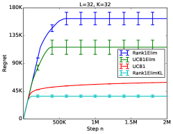
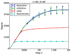
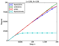
(a)                                                                        (b)                                                                        (c)

Figure 1: The $n$-step regret of ${\tt Rank1ElimKL}$, ${\tt UCB1Elim}$, ${\tt Rank1Elim}$ and ${\tt UCB1}$ on the problem (8) for a. $K=L=32$ b. $K=L=64$ c. $K=L=128$. The results are averaged over $20$ runs.

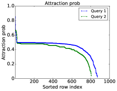
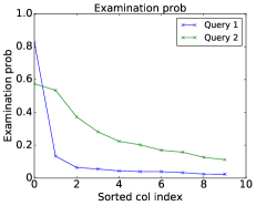
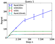
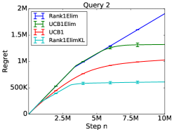
(a)                                                                    (b)                                                                    (c)                                                                    (d)

Figure 2: a. The sorted attraction probabilities of the items from $2$ queries from the Yandex dataset. b. The sorted examination probabilities of the positions for the same $2$ queries. c. The $n$-step regret for Query $1$. d. Regret for Query $2$. The results are averaged over $5$ runs.

The goal of this experiment is to compare ${\tt Rank1ElimKL}$ with three other algorithms from the literature and validate that its regret scales linearly with $K$ and $L$, which implies that it exploits the problem structure. In this experiment, we set $p_{\textsc{u}}=p_{\textsc{v}}=0.25$ and $\Delta_{\textsc{u}}=\Delta_{\textsc{v}}=0.5$ so that $\mu=(1-1/K)0.25+0.75/K=0.25+0.5/K$, $1-p_{\max}=0.25$ and $\gamma=\mu=0.25+0.5/K$. color=Apricot!20,size=,]Cs: Note that $\mu=\gamma$!

In addition to comparing to ${\tt Rank1Elim}$, we also compare to ${\tt UCB1Elim}$ Auer and Ortner (2010) and ${\tt UCB1}$ Auer et al. (2002). ${\tt UCB1}$ is chosen as a baseline as it has been used by Katariya et al. Katariya et al. (2017) in their experiments, too, while ${\tt UCB1Elim}$ is chosen as it is based on a similar elimination approach as ${\tt Rank1Elim}$ and ${\tt Rank1ElimKL}$. We opted not to compare to ${\tt KL\mathchar 45\relax UCB}$ as we expect it to perform similarly to ${\tt UCB1}$ as the problem parameters are relatively close to $0.5$.

Fig. 1 shows the $n$-step regret of ${\tt Rank1ElimKL}$, ${\tt Rank1Elim}$, ${\tt UCB1Elim}$, and ${\tt UCB1}$ as a function of time ($n$) for values of $K=L$, the latter of which double from one plot to the next. We observe that only the regret of ${\tt Rank1ElimKL}$ flattens in all three problems. We also see that the regret of ${\tt Rank1ElimKL}$ doubles as $K$ and $L$ double, indicating that our bound in Theorem 1 has the right scaling in $K+L$, and that the algorithm leverages the problem structure. On the other hand, the regret of ${\tt UCB1}$ and ${\tt UCB1Elim}$ quadruples when $K$ and $L$ double, because their regret is $\Omega(KL)$. Finally, in all problems, we observe that ${\tt Rank1ElimKL}$ outperforms all other algorithms, which indicates that it leverages the structure of the problem in an efficient manner. This is most obvious for large $K$ and $L$, e.g., Fig. 1c. This happens because ${\tt Rank1ElimKL}$ works with improved confidence intervals. It is worth noting that $\mu=\gamma$ for this problem, and hence $\mu^{2}=\mu\gamma$, and according to Theorem 1, ${\tt Rank1ElimKL}$ should not perform better than ${\tt Rank1Elim}$, yet it is $4$ times better as seen in Fig. 1. This suggests that our upper bound is loose.

5.2 Models based on Real-World Data

In this experiment, we compare the performance of ${\tt Rank1ElimKL}$ and other algorithms on models derived from the Yandex dataset Yandex (2013), an anonymized search log of $35$M search sessions. Each session contains a query, the list of displayed documents at positions $1$ to $10$, and the clicks on those documents. We extract the $20$ most frequent queries from the dataset, and estimate the parameters of the PBM model using the EM algorithm Markov (2014); Chuklin et al. (2015).

In order to illustrate the typical models we obtain, we plot the learned parameters of two queries, Queries $1$ and $2$. Fig. 2a shows the sorted attraction probabilities of items in the queries, and Fig. 2b shows the sorted examination probabilities of the positions. Query $1$ has $L=871$ items and Query $2$ has $L=807$ items. We illustrate the performance on these queries because they differ notably in their $\mu$ (3) and $p_{\max}$ (4), so we can study the performance of our algorithm in different real-world settings. Fig. 2c and d show the regret of all algorithms on Queries $1$ and $2$, respectively.

For Query $1$, ${\tt Rank1ElimKL}$ is significantly better than ${\tt Rank1Elim}$ and ${\tt UCB1Elim}$, and no worse than ${\tt UCB1}$. For Query $2$, ${\tt Rank1ElimKL}$ is superior to all algorithms. Note that $p_{\max}=0.85$ in Query $1$ is higher than $p_{\max}=0.66$ in Query $2$. Also, $\mu=0.13$ in Query $1$ is lower than $\mu=0.28$ in Query $2$. From Eq. 5, $\gamma=0.15$ for Query $1$, which is lower than $\gamma=0.34$ for Query $2$. Our upper bound (Theorem 1) on the regret of ${\tt Rank1ElimKL}$ scales as $\mathcal{O}((\mu\gamma)^{-1})$, and consequently we expect ${\tt Rank1ElimKL}$ to perform better on Query $2$. The results confirm this expectation.

Fig. 3 shows the regret averaged over all $20$ queries. Here we compute the average regret on the $20$ queries, and calculate the standard error over $5$ runs. ${\tt Rank1ElimKL}$ has the lowest regret among all the algorithms; its regret is $10.9$ percent lower than that of ${\tt UCB1}$, and $79$ percent lower than that of ${\tt Rank1Elim}$. This is expected: Some real-world instances have a benign rank-$1$ structure like Query $2$, while others do not, like Query $1$. Hence we see a reduction in the average gains of ${\tt Rank1ElimKL}$ over ${\tt UCB1}$ in Fig. 3 as compared to Fig. 2d. The high regret of ${\tt Rank1Elim}$, which also is designed to exploit the problem structure, shows that it fails when faced with such unfavorable rank-$1$ problems. The fact that ${\tt Rank1ElimKL}$ performs on-par with optimal algorithms on the hard problems, and is able to better leverage the problem structure on easy ones, makes it an appealing solution for practice.

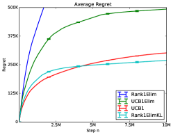
Figure 3: The average $n$-step regret over all $20$ queries from the Yandex dataset, with $5$ runs per query.

6 Related Work

Our algorithm is based on the ${\tt Rank1Elim}$ algorithm of Katariya et al. Katariya et al. (2017); the main difference being that we replace the confidence intervals of ${\tt Rank1Elim}$ that are based on subgaussian tail inequalities with confidence intervals based on KL divergences. As discussed beforehand, this result in an unilateral improvement of their regret bound: The new algorithm is still able to exploit the problem structure of benign instances, while, unlike for ${\tt Rank1Elim}$, its regret is still controlled even on instances that are “hard” for ${\tt Rank1Elim}$. As demonstrated in the previous section, the new algorithm is also a major practical improvement over ${\tt Rank1Elim}$, while staying competitive with alternatives on hard instances.

Several other papers studied bandits where the payoff is given by a low rank matrix. Zhao et al. Zhao et al. (2013) proposed a bandit algorithm for low-rank matrix completion, which approximates the posterior of latent item features by a single point. The authors do not analyze this algorithm. Kawale et al. Kawale et al. (2015) proposed a bandit algorithm for low-rank matrix completion which uses Thompson sampling with Rao-Blackwellization. They analyze a variant of their algorithm whose $n$-step regret for rank-$1$ matrices is $O((1/\Delta^{2})\log n)$. This is suboptimal compared to our algorithm. Maillard et al. Maillard and Mannor (2014) studied a multi-armed bandit problem where the arms are partitioned into several latent groups. In this work, we do not make any such assumptions, but our results are limited to rank $1$. Gentile et al. Gentile et al. (2014) proposed an algorithm that clusters users based on their preferences, under the assumption that the features of items are known. Sen et al. Sen et al. (2017) proposed an algorithm for contextual bandits with latent confounders, which reduces to a multi-armed bandit problem where the reward matrix is low-rank. They use an NMF-based approach and require that the reward matrix obeys a variant of the restricted isometry property. We make no such assumptions. Our work also differs from all above papers in the setting. The learning agents controls both the choice of the row and column. In the above papers, the rows are controlled by the environment.

${\tt Rank1ElimKL}$ is motivated by the structure of the PBM Richardson et al. (2007). Lagree et al. Lagree et al. (2016) proposed a bandit algorithm for this model but they assume that the examination probabilities are known. ${\tt Rank1ElimKL}$ can be used to solve this problem without this assumption. The cascade model Craswell et al. (2008) is an alternative way of explaining the position bias in click data Chuklin et al. (2015). Bandit algorithms for this class of models have been proposed in several recent papers Kveton et al. (2015a); Combes et al. (2015); Kveton et al. (2015b); Katariya et al. (2016); Zong et al. (2016); Li et al. (2016).

7 Conclusions

In this work, we proposed ${\tt Rank1ElimKL}$, an elimination based algorithm that uses ${\tt KL\mathchar 45\relax UCB}$ confidence intervals to find the maximum entry of a stochastic rank-$1$ matrix with Bernoulli rewards. The algorithm is a modification of the ${\tt Rank1Elim}$ algorithm Katariya et al. (2017) where the subgaussian-type confidence intervals are replaced by ones that use KL divergences. As we demonstrate both empirically and analytically, this change results in a significant improvement. As a result, we obtain the first algorithm that is able to exploit the rank-1 structure without paying a significant penalty on instances where the rank-1 structure cannot be exploited.

Finally, we note that ${\tt Rank1ElimKL}$ uses the rank-$1$ structure of the problem and there are no guarantees beyond rank $1$. While the dependence of the regret of ${\tt Rank1ElimKL}$ on $1/\Delta$ is known to be tight Katariya et al. (2017), the question about the optimal dependence on $1/\mu$ is still open.

Appendix A Proof of Theorem 1

We start by recalling Theorem 10 of Garivier and Cappe Garivier and Cappe [2011] with a slight extension that follows immediately by inspecting their proof. We will comment on the difference after stating the definitions. Let $(X_{t})_{t\geq 1}$ be a sequence of random variables bounded in $[0,1]$. Assume that $(\mathcal{F}_{t})_{t\geq 1}$ is a filtration ($\mathcal{F}_{t}\subset\mathcal{F}_{t+1}$ are $\sigma$-algebras) and $(X_{t})_{t\geq 1}$ is $(\mathcal{F}_{t})_{t}$-adapted (i.e., for $t\geq 1$, $X_{1},\dots,X_{t}$ are $\mathcal{F}_{t}$ measurable), and $\mathbb{E}\left[X_{t+1}|\mathcal{F}_{t}\right]=\mu$ with some fixed value $\mu\in[0,1]$. Let $(\varepsilon_{t})_{t\geq 1}$ be a sequence of $(\mathcal{F}_{t})$-previsible Bernoulli random variables: For all $t\geq 1$, $\varepsilon_{t}$ is $\mathcal{F}_{t-1}$-measurable with $\mathcal{F}_{0}=\mathcal{F}$ the $\sigma$-algebra that holds all random variables. Define

$$S(t) =\sum_{s=1}^{t}\varepsilon_{s}X_{s}\,,\quad N(t)=\sum_{s=1}^{t}\varepsilon_{s}\,,\quad\hat{\mu}(t)=\frac{S(t)}{N(t)}\,,\quad t\geq 1\,.$$

The difference to the assumptions used by Garivier and Cappe Garivier and Cappe [2011] is that they assume that the random variables $(X_{t})_{t\geq 1}$ are independent with common mean $\mu$ and that for $s>t$, $X_{s}$ is independent of $\mathcal{F}_{t}$. With this we are ready to state their theorem:

Theorem 2 (After Theorem 10 of Garivier and Cappe Garivier and Cappe [2011]).

Let $(\hat{\mu}(t))_{t\geq 1}$ be as above and let

$$U(t)=\sup\{\,q>\hat{\mu}(t)\,:\,N(t)\,d(\hat{\mu}(t),q)\leq\delta\,\}\,.$$

Then,

$$P(U(t)<\mu)\leq e\,\lceil\delta\log(t)\rceil\exp(-\delta)\,.$$

Let us now turn to our proof. Let $\mathbf{R}^{\textsc{u}}_{\ell}(i)$ be the stochastic regret associated with row $i$ in row exploration stage $\ell$ and $\mathbf{R}^{\textsc{v}}_{\ell}(j)$ be the stochastic regret associated with column $j$ in column exploration stage $\ell$. Then the expected $n$-step regret of ${\tt Rank1ElimKL}$ can be written as

$$R(n)\leq\mathbb{E}\left[\sum_{\ell=0}^{n-1}\left(\sum_{i=1}^{K}\mathbf{R}^{\textsc{u}}_{\ell}(i)+\sum_{j=1}^{L}\mathbf{R}^{\textsc{v}}_{\ell}(j)\right)\right]\,,$$

where the outer sum is over possibly $n$ stages. Let

$$\mathcal{E}^{\textsc{u}}_{\ell}=\{\text{Event $1$: } \forall i\in\mathbf{I}_{\ell}:\bar{\mathbf{u}}_{\ell}(i)\in[\mathbf{L}^{\textsc{u}}_{\ell}(i),\mathbf{U}^{\textsc{u}}_{\ell}(i)]\,,$$

Event $$2 \forall i\in\mathbf{I}_{\ell}:\bar{\mathbf{u}}_{\ell}(i)\geq\mu\bar{u}(i)\,,$$:

Event $$3 \forall i\in\mathbf{I}_{\ell}\setminus\left\{i^{\ast}\right\}:n_{\ell}\geq\frac{16}{\mu\gamma(\Delta^{\textsc{u}}_{i})^{2}}\log n\implies\hat{\mathbf{u}}(i)\leq\mathbf{c}_{\ell}[\bar{u}(i)+\Delta^{\textsc{u}}_{i}/4]\,,$$:

Event $$4 \forall i\in\mathbf{I}_{\ell}\setminus\left\{i^{\ast}\right\}:n_{\ell}\geq\frac{16}{\mu\gamma(\Delta^{\textsc{u}}_{i})^{2}}\log n\implies\hat{\mathbf{u}}(i^{\ast})\geq\mathbf{c}_{\ell}[\bar{u}(i^{\ast})-\Delta^{\textsc{u}}_{i}/4]\}$$:

be “good events” associated with row $i$ at the end of stage $\ell$, where

$$\bar{\mathbf{u}}_{\ell}(i)=\sum_{t=0}^{\ell}\mathbb{E}\left[\sum_{j=1}^{L}\frac{\mathbf{C}^{\textsc{u}}_{t}(i,j)-\mathbf{C}^{\textsc{u}}_{t-1}(i,j)}{n_{\ell}}\,\middle|\,\mathbf{h}^{\textsc{v}}_{t}\right]=\underbrace{\left(\sum_{t=0}^{\ell}\frac{n_{t}-n_{t-1}}{n_{\ell}}\sum_{j=1}^{L}\frac{\bar{v}(\mathbf{h}^{\textsc{v}}_{t}(j))}{L}\right)}_{\mathbf{c}_{\ell}}\bar{u}(i)$$

is the expected reward of row $i$ conditioned on column elimination strategy $\mathbf{h}^{\textsc{v}}_{0},\dots,\mathbf{h}^{\textsc{v}}_{\ell}$; $\mathbf{C}^{\textsc{u}}_{-1}(i,j)=0$; and $n_{-1}=0$. Let $\overline{\mathcal{E}^{\textsc{u}}_{\ell}}$ be the complement of event $\mathcal{E}^{\textsc{u}}_{\ell}$. Let

$$\mathcal{E}^{\textsc{v}}_{\ell}=\{\text{Event $1$: } \forall j\in\mathbf{J}_{\ell}:\bar{\mathbf{v}}_{\ell}(j)\in[\mathbf{L}^{\textsc{v}}_{\ell}(j),\mathbf{U}^{\textsc{v}}_{\ell}(j)]\,,$$

Event $$2 \forall j\in\mathbf{J}_{\ell}:\bar{\mathbf{v}}_{\ell}(j)\geq\mu\bar{v}(j)\,,$$:

Event $$3 \forall j\in\mathbf{J}_{\ell}\setminus\left\{j^{\ast}\right\}:n_{\ell}\geq\frac{16}{\mu\gamma(\Delta^{\textsc{v}}_{j})^{2}}\log n\implies\hat{\mathbf{v}}(j)\leq\mathbf{c}_{\ell}[\bar{v}(j)+\Delta^{\textsc{v}}_{j}/4]\,,$$:

Event $$4 \forall j\in\mathbf{J}_{\ell}\setminus\left\{j^{\ast}\right\}:n_{\ell}\geq\frac{16}{\mu\gamma(\Delta^{\textsc{v}}_{j})^{2}}\log n\implies\hat{\mathbf{v}}(j^{\ast})\geq\mathbf{c}_{\ell}[\bar{v}(j^{\ast})-\Delta^{\textsc{v}}_{j}/4]\}$$:

be “good events” associated with column $j$ at the end of stage $\ell$, where

$$\bar{\mathbf{v}}_{\ell}(j)=\sum_{t=0}^{\ell}\mathbb{E}\left[\sum_{i=1}^{K}\frac{\mathbf{C}^{\textsc{v}}_{t}(i,j)-\mathbf{C}^{\textsc{v}}_{t-1}(i,j)}{n_{\ell}}\,\middle|\,\mathbf{h}^{\textsc{u}}_{t}\right]=\underbrace{\left(\sum_{t=0}^{\ell}\frac{n_{t}-n_{t-1}}{n_{\ell}}\sum_{i=1}^{K}\frac{\bar{u}(\mathbf{h}^{\textsc{u}}_{t}(i))}{K}\right)}_{\mathbf{c}_{\ell}}\bar{v}(j)$$

is the expected reward of column $j$ conditioned on row elimination strategy $\mathbf{h}^{\textsc{u}}_{0},\dots,\mathbf{h}^{\textsc{u}}_{\ell}$; $\mathbf{C}^{\textsc{v}}_{-1}(i,j)=0$; and $n_{-1}=0$. Let $\overline{\mathcal{E}^{\textsc{v}}_{\ell}}$ be the complement of event $\mathcal{E}^{\textsc{v}}_{\ell}$. Let $\mathcal{E}$ be the event that all events $\mathcal{E}^{\textsc{u}}_{\ell}$ and $\mathcal{E}^{\textsc{v}}_{\ell}$ happen; and $\overline{\mathcal{E}}$ be the complement of $\mathcal{E}$, the event that at least one of $\mathcal{E}^{\textsc{u}}_{\ell}$ and $\mathcal{E}^{\textsc{v}}_{\ell}$ does not happen. Then the expected $n$-step regret can be bounded from above as

$$R(n) \leq\mathbb{E}\left[\left(\sum_{\ell=0}^{n-1}\left(\sum_{i=1}^{K}\mathbf{R}^{\textsc{u}}_{\ell}(i)+\sum_{j=1}^{L}\mathbf{R}^{\textsc{v}}_{\ell}(j)\right)\right)\mathds{1}\!\left\{\mathcal{E}\right\}\right]+nP(\overline{\mathcal{E}})$$

$$\leq\mathbb{E}\left[\left(\sum_{\ell=0}^{n-1}\left(\sum_{i=1}^{K}\mathbf{R}^{\textsc{u}}_{\ell}(i)+\sum_{j=1}^{L}\mathbf{R}^{\textsc{v}}_{\ell}(j)\right)\right)\mathds{1}\!\left\{\mathcal{E}\right\}\right]+(K+L)(6e+2)$$

$$=\sum_{i=1}^{K}\mathbb{E}\left[\sum_{\ell=0}^{n-1}\mathbf{R}^{\textsc{u}}_{\ell}(i)\mathds{1}\!\left\{\mathcal{E}\right\}\right]+\sum_{j=1}^{L}\mathbb{E}\left[\sum_{\ell=0}^{n-1}\mathbf{R}^{\textsc{v}}_{\ell}(j)\mathds{1}\!\left\{\mathcal{E}\right\}\right]+(K+L)(6e+2)\,,$$

where the second inequality is from Lemma 2.

Let $\mathcal{H}_{\ell}=(\mathbf{I}_{\ell},\mathbf{J}_{\ell})$ be the rows and columns in stage $\ell$, and

$$\mathcal{F}_{\ell}=\left\{\forall i\in\mathbf{I}_{\ell}:\sqrt{\mu\gamma}\Delta^{\textsc{u}}_{i}\leq\tilde{\Delta}_{\ell-1},\ \forall j\in\mathbf{J}_{\ell}:\sqrt{\mu\gamma}\Delta^{\textsc{v}}_{j}\leq\tilde{\Delta}_{\ell-1}\right\}$$

be the event that all rows and columns with “large gaps” are eliminated by the beginning of stage $\ell$. By Lemma 3, event $\mathcal{F}_{\ell}$ happens when event $\mathcal{E}$ happens. Moreover, the expected regret in stage $\ell$ is independent of $\mathcal{F}_{\ell}$ given $\mathcal{H}_{\ell}$. Therefore, we can bound the regret from above as

$$R(n)\leq\sum_{i=1}^{K}\mathbb{E}\left[\sum_{\ell=0}^{n-1}\mathbb{E}\left[\mathbf{R}^{\textsc{u}}_{\ell}(i)\,\middle|\,\mathcal{H}_{\ell}\right]\mathds{1}\!\left\{\mathcal{F}_{\ell}\right\}\right]+\sum_{j=1}^{L}\mathbb{E}\left[\sum_{\ell=0}^{n-1}\mathbb{E}\left[\mathbf{R}^{\textsc{v}}_{\ell}(j)\,\middle|\,\mathcal{H}_{\ell}\right]\mathds{1}\!\left\{\mathcal{F}_{\ell}\right\}\right]+(K+L)(6e+2)\,.$$ (9)

By Lemma 4,

$$\mathbb{E}\left[\sum_{\ell=0}^{n-1}\mathbb{E}\left[\mathbf{R}^{\textsc{u}}_{\ell}(i)\,\middle|\,\mathcal{H}_{\ell}\right]\mathds{1}\!\left\{\mathcal{F}_{\ell}\right\}\right] \leq\frac{160}{\mu\gamma\bar{\Delta}^{\textsc{u}}_{i}}\log n+80\,,$$

$$\mathbb{E}\left[\sum_{\ell=0}^{n-1}\mathbb{E}\left[\mathbf{R}^{\textsc{v}}_{\ell}(j)\,\middle|\,\mathcal{H}_{\ell}\right]\mathds{1}\!\left\{\mathcal{F}_{\ell}\right\}\right] \leq\frac{160}{\mu\gamma\bar{\Delta}^{\textsc{v}}_{j}}\log n+80\,.$$

Now we apply the above upper bounds to (9) and get our main claim.

Appendix B Technical Lemmas

Lemma 2.

Let $\overline{\mathcal{E}}$ be defined as in the proof of Theorem 1. Then for any $n\geq 5$,

$$P(\overline{\mathcal{E}})\leq\frac{(K+L)(6e+2)}{n}\,.$$

Proof.

Let $\mathcal{E}_{\ell}=\mathcal{E}^{\textsc{u}}_{\ell}\cap\mathcal{E}^{\textsc{v}}_{\ell}$. Then, $\overline{\mathcal{E}}=\overline{\mathcal{E}_{0}}\cup(\overline{\mathcal{E}_{1}}\cap\mathcal{E}_{0})\cup\dots\cup(\overline{\mathcal{E}_{n-1}}\cap\mathcal{E}_{0}\cap\dots\cap\mathcal{E}_{n-2})$. By the same logic, $\overline{\mathcal{E}_{\ell}}\cap\mathcal{E}_{0}\cap\dots\cap\mathcal{E}_{\ell-1}=(\overline{\mathcal{E}^{\textsc{u}}_{\ell}}\cap\mathcal{E}_{0}\cap\dots\cap\mathcal{E}_{\ell-1})\cup(\overline{\mathcal{E}^{\textsc{v}}_{\ell}}\cap\mathcal{E}^{\textsc{u}}_{\ell}\cap\mathcal{E}_{0}\cap\dots\cap\mathcal{E}_{\ell-1})$. Hence,

$$P(\overline{\mathcal{E}})\leq\sum_{\ell=0}^{n-1}P(\overline{\mathcal{E}^{\textsc{u}}_{\ell}},\mathcal{E}_{0},\dots,\mathcal{E}_{\ell-1})+P(\overline{\mathcal{E}^{\textsc{v}}_{\ell}},\mathcal{E}_{0},\dots,\mathcal{E}_{\ell-1})\,.$$

Now we bound the probability of the events $\overline{\mathcal{E}^{\textsc{u}}_{\ell}},\mathcal{E}^{\textsc{u}}_{0},\ \dots,\ \mathcal{E}^{\textsc{u}}_{\ell-1},\mathcal{E}^{\textsc{v}}_{0},\ \dots,\ \mathcal{E}^{\textsc{v}}_{\ell-1}$; and then sum them up. The proof for the probability of the second term above is analogous and hence it is omitted.

Event $1$

The probability that event $1$ in $\mathcal{E}^{\textsc{u}}_{\ell}$ does not happen is bounded as follows. For any $i\in[K]$ and $\mathbf{h}^{\textsc{v}}_{0},\dots,\mathbf{h}^{\textsc{v}}_{\ell}$,

$$P(\bar{\mathbf{u}}_{\ell}(i)\notin[\mathbf{L}^{\textsc{u}}_{\ell}(i),\mathbf{U}^{\textsc{u}}_{\ell}(i)]) \leq P(\bar{\mathbf{u}}_{\ell}(i)<\mathbf{L}^{\textsc{u}}_{\ell}(i))+P(\bar{\mathbf{u}}_{\ell}(i)>\mathbf{U}^{\textsc{u}}_{\ell}(i))$$

$$\leq\frac{2e\left\lceil\log(n\log^{3}n)\log n_{\ell}\right\rceil}{n\log^{3}n}$$

$$\leq\frac{2e\left\lceil\log^{2}n+\log(\log^{3}n)\log n\right\rceil}{n\log^{3}n}$$

$$\leq\frac{2e\left\lceil 2\log^{2}n\right\rceil}{n\log n}$$

$$\leq\frac{6e}{n\log n}\,,$$

where the second inequality is from Theorem 2, color=Apricot!20,size=,]Cs: Clearly, we need to extend their result because in our case the conditional means shift over time. the third inequality is from $n\geq n_{\ell}$, the fourth inequality is from $\log(\log^{3}n)\leq\log n$ for $n\geq 5$, and the last inequality is from $\left\lceil 2\log^{2}n\right\rceil\leq 3\log^{2}n$ for $n\geq 3$. By the union bound,

$$P(\exists i\in\mathbf{I}_{\ell}\text{ s.t. }\bar{\mathbf{u}}_{\ell}(i)\notin[\mathbf{L}^{\textsc{u}}_{\ell}(i),\mathbf{U}^{\textsc{u}}_{\ell}(i)])\leq\frac{6eK}{n\log n}$$

for any $\mathbf{I}_{\ell}$ and $\mathbf{h}^{\textsc{v}}_{0},\dots,\mathbf{h}^{\textsc{v}}_{\ell}$. Finally, we take the expectation over $\mathbf{I}_{\ell}$ and $\mathbf{h}^{\textsc{v}}_{0},\dots,\mathbf{h}^{\textsc{v}}_{\ell}$; and have that the probability that event $1$ in $\mathcal{E}^{\textsc{u}}_{\ell}$ does not happen at the end of stage $\ell$ is bounded as above.

Event $2$

Event $2$ in $\mathcal{E}^{\textsc{u}}_{\ell}$ is guaranteed to happen, $\bar{\mathbf{u}}_{\ell}(i)\geq\mu\bar{u}(i)$ for all $i\in\mathbf{I}_{\ell}$. This claim holds trivially when $\ell=0$, because all columns in row elimination stage $0$ are chosen with the same probability. When $\ell>0$, all column confidence intervals up to stage $\ell$ hold because events $\mathcal{E}^{\textsc{v}}_{0},\dots,\mathcal{E}^{\textsc{v}}_{\ell-1}$ happen. Therefore, by the design of ${\tt Rank1ElimKL}$, any eliminated column $j$ up to stage $\ell$ is substituted with column $j^{\prime}$ such that $\bar{v}(j^{\prime})\geq\allowbreak\bar{v}(j)$. Since the columns in any row elimination stage are chosen randomly, $\bar{\mathbf{u}}_{\ell}(i)\geq\mu\bar{u}(i)$ for all $i\in\mathbf{I}_{\ell}$.

Event $3$

The probability that event $3$ in $\mathcal{E}^{\textsc{u}}_{\ell}$ does not happen is bounded as follows. If the event does not happen in row $i$, then

$$n_{\ell}\geq\frac{16}{\mu\gamma(\Delta^{\textsc{u}}_{i})^{2}}\log n\,,\quad\hat{\mathbf{u}}(i)>\mathbf{c}_{\ell}[\bar{u}(i)+\Delta^{\textsc{u}}_{i}/4]\,.$$

From Hoeffding’s inequality and $\mathbb{E}\left[\hat{\mathbf{u}}(i)\right]=\mathbf{c}_{\ell}\bar{u}(i)$, we have that

$$P(\hat{\mathbf{u}}(i)>\mathbf{c}_{\ell}[\bar{u}(i)+\Delta^{\textsc{u}}_{i}/4])\leq\exp[-n_{\ell}d(\mathbf{c}_{\ell}[\bar{u}(i)+\Delta^{\textsc{u}}_{i}/4],\mathbf{c}_{\ell}\bar{u}(i))]\,.$$

From our scaling lemma (Lemma 1), the inequality $\mathbf{c}_{\ell}\geq\mu$ and the definition $\gamma=\max(\mu,1-p_{\max})$, we have that

$$\exp[-n_{\ell}d(\mathbf{c}_{\ell}[\bar{u}(i)+\Delta^{\textsc{u}}_{i}/4],\mathbf{c}_{\ell}\bar{u}(i))] \leq\exp[-n_{\ell}\,\mu\gamma\,(\Delta^{\textsc{u}}_{i})^{2}/8]\,.$$

Finally, from our assumption on $n_{\ell}$, we conclude that

$$\exp[-n_{\ell}\mu\gamma(\Delta^{\textsc{u}}_{i})^{2}/8]\leq\exp[-2\log n]=\frac{1}{n^{2}}\,.$$

Now we chain all inequalities and observe that event $3$ in $\mathcal{E}^{\textsc{u}}_{\ell}$ does not happen with probability of at most $K/n^{2}$ for any $\mathbf{I}_{\ell}$ and $\mathbf{h}^{\textsc{v}}_{0},\dots,\mathbf{h}^{\textsc{v}}_{\ell}$. Finally, we take the expectation over $\mathbf{I}_{\ell}$ and $\mathbf{h}^{\textsc{v}}_{0},\dots,\mathbf{h}^{\textsc{v}}_{\ell}$; and have that the probability that event $3$ in $\mathcal{E}^{\textsc{u}}_{\ell}$ does not happen at the end of stage $\ell$ is at most $K/n^{2}$.

Event $4$

The probability that event $4$ in $\mathcal{E}^{\textsc{u}}_{\ell}$ does not happen can be bounded similarly to that of event $3$. If the event does not happen in row $i$, then

$$n_{\ell}\geq\frac{16}{\mu\gamma(\Delta^{\textsc{u}}_{i})^{2}}\log n\,,\quad\hat{\mathbf{u}}(i^{\ast})<\mathbf{c}_{\ell}[\bar{u}(i^{\ast})-\Delta^{\textsc{u}}_{i}/4]\,.$$

Then by the same reasoning as in event $3$,

$$P(\hat{\mathbf{u}}(i^{\ast})<\mathbf{c}_{\ell}[\bar{u}(i^{\ast})-\Delta^{\textsc{u}}_{i}/4]) \leq\exp[-n_{\ell}d(\mathbf{c}_{\ell}[\bar{u}(i^{\ast})-\Delta^{\textsc{u}}_{i}/4],\mathbf{c}_{\ell}\bar{u}(i^{\ast}))]$$

$$\leq\exp[-n_{\ell}\mu\gamma(\Delta^{\textsc{u}}_{i})^{2}/8]$$

$$\leq\exp[-2\log n]$$

$$=\frac{1}{n^{2}}\,.$$

This implies that event $4$ in $\mathcal{E}^{\textsc{u}}_{\ell}$ does not happen with probability of at most $K/n^{2}$ for any $\mathbf{I}_{\ell}$ and $\mathbf{h}^{\textsc{v}}_{0},\dots,\mathbf{h}^{\textsc{v}}_{\ell}$. Finally, we take the expectation over $\mathbf{I}_{\ell}$ and $\mathbf{h}^{\textsc{v}}_{0},\dots,\mathbf{h}^{\textsc{v}}_{\ell}$; and have that the probability that event $4$ in $\mathcal{E}^{\textsc{u}}_{\ell}$ does not happen at the end of stage $\ell$ is at most $K/n^{2}$ .

Total probability

Note that the maximum number of stages in ${\tt Rank1ElimKL}$ is $\log n$. By the union bound, we get that

$$P(\overline{\mathcal{E}}) \leq\left(\frac{6eK}{n\log n}+\frac{K}{n^{2}}+\frac{K}{n^{2}}\right)\log n+\left(\frac{6eL}{n\log n}+\frac{L}{n^{2}}+\frac{L}{n^{2}}\right)\log n$$

$$\leq\frac{(K+L)(6e+2)}{n}\,.$$

This concludes our proof.  

Lemma 3.

Let event $\mathcal{E}$ happen and $m$ be the first stage where $\tilde{\Delta}_{m}<\sqrt{\mu\gamma}\Delta^{\textsc{u}}_{i}$. Then row $i$ must be eliminated by the end of stage $m$. Moreover, let $m$ be the first stage where $\tilde{\Delta}_{m}<\sqrt{\mu\gamma}\Delta^{\textsc{v}}_{j}$. Then column $j$ must be eliminated by the end of stage $m$.

Proof.

We only prove the first claim. The other claim is proved analogously.

From the definition of $n_{m}$ and our assumption on $\tilde{\Delta}_{m}$,

$$n_{m}\geq\frac{16}{\tilde{\Delta}_{m}^{2}}\log n>\frac{16}{\mu\gamma(\Delta^{\textsc{u}}_{i})^{2}}\log n\,.$$ (10)

Suppose that $\mathbf{U}^{\textsc{u}}_{m}(i)\geq\mathbf{c}_{m}[\bar{u}(i)+\Delta^{\textsc{u}}_{i}/2]$ happens. Then from this assumption, the definition of $\mathbf{U}^{\textsc{u}}_{m}(i)$, and event $3$ in $\mathcal{E}^{\textsc{u}}_{m}$,

$$d(\hat{\mathbf{u}}(i),\mathbf{U}^{\textsc{u}}_{m}(i)) \geq d^{+}(\hat{\mathbf{u}}(i),\mathbf{c}_{m}[\bar{u}(i)+\Delta^{\textsc{u}}_{i}/2])$$

$$\geq d(\mathbf{c}_{m}[\bar{u}(i)+\Delta^{\textsc{u}}_{i}/4],\mathbf{c}_{m}[\bar{u}(i)+\Delta^{\textsc{u}}_{i}/2])\,,$$

where $d^{+}(p,q)=d(p,q)\mathds{1}\!\left\{p\leq q\right\}$. From our scaling lemma (Lemma 1), the inequality $\mathbf{c}_{\ell}\geq\mu$ and the definition $\gamma=\max(\mu,1-p_{\max})$, we further have that

$$d(\mathbf{c}_{m}[\bar{u}(i)+\Delta^{\textsc{u}}_{i}/4],\mathbf{c}_{m}[\bar{u}(i)+\Delta^{\textsc{u}}_{i}/2]) \geq\frac{\mu\gamma\,(\Delta^{\textsc{u}}_{i})^{2}}{8}\,.$$

From the definition of $\mathbf{U}^{\textsc{u}}_{m}(i)$ and above inequalities,

$$n_{m}=\frac{2\log n}{d(\hat{\mathbf{u}}(i),\mathbf{U}^{\textsc{u}}_{m}(i))}\leq\frac{16\log n}{\mu\gamma(\Delta^{\textsc{u}}_{i})^{2}}\,.$$

This contradicts to (10), and therefore it must be true that $\mathbf{U}^{\textsc{u}}_{m}(i)<\mathbf{c}_{m}[\bar{u}(i)+\Delta^{\textsc{u}}_{i}/2]$.

Now suppose that $\mathbf{L}^{\textsc{u}}_{m}(i^{\ast})\leq\mathbf{c}_{m}[\bar{u}(i^{\ast})-\Delta^{\textsc{u}}_{i}/2]$ happens. Then from this assumption, the definition of $\mathbf{L}^{\textsc{u}}_{m}(i^{\ast})$, and event $4$ in $\mathcal{E}^{\textsc{u}}_{m}$,

$$d(\hat{\mathbf{u}}(i^{\ast}),\mathbf{L}^{\textsc{u}}_{m}(i^{\ast})) \geq d^{-}(\hat{\mathbf{u}}(i^{\ast}),\mathbf{c}_{m}[\bar{u}(i^{\ast})-\Delta^{\textsc{u}}_{i}/2])$$

$$\geq d(\mathbf{c}_{m}[\bar{u}(i^{\ast})-\Delta^{\textsc{u}}_{i}/4],\mathbf{c}_{m}[\bar{u}(i^{\ast})-\Delta^{\textsc{u}}_{i}/2])\,,$$

where $d^{-}(p,q)=d(p,q)\mathds{1}\!\left\{p\geq q\right\}$. From our scaling lemma (Lemma 1), the inequality $\mathbf{c}_{\ell}\geq\mu$ and the definition $\gamma=\max(\mu,1-p_{\max})$, we further have that

$$d(\mathbf{c}_{m}[\bar{u}(i^{\ast})-\Delta^{\textsc{u}}_{i}/4],\mathbf{c}_{m}[\bar{u}(i^{\ast})-\Delta^{\textsc{u}}_{i}/2]) \geq\frac{\mu\gamma\,(\Delta^{\textsc{u}}_{i})^{2}}{8}\,.$$

From the definition of $\mathbf{L}^{\textsc{u}}_{m}(i^{\ast})$ and above inequalities,

$$n_{m}=\frac{2\log n}{d(\hat{\mathbf{u}}(i^{\ast}),\mathbf{L}^{\textsc{u}}_{m}(i^{\ast}))}\leq\frac{16\log n}{\mu\gamma(\Delta^{\textsc{u}}_{i})^{2}}\,.$$

This contradicts to (10), and therefore it must be true that $\mathbf{L}^{\textsc{u}}_{m}(i^{\ast})>\mathbf{c}_{m}[\bar{u}(i^{\ast})-\Delta^{\textsc{u}}_{i}/2]$.

Finally, it follows that row $i$ is eliminated by the end of stage $m$ because

$$\mathbf{U}^{\textsc{u}}_{m}(i)<\mathbf{c}_{m}[\bar{u}(i)+\Delta^{\textsc{u}}_{i}/2]=\mathbf{c}_{m}[\bar{u}(i^{\ast})-\Delta^{\textsc{u}}_{i}/2]<\mathbf{L}^{\textsc{u}}_{m}(i^{\ast})\,.$$

This concludes our proof.  

Lemma 4.

The expected regret associated with any row $i\in[K]$ is bounded as

$$\mathbb{E}\left[\sum_{\ell=0}^{n-1}\mathbb{E}\left[\mathbf{R}^{\textsc{u}}_{\ell}(i)\,\middle|\,\mathcal{H}_{\ell}\right]\mathds{1}\!\left\{\mathcal{F}_{\ell}\right\}\right]\leq\frac{160}{\mu\gamma\bar{\Delta}^{\textsc{u}}_{i}}\log n+80\,.$$

Moreover, the expected regret associated with any column $j\in[L]$ is bounded as

$$\mathbb{E}\left[\sum_{\ell=0}^{n-1}\mathbb{E}\left[\mathbf{R}^{\textsc{v}}_{\ell}(j)\,\middle|\,\mathcal{H}_{\ell}\right]\mathds{1}\!\left\{\mathcal{F}_{\ell}\right\}\right]\leq\frac{160}{\mu\gamma\bar{\Delta}^{\textsc{v}}_{j}}\log n+80\,.$$

Proof.

We only prove the first claim. The other claim is proved analogously.

This proof has two parts. In the first part, we assume that row $i$ is suboptimal. In the second part, we assume that row $i$ is optimal, $\Delta^{\textsc{u}}_{i}=0$.

Row $i$ is suboptimal

Let row $i$ be suboptimal and $m$ be the first stage where $\tilde{\Delta}_{m}<\sqrt{\mu\gamma}\Delta^{\textsc{u}}_{i}$. Then row $i$ is guaranteed to be eliminated by the end of stage $m$ (Lemma 3), and therefore

$$\mathbb{E}\left[\sum_{\ell=0}^{n-1}\mathbb{E}\left[\mathbf{R}^{\textsc{u}}_{\ell}(i)\,\middle|\,\mathcal{H}_{\ell}\right]\mathds{1}\!\left\{\mathcal{F}_{\ell}\right\}\right]\leq\mathbb{E}\left[\sum_{\ell=0}^{m}\mathbb{E}\left[\mathbf{R}^{\textsc{u}}_{\ell}(i)\,\middle|\,\mathcal{H}_{\ell}\right]\mathds{1}\!\left\{\mathcal{F}_{\ell}\right\}\right]\,.$$

By Lemma 4 of Katariya et al. Katariya et al. [2017], the expected regret of choosing row $i$ in stage $\ell$ can be bounded from above as

$$\mathbb{E}\left[\mathbf{R}^{\textsc{u}}_{\ell}(i)\,\middle|\,\mathcal{H}_{\ell}\right]\mathds{1}\!\left\{\mathcal{F}_{\ell}\right\}\leq(\Delta^{\textsc{u}}_{i}+2^{m-\ell+1}\Delta^{\textsc{u}}_{i})(n_{\ell}-n_{\ell-1})\,,$$

where $n_{\ell}$ is the number of steps by the end of stage $\ell$, $2^{m-\ell+1}\Delta^{\textsc{u}}_{i}$ is an upper bound on the gap of any non-eliminated column in stage $\ell\leq m$, and $n_{-1}=0$. The bound follows from the observation that if column $j$ is not eliminated before stage $\ell$, then

$$\Delta^{\textsc{v}}_{j}\leq\frac{\tilde{\Delta}_{\ell-1}}{\sqrt{\mu\gamma}}=\frac{2^{m-\ell+1}\tilde{\Delta}_{m}}{\sqrt{\mu\gamma}}<2^{m-\ell+1}\Delta^{\textsc{u}}_{i}\,.$$

It follows that

$$\sum_{\ell=0}^{m}(\Delta^{\textsc{u}}_{i}+2^{m-\ell+1}\Delta^{\textsc{u}}_{i})(n_{\ell}-n_{\ell-1}) \leq\Delta^{\textsc{u}}_{i}n_{m}+\Delta^{\textsc{u}}_{i}\sum_{\ell=0}^{m}2^{m-\ell+1}n_{\ell}$$

$$\leq 2^{4}\Delta^{\textsc{u}}_{i}(2^{2m}\log n+1)+2^{4}\Delta^{\textsc{u}}_{i}\sum_{\ell=0}^{m}2^{m-\ell+1}(2^{2m}\log n+1)$$

$$=2^{2m+4}\Delta^{\textsc{u}}_{i}\log n+16\Delta^{\textsc{u}}_{i}+2^{2m+6}\Delta^{\textsc{u}}_{i}\log n+64\Delta^{\textsc{u}}_{i}$$

$$\leq 5\cdot 2^{6}\cdot 2^{2m-2}\Delta^{\textsc{u}}_{i}\log n+80\,.$$

From the definition of $m$, we have that

$$2^{m-1}=\frac{1}{\tilde{\Delta}_{m-1}}\leq\frac{1}{\sqrt{\mu\gamma}\Delta^{\textsc{u}}_{i}}\,.$$

Now we chain all above inequalities and get that

$$\mathbb{E}\left[\sum_{\ell=0}^{n-1}\mathbb{E}\left[\mathbf{R}^{\textsc{u}}_{\ell}(i)\,\middle|\,\mathcal{H}_{\ell}\right]\mathds{1}\!\left\{\mathcal{F}_{\ell}\right\}\right] \leq\sum_{\ell=0}^{m}(\Delta^{\textsc{u}}_{i}+2^{m-\ell+1}\Delta^{\textsc{u}}_{i})(n_{\ell}-n_{\ell-1})$$

$$\leq\frac{160}{\mu\gamma\Delta^{\textsc{u}}_{i}}\log n+80\,.$$

This concludes the first part of our proof.

Row $i$ is optimal

Let row $i$ be optimal and $m$ be the first stage where $\tilde{\Delta}_{m}<\sqrt{\mu\gamma}\Delta^{\textsc{v}}_{\min}$. Then similarly to the first part of the analysis,

$$\mathbb{E}\left[\sum_{\ell=0}^{n-1}\mathbb{E}\left[\mathbf{R}^{\textsc{u}}_{\ell}(i)\,\middle|\,\mathcal{H}_{\ell}\right]\mathds{1}\!\left\{\mathcal{F}_{\ell}\right\}\right]\leq\frac{160}{\mu\gamma\Delta^{\textsc{v}}_{\min}}\log n+80\,.$$

This concludes our proof.

References

- Auer and Ortner [2010] Peter Auer and Ronald Ortner. UCB revisited: Improved regret bounds for the stochastic multi-armed bandit problem. Periodica Mathematica Hungarica, 61(1-2):55–65, 2010.
- Auer et al. [2002] Peter Auer, Nicolo Cesa-Bianchi, and Paul Fischer. Finite-time analysis of the multiarmed bandit problem. Machine Learning, 47:235–256, 2002.
- Chuklin et al. [2015] Aleksandr Chuklin, Ilya Markov, and Maarten de Rijke. Click Models for Web Search. Morgan & Claypool Publishers, 2015.
- Combes et al. [2015] Richard Combes, Stefan Magureanu, Alexandre Proutiere, and Cyrille Laroche. Learning to rank: Regret lower bounds and efficient algorithms. In Proceedings of the 2015 ACM SIGMETRICS International Conference on Measurement and Modeling of Computer Systems, 2015.
- Craswell et al. [2008] Nick Craswell, Onno Zoeter, Michael Taylor, and Bill Ramsey. An experimental comparison of click position-bias models. In Proceedings of the 1st ACM International Conference on Web Search and Data Mining, pages 87–94, 2008.
- Garivier and Cappe [2011] Aurelien Garivier and Olivier Cappe. The KL-UCB algorithm for bounded stochastic bandits and beyond. In Proceeding of the 24th Annual Conference on Learning Theory, pages 359–376, 2011.
- Gentile et al. [2014] Claudio Gentile, Shuai Li, and Giovanni Zappella. Online clustering of bandits. In Proceedings of the 31st International Conference on Machine Learning, pages 757–765, 2014.
- Katariya et al. [2016] Sumeet Katariya, Branislav Kveton, Csaba Szepesvari, and Zheng Wen. DCM bandits: Learning to rank with multiple clicks. In Proceedings of the 33rd International Conference on Machine Learning, 2016.
- Katariya et al. [2017] Sumeet Katariya, Branislav Kveton, Csaba Szepesvari, Claire Vernade, and Zheng Wen. Stochastic rank-1 bandits. In AISTATS, 2017.
- Kawale et al. [2015] Jaya Kawale, Hung Bui, Branislav Kveton, Long Tran-Thanh, and Sanjay Chawla. Efficient Thompson sampling for online matrix-factorization recommendation. In Advances in Neural Information Processing Systems 28, pages 1297–1305, 2015.
- Kveton et al. [2015a] Branislav Kveton, Csaba Szepesvari, Zheng Wen, and Azin Ashkan. Cascading bandits: Learning to rank in the cascade model. In Proceedings of the 32nd International Conference on Machine Learning, 2015.
- Kveton et al. [2015b] Branislav Kveton, Zheng Wen, Azin Ashkan, and Csaba Szepesvari. Combinatorial cascading bandits. In Advances in Neural Information Processing Systems 28, pages 1450–1458, 2015.
- Lagree et al. [2016] Paul Lagree, Claire Vernade, and Olivier Cappe. Multiple-play bandits in the position-based model. CoRR, abs/1606.02448, 2016.
- Li et al. [2016] Shuai Li, Baoxiang Wang, Shengyu Zhang, and Wei Chen. Contextual combinatorial cascading bandits. In Proceedings of the 33rd International Conference on Machine Learning, pages 1245–1253, 2016.
- Maillard and Mannor [2014] Odalric-Ambrym Maillard and Shie Mannor. Latent bandits. In Proceedings of the 31st International Conference on Machine Learning, pages 136–144, 2014.
- Markov [2014] Ilya Markov. Pyclick - click models for web search. https://github.com/markovi/PyClick, 2014.
- Richardson et al. [2007] Matthew Richardson, Ewa Dominowska, and Robert Ragno. Predicting clicks: Estimating the click-through rate for new ads. In Proceedings of the 16th International Conference on World Wide Web, pages 521–530, 2007.
- Sen et al. [2017] Rajat Sen, Karthikeyan Shanmugam, Murat Kocaoglu, Alexandros G Dimakis, and Sanjay Shakkottai. Contextual bandits with latent confounders: An nmf approach. In AISTATS, 2017.
- Yandex [2013] Yandex personalized web search challenge. https://www.kaggle.com/c/yandex-personalized-web-search-challenge, 2013.
- Zhao et al. [2013] Xiaoxue Zhao, Weinan Zhang, and Jun Wang. Interactive collaborative filtering. In Proceedings of the 22nd ACM International Conference on Information and Knowledge Management, pages 1411–1420, 2013.
- Zong et al. [2016] Shi Zong, Hao Ni, Kenny Sung, Nan Rosemary Ke, Zheng Wen, and Branislav Kveton. Cascading bandits for large-scale recommendation problems. In Proceedings of the 32nd Conference on Uncertainty in Artificial Intelligence, 2016.