Multiloop functional renormalization group that sums up all parquet diagrams

Abstract

We present a multiloop flow equation for the four-point vertex in the functional renormalization group (fRG) framework. The multiloop flow consists of successive one-loop calculations and sums up all parquet diagrams to arbitrary order. This provides substantial improvement of fRG computations for the four-point vertex and, consequently, the self-energy. Using the X-ray-edge singularity as an example, we show that solving the multiloop fRG flow is equivalent to solving the (first-order) parquet equations and illustrate this with numerical results.

Introduction.—Two-particle correlations play a fundamental role in the theory of strongly correlated electron systems. Most response functions measured in condensed-matter experiments are two-particle quantities such as optical or magnetic susceptibilities. The behavior of the two-particle (or four-point) vertex has even been used to distinguish “weakly” and “strongly” correlated regions in the phase diagram of the Hubbard model Schäfer et al. (2013). Moreover, the four-point vertex is a crucial ingredient for a large number of theoretical methods to study strongly correlated electron systems, such as nonlocal extensions of the dynamical mean-field theory Georges et al. (1996)—particularly via dual fermions Rubtsov et al. (2008); *Brener2008; *Hafermann2009, the 1PI Rohringer et al. (2013) and QUADRILEX Ayral and Parcollet (2016) approach, or the dynamical vertex approximation Toschi et al. (2007); *Held2008; *Valli2010—the multiscale approach Slezak et al. (2009), the functional renormalization group Metzner et al. (2012); Kopietz et al. (2010), and the parquet formalism Roulet et al. (1969); Bickers (2004).

The parquet equations provide an exact set of self-consistent equations for vertex functions at the two-particle level and are thus able to treat particle and collective excitations on equal footing. In the first-order Roulet et al. (1969) (or so-called parquet Bickers (2004)) approximation, they constitute a viable many-body tool Bickers (2004); Valli et al. (2015); Li et al. (2016) and, in logarithmically divergent perturbation theories, allow for an exact summation of all leading logarithmic diagrams of the four-point vertex (parquet diagrams Roulet et al. (1969)). It is a common belief Gogolin et al. (2004) that results of the parquet approximation are equivalent to those of the one-loop renormalization group (RG). However, there is hardly any evidence of this statement going beyond the level of (static) flowing coupling constants Zanchi and Schulz (2000); *Xing2017; *Bourbonnais1991.

Recently, the question has been raised Lange et al. (2015) whether it is possible to sum up all parquet diagrams using the functional renormalization group (fRG), a widely-used realization of a quantum field-theoretical RG framework Metzner et al. (2012); Kopietz et al. (2010). The parquet result for the X-ray-edge singularity (XES) Roulet et al. (1969); Nozières et al. (1969); Nozières and De Dominicis (1969); Mahan (1967) was indeed obtained Lange et al. (2015), but using arguments that work only for this specific problem and do not apply generally Kugler and von Delft . In fact, the common truncation of the vertex-expanded fRG flow completely neglects contributions from the six-point vertex, which start at third order in the interaction. Schemes have been proposed for including some contributions from the six-point vertex Katanin (2004); Salmhofer et al. (2004); Eberlein (2014); however, until now it was not known how to do this in a way that captures all parquet diagrams.

In this work, we present a multiloop fRG (mfRG) scheme, which sums up all parquet diagrams to arbitrary order in the interaction. We apply it to the XES, a prototypical fermionic problem with a logarithmically divergent perturbation theory Giamarchi (2004); in a related publication Kugler and von Delft (2018), we develop the mfRG framework for general models. The XES allows us to focus on two-particle quantities, as these are solely responsible for the leading logarithmic divergence Roulet et al. (1969); Nozières et al. (1969), and exhibits greatly simplified diagrammatics. In fact, it contains the minimal structure required to study the complicated interplay between different two-particle channels. We demonstrate how increasing the number of loops in mfRG improves the numerical results w.r.t. to the known solution of the parquet equations Roulet et al. (1969); Nozières et al. (1969); Nozières and De Dominicis (1969). We establish the equivalence of the mfRG flow to the parquet approximation by showing that both schemes generate the same number of diagrams order for order in the interaction Sup .

Model.—The minimal model for the XES is defined by the Hamiltonian

$$H=\sum_{\epsilon}\epsilon c_{\epsilon}^{{\dagger}}c_{\epsilon}^{\phantom{{\dagger}}}+\epsilon_{d}d^{{\dagger}}d+Uc^{{\dagger}}cd^{{\dagger}}d,\quad U>0.$$ (1)

Here, $d$ and $c_{\epsilon}$ respectively annihilate an electron from a localized, deep core level ($\epsilon_{d}<0$) or a half-filled conduction band with constant density of states $\rho$, half-bandwidth $\xi_{0}$, and chemical potential $\mu=0$, while $c=\sum_{\epsilon}c_{\epsilon}$ annihilates a band electron at the core-level site. In order to describe optical properties of the system, one examines the particle-hole susceptibility $i\Pi(t)=\langle\mathcal{T}d^{{\dagger}}(t)c(t)c^{{\dagger}}(0)d(0)\rangle$. It exhibits a power-law divergence for frequencies close to the absorption threshold, as found both by the solution of parquet equations Roulet et al. (1969); Nozières et al. (1969) and by an exact one-body approach Nozières and De Dominicis (1969).

In the Matsubara formalism, the bare level propagator reads $G^{d}_{\omega}=1/(i\omega-\epsilon_{d})$, and, focusing on infrared properties, we approximate the local band propagator as $G^{c}_{\omega}=-i\pi\rho\,\textrm{sgn}(\omega)\Theta(\xi_{0}-|\omega|)$. The particle-hole susceptibility takes the form (at a temperature $1/\beta\ll|\epsilon_{d}|$)

$$\Pi_{\bar{\omega}}=\frac{\rho}{\alpha(u)}\bigg{[}1-\Big{(}\frac{i\bar{\omega}+\epsilon_{d}}{-\xi_{0}}\Big{)}^{-\alpha(u)}\bigg{]},\quad u=\rho U,$$ (2)

where $\alpha(u)=2u+O(u^{2})$ and $\epsilon_{d}$ is considered as a renormalized threshold. The corresponding retarded correlation function is obtained by analytic continuation $i\bar{\omega}\to w+i0^{+}$, in which case the summands leading to the power-law are logarithmically divergent as $u^{n}\ln^{n+1}(\xi_{0}/|w+\epsilon_{d}|)$. For imaginary frequencies, however, the perturbative parameter is finite, with a maximal value of $u\ln(\xi_{0}/|\epsilon_{d}|)\approx 0.9$, for our choice of parameters. Our goal will be to reproduce Eq. (2) using fRG.

Parquet formalism.—The particle-hole susceptibility is fully determined by the one-particle-irreducible (1PI) four-point vertex via the following relation (using the shorthand notation $\Gamma^{(4)}_{\omega,\nu,\bar{\omega}}=\Gamma^{\bar{d}c\bar{c}d}_{\omega,\bar{\omega}+\omega,\bar{\omega}+\nu,\nu}$ Kugler and von Delft ):

$$\Pi_{\bar{\omega}}=\frac{1}{\beta}\sum_{\omega}G^{d}_{\omega}G^{c}_{\bar{\omega}+\omega}+\frac{1}{\beta^{2}}\sum_{\omega,\nu}G^{d}_{\omega}G^{c}_{\bar{\omega}+\omega}\Gamma^{(4)}_{\omega,\nu,\bar{\omega}}G^{d}_{\nu}G^{c}_{\bar{\omega}+\nu}.$$ (3)

In principle, $G^{c}$ and $G^{d}$ are full propagators. However, for the XES, electronic self-energies do not contribute to the leading logarithmic divergence Roulet et al. (1969); Nozières et al. (1969), and we can restrict ourselves to bare propagators.

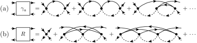
Figure 1: Low-order diagrams for (a) the vertex reducible in antiparallel lines, $\gamma_{a}$, and (b) the totally irreducible vertex $R$. Solid (dashed) lines denote $G^{c}$ ($G^{d}$), and a dot the bare vertex $-U$. The first-order or so-called parquet approximation only retains the bare vertex for $R$.

Diagrams for the four-point vertex are exactly classified by the central parquet equation

$$\Gamma^{(4)}=R+\gamma_{a}+\gamma_{p},\quad I_{a}=R+\gamma_{p},\quad I_{p}=R+\gamma_{a}.$$ (4)

The leading divergence of the XES is determined by only two two-particle channels Roulet et al. (1969); Nozières et al. (1969): $\gamma_{a}$ (cf. Fig. 1(a) ) and $\gamma_{p}$ contain diagrams reducible by cutting two antiparallel or parallel lines, respectively, whereas $I_{a}$ and $I_{p}$ contain diagrams irreducible in the respective channel. The totally irreducible vertex $R$ [cf. Fig. 1(b)] is the only input into the parquet equations, as the reducible vertices are determined self-consistently via Bethe-Salpeter equations [cf. Fig. 2(a)]. Similarly as for the self-energy, terms of $R$ beyond the bare interaction only contribute subleadingly to the XES and can hence be neglected Roulet et al. (1969); Nozières et al. (1969).

In this (parquet) approximation, Eq. (4) together with the Bethe-Salpeter equations for reducible vertices [Fig. 2(a)] form a closed set and can be solved. The analytic solution, employing logarithmic accuracy, provides the leading term of the exponent in Eq. (2). Our numerical solution, to which we compare all following results, is both consistent with the power-law-like behavior of Eq. (2) for small frequencies [cf. Fig. 4(c)] and with the corresponding exponent $\alpha(u)$ [cf. Fig. 4(d)].

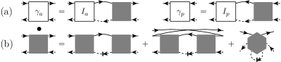
Figure 2: (a) Bethe-Salpeter equations in the antiparallel ($a$) and parallel ($p$) channels. A full square denotes the full vertex $\Gamma^{(4)}$. (b) FRG flow equation for both channls relating $\partial_{\Lambda}\Gamma^{(4)}$ to $\Gamma^{(4)}$ and $\Gamma^{(6)}$. The conventional approximation is to set $\Gamma^{(6)}=0$.

Figure 3: Multiloop fRG flow equations, $\partial_{\Lambda}\gamma_{r}=\sum_{\ell\geq 1}\dot{\gamma}_{r}^{(\ell)}$, for the four-point vertex reducible in channel $r$, with $r=a$ or $p$, and $\bar{r}=p$ or $a$. The subscript $r$ in the diagrams further symbolizes antiparallel or parallel $c$-$d$ lines, respectively. (a) One-loop, (b) two-loop, (c) three- and higher-loop flows. (d) One-loop calculation of $\dot{\gamma}_{r,\textrm{C}}^{(\ell\textrm{\tiny{+}}2)}$, using the previously computed $\dot{\gamma}_{r,\textrm{R}}^{(\ell\textrm{\tiny{+}}1)}$ or $\dot{\gamma}_{r,\textrm{L}}^{(\ell\textrm{\tiny{+}}1)}$.

Multiloop fRG flow.—The functional renormalization group provides an exact flow equation for the four-point vertex as a function of an RG scale parameter $\Lambda$, serving as infrared cutoff. Introducing $\Lambda$ only in the bare $d$ propagator, the flow encompassing both channels Sup is illustrated in Fig. 2(b), where the dashed arrow symbolizes the single-scale propagator $S^{d}_{\Lambda}$. Neglecting self-energies, we have $S^{d}_{\Lambda}=\partial_{\Lambda}G^{d}_{\Lambda}$, and $\partial_{\Lambda}\Gamma^{(4)}$ only depends on $\Gamma^{(4)}$ and $\Gamma^{(6)}$. The boundary conditions $G^{d}_{\Lambda_{i}}=0$ and $G^{d}_{\Lambda_{f}}=G^{d}$ imply $\Gamma^{(4)}_{\Lambda_{i}}=-U$ and $\Gamma^{(6)}_{\Lambda_{i}}=0$.

For almost all purposes, it is unfeasible to treat the six-point vertex exactly. Approximations of $\Gamma^{(6)}$ thus render the fRG flow approximate. The conventional approximation is to set $\Gamma^{(6)}$ and all higher-point vertices to zero, arguing that they are at least of third order in the interaction. This affects the resulting four-point vertex starting at third order and neglects terms that contribute to parquet diagrams Kugler and von Delft . Since, however, the parquet approximation involves only four-point vertices, it should be possible to encode the influence of six- and higher-point vertices during the RG flow by four-point contributions and, still, fully capture all parquet graphs.

In the following, we show how this can be accomplished using mfRG. The first observation is that all the diagrammatic content of the truncated fRG (i.e. without $\Gamma^{(6)}$) is two-particle reducible, due to the bubble structure in the flow equation [first two summands of Fig. 2(b)], very similar to the Bethe-Salpeter equations [Fig. 2(a)]. The only irreducible contribution is the initial condition of the vertex, $\Gamma^{(4)}_{\Lambda_{i}}=-U$. Hence, diagrams generated by the flow are always of the parquet type. It is then natural to express $\Gamma^{(4)}$ as follows, using the channel classification of the parquet equations:

$$\Gamma^{(4)}=-U+\gamma_{a}+\gamma_{p},\qquad\partial_{\Lambda}\gamma_{r}={\textstyle\sum_{\ell\geq 1}}\dot{\gamma}_{r}^{(\ell)}.$$ (5)

Here, $r$ stands for $a$ or $p$ and $\dot{\gamma}_{r}^{(\ell)}$ for diagrams involving $\ell$ loops connecting full vertices. We will show that $\dot{\gamma}_{r}^{(\ell)}$ can be constructed iteratively from lower-loop contributions.

The conventional (or one-loop) fRG flow in channel $r$ is formulated in Fig. 3(a), where full vertices are connected by an $r$ “single-scale” bubble, i.e., either antiparallel or parallel $G^{c}$-$S^{d}$ lines. [Detailed diagrams with all arrows and their mathematical translations are given in Sup , Fig. S2, Eq. (S2).] If one inserts the bare vertex for $\Gamma^{(4)}$ on the r.h.s. of such a one-loop flow equation [Fig. 3(a)], one fully obtains the differentiated second-order vertex. However, inserting first- and second-order vertices on the r.h.s. will miss some diagrams of the differentiated third-order vertex, because these invoke an $\bar{r}$ single-scale bubble that is not generated by $\dot{\gamma}_{r}^{(1)}$ (an overbar denotes the complementary channel: $\bar{a}=p$, $\bar{p}=a$). An example of such a missing third-order diagram is that obtained by differentiating the rightmost $d$ propagator of the third diagram in Fig. 1(a) (cf. Fig. S1 of Sup ). All such neglected contributions can be added to the r.h.s. of the flow equation by hand (replacing bare by full vertices), resulting in the construction in Fig. 3(b). It uses an $r$ “standard” bubble [(anti)parallel $G^{c}$-$G^{d}$ lines] to connect the one-loop contribution from the complementary channel, $\dot{\gamma}_{\bar{r}}^{(1)}$, with the full vertex, thus generating two-loop contributions. These corrections have already been suggested from slightly different approaches Katanin (2004); Eberlein (2014).

The resulting third-order corrected flow will still miss derivatives of parquet graphs starting at fourth order in the interaction. These can be included via two further additions to the flow, which have the same form for all higher loop orders, $\dot{\gamma}_{r}^{(\ell\textrm{\tiny{+}}2)}$ with $\ell\geq 1$ [cf. Fig. 3(c)]. First, for the flow of $\dot{\gamma}_{r}^{(\ell\textrm{\tiny{+}}2)}$, an $r$ bubble is used to attach the previously computed $(\ell+1)$-loop contribution from the complementary channel, $\dot{\gamma}_{\bar{r}}^{(\ell\textrm{\tiny{+}}1)}$, to either side of the full vertex, just as in the two-loop case. Second, by using two $r$ bubbles, we include the differentiated $\ell$-loop vertex from the complementary channel, $\dot{\gamma}_{\bar{r}}^{(\ell)}$, to the flow of $\dot{\gamma}_{r}^{(\ell\textrm{\tiny{+}}2)}$. Double counting of diagrams in all these contributions does not occur due to the unique position of the single-scale propagator Sup . Note that the central term in Fig. 3(c) can be computed by a one-loop integral, too, using the previous computations from the same channel, as shown in Fig. 3(d). Consequently, the numerical effort in the multiloop corrections scales linearly in $\ell$.

By its diagrammatic construction, organized by the number of loops connecting full vertices, the mfRG flow incorporates all differentiated diagrams of a vertex reducible in channel $r$, built up from the bare interaction, and thus captures all parquet graphs of the full four-point vertex. Indeed, in Sup , we prove algebraically for the XES that the number of differentiated diagrams in mfRG matches precisely the number of differentiated parquet graphs. An $\ell$-loop fRG flow generates all parquet diagrams up to order $n=\ell+1$ in the interaction and, naturally, generates an increasing number of parquet contributions at arbitrarily large orders in $U$.

Numerical results—In Fig. 5, we show numerical results for the XES particle-hole susceptibility. Using four different regulators (see below), we compare the susceptibility obtained from an $\ell$-loop fRG flow to the numerical solution of the parquet equations. We find that the one-loop curves differ among each other and deviate strongly from the parquet result. With increasing loop order $\ell$, the multiloop results from all regulators oscillate around and approach the parquet result, with very good agreement already for $\ell=4$. For $\ell\geq 7$, the oscillations in the relative deviation (at $\bar{\omega}=0$) are damped to $\lesssim 2\%$ (insets, solid line). A similar behavior is observed for the identity Wentzell et al. $\Pi_{\bar{\omega}}=\lim_{|\omega|,|\nu|\to\infty}\gamma_{a;\omega,\nu,\bar{\omega}}/U^{2}$ ($\bar{\omega}$ is the exchange frequency, and $\omega$, $\nu$ are two fermionic frequencies), which the parquet solution is guaranteed to fulfill (cf. Ref. Sup, , Eq. (S4) and following) (insets, dashed line).

As regulators, we choose the Litim regulator Litim (2001), and propagators of the type $G^{d}_{\Lambda}(\omega)=\theta(\omega/\Lambda-1)G^{d}(\omega)$, where $\theta(x)$ is either a sharp, smooth, or oscillating step function (cf. Fig. 4(a,b); Eq. (S8) of Sup ). The fact that different regulators give the same result in the mfRG flow is a strong indication for an exact resummation of diagrams.

Let us note that the mfRG flow also increases the stability of the solution towards larger interaction. Whereas, in the one-loop scheme, the four-point vertex diverges for $u>0.4$, higher-loop schemes converge up to larger values of $u$. The reason is that the one-loop scheme contains the full ladder series of diagrams (in any channel), but only parts of nonladder diagrams. Whereas the (imaginary-frequency) pure particle-hole ladder already diverges at $u\sim 0.3$, higher-loop extensions approaching the parquet summation are needed for the full feedback between both channels to eliminate the divergence.

The equivalence between the mfRG flow and parquet summation allows us to explain how the quality of fRG results depends on the choice of regulator. Whereas the one-loop scheme only involves a single-scale bubble $\Pi_{0}^{S}=\sum G^{c}S^{d}$, all extensions invoke successive standard bubbles $\Pi_{0}^{G}=\sum G^{c}G^{d}$. By minimizing the weight of $\Pi_{0}^{G}$ compared to $\Pi_{0}^{S}$, one minimizes the effect of the multiloop corrections and thus the difference between low-level mfRG and parquet. Indeed, from Fig. 4(a,b) we see that a regulator with small (large) weight in $\Pi_{0}^{G}$ and large (small) weight in $\Pi_{0}^{S}$, such as the oscillating-step (Litim) regulator, gives comparatively good (bad) agreement with parquet for low $\ell$. Accordingly, the sharp-step regulator performs slightly better than its smooth counterpart.

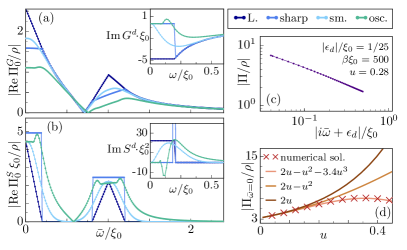
Figure 4: (a) Noninteracting “standard” particle-hole bubble $\Pi_{0}^{G}$ and propagator $G^{d}$ (inset) for different regulators [cf. Eq. (S8) of Ref. Sup, ] and $\Lambda/\xi_{0}=0.2$. (b) Same as (a) for the “single-scale” bubble $\Pi_{0}^{S}$ and propagator $S^{d}$. (c) Double-logarithmic plot for the particle-hole susceptibility $\Pi$, obtained from solving the parquet equations. (d) $\Pi_{\bar{\omega}=0}(u)$ computed via the parquet equations [$\epsilon_{d}$, $\beta$ as in (c)] and according to Eq. (2) with different choices for $\alpha(u)$. The comparison between these guide-to-the-eye lines and the numerical solution confirms that $\alpha(u)\approx 2u$, but also shows that subleading contributions become sizable for larger $u$. These are present since internal numerical calculations go beyond logarithmic accuracy.

Generalizations.—The mfRG flow can be readily extended to more general models, where one normally does not treat two particle species separately, as done here for $c$ and $d$ electrons. If three two-particle channels (antiparallel, parallel, and transverse) are involved, the higher-loop flow must incorporate feedback from both complementary channels via $\dot{\gamma}_{\bar{r}}^{\ell}=\sum_{r^{\prime}\neq r}\dot{\gamma}_{r^{\prime}}^{\ell}$ Kugler and von Delft (2018). The self-energy $\Sigma$ enters the $\Gamma^{(4)}$ flow via full propagators, and, in the one-loop flow of the four-point vertex [Fig. 3(a)], one should follow the usual practice Katanin (2004); Metzner et al. (2012) of using the derivative of the full propagator ($\partial_{\Lambda}G_{\Lambda}$) instead of the single-scale propagator ($S_{\Lambda}=\partial_{\Lambda}G_{\Lambda}|_{\Sigma=\textrm{const.}}$) which excludes any differentiated self-energy contributions. The reason is that, in the exact fRG flow equation [Fig. 2(b)], those diagrams of $\partial_{\Lambda}\Gamma^{(4)}$ that involve $\partial_{\Lambda}\Sigma$ are encoded in the six-point vertex.

Evidently, an improved flow for $\Gamma^{(4)}$ also improves fRG calculations of the self-energy. In the parquet formalism, $\Sigma$ is constructed from the four-point vertex by an exact, self-consistent Schwinger-Dyson equation Bickers (2004). In order to obtain the same self-energy diagrams from the (in principle) exact fRG flow equation for $\Sigma$, with only the vertex in the parquet approximation at one’s disposal, multiloop extensions to the self-energy flow, similar to those introduced here, can be performed Kugler and von Delft (2018). Given the self-energy, all arguments about capturing parquet diagrams (which now consist of dressed lines) with the multiloop fRG flow remain valid since they only involve generic, model-independent statements about the structure of two-particle diagrams.

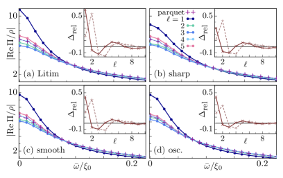
Figure 5: Numerical solutions for the particle-hole susceptibility $\Pi$, obtained from the parquet equations and from mfRG with different regulators [cf. Fig. 4(a,b)], using the parameters of Fig. 4(c). Insets: relative deviation between parquet and mfRG results for $\Pi$ (solid line) and between $\Pi$ and $\lim_{|\omega|,|\nu|\to\infty}\gamma_{a}/U^{2}$ (dashed line), all evaluated at $\bar{\omega}=0$.

The mfRG flow is applicable for any initial condition $\Gamma^{(4)}_{\Lambda_{i}}$. An example where one would not start from $G_{\Lambda_{i}}=0$, as done here, arises in the context of dynamical mean-field theory (DMFT) Georges et al. (1996). There, the goal of adding nonlocal correlations, with the local vertex from DMFT ($\Gamma^{(4)}_{\textrm{DMFT}}$) as input, can be pursued using fRG Taranto et al. (2014). Alternatively, this goal is also being addressed by using the parquet equations in the dynamical vertex approximation (D$\Gamma$A) Toschi et al. (2007); Held et al. (2008); Valli et al. (2010). However, the latter approach requires the diagrammatic decomposition of the nonperturbative vertex $\Gamma^{(4)}_{\textrm{DMFT}}=R+\sum_{r}\gamma_{r}$, which yields diverging results close to a quantum phase transition Schäfer et al. (2013, 2016); *Gunnarsson2017. In contrast, the mfRG flow is built from the full vertex $\Gamma^{(4)}_{\textrm{DMFT}}$ and could thus be used to scan a larger region of the phase diagram.

Conclusion.—Using the X-ray-edge singularity as an example, we have presented multiloop fRG flow equations, which sum up all parquet diagrams to arbitrary order, so that solving the mfRG flow is equivalent to solving the (first-order) parquet equations. Our numerical results demonstrate that solutions of an $\ell$-loop flow quickly approach the parquet result with increasing $\ell$. This applies for a variety of regulators, confirming an exact resummation of diagrams. The mfRG construction is generic and can be readily generalized to more complex models.

The mfRG-parquet equivalence established here shows that one-loop fRG calculations generate only a subset of (differentiated) parquet diagrams and that a multiloop fRG flow is needed to reproduce parquet results. From a practical point of view, mfRG appears advantageous over solving the parquet equations since solving a first-order ordinary differential equation is numerically more stable than solving a self-consistent equation. Moreover, one can choose a suitable regulator and flow from any initial action. Altogether, the mfRG scheme achieves, in effect, a solution of the (first-order) parquet equations while retaining all treasured fRG advantages: no need to solve self-consistent equations, purely one-loop costs, and freedom of choice for regulators.

We thank A. Eberlein, C. Honerkamp, S. Jakobs, V. Meden, W. Metzner, and A. Toschi for useful discussions and acknowledge support by the Cluster of Excellence Nanosystems Initiative Munich. F.B.K. acknowledges funding from the research school IMPRS-QST.

Supplemental material

This supplement consists of four parts. First, we show detailed equations for the mfRG flow, the identity between susceptibility and reducible vertex, and the regulators we used. Second, we provide the numerical details of our computations. Third, we prove algebraically for the XES that the mfRG flow generates all parquet diagrams at arbitrary order, based on expanding the parquet and flow equations in the interaction and counting diagrams. Last, we briefly mention that many quantities appearing in this proof happen to have an interpretation as giving the number of special paths on a triangular grid.

S-I. Detailed equations

Figure S1 illustrates how the two-loop corrections of mfRG cure the flow of the vertex $\gamma_{a}$ at third order in the interaction. Figure S2 shows the detailed form of the mfRG flow equations, corresponding to Fig. 3.

Figure S1 illustrates how the two-loop corrections of mfRG cure the flow of the vertex $\gamma_{a}$ at third order in the interaction. Figure S2 shows the detailed form of the mfRG flow equations from Fig. 3. In principle Sup , the flow equations also contain contributions from a third (transversal) channel, where the interband vertex $\Gamma^{\bar{d}c\bar{c}d}$ is connected to an intraband vertex $\Gamma^{\bar{d}d\bar{d}d}$ by valence band lines $G^{d}$ and $S^{d}$. However, one can easily see that, for the XES, all such terms contribute subleadingly and belong to higher-order diagrams of $R$ in the parquet treatment Roulet et al. (1969). Hence, they are neglected throughout this work.

The mathematical translation of our flow equations only requires the formula for an $r$ bubble connecting two vertices (where $r=a,p$). This is most compactly written in a notation adapted to the respective channel: The three independent frequencies necessary to describe a full vertex can be chosen to include two fermionic frequencies combined with either the bosonic exchange frequency $\bar{\omega}_{a}$, suited for the antiparallel channel, or the bosonic pairing frequency $\bar{\omega}_{p}$, suited for the parallel channel. This is, however, merely a choice of parametrization and does not require any properties of the vertex itself. We choose the parametrization according to $\displaystyle\mathcal{V}_{\omega,\nu,\bar{\omega}_{a}}$ $\displaystyle=\mathcal{V}^{\bar{d}c\bar{c}d}_{\omega,\bar{\omega}_{a}+\omega,\bar{\omega}_{a}+\nu,\nu},$ (S1a) $\displaystyle\mathcal{V}_{\omega,\nu,\bar{\omega}_{p}}$ $\displaystyle=\mathcal{V}^{\bar{d}c\bar{c}d}_{\omega,\bar{\omega}_{p}-\nu,\bar{\omega}_{p}-\omega,\nu},$ (S1b) where the bosonic frequencies are related via $\bar{\omega}_{p}=\bar{\omega}_{a}+\omega+\nu$.

In this notation, an $r$ bubble $\mathcal{V}_{r}$ connecting the vertices $\mathcal{V}^{{}^{\prime}}$ and $\mathcal{V}^{{}^{\prime\prime}}$ can be computed as follows:

$$\mathcal{V}_{r;\omega,\nu,\bar{\omega}_{r}}=\frac{1}{\beta}\sum_{\omega^{\prime}}\mathcal{V}^{{}^{\prime}}_{\omega,\omega^{\prime},\bar{\omega}_{r}}G^{d}_{\omega^{\prime}}G^{c}_{\bar{\omega}_{r}+\sigma_{r}\omega^{\prime}}\mathcal{V}^{{}^{\prime\prime}}_{\omega^{\prime},\nu,\bar{\omega}_{r}},$$ (S2)

with $\sigma_{a}=1$ and $\sigma_{p}=-1$.

The channel notation (S1) is also used in the identity between particle-hole susceptibility $\Pi$ and reducible vertex $\gamma_{a}$ considered in Fig. 5. If we, more generally, denote the susceptibility in the antiparallel channel by $\Pi_{a}=\Pi$ and the one in the parallel channel by $\Pi_{p}$, the relation between susceptibility and 1PI vertex, already used in Eq. (3), reads

$$\Pi_{r;\bar{\omega}_{r}}=\frac{1}{\beta}\sum_{\omega}G^{d}_{\omega}G^{c}_{\bar{\omega}_{r}+\sigma_{r}\omega}\Big{(}1+\frac{1}{\beta}\sum_{\nu}\Gamma^{(4)}_{\omega,\nu,\bar{\omega}_{r}}G^{d}_{\nu}G^{c}_{\bar{\omega}_{r}+\sigma_{r}\nu}\Big{)}.$$ (S3)

The identity between susceptibility and reducible vertex Wentzell et al. is given by

$$\lim_{|\omega|,|\nu|\to\infty}\gamma_{r;\omega,\nu,\bar{\omega}_{r}}=U^{2}\Pi_{r;\bar{\omega}_{r}}.$$ (S4)

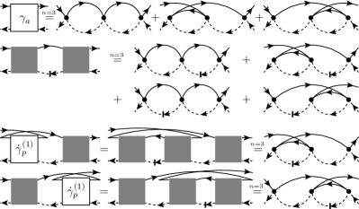
Figure S1: First row: All third-order contributions to $\gamma_{a}$. Its flow is described by the six diagrams obtained by differentiating each dashed line once. In the mfRG scheme, these six diagrams are encoded in $\dot{\gamma}_{a}^{(1)}$ (second and third rows) and $\dot{\gamma}_{a}^{(2)}$ (last two rows), the one- and two-loop flow equations [cf. Fig. S2] for $\gamma_{a}$, respectively. The third-order contributions are obtained by inserting first- and second-order diagrams for the full vertex.

To see that a solution of the parquet equations with any approximation for the totally irreducible vertex $R$ is guaranteed to fulfill Eq. (S4), we note first that, by the very fact that $R$ is totally irreducible, we have

$$\lim_{|\omega|\to\infty}R_{\omega,\nu,\bar{\omega}_{r}}=-U.$$ (S5)

Regarding the reducible vertices, we can perform the limit in the Bethe-Salpeter equations [Fig. 2(a)] and obtain

$$\lim_{|\omega|\to\infty}\gamma_{\bar{r};\omega,\nu,\bar{\omega}_{r}} =0,\quad\Rightarrow\lim_{|\omega|\to\infty}I_{r;\omega,\nu,\bar{\omega}_{r}}=-U,$$ (S6a)

$$\lim_{|\omega|\to\infty}\gamma_{r;\omega,\nu,\bar{\omega}_{r}} =-\frac{U}{\beta}\sum_{\omega^{\prime}}G^{d}_{\omega^{\prime}}G^{c}_{\bar{\omega}_{r}+\sigma_{r}\omega^{\prime}}\Gamma^{(4)}_{\omega^{\prime},\nu,\bar{\omega}_{r}}.$$ (S6b)

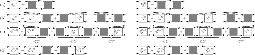
Figure S2: Multiloop flow equations in the (left) antiparallel and (right) parallel channels, corresponding to Fig. 3.

By symmetry [cf. Eq. (S11)], Eqs. (S5), (S6) also hold for $\omega\leftrightarrow\nu$, and we further deduce

$$\lim_{|\nu|\to\infty}\Gamma^{(4)}_{\omega^{\prime},\nu,\bar{\omega}_{r}} =\lim_{|\nu|\to\infty}R_{\omega^{\prime},\nu,\bar{\omega}_{r}}+\lim_{|\nu|\to\infty}\gamma_{r;\omega^{\prime},\nu,\bar{\omega}_{r}}$$

$$=-U-\frac{U}{\beta}\sum_{\omega^{\prime\prime}}\Gamma^{(4)}_{\omega^{\prime},\omega^{\prime\prime},\bar{\omega}_{r}}G^{d}_{\omega^{\prime\prime}}G^{c}_{\bar{\omega}_{r}+\sigma_{r}\omega^{\prime\prime}}.$$ (S7)

Adding the limit $\lim_{|\nu|\to\infty}$ to Eq. (S6b) and using Eqs. (S3) and (S7) yields the identity (S4).

Next, we give the mathematical definition of the regulators, which we have used in the numerical calculations [Fig. 5] and already illustrated in Fig. 4(a,b):

$$G^{d,\textrm{L}}_{\omega,\Lambda} =\frac{1}{i\,\textrm{sgn}(\omega)\,\textrm{max}(|\omega|,\Lambda)-\epsilon_{d}},$$ (S8a)

$$G^{d,\textrm{sharp}}_{\omega,\Lambda} =\Theta(|\omega|-\Lambda)\frac{1}{i\omega-\epsilon_{d}},$$ (S8b)

$$G^{d,\textrm{smooth}}_{\omega,\Lambda} =\bigg{[}1-\,\mathrm{e}^{-\big{(}\frac{|\omega|}{\Lambda}\big{)}^{a}}\bigg{]}\frac{1}{i\omega-\epsilon_{d}},\quad a=2,$$ (S8c)

$$G^{d,\textrm{osc.}}_{\omega,\Lambda} =\,\mathrm{e}^{-\big{(}\frac{\Lambda}{|\omega|}\big{)}^{a}\big{[}1-ib\,\textrm{sgn}(w)\big{]}}\frac{1}{i\omega-\epsilon_{d}},\quad a=2,\ b=1.$$ (S8d)

The regulator in Eq. (S8a) is known as Litim regulator Litim (2001). Note that the parameters in Eqs. (S8c) and (S8d), $$a>0 b G^{d}_{\Lambda_{i}=\infty}=0 G^{d}_{\Lambda_{f}=0}=G^{d}$$ and , can also be chosen differently, keeping the boundary conditions and fulfilled.

Finally, we remark that, in principle, the band gap is the largest energy scale in the XES. This would require $|\epsilon_{d}|\gg\xi_{0}$. However, in the choice of the Hamiltonian [Eq. (1)], we have already restricted ourselves to an interband density-density interaction, which implies individual particle-number conservation. As a consequence, we are free to choose any numerical value for $\epsilon_{d}$, the only exception being $\epsilon_{d}=0$, which violates analytic properties of the (bare) susceptibility Kugler and von Delft . In fact, we find small values for $|\epsilon_{d}|$ most suitable to visualize the power-law divergence in the particle-hole susceptibility for imaginary frequencies [cf. Eq. (2)].

S-II. Numerical details

We have solved the self-consistent parquet equations [Eq. (4), Fig. 2(a)] by an iterative algorithm. For that, we use the initial values $\gamma_{r}=0$ and an update rule that combines the previous value and the predicted value from the Bethe-Salpeter equations according to

$$\gamma_{r}^{\textrm{new}}=z\gamma_{r}^{\textrm{pred.}}+(1-z)\gamma_{r}^{\textrm{prev.}},\quad z\lesssim 0.2.$$ (S9)

The mfRG flow equations are solved by an adaptive-step Runge-Kutta algorithm. The numerical costs of the mfRG flow and the parquet algorithm are similar: In both scenarios, one computes bubbles of vertices multiple times—either to evaluate the flow equations during the mfRG flow or to evaluate the Bethe-Salpeter equations during a self-consistency loop in the parquet algorithm.

In either case, we use a parametrization of four-point vertices which accounts for the important high-frequency asymptotics Li et al. (2016); Wentzell et al. . This parametrization Wentzell et al. is adapted to the channel in which a vertex is reducible: We approximate the frequency dependence of a vertex reducible in channel $r$, using the respective channel notation from Eq. (S1), by

$$\gamma_{r;\omega,\nu,\bar{\omega}_{r}} =\Theta(\Omega_{1}-|\bar{\omega}_{r}|)K^{1}_{\bar{\omega}_{r}}$$ (S10)

$$\ +\Theta(\Omega_{2}-|\bar{\omega}_{r}|)\Theta(\Omega_{2}-|\omega|)K^{2}_{\bar{\omega}_{r},\omega}$$

$$\ +\Theta(\Omega_{2}-|\bar{\omega}_{r}|)\Theta(\Omega_{2}-|\nu|)\bar{K}^{2}_{\bar{\omega}_{r},\nu}$$

$$\ +\Theta(\Omega_{3}-|\bar{\omega}_{r}|)\Theta(\Omega_{3}-|\omega|)\Theta(\Omega_{3}-|\nu|)K^{3}_{\bar{\omega}_{r},\omega,\nu}.$$

Note that the first summand in this parametrization already incorporates the limit used in Eq. (S4). We have chosen the cutoffs $\Omega_{i}$ in Eq. (S10) such that we keep $1000$, $500$, and $100$ positive frequencies on each axis for $K^{1}$, $K^{2}$ and $\bar{K}^{2}$, and $K^{3}$, respectively. Using the symmetries for vertices Wentzell et al. ,

$$(\mathcal{V}_{\omega,\nu,\bar{\omega}_{r}})^{*}=\mathcal{V}_{-\omega,-\nu,-\bar{\omega}_{r}},\quad\mathcal{V}_{\omega,\nu,\bar{\omega}_{r}}=\mathcal{V}_{\nu,\omega,\bar{\omega}_{r}},$$ (S11)

further reduces the computational effort. Note that, while the latter symmetry holds for $\gamma^{(\ell)}_{r}$ and $\gamma^{(\ell)}_{r,\textrm{C}}$, it does not hold for $\gamma^{(\ell)}_{r,\textrm{L}}$ and $\gamma^{(\ell)}_{r,\textrm{R}}$ individually. Instead, one has $\gamma^{(\ell)}_{r,\textrm{L};\omega,\nu,\bar{\omega}_{r}}=\gamma^{(\ell)}_{r,\textrm{R};\nu,\omega,\bar{\omega}_{r}}$.

The Matsubara summations in all our calculations are naturally restricted to a finite frequency interval, since we approximate the $c$ propagator using a sharp cutoff:

$$G^{c}_{\omega} =\rho\int_{-\xi_{0}}^{\xi_{0}}\textrm{d}\epsilon\frac{1}{i\omega-\epsilon}=-2i\rho\arctan\Big{(}\frac{\xi_{0}}{\omega}\Big{)}$$

$$=-i\pi\rho\,\textrm{sgn}(w)\Theta(\xi_{0}-|\omega|)+O\Big{(}\frac{\xi_{0}}{\omega}\Big{)}.$$ (S12)

At an inverse temperature of $\beta\xi_{0}=500$, this yields about $160$ summands.

S-III. Proof of equivalence

We prove below for the XES that solving the full mfRG flow is equivalent to solving the (first-order) parquet equations. We also show that a solution of an $\ell$-loop fRG flow fully contains all parquet graphs up to order $n=\ell+1$. In order to check that the parquet vertex is a solution of the mfRG flow equation (viz., an ordinary differential equation), one has to verify that the initial condition is fulfilled and that the differential equation is fulfilled (during the whole flow). At the initial scale ($\Lambda_{i}=\infty$, $G^{d}_{\Lambda_{i}}=0$, $\Gamma^{(4)}_{\Lambda_{i}}=-U$) the parquet vertex is trivially given by the bare vertex; thus the initial condition is fulfilled. At an arbitrary scale parameter $\Lambda$ during the flow, inserting all parquet diagrams for the vertex into, e.g., the one-loop flow equation generates only a subset of all differentiated parquet diagrams (cf. Fig. S1), i.e., the differential equation is not fulfilled. However, inserting all parquet diagrams into the full mfRG flow equation yields all differentiated parquet diagrams, i.e., the differential equation is fulfilled.

To show that, indeed, all differentiated parquet diagrams are generated in mfRG, we proceeds in two steps: First, we argue that, by the structure of the mfRG flow, the differentiated diagrams are of the parquet type without any double counting. Second, we show (without caring about the specific form of a diagram) that the number of differentiated diagrams in mfRG exactly matches the number of differentiated parquet graphs order for order in the interaction.

.1 No double counting in mfRG

The only totally irreducible contribution to the four-point vertex contained in the multiloop (or conventionally truncated) fRG flow is the bare interaction stemming from the initial condition of the vertex. All further diagrams on the r.h.s. of the flow equations are obtained by iteratively combining two vertices with parallel or antiparallel propagators. Hence, they correspond to differentiated parquet diagrams in the respective channel.

The fact that there is no double counting in mfRG is easily seen employing arguments of diagrammatic reducibility and the unique position of the single-scale propagator in differentiated diagrams. To be specific, let us consider here the channel reducible in antiparallel lines [cf. left side of Fig. S2]; the arguments for the other channel are completely analogous.

First, we note that diagrams in the one-loop term always differ from higher-loop ones. The reason is that, in higher-loop terms, the single-scale propagator appears in the vertex coming from $\partial_{\Lambda}\gamma_{p}$. This can never contain vertices connected by an antiparallel $G^{c}$-$S^{d}$ bubble, since such terms only originate upon differentiating $\gamma_{a}$.

Second, diagrams in the left, center, or right part of an $\ell$-loop contribution always differ. This is because the vertex $\gamma^{(\ell)}_{p}$ is irreducible in antiparallel lines. The left part is then reducible in antiparallel lines only after the single-scale propagator appeared, the right part only before, and the center part is reducible in this channel before and after $S^{d}$.

Third, the same parts (say, the left parts) of different loop contributions ($\ell\neq\ell^{\prime}$) are always different. Assume they agreed: As the antiparallel bubble induces the first (leftmost) reducibility in this channel, already $\gamma^{(\ell)}_{p}$ and $\gamma^{(\ell^{\prime})}_{p}$ would have to agree. For these, only the same parts can agree, as mentioned before. The argument then proceeds iteratively until one compares the one-loop part to a higher-loop ($|\ell-\ell^{\prime}|+1$) one. These are, however, distinct according to the first point.

To summarize: All mfRG diagrams belong to the parquet class and are included at most once. To show that all differentiated parquet diagrams are included, it remains to compare their number to the number of diagrams in mfRG.

.2 Counting the number of diagrams

To count the number of diagrams generated by the parquet equations and mfRG, we expand the parquet (Bethe-Salpeter) and flow equations in the interaction. As we need not consider the specific form of a diagram, the calculation is identical for both channels.

Let us denote the number of parquet diagrams of $\Gamma^{(4)}$ at order $n$ by $P_{0}(n)$ (mnemonic: $P$ for parquet). A $\Gamma^{(4)}$ diagram of order $n$ contains $n-1$ scale-dependent $d$ lines. Differentiating an $n$-th order diagram by $\Lambda$ thus produces $n-1$ differentiated diagrams, and, in total, we have $P_{0}(n)(n-1)$ differentiated diagrams. Let us further denote the number of differentiated diagrams at order $n$ in one channel, generated by mfRG at loop order $\ell$, by $F_{\ell}(n)$ (mnemonic: $F$ for flow). The $\ell$-loop contributions start at order $n=\ell+1$ in the interaction, i.e., $F_{\ell}(n)=0$ for $n\leq\ell$. To show that all parquet diagrams are generated by the (full) mfRG flow, we thus have to establish the following equality:

$$P_{0}(n)(n-1)=2\sum_{\ell=1}^{\infty}F_{\ell}(n)=2\sum_{\ell=1}^{n-1}F_{\ell}(n).$$ (S13)

In order to sum the parquet graphs up to order $n$, it suffices to solve the multiloop fRG flow up to loop order $\ell=n-1$.

First, let us count the number of parquet diagrams. From the Bethe-Salpeter equations [cf. Fig. 2(a)], one can directly deduce the number of diagrams at order $n$ inherent in $\gamma$ (of any channel), $P_{\gamma}(n)$, given the number of diagrams in $I$, $P_{I}$, and in $\Gamma^{(4)}$, $P_{0}$:

$$P_{\gamma}(n)=\sum_{m=1}^{n-1}P_{I}(m)P_{0}(n-m).$$ (S14)

As both $I$ and $\Gamma$ start at order $1$, the order on the l.h.s. exceeds the maximal order of a diagram on the r.h.s. From the parquet equations, we further know

$$P_{0}(1)=1=P_{I}(1);\quad P_{0}(n)=2P_{\gamma}(n)=2P_{I}(n),\,n\geq 2.$$ (S15)

Inserting this, we obtain a closed relation for $P_{0}$:

$$P_{0}(n)=\sum_{m=1}^{n-1}P_{0}(m)P_{0}(n-m)+P_{0}(n-1),\quad n\geq 2.$$ (S16)

Let us solve this recursion by the method of generating functions. We define the generating function $p_{0}(x)$ for the sequence $P_{0}(n)$ by

$$p_{0}(x)=\sum_{n=1}^{\infty}P_{0}(n)x^{n-1}$$ (S17)

and calculate

$$xp_{0}(x)^{2} =x\sum_{n,m=1}^{\infty}P_{0}(n)P_{0}(m)x^{n+m-2}$$

$$=\sum_{n=2}^{\infty}x^{n-1}\sum_{m=1}^{n-1}P_{0}(m)P_{0}(n-m)$$

$$=\sum_{n=2}^{\infty}P_{0}(n)x^{n-1}-\sum_{n=2}^{\infty}P_{0}(n-1)x^{n-1}$$

$$=\sum_{n=1}^{\infty}P_{0}(n)x^{n-1}-1-x\sum_{n=1}^{\infty}P_{0}(n)x^{n-1}.$$ (S18)

From this, we find the defining equation for the generating function,

$$xp_{0}(x)^{2}+(x-1)p_{0}(x)+1=0,$$ (S19)

to which the solution with positive Taylor coefficients is

$$p_{0}(x)=\frac{1-x-\sqrt{1-6x+x^{2}}}{2x}.$$ (S20)

Recognizing that $(1-2tx+x^{2})^{-\lambda}$ is the generating function for Gegenbauer polynomials $C_{n-1}^{\lambda}(t)$ Gradshteyn and Ryzhik (2007), we find

$$P_{0}(n)=-\frac{1}{2}C_{n}^{-1/2}(3),\quad n\geq 2$$ (S21)

and can read off $P_{0}(n)$ from a tabulated sequence:

$$P_{0}:1,\,2,\,6,\,22,\,90,\,394,\,1806,\,8558,\dots$$ (S22)

Note that $P_{0}(n)$ grows exponentially for large $n$. This is much less than the number of all, i.e., parquet and nonparquet diagrams of $\Gamma^{(4)}$, which grows faster than $n!$.

The defining equation for the generating function (S19) can be used to find the generating function $q(x)$ of the related sequence $P_{0}(n)(n-1)$:

$$q(x)=\sum_{n=1}^{\infty}P_{0}(n)(n-1)x^{n-1}=xp^{\prime}_{0}(x).$$ (S23)

Differentiating Eq. (S19), we find the expression

$$0 =p_{0}(x)^{2}+p_{0}(x)+[1-x+2xp_{0}(x)]p^{\prime}_{0}(x),$$

$$\Rightarrow\ q(x) =xp_{0}(x)\frac{p_{0}(x)+1}{1-x-2xp_{0}(x)}.$$ (S24)

Next, we count the number of differentiated diagrams generated by mfRG. For this purpose, we consider the auxiliary vertices in Fig. S3, which can be seen as the building blocks of the multiloop flow equations (Fig. S2). Denoting the number of diagrams of $\dot{\mathcal{V}}_{\ell}$ at order $n$ by $P_{\ell}(n)$, we find, given all parquet diagrams in the full vertex $\Gamma^{(4)}$, similar to Eq. (S14) the relation

$$P_{\ell+1}(n)=\sum_{m=1}^{n-1}P_{\ell}(m)P_{0}(n-m).$$ (S25)

This convolution of two sequences can be expressed in terms of the product of their generating functions, defined by $p_{\ell}(x)=\sum_{n=1}^{\infty}P_{\ell}(n)x^{n-1}$:

$$xp_{\ell}(x)p_{0}(x) =x\sum_{n,m=1}^{\infty}P_{\ell}(n)P_{0}(m)x^{n+m-2}$$

$$=\sum_{n=2}^{\infty}x^{n-1}\sum_{m=1}^{n-1}P_{\ell}(m)P_{0}(n-m)$$

$$=\sum_{n=2}^{\infty}P_{\ell+1}(n)x^{n-1}=p_{\ell+1}(x).$$ (S26)

As a direct consequence, we have

$$p_{\ell}(x)=x^{\ell}p_{0}^{\ell+1}(x);\qquad P_{\ell}(n)=0,\quad\ell\geq n.$$ (S27)

Figure S3: One-loop equations for auxiliary vertices, which can be seen as building blocks for the multiloop flow equations (Fig. S2).

To relate this to mfRG, note that the flow of $n$-th order diagrams is only determined by lower-order diagrams, and that the equivalence (S13) as well as our arguments using generating functions hold for all orders individually. Building the series from the bare interaction, we can therefore assume the parquet diagrams of the vertex on the r.h.s. to be given.

At the one-loop level [Fig. 3(a)], the definitions for $\dot{\gamma}_{a}^{(1)}$ and $\dot{\mathcal{V}}_{1}$ are identical, hence we also have $F_{1}(n)=P_{1}(n)$. For $\dot{\gamma}_{a}^{(2)}$ [Fig. 3(b)], the one-loop contribution from the complementary channel, $\dot{\gamma}_{p}^{(1)}$, is inserted on the left and right side of the full vertex. Both of these parts have the same number of diagrams, which is precisely the number of diagrams in $\dot{\mathcal{V}}_{2}$ (cf. Fig. S3). Hence, we get $F_{2}(n)=2P_{2}(n)$. For all higher loops, $\dot{\gamma}_{a}^{(\ell\textrm{\tiny{+}}2)}$ [Fig. 3(c)], the previous term is similarly inserted on both sides of the full vertex, however the center part is constructed with $\dot{\gamma}_{p}^{(\ell)}$ from loop order $\ell$, and the proportionality relation becomes more complicated. We use an inductive argument, starting at $\ell=3$, and that the number of diagrams contributing to the lower-loop vertices, $\dot{\gamma}_{p}^{(1)}$ and $\dot{\gamma}_{p}^{(2)}$, is obtained by multiplying the number of diagrams of the auxiliary vertices by a counting constant (which keeps track of the different ways to combine vertices at fixed loop order):

$$F_{1}(n)=c_{1}P_{1}(n),\ c_{1}=1;\quad F_{2}(n)=c_{2}P_{2}(n),\ c_{2}=2.$$ (S28)

Using further the equation illustrated in Fig. S4, we similarly obtain for all higher loops:

$$F_{\ell+2}(n)=c_{\ell+2}P_{\ell+2}(n),\quad c_{\ell+2}=2c_{\ell+1}+c_{\ell},\quad\ell\geq 1.$$ (S29)

The recursion relation for $c_{\ell}$ with the initial conditions $c_{1}$ and $c_{2}$ is known to define the so-called Pell numbers (Sloane, , A000129), which are explicitly given by

$$c_{\ell}=\frac{(1+\sqrt{2})^{\ell}-(1-\sqrt{2})^{\ell}}{2\sqrt{2}}.$$ (S30)

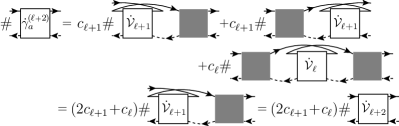
Figure S4: Relation between the number of diagrams contained in $\dot{\gamma}_{a}^{(\ell\textrm{\tiny{+}}2)}$ in $\dot{\mathcal{V}}_{\ell+2}$, where $\#$ symbolizes that we count the number of diagrams of the subsequent vertex.

To summarize, the number of diagrams at order $n$ of the full vertex, generated by mfRG at loop order $\ell$, is given by $2F_{\ell}(n)$, where $F_{\ell}(n)=c_{\ell}P_{\ell}(n)$, with generating functions $f_{\ell}(x)=c_{\ell}p_{\ell}(x)$. Summing all loops, we find by using Eqs. (S27) and (S30):

$$2\sum_{\ell=1}^{\infty}f_{\ell}(x) =\frac{1}{\sqrt{2}}p_{0}(x)\sum_{\sigma=\pm 1}\sigma\sum_{\ell=1}^{\infty}\big{[}xp_{0}(x)(1+\sigma\sqrt{2})\big{]}^{\ell}$$

$$=\frac{1}{\sqrt{2}}p_{0}(x)\sum_{\sigma=\pm 1}\frac{\sigma}{1-xp_{0}(x)(1+\sigma\sqrt{2})}$$

$$=\frac{2xp_{0}(x)^{2}}{1-2xp_{0}(x)-x^{2}p_{0}(x)^{2}}=q(x),$$ (S31)

where the last equality follows by repeated use of Eq. (S19). Consequently, the sequences corresponding to $q(x)$ and $2\sum_{\ell\geq 1}f_{\ell}(x)$ are also equal. Using $F_{\ell}(n)=0$ for $\ell\geq n$ [cf. Eq. (S27)], this means

$$P_{0}(n)(n-1)=2\sum_{\ell=1}^{\infty}F_{\ell}(n)=2\sum_{\ell=1}^{n-1}F_{\ell}(n).$$ (S32)

We thus have shown that the number of differentiated diagrams produced by mfRG at any order $n$ matches the number of differentiated parquet diagrams at this order, and that an $\ell$-loop fRG flow includes all parquet graphs up to order $n=\ell+1$. The details of the proof rely on properties of the XES. However, generalizing the above strategy to more general models should be straightforward.

S-IV. Relation to paths on a triangular grid

As a mathematical curiosity, we mention that the sequences appearing in the previous section have a certain meaning when counting paths on a triangular grid. We are not aware of an underlying connection which goes beyond coincidental properties of the recursion relations of the sequences $P_{\ell}(n)$. Nevertheless, the details are sufficiently intriguing that we present them here.

Figure S5: (a) The (large) Schröder numbers count the number of paths on a triangular grid (in the half-plane) between two points on a line. For $n=4$, these are $22$. $16$ of these have a peak at the first level, $6$ at the second, and only $1$ at the third level [cf. Eq. (S38)]. (b) The Pell numbers count the number of paths on a triangular grid (not restricted to the half-plane) from a point to a vertical line. For $n=3$, these are $5$.

The sequence $P_{0}(n)$ of Eq. (S22), giving the number of parquet graphs at order $n$, happens to be known in the mathematical literature by the name of the (large) Schröder numbers. These denote the number of paths on a half-triangular grid beginning and ending on the horizontal axis (Sloane, , A006318) [cf. Fig. S5(a)]. The sequences $P_{\ell}(n)$ give the number of these paths with a peak at level $\ell$ (Sloane, , A006318-A006321), or the number of paths starting from the left corner and ending at level $\ell$ on the right triangle leg (see below). The Pell numbers [cf. Eq. (S30)] count the number of paths on a triangular grid (not restricted to a half-plane) from a point to a vertical line (Sloane, , A000129)[cf. Fig. S5(b)].

The interpretation for $P_{\ell}(n)$, $\ell\geq 0$, as paths ending on the right triangle leg can be understood from a recursion relation between $P_{\ell}(n)$ with neighboring $\ell$ and $n$ [cf. Eq. (S35)]. For this purpose, let us first derive the relation and construct $P_{\ell}(n)$ as a matrix. By using Eq. (S25) twice and reordering summation indices, we obtain for $\ell,n\geq 1$:

$$P_{\ell+1} (n+1)=\sum_{m=1}^{n}P_{\ell}(m)P_{0}(n+1-m)$$

$$=\sum_{m=1}^{n}\sum_{k=1}^{m-1}P_{\ell-1}(k)P_{0}(m-k)P_{0}(n+1-m)$$

$$=\sum_{m=1}^{n-1}P_{\ell-1}(m)\sum_{k=1}^{n-m}P_{0}(k)P_{0}(n+1-m-k).$$ (S33)

Via Eqs. (S22) and (S25), this yields

$$P_{\ell+1} (n+1)=\sum_{m=1}^{n-1}P_{\ell-1}(m)[P_{0}(n+1-m)-P_{0}(n-m)]$$

$$=\sum_{m=1}^{n-1}P_{\ell-1}(m)P_{0}(n+1-m)-P_{\ell}(n)$$

$$=\sum_{m=1}^{n}P_{\ell-1}(m)P_{0}(n+1-m)-P_{\ell-1}(n)-P_{\ell}(n)$$

$$=P_{\ell}(n+1)-P_{\ell-1}(n)-P_{\ell}(n).$$ (S34)

We can combine this recursion

$$P_{\ell}(n+1)=P_{\ell-1}(n)+P_{\ell}(n)+P_{\ell+1}(n+1)$$ (S35)

with the relation known from Eq. (S16),

$$P_{0}(n+1)=P_{0}(n)+P_{1}(n+1),$$ (S36)

and Eq. (S27), which implies

$$P_{n}(n)=1;\qquad P_{\ell}(n)=0,\quad\ell\geq n.$$ (S37)

These equations suffice to build the following matrix, defined as $A_{n,\ell}=P_{\ell}(n)$, with $n\geq 1$ and $\ell\geq 0$:

$$\bordermatrix{&\!\!\!\!\!\!\!\!\!\!\ell=0,&1,&2,&3,&4,&5,&\dots\cr n=1\,\quad&1&0&\dots&&&&\cr\qquad 2&2&1&0&\dots&&&\cr\qquad 3&6&4&1&0&\dots&&\cr\qquad 4&22&16&6&1&0&\dots&\cr\qquad 5&90&68&30&8&1&0&\dots\cr\qquad\,\vdots&\vdots&&&&&\ddots&\ddots\cr}$$

$$\qquad\qquad\,\,\quad c_{\ell}=1,\,\quad 2,\,\,\quad 5,\,\quad 12,\,\quad 29$$ (S38)

If one distorts the matrix slightly, e.g. by raising the $\ell$-th column by $\ell$ times half the width between subsequent rows and ignores all vanishing entries, one obtains a triangle structure as in Fig. S5. We might consider the entry $A_{0,1}$ as the starting point of paths, for which the steps

$$n\to n+1,\qquad\ell\to\ell,$$ (S39)

$$n\to n+1,\qquad\ell\to\ell+1,$$

$$n\to n,\qquad\ell+1\to\ell$$

are allowed. Then, the entry $A_{n,\ell}$ indeed gives the number of such paths ending at the corresponding point on the triangular grid.

The equality between the number of differentiated parquet and mfRG diagrams shown in Sec. S-III, Eq. (S32), translates into

$$(n-1)A_{n,0}=2\sum_{\ell=1}^{n-1}c_{\ell}A_{n,\ell}.$$ (S40)

While many relations for the matrix $A$ [Eq. (S38)] are known (Sloane, , A033877), we have not found a proof of Eq. (S40) in the literature.

References

- Schäfer et al. (2013) T. Schäfer, G. Rohringer, O. Gunnarsson, S. Ciuchi, G. Sangiovanni, and A. Toschi, Phys. Rev. Lett. 110, 246405 (2013).
- Georges et al. (1996) A. Georges, G. Kotliar, W. Krauth, and M. J. Rozenberg, Rev. Mod. Phys. 68, 13 (1996).
- Rubtsov et al. (2008) A. N. Rubtsov, M. I. Katsnelson, and A. I. Lichtenstein, Phys. Rev. B 77, 033101 (2008).
- Brener et al. (2008) S. Brener, H. Hafermann, A. N. Rubtsov, M. I. Katsnelson, and A. I. Lichtenstein, Phys. Rev. B 77, 195105 (2008).
- Hafermann et al. (2009) H. Hafermann, G. Li, A. N. Rubtsov, M. I. Katsnelson, A. I. Lichtenstein, and H. Monien, Phys. Rev. Lett. 102, 206401 (2009).
- Rohringer et al. (2013) G. Rohringer, A. Toschi, H. Hafermann, K. Held, V. I. Anisimov, and A. A. Katanin, Phys. Rev. B 88, 115112 (2013).
- Ayral and Parcollet (2016) T. Ayral and O. Parcollet, Phys. Rev. B 94, 075159 (2016).
- Toschi et al. (2007) A. Toschi, A. A. Katanin, and K. Held, Phys. Rev. B 75, 045118 (2007).
- Held et al. (2008) K. Held, A. A. Katanin, and A. Toschi, Prog. Theor. Phys. Supp. 176, 117 (2008).
- Valli et al. (2010) A. Valli, G. Sangiovanni, O. Gunnarsson, A. Toschi, and K. Held, Phys. Rev. Lett. 104, 246402 (2010).
- Slezak et al. (2009) C. Slezak, M. Jarrell, T. Maier, and J. Deisz, J. Phys.: Condens. Matter 21, 435604 (2009).
- Metzner et al. (2012) W. Metzner, M. Salmhofer, C. Honerkamp, V. Meden, and K. Schönhammer, Rev. Mod. Phys. 84, 299 (2012).
- Kopietz et al. (2010) P. Kopietz, L. Bartosch, and F. Schütz, Introduction to the Functional Renormalization Group (Lecture Notes in Physics) (Springer, Berlin, 2010).
- Roulet et al. (1969) B. Roulet, J. Gavoret, and P. Nozières, Phys. Rev. 178, 1072 (1969).
- Bickers (2004) N. Bickers, in Theoretical Methods for Strongly Correlated Electrons, CRM Series in Mathematical Physics, edited by D. Sénéchal, A.-M. Tremblay, and C. Bourbonnais (Springer New York, 2004) pp. 237–296.
- Valli et al. (2015) A. Valli, T. Schäfer, P. Thunström, G. Rohringer, S. Andergassen, G. Sangiovanni, K. Held, and A. Toschi, Phys. Rev. B 91, 115115 (2015).
- Li et al. (2016) G. Li, N. Wentzell, P. Pudleiner, P. Thunström, and K. Held, Phys. Rev. B 93, 165103 (2016).
- Gogolin et al. (2004) A. Gogolin, A. Nersesyan, and A. Tsvelik, Bosonization and Strongly Correlated Systems (Cambridge University Press, 2004) p. 332.
- Zanchi and Schulz (2000) D. Zanchi and H. J. Schulz, Phys. Rev. B 61, 13609 (2000).
- Xing et al. (2017) R.-Q. Xing, L. Classen, M. Khodas, and A. V. Chubukov, Phys. Rev. B 95, 085108 (2017).
- Bourbonnais (1991) C. Bourbonnais, in Strongly interacting fermions and high-Tc superconductivity, edited by B. Douçout and J. Zinn-Justin (Elsevier Sience, Amsterdam, 1995, 1991) pp. 307–369.
- Lange et al. (2015) P. Lange, C. Drukier, A. Sharma, and P. Kopietz, J. Phys. A 48, 395001 (2015).
- Nozières et al. (1969) P. Nozières, J. Gavoret, and B. Roulet, Phys. Rev. 178, 1084 (1969).
- Nozières and De Dominicis (1969) P. Nozières and C. T. De Dominicis, Phys. Rev. 178, 1097 (1969).
- Mahan (1967) G. D. Mahan, Phys. Rev. 163, 612 (1967).
- (26) F. B. Kugler and J. von Delft, arXiv:1706.06872 .
- Katanin (2004) A. A. Katanin, Phys. Rev. B 70, 115109 (2004).
- Salmhofer et al. (2004) M. Salmhofer, C. Honerkamp, W. Metzner, and O. Lauscher, Prog. Theor. Phys. 112, 943–970 (2004).
- Eberlein (2014) A. Eberlein, Phys. Rev. B 90, 115125 (2014).
- Giamarchi (2004) T. Giamarchi, Quantum Physics in One Dimension (Clarendon Press, 2004) p. 347.
- Kugler and von Delft (2018) F. B. Kugler and J. von Delft, Phys. Rev. B 97, 035162 (2018).
- (32) See Supplemental Material at http://link.aps.org/ supplemental/10.1103/PhysRevLett.120.057403 for the technical details used in our calculations, which includes Refs. Gradshteyn and Ryzhik, 2007; Sloane, .
- Gradshteyn and Ryzhik (2007) I. Gradshteyn and I. Ryzhik, Table of Integrals, Series, and Products (Seventh Edition), edited by A. Jeffrey and D. Zwillinger (Academic Press, Boston, 2007) p. 990.
- (34) N. J. A. Sloane, The On-Line Encyclopedia of Integer Sequences, (Mar. 2017), published electronically at https://oeis.org.
- Note (1) Since, in a zero-temperature real-frequency treatment Roulet et al. (1969) of X-ray absorption, is purely advanced, we draw diagrams such that all lines are oriented to the left.
- (36) N. Wentzell, G. Li, A. Tagliavini, C. Taranto, G. Rohringer, K. Held, A. Toschi, and S. Andergassen, arXiv:1610.06520 .
- Litim (2001) D. F. Litim, Phys. Rev. D 64, 105007 (2001).
- Taranto et al. (2014) C. Taranto, S. Andergassen, J. Bauer, K. Held, A. Katanin, W. Metzner, G. Rohringer, and A. Toschi, Phys. Rev. Lett. 112, 196402 (2014).
- Note (2) Alternatives to DA which do not require the totally irreducible vertex are the dual fermion Rubtsov et al. (2008); *Brener2008; *Hafermann2009 and the related 1PI approach Rohringer et al. (2013). However, upon transformation to the dual variables, the bare action contains -particle vertices for all . Recent studies Ribic et al. (2017a); *Ribic2017a show that the corresponding six-point vertex yields sizable contributions for the (physical) self-energy, and it remains unclear how a truncation in the (dual) bare action can be justified.
- Ribic et al. (2017a) T. Ribic, G. Rohringer, and K. Held, Phys. Rev. B 95, 155130 (2017a).
- Ribic et al. (2017b) T. Ribic, P. Gunacker, S. Iskakov, M. Wallerberger, G. Rohringer, A. N. Rubtsov, E. Gull, and K. Held, Phys. Rev. B 96, 235127 (2017b).
- Schäfer et al. (2016) T. Schäfer, S. Ciuchi, M. Wallerberger, P. Thunström, O. Gunnarsson, G. Sangiovanni, G. Rohringer, and A. Toschi, Phys. Rev. B 94, 235108 (2016).
- Gunnarsson et al. (2017) O. Gunnarsson, G. Rohringer, T. Schäfer, G. Sangiovanni, and A. Toschi, Phys. Rev. Lett. 119, 056402 (2017).