A deeper view of the CoRoT-9 planetary system

CoRoT-9b is one of the rare long-period ($P=95.3$ days) transiting giant planets with a measured mass known to date. We present a new analysis of the CoRoT-9 system based on five years of radial-velocity (RV) monitoring with HARPS and three new space-based transits observed with CoRoT and Spitzer. Combining our new data with already published measurements we redetermine the CoRoT-9 system parameters and find good agreement with the published values. We uncover a higher significance for the small but non-zero eccentricity of CoRoT-9b ($e=0.133^{+0.042}_{-0.037}$) and find no evidence for additional planets in the system. We use simulations of planet-planet scattering to show that the eccentricity of CoRoT-9b may have been generated by an instability in which a $\sim 50\leavevmode\nobreak\ \hbox{$\mathrm{M}_{\oplus}$}$ planet was ejected from the system. This scattering would not have produced a spin-orbit misalignment, so we predict that the CoRoT-9b orbit should lie within a few degrees of the initial plane of the protoplanetary disk. As a consequence, any significant stellar obliquity would indicate that the disk was primordially tilted.

1 Introduction

As of February 2017, only 27 warm Jupiters (WJs), defined as giant planets ($M_{\rm p}>0.1\leavevmode\nobreak\ \hbox{$\mathrm{M}_{\rm Jup}$}$) with orbital distance $0.1<a<1$ AU (e.g. Dawson & Chiang, 2014), are known to transit in front of their host stars and to have a measured mass better than $3\sigma$. All except four of these WJs were discovered by space-based missions as, in general, only these surveys provide photometric time series of sufficient precision, length, and sampling consistency to detect them. Indeed, the first WJ detected via the transit method was discovered by the CoRoT space telescope; this object, called CoRoT-9b, orbits a non-active G3V star with orbital period $P=95.3$ d and semimajor axis $a=0.41$ AU, and has a mass of $0.84\pm 0.07\leavevmode\nobreak\ \hbox{$\mathrm{M}_{\rm Jup}$}$ and a radius of $1.05\pm 0.04\leavevmode\nobreak\ \hbox{$\mathrm{R}_{\rm Jup}$}$ (Deeg et al., 2010, hereafter D10). Thanks to the Kepler space mission, many more WJ candidates could be found and, for some of them, radial-velocity (RV) follow up (e.g. Santerne et al., 2012, 2016, and references therein) and/or analysis of transit time variations (e.g. Dawson et al., 2012; Borsato et al., 2014; Bruno et al., 2015) have allowed both to unveil their planetary nature and determine their mass and hence their densities. Specifically, 18 of the aforementioned 27 transiting WJs were discovered by Kepler.

The discovery and characterisation of transiting WJs are of great importance to better understand the internal structure, formation, and evolution of giant planets. For instance, the mass-radius relation of giant planets at orbital distances $a>0.1$ AU should not be affected by stellar heating, which is likely related to the inflation mechanism responsible for the large radii of several hot Jupiters (Schneider et al., 2011; Demory & Seager, 2011; Sozzetti et al., 2015). Therefore, WJs are not expected to be inflated unless other processes are at work.

The formation and orbital evolution of WJs is currently a very interesting issue of debate. None of the processes that have been invoked to explain the population of close-in giant exoplanets obviously applies to WJs. Inward type II migration (e.g. Lin et al., 1996) halted by disk photoevaporation may produce WJs (e.g. Alexander & Pascucci, 2012; Mordasini et al., 2012), but this migration cannot explain the high eccentricities of many of them (Bonomo et al., 2017) given that migration in the disk only tends to damp non-zero eccentricities (e.g. Kley & Nelson, 2012). In addition, planet-planet scattering becomes less effective closer to the star (Petrovich et al., 2014). Based on a population-synthesis study, Petrovich & Tremaine (2016) found that $\sim 20\%$ of WJs may have migrated through high-eccentricity migration (e.g. Rasio & Ford, 1996), in particular through the high-eccentricity phase of secular oscillations excited by an outer companion in an eccentric and/or mutually inclined orbit (see also Wu & Lithwick, 2011). On the contrary, Hamers et al. (2017) were not able to produce any WJ from secular evolution in multi-planet systems with three to five giant planets and suggested that WJs either underwent disk migration or formed in situ. In situ formation is proposed by Huang et al. (2016) as the most likely mechanism to form multi-planet systems with WJs flanked by close and smaller companions, such as those observed by Kepler. The rate of occurrence of WJs in such systems may be relatively high, up to $\sim 50\%$, although it is highly uncertain at the moment (Huang et al., 2016). The same authors argued that the WJs without known close companions might represent a distinct population that formed and migrated differently from the former population (e.g. WJs in compact multi-planet systems).

Yet, it is also possible that WJs with no close-in small companions are simply the innermost planetary cores of the system that grew into gas giants and migrated inward. The birth and migration of a gas giant play a crucial role in the evolution and dynamics of a young planetary system. In this context, two aspects can help to explain the lack of (detected) inner companions in these specific systems. The first aspect is that a (forming) gas giant stops the radial flux of small planetesimal and pebbles drifting inward due to gas drag (Lambrechts et al., 2014). This could cause the region inside the orbit of the putative growing and migrating WJ to be too low mass to support, for instance, the formation of any planet larger than the Earth. Secondly, a gas giant formed from the innermost planetary core in the system also acts as an efficient dynamical barrier to additional inward-migrating planetary cores (or planets) formed on outer orbits (Izidoro et al., 2015). Thus, inward-migrating planets from external parts of the disk typically cannot make their full way inward to the innermost regions. They tend to be captured in external mean motion resonances with the gas giant. This could also help to explain the lack of inner companions in these systems. On the other hand, one should naturally expect that outer companions to WJs should be common in this context. However, the subsequent dynamical evolution of these planetary systems post-gas dispersal (e.g. occurrence of dynamical instabilities or not) is determinant in setting the real destiny of these planets.

Monitoring of planetary systems containing WJs that are not flanked by close and small companions, with RV and/or (Gaia) astrometric measurements as well as observations of adaptive optics imaging are crucial to i) search for outer (planetary or stellar) companions; ii) provide information on whether these exterior companions may have triggered high-eccentricity migration (e.g. Bryan et al., 2016); and iii) detect significant orbital eccentricities that could be an imprint of secular chaos or planet-planet scattering possibly occurring after early disk migration (e.g. Marzari et al., 2010).

CoRoT-9b belongs to the class of WJs with no detected close transiting companions. In this work we present photometric follow-up with CoRoT and Spitzer (Sect. 2.1) and spectroscopic monitoring with HARPS for a total time span of almost five years (Sect. 2.2). With a combined Bayesian analysis of photometric and RV data (Sect. 3), we redetermine the system parameters and uncover a higher significance for the small eccentricity of CoRoT-9b (Sect. 4.1). We find no evidence for additional planetary companions in the system with the gathered data (Sect. 4.2). Finally, we investigate several scenarios for the possible formation and migration of CoRoT-9b (Sect. 5.1) and carry out planet-planet scattering simulations to reconstruct the dynamical history of the CoRoT-9 planetary system that best matches the observational constraints (Sect. 5.2).

2 Data

2.1 Photometric data

In addition to one full and one partial transit of CoRoT-9b observed by the CoRoT satellite in 2008 (D10), here we make use of two more transits: the first was observed by Spitzer on 18 June 2010 and the second on 4 July 2011 simultaneously by Spitzer and CoRoT (see Fig. 1). The temporal sampling of CoRoT and Spitzer data is 32 and 31 s, respectively.

CoRoT photometry with the imagette pipeline (e.g. Barros et al. 2014) was obtained during the CoRoT SRc03 pointing, which lasted only five days and was dedicated to the observation of the CoRoT-9b transit. Flux contamination by background stars in the CoRoT mask (Llebaria & Guterman, 2006; Deeg et al., 2009) was estimated to be very low, that is $2.5\%$, by D10 for the data acquired in 2008; we adopted the same value. However, the imagette pipeline does not permit us to estimate such a contamination for the transit observations in 2011 as well; hence we included a dilution factor as an additional free parameter in the transit fitting (Sect. 3).

Both Spitzer observations were secured with the Channel 2 at 4.5 $\mu$m of the IRAC camera (Fazio et al., 2004). These infrared observations and their reduction are described in Lecavelier des Etangs et al. (submitted) who present a search for signatures of rings and satellites around CoRoT-9b. Here we use those Spitzer light curves to refine the parameters of CoRoT-9b and its host star. Briefly, we used the basic calibrated data files of each image as produced by the IRAC pipeline, then corrected them for the so-called pixel-phase effect, which is the oscillation of the measured flux due to the Spitzer jitter and the detector intra-pixel sensitivity variations. Despite this correction, the 2010 Spitzer transit light curve shows two residual systematic effects (Lecavelier des Etangs et al., submitted): first, it presents a “bump” near the middle of the transit, which is unlikely to be due to the crossing of a large starspot by the planet given that the host star is very quiet (no activity features are seen in the CoRoT light curve); secondly, the transit is significantly deeper than that observed in 2011 by $\sim 13\%$ (see Fig. 1 and Sect. 4.1). This larger depth cannot be attributed to unocculted starspots because it would imply a spot filling factor of $\sim 40\%$ that is again unrealistic for the CoRoT-9 low activity level. To overcome these effects, we excluded from our analysis the data points in the bump and, similarly to the 2011 CoRoT transit, we considered a dilution factor for the 2010 Spitzer data to account for its larger depth (see Sect. 3). By doing so, we substantially rely on the 2011 Spitzer transit for the determination of the planetary radius at $4.5\leavevmode\nobreak\ \mu\rm m$ because this transit does not show any feature that might be related to residual systematic effects.

CoRoT and Spitzer transit light curves were normalised following Bonomo et al. (2015); we excluded the partial CoRoT transit for the determination of system parameters (Sect. 3) because of a possible non-optimal normalisation due to the lack of egress data, but we used it for the computation of transit timing variations (TTVs) (Sect. 3 and 4.2). Correlated noise on an hourly timescale in each light curve was estimated as in Aigrain et al. (2009) and Bonomo et al. (2012) but was found to be practically negligible for all the transits. After subtracting the transit model (Sect. 4.1), the CoRoT data have an r.m.s. of $\sim 2.8\cdot 10^{-3}$ in units of relative flux while the Spitzer measurements show a higher r.m.s. of $\sim 4.5\cdot 10^{-3}$; there is no significant difference in the r.m.s. among the CoRoT transits or between the two Spitzer transits.

We also searched for additional transit signals in the CoRoT data with the LAM pipeline (Bonomo et al. 2012; see also Bonomo et al. 2009) after removing the CoRoT-9b transits, but found none (see Sect. 4.2).

2.2 Radial-velocity data

We obtained 28 radial-velocity observations of CoRoT-9 between September 2008 and August 2013 with the HARPS fibre-fed spectrograph (Mayor et al., 2003) at the 3.6 m ESO telescope in La Silla, Chile (programme 184.C-0639). The resolution power is 115,000. Depending on the observations, exposure times range between 40 and 60 min and provide signal-to-noise ratios between 11 and 24 per pixel at 550 nm. All the observations were gathered with the high-accuracy mode (HAM) of HARPS except that at $\rm BJD_{UTC}$=2454766.51, which was secured in high-efficiency (EGGS) mode; we decided to keep this observation in our analysis as it shows no significant drift in radial velocity.

The spectra were extracted using the HARPS pipeline and the radial velocities were measured from the weighted cross-correlation with a numerical mask (Baranne et al., 1996; Pepe et al., 2002). We tested masks representative of F0, G2, and K5 stars. The bluest of the 68 HARPS spectral orders are noisy for that relatively faint ($V=13.7$) star so we adjusted the number of orders used in the cross-correlation. The solution we adopt is the cross-correlation performed with the K5-type mask with the exclusion of the 10 first blue orders. We chose that configuration because it minimises the dispersion of the RV residuals after the Keplerian fit. Other configurations do not provide significantly different system parameters, but their residual dispersions are larger. Following the method presented in Bonomo et al. (2010), moonlight contamination was corrected for 10 observations using the second optical-fibre aperture targeted on the sky. The corrections are of the order of $10\leavevmode\nobreak\ \hbox{\,m\,s${}^{-1}$}$ or less, except for the two most polluted exposures where they are between 25 and $50\leavevmode\nobreak\ \hbox{\,m\,s${}^{-1}$}$.

The RV measurements are reported in Table LABEL:table_rv and shown in Fig. 2. These measurements show variations in phase with the transit ephemeris derived from CoRoT and Spitzer photometry. The bisector spans of the cross-correlation function show neither variations nor trends as a function of radial velocity, confirming that CoRoT-9b is a well-secured planet.

The 28 HARPS measurements we present here have an average precision of $9\hbox{\,m\,s${}^{-1}$}$ and cover a time span of almost five years. This is a significant improvement compared with the 14 measurements gathered by D10 in a one-year time span. The 28 observations presented in Table LABEL:table_rv include those of D10, but with slightly different numerical values as our data reduction is not exactly identical.

Table 1: HARPS radial-velocity measurements of CoRoT-9.

BJDUTC	RV	$\pm$$1\,\sigma$	bisect.†	Texp⋆	S/N⋆⋆
-2 450 000	[ km s-1]	[ km s-1]	[ km s-1]	[sec]
4730.5481	19.785	0.006	-0.003	2700	18.3
4734.5653	19.797	0.008	-0.008	2700	15.7
4739.5092	19.790	0.008	0.022	2700	16.1
4754.5002$\dagger$$\dagger$	19.811	0.011	0.021	3600	19.1
4766.5131	19.838	0.008	-0.001	3600	17.3
4771.5094	19.865	0.014	0.036	3100	10.6
4987.7410$\dagger$$\dagger$	19.802	0.012	0.021	3600	16.0
4993.8179$\dagger$$\dagger$	19.787	0.007	0.000	3600	22.8
5021.6567$\dagger$$\dagger$	19.798	0.009	0.028	3600	19.7
5048.6495$\dagger$$\dagger$	19.850	0.007	0.030	3600	21.8
5063.5679	19.856	0.011	-0.006	3600	16.5
5069.5573	19.849	0.006	0.008	3300	18.7
5077.5704$\dagger$$\dagger$	19.810	0.012	-0.002	3000	16.0
5095.5408	19.789	0.006	0.011	3600	19.7
5341.9076	19.856	0.005	0.002	3600	23.3
5376.7009$\dagger$$\dagger$	19.787	0.014	-0.016	3600	16.5
5400.6811$\dagger$$\dagger$	19.787	0.009	0.030	3600	20.3
5413.6660	19.800	0.005	0.006	3600	24.0
5423.6248	19.833	0.009	-0.026	3600	15.9
5428.5913$\dagger$$\dagger$	19.839	0.015	-0.048	3600	13.7
5658.8885	19.783	0.011	-0.017	3600	13.5
5682.9153	19.779	0.006	0.022	2400	20.9
5713.8266	19.855	0.009	0.026	3600	15.7
5769.5810$\dagger$$\dagger$	19.794	0.009	-0.005	3600	14.9
5824.5177	19.862	0.007	0.004	3600	19.4
6120.6337	19.838	0.011	0.003	3600	12.8
6469.6810	19.807	0.016	0.009	2700	13.9
6515.6036	19.802	0.008	0.006	3600	17.2
$\dagger$: bisector spans; error bars are twice those of the RVs.
$\star$: duration of each individual exposure.
$\star\star$: signal-to-noise ratio per pixel at 550 nm.
$\dagger$$\dagger$: measurements corrected for moonlight pollution.

3 Bayesian data analysis

To derive the system parameters, we carried out a Bayesian combined analysis of the space-based photometric data and ground-based HARPS RVs, using a differential evolution Markov chain Monte Carlo (DE-MCMC) technique (ter Braak, 2006; Eastman et al., 2013). For this purpose, the epochs of the photometric and spectroscopic data were converted into the same unit $\rm BJD_{TDB}$ (Eastman et al., 2010); we used Eq. (4) in Shporer et al. (2014) to perform this correction for the Spitzer data. Given the relatively large semimajor axis of CoRoT-9b, light travel time between the transit measurements and the stellar-centric frame (to which RV epochs are referred) amounts to $\sim 3$ min and was taken into account to have all the data in the same reference frame (the system barycentre).

Our model consists of i) the Keplerian orbit to fit the RVs of the host star and ii) the CoRoT-9b transit model, for which we used the formalism of Mandel & Agol (2002). The free parameters are as follows: the transit epoch $T_{\rm 0}$; the orbital period $P$; the systemic radial velocity $V_{\rm r}$; the radial-velocity semi-amplitude $K$; $\sqrt{e}\leavevmode\nobreak\ {\cos{\omega}}$ and $\sqrt{e}\leavevmode\nobreak\ {\sin{\omega}}$ (e.g. Anderson et al. 2011); a RV jitter term $s_{\rm j}$ added in quadrature to the formal error bars to account for possible extra noise in the RV measurements; the transit duration from first to fourth contact $T_{\rm 14}$; the ratios of the planetary-to-stellar radii $R_{\rm p}/R_{*}$ for both the CoRoT and Spitzer bandpasses; the inclination $i$ between the orbital plane and the plane of the sky; the two limb-darkening coefficients (LDC) $q_{1}=(u_{a}+u_{b})^{2}$ and $q_{2}=0.5u_{a}/(u_{a}+u_{b})$ (Kipping, 2013), where $u_{\rm a}$ and $u_{\rm b}$ are the coefficients of the limb-darkening quadratic law, for both the CoRoT and Spitzer bandpasses; and two contamination factors, one for the CoRoT transit observed in 2011 in imagette mode (see Sect. 2.1) and the other for the Spitzer transit observed in 2010 to account for the significant difference in depth with respect to the 2011 Spitzer transit (Sect. 2.1). Uniform priors were set on all parameters, in particular with bounds of [0, 1] for $q_{1}$ and $q_{2}$ (Kipping, 2013), with a lower limit of zero for $K$ and $s_{\rm j}$, and an upper bound of 1 for the eccentricity; the lower limit of zero simply comes from the choice of fitting $\sqrt{e}\leavevmode\nobreak\ {\cos{\omega}}$ and $\sqrt{e}\leavevmode\nobreak\ {\sin{\omega}}$). Transit fitting was also performed for each individual transit to compute transit timing variations (Sect. 4.2) by fixing $e$ and $\omega$ to the values found with the combined analysis and by imposing a Gaussian prior on transit duration for the partial CoRoT transit.

The DE-MCMC posterior distributions of the model parameters were determined by i) maximising a Gaussian likelihood function (see e.g. Eqs. 9 and 10 in Gregory 2005); ii) adopting the Metropolis-Hastings algorithm to accept or reject the proposed steps; and iii) following the prescriptions given by Eastman et al. (2013) for the employed number of chains (twice the number of free parameters), the removal of burn-in steps, and the criteria for convergence and proper mixing of the chains. As usual, the medians and the $15.86\%$ and $84.14\%$ quantiles of the posterior distributions are taken as the best values and $1\sigma$ uncertainties of the fitted and derived parameters. For parameters consistent with zero, we provide the $1\sigma$ upper limits computed as the $68.27\%$ confidence intervals starting from zero.

The stellar density as derived from the transit fitting, along with the effective temperature and metallicity of CoRoT-9 that are reported in D10, were interpolated to the Yonsei-Yale evolutionary tracks (Demarque et al., 2004) to find the most likely stellar, hence planetary, parameters and their associated uncertainties (e.g. Sozzetti et al., 2007; Bonomo et al., 2014).

4 Results

4.1 System parameters.

Fitted and derived system parameters and their $1\sigma$ error bars are given in Table 2. They are fully consistent, that is within $1\sigma$, with those reported by D10. Figures 1 and 2 show the best-fit models to the full CoRoT and Spitzer transits and the RV data, respectively.

The values of $R_{\rm p}/R_{*}$ in the CoRoT and Spitzer bandpasses agree within $1\sigma$, the former being slightly higher. Flux contamination by background stars in the CoRoT imagette mode was found to be negligible, that is $<0.4\%$; the dilution factor for the first Spitzer transit to account for its larger depth (Sect. 2.1) is $13.2\pm 1.5\%$. The fitted limb-darkening coefficients agree well with the theoretical values computed by Claret & Bloemen (2011) both for the CoRoT and Spitzer bandpasses.

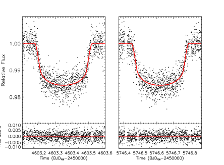
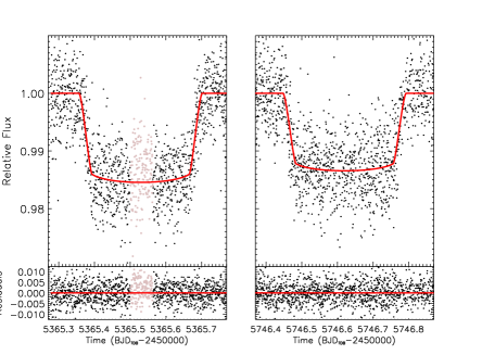
Figure 1: Top panel: CoRoT-9b full transits as observed by the CoRoT satellite with a 32 s cadence (optical band) and the best-fit model (red solid line). Bottom panel: The other two transits observed with Spitzer at $4.5\leavevmode\nobreak\ \rm\mu m$ with a 31 s cadence along with the transit model (red solid line). We note the different transit depths and the “bump” at the middle of the first transit (grey points), which we attribute to uncorrected systematics affecting the 2010 Spitzer transit (see text).

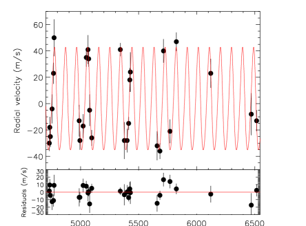
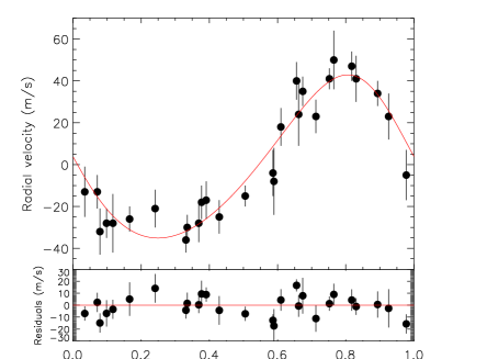
Figure 2: Left panel: HARPS RVs of CoRoT-9 as a function of time and the best Keplerian model (red solid line). Right panel: The same as the left panel but as a function of the orbital phase (transits occur at phase equal to zero/one).

One of the most remarkable results of our analysis is that, by doubling the number of collected HARPS RVs, the significance of the small eccentricity of CoRoT-9b increases from 2.75 (D10) to 3.6$\sigma$, where $e=0.133^{+0.042}_{-0.037}$. To investigate whether the CoRoT-9b small eccentricity is bona fide or might be spurious, we used a Bayesian model comparison to compute the relative probabilities of the eccentric versus circular orbit models by fitting a Keplerian model to the HARPS RVs with Gaussian priors imposed on the photometric transit time and orbital period (Table 2). For this purpose, we computed the Bayesian evidence for both the circular and eccentric models with the Perrakis et al. (2014) method and its implementation as described in Díaz et al. (2016). We found $B_{\rm ecc,circ}=124\pm 8$ in favour of the eccentric model, which means that the eccentric model is $\sim 124$ times more likely than the circular model. According to Kass & Raftery (1995), this value of Bayes factor largely exceeds the threshold ($B=20$) of strong evidence for a more complex model, in our case for the eccentric model with respect to the circular model. This is a significant improvement with respect to the old HARPS data published by D10 because those data only yield $B_{\rm ecc,circ}=4.3\pm 0.4$, which is below the aforementioned threshold to claim a significant eccentricity.

Table 2: CoRoT-9 system parameters.

Stellar parameters
Stellar mass [$\mathrm{M}_{\odot}$]	$0.96\pm 0.04$
Stellar radius [$\mathrm{R}_{\odot}$]	$0.96\pm 0.06$
Stellar density $\rho_{*}$ [$\rm g\;cm^{-3}$]	$1.51\pm 0.30$
Age $t$ [Gyr]	$6\pm 3$
Effective temperature $T_{\rm{eff}}$[K] a	5625 $\pm$ 80
Stellar surface gravity log $g$ [cgs] a	4.54 $\pm$ 0.09
Stellar metallicity $[\rm{Fe/H}]$ [dex] a	-0.01 $\pm$ 0.06
Stellar rotational velocity $V\sin{i_{*}}$ [ km s-1] a	$<3.5$
CoRoT limb-darkening coefficient $q_{1}$	$0.40^{+0.13}_{-0.10}$
CoRoT limb-darkening coefficient $q_{2}$	$0.33^{+0.13}_{-0.10}$
CoRoT limb-darkening coefficient $u_{a}$	$0.41\pm 0.09$
CoRoT limb-darkening coefficient $u_{b}$	$0.22\pm 0.17$
Spitzer limb-darkening coefficient $q_{1}$	$0.035^{+0.037}_{-0.020}$
Spitzer limb-darkening coefficient $q_{2}$	$0.39^{+0.36}_{-0.27}$
Spitzer limb-darkening coefficient $u_{a}$	$0.14^{+0.10}_{-0.08}$
Spitzer limb-darkening coefficient $u_{b}$	$0.037^{+0.14}_{-0.11}$
Systemic velocity $V_{\rm r}$ [ km s-1]	$19.8150\pm 0.0017$
Radial-velocity jitter $s_{\rm j}$ [ m s-1]	$<3.9$
Transit and orbital parameters
Orbital period $P$ [d]	$95.272656\pm 0.000068$
Transit epoch $T_{\rm 0}[\rm BJD_{TDB}-2450000$] b	5365.52723 $\pm$ 0.00037
Transit duration $T_{\rm 14}$ [d]	$0.3445^{+0.0021}_{-0.0018}$
CoRoT bandpass radius ratio $R_{\rm p}/R_{*}$ c	$0.11402_{-0.00085}^{+0.00095}$
Spitzer bandpass radius ratio $R_{\rm p}/R_{*}$ c	$0.11284_{-0.00092}^{+0.00086}$
Inclination $i$ [deg]	$89.900_{-0.084}^{+0.066}$
$a/R_{*}$	$89.9\pm 5.9$
Impact parameter $b$	$0.16^{+0.11}_{-0.09}$
$\sqrt{e}\leavevmode\nobreak\ \cos{\omega}$	$0.29_{-0.08}^{+0.06}$
$\sqrt{e}\leavevmode\nobreak\ \sin{\omega}$	$0.19_{-0.16}^{+0.12}$
Orbital eccentricity $e$	$0.133^{+0.042}_{-0.037}$
Argument of periastron $\omega$ [deg]	$41^{+31}_{-24}$
Radial-velocity semi-amplitude $K$ [ m s-1]	$39.0\pm 2.4$
Planetary parameters
Planet mass $M_{\rm p}\leavevmode\nobreak\ [\hbox{$\mathrm{M}_{\rm Jup}$}]$	$0.84\pm 0.05$
Planet radius $R_{\rm p}\leavevmode\nobreak\ [\hbox{$\mathrm{R}_{\rm Jup}$}]$	$1.066^{+0.075}_{-0.063}$
Planet density $\rho_{\rm p}$ [$\rm g\;cm^{-3}$]	$0.86^{+0.18}_{-0.16}$
Planet surface gravity log $g_{\rm p}$ [cgs]	$3.26\pm 0.06$
Orbital semimajor axis $a$ [AU]	$0.4021\pm 0.0054$
Equilibrium temperature $T_{\rm eq}$ [K] d	$420\pm 16$

4.2 Is CoRoT-9b alone?

As shown in Fig. 2 (lower panels), the residuals of the RVs appear flat, not showing any significant variation attributable to the presence of an additional planetary companion. From these residuals spanning almost five years, we computed the detection limits given the sampling and precision of the HARPS RVs. To this end, we injected into the residuals artificial Keplerian signals of a hypothetical companion by varying its minimum mass and orbital period with logarithmic grids from $1\leavevmode\nobreak\ \hbox{$\mathrm{M}_{\oplus}$}$ to $5\leavevmode\nobreak\ \hbox{$\mathrm{M}_{\rm Jup}$}$ and from 1 d to 5 yr, respectively. For a given minimum mass and orbital period, we generated 500 different realisations of Keplerian models with randomly chosen values of periastron time, argument of periastron, and eccentricity; the maximum allowed eccentricity for each combination of mass and period of the simulated planet was determined from the semi-empirical stability criteria of Giuppone et al. (2013) in the most conservative case, that is by assuming that the orbit of CoRoT-9b and its hypothetical companion are anti-aligned. We carried out simulations by considering only a circular orbit for the second planet as well. Then we made use of both the F-test and the $\chi^{2}$ statistics to exclude planetary companions of a given mass and period that would induce RV variations that are incompatible at $99\%$ confidence level with the observed RV residuals (Fig. 2). In such a way, we derived the upper limits on the minimum mass of a putative second planet as a function of orbital period. These are shown in Fig. 3 for circular (black area) and eccentric (grey contours) orbits. The region around the orbital period of CoRoT-9b is empty because it is dynamically unstable for the planetary minimum masses that are detectable with the gathered HARPS RVs. The peaks at $P\sim 1$ and $2$ yr are due to the temporal sampling of the RV measurements that is inevitably affected by the object’s visibility. From these detection limits, we are able to rule out the presence of massive companions of CoRoT-9b, specifically companions with $M_{\rm p}\sin{i}\gtrsim$0.25, 1.2, and 1.4 $\mathrm{M}_{\rm Jup}$ and $P\sim$10 d, 3 yr, and 5 yr, respectively.

The TTVs show no significant variations from a linear ephemeris either (see Fig. 4 and Table 3). This also suggests the absence of a strong perturber, even though only four transit epochs could be determined.

By considering the r.m.s. of the CoRoT light curve (Sect. 2.1) and $S/N=10$ as the transit detection threshold (Bonomo et al., 2012), we can exclude the presence of inner (coplanar) transiting planets in the system with $R_{\rm p}\gtrsim 1.3$, 2.0, 2.3, and 2.6 $\mathrm{R}_{\oplus}$ and orbital periods $P=1$, 10, 25, and 50 d, respectively.

Table 3: Times of CoRoT-9b mid-transits.

Time	Uncertainty	Instrument
$[\rm BJD_{TDB}-2450000]$	[days]
4603.34577	0.00061	CoRoT
4698.6164	0.0019	CoRoT
5746.61705	0.00074	CoRoT
5365.52764	0.00087	Spitzer
5746.61825	0.00093	Spitzer

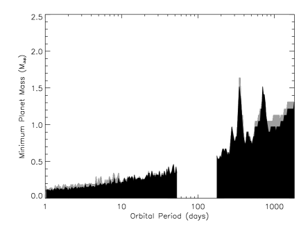
Figure 3: Upper limits on the minimum mass of a possible planetary companion of CoRoT-9b with $99\%$ confidence level as a function of orbital period up to 5 years. Black and shaded areas refer to circular and eccentric orbits of the hypothetical companion; the maximum allowed eccentricity for each period was derived from dynamical stability criteria (see text for more details). The empty region around the orbital period of CoRoT-9b ($P=95.27$ d) is dynamically unstable for the minimum planetary masses detectable with our HARPS RV data.

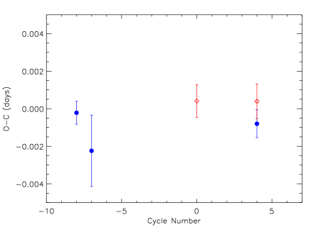
Figure 4: Residuals of the mid-transit epochs of CoRoT-9b vs. the linear ephemeris reported in Table 2. Blue filled circles refer to the transits observed by CoRoT; empty red diamonds indicate the two Spitzer transits. The value with the largest error bar comes from a partial CoRoT transit.

5 Origin of the non-circular orbit of Corot-9b

We now consider the question of the evolution of CoRoT-9b. Given its clearly detected non-zero eccentricity, we place constraints on the dynamical history of the CoRoT-9 system. We first discuss a broad range of potential formation models, culminating with what we consider to be the most likely candidate: planet-planet scattering. Next we present a suite of scattering simulations to reproduce the orbit of CoRoT-9b. Finally, we construct a plausible formation scenario for the system. Our results provide motivation to measure the sky-projected obliquity of the CoRoT-9 system.

5.1 Possible evolutionary scenarios for the CoRoT-9 system

There exist a number of mechanisms that could explain the origin of the CoRoT-9 system.

1. In situ formation of CoRoT-9b from local material at $\sim$0.4 AU. It is possible that there was enough material in the disk for the planet to grow a core of several Earth masses and to accrete gas from the disk (e.g. Ikoma et al., 2001; Hubickyj et al., 2005; Raymond et al., 2008; Batygin et al., 2016). However, if the planet formed in situ, it is hard to understand why only one planet should have formed. And even if there exist additional planets that are too small to detect, why would CoRoT-9b have an eccentric orbit? Additional low-mass planets cannot pump the eccentricity of CoRoT-9b to its observed value. Isolated in situ accretion is implausible.

2. Formation of CoRoT-9b farther from the star followed by gas-driven inward migration. Migration is indeed a likely – and unavoidable – consequence of planet-disk interaction (Goldreich & Tremaine, 1980; Ward, 1986; Lin & Papaloizou, 1986; Papaloizou & Terquem, 2006). Migration is usually directed inward and can plausibly explain the origin of close-in planets of a wide range of masses (Kley & Nelson, 2012; Baruteau et al., 2014). However, simulations show that orbital migration of a single planet universally lowers the orbital eccentricity of a planet (Tanaka & Ward, 2004; Cresswell & Nelson, 2008; Bitsch & Kley, 2010) except in the extreme case of a very massive planet ($M_{\rm p}\sim 5-10\leavevmode\nobreak\ \hbox{$\mathrm{M}_{\rm Jup}$}$) in a very massive disk (Papaloizou et al., 2001; Kley & Dirksen, 2006; Dunhill et al., 2013). The non-zero eccentricity of CoRoT-9b appears to rule out a solitary migration scenario.

3. Inward migration of CoRoT-9b driven by secular forcing from a more distant giant planet. Petrovich & Tremaine (2016) proposed that WJs are driven inward by a combination of secular forcing from a distant companion and tidal dissipation (see also Dawson & Chiang, 2014). In this model, the eccentricity of the inner planet is periodically driven to such high values – and its perihelion distance to such low values – that tidal dissipation shrinks the orbit of the planet. The inner planet is thus driven inward in periodic bursts. However, this model requires the presence of a second planet on a more distant, very eccentric orbit. There is no hint of such a distant perturber (see Sect. 4.2). While constraints on additional planets in the CoRoT-9 system cannot completely rule out this model, it is worth noting that the model struggles to produce WJs with modest ($e\lesssim 0.2$) eccentricities. This scenario appears unlikely to explain the CoRoT-9 system.

4. CoRoT-9b as the survivor of a dynamical instability. The planet-planet scattering model can explain the broad eccentricity distribution of observed giant exoplanets (e.g. Adams & Laughlin, 2003; Chatterjee et al., 2008; Jurić & Tremaine, 2008; Ford & Rasio, 2008; Raymond et al., 2010). This model proposes that the observed planets are the survivors of violent dynamical instabilities in which multiple planets underwent close gravitational encounters. During these gravitational scattering events, one or more planets are lost, usually by ejection into interstellar space (although their numbers are too low to explain the abundance of free-floating gas giants; Veras & Raymond, 2012). The CoRoT-9 system could have formed with one or more additional planets whose orbits became unstable. Given the proximity of CoRoT-9b to the star, the planets may have migrated inward and then become unstable when the gas disk dissipated (see e.g. Ogihara & Ida, 2009; Cossou et al., 2014).

The planet-planet scattering mechanism operates when the gravitational kick of a planet is strong enough that scattering dominates over accretion. This is often quantified with the so-called Safronov number $\Theta$ (Safronov & Zvjagina, 1969), which is defined as the ratio of the escape speed from the surface of a planet to the escape speed from the star, or

$$\Theta^{2}=\left(\frac{GM_{\rm p}}{R_{\rm p}}\right)\left(\frac{a}{GM_{\star}}\right)=\left(\frac{M_{\rm p}}{M_{\star}}\right)\left(\frac{a}{R_{\rm p}}\right),$$ (1)

where $M_{\rm p}$ and $M_{\star}$ are the planetary and stellar masses, respectively, $R_{\rm p}$ is the planet’s radius and $a$ is the orbital radius. Giant exoplanets with larger $\Theta$ are observed to have higher eccentricities (Ford et al., 2001; Ford & Rasio, 2008). For the case of CoRoT-9b, $\Theta=0.66$, that is, close to unity. This puts the planet right at the boundary between the scattering and accretionary regimes. While a scattering origin appears plausible to explain the origin of the non-zero eccentricity of CoRoT-9b, it is worth checking with numerical simulations.

5.2 Scattering simulations to explain the orbit of CoRoT-9b

We ran a suite of numerical simulations of planet-planet scattering. The goal of these simulations was to test whether the orbit of CoRoT-9b can be reproduced by planet scattering. In this context, CoRoT-9b would represent the survivor of a dynamical instability that removed another planet from the system, likely by dynamical ejection. For simplicity we only included one additional planet.

Each simulation contained a star with the properties of CoRoT-9 orbited by two planets: a CoRoT-9b analogue with the actual mass of the planet, and a second planet. CoRoT-9b analogues were initially placed at 0.46 AU on circular orbits. This orbital radius was chosen so that, after ejecting a 50 $M_{\oplus}$ companion, CoRoT-9b would end up on its actual orbit. This initial radius would shift by up to $\sim 0.1$ AU for CoRoT-9b to end up on its actual orbit for the range of extra planet masses considered. While a different initial radius for CoRoT-9b would modestly change its starting Safronov number, this would not affect the outcome of scattering. In fact, we show below that, while changing the Safronov number of CoRoT-9b impacts the branching ratios of different outcomes (i.e. a lower $\Theta^{2}$ implies a higher rate of collisions), it does not change the outcomes themselves (i.e. the final eccentricity of CoRoT-9b is not sensitive to the value of $\Theta^{2}$). The extra planet was placed on an exterior orbit within 2% of the 3:4 or 4:5 mean motion resonances. The reason for this was to remain consistent with a migration origin for the planets, which generally implies resonant capture (e.g. Kley & Nelson, 2012), while being dynamically unstable (Marchal & Bozis, 1982; Gladman, 1993). The orbits of the planets were given a randomly chosen small ($<1^{\circ}$) initial mutual inclination.

We tested two parameters: the mass of the second planet and the physical density of the planets. We considered extra planet masses $M_{\rm extra}=25$, 50, 75, 100, 200 and 267 $\mathrm{M}_{\oplus}$ (the mass of CoRoT-9b is 267 $\mathrm{M}_{\oplus}$). For an extra planet mass of $50\leavevmode\nobreak\ \hbox{$\mathrm{M}_{\oplus}$}$ we also tested physical densities for the planets of 0.5, 1.0, and 2.0 $\rm g\,cm^{-3}$. In all other simulations the densities of both planets were fixed at 1.0 $\rm g\,cm^{-3}$; even though this value is consistent with the measured density of CoRoT-9b within $1\sigma$ ($0.86^{+0.18}_{-0.16}\leavevmode\nobreak\ \rm g\,cm^{-3}$), we show below that the density has no effect on the outcome. For each set we ran 100 simulations.

Each simulation was integrated for 10 million years or until the system became unstable and one planet was removed. We used the Mercury hybrid integrator (Chambers, 1999) with a timestep of 0.1 days. This timestep was small enough to accurately resolve orbits that collided with the star, which were assumed in the calculations to have radii of 0.01 AU (see Appendix A of Raymond et al., 2011, for representative numerical tests). Planets were removed from the system if their orbital radii reached 1000 AU. When this happened, collisions between the planets were treated as inelastic mergers.

Figure 5 shows the orbits of CoRoT-9b analogues at the end of the simulations. The small clump at 0.46 AU represents systems that remained stable; in those cases CoRoT-9b remained on a circular orbit. In simulations in which the two planets collided, CoRoT-9b analogues are at slightly larger orbital radii (0.47-0.52 AU) and with small eccentricities (typically $e\lesssim 0.05$). A collision between CoRoT-9b and an extra planet is clearly inconsistent with the measured eccentricity of CoRoT-9b.

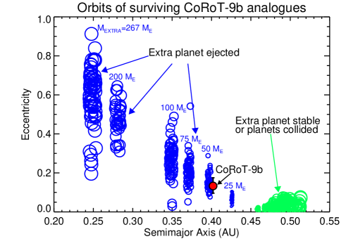
Figure 5: Orbital semimajor axes and eccentricities of surviving CoRoT-9b analogues from our numerical simulations. The blue planets are those that remained after the second planet was ejected; each vertical band corresponds to a specific mass for the extra planet. The green circles are simulations in which either there was no instability or the two planets collided. The measured orbit of CoRoT-9b is shown with the red symbol; the error bars are $1\sigma$.

When the orbits of the planets become unstable and the extra planet is ejected, CoRoT-9b analogues are shifted inward from their initial orbits. The outcomes are radially segregated by the mass of the extra planet because of the mass dependence of the orbital energy exchanged when the extra planet was ejected. In simple terms, CoRoT-9b feels a mass-dependent recoil from ejecting the extra planet. Thus, each vertical “stripe” in Fig. 5 represents the outcome of a set of simulations with a specified extra planet mass. It is important to note that these simulations were designed to reproduce the eccentricity of CoRoT-9b, not its semimajor axis. Thus, even though the simulations with $M_{\rm extra}=50\leavevmode\nobreak\ \hbox{$\mathrm{M}_{\oplus}$}$ are the closest match in semimajor axis, other sets of simulations could easily match the semimajor axis of CoRoT-9b; for example, the simulations with $M_{\rm extra}=75\leavevmode\nobreak\ \hbox{$\mathrm{M}_{\oplus}$}$ would match if CoRoT-9b had started at $\sim$0.49 AU instead of 0.46 AU.

The eccentricities of surviving CoRoT-9b analogues correlate with the mass of the ejected planet. The ejection of a 25 $\mathrm{M}_{\oplus}$ planet only excites CoRoT-9b analogues to an eccentricity of $\sim 0.05,$ whereas ejecting a planet comparable in mass can excite the eccentricities of the planets up to 0.9. Nonetheless, there is a broad range in eccentricities of CoRoT-9b analogues for each set of simulations with a specified extra planet mass. This is because the final eccentricity depends on the details of the last close encounters between the planets, whose alignment is stochastic in nature.

Figure 6 shows the eccentricity of CoRoT-9b analogues after ejecting an extra planet. It is clear that the set of simulations with $M_{\rm extra}=50\leavevmode\nobreak\ \hbox{$\mathrm{M}_{\oplus}$}$ most readily produces CoRoT-9b analogues with the measured eccentricity. However, there is a small tail of outcomes with $M_{\rm extra}=25\leavevmode\nobreak\ \hbox{$\mathrm{M}_{\oplus}$}$ that overlaps with the lower allowed values for CoRoT-9b. At larger masses, a significant fraction of simulations with $M_{\rm extra}=75\leavevmode\nobreak\ \hbox{$\mathrm{M}_{\oplus}$}$ overlap with the higher allowed values, and even some simulations with $M_{\rm extra}=100\leavevmode\nobreak\ \hbox{$\mathrm{M}_{\oplus}$}$ are allowed by observations.

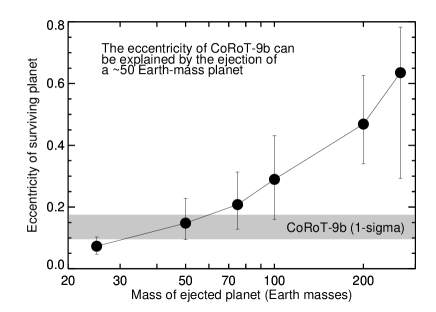
Figure 6: Eccentricity of surviving planets as a function of the mass of the ejected planet. The large points show the median for each set and the error bars show the 5th-95th percentile of outcomes. The shaded area shows the $\pm 1-\sigma$ range of the measured eccentricity of CoRoT-9b.

Planet-planet scattering also excites the planetary orbital inclinations (Jurić & Tremaine, 2008; Chatterjee et al., 2008; Raymond et al., 2010). Indeed, scattering of planets to extremely high eccentricities followed by tidal dissipation has been proposed as a mechanism to produce hot Jupiters whose orbits are misaligned with the stellar equator (Nagasawa et al., 2008; Beaugé & Nesvorný, 2012).

Figure 7 shows the inclinations of surviving CoRoT-9b analogues. None of the planets that match the eccentricity of CoRoT-9b have inclinations larger than $3^{\circ}$. Inclinations above $10^{\circ}$ were only produced in the most energetic scattering events, which also stranded CoRoT-9b analogues on orbits much more eccentric than the real planet.

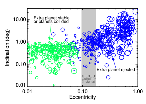
Figure 7: Orbital inclination (zero degrees correspond to the orbital plane prior to scattering phase) vs. eccentricity for CoRoT-9b analogues at the end of our simulations. As in Fig. 5, blue circles represent planets that survived an instability whereas green circles represent planets that either remained on stable orbits or collided with the extra planet (recall that the initial inclination was randomly chosen between zero and $1^{\circ}$). The size of the circle correlates with the mass of the extra planet. The shaded region represents the $1\sigma$ allowed eccentricities for CoRoT-9b.

Our simulations thus predict that the orbit of CoRoT-9b should be in the same plane as it started, to within a few degrees. If we assume that plane to have been aligned with the stellar equator, then this naturally predicts that Rossiter-McLaughlin measurements should find a low stellar obliquity for CoRoT-9, i.e. an alignment between the planetary orbital plane and the stellar equator.

But what would it mean if Rossiter-McLaughlin measurements found a non-zero stellar obliquity? Given the arguments presented above, we think that planet scattering is by far the most likely origin for the eccentric orbit of CoRoT-9b. Assuming that scattering indeed took place, a measured non-zero stellar obliquity would imply that the planetary orbital plane was already misaligned prior to the scattering phase. This would be strong indirect evidence for misalignment of the protoplanetary disk of CoRoT-9. Some candidate mechanisms to tilt disks are chaotic star formation (Bate et al., 2010), magnetic star-disk interactions (Lai et al., 2011), and perturbations from a distant stellar binary (Batygin, 2012; Batygin & Adams, 2013; Lai, 2014). Concerning the latter, even temporary binarity during the embedded cluster phase may tilt the disk.

Finally, we also tested the effect of the planetary density $\rho$ on the outcome of scattering simulations. This could be important because the density is linked to the radius of the planet and therefore its escape speed, and thus the Safronov number $\Theta$.

In the simulations presented above we assumed that both the CoRoT-9b analogues and the extra planet had densities of $\rho=1\leavevmode\nobreak\ \rm g\,cm^{-3}$. We ran three sets of 100 simulations each with $M_{\rm extra}=50\leavevmode\nobreak\ \hbox{$\mathrm{M}_{\oplus}$}$ and varying the density (of both planets) between 0.5 and 2.0 $\rm g\,cm^{-3}$. This corresponded to a range in $\Theta^{2}$ between 0.55 and 0.87. All other aspects of the simulations were as above.

Figure 8 shows the surviving planets in the three sets of simulations with different densities. At a glance the outcomes of the simulations appear similar. Indeed, Kolmogorov-Smirnov tests show that, after ejecting the extra planet, the distribution of eccentricities of CoRoT-9b analogues in all three sets are consistent with having been drawn from the same distribution.

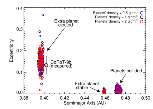
Figure 8: Orbital eccentricity vs. semimajor axis for surviving CoRoT-9b analogues in three sets of simulations that varied the densities of the planets. The blue, black, and red symbols represent simulations in which $\rho=$ 0.5, 1.0, and 2.0 $\rm g\,cm^{-3}$, respectively.

Yet the branching ratios between outcomes did depend on the planet density. In the set of simulations with $\rho=0.5\leavevmode\nobreak\ \rm g\,cm^{-3}$, collisions between the two planets were more than twice as common (53 collisions versus 24) as in the set of simulations with $\rho=2\leavevmode\nobreak\ \rm g\,cm^{-3}$. Ejections were significantly less common in the systems with low-density planets (42 ejections for $\rho=0.5\leavevmode\nobreak\ \rm g\,cm^{-3}$ vs. 67 for $\rho=2.0\leavevmode\nobreak\ \rm g\,cm^{-3}$). The simulations with $\rho=1.0\leavevmode\nobreak\ \rm g\,cm^{-3}$ were intermediate in both cases.

We can conclude from this simple numerical experiment that, while the planet density affects the probability of a given outcome, it has little effect on the details of that outcome.

5.3 A plausible evolutionary history for CoRoT-9b

Given the discussion above and the results of our scattering simulations, we propose the following evolutionary history for the CoRoT-9 system.

• CoRoT-9b formed relatively late in the lifetime of the protoplanetary disk, probably at a few AU, and migrated inward. Its migration stopped at $\sim$0.5 AU because the disk was starting to photo-evaporate (Alexander & Pascucci, 2012).

• A second, $\sim 50\leavevmode\nobreak\ \hbox{$\mathrm{M}_{\oplus}$}$ planet formed in the system. This may have been a second core that formed farther out, migrated inward, and caught up with CoRoT-9b (as in e.g. the Grand Tack model for the Solar System; Walsh et al., 2011), or perhaps a planet whose growth was accelerated by the migration of CoRoT-9b via the “snowplow” effect of migrating resonances (Zhou et al., 2005; Fogg & Nelson, 2005; Raymond et al., 2006; Mandell et al., 2007). The extra planet became locked in (or near; Adams et al., 2008) mean motion resonance with CoRoT-9b.

• The orbits of CoRoT-9b and the extra planet became unstable after the dispersal of the gaseous disk. The two planets scattered off of each other, leading to the ejection of the smaller planet. Nearby small planets were destroyed during the instability (Raymond et al., 2011, 2012). The measured eccentricity of CoRoT-9b is essentially a scar from this instability.

6 Summary and conclusions

Thanks to three new space-based observations of transits of CoRoT-9b with CoRoT and Spitzer and a $\sim$5-yr RV monitoring with HARPS, we updated the CoRoT-9b physical parameters, $M_{\rm p}=0.84\pm 0.05\leavevmode\nobreak\ \hbox{$\mathrm{M}_{\rm Jup}$}$, $R_{\rm p}=1.066^{+0.075}_{-0.063}\leavevmode\nobreak\ \hbox{$\mathrm{R}_{\rm Jup}$}$, and $\rho_{\rm p}=0.86^{+0.18}_{-0.16}\leavevmode\nobreak\ \rm g\;cm^{-3}$, which agree well with the literature values (D10). With the new RV data, we found a higher significance for the non-zero eccentricity $e=0.133^{+0.042}_{-0.037}$ of CoRoT-9b and no evidence for additional companions. The TTVs do not deviate significantly from a linear ephemeris either, thus supporting the absence of a strong perturber, even though only four transit epochs could be determined. Inner transiting (coplanar) planets with $R_{\rm p}\gtrsim 1.3$, 2.0, 2.3, and 2.6 $\mathrm{R}_{\oplus}$ and orbital periods $P=1$, 10, 25, and 50 d, respectively, can be excluded as well using CoRoT data.

We investigated different scenarios to reproduce the orbit of CoRoT-9b, assuming a lack of additional companions. We argue that in situ formation, secular interactions with an outer perturber, and single planet migration are all unlikely to reproduce the CoRoT-9 system. Instead we believe that planet-planet scattering is the most likely origin story for the system.

Using simulations of planet-planet scattering we showed that the eccentricity of CoRoT-9b is likely a residual scar from an instability that ejected a planet of roughly $50\leavevmode\nobreak\ \hbox{$\mathrm{M}_{\oplus}$}$. Although we only performed simulations with a single additional planet, we expect that the same process could have occurred with more planets. The ejection of multiple planets with a total of $\sim 50\leavevmode\nobreak\ \hbox{$\mathrm{M}_{\oplus}$}$ could induce a comparable eccentricity in CoRoT-9b.

Our simulations also serve to motivate future observations of the Rossiter-McLaughlin effect of CoRoT-9b, although challenging given the long transit duration of 8.3 hr (but see e.g. Hébrard et al., 2010, for the case of HD 80606 b). While planet-planet scattering of a $\sim 50\leavevmode\nobreak\ \hbox{$\mathrm{M}_{\oplus}$}$ planet can excite the eccentricity of CoRoT-9b to its current value, there is little associated inclination excitation. The orbital plane of CoRoT-9b should not have changed since before the instability. We thus predict a spin-orbit alignment for the system. Yet perhaps the most interesting outcome would be a measured misalignment, which would be strong indirect evidence that the orbital plane of CoRoT-9b was already misaligned before the instability, perhaps indicating that the protoplanetary disk of the star was tilted at a young age.

References

- Adams & Laughlin (2003) Adams, F. C. & Laughlin, G. 2003, Icarus, 163, 290
- Adams et al. (2008) Adams, F. C., Laughlin, G., & Bloch, A. M. 2008, ApJ, 683, 1117
- Aigrain et al. (2009) Aigrain, S., Pont, F., Fressin, F., et al. 2009, A&A, 506, 425
- Alexander & Pascucci (2012) Alexander, R. D. & Pascucci, I. 2012, MNRAS, 422, 82
- Anderson et al. (2011) Anderson, D. R., Collier Cameron, A., Hellier, C., et al. 2011, ApJ, 726, L19
- Ballerini et al. (2012) Ballerini, P., Micela, G., Lanza, A. F., & Pagano, I. 2012, A&A, 539, A140
- Baranne et al. (1996) Baranne, A., Queloz, D., Mayor, M., et al. 1996, A&AS, 119, 373
- Barros et al. (2014) Barros, S. C. C., Almenara, J. M., Deleuil, M., et al. 2014, A&A, 569, A74
- Baruteau et al. (2014) Baruteau, C., Crida, A., Paardekooper, S.-J., et al. 2014, Protostars and Planets VI, 667
- Bate et al. (2010) Bate, M. R., Lodato, G., & Pringle, J. E. 2010, MNRAS, 401, 1505
- Batygin (2012) Batygin, K. 2012, Nature, 491, 418
- Batygin & Adams (2013) Batygin, K. & Adams, F. C. 2013, ApJ, 778, 169
- Batygin et al. (2016) Batygin, K., Bodenheimer, P. H., & Laughlin, G. P. 2016, ApJ, 829, 114
- Beaugé & Nesvorný (2012) Beaugé, C. & Nesvorný, D. 2012, ApJ, 751, 119
- Bitsch & Kley (2010) Bitsch, B. & Kley, W. 2010, A&A, 523, A30
- Bonomo et al. (2009) Bonomo, A. S., Aigrain, S., Bordé, P., & Lanza, A. F. 2009, A&A, 495, 647
- Bonomo et al. (2012) Bonomo, A. S., Chabaud, P. Y., Deleuil, M., et al. 2012, A&A, 547, A110
- Bonomo et al. (2017) Bonomo, A. S., Desidera, S., Benatti, S., et al. 2017, ArXiv e-prints [arXiv:1704.00373]
- Bonomo et al. (2010) Bonomo, A. S., Santerne, A., Alonso, R., et al. 2010, A&A, 520, A65
- Bonomo et al. (2014) Bonomo, A. S., Sozzetti, A., Lovis, C., et al. 2014, A&A, 572, A2
- Bonomo et al. (2015) Bonomo, A. S., Sozzetti, A., Santerne, A., et al. 2015, A&A, 575, A85
- Borsato et al. (2014) Borsato, L., Marzari, F., Nascimbeni, V., et al. 2014, A&A, 571, A38
- Bruno et al. (2015) Bruno, G., Almenara, J.-M., Barros, S. C. C., et al. 2015, A&A, 573, A124
- Bryan et al. (2016) Bryan, M. L., Knutson, H. A., Howard, A. W., et al. 2016, ApJ, 821, 89
- Chambers (1999) Chambers, J. E. 1999, MNRAS, 304, 793
- Chatterjee et al. (2008) Chatterjee, S., Ford, E. B., Matsumura, S., & Rasio, F. A. 2008, ApJ, 686, 580
- Claret & Bloemen (2011) Claret, A. & Bloemen, S. 2011, A&A, 529, A75
- Cossou et al. (2014) Cossou, C., Raymond, S. N., Hersant, F., & Pierens, A. 2014, A&A, 569, A56
- Cresswell & Nelson (2008) Cresswell, P. & Nelson, R. P. 2008, A&A, 482, 677
- Dawson & Chiang (2014) Dawson, R. I. & Chiang, E. 2014, Science, 346, 212
- Dawson et al. (2012) Dawson, R. I., Johnson, J. A., Morton, T. D., et al. 2012, ApJ, 761, 163
- Deeg et al. (2009) Deeg, H. J., Gillon, M., Shporer, A., et al. 2009, A&A, 506, 343
- Deeg et al. (2010) Deeg, H. J., Moutou, C., Erikson, A., et al. 2010, Nature, 464, 384
- Demarque et al. (2004) Demarque, P., Woo, J.-H., Kim, Y.-C., & Yi, S. K. 2004, ApJS, 155, 667
- Demory & Seager (2011) Demory, B.-O. & Seager, S. 2011, ApJS, 197, 12
- Díaz et al. (2016) Díaz, R. F., Ségransan, D., Udry, S., et al. 2016, A&A, 585, A134
- Dunhill et al. (2013) Dunhill, A. C., Alexander, R. D., & Armitage, P. J. 2013, MNRAS, 428, 3072
- Eastman et al. (2013) Eastman, J., Gaudi, B. S., & Agol, E. 2013, PASP, 125, 83
- Eastman et al. (2010) Eastman, J., Siverd, R., & Gaudi, B. S. 2010, PASP, 122, 935
- Fazio et al. (2004) Fazio, G. G., Hora, J. L., Allen, L. E., et al. 2004, ApJS, 154, 10
- Fogg & Nelson (2005) Fogg, M. J. & Nelson, R. P. 2005, A&A, 441, 791
- Ford et al. (2001) Ford, E. B., Havlickova, M., & Rasio, F. A. 2001, Icarus, 150, 303
- Ford & Rasio (2008) Ford, E. B. & Rasio, F. A. 2008, ApJ, 686, 621
- Giuppone et al. (2013) Giuppone, C. A., Morais, M. H. M., & Correia, A. C. M. 2013, MNRAS, 436, 3547
- Gladman (1993) Gladman, B. 1993, Icarus, 106, 247
- Goldreich & Tremaine (1980) Goldreich, P. & Tremaine, S. 1980, ApJ, 241, 425
- Gregory (2005) Gregory, P. C. 2005, ApJ, 631, 1198
- Hamers et al. (2017) Hamers, A. S., Antonini, F., Lithwick, Y., Perets, H. B., & Portegies Zwart, S. F. 2017, MNRAS, 464, 688
- Hébrard et al. (2010) Hébrard, G., Désert, J.-M., Díaz, R. F., et al. 2010, A&A, 516, A95
- Huang et al. (2016) Huang, C., Wu, Y., & Triaud, A. H. M. J. 2016, ApJ, 825, 98
- Hubickyj et al. (2005) Hubickyj, O., Bodenheimer, P., & Lissauer, J. J. 2005, Icarus, 179, 415
- Ikoma et al. (2001) Ikoma, M., Emori, H., & Nakazawa, K. 2001, ApJ, 553, 999
- Izidoro et al. (2015) Izidoro, A., Raymond, S. N., Morbidelli, A., Hersant, F., & Pierens, A. 2015, ApJ, 800, L22
- Jurić & Tremaine (2008) Jurić, M. & Tremaine, S. 2008, ApJ, 686, 603
- Kass & Raftery (1995) Kass, R. E. & Raftery, A. E. 1995, Journal of the American Statistical Association, 90, 773
- Kipping (2013) Kipping, D. M. 2013, MNRAS, 435, 2152
- Kley & Dirksen (2006) Kley, W. & Dirksen, G. 2006, A&A, 447, 369
- Kley & Nelson (2012) Kley, W. & Nelson, R. P. 2012, ARA&A, 50, 211
- Lai (2014) Lai, D. 2014, MNRAS, 440, 3532
- Lai et al. (2011) Lai, D., Foucart, F., & Lin, D. N. C. 2011, MNRAS, 412, 2790
- Lambrechts et al. (2014) Lambrechts, M., Johansen, A., & Morbidelli, A. 2014, A&A, 572, A35
- Lecavelier des Etangs et al. ( submitted) Lecavelier des Etangs, A., Hébrard, G., Blandin, S., et al. submitted, A&A
- Lin et al. (1996) Lin, D. N. C., Bodenheimer, P., & Richardson, D. C. 1996, Nature, 380, 606
- Lin & Papaloizou (1986) Lin, D. N. C. & Papaloizou, J. 1986, ApJ, 309, 846
- Llebaria & Guterman (2006) Llebaria, A. & Guterman, P. 2006, in ESA Special Publication, Vol. 1306, The CoRoT Mission Pre-Launch Status - Stellar Seismology and Planet Finding, ed. M. Fridlund, A. Baglin, J. Lochard, & L. Conroy, 293
- Mandel & Agol (2002) Mandel, K. & Agol, E. 2002, ApJ, 580, L171
- Mandell et al. (2007) Mandell, A. M., Raymond, S. N., & Sigurdsson, S. 2007, ApJ, 660, 823
- Marchal & Bozis (1982) Marchal, C. & Bozis, G. 1982, Celestial Mechanics, 26, 311
- Marzari et al. (2010) Marzari, F., Baruteau, C., & Scholl, H. 2010, A&A, 514, L4
- Mayor et al. (2003) Mayor, M., Pepe, F., Queloz, D., et al. 2003, The Messenger, 114, 20
- Mordasini et al. (2012) Mordasini, C., Alibert, Y., Benz, W., Klahr, H., & Henning, T. 2012, A&A, 541, A97
- Nagasawa et al. (2008) Nagasawa, M., Ida, S., & Bessho, T. 2008, ApJ, 678, 498
- Ogihara & Ida (2009) Ogihara, M. & Ida, S. 2009, ApJ, 699, 824
- Papaloizou et al. (2001) Papaloizou, J. C. B., Nelson, R. P., & Masset, F. 2001, A&A, 366, 263
- Papaloizou & Terquem (2006) Papaloizou, J. C. B. & Terquem, C. 2006, Reports on Progress in Physics, 69, 119
- Pepe et al. (2002) Pepe, F., Mayor, M., Galland, F., et al. 2002, A&A, 388, 632
- Perrakis et al. (2014) Perrakis, K., Ntzoufras, I., & Tsionas, E. G. 2014, Computational Statistics & Data Analysis, 77, 54
- Petrovich & Tremaine (2016) Petrovich, C. & Tremaine, S. 2016, ApJ, 829, 132
- Petrovich et al. (2014) Petrovich, C., Tremaine, S., & Rafikov, R. 2014, ApJ, 786, 101
- Rasio & Ford (1996) Rasio, F. A. & Ford, E. B. 1996, Science, 274, 954
- Raymond et al. (2010) Raymond, S. N., Armitage, P. J., & Gorelick, N. 2010, ApJ, 711, 772
- Raymond et al. (2011) Raymond, S. N., Armitage, P. J., Moro-Martín, A., et al. 2011, A&A, 530, A62
- Raymond et al. (2012) Raymond, S. N., Armitage, P. J., Moro-Martín, A., et al. 2012, A&A, 541, A11
- Raymond et al. (2008) Raymond, S. N., Barnes, R., & Mandell, A. M. 2008, MNRAS, 384, 663
- Raymond et al. (2006) Raymond, S. N., Mandell, A. M., & Sigurdsson, S. 2006, Science, 313, 1413
- Safronov & Zvjagina (1969) Safronov, V. S. & Zvjagina, E. V. 1969, Icarus, 10, 109
- Santerne et al. (2012) Santerne, A., Díaz, R. F., Moutou, C., et al. 2012, A&A, 545, A76
- Santerne et al. (2016) Santerne, A., Moutou, C., Tsantaki, M., et al. 2016, A&A, 587, A64
- Schneider et al. (2011) Schneider, J., Dedieu, C., Le Sidaner, P., Savalle, R., & Zolotukhin, I. 2011, A&A, 532, A79
- Shporer et al. (2014) Shporer, A., O’Rourke, J. G., Knutson, H. A., et al. 2014, ApJ, 788, 92
- Sozzetti et al. (2015) Sozzetti, A., Bonomo, A. S., Biazzo, K., et al. 2015, A&A, 575, L15
- Sozzetti et al. (2007) Sozzetti, A., Torres, G., Charbonneau, D., et al. 2007, ApJ, 664, 1190
- Tanaka & Ward (2004) Tanaka, H. & Ward, W. R. 2004, ApJ, 602, 388
- ter Braak (2006) ter Braak, C. J. F. 2006, Statistics and Computing, 16, 239
- Veras & Raymond (2012) Veras, D. & Raymond, S. N. 2012, MNRAS, 421, L117
- Walsh et al. (2011) Walsh, K. J., Morbidelli, A., Raymond, S. N., O’Brien, D. P., & Mandell, A. M. 2011, Nature, 475, 206
- Ward (1986) Ward, W. R. 1986, Icarus, 67, 164
- Wu & Lithwick (2011) Wu, Y. & Lithwick, Y. 2011, ApJ, 735, 109
- Zhou et al. (2005) Zhou, J.-L., Aarseth, S. J., Lin, D. N. C., & Nagasawa, M. 2005, ApJ, 631, L85