On the choice of beam polarization in $e^{+}e^{-}\to ZZ/Z\gamma$ and anomalous triple gauge-boson couplings

Abstract

The anomalous trilinear gauge couplings of $Z$ and $\gamma$ are studied in $e^{+}e^{-}\to ZZ/Z\gamma$ with longitudinal beam polarizations using a complete set of polarization asymmetries for the $Z$ boson. We quantify the goodness of the beam polarization in terms of the likelihood and find the best-choice of $e^{-}$ and $e^{+}$ polarizations to be ($+0.16$, $-0.16$), ($+0.09$, $-0.10$) and ($+0.12$, $-0.12$) for $ZZ$, $Z\gamma$ and combined processes, respectively. Simultaneous limits on anomalous couplings are obtained for these choices of beam polarizations using Markov-Chain–Monte-Carlo (MCMC) for an $e^{+}e^{-}$ collider running at $\sqrt{s}=500$ GeV and $\mathcal{L}=100$ fb^-1. We find the simultaneous limits for these beam polarizations to be comparable with each other and also comparable with the unpolarized beam case.

1 Introduction

The gauge boson sector in the Standard Model (SM) remains uncharted even after the discovery of Higgs boson Chatrchyan:2012xdj at LHC. Of the gauge-boson self couplings (trilinear and quartic), the gauge boson couplings to Higgs, the Higgs self couplings, which are the key to understand Electro Weak Symmetry Breaking (EWSB), there have no precise measurements and they need serious attention. The future International Linear Collider (ILC) Djouadi:2007ik ; Baer:2013cma ; Behnke:2013xla will be a precision testing machine MoortgatPick:2005cw which will have the possibility of polarized initial beams. Two types of polarization, namely longitudinal and transverse, for both initial beams ($e^{-}$ and $e^{+}$) will play an important role in precise measurement of various parameters, like the coupling among gauge bosons, Higgs coupling to the top quark, and Higgs coupling to the gauge boson. Beam polarization has the ability to enhance the relevant signal to background ratio along with the sensitivity of observables MoortgatPick:2005cw ; Andreev:2012cj ; Ananthanarayan:2010bt ; Osland:2009dp ; Pankov:2005kd . It can also be used to separate CP-violating couplings from a CP-conversing one MoortgatPick:2005cw ; Kittel:2011rk ; Dreiner:2010ib ; Bartl:2007qy ; Rao:2006hn ; Bartl:2005uh ; Czyz:1988yt ; Choudhury:1994nt ; Ananthanarayan:2004eb ; Ananthanarayan:2011fr ; Ananthanarayan:2003wi if CP-violation is present in Nature. These potentials of the beam polarizations have been explored, for example, to study $\tau$ polarization Dreiner:2010ib , top quark polarization Groote:2010zf and its anomalous couplings Amjad:2015mma , littlest Higgs model Ananthanarayan:2009dw , $WWV$ couplings Ananthanarayan:2011ga ; Andreev:2012cj ; Ananthanarayan:2010bt , Higgs couplings to gauge bosons Kumar:2015eea ; Rindani:2010pi ; Biswal:2009ar ; Rindani:2009pb .

Here we use beam polarizations (longitudinal only) to study anomalous trilinear gauge-boson self couplings in the neutral sector using the complete set of polarization observables of the $Z$ boson Rahaman:2016pqj ; Boudjema:2009fz ; Aguilar-Saavedra:2015yza in the process $e^{+}e^{-}\to ZZ/Z\gamma$. The anomalous couplings among the neutral gauge boson have been studied earlier with unpolarized beam in Boudjema:92 ; Baur:1992cd ; Ellison:1998uy ; Baur:2000ae ; Ananthanarayan:2005ib ; Aihara:1995iq ; Gounaris:2000dn ; Poulose:1998sd ; Senol:2013ym as well as with polarized beams in Ots:2006dv ; Czyz:1988yt ; Choudhury:1994nt ; Ananthanarayan:2004eb ; Ananthanarayan:2014sea ; Gounaris:1999kf ; Choi:1994nv ; Rizzo:1999xj ; Atag:2003wm ; Ananthanarayan:2003wi . Some of these studies have used given beam polarizations to enhance the sensitivity of observables, while others have used two different sets of beam polarizations to construct the observables. We follow the former method and quantify the likelihood-based goodness of the choice of beam polarizations.

For the process of interest the anomalous triple gauge-boson couplings is given by the Lagrangian Gounaris:1999kf ; Rahaman:2016pqj

$${\cal L}=\frac{g_{e}}{M_{Z}^{2}}\Bigg{[}[f_{4}^{Z}(\partial_{\mu}Z^{\mu\beta})-f_{4}^{\gamma}(\partial_{\mu}F^{\mu\beta})]Z_{\alpha}(\partial^{\alpha}Z_{\beta})$$

$$+[f_{5}^{\gamma}(\partial^{\sigma}F_{\sigma\mu})+f_{5}^{Z}(\partial^{\sigma}Z_{\sigma\mu})]\widetilde{Z}^{\mu\beta}Z_{\beta}$$

$$-[h_{1}^{\gamma}(\partial^{\sigma}F_{\sigma\mu})+h_{1}^{Z}(\partial^{\sigma}Z_{\sigma\mu})]Z_{\beta}F^{\mu\beta}$$

$$-[h_{3}^{\gamma}(\partial_{\sigma}F^{\sigma\rho})+h_{3}^{Z}(\partial_{\sigma}Z^{\sigma\rho})]Z^{\alpha}\widetilde{F}_{\rho\alpha}\Bigg{]}.$$ (1)

The coupling $f_{i}^{V}$s appear in the $ZZ$ process while $h_{i}^{V}$s appear in $Z\gamma$ process. Among these couplings $f_{4}^{V}$ and $h_{1}^{V}$ are $CP$-odd while others are $CP$-even. The best limits on these anomalous couplings coming from LHC are $|f_{i}^{V}|\sim 3\times 10^{-3}$ Khachatryan:2015pba and $|h_{i}^{V}|\sim 9\times 10^{-4}$ Aad:2016sau .

The rest of the paper is organized as follows. In section 2 we discuss basic formulations and the $Z$ boson polarization observables. In section 3 we study beam polarization dependence of sensitivity and likelihood. We define a measure of goodness for the choice of beam polarizations and study $ZZ/Z\gamma$ processes to obtain the best choices. The simultaneous limits are presented for a set of beam polarizations. We conclude in section 4.

2 Beam polarization and polarization observables

The polarization density matrices for $e^{-}$ and $e^{+}$ beams are given by

$$P_{e^{-}}(\lambda_{e^{-}},\lambda_{e^{-}}^{\prime})=\frac{1}{2}\left[\begin{tabular}[]{cc}$(1+\eta_{3})$&$\eta_{T}$\\ $\eta_{T}$&$(1-\eta_{3})$\end{tabular}\right]\hskip 14.22636pt\textrm{and}$$ (4)

$$P_{e^{+}}(\lambda_{e^{+}},\lambda_{e^{+}}^{\prime})=\frac{1}{2}\left[\begin{tabular}[]{cc}$(1+\xi_{3})$&$\xi_{T}e^{-i\delta}$\\ $\xi_{T}e^{i\delta}$&$(1-\xi_{3})$\end{tabular}\right],$$ (7)

where $\eta_{3}$ and $\eta_{T}$ ($\xi_{3}$ and $\xi_{T}$) are longitudinal and transverse polarization of $e^{-}$ ($e^{+}$) with $\delta$ being the azimuthal angle between two transverse polarizations. The positive $x$-axis is taken along the transverse polarization of $e^{-}$ and positive $z$-axis along its momentum.

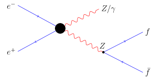
Figure 1: Feynman diagram for production of $Z$ boson and its decay to a pair of fermions

The density matrix for the production of $Z$ boson in the above process (Fig. 1 ) would be

$$\rho(\lambda_{Z},\lambda_{Z}^{\prime})={\cal\>\sum}_{\lambda_{e^{-}},\lambda_{e^{-}}^{\prime},\lambda_{e^{+}},\lambda_{e^{+}}^{\prime}}{\cal M}^{\dagger}(\lambda_{e^{-}}^{\prime},\lambda_{e^{+}}^{\prime},\lambda_{Z}^{\prime})\times$$

$${\cal M}(\lambda_{e^{-}},\lambda_{e^{+}},\lambda_{Z})\times P_{e^{-}}(\lambda_{e^{-}},\lambda_{e^{-}}^{\prime})\times P_{e^{+}}(\lambda_{e^{+}},\lambda_{e^{+}}^{\prime}).$$ (8)

We note that the different helicities can take the following values:

$$\lambda_{Z},\lambda_{Z}^{\prime}\in\{-1,0,1\}\ \text{and}\ \lambda_{e^{\pm}},\lambda_{e^{\pm}}^{\prime}\in\{-1,1\}.$$ (9)

For the present work we restrict ourselves only to the longitudinal beam polarizations, i.e. $\eta_{T}=0=\xi_{T}$. With the chosen beam polarizations we construct the complete set of eight polarization observables for the $Z$ boson along with total cross section in the processes $e^{+}e^{-}\to ZZ/Z\gamma$. These polarization observables can be obtained analytically from the production process as well as from asymmetries constructed from decay distribution of the particle. The polarization observables consist of a $3$ component vector polarization $\vec{P}\equiv(P_{x},P_{y},P_{z})$ and a traceless symmetric rank-$2$ tensor $T_{ij}(i,j=x,y,z)$ with $5$ independent component $T_{xy}$, $T_{xz}$, $T_{yz}$, $T_{xx}-T_{yy}$ and $T_{zz}$. The asymmetries in the collider or in a Monte Carlo event generator corresponding to $P_{i}$’s and $T_{ij}$’s are $\{A_{x},A_{y},A_{z}\}$ and $\{A_{xy},A_{xz},A_{yz},A_{x^{2}-y^{2}},A_{zz}\}$, respectively. The asymmetries $A_{z}$, $A_{xz}$, $A_{yz}$ are zero in SM and even with polarized beam in both processes owing to the forward-backward symmetry of produced $Z$ in these processes. To make these asymmetries non-zero we redefine the polarization observables ${\cal O}\in\{P_{z},T_{xz},T_{yz}\}$ as

$${\cal O}\to\widetilde{{\cal O}}=\frac{1}{\sigma_{Z}}\Bigg{[}\int^{c_{\theta_{0}}}_{0}{\rm Comb}({\cal O},\rho(\lambda,\lambda^{\prime}))dc_{\theta_{Z}}$$

$$-\int^{0}_{-c_{\theta_{0}}}{\rm Comb}({\cal O},\rho(\lambda,\lambda^{\prime}))dc_{\theta_{Z}}\Bigg{]},$$ (10)

where $c_{\theta_{0}}$ is the beam pipe cut and ${\rm Comb}({\cal O},\sigma(\lambda,\lambda^{\prime}))$ is the combination of production density matrix corresponding the polarization observable ${\cal O}$ (see Ref. Rahaman:2016pqj ). For example, with ${\cal O}=P_{z}$ one has

$${\rm Comb}(P_{z},\rho(\lambda,\lambda^{\prime}))=\rho(+1,+1)-\rho(-1,-1)$$

and the corresponding modified polarization is given by

$$\widetilde{P}_{z}=\frac{1}{\sigma_{Z}}\bigg{[}\int^{c_{\theta_{0}}}_{0}\bigg{[}\rho(+1,+1)-\rho(-1,-1)\bigg{]}dc_{\theta_{Z}}$$

$$-\int^{0}_{-c_{\theta_{0}}}\bigg{[}\rho(+1,+1)-\rho(-1,-1)\bigg{]}dc_{\theta_{Z}}\bigg{]}.$$ (11)

The asymmetries $\widetilde{A}_{z}$ corresponding to the modified polarization $\widetilde{P}_{z}$ is given by:

$$\widetilde{A}_{z}\equiv\frac{1}{\sigma}\bigg{(}\sigma(c_{\theta_{Z}}\times c_{\theta_{f}}>0)-\sigma(c_{\theta_{Z}}\times c_{\theta_{f}}<0)\bigg{)}.$$ (12)

Similarly $A_{xz}$ and $A_{yz}$ related to $T_{xz}$ and $T_{yz}$ are modified as

$$\widetilde{A}_{xz}\equiv\frac{1}{\sigma}\bigg{(}\sigma(c_{\theta_{Z}}\times c_{\theta_{f}}c_{\phi_{f}}>0)-\sigma(c_{\theta_{Z}}\times c_{\theta_{f}}c_{\phi_{f}}<0)\bigg{)},$$

$$\widetilde{A}_{yz}\equiv\frac{1}{\sigma}\bigg{(}\sigma(c_{\theta_{Z}}\times c_{\theta_{f}}s_{\phi_{f}}>0)-\sigma(c_{\theta_{Z}}\times c_{\theta_{f}}s_{\phi_{f}}<0)\bigg{)}.$$ (13)

Redefining these asymmetries increases the total number of the non-vanishing observables to put simultaneous limit on the anomalous coupling and we expect limits tighter than reported earlier in Ref. Rahaman:2016pqj .

Figure 2: The SM cross section (in fb) for the process $e^{+}e^{-}\to ZZ/Z\gamma$ as a function of longitudinal beam polarizations $\eta_{3}$ (for $e^{-}$) and $\xi_{3}$ (for $e^{+}$) at $\sqrt{s}=500$ GeV

The total cross section (or total number of events) of a process plays an important role determining the sensitivity and the limits on the anomalous couplings. A tighter limit on the anomalous couplings can be obtained if the cross section can be enhanced. Beam polarization can enhance the cross section and hence it is important to see how it depends on beam polarization. Fig. 2 shows the dependence of the cross sections $\sigma_{ZZ}$ and $\sigma_{Z\gamma}$ on the longitudinal beam polarizations $\eta_{3}$ and $\xi_{3}$ at $\sqrt{s}=500$ GeV. The asterisk mark on the middle of the plots represents the unpolarized case. We notice that the cross section in the two processes are larger for negative value of $\eta_{3}$ and positive value of $\xi_{3}$. The sensitivity on the cross section is expected to be high in the left-top corner of the $\eta_{3}-\xi_{3}$ plane. This would convince us to set beam polarizations at the left-top corner for analysis. But the cross section is not the only observable, the asymmetries have different behaviour on beam polarizations. For example, $A_{x}$ peaks at the right-bottom corner, i.e. we have an opposite behaviour compared to cross section, while $A_{z}$ has a similar dependence as cross section on the beam polarizations in both the processes. Processes involving $W^{\pm}$ are also expected to have higher cross section at the left-top corner of $\eta_{3}-\xi_{3}$ plane as $W$ couple to the left chiral electron. Anomalous couplings are expected to change the dependence of all the observables, including the cross section, on the beam polarizations. To explore this we study the effect of beam polarizations on sensitivity of cross section and other observables to anomalous couplings in the next section.

3 Sensitivity, likelihood and the choice of beam polarizations

The sensitivity of an observables ${\cal O}$ depending on anomalous couplings $\vec{f}$ with a given beam polarizations $\eta_{3}$ and $\xi_{3}$ is given by

$${\cal S}({\cal O}(\vec{f},\eta_{3},\xi_{3}))=\dfrac{|{\cal O}(\vec{f},\eta_{3},\xi_{3})-{\cal O}(\vec{0},\eta_{3},\xi_{3})|}{|\delta{\cal O}(\eta_{3},\xi_{3})|}\ \ ,$$ (14)

where $\delta{\cal O}=\sqrt{(\delta{\cal O}_{stat.})^{2}+(\delta{\cal O}_{sys.})^{2}}$ is the estimated error in ${\cal O}$. The estimated error to cross section would be

$$\delta\sigma(\eta_{3},\xi_{3})=\sqrt{\frac{\sigma(\eta_{3},\xi_{3})}{{\cal L}}+\epsilon_{\sigma}^{2}\sigma(\eta_{3},\xi_{3})^{2}}\ \ ,$$ (15)

whereas the estimated error to the asymmetries would be

$$\delta A(\eta_{3},\xi_{3})=\sqrt{\frac{1-A(\eta_{3},\xi_{3})^{2}}{{\cal L}\sigma(\eta_{3},\xi_{3})}+\epsilon_{A}^{2}}\ \ .$$ (16)

Here ${\cal L}$ is the integrated luminosity, $\epsilon_{\sigma}$ and $\epsilon_{A}$ are the systematic fractional error in cross section and asymmetries, respectively. In these analyses we take ${\cal L}=100$ fb^-1, $\epsilon_{\sigma}=0.02$ and $\epsilon_{A}=0.01$ as a benchmark.

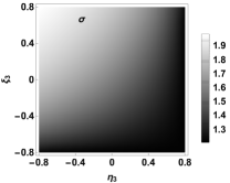
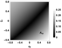
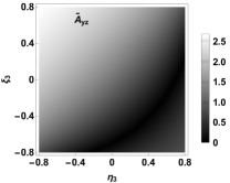
Figure 3: Effect of beam polarizations on sensitivity of cross section $\sigma$, $A_{xy}$ and $\widetilde{A}_{yz}$ in the process $e^{+}e^{-}\to ZZ$ for anomalous couplings $\vec{f}=\{+3,+3,+3,+3\}\times 10^{-3}$ at $\sqrt{s}=500$ GeV and ${\cal L}=100$ fb^-1

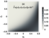
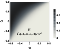
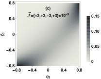
Figure 4: Likelihood $\text{L}({\{\cal O}\},\vec{f};\eta_{3},\xi_{3})$ for three different benchmark anomalous couplings at $\sqrt{s}=500$ GeV and ${\cal L}=100$ fb^-1 in $ZZ$ process

We study the sensitivity of all the observables and their dependence on the beam polarizations at $\sqrt{s}=500$ GeV. Choosing a benchmark value for the anomalous couplings to be

$$\vec{f}=\{f_{4}^{\gamma},f_{4}^{Z},f_{5}^{\gamma},f_{5}^{Z}\}=\{+3,+3,+3,+3\}\times 10^{-3}\ \ ,$$

we show the sensitivities for $\sigma$, $A_{xy}$ and $\widetilde{A}_{yz}$ in Fig. 3 as a function of beam polarizations. The sensitivities for cross section and $\widetilde{A}_{yz}$ peak at the left-top corner of the plots. For $A_{xy}$ sensitivity peak at the right-bottom corner, it is not much smaller in the left-top corner either. The sensitivities of all other asymmetries (not shown here) except $\widetilde{A}_{z}$ peaks at the left-top corner although the exact dependence on the beam polarization may differ. Thus, the combined sensitivity of all the observables is high on the left-top corner of the polarization plane making $(\eta_{3},\xi_{3})=(-0.8,+0.8)$ the best-choice for the chosen benchmark coupling. This best-choice, however, strongly depends upon the values of the anomalous couplings. We note that the best-choice of the beam polarization is mainly decided by the behaviour of the cross section because most of the asymmetries also have similar dependences on the beam polarizations. This, however, does not mean that the cross section provides a best sensitivity or the limits. For example, in Fig. 3 we can see that $\widetilde{A}_{yz}$ has a better sensitivity than the cross section. For the $Z\gamma$ process with the benchmark point

$$\vec{h}=\{h_{1}^{\gamma},h_{1}^{Z},h_{3}^{\gamma},h_{3}^{Z}\}=\{+3,+3,+3,+3\}\times 10^{-3}$$

one obtains similar conclusions: the sensitivities of all observables peak at left-top corner of $\eta_{3}-\xi_{3}$ plane (not shown) except for $\widetilde{A}_{z}$.

For a complete analysis we need to use all the observables simultaneously. To this end we define a likelihood function considering the set of all the observables depending on the anomalous coupling $\vec{f}$ as

$$\text{L}({\{\cal O}\},\vec{f};\eta_{3},\xi_{3})=\exp{\bigg{[}-\frac{1}{2}\sum_{i}{\cal S}({\cal O}_{i}(\vec{f},\eta_{3},\xi_{3}))^{2}\bigg{]}}\ \ ,$$ (17)

$i$ runs over the set of observables in a process. Maximum sensitivity of observables requires the likelihood to be minimum. The likelihood defined here is proportional to the $p$-value and hence the best-choice of beam polarizations comes from the minimum likelihood or maximum distinguishability.

The beam polarization dependence of the likelihood for the $ZZ$ process at the above chosen anomalous couplings is given in Fig. 4(a). The minimum of the likelihood falls in the left-top corner of the $\eta_{3}-\xi_{3}$ plane as expected as most of the observables has higher sensitivity at this corner. For different anomalous couplings the minimum likelihood changes its position in the $\eta_{3}-\xi_{3}$ plane. We have checked the likelihood for $16$ different corners of

$$\vec{f}_{\pm\pm\pm\pm}=\{\pm 3,\pm 3,\pm 3,\pm 3\}\times 10^{-3}$$

and they have different dependences on $\eta_{3},\xi_{3}$. Here we present the likelihood for three different choices of the anomalous couplings in Fig. 4. In Fig. 4(b), the minimum of the likelihood falls in the right-bottom corner where most of the observables have higher sensitivity. In Fig. 4(c) low likelihood falls in both diagonal corners in the $\eta_{3}-\xi_{3}$ plane. This is because some of the observables prefer the left-top corner, while others prefer the right-bottom corner of the polarization plane for higher sensitivity. We have a similar behaviour for the likelihood in the $Z\gamma$ process.

As the anomalous couplings change, the minimum likelihood region changes accordingly and hence the best-choice of beam polarizations. So the best-choice for the beam polarizations depends on the new physics in the process. If one knows the new physics one could tune the beam polarizations to have the best sensitivity for the analysis. But in order to have a suitable choice of beam polarizations irrespective of the possible new physics one needs to minimize the likelihood averaged over all the anomalous couplings. The likelihood function averaged over a volume in parameter space $V_{\vec{f}}$ would be defined as

$$L(V_{\vec{f}},{\{\cal O}\};\eta_{3},\xi_{3})=\int_{V_{\vec{f}}}\text{L}({\{\cal O}\},\vec{f};\eta_{3},\xi_{3})d\vec{f}.$$ (18)

This quantity is nothing but the weighted volume of the parameter space that is statistically consistent with the SM. The size of this weighted volume determines the limits on the parameters. The beam polarizations with the minimum averaged likelihood (or minimum weighted volume) is expected to be the average best choice for any new physics in the process. For numerical analysis we choose the volume to be a hypercube in the $4$ dimensional parameter space with sides equal to $2\times 0.05$ (much larger than the available limits on them) in both the processes. The contribution to the average likelihood from the region outside this volume is negligible.

Table 1: List of simultaneous limits on anomalous couplings obtained for $\sqrt{s}=500$ GeV and $L=100$ fb^-1 for different $\eta_{3}$ and $\xi_{3}$ from MCMC in $ZZ$ process

Beam polarizations	Limits on couplings ($10^{-3}$)
	$f_{4}^{\gamma}$		$f_{4}^{Z}$		$f_{5}^{\gamma}$		$f_{5}^{Z}$
$(\eta_{3},\xi_{3})$	$68~{}\%$	$95~{}\%$	$68~{}\%$	$95~{}\%$	$68~{}\%$	$95~{}\%$	$68~{}\%$	$95~{}\%$	Comments
$-0.80,+0.80$	${}_{-9.3}^{+7.3}$	${}_{-12.0}^{+13.0}$	${}_{-14.0}^{+15.0}$	${}_{-19.0}^{+18.0}$	$\pm 7.3$	$\pm 13.0$	$\pm 11.0$	${}_{-18.0}^{+19.0}$
$-0.40,+0.40$	$\pm 3.1$	${}_{-5.7}^{+5.8}$	$\pm 4.4$	${}_{-8.4}^{+8.2}$	$\pm 3.3$	${}_{-6.2}^{+6.3}$	${}_{-5.2}^{+4.5}$	${}_{-8.5}^{+9.3}$
$0.00,~{}~{}~{}0.00$	$\pm 1.7$	$\pm 3.3$	$\pm 2.5$	$\pm 4.8$	$\pm 1.9$	${}_{-3.6}^{+3.7}$	${}_{-2.7}^{+2.3}$	${}_{-4.6}^{+5.1}$	Unpolarized point
$+0.09,-0.10$	$\pm 1.7$	$\pm 3.2$	$\pm 2.4$	${}_{-4.6}^{+4.7}$	$\pm 1.8$	${}_{-3.4}^{+3.5}$	${}_{-2.6}^{+2.2}$	${}_{-4.5}^{+4.9}$	$P_{Z\gamma}$, best-choice for $Z\gamma$
$+0.12,-0.12$	$\pm 1.6$	$\pm 3.1$	$\pm 2.4$	$\pm 4.7$	$\pm 1.8$	${}_{-3.4}^{+3.5}$	${}_{-2.6}^{+2.2}$	${}_{-4.5}^{+5.0}$	$P_{best}$, combined best-choice
$+0.16,-0.16$	$\pm 1.6$	$\pm 3.1$	$\pm 2.4$	$\pm 4.7$	$\pm 1.8$	${}_{-3.4}^{+3.5}$	${}_{-2.7}^{+2.3}$	${}_{-4.5}^{+5.1}$	$P_{ZZ}$, best-choice for $ZZ$
$+0.40,-0.40$	$\pm 1.9$	$\pm 3.7$	$\pm 3.2$	${}_{-6.2}^{+6.1}$	$\pm 2.1$	${}_{-4.1}^{+4.0}$	${}_{-3.7}^{+3.1}$	${}_{-6.0}^{+6.7}$
$+0.80,-0.80$	${}_{-6.2}^{+5.3}$	${}_{-9.3}^{+9.8}$	${}_{-12.0}^{+9.7}$	${}_{-17.0}^{+18.0}$	$\pm 5.4$	${}_{-9.9}^{+9.5}$	$\pm 9.9$	${}_{-18.0}^{+17.0}$

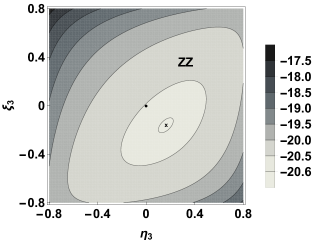
Figure 5: The log of average likelihood, $\log[L(V_{\vec{f}},{\{\cal O}\};\eta_{3},\xi_{3})]$ as a function of beam polarization is shown for the $ZZ$ process at $\sqrt{s}=500$ GeV and ${\cal L}=100$ fb^-1. The dot at the centre is the ($0,0$) point, while cross mark at $P_{ZZ}=(+0.16,-0.16)$ is the minimum likelihood point and hence the best-choice of beam polarizations for $ZZ$ process

The average likelihood $L(V_{\vec{f}},{\{\cal O}\};\eta_{3},\xi_{3})$ in the $ZZ$ process as a function of beam polarization is shown in Fig. 5 on $\log$-scale. The dot on the middle of the plot represents the unpolarized case and the cross mark at $P_{ZZ}=(+0.16,-0.16)$ represents the minimum averaged likelihood point i.e., the best-choice of beam polarizations. The unpolarized point, the best point and the points within two central contour in Fig. 5 have the same order of average likelihood and expected to give similar limits on anomalous couplings. The polarization point from darker contours corresponds to larger values of average likelihood and expected to give relatively looser limits on anomalous couplings. To explore this we estimate simultaneous limits using Markov-Chain-Monte-Carlo (MCMC) method at $P_{ZZ}$, unpolarized beam and few other benchmark choice of beam polarizations. The limits thus obtained on the anomalous couplings for the $ZZ$ process are listed in Table 1. We note that the limits for the best-choice of polarizations ($P_{ZZ}$) are best but comparable to other nearby benchmark beam polarization including the unpolarized beams. This is due to the fact that the average likelihood is comparable for these cases. Further, the limits for $(+0.4,-0.4)$ and $(-0.4,+0.4)$ are increasingly bad as these points correspond to the third and fourth contours, i.e., we have increasingly larger average likelihood. The point $(-0.8,+0.8)$ has the largest average likelihood and the corresponding limits are the worst in Table 1. We also note that the limits for the unpolarized case in Table 1 are better than the ones reported in Ref. Rahaman:2016pqj , when adjusted for the systematic errors. This improvement here is due to the inclusion of three new non-vanishing asymmetries $\widetilde{A}_{z}$, $\widetilde{A}_{xz}$ and $\widetilde{A}_{yz}$. Of these, $\widetilde{A}_{xz}$ has linear dependence on $f_{5}^{\gamma,Z}$ with larger sensitivity to $f_{5}^{Z}$ leading to about $30~{}\%$ improvement in the limit. Similarly, the $CP$-odd asymmetry $\widetilde{A}_{yz}$ has a linear dependence on $f_{4}^{\gamma,Z}$ with larger sensitivity to $f_{4}^{Z}$ and this again leads to about $30~{}\%$ improvement in the corresponding limit. The asymmetry $\widetilde{A}_{z}$ has a quadratic dependence on all four parameters and has too poor sensitivity for all of them to be useful.

We do a similar analysis for the $Z\gamma$ process. The average likelihood $L(V_{\vec{h}},{\{\cal O}\};\eta_{3},\xi_{3})$ is shown in Fig. 6 on log-scale. Here also the dot on the middle of the plot is for unpolarized case while the plus mark at $P_{Z\gamma}=(+0.09,-0.10)$ is for the minimum averaged likelihood and hence the best-choice of beam polarizations. The corresponding simultaneous limits on the anomalous couplings $h_{i}$ are presented in Table 2.Again we notice that the limits obtained for the best-choice of the beam polarizations $P_{Z\gamma}$ are tighter than any other point on the polarization plane, yet comparable to the nearby polarization points within the two central contours in Fig. 6, including the unpolarized point. This again is due to the comparable values of the averaged likelihood of the two central contours containing $P_{Z\gamma}$ and the unpolarized point. The limits at the points $(+0.4,-0.4)$ and $(-0.4,+0.4)$ are worse as they fall in the fourth and fifth contour containing much larger likelihood values. Like the $ZZ$ case the point $(-0.8,+0.8)$ has the largest average likelihood and the corresponding limits are the worst. The simultaneous limits for the unpolarized case (also the $P_{Z\gamma}$) turns out to be much better than the ones reported in Ref. Rahaman:2016pqj for $h_{1,3}^{\gamma}$ due to the inclusions of new asymmetries in the present analysis. The $CP$-odd asymmetry $\widetilde{A}_{yz}$ has linear dependence on $h_{1}^{\gamma,Z}$ with a large sensitivity towards $h_{1}^{\gamma}$ leading to an improvement in the corresponding limit by a factor of two compare to earlier report when adjusted for systematic errors. The limit on $h_{3}^{\gamma}$ improves by a factor of $3$ owing to the asymmetry $\widetilde{A}_{xz}$. The limits on $h_{1,3}^{Z}$ remain comparable.

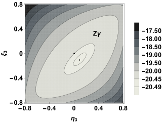
Figure 6: Same as Fig. 5 but for the $Z\gamma$ process. The plus mark at $P_{Z\gamma}=(+0.09,-0.10)$ is the lowest likelihood point and hence the best-choice of beam polarizations for $Z\gamma$ process

Table 2: List of simultaneous limits on anomalous couplings obtained for $\sqrt{s}=500$ GeV and $L=100$ fb^-1 for different $\eta_{3}$ and $\xi_{3}$ from MCMC in $Z\gamma$ process

Beam polarizations	Limits on couplings ($10^{-3}$)
	$h_{1}^{\gamma}$		$h_{1}^{Z}$		$h_{3}^{\gamma}$		$h_{3}^{Z}$
$(\eta_{3},\xi_{3})$	$68~{}\%$	$95~{}\%$	$68~{}\%$	$95~{}\%$	$68~{}\%$	$95~{}\%$	$68~{}\%$	$95~{}\%$	Comments
$-0.80,+0.80$	${}_{-9.3}^{+7.7}$	$\pm 13.0$	$\pm 11.0$	${}_{-19.0}^{+18.0}$	$\pm 7.5$	$\pm 13.0$	$\pm 11.0$	$\pm 19.0$
$-0.40,+0.40$	$\pm 3.9$	${}_{-7.5}^{+7.4}$	$\pm 6.5$	$\pm 12.0$	${}_{-3.7}^{+4.4}$	${}_{-8.0}^{+7.1}$	$\pm 6.6$	${}_{-12.0}^{+13.0}$
$0.00,~{}~{}~{}0.00$	$\pm 1.6$	$\pm 3.1$	$\pm 3.7$	${}_{-7.0}^{+7.1}$	${}_{-1.4}^{+1.6}$	${}_{-3.0}^{+2.8}$	$\pm 3.6$	$\pm 7.1$	Unpolarized point
$+0.09,-0.10$	$\pm 1.5$	$\pm 2.9$	$\pm 3.6$	$\pm 7.0$	${}_{-1.3}^{+1.4}$	${}_{-2.8}^{+2.6}$	$\pm 3.6$	${}_{-7.1}^{+7.0}$	$P_{Z\gamma}$, best-choice for $Z\gamma$
$+0.12,-0.12$	$\pm 1.5$	$\pm 2.9$	$\pm 3.7$	$\pm 7.1$	$\pm 1.4$	${}_{-2.8}^{+2.6}$	$\pm 3.6$	$\pm 7.1$	$P_{best}$, combined best-choice
$+0.16,-0.16$	$\pm 1.5$	$\pm 3.0$	$\pm 3.7$	${}_{-7.3}^{+7.2}$	${}_{-1.3}^{+1.5}$	${}_{-2.8}^{+2.6}$	$\pm 3.7$	${}_{-7.3}^{+7.1}$	$P_{ZZ}$, best-choice for $ZZ$
$+0.40,-0.40$	$\pm 2.4$	$\pm 4.6$	$\pm 5.2$	$\pm 10.0$	${}_{-2.2}^{+2.5}$	${}_{-4.7}^{+4.3}$	$\pm 5.2$	$\pm 10.0$
$+0.80,-0.80$	$\pm 5.8$	${}_{-9.9}^{+10.0}$	${}_{-13.0}^{+11.0}$	${}_{-18.0}^{+19.0}$	${}_{-7.2}^{+5.8}$	${}_{-9.7}^{+10.0}$	${}_{-15.0}^{+13.0}$	${}_{-18.0}^{+19.0}$

The combined analysis of the processes $ZZ$ and $Z\gamma$ is expected to change the best-choice of beam polarizations and limits accordingly. For the average likelihood for these two processes the volume, in which one should average, will change to $V_{\vec{f}/\vec{h}}\to V_{\vec{F}}$, where $\vec{F}=\{\vec{f},\vec{h}\}$ and observables from both processes should be added to the likelihood defined in Eq. 17. The combined averaged likelihood showing dependence on the beam polarizations for the two processes considered here is shown in Fig. 7. The dot on the middle of the plot is for the unpolarized case and asterisk mark at $P_{best}=(+0.12,-0.12)$ is the combined best-choice of beam polarizations. Other points are due to $P_{ZZ}$ and $P_{Z\gamma}$. The combined best-choice point sits in between $P_{ZZ}$ and $P_{Z\gamma}$. The limits, presented in Table 1 and 2, at the combined best-choice of the beam polarizations are slightly weaker than the limit at the best-choice points but comparable in both processes as expected. Thus the combined best-choice can be a good benchmark beam polarizations for the process $ZZ$ and $Z\gamma$ to study at ILC.

The best-choice of beam polarizations, obtained here, depends on the size of the estimated error of the observables and hence on the systematics $\epsilon_{\sigma}$ and $\epsilon_{A}$. Numerical analysis shows that the best-choice points, for both processes separately and combined, move away from the unpolarized point along the cross diagonal axis towards the right-bottom corner on the $\eta_{3}-\xi_{3}$ plane when $\epsilon_{\sigma}$ or $\epsilon_{A}$ or both are increased. For example, if we double $\epsilon_{\sigma}$ and $\epsilon_{A}$ both, i.e. we take $\epsilon_{\sigma}=0.04$ and $\epsilon_{A}=0.02$, the best-choice points $P_{ZZ}$, $P_{Z\gamma}$ and $P_{best}$ become ($+0.20,-0.20$), ($+0.13,-0.12)$ and ($+0.17,-0.16$), respectively. On the other hand the best-choice points move towards the unpolarized point as the systematics are decreased. For example, when the systematics are reduced by $1/2$, i.e. for $\epsilon_{\sigma}=0.01$ and $\epsilon_{A}=0.005$, the best-choice points for $ZZ$, $Z\gamma$ and for combined process move to ($+0.15,-0.15$), ($+0.08,-0.08$) and ($+0.11,-0.11$), respectively. However, the best-choice points do not move further closer to the unpolarized point when the size of systematics becomes smaller than the statistical one.

Similar analysis as presented in Fig. 7 can be done by combining many processes, as one should do, to choose a suitable beam polarizations at ILC. For many processes (e.g., we can include $WW$ production with anomalous couplings among charged gauge boson) with different couplings, the volume in which one should do the average will change to $V_{\vec{f}/\vec{h}}=V_{\vec{F}}$, where $\vec{F}$ would be the set of all couplings for all the processes considered. The set of observables $\{\mathcal{O}\}$ would include all the relevant observables from all the processes combined in the expression for the likelihood.

Figure 7: The log of average likelihood, $\log[L(V_{\{\vec{f},\vec{h}\}},{\{\cal O}\};\eta_{3},\xi_{3})]$, is shown considering both the processes $ZZ$ and $Z\gamma$ at $\sqrt{s}=500$ GeV, ${\cal L}=100$ fb^-1. The asterisk mark at $P_{best}=(+0.12,-0.12)$ is the combined best-choice for beam polarizations while the other points are for $ZZ$ (cross mark) and $Z\gamma$ (plus mark)

4 Conclusion

To summarize, we aim to find the best-choice of beam polarization for an $e^{+}e^{-}$ collider to probe the anomalous couplings in the neutral gauge-boson sector in the $ZZ$ and $Z\gamma$ processes. We study the effects of beam polarization on polarization asymmetries and corresponding sensitivities towards anomalous couplings. Using the minimum averaged likelihood, we find the best-choice of the beam polarization for the two processes and also the combined best-choice. Here the list of observables includes the cross section along with eight polarization asymmetries for the $Z$ boson. Simultaneous limits on anomalous couplings were obtained using the MCMC method for a set of benchmark beam polarization including the best-choices and they are listed in Tables 1 and 2. The limits obtained for the unpolarized case are better than the ones reported in Ref. Rahaman:2016pqj . This is because the present analysis includes three new observables $\widetilde{A}_{z}$, $\widetilde{A}_{xz}$ and $\widetilde{A}_{yz}$. These new asymmetries yield better limits on $f^{Z}_{4,5}$ and $h^{\gamma}_{1,3}$, while we have comparable (yet better) limits on $f^{\gamma}_{4,5}$ and $h^{Z}_{1,3}$. Comparing the limits for various benchmark beam polarizations from Tables 1 and 2, we find that all three best beam polarization choices yield comparable limits and they are comparable to the unpolarized case as well. Thus, as far as anomalous couplings in the neutral gauge-boson sector are concerned, unpolarized beams perform as good as the best choices. This conclusion, however, can change if one includes more or a different set of observables in the analysis or add more processes to the analysis. For example, processes involving $W^{\pm}$ or a Higgs boson may have a different preference for the beam polarization.

Considering the physics impact and the cost of beam polarizations at ILC one may chose the unpolarized beams for the first run, at least for the two processes studied here. But as we infer, a detailed global analysis is required involving other processes as well to conclude this. We further note that the case of transverse beam polarization is not addressed here and conclusions may differ in that case.

Acknowledgements: R. R. thanks Department of Science and Technology, Government of India for support through DST-INSPIRE Fellowship for doctoral program, INSPIRE CODE IF140075, 2014.

References

- (1) CMS Collaboration, S. Chatrchyan et al., Observation of a new boson at a mass of 125 GeV with the CMS experiment at the LHC, Phys. Lett. B716 (2012) 30–61, arXiv:1207.7235 [hep-ex].
- (2) ILC Collaboration, G. Aarons et al., International Linear Collider Reference Design Report Volume 2: Physics at the ILC, arXiv:0709.1893 [hep-ph].
- (3) H. Baer, T. Barklow, K. Fujii, Y. Gao, A. Hoang, S. Kanemura, J. List, H. E. Logan, A. Nomerotski, M. Perelstein, et al., The International Linear Collider Technical Design Report - Volume 2: Physics, arXiv:1306.6352 [hep-ph].
- (4) T. Behnke, J. E. Brau, B. Foster, J. Fuster, M. Harrison, J. M. Paterson, M. Peskin, M. Stanitzki, N. Walker, and H. Yamamoto, The International Linear Collider Technical Design Report - Volume 1: Executive Summary, arXiv:1306.6327 [physics.acc-ph].
- (5) G. Moortgat-Pick et al., The Role of polarized positrons and electrons in revealing fundamental interactions at the linear collider, Phys. Rept. 460 (2008) 131–243, arXiv:hep-ph/0507011 [hep-ph].
- (6) V. V. Andreev, G. Moortgat-Pick, P. Osland, A. A. Pankov, and N. Paver, Discriminating Z’ from Anomalous Trilinear Gauge Coupling Signatures in at ILC with Polarized Beams, Eur. Phys. J. C72 (2012) 2147, arXiv:1205.0866 [hep-ph].
- (7) B. Ananthanarayan, M. Patra, and P. Poulose, Signals of additional Z boson in at the ILC with polarized beams, JHEP 02 (2011) 043, arXiv:1012.3566 [hep-ph].
- (8) P. Osland, A. A. Pankov, and A. V. Tsytrinov, Identification of extra neutral gauge bosons at the International Linear Collider, Eur. Phys. J. C67 (2010) 191–204, arXiv:0912.2806 [hep-ph].
- (9) A. A. Pankov, N. Paver, and A. V. Tsytrinov, Distinguishing new physics scenarios at a linear collider with polarized beams, Phys. Rev. D73 (2006) 115005, arXiv:hep-ph/0512131 [hep-ph].
- (10) O. Kittel, G. Moortgat-Pick, K. Rolbiecki, P. Schade, and M. Terwort, Measurement of CP asymmetries in neutralino production at the ILC, Eur. Phys. J. C72 (2012) 1854, arXiv:1108.3220 [hep-ph].
- (11) H. K. Dreiner, O. Kittel, and A. Marold, Normal tau polarisation as a sensitive probe of CP violation in chargino decay, Phys. Rev. D82 (2010) 116005, arXiv:1001.4714 [hep-ph].
- (12) A. Bartl, K. Hohenwarter-Sodek, T. Kernreiter, and O. Kittel, CP asymmetries with longitudinal and transverse beam polarizations in neutralino production and decay into the Z0 boson at the ILC, JHEP 09 (2007) 079, arXiv:0706.3822 [hep-ph].
- (13) K. Rao and S. D. Rindani, Probing CP-violating contact interactions in e+ e- —¿ HZ with polarized beams, Phys. Lett. B642 (2006) 85–92, arXiv:hep-ph/0605298 [hep-ph].
- (14) A. Bartl, H. Fraas, S. Hesselbach, K. Hohenwarter-Sodek, T. Kernreiter, and G. A. Moortgat-Pick, CP-odd observables in neutralino production with transverse e+ and e- beam polarization, JHEP 01 (2006) 170, arXiv:hep-ph/0510029 [hep-ph].
- (15) H. Czyz, K. Kolodziej, and M. Zralek, Composite Boson and CP Violation in the Process , Z. Phys. C43 (1989) 97.
- (16) D. Choudhury and S. D. Rindani, Test of CP violating neutral gauge boson vertices in , Phys. Lett. B335 (1994) 198–204, arXiv:hep-ph/9405242 [hep-ph].
- (17) B. Ananthanarayan, S. D. Rindani, R. K. Singh, and A. Bartl, Transverse beam polarization and CP-violating triple-gauge-boson couplings in , Phys. Lett. B593 (2004) 95–104, arXiv:hep-ph/0404106 [hep-ph]. [Erratum: Phys. Lett.B608,274(2005)].
- (18) B. Ananthanarayan, S. K. Garg, M. Patra, and S. D. Rindani, Isolating CP-violating ZZ coupling in Z with transverse beam polarizations, Phys. Rev. D85 (2012) 034006, arXiv:1104.3645 [hep-ph].
- (19) B. Ananthanarayan and S. D. Rindani, CP violation at a linear collider with transverse polarization, Phys. Rev. D70 (2004) 036005, arXiv:hep-ph/0309260 [hep-ph].
- (20) S. Groote, J. G. Korner, B. Melic, and S. Prelovsek, A survey of top quark polarization at a polarized linear collider, Phys. Rev. D83 (2011) 054018, arXiv:1012.4600 [hep-ph].
- (21) M. S. Amjad et al., A precise characterisation of the top quark electro-weak vertices at the ILC, Eur. Phys. J. C75 no. 10, (2015) 512, arXiv:1505.06020 [hep-ex].
- (22) B. Ananthanarayan, M. Patra, and P. Poulose, W physics at the ILC with polarized beams as a probe of the Littlest Higgs Model, JHEP 11 (2009) 058, arXiv:0909.5323 [hep-ph].
- (23) B. Ananthanarayan, M. Patra, and P. Poulose, Probing strongly interacting W’s at the ILC with polarized beams, JHEP 03 (2012) 060, arXiv:1112.5020 [hep-ph].
- (24) S. Kumar, P. Poulose, and S. Sahoo, Study of Higgs-gauge boson anomalous couplings through at ILC, Phys. Rev. D91 no. 7, (2015) 073016, arXiv:1501.03283 [hep-ph].
- (25) S. D. Rindani and P. Sharma, Decay-lepton correlations as probes of anomalous ZZH and gammaZH interactions in e+e- –¿ ZH with polarized beams, Phys. Lett. B693 (2010) 134–139, arXiv:1001.4931 [hep-ph].
- (26) S. S. Biswal and R. M. Godbole, Use of transverse beam polarization to probe anomalous VVH interactions at a Linear Collider, Phys. Lett. B680 (2009) 81–87, arXiv:0906.5471 [hep-ph].
- (27) S. D. Rindani and P. Sharma, Angular distributions as a probe of anomalous ZZH and gammaZH interactions at a linear collider with polarized beams, Phys. Rev. D79 (2009) 075007, arXiv:0901.2821 [hep-ph].
- (28) R. Rahaman and R. K. Singh, On polarization parameters of spin-1 particles and anomalous couplings in , Eur. Phys. J. C76 no. 10, (2016) 539, arXiv:1604.06677 [hep-ph].
- (29) F. Boudjema and R. K. Singh, A Model independent spin analysis of fundamental particles using azimuthal asymmetries, JHEP 07 (2009) 028, arXiv:0903.4705 [hep-ph].
- (30) J. A. Aguilar-Saavedra and J. Bernabeu, Breaking down the entire W boson spin observables from its decay, Phys. Rev. D93 no. 1, (2016) 011301, arXiv:1508.04592 [hep-ph].
- (31) F. Boudjema, Proc. of the Workshop on Collisions at 500GeV: The Physics Potential, edited by P.M. Zerwas, DESY (1992) 757.
- (32) U. Baur and E. L. Berger, Probing the weak boson sector in production at hadron colliders, Phys. Rev. D47 (1993) 4889–4904.
- (33) J. Ellison and J. Wudka, Study of trilinear gauge boson couplings at the Tevatron collider, Ann. Rev. Nucl. Part. Sci. 48 (1998) 33–80, arXiv:hep-ph/9804322 [hep-ph].
- (34) U. Baur and D. L. Rainwater, Probing neutral gauge boson selfinteractions in production at hadron colliders, Phys. Rev. D62 (2000) 113011, arXiv:hep-ph/0008063 [hep-ph].
- (35) B. Ananthanarayan and S. D. Rindani, New physics in with polarized beams, JHEP 10 (2005) 077, arXiv:hep-ph/0507037 [hep-ph].
- (36) H. Aihara et al., Anomalous gauge boson interactions, arXiv:hep-ph/9503425 [hep-ph].
- (37) G. J. Gounaris, J. Layssac, and F. M. Renard, Off-shell structure of the anomalous and selfcouplings, Phys. Rev. D65 (2002) 017302, arXiv:hep-ph/0005269 [hep-ph]. [Phys. Rev.D62,073012(2000)].
- (38) P. Poulose and S. D. Rindani, CP violating and top quark electric dipole couplings in , Phys. Lett. B452 (1999) 347–354, arXiv:hep-ph/9809203 [hep-ph].
- (39) A. Senol, and anomalous couplings in collision at the LHC, Phys. Rev. D87 (2013) 073003, arXiv:1301.6914 [hep-ph].
- (40) I. Ots, H. Uibo, H. Liivat, R. Saar, and R. K. Loide, Possible anomalous Z Z gamma and Z gamma gamma couplings and Z boson spin orientation in : The role of transverse polarization, Nucl. Phys. B740 (2006) 212–221.
- (41) B. Ananthanarayan, J. Lahiri, M. Patra, and S. D. Rindani, New physics in at the ILC with polarized beams: explorations beyond conventional anomalous triple gauge boson couplings, JHEP 08 (2014) 124, arXiv:1404.4845 [hep-ph].
- (42) G. J. Gounaris, J. Layssac, and F. M. Renard, Signatures of the anomalous and production at the lepton and hadron colliders, Phys. Rev. D61 (2000) 073013, arXiv:hep-ph/9910395 [hep-ph].
- (43) S. Y. Choi, Probing the weak boson sector in , Z. Phys. C68 (1995) 163–172, arXiv:hep-ph/9412300 [hep-ph].
- (44) T. G. Rizzo, Polarization asymmetries in gamma e collisions and triple gauge boson couplings revisited, in Physics and experiments with future linear e+ e- colliders. Proceedings, 4th Workshop, LCWS’99, Sitges, Spain, April 28-May 5, 1999. Vol. 1: Physics at linear colliders, pp. 529–533. 1999. arXiv:hep-ph/9907395 [hep-ph]. http://www-public.slac.stanford.edu/sciDoc/docMeta.aspx?slacPubNumber=SLAC-PUB-8192.
- (45) S. Atag and I. Sahin, ZZ gamma and Z gamma gamma couplings in gamma e collision with polarized beams, Phys. Rev. D68 (2003) 093014, arXiv:hep-ph/0310047 [hep-ph].
- (46) CMS Collaboration, V. Khachatryan et al., Measurements of the production cross sections in the channel in proton–proton collisions at and and combined constraints on triple gauge couplings, Eur. Phys. J. C75 no. 10, (2015) 511, arXiv:1503.05467 [hep-ex].
- (47) ATLAS Collaboration, G. Aad et al., Measurements of and production in collisions at 8 TeV with the ATLAS detector, Phys. Rev. D93 no. 11, (2016) 112002, arXiv:1604.05232 [hep-ex].