The Lamb shift and the gravitational binding energy
for binary black holes

Rafael A. Porto
ICTP South American Institute for Fundamental Research
Rua Dr. Bento Teobaldo Ferraz 271, 01140-070 São Paulo, SP Brazil

  We show that the correction to the gravitational binding energy for binary black holes due to the tail effect resembles the Lamb shift in the Hydrogen atom. In both cases a conservative effect arises from interactions with radiation modes, and moreover an explicit cancelation between near and far zone divergences is at work. In addition, regularization scheme-dependence may introduce ‘ambiguity parameters’. This is remediated –within an effective field theory approach– by the implementation of the zero-bin subtraction. We illustrate the procedure explicitly for the Lamb shift, by performing an ambiguity-free derivation within the framework of non-relativistic electrodynamics. We also derive the renormalization group equations from which we reproduce Bethe logarithm (at order $\alpha_{e}^{5}\log\alpha_{e}$), and likewise the contribution to the gravitational potential from the tail effect (proportional to $v^{8}\log v$).  

1 Introduction

Binary coalescences are posed to become standard sources for present and future gravitational wave (GW) observatories [1, 2, 3]. GW astronomy will map the contents of the universe to an unprecedented level [4, 5], addressing fundamental problems in astrophysics and cosmology. The searches demand state-of-the-art numerical and analytical modeling, to enable the most precise parameter estimation [6, 7, 8]. Motivated by the construction of an accurate template bank, the effective field theory (EFT) framework was introduced to solve for the gravitational dynamics of inspiralling binary systems to high level of precision [9, 10, 11, 12, 13, 14, 15, 16]. The EFT approach was originally coined Non-Relativistic General Relativity (NRGR) [9], following similarities with the techniques used for the strong interaction (NRQCD), as well as electrodynamics (NRQED). NRGR has enabled the computation of all the ingredients for the GW phase for spinning compact binary systems up to third Post-Newtonian (3PN) order [17, 18, 19, 20, 21, 22, 23, 24, 25, 16]. In addition, significant progress has been achieved towards 4PN accuracy in the EFT approach, both for non-spinning [26, 27, 28] and rotating bodies [29, 30]. Some of these results have been obtained using other (more traditional) methods, see e.g. [6, 7] for references.

The gravitational binding potential for binary systems has been recently computed in the Arnowitt, Deser, and Misner (ADM) and ‘Fokker-action’ approaches up to 4PN order for non-spinning bodies [31, 32, 33, 34, 35, 36, 37]. Despite the remarkable feat, the derivation could not be completed at first, because of regularization ambiguities. Hence, the final expression was obtained after comparison with gravitational self-force calculations [33, 36], see also [38]. In a companion paper [39] we describe the procedure which yields the gravitational potential, in NRGR, without the need of ‘ambiguity parameters’. The purpose of the present paper is to demonstrate that the issue at hand is actually more common than it might seem, since similar considerations apply in electrodynamics, and in particular in the derivation of the Lamb shift [40, 41, 42, 43, 44]. As we shall see, by performing the calculation within the EFT approach NRQED, both infrared (IR) and ultraviolet (UV) divergences are present, as in the gravitational case. We perform the zero-bin subtraction [45] and arrive at an ambiguity-free result. We also derive the renormalization group equation for the binding potential, and readily obtain Bethe logarithm. We then show how the manipulations in electrodynamics closely resemble the computations in gravity. In particular, the renormalization group evolution and logarithmic contributions to the binding energy may be obtained in both cases without worrying about the subtleties of the matching conditions [28]. Throughout this paper we work in $c=\hbar=1$ units, unless otherwise noted.

2 The (quantum) binding energy in electrodynamics

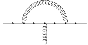
Figure 1: One loop vertex correction in electrodynamics.

Quantum effects in QED contribute to the binding energy of the Hydrogen atom. A celebrated example is the Lamb shift [40, 41, 42, 43, 44], which involves a one-loop vertex correction, see fig. 1. Here we perform the computation using an EFT approach, highlighting the similarities with the binary inspiral case. We show the existence of IR/UV divergences, discuss the zero-bin subtraction and lack of ambiguities, and the renormalization group structure.

2.1 Form factors

The full QED vertex (including wave-function renormalization) can be expressed in terms of two form factors,

$$-ie\bar{u}(p_{1})\,\left[F_{1}(q^{2})\gamma^{\mu}+\frac{i}{2m_{e}}F_{2}(q^{2})\sigma^{\mu\nu}q_{\nu}\right]u(p_{2})\,,$$ (2.1)

with $q=p_{1}-p_{2}$, $\gamma^{\mu}$ the Dirac matrices, $\sigma^{\mu\nu}\equiv\frac{i}{2}[\gamma^{\mu},\gamma^{\nu}]$, and $u(p)$ a Dirac spinor. The expressions for $F_{1},F_{2}$ are divergent, and in dimensional regularization (dim. reg.) are given by, e.g. [46],

$$F_{1}(q^{2}) = 1-\frac{\alpha_{e}(\mu)}{\pi}\frac{q^{2}}{m_{e}^{2}}\left[\frac{1}{3\epsilon_{\rm IR}}+\frac{1}{8}-\frac{1}{6}\log\frac{m^{2}_{e}}{\bar{\mu}^{2}}\right]+{\cal O}(q^{4})\,,$$ (2.2)

$$F_{2}(q^{2}) = \frac{\alpha_{e}(\mu)}{2\pi}\left[1+\frac{q^{2}}{6m_{e}^{2}}\right]+{\cal O}(q^{4})\,,$$ (2.3)

where $\alpha_{e}\equiv e^{2}(\mu)/4\pi$ is the fine-structure constant, $m_{e}$ the mass of the electron, and we have expanded to order $q^{2}/m_{e}^{2}$ the resulting integrals. The factor of $\bar{\mu}^{2}\equiv 4\pi e^{-\gamma_{E}}\mu^{2}$, with $\gamma_{E}$ the Euler constant, appear in dim. reg. as the ‘subtraction scale’.We will encounter both IR as well as UV divergences, which in dim. reg. emerge as poles in $\epsilon_{\rm IR/UV}\equiv(d-4)_{\rm IR/UV}$, as we approach $d=4$ dimensions. While intermedia UV divergences are present, the final expressions for the form factors are UV finite, featuring instead an IR pole (often regularized with a photon mass).

From (2.2) and (2.3) we can derive for instance the one-loop correction to the scattering amplitude in QED, and the Lamb shift. However, in order to draw parallels with computations in gravity, in what follows we will perform the calculation within the framework of non-relativistic QED (NRQED).

2.2 The EFT framework: NRQED

In addition to the electron’s mass, we have two other relevant scales in the bound state problem. There is Bohr’s radius,

$$r_{B}\simeq 1/(m_{e}v),$$ (2.4)

with $v$ the relative velocity, and the typical frequency scale given by the Rydberg energy

$$E\simeq m_{e}v^{2},$$ (2.5)

which determines the split between levels. In a bound state the virial theorem implies

$$\alpha_{e}/r_{B}\sim m_{e}v^{2}\to\alpha_{e}\sim v.$$ (2.6)

After one eliminates the heavy scale in the theory, $m_{e}$, as in the heavy quark effective theory (HQET), we are left with three relevant regions [48, 49, 50]: potential modes scaling as

$$(p_{\rm pot}^{0},{\bm{p}}_{\rm pot})\sim(m_{e}v^{2},m_{e}v)\sim(v/r_{B},1/r_{B})\,,$$ (2.7)

soft modes,

$$(p_{S}^{0},{\bm{p}}_{S})\sim(m_{e}v,m_{e}v)\sim(1/r_{B},1/r_{B})\,,$$ (2.8)

and ultra-soft ones,

$$(p_{US}^{0},{\bm{p}}_{US})\sim(m_{e}v^{2},m_{e}v^{2})\sim(v/r_{B},v/r_{B})\,.$$ (2.9)

Notice these power counting rules are similar to the ones in NRGR, for potential and radiation fields. The effective Lagrangian density for NRQED takes the form (ignoring spin interactions for simplicity) [51, 46, 50]

$${\cal L}_{\rm NRQED}=-\frac{1}{4}F^{\mu\nu}F_{\mu\nu}+\psi^{v\dagger}_{e}\left(iD_{0}+\frac{{\bm{D}}^{2}}{2m_{e}}+\frac{{\bm{D}}^{4}}{8m^{3}_{e}}+e\frac{c_{V}}{8m_{e}^{2}}\,\bm{\nabla}\cdot{\bm{E}}+\cdots\right)\psi^{v}_{e}+i\psi^{\dagger}_{p}D_{0}\psi_{p}+\cdots\,,$$ (2.10)

where $D_{\mu}$ is the covariant derivative, $\psi^{v}_{e}$ is given by $\psi^{v}_{e}=e^{im_{e}t}\psi_{e}$, as in HQET, and we have kept only the terms which are relevant for our purposes. We have also added the contribution from the proton, $\psi_{p}$, which we treat as a static source, up to ${\cal O}(m_{e}/m_{p})$ corrections. The matching coefficient, $c_{V}$, is given by [46]

$$c_{V}=F_{1}(0)+2F_{2}(0)+8m_{e}^{2}\frac{d}{dq^{2}}F_{1}(0)\,,$$ (2.11)

with the form factors in (2.2) and (2.3). In dim. reg. the expression for $c_{V}$ reads

$$c_{V}=1+\frac{8}{3}\frac{\alpha_{e}(\mu)}{\pi}\left[-\frac{1}{\epsilon_{\rm IR}}+\log m_{e}/\mu\right]\,.$$ (2.12)

Notice we have kept the IR pole explicitly, and will be carried over until the end of the calculation. We will discuss later on in section 2.4 how to properly handle this divergence prior to computing the Lamb shift. As we shall demonstrate, this IR pole will be linked to a UV singularity arising from the ultra-soft sector. (This will be intimately related to cancelation of factors of $\log\mu$.)

The next step is to integrate out the potential and soft modes. This procedure matches NRQED into an effective theory with ultra-soft degrees of freedom only, called ‘potential’ NRQED or pNRQED for short [52]. The binding energy now becomes a matching coefficient. Therefore, we have a Coulomb-type potential of the form [52],

$$\int dt\int d^{3}{\bm{x}}_{1}d^{3}{\bm{x}}_{2}\;\psi_{p}^{\dagger}(t,{\bm{x}}_{1})\psi_{p}(t,{\bm{x}}_{1})\left(\frac{\alpha_{e}}{|{\bm{x}}_{1}-{\bm{x}}_{2}|}\right)\psi_{e}^{\dagger}(t,{\bm{x}}_{2})\psi_{e}(t,{\bm{x}}_{2})\,.$$ (2.13)

For the term proportional to $c_{V}$ we may use Gauss’ law, obtaining [52]

$$-c_{V}\frac{e^{2}}{8m_{e}^{2}}\int dt\int d^{3}{\bm{x}}_{1}d{\bm{x}}_{2}\;\psi_{p}^{\dagger}(t,{\bm{x}}_{1})\psi_{p}(t,{\bm{x}}_{1})\psi_{e}^{\dagger}(t,{\bm{x}}_{2})\psi_{e}(t,{\bm{x}}_{2})\delta^{3}({\bm{x}}_{1}-{\bm{x}}_{2})\,.$$ (2.14)

Since the typical size of the bound state is given by $r_{B}\ll 1/E$, the ultra-soft photon field is multipole expanded in powers of $E\,r_{B}\sim v\sim\alpha_{e}$. This is reminiscent of the construction of the radiation theory in NRGR, in terms of a series of multipole moments [24]. At the end of the day, the relevant pieces in the pNRQED Lagrangian are[46, 52]

$$L_{\rm pNRQED} = \int d^{3}{\bm{x}}\,\psi^{\dagger}(t,{\bm{x}})\left(i\partial_{0}-eA^{0}_{US}(t,0)+e\,{\bm{x}}^{i}\bm{\nabla}_{i}A^{0}_{US}(t,0)+\frac{\bm{\nabla}^{2}}{2m_{e}}-V({\bm{x}})\right.$$

$$\left.-ie\frac{{\bm{A}}_{US}(t,0)\cdot\bm{\nabla}}{m_{e}}-c_{V}\frac{e^{2}}{8m_{e}}\delta^{3}({\bm{x}})\right)\psi(t,{\bm{x}})-\frac{1}{4}\int d^{3}{\bm{x}}\,F_{US}^{\mu\nu}F_{US\,\mu\nu}\,,{}$$

where $V_{e}=-\alpha_{e}/|{\bm{x}}|\,.$ We dropped the tag on the field, which now represents the wave-function of an electron in the background of a static Coulomb-like source with typical energy/momenta of order $m_{e}v^{2}$. Notice the contribution from $c_{V}$ may be thought of as a local renormalization of the potential,

$$\delta V_{e}({\bm{x}})=c_{V}\frac{e^{2}}{8m_{e}}\delta^{3}({\bm{x}})\,.$$ (2.16)

2.3 The Lamb shift

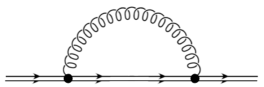
Figure 2: The one-loop correction in (2.22). The double line represents the bound state, and the dots are the dipole-type coupling from (2.2). A similar diagram –albeit at the classical level– appears in NRGR (see below).

The calculation of the Lamb shift can be found in different textbooks, e.g. [54]. Here we derive it following the framework of the EFT approach NRQED. (The use of dim. reg. to regularize the divergences in the computation of the Lamb shift was also advocated in [54, 55, 56].)

The ultra-soft contribution to the $E_{n}$ level of the Hydrogen atom is represented in fig. 2, and is given by a self-energy type diagram. The computation entails the two-point function

$$G(t,{\bm{x}})\equiv-i\langle 0|T(\psi(0)\psi(t,{\bm{x}}))|0\rangle\,,$$ (2.17)

which it is convenient to transform into Fourier space

$$\tilde{G}({\bm{x}},E)=\int dt\,e^{iEt}\,G(t,{\bm{x}})\,.$$ (2.18)

At leading order, introducing a complete set of states, we have

$$\tilde{G}_{0}({\bm{x}},E)=\sum_{n,\ell}\frac{\psi_{n,\ell}(0)\psi^{\dagger}_{n,\ell}({\bm{x}})}{E-E_{n}+i\epsilon}\,,$$ (2.19)

where $E_{n}$ is the unperturbed energy level, with wave-functions $\psi_{n,\ell}\equiv\langle 0|\psi|n,\ell\rangle$, obeying

$$\hat{H}_{0}\psi_{n,\ell}=E_{n}\psi_{n,\ell}\,,$$ (2.20)

with

$$H_{0}=\frac{{\bm{p}}^{2}}{2m_{e}}+V_{e}\,,$$ (2.21)

the unperturbed non-relativistic Hamiltonian. The loop correction in fig. 2 contributes to the self-energy, $\Sigma(E)$, of the electron moving in a Coulomb background [57]. The one-loop diagram can be resumed as a Dyson series, leading to a correction to the Green’s function,

$$\left(E-\frac{{\bm{p}}^{2}}{2m_{e}}-V_{e}-\Sigma(E)\right)G({\bm{x}},E)=1\,,$$ (2.22)

and subsequently to the energy levels. Here ${\bm{p}}^{i}$ is the momentum operator: ${\bm{p}}^{i}=-i\bm{\nabla}^{i}$.The self-energy diagram can be computed in dim. reg. using the Feynman rules from (2.2), and it reads

$$\Sigma(E)=-i\frac{e^{2}}{m_{e}^{2}}\int\frac{d^{d}k}{(2\pi)^{d}}\left(\delta^{ij}-\frac{{\bm{k}}^{i}{\bm{k}}^{j}}{{\bm{k}}^{2}}\right)\frac{1}{k_{0}^{2}-{\bm{k}}^{2}+i\epsilon}\;{\bm{p}}^{i}\;\frac{1}{H_{0}-E-k_{0}+i\epsilon}\;{\bm{p}}^{j}\,.$$ (2.24)

Using (see footnote 1)

$$\int\frac{d^{d}k}{(2\pi)^{d}}\frac{1}{k_{0}^{2}-{\bm{k}}^{2}+i\epsilon}\left(\delta^{ij}-\frac{{\bm{k}}^{i}{\bm{k}}^{j}}{{\bm{k}}^{2}}\right)\frac{1}{\omega-k_{0}+i\epsilon}=i\frac{\omega}{6\pi^{2}}\delta^{ij}\left(\frac{1}{\epsilon_{\rm UV}}+\frac{5}{6}-\log\frac{2\omega}{\mu}\right)\,,$$ (2.25)

we obtain,

$$\Sigma(E)=\frac{2\alpha_{e}}{3\pi}\,\frac{{\bm{p}}^{i}}{m_{e}}(H_{0}-E)\left(\frac{1}{\epsilon_{\rm UV}}+\frac{5}{6}-\log\frac{2(H_{0}-E)}{\mu}\right)\frac{{\bm{p}}^{i}}{m_{e}}\,.$$ (2.26)

Taking the limit $E\to E_{n}$, we find for the energy shift:

$$(\delta E_{n,\ell})_{US} = \frac{2\alpha_{e}}{3\pi}\,\left[e^{2}\left(\frac{1}{\epsilon_{\rm UV}}+\frac{5}{6}\right)\frac{|\psi_{n,\ell}({\bm{x}}=0)|^{2}}{2m_{e}^{2}}\right.$$

$$-\left.\sum_{m\neq n,\ell}\left\langle n,\ell\left|\frac{{\bm{p}}}{m_{e}}\right|m,\ell\right\rangle^{2}(E_{m}-E_{n})\log\frac{2|E_{n}-E_{m}|}{\mu}\right]{}$$

where we used [54]

$${\bm{p}}^{i}(H_{0}-E_{n}){\bm{p}}^{i}=\frac{1}{2}\bm{\nabla}^{2}V_{e}=\frac{e^{2}}{2}\delta^{3}({\bm{x}})\,.$$ (2.28)

To complete the relevant part of the calculation we need to add the (local) contribution from the short-distance modes in (2.16), proportional to the Wilson coefficient $c_{V}$ in (2.12), which yields

$$(\delta E_{n,\ell})_{c_{V}}=\langle n,\ell|\delta V_{e}|n,\ell\rangle=\frac{e^{2}}{8m_{e}^{2}}c_{V}|\psi_{n,\ell}({\bm{x}}=0)|^{2}=\frac{4\alpha_{e}^{2}}{3m_{e}^{2}}\left(-\frac{1}{\epsilon_{\rm IR}}+\log\frac{m_{e}}{\mu}\right)|\psi_{n,\ell}({\bm{x}}=0)|^{2}\,.$$ (2.29)

Therefore, combining the two terms together we have

$$\delta E_{n,\ell} = (\delta E_{n,\ell})_{US}+(\delta E_{n,\ell})_{c_{V}}+\cdots$$

$$= \frac{2\alpha_{e}}{3\pi}\left[\frac{5}{6}e^{2}\frac{|\psi_{n,\ell}({\bm{x}}=0)|^{2}}{2m_{e}^{2}}-\sum_{m\neq n,\ell}\left\langle n,\ell\left|\frac{{\bm{p}}}{m_{e}}\right|m,\ell\right\rangle^{2}(E_{m}-E_{n})\log\frac{2|E_{n}-E_{m}|}{m_{e}}\right]+\cdots{}$$

$$+\frac{4\alpha_{e}^{2}}{3m_{e}^{2}}\left(\frac{1}{\epsilon_{\rm UV}}-\frac{1}{\epsilon_{\rm IR}}\right)|\psi_{n,\ell}({\bm{x}}=0)|^{2}\,.{}$$

Notice the anticipated link between IR and UV divergences. Provided we identify the IR/UV poles, these two singular terms drop out of the computation, as the factors of $\log\mu$ do. The relevant scale in the logarithm is replaced by $m_{e}$. In the next sub-section we will describe how to properly implement the cancelation. The remaining terms are the celebrated correction in the Lamb shift at leading order, including Bethe logarithm and the numerical factor of $5/6$ [41, 42, 43, 44]. By power counting the (enhanced) logarithmic contribution, we find it scales as (recall $\alpha_{e}\sim v$)

$$\delta E_{n,\ell}\simeq\alpha_{e}v^{2}m_{e}v^{2}\log(m_{e}v^{2}/m_{e})\sim m_{e}\alpha_{e}^{5}\log\alpha_{e}\,.$$ (2.31)

Notice that, if one treats the local contribution from $\delta V_{e}$ in (2.16) independently, we would be misguided to remove the IR pole in (2.2) first, in order to arrive to a finite result. This, in turn, would introduce scheme-dependent ambiguities, since we could subtract from (2.2) either $1/\epsilon_{\rm IR}$ or $1/\epsilon_{\rm IR}+C$, with $C$ some unspecified dimensionless constant. Hence, after removing the UV divergence from the ultra-soft loop with an (independent) counter-term, we would need additional information to fix an undetermined contribution [54]

$$\delta V_{e}^{(C)}=C\frac{4\alpha_{e}^{2}}{3m_{e}^{2}}\delta^{3}({\bm{x}})\,,$$ (2.32)

similarly to what occurs in the methodology in [31, 32, 33, 34, 35, 36, 37]. We discuss in what follows the steps which enable us to obtain an unambiguous result for the Lamb shift, regardless of the regularization scheme.

2.4 The zero-bin subtraction

We must implement a procedure in which modes other than the ultra-soft never leave the realm pertinent to the bound state, henceforth avoiding IR divergences. This is known as the zero-bin subtraction [45]. As an example, let us consider any one-loop graph in NRQED with contributions from different regions. Let us concentrate only on the propagating degrees of freedom, namely soft and ultra-soft modes. The soft part of the graph may have UV and IR divergences,

$$I_{S}=\frac{A_{S}}{\epsilon_{\rm UV}}+\frac{B_{S}}{\epsilon_{\rm IR}}+f_{S}(q,\mu)\,,$$ (2.33)

with $q\sim m_{e}v$. The UV divergence is removed by a counter-term as usual, therefore, without loss of generality, we set $A_{S}=0$. On the other hand, for the ultra-soft part,

$$I_{US}=\frac{A_{US}}{\epsilon_{\rm UV}}+\frac{B_{US}}{\epsilon_{\rm IR}}+f_{US}(E,\mu)\,,$$ (2.34)

with $E\sim m_{e}v^{2}$. The IR divergences in the ultra-soft calculation would match into the IR singularities of the full theory, if any, in the quantity at hand. Let us assume the observable is IR-safe in QED, and therefore $B_{US}=0$. Since the method of regions is designed to reproduce the full theory computation in terms of relevant zones, we must have [48, 53]

$$I_{\rm full}=I_{S}+I_{US}+I_{\rm hard}\,,$$ (2.35)

where the ‘hard’ part corresponds to modes with $k\sim m_{e}$. This is the contribution which matches into Wilson coefficients, as a series of local terms.In general, we will find $B_{S}=-A_{US}$, which will be ultimately related to the cancelation of spurious divergences due to the splitting into regions. Therefore, adding the soft and ultra-soft contributions together,

$$I_{S}+I_{US}=f_{S}(q,\mu)+f_{US}(E,\mu)+B_{S}\left(\frac{1}{\epsilon_{\rm IR}}-\frac{1}{\epsilon_{\rm UV}}\right)\,.$$ (2.36)

The role of the zero-bin subtraction is to remove from $I_{S}$ the IR singularity. In other words, we replace

$$I_{S}\to I_{S}-I_{\rm zero\text{-}bin},$$ (2.37)

where $I_{\rm zero\text{-}bin}$ corresponds to an asymptotic expansion of the soft integral around the region responsible for the IR poles. This procedure removes the double-counting induced by the overlap between the IR sensitive part of the $I_{S}$ integral and the contribution from $I_{US}$.The zero-bin part may involve a scaleless integral, which in dim. reg. are usually set to zero. That is the case because they entail a cancelation between IR and UV poles. However, when IR divergences are present, scaleless integral require some extra care [53]. In dim. reg., the zero-bin will often take the form,

$$I_{\rm zero\text{-}bin}=B_{S}\left(\frac{1}{\epsilon_{\rm IR}}-\frac{1}{\epsilon_{\rm UV}}\right)+\,\rm{finite}\,,$$ (2.38)

such that

$$I_{S}-I_{\rm zero\text{-}bin}+I_{US}=f_{S}(q,\mu)+f_{US}(E,\mu)\,,$$ (2.39)

See [45] for more details.

Returning to the case at hand, there are a few subtleties regarding the IR divergence in (2.2). In principle, the IR pole entered in the matching into NRQED. However, an effective theory is constructed such that all the long-distance physics from the full theory is recovered. Hence, the IR divergence in (2.2), which trickled into $c_{V}$ in (2.12), should be matched to a similar IR singularity in the effective theory [53]. The IR pole in the EFT side, however, is subtle, since it arises from scaleless integrals which are often ignored [46]. At the end of the day, this procedure (keeping scaleless integrals in the long-distance theory) is entirely equivalent to performing a zero-bin subtraction from $I_{\rm hard}$, removing unwanted soft(er) modes prior to performing the matching. The advantage of implementing the zero-bin prescription is that it enables us to set to zero other scaleless integrals (for example the contribution from $A^{0}_{US}$ in the calculation of the Lamb shift, see footnote 6), since all quantities are then IR-safe. (Moreover, the zero-bin subtraction is independent of the regularization scheme.) Let us return to the form factor in (2.2). If we denote as $(p,p-q)$ the incoming and outgoing momenta respectively, the vertex correction entails

$$I_{\rm vertex}=-ie^{2}p\cdot(p-q)\int\frac{d^{d}k}{(2\pi)^{d}}\frac{1}{k^{2}+i\epsilon}\frac{1}{(p-k)^{2}-m_{e}^{2}+i\epsilon}\frac{1}{(p-q-k)^{2}-m_{e}^{2}+i\epsilon}\,.$$ (2.40)

The part of the integral with $k\sim m_{e}v$ is reproduced by the soft modes in NRQED, and likewise for the ultra-soft modes. On the other hand, the contribution from the hard region, which matches into Wilson coefficients, is given by modes with $k\sim m_{e}$. At leading order in $q^{2}/m^{2}_{e}$ we have,

$$I_{\rm hard}=-ie^{2}m_{e}^{2}\int\frac{d^{d}k}{(2\pi)^{d}}\frac{1}{k^{2}+i\epsilon}\left(\frac{1}{k^{2}-p\cdot k+i\epsilon}\right)^{2}+{\cal O}(q^{2}/m_{e}^{2})\,.$$ (2.41)

This integral clearly has an IR divergence, and the result reads

$$I_{\rm hard}=\frac{e^{2}}{8\pi^{2}}\left(\frac{1}{\epsilon_{\rm IR}}+\log\mu/m_{e}\right)+{\cal O}(q^{2}/m_{e}^{2})\,.$$ (2.42)

The IR pole, however, appears from the region, $k\ll m_{e}$, which does not belong to $I_{\rm hard}$. Therefore, we need to perform the (zero-bin) subtraction

$$I_{\rm zero\text{-}bin}=-ie^{2}\int\frac{d^{d}k}{(2\pi)^{d}}\frac{1}{k^{2}+i\epsilon}\left(\frac{1}{v\cdot k+i\epsilon}\right)^{2}\,,$$ (2.43)

where we used $p^{\mu}=m_{e}v^{\mu}$, and $p^{2}=m_{e}^{2}$. This integral is easy to calculate in the rest frame, with $v^{\mu}=(1,0,0,0)$, yielding

$$I_{\rm zero\text{-}bin}=\frac{e^{2}}{8\pi^{2}}\left(\frac{1}{\epsilon_{\rm IR}}-\frac{1}{\epsilon_{\rm UV}}\right)\,,$$ (2.44)

such that

$$I_{\rm hard}-I_{\rm zero\text{-}bin}=\frac{e^{2}}{8\pi^{2}}\left(\frac{1}{\epsilon_{\rm UV}}+\log\mu/m_{e}\right)\,.$$ (2.45)

Iterating this procedure in all the IR sensitive terms transforms the IR pole in (2.12) into a UV singularity,

$$c_{V}\xrightarrow{\rm zero\text{-}bin}1+\frac{8}{3}\frac{\alpha_{e}(\mu)}{\pi}\left[-\frac{1}{\epsilon_{\rm UV}}+\log m_{e}/\mu\right]\,.$$ (2.46)

Following our computation of the Lamb shift, this UV pole now readily cancels against the UV divergence arising in the ultra-soft loop correction, see (2.3), unfolding the ambiguity-free final result. The same would have happened had we used any other regularization scheme.

2.5 The renormalization group

In the previous calculation within NRQED we ended up without divergences, but also the factors of $\mu$ are gone after using (2.46). However, we could have approached the problem differently –from the bottom up– by computing directly in the ultra-soft effective theory. While the matching condition determines the value of the parameters in the effective theory (at a matching scale), the from of the effective Lagrangian can be constructed using the low-energy symmetries and degrees of freedom [51]. There is (at least for our purposes) only one Wilson coefficient, $c_{V}$, in the long-distance theory. The computation of the shift in the energy levels follows from the ultra-soft loop, which is UV divergent. From the point of view of the ultra-soft theory we can then use a counter-term to renormalize the divergence. Hence, the UV pole may be removed via

$$c_{V}^{\rm c.t.}=-\frac{8\alpha_{e}}{3\pi}\frac{1}{\epsilon_{\rm UV}}\,,$$ (2.47)

or in terms of the local potential (see (2.16))

$$\delta V_{e}^{\rm c.t.}=-\frac{4\alpha_{e}^{2}}{3m_{e}^{2}}\frac{1}{\epsilon_{\rm UV}}\,\delta^{3}({\bm{x}})\,.$$ (2.48)

Putting the pieces together, we find

$$\delta E_{n,\ell} = \left[\left\{\frac{2\alpha_{e}}{3\pi}\left(\frac{5}{6}+\log\frac{\mu}{m_{e}}\right)+\frac{c^{\rm ren}_{V}(\mu)}{4}\right\}e^{2}\frac{|\psi_{n,\ell}({\bm{x}}=0)|^{2}}{2m_{e}^{2}}\right.-{}$$ (2.49)

$$\left.\frac{2\alpha_{e}}{3\pi}\sum_{m\neq n,\ell}\left\langle n,\ell\left|\frac{{\bm{p}}}{m_{e}}\right|m,\ell\right\rangle^{2}(E_{m}-E_{n})\log\frac{2|E_{n}-E_{m}|}{m_{e}}\right]+\cdots\,.$$

Notice two important differences. First of all, the appearance of a renormalized parameter, $c^{\rm ren}_{V}(\mu)$, and the $\log\mu$. The binding energy is obviously $\mu$-independent, and therefore one can obtain a renormalization group equation,

$$\mu\frac{d}{d\mu}\delta E_{n,\ell}=0\to\mu\frac{d}{d\mu}c_{V}^{\rm ren}(\mu)=-\frac{8\alpha_{e}(\mu)}{3\pi}\,,$$ (2.50)

or, in other words,

$$\mu\frac{d}{d\mu}\delta V^{\rm ren}_{e}({\bm{x}},\mu)=-\frac{4\alpha_{e}^{2}}{3m_{e}^{2}}\delta^{3}({\bm{x}})\,.$$ (2.51)

By solving this equation we find,

$$c_{V}^{\rm ren}(\mu)=c_{V}^{\rm ren}(m_{e})-\frac{8\alpha_{e}}{3\pi}\log\frac{\mu}{m_{e}}\,,$$ (2.52)

and likewise (in momentum space)

$$\delta V^{\rm ren}_{e}({\bm{p}},\mu)=\delta V^{\rm ren}_{e}({\bm{p}},m_{e})-\frac{4\alpha_{e}^{2}}{3m_{e}^{2}}\log\frac{\mu}{m_{e}}\,.$$ (2.53)

The utility of this expression is clear. First of all, let us re-write (2.49) as

$$\delta E_{n,\ell}=\left\langle n,\ell\left|\delta V^{\rm ren}_{e}({\bm{x}},\mu)\right|n,\ell\right\rangle-\frac{2\alpha_{e}}{3\pi}\sum_{m\neq n,\ell}\left\langle n,\ell\left|\frac{{\bm{p}}}{m_{e}}\right|m,\ell\right\rangle^{2}(E_{m}-E_{n})\log\frac{2|E_{n}-E_{m}|}{\mu}+\cdots\,.$$ (2.54)

If we now take $\mu\sim m_{e}v^{2}$, the second term in (2.54) becomes subdominant (since $\Delta E/(m_{e}v^{2})\sim 1$). Hence, we directly obtain the logarithmic Lamb shift from the renormalization group equation (recall $\alpha_{e}\sim v$)

$$\delta E_{n,\ell} =\left\langle n,\ell\left|\delta V^{\rm ren}_{e}({\bm{x}},\mu=m_{e}v^{2})\right|n,\ell\right\rangle+\cdots=-\frac{4\alpha_{e}^{2}}{3m_{e}^{2}}|\psi_{n,\ell}({\bm{x}}=0)|^{2}\log v^{2}+\cdots$$ (2.55)

$$=-\frac{8}{3\pi}\frac{\delta_{\ell 0}}{n^{3}}\,m_{e}\alpha_{e}^{5}\log\alpha_{e}+\cdots\,,{}$$

where (only the $\ell=0$ states have support at ${\bm{x}}=0$)

$$|\psi_{n,\ell}({\bm{x}}=0)|^{2}=\frac{\alpha^{3}_{e}m^{3}_{e}}{\pi n^{3}}\delta_{\ell 0}\,,$$ (2.56)

for the Hydrogen atom. In this manner we unambiguously obtain Bethe logarithm directly from the long-distance effective theory. This is similar to what we find in the gravitational case, which we discuss next.

3 The (classical) binding energy in gravity

The two-body problem in gravity, needless to say, is classical in nature, whereas the Lamb shift in QED is rooted in quantum effects. Moreover, gravity is in spirit more closely related to the strong interaction, and NRQCD, where the potential and ultra-soft gauge fields can couple not only to fermions but also to each other [53]. Nonetheless, similarities arise between the two EFT approaches. In NRGR, as in NRQED, the IR divergence in the near region is also linked to a UV pole in the far zone. The latter follows from a conservative radiative effect, namely the tail contribution to the radiation-reaction force [28]. Moreover, akin to the implementation in electrodynamics, the IR divergences can be removed using the zero-bin subtraction, paving the way to ambiguity-free results [39]. To complete the analogy, in what follows we rederive the logarithmic correction to the binding potential for binary black holes, which bears a close resemblance with our derivation of Bethe logarithm for the Hydrogen atom.

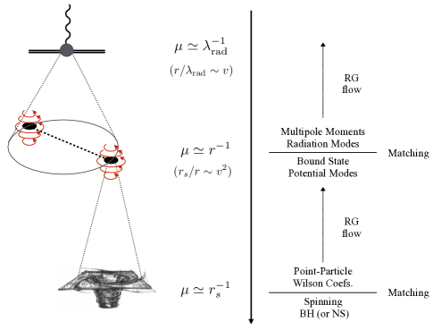
Figure 3: The EFT approach to the binary inspiral problem. See [16] for a thorough review.

3.1 The EFT framework: NRGR

The relevant scales for the binary inspiral problem are, the size of the compact object, $r_{s}$, the separation, $r$, and the typical wavelength of the emitted radiation, $\lambda_{\rm rad}\sim r/v$. For a bound state we also have $r_{s}/r\sim v^{2}$, and therefore

$$r_{s}\ll r\ll\lambda_{\rm rad}\,,$$ (3.1)

in the PN regime, $v\ll 1$. Therefore, after the hard scale, $r_{s}$, is integrated out we encounter two relevant regions for the binary problem (recall soft modes are not present in classical computations). Namely, the –off-shell– potential,

$$(p^{0}_{\rm pot},{\bm{p}}_{\rm pot})\sim(v/r,1/r)\,,$$ (3.2)

and –on-shell– radiation (or ultra-soft) modes,

$$(p^{0}_{\rm rad},{\bm{p}}_{\rm rad})\sim(v/r,v/r)\,.$$ (3.3)

The NRGR action takes the form ($L=i_{i}\ldots i_{\ell}$)

$${}S_{\rm NRGR}[x^{(p)}_{\rm cm}(\tau),h_{\mu\nu}] = \sum_{p}\int d\tau_{p}\left[-M_{(p)}(\tau)-\frac{1}{2}\omega_{\mu\,ab}S_{(p)}^{ab}(\tau)u^{\mu}(\tau)\right.$$ (3.4)

$$+ \left.\sum_{\ell=2}\left(\frac{1}{\ell!}I_{{\rm src}(p)}^{L}(\tau)\nabla_{L-2}E_{i_{\ell-1}i_{\ell}}-\frac{2\ell}{(2\ell+1)!}J_{{\rm src}(p)}^{L}(\tau)\nabla_{L-2}B_{i_{\ell-1}i_{\ell}}\right)\right]\,,$$

where $x^{(p)}_{\rm cm}(\tau)$ is the center-of-mass worldline of the bodies, $\omega_{\mu\,ab}$ are the Ricci coefficients, and $E_{ij}$, $B_{ij}$ are the electric and magnetic components of the Weyl tensor. The metric perturbation, $h_{\mu\nu}=g_{\mu\nu}-\eta_{\mu\nu}$, has support on modes longer than the hard scale, and it includes both potential and radiation modes. The monopole, $M$, represents the mass, $S_{ab}$ is the spin tensor, and the $I^{L}_{\rm src},J^{L}_{\rm src}$ are the permanent mass- and current-type source multipole moments, of the compact objects [16].

The EFT for at the radiation scale is constructed similarly to pNRQED (although at the non-linear level the structure resembles pNRQCD instead), by integrating out the potential modes [16]. Unlike QED, all the calculations remain at the classical level, involving a series of iterations of Green’s functions convoluted with external sources. Because of the symmetries of the long-distance theory, i.e. general relativity, the effective action in the radiation sector is exactly the same as in (3.4), but only radiation fields are present. The bodies are replaced by a single worldline at the center-of-mass of the binary, and the Wilson coefficients are now associated with the two-body system. For example, $M$ is the (Bondi) binding energy of the bound state, and $(I^{L}_{\rm src},J^{L}_{\rm src})$ are the corresponding source multipole moments. In principle, the power loss is obtained in terms of their time derivatives, using the equations of motion which follow from the gravitational binding potential [16]. See fig. 3 for a schematic representation of the relevant scales in NRGR. There is yet one other important contribution to be considered, namely the tail effect, or the scattering of the outgoing radiation off of the Newtonian potential produced by the whole binary. This is responsible for the rich structure of the radiation theory [24, 63, 28].

3.2 The tail effect

Figure 4: The tail contribution to the radiative quadrupole moment. Only the lines with an arrow propagate. The double-line represents the two-body system, treated as an external non-propagating source.

The interaction of the binary’s gravitational potential with the outgoing radiation modifies the total emitted power. In practice, the source moments, $I^{L}_{\rm src}$, which enter in the effective action in (3.4), turn into radiative multipoles, $I^{L}_{\rm rad}$, in the computation of the radiated power [6]. For example, the radiative quadrupole is obtained by computing the Feynman graph in fig. 4, which follows from the interaction between the quadrupole, $I_{\rm src}^{ij}$, and the monopole, $M$. The calculation is straightforward, and one obtains a correction of the form [24, 64, 65, 66],

$$I^{ij}_{\rm rad}(\omega)=I^{ij}_{\rm src}(\omega)\left[1+GM\omega\left({\rm sign}(\omega)\pi+i\left[\frac{2}{\epsilon_{\rm IR}}+\log\omega^{2}/\mu^{2}+{\rm finite}\right]\right)\right]\,,$$ (3.5)

which features an IR divergence. It is easy to see all the IR poles cancel out in the radiated power, since they add up to an overall phase [24]. (This type of IR divergence is thus intimately related to the soft factors in QED [47].) However, similarly to what occurred for the Lamb shift, the contribution from the tail effect to radiation-reaction, and in particular its conservative part, features instead a UV divergence, see fig. 5,

$$\int dt\,V_{\rm tail}(\mu)=\,\frac{G_{N}^{2}M}{5}\int\frac{d\omega}{2\pi}\,\omega^{6}\,I_{\rm src}^{ij}(-\omega)I_{\rm src}^{ij}(\omega)\left[\frac{1}{\epsilon_{\rm UV}}+\log\frac{\omega^{2}}{\mu^{2}}+{\rm finite}\right].$$ (3.6)

(We drop the ‘src’ label below since all the multipole moments in what follows refer to the source.) The term in (3.6) is the equivalent to (2.3) in the derivation of the Lamb shift. By the same token, the IR divergence in the NRGR potential from the near region (which enters as a local term in the radiation theory) is the analogous to the one in (2.16), through (2.12). All we need is to show that the coefficients of the poles (and the $\log\mu^{2}$) match, as they do in NRQED.While the computation of the 4PN gravitational potential within the EFT approach is still undergoing [26, 27], we expect to find the following structure in the near region [28, 39]

$$\int dt\,V_{\rm pot}(\mu)=-\frac{G_{N}^{2}M}{5}\int\frac{d\omega}{2\pi}\omega^{6}I^{ij}(-\omega)I^{ij}(\omega)\left(\frac{1}{\epsilon_{\rm IR}}-2\log(\mu r)\right)+{\rm local/finite}\,.$$ (3.7)

Hence, adding both contributions together, and restricting to a circular orbit (for which $\omega\simeq 2v/r$), we would get [28] (see fig. 6)

$$V_{\rm full}=V_{\rm pot}+V_{\rm tail}=\frac{2G_{N}^{2}M}{5}I^{ij(3)}(t)I^{ij(3)}(t)\left[\log v+\frac{1}{2}\left(\frac{1}{\epsilon_{\rm UV}}-\frac{1}{\epsilon_{\rm IR}}\right)\right]+{\rm finite}\,.$$ (3.8)

The uperscript $(n)$ represents the $n$-th time derivative. In [39] we elaborate on the zero-bin prescription to deal with the divergences in (3.8), which are the source of ambiguities in the regularization schemes implemented in [31, 32, 33, 34, 35, 36, 37]. The logarithmic correction, on the other hand, is universal [28]. The latter may be obtained unambiguously without the need of any matching condition, as we show next.

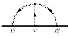
Figure 5: The tail contribution to radiation-reaction. The $(+,-)$ labels are associated to the ‘in-in’ formalism, required to properly compute retardation effects. The wavy line is a radiation mode $p^{\mu}\sim\lambda_{\rm rad}^{-1}$, whereas the dashed line corresponds to a potential mode with ${\bm{q}}\sim\lambda_{\rm rad}^{-1}$. See [28] for more details.

3.3 The renormalization group

As we did for the Lamb shift, let us proceed from the bottom up, where the gravitational potential from the near zone becomes a matching coefficient in the far zone. Therefore, as before (see e.g. (2.48)), we split the local contribution from the near region into a renormalized part and a counter-term. The latter is chosen to renormalize the –conservative– contribution from the tail effect [28]

$$V_{\rm c.t.}=-\frac{G_{N}^{2}M}{5}I^{ij(3)}(t)I^{ij(3)}(t)\frac{1}{\epsilon_{\rm UV}},$$ (3.9)

so that we end up with a full gravitational potential of the form

$$V_{\rm full}=V_{\rm ren}(\mu)+\frac{G_{N}^{2}M}{5}\int\frac{d\omega}{2\pi}\,\omega^{6}\,I^{ij}(-\omega)I^{ij}(\omega)\left[\log\frac{\omega^{2}}{\mu^{2}}+{\rm finite}\right].$$ (3.10)

This expression is similar to (2.54). Hence, by demanding the $\mu$-independence of the (physical) gravitational potential [28] we find,

$$\mu\frac{d}{d\mu}V_{\rm full}=0\to\mu\frac{d}{d\mu}V_{\rm ren}(\mu)=\frac{2G_{N}^{2}M}{5}I^{ij(3)}(t)I^{ij(3)}(t)\,,$$ (3.11)

which is the equivalent of (2.51). Once again, considering a circular orbit and choosing $\mu\sim v/r$, the renormalization group equation carries the information about the logarithmic contribution,

$$V_{\rm full}^{\rm\log}=\frac{2G_{N}^{2}M}{5}I^{ij(3)}(t)I^{ij(3)}(t)\log v\,,$$ (3.12)

reproducing (3.8). From here, following the step described in [28], we derived the logarithm entering in the (conserved) binding energy at 4PN order,

$$E_{\rm log}=-2G_{N}^{2}M\big{\langle}I^{ij(3)}(t)I^{ij(3)}(t)\big{\rangle}\log v\,,$$ (3.13)

which agrees with the result in [67].

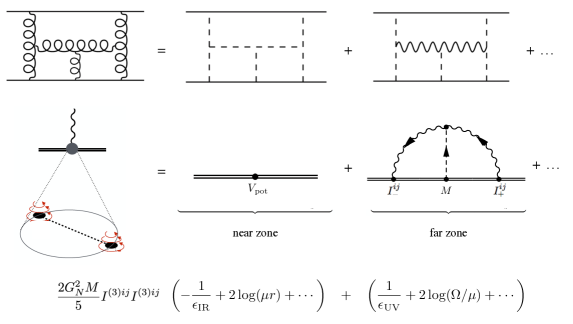
Figure 6: The full theory computation in general relativity (curly propagators) is split into regions in the EFT formalism: potential (dashed) and radiation (wavy) modes. The subsequent IR/UV divergences appear from the splitting into near and far zones [28]. The calculations are similar to the derivation of the (quantum) Lamb shift described here, except that the gravitational case involves non-linear couplings (and is fully classical). The logarithmic contribution, scaling as $Mv^{8}\log v$, resembles Bethe logarithm in electrodynamics.

4 Concluding remarks

In this paper we studied the Lamb shift using NRQED, illustrating an ambiguity-free derivation of the binding energy within an EFT framework. The parallel with the gravitational case was already emphasized in [31, 32], quote: “It is worth pointing out that also the Lamb shift calculation of Ref. [54] shows up an undefined constant in the IR sector, which gets fixed by some dimensional matching.” Indeed, an IR singularity appears in the near zone calculations in NRQED, resembling the situation in gravity. Likewise, a UV pole arises from an ultra-soft loop in the far region, echoing the calculation of the (conservative part of) the tail effect in NRGR [28]. Yet, as we showed, the IR/UV divergences in the Lamb shift can be removed without the need to introduce ambiguities. The procedure is implemented for NRGR in [39]. We also rederived the renormalization group equations from which we reproduce both logarithmic contributions, to the –quantum– shift in the energy levels of the Hydrogen atom and the –classical– gravitational binding potential for binary black holes.

References

- [1] Virgo, LIGO Scientific Collaboration, J. Abadie et al., “Predictions for the Rates of Compact Binary Coalescences Observable by Ground-based Gravitational-wave Detectors,” Class. Quant. Grav. 27 (2010) 173001, arXiv:1003.2480 [astro-ph.HE].
- [2] Virgo, LIGO Scientific Collaboration, B. P. Abbott et al., “Observation of Gravitational Waves from a Binary Black Hole Merger,” Phys. Rev. Lett. 116 no. 6, (2016) 061102, arXiv:1602.03837 [gr-qc].
- [3] A. Sesana, “Prospects for Multiband Gravitational-Wave Astronomy after GW150914,” Phys. Rev. Lett. 116 no. 23, (2016) 231102, arXiv:1602.06951 [gr-qc].
- [4] Virgo, LIGO Scientific Collaboration, B. P. Abbott et al., “Astrophysical Implications of the Binary Black-Hole Merger GW150914,” Astrophys. J. 818 no. 2, (2016) L22, arXiv:1602.03846 [astro-ph.HE].
- [5] Virgo, LIGO Scientific Collaboration, B. P. Abbott et al., “Binary Black Hole Mergers in the first Advanced LIGO Observing Run,” Phys. Rev. X6 no. 4, (2016) 041015, arXiv:1606.04856 [gr-qc].
- [6] L. Blanchet, “Gravitational Radiation from Post-Newtonian Sources and Inspiralling Compact Binaries,” Living Rev.Rel. 17 (2014) 2, arXiv:1310.1528 [gr-qc].
- [7] A. Buonanno and B. S. Sathyaprakash, “Sources of Gravitational Waves: Theory and Observations,” arXiv:1410.7832 [gr-qc].
- [8] A. Le Tiec, “The Overlap of Numerical Relativity, Perturbation Theory and Post-Newtonian Theory in the Binary Black Hole Problem,” Int. J. Mod. Phys. D23 no. 10, (2014) 1430022, arXiv:1408.5505 [gr-qc].
- [9] W. D. Goldberger and I. Z. Rothstein, “An Effective field theory of gravity for extended objects,” Phys.Rev. D73 (2006) 104029, arXiv:hep-th/0409156 [hep-th].
- [10] R. A. Porto, “Post-Newtonian corrections to the motion of spinning bodies in NRGR,” Phys.Rev. D73 (2006) 104031, arXiv:gr-qc/0511061 [gr-qc].
- [11] W. D. Goldberger, “Les Houches lectures on effective field theories and gravitational radiation,” 2007. arXiv:hep-ph/0701129 [hep-ph].
- [12] R. A. Porto and R. Sturani, “Scalar gravity: Post-Newtonian corrections via an effective field theory approach,” in Les Houches Summer School - Session 86: Particle Physics and Cosmology: The Fabric of Spacetime Les Houches, France, July 31-August 25, 2006. 2007. arXiv:gr-qc/0701105 [gr-qc].
- [13] I. Z. Rothstein, “Progress in effective field theory approach to the binary inspiral problem,” Gen. Rel. Grav. 46 (2014) 1726.
- [14] V. Cardoso and R. A. Porto, “Analytic approximations, perturbation theory, effective field theory methods and their applications,” Gen. Rel. Grav. 46 (2014) 1682, arXiv:1401.2193 [gr-qc].
- [15] S. Foffa and R. Sturani, “Effective field theory methods to model compact binaries,” Class. Quant. Grav. 31 no. 4, (2014) 043001, arXiv:1309.3474 [gr-qc].
- [16] R. A. Porto, “The effective field theorist’s approach to gravitational dynamics,” Phys. Rept. 633 (2016) 1–104, arXiv:1601.04914 [hep-th].
- [17] R. A. Porto and I. Z. Rothstein, “The Hyperfine Einstein-Infeld-Hoffmann potential,” Phys.Rev.Lett. 97 (2006) 021101, arXiv:gr-qc/0604099 [gr-qc].
- [18] R. A. Porto and I. Z. Rothstein, “Spin(1)Spin(2) Effects in the Motion of Inspiralling Compact Binaries at Third Order in the Post-Newtonian Expansion,” Phys.Rev. D78 (2008) 044012, arXiv:0802.0720 [gr-qc].
- [19] R. A. Porto and I. Z. Rothstein, “Next to Leading Order Spin(1)Spin(1) Effects in the Motion of Inspiralling Compact Binaries,” Phys.Rev. D78 (2008) 044013, arXiv:0804.0260 [gr-qc].
- [20] J. B. Gilmore and A. Ross, “Effective field theory calculation of second post-Newtonian binary dynamics,” Phys. Rev. D78 (2008) 124021, arXiv:0810.1328 [gr-qc].
- [21] S. Foffa and R. Sturani, “Effective field theory calculation of conservative binary dynamics at third post-Newtonian order,” Phys. Rev. D84 (2011) 044031, arXiv:1104.1122 [gr-qc].
- [22] R. A. Porto, “Next to leading order spin-orbit effects in the motion of inspiralling compact binaries,” Class.Quant.Grav. 27 (2010) 205001, arXiv:1005.5730 [gr-qc].
- [23] R. A. Porto, A. Ross, and I. Z. Rothstein, “Spin induced multipole moments for the gravitational wave flux from binary inspirals to third Post-Newtonian order,” JCAP 1103 (2011) 009, arXiv:1007.1312 [gr-qc].
- [24] W. D. Goldberger and A. Ross, “Gravitational radiative corrections from effective field theory,” Phys. Rev. D81 (2010) 124015, arXiv:0912.4254 [gr-qc].
- [25] A. Ross, “Multipole expansion at the level of the action,” Phys. Rev. D85 (2012) 125033, arXiv:1202.4750 [gr-qc].
- [26] S. Foffa and R. Sturani, “Dynamics of the gravitational two-body problem at fourth post-Newtonian order and at quadratic order in the Newton constant,” Phys. Rev. D87 no. 6, (2013) 064011, arXiv:1206.7087 [gr-qc].
- [27] S. Foffa, P. Mastrolia, R. Sturani, and C. Sturm, “Effective field theory approach to the gravitational two-body dynamics, at fourth post-Newtonian order and quintic in the Newton constant,” arXiv:1612.00482 [gr-qc].
- [28] C. R. Galley, A. K. Leibovich, R. A. Porto, and A. Ross, “Tail effect in gravitational radiation reaction: Time nonlocality and renormalization group evolution,” Phys. Rev. D93 (2016) 124010, arXiv:1511.07379 [gr-qc].
- [29] M. Levi and J. Steinhoff, “Next-to-next-to-leading order gravitational spin-orbit coupling via the effective field theory for spinning objects in the post-Newtonian scheme,” JCAP 1601 (2016) 011, arXiv:1506.05056 [gr-qc].
- [30] M. Levi and J. Steinhoff, “Next-to-next-to-leading order gravitational spin-squared potential via the effective field theory for spinning objects in the post-Newtonian scheme,” JCAP 1601 (2016) 008, arXiv:1506.05794 [gr-qc].
- [31] P. Jaranowski and G. Schafer, “Dimensional regularization of local singularities in the 4th post-Newtonian two-point-mass Hamiltonian,” Phys. Rev. D87 (2013) 081503, arXiv:1303.3225 [gr-qc].
- [32] P. Jaranowski and G. Schafer, “Derivation of the local-in-time fourth post-Newtonian ADM Hamiltonian for spinless compact binaries,” arXiv:1508.01016 [gr-qc].
- [33] T. Damour, P. Jaranowski, and G. Schafer, “Nonlocal-in-time action for the fourth post-Newtonian conservative dynamics of two-body systems,” Phys. Rev. D89 no. 6, (2014) 064058, arXiv:1401.4548 [gr-qc].
- [34] T. Damour, P. Jaranowski, and G. Schafer, “Conservative dynamics of two-body systems at the fourth post-Newtonian approximation of general relativity,” Phys. Rev. D93 no. 8, (2016) 084014, arXiv:1601.01283 [gr-qc].
- [35] L. Bernard, L. Blanchet, A. Bohe, G. Faye, and S. Marsat, “Fokker action of nonspinning compact binaries at the fourth post-Newtonian approximation,” Phys. Rev. D93 no. 8, (2016) 084037, arXiv:1512.02876 [gr-qc].
- [36] L. Bernard, L. Blanchet, A. Bohe, G. Faye, and S. Marsat, “Energy and periastron advance of compact binaries on circular orbits at the fourth post-Newtonian order,” Phys. Rev. D95 (2017) 044026, arXiv:1610.07934 [gr-qc].
- [37] T. Damour and P. Jaranowski, “Four-loop static contribution to the gravitational interaction potential of two point masses,” Phys. Rev. D95 no. 8, (2017) 084005, arXiv:1701.02645 [gr-qc].
- [38] L. Blanchet and A. Le Tiec, “First Law of Compact Binary Mechanics with Gravitational-Wave Tails,” arXiv:1702.06839 [gr-qc].
- [39] R. A. Porto and I. Z. Rothstein, “On the Apparent Ambiguities in the Post-Newtonian Expansion for Binary Systems,” arXiv:1703.06433 [gr-qc].
- [40] W. E. Lamb and R. C. Retherford, “Fine Structure of the Hydrogen Atom by a Microwave Method,” Phys. Rev. 72 (1947) 241–243.
- [41] H. A. Bethe, “The Electromagnetic shift of energy levels,” Phys. Rev. 72 (1947) 339.
- [42] F. J. Dyson, “The Electromagnetic shift of energy levels,” Phys. Rev. 73 (1948) 617.
- [43] J. B. French and V. F. Weisskopf, “The Electromagnetic shift of energy levels,” Phys. Rev. 75 (1949) 1240.
- [44] N. M. Kroll and W. E. Lamb, “On the Self-Energy of a Bound Electron,” Phys. Rev. 75 (1949) 388.
- [45] A. V. Manohar and I. W. Stewart, “The Zero-Bin and Mode Factorization in Quantum Field Theory,” Phys. Rev. D76 (2007) 074002, arXiv:hep-ph/0605001 [hep-ph].
- [46] A. V. Manohar, “The HQET / NRQCD Lagrangian to order alpha /m-3,” Phys. Rev. D56 (1997) 230–237, arXiv:hep-ph/9701294 [hep-ph].
- [47] S. Weinberg, “Infrared photons and gravitons,” Phys. Rev. 140 (1965) B516–B524.
- [48] M. Beneke and V. A. Smirnov, “Asymptotic expansion of Feynman integrals near threshold,” Nucl. Phys. B522 (1998) 321–344, arXiv:hep-ph/9711391 [hep-ph].
- [49] H. W. Griesshammer, “Threshold expansion and dimensionally regularized NRQCD,” Phys. Rev. D58 (1998) 094027, arXiv:hep-ph/9712467 [hep-ph].
- [50] B. Grinstein and I. Z. Rothstein, “Effective field theory and matching in nonrelativistic gauge theories,” Phys. Rev. D57 (1998) 78–82, arXiv:hep-ph/9703298 [hep-ph].
- [51] W. E. Caswell and G. P. Lepage, “Effective Lagrangians for Bound State Problems in QED, QCD, and Other Field Theories,” Phys. Lett. B167 (1986) 437–442.
- [52] N. Brambilla, A. Pineda, J. Soto, and A. Vairo, “Potential NRQCD: An Effective theory for heavy quarkonium,” Nucl. Phys. B566 (2000) 275, arXiv:hep-ph/9907240 [hep-ph].
- [53] I. Z. Rothstein, “TASI lectures on effective field theories,” arXiv:hep-ph/0308266 [hep-ph].
- [54] L. S. Brown, Quantum field theory. Cambridge University Press, 1994.
- [55] L. S. Brown, “New use of dimensional continuation illustrated by dE/dx in a plasma and the Lamb Shift,” Phys. Rev. D62 (2000) 045026, arXiv:physics/9911056 [physics].
- [56] A. Pineda and J. Soto, “The Lamb shift in dimensional regularization,” Phys. Lett. B420 (1998) 391–396, arXiv:hep-ph/9711292 [hep-ph].
- [57] J. Schwinger, “Coulomb Green’s Function,” J. Math. Phys. 5 (1964) 1606–1608.
- [58] M. E. Luke, A. V. Manohar, and I. Z. Rothstein, “Renormalization group scaling in nonrelativistic QCD,” Phys. Rev. D61 (2000) 074025, arXiv:hep-ph/9910209 [hep-ph].
- [59] A. V. Manohar and I. W. Stewart, “Logarithms of alpha in QED bound states from the renormalization group,” Phys. Rev. Lett. 85 (2000) 2248–2251, arXiv:hep-ph/0004018 [hep-ph].
- [60] A. H. Hoang, A. V. Manohar, and I. W. Stewart, “The Running Coulomb potential and Lamb shift in QCD,” Phys. Rev. D64 (2001) 014033, arXiv:hep-ph/0102257 [hep-ph].
- [61] R. A. Porto, “The Tune of Love and the Nature(ness) of Spacetime,” Fortsch. Phys. 64 no. 10, (2016) 723–729, arXiv:1606.08895 [gr-qc].
- [62] V. Cardoso, E. Franzin, A. Maselli, P. Pani, and G. Raposo, “Testing strong-field gravity with tidal Love numbers,” Phys. Rev. D95 no. 8, (2017) 084014, arXiv:1701.01116 [gr-qc]. [Addendum: Phys. Rev.D95,no.8,089901(2017)].
- [63] W. D. Goldberger, A. Ross, and I. Z. Rothstein, “Black hole mass dynamics and renormalization group evolution,” Phys. Rev. D89 no. 12, (2014) 124033, arXiv:1211.6095 [hep-th].
- [64] R. A. Porto, A. Ross, and I. Z. Rothstein, “Spin induced multipole moments for the gravitational wave amplitude from binary inspirals to 2.5 Post-Newtonian order,” JCAP 1209 (2012) 028, arXiv:1203.2962 [gr-qc].
- [65] L. Blanchet and T. Damour, “Hereditary effects in gravitational radiation,” Phys. Rev. D46 (1992) 4304–4319.
- [66] L. Blanchet, “Time asymmetric structure of gravitational radiation,” Phys. Rev. D47 (1993) 4392–4420.
- [67] L. Blanchet, S. L. Detweiler, A. Le Tiec, and B. F. Whiting, “High-Order Post-Newtonian Fit of the Gravitational Self-Force for Circular Orbits in the Schwarzschild Geometry,” Phys. Rev. D81 (2010) 084033, arXiv:1002.0726 [gr-qc].