Abstract

The goal in semi-supervised learning is to effectively combine labeled and unlabeled data. One way to do this is by encouraging smoothness across edges in a graph whose nodes correspond to input examples. In many graph-based methods, labels can be thought of as propagating over the graph, where the underlying propagation mechanism is based on random walks or on averaging dynamics. While theoretically elegant, these dynamics suffer from several drawbacks which can hurt predictive performance.

Our goal in this work is to explore alternative mechanisms for propagating labels. In particular, we propose a method based on dynamic infection processes, where unlabeled nodes can be “infected” with the label of their already infected neighbors. Our algorithm is efficient and scalable, and an analysis of the underlying optimization objective reveals a surprising relation to other Laplacian approaches. We conclude with a thorough set of experiments across multiple benchmarks and various learning settings.

1 Introduction

The supervised learning framework underlies much of the empirical success of machine learning systems. Nonetheless, results in unsupervised learning have demonstrated that there is much to be gained from unlabeled data as well. This has prompted considerable interest in the semi-supervised learning [11] setting, where the data includes both labeled and unlabeled examples. Methods for semi-supervised learning (SSL) are especially useful for applications in which unlabeled examples are ample, but labeled examples are scarce or expensive.

One of the most wide-spread approaches to SSL, and our focus in this paper, is the class of graph-based methods. In these, part of the problem input is a graph that specifies which input points should be considered close. Graph-based methods assume that proximity in the graph implies similarity in labels. There are many variations on this idea [5, 7, 37, 41], each using smoothness and graph distance differently. However, they all share the intuition that the classification function should be smooth with respect to the graph.

One way for encouraging smoothness is by optimizing an objective based on the graph Laplacian. This is prevalent in classic SSL methods such as Label Propagation (LabelProp) [47] and its variants [46, 4, 42], as well as in recent deep graph embedding methods [45, 36]. In some cases, the Laplacian objective can be interpreted as the probability that a random walk terminates at a certain state. In others, the objective can be expressed as a quadratic form which can be optimized by iterative local averaging of labels. The optimization process can hence be thought of as propagating labels under a certain averaging dynamic process, whose steady state corresponds to the optimum. Due to their elegance, computational properties, and empirical power, random walks and local averaging have become the standard mechanisms for propagating information in many applications. Nonetheless, they have several shortcomings, which we address here.

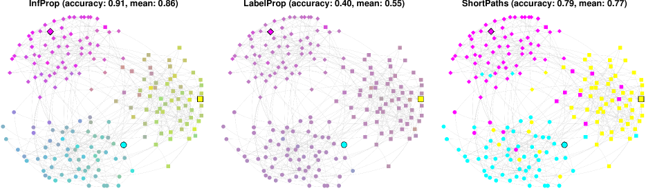
Figure 1: For graphs with weakly inter-connected components, infection dynamics (our method, left) propagate labels better than random walks (middle) or shortest paths (right). Labeled nodes are outlined, shapes denote true labels, and probabilistic predictions are encoded by CMY color values. See supp. material for more details.

First, many of the guarantees of such methods hold only for undirected graphs. For directed graphs, the Laplacian is not necessarily PSD, meaning that the objective is no longer convex, and that the quadratic smoothness interpretation breaks down. Optimization in directed graph Laplacians is much harder and far less understood [43], and sampling is computationally prohibitive, slow to converge, and unstable [29, 30].

Second, such methods were originally designed for graphs that approximate the density of the data in feature space. As such, they can fail when applied to real graphs, especially large networks with a community structure. This is because random walks are prone to get stuck in local neighborhoods [9], because visiting all nodes can require an expected $O(n^{3})$ steps [2], and since the limit distribution can be uninformative for large graphs [44] or when labels are rare [33].

Third, extending such methods beyond the vanilla multiclass setting has proven to be quite challenging. For instance, outputting confidence in predictions is possible, but leads to extremely low values [42]. Label priors can be utilized, but only in determining the classification rule, rather than being incorporated into the model [47]. Most methods for an active semi-supervised setting are either heuristic [23] or based on pessimistic worst-case objectives [24]. Finally, supporting structured labels is far from straightforward and can be computationally demanding [3].

Due to the above, in this work we advocate for considering alternative mechanisms for propagating labels over a graph, and propose an approach which addresses most of the above issues. Our method, called Infection Propagation (InfProp), views the process of labeling the graph as a dynamic infection process. Initially, only the labeled nodes are “infected” with their known labels. As time unfolds, infected nodes can, with some probability, infect their unlabeled neighbors. When this happens, the unlabeled nodes inherit the label of their infector. Labeled nodes can therefore be viewed as competing over infecting the unlabeled nodes with their labels. Since the infection process is stochastic, we can calculate the probability that a given node was infected by a given label, and label the node according to this probability.

InfProp is motivated by the idea that different graph types may require different dynamics for efficient propagation of information. It is inspired by propagation dynamics found in the natural and social worlds, and draws on the successful application of infection models in different contexts [26, 20, 14]. InfProp is especially efficient for graphs with highly intra-connected but lightly inter-connected components, a characteristic of many real-world networks. Fig. 1 illustrates this for a small synthetic random network with three clusters (see supplementary material for details). As can be seen, InfProp propagates information correctly, even when the seed set is very small. In comparison, LabelProp provides uninformative and almost uniform predictions which are prone to error, and shortest paths over the weighted graph err due to cross-cluster links.

InfProp uses infection probabilities for labeling; these, however, turn out to be #P hard to compute exactly. We therefore provide a fully polynomial-time randomized approximation scheme (FPRAS). Our solution exploits an equivalence between the infection process and shortest paths in random graphs. The resulting algorithm is easy to parallelize, making the method highly scalable. It also extends to various learning settings, such as multilabel prediction and active SSL.

In Sec. 5 we analyze the optimization objective underlying the propagation of labels via infection dynamics, highlighting an intriguing connection graph Laplacians. Our analysis shows that InfProp can be viewed as optimizing a quadratic objective, in which weights are seed-specific and related in an intricate manner to the underlying diffusion process. We conclude with an extensive set of experiments in multiple learning settings which demonstrate the effectiveness of our approach.

2 Propagating Labels with Infections

In this section we present our infection-based method for semi-supervised learning. We are given as input a directed weighted graph $G=(V,E,W)$, as well as a subset of labeled nodes ${S}\subseteq V$ referred to as the seed set. Each seed node $s\in{S}$ also comes with a true label $y_{s}\in{\mathcal{Y}}$. We denote the unlabeled nodes by ${U}=V\setminus{S}$, and set $n=|V|$, $m=|E|$, $L=|{\mathcal{Y}}|$, and $k=|{S}|$. In some settings additional node features are available. We focus on the transductive setting, where the goal is to predict the labels of all non-seed nodes $u\in{U}$.

The core idea of our method is to propagate labels from labeled to unlabeled nodes using infection dynamics. The process is initialized with all seed nodes in an infected state and all unlabeled nodes in a null state ${\varnothing}$. Then, a stochastic model of infection dynamics is used to determine how the infectious state of nodes in the graph changes over time, typically as a function of the states of neighboring nodes. To support multiple label classes, we consider competitive infection models. In these, seeds $s\in{S}$ are initially infected with their true labels $y_{s}$, and compete in infecting unlabeled nodes.

The models we consider are stochastic and converge to a steady state. This means that, after some time point, the labels of all nodes will not change anymore (we refer to this as process termination, or steady state). Since the process itself is stochastic, each instantiation will result in a different value for the labels at termination. For a given infection model, let ${Y}_{v\ell}$ be the binary random variable indicating whether node $v$ is infected by label $\ell$ at steady state. Since our goal is to reason about the labels of the nodes, it will be natural to utilize the infection dynamics to generate probabilistic predictions. For each node $v$, our method outputs a distribution over labels ${f}_{v}$. Each entry ${f}_{v\ell}$ corresponds to the probability that $v$ had value $\ell$ at steady state, as a function of the seed set ${S}$ and its labels:

$${f}_{v\ell}({S},y)=\mathbb{P}\left[{{Y}_{v\ell}=1}\right]=\mathbb{E}\left[{{Y}_{v\ell}}\right]$$ (1)

Note that $\ell$ can take values in $1,\ldots,L$ but also $\ell=0$ for ${\varnothing}$. The entry ${f}_{v0}$ therefore describes the (possibly non-negative) probability that $v$ remained uninfected.

Computing ${f}$ exactly is known to be #P-hard even for simple infection models [14]. Hence, like many other infection-based methods [26, 17, 16], we resort to a Monte-Carlo approach and estimate ${f}$ by averaging over infection outcomes ${Y}$. Our final predictor ${\hat{{f}}}$ is:

$${\hat{{f}}}_{v\ell}({S},y)=\frac{1}{N}\sum\nolimits_{i=1}^{N}{Y}^{(i)}_{v\ell}$$ (2)

where ${Y}^{(i)}_{v\ell}$ is an indicator for the $i^{\text{th}}$ random instance.

In principle, outcomes ${Y}$ can be evaluated by simulating the infection dynamics. This however is not straightforward for several of the models we consider, such as those with continuous time. In the next section we describe some infection models, and show how ${\hat{{f}}}$ can be efficiently computed for them using an alternative graphical representation of the infection process.

We conclude by stating an approximation bound for $f$. As we can calculate $\hat{f}$ efficiently (see next section) this implies that our method yields an efficient approximation scheme for the true infection probabilities.

Proposition 1.

For every $\epsilon,\,\delta\in[0,1]$, if $N\geq\frac{1}{2\epsilon^{2}}\log{\frac{2n(L+1)}{\delta}}$, then with probability of at least $1-\delta$, Algorithm 2 returns ${\hat{{f}}}$ such that $\|{\hat{{f}}}-{f}\|_{\max{}}\leq\epsilon$. thm:convergence

Proof.

Note that each ${Y}_{v\ell}$ is a random variable in $\{0,1\}$. Furthermore, ${\hat{{f}}}$ is an average of ${Y}$, and ${f}$ is the corresponding expectation. The result is obtained by applying the Hoeffding and union bounds. ∎

2.1 Competitive Infection Models for Graph Labeling

As mentioned above, our SSL method relies on an infection process where nodes of the graph are “infected” with labels. There are many variants of infection processes (see [13]); we describe some relevant ones below.

2.1.1 The Independent Cascade model

Since its introduction in [19], the simple but powerful Independent Cascade (IC) model has been used extensively. The original IC model, briefly reviewed below, is a discrete-time, network-dependent interpretation of the classic Susceptible-Infected-Recovered (SIR) epidemiological model [27]. At time $t=0$, seed nodes are initialized to an infected state, and all other nodes to a susceptible state. If node $u$ is infected at time step $t$, then at time $t+1$ it attempts to infect each of its non-infected out-neighbors $v\in{Nei({u})}$, and succeeds with probability $p_{uv}$. If successful, we refer to the edge $(u,v)$ as active or activated, mark the infection time of $v$ as $\tau_{v}=t+1$, and set $v$’s infector to be $u$, which we denote by ${\rho}(v)=u$. The model is therefore parametrized by the set of all edge infection probabilities $\{p_{uv}\,|\,(u,v)\in E\}$ (given as input via $p_{uv}=W_{uv}$). Once a node becomes infected, it remains in this state. As infections are probabilistic, not all nodes are necessarily infected. The process terminates either when all nodes are infected, or (more commonly) when all infection attempts at some time step are unsuccessful.

The IC model describes the propagation of a single infectious content. Hence, it can tell us only when and how a node is infected, but not by what. This motivated a class of competitive infection models which support multiple content types. Several competitive IC variants have been proposed [8, 10, 12, 25]. The common theme in these is that nodes inherit the label of their earliest infector (with tie-breaking when needed). All of these are supported by our method. In the supplementary material we show how our approach can also be applied to threshold models [26].

2.1.2 Continuous Time Dynamics

While simple and elegant, the IC dynamics are somewhat limited in their expressive power. One important generalization is the Continuous-Time IC model (CTIC) [20]. This model is well suited for SSL as it is flexible, does not require tie-breaking, and allows for incorporating node priors. In this model, a successful infection attempt entails an “incubation period”, after which the node becomes infected. Hence, if $u$ succeeds in infecting $v$ at time $\tau_{u}\in\mathbb{R}^{+}$, it draws an incubation time $\delta_{uv}\sim{D}(\theta_{uv})$, and $v$ can become infected at time $\tau_{uv}=\tau_{u}+\delta_{uv}$. As in the IC model, $v$ inherits the label of its earliest infector ${\rho}(v)=\operatorname*{argmin}_{u}\tau_{uv}$. The competitive CTIC model generalizes the competitive IC model for an appropriate choice of $D$, where $\delta_{e}$ is set to 1 with probability $p_{e}$, and $\infty$ with probability $1-p_{e}$. We therefore consider a general mixture distribution of activations and incubation times ${D}(p,\theta)$, where $\delta_{e}$ is sampled w.p. $p_{e}$, and set to $\infty$ w.p. $1-p_{e}$. Since infections are determined by the earliest successful attempt, the shortest-paths interpretation and algorithm (Sec. 2.2.1) hold for the random graph $G^{\delta}=(V,E,\delta)$.

2.2 Computing Infections Efficiently

For infection models as in Sec. 2.1, we would like to calculate predictions $\hat{f}$ as in Eq. (2). A naive approach would be to do this by simulating the infection process $N$ times and averaging. This, however, is inefficient for discrete-time IC, requires continuous time simulation for CTIC, and does not apply to general models. We hence provide an equivalent efficient alternative below.

Algorithm 1 BasicInfProp($G,{S},y,p,N$)

1:  for $i=1,\dots,N$ do

2:     Initialize $Y^{(i)}_{u\ell}\leftarrow 0$ for all $u\in{U},\,\ell\in{\mathcal{Y}}\cup{\varnothing}$

3:     for $(u,v)\in E$ do

4:        $W_{uv}\leftarrow 1$ with probability $p_{uv}$, and $\infty$ o.w.

5:     for $s\in{S}$ do

6:        ${\text{dist}}[s][\,\cdotp]\leftarrow{\textsc{Dijkstra}}(G,W,s)$

7:     for $u\in{U}$ do

8:        $Y^{(i)}_{u,{\alpha}(u)}\leftarrow 1$ where ${\alpha}(u)\in\operatorname*{argmin}_{s}{\text{dist}}[s][u]$

9:  Return ${\hat{{f}}}=\frac{1}{N}\sum_{i=1}^{N}Y^{(i)}$

2.2.1 Infections as Shortest Paths

We now present an alternative view of the sampling process, which facilitates efficient implementation and extensions. Consider first the discrete time IC process. For a single instantiation of the process, recall that if $u$ succeeded in infecting $v$, the edge $(u,v)$ is considered active. We use the set of active edges $A\subseteq E$ (sampled throughout the instantiation until termination) to construct the active graph $G^{A}=(V,E,W^{A})$ with weights $W^{A}_{e}=1$ for $e\in A$ and $W^{A}_{e}=\infty$ for $e\in E\setminus A$. An important observation is that node $v$ is infected at termination iff there exists a path in $G^{A}$ from some seed node $s\in{S}$ to $v$ with finite weight. We refer to this as an active path. Since $v$’s actual infection time $\tau_{v}$ is set by the earliest successful infection, it is also the length of the shortest active path from some $s\in{S}$.

The above formulation allows for replacing time with graph distances. Let $d_{A}(u,v)$ be the distance from $u$ to $v$ in $G^{A}$. Due to the recursive nature of label assignment, it follows that $v$ inherits its label from the $s\in{S}$ whose distance to $v$ is shortest. We refer to $s$ as $v$’s ancestor, denoted by ${\alpha}(v)$, and set ${\alpha}(v)={\varnothing}$ when there are no paths from ${S}$ to $v$. Infection outcomes ${Y}_{v\ell}$ can now be expressed using distances:

$${Y}_{v\ell}={\mathds{1}}\{\ell=y_{{\alpha}(v)}\},\qquad{\alpha}(v)=\operatorname*{argmin}_{s\in{S}}d_{A}(s,v)$$ (3)

Recall that our motivation here was to compute $Y$ without simulating the dynamics. Since distances $d_{A}$ depend on edge activations, it is not yet clear why Eq. (3) is useful. An important result by [26] shows that ancestors can be computed over a simpler random graph model. Specifically, let ${\mathchoice{\accentset{\displaystyle\text{\smash{\raisebox{-5.59721pt}{$\widetildesym$}}}}{A}}{\accentset{\textstyle\text{\smash{\raisebox{-5.59721pt}{$\widetildesym$}}}}{A}}{\accentset{\scriptstyle\text{\smash{\raisebox{-3.91806pt}{$\widetildesym$}}}}{A}}{\accentset{\scriptscriptstyle\text{\smash{\raisebox{-2.7986pt}{$\widetildesym$}}}}{A}}}\subseteq E$ be a random edge set, where each edge $(u,v)\in E$ is sampled independently to be in ${\mathchoice{\accentset{\displaystyle\text{\smash{\raisebox{-5.59721pt}{$\widetildesym$}}}}{A}}{\accentset{\textstyle\text{\smash{\raisebox{-5.59721pt}{$\widetildesym$}}}}{A}}{\accentset{\scriptstyle\text{\smash{\raisebox{-3.91806pt}{$\widetildesym$}}}}{A}}{\accentset{\scriptscriptstyle\text{\smash{\raisebox{-2.7986pt}{$\widetildesym$}}}}{A}}}$ with probability $p_{uv}$. Then, for an appropriately defined $G^{{\mathchoice{\accentset{\displaystyle\text{\smash{\raisebox{-5.59721pt}{$\widetildesym$}}}}{A}}{\accentset{\textstyle\text{\smash{\raisebox{-5.59721pt}{$\widetildesym$}}}}{A}}{\accentset{\scriptstyle\text{\smash{\raisebox{-3.91806pt}{$\widetildesym$}}}}{A}}{\accentset{\scriptscriptstyle\text{\smash{\raisebox{-2.7986pt}{$\widetildesym$}}}}{A}}}}$ and $d_{{\mathchoice{\accentset{\displaystyle\text{\smash{\raisebox{-5.59721pt}{$\widetildesym$}}}}{A}}{\accentset{\textstyle\text{\smash{\raisebox{-5.59721pt}{$\widetildesym$}}}}{A}}{\accentset{\scriptstyle\text{\smash{\raisebox{-3.91806pt}{$\widetildesym$}}}}{A}}{\accentset{\scriptscriptstyle\text{\smash{\raisebox{-2.7986pt}{$\widetildesym$}}}}{A}}}}$, we have:

$${\alpha}(v)=\operatorname*{argmin}_{s\in{S}}d_{{\mathchoice{\accentset{\displaystyle\text{\smash{\raisebox{-5.59721pt}{$\widetildesym$}}}}{A}}{\accentset{\textstyle\text{\smash{\raisebox{-5.59721pt}{$\widetildesym$}}}}{A}}{\accentset{\scriptstyle\text{\smash{\raisebox{-3.91806pt}{$\widetildesym$}}}}{A}}{\accentset{\scriptscriptstyle\text{\smash{\raisebox{-2.7986pt}{$\widetildesym$}}}}{A}}}}(s,v)$$ (4)

Thus, to compute each ${Y}_{v\ell}^{(i)}$ (and hence ${\hat{{f}}}$), it suffices to sample edges independently, and compute shortest paths on $G^{{\mathchoice{\accentset{\displaystyle\text{\smash{\raisebox{-5.59721pt}{$\widetildesym$}}}}{A}}{\accentset{\textstyle\text{\smash{\raisebox{-5.59721pt}{$\widetildesym$}}}}{A}}{\accentset{\scriptstyle\text{\smash{\raisebox{-3.91806pt}{$\widetildesym$}}}}{A}}{\accentset{\scriptscriptstyle\text{\smash{\raisebox{-2.7986pt}{$\widetildesym$}}}}{A}}}}$, bypassing the need for simulation. Under this view, ${f}$ can be thought of as an ensemble of shortest-path predictors, whose weights are set by the dynamics. Algorithm 1 provides a simple implementation of this idea for the discrete time IC model. After sampling edges, the algorithm computes shortest paths (using Dikjstra) from each $s\in{S}$ to all $u\in{U}$. Then, each node $u$ is assigned the label of its ancestor ${\alpha}(u)$. This approach applies to a large class of infection models that admit to a similar graphical form [26].

2.2.2 Improved Efficiency via Modified Dijkstra

Recall that for a single infection instance, a node inherits its label from the closest seed node. Based on this, Algorithm 1 offers a direct approach for computing ${f}$, where shortest paths are computed from each of the $k$ seed nodes to every unlabeled node $v\in{U}$ using $k$ calls to Dijkstra. While correct, this method suffers an unnecessary factor of $k$ on its runtime. To reduce this overhead, we change Dijkstra’s initialization and updates, so that only a single call would suffice. Algorithm 2 implements this idea for the general CTIC model (Sec. 2.1.2) and allows for node priors (Sec. 2). The correctness of the algorithm is stated below, and a proof is provided in the supplementary material.

Proposition 2.

Algorithm 2 correctly computes the estimated infection probabilities ${\hat{{f}}}$ in Eq. (1). thm:correctness

The worst-case complexity of Dijkstra, and hence of each iteration in Algorithm 2, is $O(m+n\log n)$. Other implementations of Dijkstra which support further parallelization or GPUs [31] can also be modified for our setting. Nonetheless, the practical run time of Algorithm 2 can be, and typically is, much better, for two reasons. First, note that only the subset of active edges are traversed (and sampled on the fly), and only nodes which are reachable from ${S}$ are processed. The infection parameters $p$ therefore induce a tradeoff between the influence diameter of ${S}$ and the run time (empirical demonstration in Fig. 3 (left)). Second, many settings require “hard” predictions ${\hat{y}}\in{\mathcal{Y}}$, typically set by ${\hat{y}}_{v}=\operatorname*{argmax}_{\ell}{\hat{{f}}}_{u\ell}$. Hence, for ${\hat{y}}_{v}$ to be correct, it suffices that ${\hat{{f}}}_{u,y_{u}}\geq{\hat{{f}}}_{u\ell}$ for all $\ell\in{\mathcal{Y}}$, which does not require the full convergence stated in thm:convergence (empirical demonstration in Fig. 3 (right)).

In this section we showed how infection outcomes can be computed efficiently. It is therefore only natural to ask - what is it that infections optimize? In the next section we show that ${f}$ is in fact the solution to a quadratic optimization objective, whose weights intricately depend on the infection dynamics.

3 What do infections optimize?

Many SSL methods propose an optimization objective which encodes some notion of smoothness. For instance, the classic LabelProp algorithm [47] encourages adjacent nodes to agree on their predicted labels by minimizing a quadratic penalty term:

$$f_{\textsc{lp}}=\operatorname*{argmin}_{f^{\prime}}\sum_{\ell}\sum_{u,v}W_{uv}(f^{\prime}_{u\ell}-f^{\prime}_{v\ell})^{2}$$ (5)

for predictions ${f}^{\prime}$ and symmetric weights $W$, subject to ${f}^{\prime}_{s\ell}={{\mathds{1}}_{\{{\ell=y_{s}}\}}}$ for all $s\in{S}$. In this section we show that InfProp has a related interpretation. Specifically, we show that the InfProp predictions ${f}$ minimize the quadratic objective in Eq. (13).

Algorithm 2 InfProp ($G,{S},y,{D},{q},N$)

1:  for $i=1,\dots,N$ do

2:     Initialize $Y^{(i)}_{u\ell}\leftarrow 0$ for all $u\in{U},\,\ell\in{\mathcal{Y}}\cup{\varnothing}$

3:     for $v\in{U}$ do

4:        ${\text{dist}}[v]\leftarrow\infty,\,\,\,{\text{y}}[v]\leftarrow{\varnothing}$

5:     for $s\in{S}$ do

6:        ${\text{dist}}[s]\leftarrow 0,\,\,\,{\text{y}}[s]\leftarrow y_{s}$

7:        push $s$ into min-queue $Q$

8:     while $Q$ is not empty do

9:        pop $v$ from $Q$ $\triangleright$ break ties randomly

10:        for $u\in{Nei({v})}$ do

11:           sample $\delta_{vu}\sim D(\theta,p)$ $\triangleright$ incubation time

12:           if $\delta_{vu}=\infty$ then continue

13:           ${\text{alt}}\leftarrow{\text{dist}}[v]+w^{A}_{vu}+{q}_{u}({\text{y}}[v])$ $\triangleright$ penalize

14:           if ${\text{alt}}<{\text{dist}}[u]$ then

15:              ${\text{dist}}[u]={\text{alt}}$

16:              ${\text{y}}[u]\leftarrow{\text{y}}[v]$ $\triangleright$ $u$ inherits label from parent $v$

17:              push/update $u$ in $Q$ with ${\text{dist}}[u]$

18:     $Y^{(i)}_{u,{\text{y}}[v]}\leftarrow 1$ for all $u\in{U}$

19:  Return ${\hat{{f}}}=\frac{1}{N}\sum_{i=1}^{N}Y^{(i)}$

While similar in structure, the fundamental difference between Eqs. (5) and (13) lies in how the weights are determined. In LabelProp (and variants), edge weights are given as input, and are typically set according to some feature-based similarity measure. In this sense, each $W_{uv}$ is a local function of the features of $u$ and $v$. In contrast, weights in Eq. (13) are set in a global manner. As we show next, each weight is a function of the infection dynamics, of the specific seed set ${S}$, and, if available, of the features of all nodes. To demonstrate this, and to see why Eq. (13) holds, it will be helpful to analyze InfProp from a spectral perspective.

3.1 A Laplacian Interpretation for InfProp

An interesting property of LabelProp is that its objective can be expressed via the graph Laplacian. For a directed weighted graph, the normalized Laplacian is:

$${\mathcal{L}}_{\textsc{lp}}=I-\mathchoice{\accentset{\displaystyle\text{\smash{\raisebox{-5.59721pt}{$\widetildesym$}}}}{W}}{\accentset{\textstyle\text{\smash{\raisebox{-5.59721pt}{$\widetildesym$}}}}{W}}{\accentset{\scriptstyle\text{\smash{\raisebox{-3.91806pt}{$\widetildesym$}}}}{W}}{\accentset{\scriptscriptstyle\text{\smash{\raisebox{-2.7986pt}{$\widetildesym$}}}}{W}}$$ (6)

where $\mathchoice{\accentset{\displaystyle\text{\smash{\raisebox{-5.59721pt}{$\widetildesym$}}}}{W}}{\accentset{\textstyle\text{\smash{\raisebox{-5.59721pt}{$\widetildesym$}}}}{W}}{\accentset{\scriptstyle\text{\smash{\raisebox{-3.91806pt}{$\widetildesym$}}}}{W}}{\accentset{\scriptscriptstyle\text{\smash{\raisebox{-2.7986pt}{$\widetildesym$}}}}{W}}=D^{-1}W$, $D$ is diagonal with $D_{uu}=\sum_{v}W_{uv}$ (and $W$ is symmetric). The output of LabelProp can be computed by solving the system ${\mathcal{L}}_{\textsc{lp}}{f}^{\prime}=0$ for the unlabeled nodes. We now show that the infection-based predictions of InfProp also correspond to the solution of a certain Laplacian system which is determined by the seed set and the infection dynamics.

Consider a single infection instance, and denote by ${T}_{uv}({S})$ the random variable indicating whether $u$ was infected by $v$ for seed ${S}$, namely ${T}_{uv}({S})={{\mathds{1}}_{\{{u={\rho}(v)}\}}}$. We refer to the matrix ${T}$ as the infector matrix. Further denote by ${\bm{{T}}}$ the expected infector matrix ${\bm{{T}}}({S})=\mathbb{E}\left[{{T}({S})}\right]$. We use this to define the following Laplacian:

$${\mathcal{L}}({S})_{\vphantom{}}=I-{\bm{{T}}}({S})$$ (7)

Note that ${\mathcal{L}}_{\vphantom{}}$ is defined over the same graph $G$, but need not be symmetric. We now show that ${\mathcal{L}}$ is indeed a Laplacian matrix, and that it can be used to infer ${f}$.

Lemma 1.

thm:lap_nonhom The infection-based predictions ${f}_{\vphantom{}}$ in Eq. (2) are also the solution to the Laplacian system:

$${\mathcal{L}}({S})_{\vphantom{}}{f}={\bm{b}}({S})$$ (8)

where:

$${\bm{b}}_{u\ell}({S})=\sum_{v}b_{vu\ell}^{({S})},\qquad b_{vu\ell}^{({S})}=\text{cov}\left[{{T}_{vu}({S}),Y_{u\ell}}\right]$$

For conciseness, we defer the full proof to the supplementary material, and show here a useful special case.

Lemma 2.

thm:lap_hom If ${T}$ and $Y$ are uncorrelated, then the infection-based predictions ${f}_{\vphantom{}}$ in Eq. (2) are also the solution to the homogeneous Laplacian system:

$${\mathcal{L}}_{{\vphantom{}}}({S})f=0$$ (9)

Proof.

We first show that ${\mathcal{L}}$ is a graph Laplacian, namely that the sum of each row in ${\bm{{T}}}$ is equal to the corresponding diagonal element in $I$, which is 1. Since rows in ${T}$ have only one non-zero entry of value one, each row in ${\bm{{T}}}$ is positive and sums to one. Note that ${\bm{{T}}}_{u\cdotp}$ provides a distribution over the infectors of $u$.

We now prove Eq. (9). By definition, the label of each node at steady state is set to be that of its infector, namely $Y_{v\ell}=Y_{{\rho}(v),\ell}$ for all $v$ and $\ell$, or simply $Y=TY$. Using Eq. (2) and applying expectation, we have:

$${f}({S})_{\vphantom{}}=\mathbb{E}\left[{Y}\right]=\mathbb{E}\left[{{T}({S})Y}\right]$$ (10)

When ${T},Y$ are uncorrelated, $\mathbb{E}\left[{{T}Y}\right]=\mathbb{E}\left[{{T}}\right]\mathbb{E}\left[{Y}\right]$, hence ${f}_{\vphantom{}}={\bm{{T}}}{f}_{\vphantom{}}$. Rearranging concludes our proof. ∎

3.2 InfProp as Optimization

We next use the Laplacian insight above to provide an objective minimized by the InfProp solution. Begin by noting that for LabelProp, the solution of Eq. (6) coincides with the solution of the following objective:

$${f}_{\textsc{lp}} =\operatorname*{argmin}_{f^{\prime}}\|{\mathcal{L}}_{\textsc{lp}}f^{\prime}\|_{F}^{2}$$

$$=\operatorname*{argmin}_{f^{\prime}}\sum_{\ell}\sum_{u}\Big{(}f^{\prime}_{u\ell}-\sum_{v}\mathchoice{\accentset{\displaystyle\text{\smash{\raisebox{-5.59721pt}{$\widetildesym$}}}}{W}}{\accentset{\textstyle\text{\smash{\raisebox{-5.59721pt}{$\widetildesym$}}}}{W}}{\accentset{\scriptstyle\text{\smash{\raisebox{-3.91806pt}{$\widetildesym$}}}}{W}}{\accentset{\scriptscriptstyle\text{\smash{\raisebox{-2.7986pt}{$\widetildesym$}}}}{W}}_{uv}{f}^{\prime}_{v\ell}\Big{)}^{2}$$ (11)

where minimization is only over the unlabeled nodes, and $\|\cdotp\|_{F}$ denotes the Frobenius norm. This gives an alternative quadratic objective which bounds Eq. (5) and directly expresses the steady-state of LabelProp’s averaging dynamics. In a similar fashion, we can derive an equivalent formulation of $f$ in Eq. (8) via:

$${f}({S})=\operatorname*{argmin}_{f^{\prime}}\|{\mathcal{L}}({S})_{\vphantom{}}f^{\prime}-{\bm{b}}({S})\|_{F}^{2}$$ (12)

Expanding and denoting $w_{uv}^{({S})}={\bm{{T}}}_{uv}({S})$ provides the general objective of our method:

$$\min_{f^{\prime}}\sum_{\ell}\sum_{u}\Big{(}f^{\prime}_{u\ell}-\sum_{v}\big{(}w_{uv}^{({S})}f^{\prime}_{v\ell}+{b}_{uv\ell}^{({S})}\big{)}\Big{)}^{2}$$ (13)

Note that Eq. (13) and Eq. (11) are structurally equivalent up to the bias terms, which disappear under the conditions of thm:lap_hom. The critical difference is that the weights in Eq. (13) are now functions of the dynamics and seed set, rather than just scalars given as input. Through their dependence on ${\bm{{T}}}$ and $Y$, the weights and bias terms in Eq. (13) are in fact functions of the dynamics. In this sense, $w_{uv}^{({S})}$ quantifies how well $v$ relays information from ${S}$ to $u$, which depends on the entire graph. Similarly, the term ${b}_{uv\ell}^{({S})}$ quantifies consistency between the identity of $u$’s infector ($v$) and the inherited label ($\ell$). This means that frequent yet indecisive infectors are penalized, while reliable nodes remain unbiased.

Finally, note that the optimization interpretation above does not offer a better optimization scheme, since calculating the weights $w({S})$ and ${b}({S})$ would require sampling. Hence, our InfProp sampling algorithms from Sec. 2.2 would be a simpler approach.

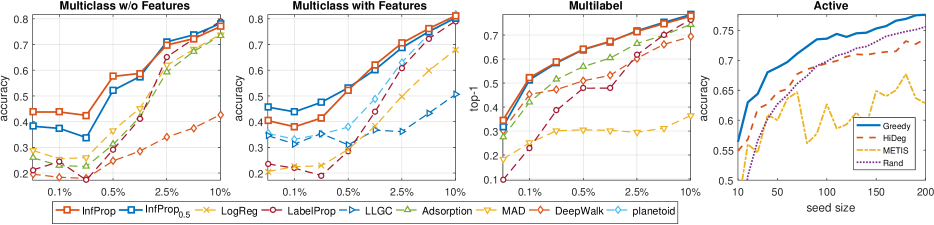
Figure 2: Results on the CoRA dataset for various learning settings.

4 Other Learning Settings

In this section we briefly describe how our method extends to other learning settings used in our experiments. For more details please see the supp. material.

Incorporating features and priors:

Many network-based datasets include additional node features or priors. Our method incorporates priors directly into the CTIC dynamics by penalizing incubation times. Denote by ${\bm{\rho}}_{v\ell}$ the prior for labeling $v$ with $\ell$, and let ${q}:[0,1]\rightarrow\mathbb{R}$ be a penalty function. If $u$ succeeds in infecting $v$ with $\ell$, the incubation time $\delta_{uv}$ is penalized by an additional ${q}({\bm{\rho}}_{v\ell})$. For a monotone decreasing ${q}$, high priors induce low penalties, and vice versa. Although penalties are deployed locally, they delay the propagation of the penalized label across the graph in a global manner.

Confidence and active learning:

Recall that $v$ remains uninfected with probability $f_{v0}$. Hence, ${\sigma}_{v}({S})=1-{f}_{v0}$ serves as a natural measure of confidence. We use this as a selection criteria for an active setting where the goal is to choose a seed set of size $k$. The objective we consider coincides with the well-studied notion of influence [26], which is monotone and submodular and admits to an efficient greedy approximation scheme. Our method thus offers a tractable alternative to existing active SSL methods [24, 18, 22].

5 Related Work

Methods for SSL are often based on assumptions regarding the structure of the unlabeled data. One such assumption is smoothness, which states that examples that are close are likely to have similar labels. In the classic Label Propagation algorithm [47], adjacent nodes in the graph are encouraged to agree on their labels via a quadratic penalty. Some variants add regularization terms [4], allow for label uncertainty [42], or include normalization and unanchored seeds [46].

The above methods are designed for graphs that approximate the data density via similarity in feature space, and are typically constructed from samples. Recent SSL methods are geared towards tasks where graphs are an additional part of the input. Motivated by deep embeddings [32], these methods embed the nodes of a graph into a low-dimensional vector space, which can then be used in various ways. When the data includes only the graph, the embeddings can be used as input for an off-the-shelf predictor [36]. When the data includes additional node features, the embedding can act as a regularizer for a standard loss over the labeled nodes [45, 28]. In contrast to classic methods, these methods propagate features rather than labels.

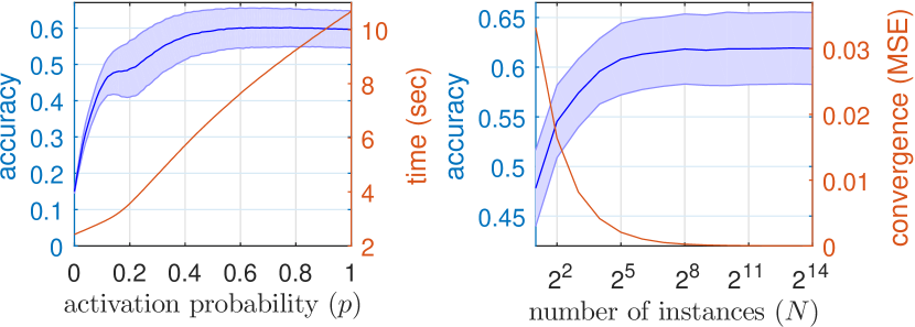
Figure 3: Activation tradeoff and convergence

An alternative method for utilizing graphs is to consider shortest paths as a measure of closeness. The authors of [1] show that Laplacians and shortest paths are special cases of “resistance distances”, and propose (but do not evaluate) a new regularizer. Other methods construct ad-hoc graphs whose shortest paths approximate density-based distances [35, 6]. A recent work [15] proposes a method for SSL in directed graphs based on distance diffusion. As they consider distances from unlabeled to labeled nodes, each instance is computationally intensive, and requires an approximation scheme. In contrast, we consider distances from labeled to unlabeled nodes, which can be computed efficiently. While for a specific setting (symmetric weights and a certain link function) both models overlap, in this paper we consider a more general setup.

Our method draws on the rich literature of infection models and diffusion processes over networks. These have been used for describing the propagation of information, innovation, behavioral norms, and others, and have been utilized in works in influence maximization [26], network inference [20], influence maximization [26] estimation [17, 16] and prediction [38], and personalized marketing [14].

	Multiclass (Accuracy / MSE)					Multilabel (AUC / Top-1)					[b]
	CoRA	DBLP	Flickr	IMDb	Industry	Amazon	CoRA	IMDb	PubMed	Wikipedia	YouTube
InfProp	0.59 / 0.56	0.73 / 0.42	0.79 / 0.38	0.56 / 0.49	0.21 / 0.91	0.79 / 0.56	0.91 / 0.67	0.75 / 0.36	0.90 / 0.77	0.93 / 0.70	0.84 / 0.38 [t]
InfProp0.5	0.58 / 0.64	0.74 / 0.46	0.78 / 0.38	0.55 / 0.49	0.21 / 0.90	0.79 / 0.57	0.90 / 0.67	0.76 / 0.36	0.88 / 0.77	0.94 / 0.71	0.84 / 0.40
ShortPaths	0.53 / 0.87	0.63 / 0.74	0.65 / 0.70	0.55 / 0.90	0.16 / 1.57	0.69 / 0.49	0.76 / 0.56	0.57 / 0.30	0.76 / 0.67	0.67 / 0.36	0.59 / 0.22
LabelProp	0.41 / 0.74	0.60 / 0.59	0.33 / 0.90	0.50 / 0.63	0.14 / 0.99	0.85 / 0.57	0.86 / 0.48	0.77 / 0.36	0.82 / 0.64	0.78 / 0.31	0.71 / 0.18
Adsorption	0.42 / 0.99	0.54 / 0.99	0.72 / 0.99	0.56 / 0.99	0.14 / 0.99	0.73 / 0.52	0.86 / 0.60	0.71 / 0.32	0.80 / 0.69	0.89 / 0.57	0.79 / 0.28
MAD	0.45 / 0.99	0.20 / 1.00	0.75 / 0.99	0.58 / 0.99	0.16 / 1.00	0.73 / 0.52	0.47 / 0.30	0.70 / 0.32	0.79 / 0.70	0.00 / 0.05	0.81 / 0.31
DeepWalk	0.29 / 0.86	0.77 / 0.62	0.49 / 0.73	0.50 / 0.56	0.17 / 0.92	0.60 / 0.13	0.80 / 0.53	0.61 / 0.32	0.57 / 0.42	0.94 / 0.88	0.60 / 0.24 [b]

Table 1: Results for experiments on data without features.

6 Experiments

We evaluated our method on various learning tasks over three benchmark dataset collections, which include networked data for multiclass learning with features [40] and without features [39], and multilabel learning [34]. The datasets include diverse networks such as social networks, citation and co-authorship graphs, product and item networks, and hyperlink graphs (see supplementary material for dataset summary statistics).

Our experimental setup follows the standard graph-based semi-supervised learning evaluation approach. Specifically, in each instance we draw a seed set of size $k$ uniformly at random, acquire its labels, and then use the graph and labeled seed set to generate labels for all nodes. We repeat this procedure for 10 random seed set selections and for various values of $k$ (where $k$ is set to be a fixed proportion of the number of nodes in the graph) and report average results.

We compared our method to current state-of-the-art baselines, which include spectral methods as well as deep embedding methods. For tasks which do not include features, these included LabelProp [47], Adsorption [4], MAD [42], and the feature-agnostic deep method DeepWalk [36]. For tasks which do include features, we compared to the prior-supporting spectral method LLGC [46], the recent feature-based deep method Planetoid [45], LabelProp as a graph-only baseline, logistic regression (LogReg) as a features-only baseline, and a baseline where labels are set by shortest paths in $G$ (ShortPaths). For the active setting (Fig. 2), we compared our approach (Greedy) to METIS [23], to choosing high-degree nodes (HiDeg), and to random seeds (Rand).

For our method (InfProp) we used exponential incubation times $\delta\sim\text{Exp}(\theta)$. As in many works (e.g., [26, 15]), we used $\theta_{uv}=1/d_{u}$ for all node pairs $(u,v)\in E$, where $d_{u}$ is the out-degree of $u$. We set the number of random instances to $N=1,000$. Fig. 3 (right) demonstrates accuracy and convergence as a function of $N$. We show results for two variants: InfProp, where we set activation probabilities to $p=1$ for all edges, and InfProp_0.5, where $p=0.5$. In addition to providing a confidence measure, InfProp_0.5 is much faster, while on average achieving 0.99% of the performance of InfProp. Fig. 3 (left) demonstrates the tradeoff in accuracy and runtime when varying $p$.

The methods we consider naturally output probabilistic “soft” labels as predictions. We therefore evaluate performance using both probabilistic (for multi-class) or order-based (for multi-label) performance measures, as well as performance measures for “hard” labels, which were generated by choosing the label with the highest value. Tables 1 and 2 include results for all datasets for $k=1\%$ of the data. Fig. 2 shows results for various values of $k$ on the CoRA dataset (which appears in all benchmarks). As shown, InfProp consistently performs well across all settings.

7 Conclusions

In this work we presented an SSL method where labels propagate over the graph using dynamic infection models. These models have a strong connection to short-path ensembles and to graph Laplacians, allow for efficient computation, and show empirical potential. Our work was motivated by the idea that different graph types may require different dynamics, which led us to consider alternatives to random walks and averaging dynamics. We used a competitive CTIC variant, but other infection models (and other dynamics in general) can be considered. The choice of dynamics can serve as a means for expressing prior knowledge and for encoding structure and dependencies.

The models we use have very few tunable parameters. Nonetheless, one can consider highly parametrized models. Such parameters can be used to control infection probabilities, be node or label specific, relate to features, and even adjust the dynamics themselves. The stochastic nature of the models and the nonlinearity of the dynamics makes learning these parameters a challenging task, which we leave for future work.

(Acc. / MSE)	CiteSeer	CoRA	PubMed
InfProp	0.47 / 0.72	0.62 / 0.59	0.74 / 0.46 [t]
InfProp0.5	0.48 / 0.74	0.60 / 0.57	0.72 / 0.41
ShortPaths	0.39 / 0.73	0.44 / 0.72	0.68 / 0.51
LogReg	0.44 / 0.78	0.37 / 0.81	0.45 / 0.65
LabelProp	0.39 / 0.77	0.38 / 0.78	0.40 / 0.67
LLGC	0.45 / 0.71	0.49 / 0.69	0.44 / 0.67
Planetoid	0.41 / 0.94	0.53 / 0.89	0.68 / 0.64 [b]

Table 2: Results on data with features.

Acknowledgments.

This work was supported by the Blavatnik Computer Science Research Fund and an ISF Centers of Excellence grant.

Supplamentary Material

1 Proof of Proposition 2 in Main Text

In this section we prove the correctness of our algorithm 2. The proof considers the more general CTIC infection dynamics and allows for node features or priors (via a penalty function).

In the infection dynamics presented in the paper, once a node’s label is set, it remains fixed. In contrast, during the course of the algorithm’s run, a node’s label may change with each distance update. It therefore remains to show that the algorithm outputs the desired labels. For basing our claim it will be easier to assume that instead of initially inserting all seed nodes into $Q$, we add a dummy root node ${r}$ to $V$, with edges of length $w_{{r}s}=0$ to all $s\in{S}$, and initialize $Q$ to include only ${r}$. It is easy to see that after extracting ${r}$ from $Q$, we return to our original algorithm.

Recall that the standard single-source Dijkstra algorithm offers three important guarantees: (1) the estimated distances of extracted nodes is correct (and remains unchanged), (2) nodes are extracted in increasing order of their true distance, and (3) the distance estimates always upper-bound the true distances.

Let $v\in{U}$ be a node that has just been extracted, and assume by induction that the labels of all previously extracted nodes (which include all seed nodes) are correct. The above guarantees tell us that the distance from ${r}$ to $v$ is correct, and all nodes on the shortest path from ${r}$ to $v$ have already been extracted. This is true even when a penalty is incurred, as it can only increase the distance estimate. As these nodes are assumed to be correctly labeled, $v$ inherits the correct label as well, as by construction its shortest path from ${r}$ goes through exactly one seed node. The correctness of the labels of the seed nodes gives the induction basis, which concludes the proof.

2 Extensions

In this section we give an in-depth description of several useful extensions of our method that were briefly discussed in the main text. These include applying out method to the Linear Threshold model, incorporating node features and priors into the infection dynamics, and a framework for using our method in an active SSL setting.

2.1 The Linear Threshold model

In this section we show how InfProp can be applied with the Linear Threshold (LT) dynamics, rather than the IC or CTIC dynamics discussed in the main text. This includes adapting the algorithm for computing expected labels to the LT model, as well as supporting node features and priors.

The input to the LT model is a weighted graph $G=(V,E,W)$ and an initial set of infected seed nodes ${S}$. We assume that weights are positive, and that for each $v\in V$, the sum of incoming weights $\sum_{v}W_{uv}$ is at most 1 (though it can be strictly less than 1). Before the process begins, each node $u$ is assigned a threshold $\eta_{u}$ sampled uniformly at random from the interval $[0,1]$. The dynamics then progress in discrete time steps, where at time $t$, a susceptible node $v$ becomes infected if the weighted sum of its infected neighbors exceeds its threshold. Denoting by $I_{u}(t)$ an indicator of whether $u$ is infected at time $t$, $v$ is infected at time $t$ if:

$$\sum_{u}W_{uv}I_{v}(t-1)\geq\eta_{u}$$ (14)

Note that the randomness in this model comes from the threshold $\eta$; given $\eta$, the dynamics are deterministic.

The authors of [26] show that the LT model can also be equivalently expressed via a graphical perspective using active edge sets. Here, however, edges are no longer sampled independently. Instead, for each node $v$, only at most one incoming edge will become active in each instance. Specifically, for each node $v$, each incoming edge $(u,v)\in E$ is selected to be the (only) edge with probability $p_{uv}=W_{uv}$, and with probability $W_{-u}=1-\sum_{v}W_{uv}$ no incoming edges are activated. Then, for a given instance, $v$ is infected if and only if there is an active path to $v$ from some seed node in ${S}$.

An interesting interpretation of the above is that the chosen active edge $(u,v)$ can be thought of as corresponding to the node $u$ whose infection triggered the infection of $v$ by crossing the threshold. Under this view, a label-dependent specification of the above model is one where $v$ inherits its label from its triggering neighbor $v$, which we refer to as his infector. This allows the model to be applied to the competitive setting which we consider. In terms of implementation, the only necessary modification to the algorithm is the way in which active edges are sampled.

The competitive LT model can also incorporate node priors using penalty terms. Specifically, the node-label prior ${\bm{\rho}}_{v\ell}$ will induce a multiplicative penalty ${q}_{v}(\ell)\in[0,1]$ on the original weights $W_{uv}$ when $u$ tries to infect $v$ with label $\ell$. Thus, given that $u$ has label $\ell$, the penalty reduces the probability that it will be the infector of $v$. To implement this, when $u$ is expanded, the edge $(u,v)$ is sampled to be active with the penalized probability, and all other incoming weights (including the complementing $W_{-u}$) are re-normalized.

2.2 Incorporating node features and priors

In addition to the graph, many network-based datasets include node or edge features. These can be used to generate node-specific class priors. In this section we describe a novel generalization of the competitive infection models introduced above which incorporates class priors into the dynamics. In this setting, our approach is to first train a probabilistic classifier (e.g., logistic regression) on the labeled seed set, and then use its predictions on the unlabeled nodes as a prior for our model.

Our method utilizes node priors by transforming them into penalties on incubation times. Consider a single instance of an infection process. Assume node $u$ has just been infected with label $\ell\in{\mathcal{Y}}$, and succeeded in its attempt to infect node $v$ with an incubation time of $\delta_{uv}$. If $\delta_{uv}$ is small, then it is very likely that $v$ will get infected with $\ell$ as well. On the other hand, if $\delta_{uv}$ is large, then other nodes might have a chance to infect $v$ with other labels. This motivates the idea of further penalizing the infection time of a node according to its prior. We do this by adding a label-dependent penalty ${q}_{v}(\ell)$ to $\delta_{uv}$, as a function of the prior ${\bm{\rho}}_{v\ell}$. We use the link function ${q}_{v}(\ell)=-\log({\bm{\rho}}_{v\ell})$, which maps low priors into large penalties, and high priors into low penalties, where ${\bm{\rho}}_{v\ell}=1$ entails no penalty. Hence, setting ${\bm{\rho}}_{v\ell}=1$ for all $v,\ell$ recovers the original model.

Note that while the priors are deployed locally, their effect is in fact global, as penalizing a node’s infection time delays the potential propagation of its acquired label throughout the graph. This increases the significance of nodes which are central to the infection process, and reduces the significance of those which play a small role in it, a property captured by our notion of confidence. The strength of the above formulation lies in its ability to introduce non-linear label dependencies to the actual infection dynamics. To see this, we can write the original predictions as:

$${f}=\mathbb{E}_{\delta\sim{D}}\left[{{\mathcal{A}}^{\delta}\mathcal{{S}}}\right]=\mathbb{E}_{\delta\sim{D}}\left[{{\mathcal{A}}^{\delta}}\right]\mathcal{{S}}$$ (15)

where ${\mathcal{A}}^{\delta}_{vs}={{\mathds{1}}_{\{{s={\alpha}(v)}\}}}$ indicates ancestors in $G^{\delta}$, and $\mathcal{{S}}_{s\ell}={{\mathds{1}}_{\{{y_{s}=\ell}\}}}$ indicates the seed nodes’ true labels. This shows that predictions are non-linear in the propagation of the seed nodes, but linear in the labels. In the prior-dependent model, the above no longer holds, as activation times are now label-dependent.

2.3 Confidence and Active Learning

Recall that a node $v$ has a probability $f_{v0}$ of not being infected by any label. This suggests a very natural measure of confidence in our prediction, namely:

$${\sigma}_{v}({S})=1-{f}_{v0}=\sum_{\ell=1}^{L}{f}_{v\ell},\qquad{\sigma}({S})=\sum_{v}{\sigma}_{v}(S)$$ (16)

The function ${\sigma}$ quantifies the confidence in the labeling. This is conceptually different from confidence in a label. Our model supports both concepts distinctly. The former is controlled by the activations $p$, as they determine reachability in the active graph and are agnostic to labels. The latter is controlled by $\theta$, as it affects the speed of propagation of the labels.

The notion of confidence allows us to apply our method to an active SSL setting. Instead of assuming the seed is given as input, in this setting we are allowed to choose the seed set, often under a cardinality constraint. The goal is then to choose the seed set which leads to a good labeling. Various graph-based notions have been suggested as objectives for active seed selection, such as those based on graph cuts [24], graph signals [18], and generalization error [22]. Such methods however either optimize an adversarial objective, or simply offer a heuristic solution. In contrast, using ${\sigma}$ as a seed-selection criterion offers an optimistic alternative, as summing over all classes makes it indifferent to the actual (latent) labels.

The confidence term ${\sigma}$ coincides with the well-studied notion of influence, defined as the expected number of nodes a seed will infect. In [26] it is shown that for various settings, influence is submodular, and therefore admits to a greedy $(1-1/\epsilon)$-approximation scheme. Any algorithm for maximizing influence efficiently (e.g., [16, 21]), can therefore be adopted for out setting.

3 Non-Homogeneous Laplacian

Here we prove that:

$${\mathcal{L}}({S})_{\vphantom{}}{f}={\bm{b}}({S})$$

where:

$${\bm{b}}_{u\ell}({S})=\sum_{v}b_{vu\ell}^{({S})},\qquad b_{vu\ell}^{({S})}=\text{cov}\left[{{T}_{vu}({S}),Y_{u\ell}}\right]$$

For clarity we drop the notational dependence on ${S}$. We begin by expanding ${f}_{u\ell}$ using $Y$ and $T$:

$${f}_{u\ell} =\mathbb{E}\left[{Y_{u\ell}}\right]=\mathbb{E}\left[{T_{u\cdotp}Y_{\cdotp\ell}}\right]$$

$$=\mathbb{E}\left[{\sum_{v}T_{uv}Y_{v\ell}}\right]$$

$$=\sum_{v}\mathbb{E}\left[{T_{uv}Y_{v\ell}}\right]$$

$$=\sum_{v}\left(\mathbb{E}\left[{T_{uv}}\right]\mathbb{E}\left[{Y_{v\ell}}\right]+\text{cov}\left[{T_{uv}Y_{v\ell}}\right]\right)$$

$$=\sum_{v}\left({\bm{{T}}}_{uv}{f}_{v\ell}+{b}_{uv\ell}\right)$$

where the final step is true for the product of general random variables. Rewriting in matrix form gives: ${f}={\bm{{T}}}{f}+{\bm{b}}$. Rearranging we get: $(I-{\bm{{T}}}){f}={\mathcal{L}}{f}={\bm{b}}$, as required.

The objective function can then be expressed as:

$$\|{\mathcal{L}}f^{\prime}-{\bm{b}}\|_{2}^{2} =\sum_{u}\sum_{\ell}\left({\mathcal{L}}_{u\cdotp}{f}_{\cdotp\ell}-{\bm{b}}_{u\ell}\right)^{2}$$

$$=\sum_{u}\sum_{\ell}\left(\sum_{v}{\mathcal{L}}_{uv}{f}_{v\ell}-{b}_{uv\ell}\right)^{2}$$

$$=\sum_{u}\sum_{\ell}\left(\sum_{v}({{\mathds{1}}_{\{{u=v}\}}}-{\bm{{T}}}_{uv}){f}_{v\ell}-{b}_{uv\ell}\right)^{2}$$

$$=\sum_{u}\sum_{\ell}\left(f_{u\ell}-\sum_{v}(w_{uv}{f}_{v\ell}+{b}_{uv\ell})\right)^{2}$$

where $w_{uv}={\bm{{T}}}_{uv}$.

4 Details for the Illustrative Synthetic Experiment

Our general hypothesis in this work is that infection dynamics are a good candidate for propagating label information over real networks. To illustrate this, we designed a synthetic experimental setup in which our goal was to capture the structure of real world networks. One well-known property of such networks is that they often have a community-like structure, with many intra-community edges, but few inter-community edges. In many cases, only a few specific nodes within a community are also connected to other communities. Hence, we randomly created small networks with the above properties.

Specifically, each network was set to have 3 (possibly overlapping) communities, each with 64 nodes. Nodes were randomly assigned into one community, and in each community, 8 nodes were randomly assigned to an additional community. To account for some noise, all other edges were added with probability 0.05. The seed set included one randomly chosen node from each community, giving $|{S}|=3$. The figure in the main text displays a random instance of the above setting, providing both the instance specific accuracies, as well as the average accuracy over 1,000 random instances.

Recall that InfProp can be interpreted both as the expected result of a dynamic infection process and as a stochastic ensemble of shortest paths. We therefore compared our method to two baselines. To compare the dynamics, we used Label Propagation (LabelProp) which is based on the more standard random-walk dynamics. As we argue in the text, these dynamics are prone to getting stuck in dense clusters. As can be seen, while InfProp provides almost exact predictions, the predictive values of LabelProp are almost uniform and hence extremely error-prone. This demonstrates the inability of label information to propagate efficiently over the network.

To demonstrate the power of using a stochastic ensemble of paths, we compared to simply setting labels according to the deterministic shortest paths given by the original graph. While correctly classifying most labels, shortest paths can be very sensitive to cross-community or noisy edges. In contrast, InfProp mitigates this noise by considering a distribution over shortest-paths.

5 Datasets

We evaluated our method on various learning tasks over three collections of benchmark datasets, which include network based datasets for multi-class learning with features[40], multi-class learning without features[39], and multi-label learning[34]. The following table provides some statistics.

	Dataset	Nodes	Edges	Classes	Features	Avg. $|y|$
Multiclass	CoRA	2,708	5,278	7	-	1 [t]
	DBLP	5,329	21,880	6	-	1
	Flickr	7,971	478,980	7	-	1
	IMDb	2,411	12,255	22	-	1
	Industry	2,189	11,666	12	-	1 [b]
Features	CiteSeer	3,132	4,713	6	3,703	1 [t]
	CoRA	2,708	5,278	7	1,433	1
	PubMed	19,717	44,324	3	500	1 [b]
Multilabel	Amazon	83,742	190,097	30	-	1.546 [t]
	CoRA	24,519	92,207	10	-	1.004
	IMDb	19,359	362,079	21	-	2.300
	PubMed	19,717	44,324	3	-	1
	Wikipedia	35,633	49,538	16	-	1.312
	YouTube	22,693	96,361	47	-	1.707 [b]

References

- [1] Alamgir, M., and Luxburg, U. V. Phase transition in the family of p-resistances. In Advances in Neural Information Processing Systems (2011), pp. 379–387.
- [2] Aleliunas, R., Karp, R. M., Lipton, R. J., Lovasz, L., and Rackoff, C. Random walks, universal traversal sequences, and the complexity of maze problems. In Foundations of Computer Science, 1979., 20th Annual Symposium on (1979), IEEE, pp. 218–223.
- [3] Altun, Y., McAllester, D., and Belkin, M. Maximum margin semi-supervised learning for structured variables. Advances in neural information processing systems 18 (2006), 33.
- [4] Baluja, S., Seth, R., Sivakumar, D., Jing, Y., Yagnik, J., Kumar, S., Ravichandran, D., and Aly, M. Video suggestion and discovery for youtube: taking random walks through the view graph. In Proceedings of the 17th international conference on World Wide Web (2008), ACM, pp. 895–904.
- [5] Belkin, M., and Niyogi, P. Semi-supervised learning on Riemannian manifolds. Machine Learning 56, 1 (2004), 209–239.
- [6] Bijral, A. S., Ratliff, N., and Srebro, N. Semi-supervised learning with density based distances. In Proceedings of the Twenty-Seventh Conference on Uncertainty in Artificial Intelligence (2011), UAI’11, pp. 43–50.
- [7] Blum, A., and Chawla, S. Learning from labeled and unlabeled data using graph mincuts. Proc. 18th International Conf. on Machine Learning (2001).
- [8] Borodin, A., Filmus, Y., and Oren, J. Threshold models for competitive influence in social networks. In WINE (2010), vol. 6484, Springer, pp. 539–550.
- [9] Broder, A. Z., Karlin, A. R., Raghavan, P., and Upfal, E. Trading space for time in undirected s-t connectivity. SIAM Journal on Computing 23, 2 (1994), 324–334.
- [10] Budak, C., Agrawal, D., and El Abbadi, A. Limiting the spread of misinformation in social networks. In Proceedings of the 20th international conference on World wide web (2011), ACM, pp. 665–674.
- [11] Chapelle, O., Schölkopf, B., Zien, A., et al. Semi-supervised learning. MIT press Cambridge, 2006.
- [12] Chen, W., Collins, A., Cummings, R., Ke, T., Liu, Z., Rincon, D., Sun, X., Wang, Y., Wei, W., and Yuan, Y. Influence maximization in social networks when negative opinions may emerge and propagate. In Proceedings of the 2011 SIAM International Conference on Data Mining (2011), SIAM, pp. 379–390.
- [13] Chen, W., Lakshmanan, L. V., and Castillo, C. Information and influence propagation in social networks. Synthesis Lectures on Data Management 5, 4 (2013), 1–177.
- [14] Chen, W., Wang, C., and Wang, Y. Scalable influence maximization for prevalent viral marketing in large-scale social networks. In Proceedings of the 16th ACM SIGKDD international conference on Knowledge discovery and data mining (2010), ACM, pp. 1029–1038.
- [15] Cohen, E. Semi-supervised learning on graphs through reach and distance diffusion. arXiv preprint arXiv:1603.09064 (2016).
- [16] Cohen, E., Delling, D., Pajor, T., and Werneck, R. F. Sketch-based influence maximization and computation: Scaling up with guarantees. In Proceedings of the 23rd ACM International Conference on Conference on Information and Knowledge Management (2014), ACM, pp. 629–638.
- [17] Du, N., Song, L., Rodriguez, M. G., and Zha, H. Scalable influence estimation in continuous-time diffusion networks. In Advances in neural information processing systems (2013), pp. 3147–3155.
- [18] Gadde, A., Anis, A., and Ortega, A. Active semi-supervised learning using sampling theory for graph signals. In Proceedings of the 20th ACM SIGKDD international conference on Knowledge discovery and data mining (2014), ACM, pp. 492–501.
- [19] Goldenberg, J., Libai, B., and Muller, E. Talk of the network: A complex systems look at the underlying process of word-of-mouth. Marketing letters 12, 3 (2001), 211–223.
- [20] Gomez Rodriguez, M., Leskovec, J., and Krause, A. Inferring networks of diffusion and influence. In Proceedings of the 16th ACM SIGKDD International Conference on Knowledge Discovery and Data Mining (2010), KDD ’10, pp. 1019–1028.
- [21] Gomez-Rodriguez, M., Song, L., Du, N., Zha, H., and Schölkopf, B. Influence estimation and maximization in continuous-time diffusion networks. ACM Trans. Inf. Syst. 34, 2 (Feb. 2016), 9:1–9:33.
- [22] Gu, Q., and Han, J. Towards active learning on graphs: An error bound minimization approach. In Data Mining (ICDM), 2012 IEEE 12th International Conference on (2012), IEEE, pp. 882–887.
- [23] Guillory, A., and Bilmes, J. A. Label selection on graphs. In Advances in Neural Information Processing Systems (2009), pp. 691–699.
- [24] Guillory, A., and Bilmes, J. A. Active semi-supervised learning using submodular functions. In UAI 2011, Proceedings of the Twenty-Seventh Conference on Uncertainty in Artificial Intelligence (2011), pp. 274–282.
- [25] He, X., Song, G., Chen, W., and Jiang, Q. Influence blocking maximization in social networks under the competitive linear threshold model. In Proceedings of the 2012 SIAM International Conference on Data Mining (2012), SIAM, pp. 463–474.
- [26] Kempe, D., Kleinberg, J., and Tardos, É. Maximizing the spread of influence through a social network. In Proceedings of the ninth ACM SIGKDD international conference on Knowledge discovery and data mining (2003), ACM, pp. 137–146.
- [27] Kermack, W. O., and McKendrick, A. G. A contribution to the mathematical theory of epidemics. Proceedings of the Royal Society of London A: Mathematical, Physical and Engineering Sciences 115, 772 (1927), 700–721.
- [28] Kipf, T. N., and Welling, M. Semi-supervised classification with graph convolutional networks. arXiv preprint arXiv:1609.02907 (2016).
- [29] Lin, F., and Cohen, W. W. The multirank bootstrap algorithm: Self-supervised political blog classification and ranking using semi-supervised link classification. In Proceedings of the Second International Conference on Weblogs and Social Media, ICWSM 2008, Seattle, Washington, USA, March 30 - April 2, 2008 (2008).
- [30] Lofgren, P., Banerjee, S., Goel, A., and Comandur, S. FAST-PPR: scaling personalized pagerank estimation for large graphs. In The 20th ACM SIGKDD International Conference on Knowledge Discovery and Data Mining, KDD ’14, New York, NY, USA - August 24 - 27, 2014 (2014), pp. 1436–1445.
- [31] Martín, P. J., Torres, R., and Gavilanes, A. Cuda solutions for the sssp problem. In International Conference on Computational Science (2009), Springer, pp. 904–913.
- [32] Mikolov, T., Sutskever, I., Chen, K., Corrado, G. S., and Dean, J. Distributed representations of words and phrases and their compositionality. In Advances in neural information processing systems (2013), pp. 3111–3119.
- [33] Nadler, B., Srebro, N., and Zhou, X. Semi-supervised learning with the graph laplacian: The limit of infinite unlabelled data. Advances in neural information processing systems 21 (2009).
- [34] Nandanwar, S., and Murty, M. N. Structural neighborhood based classification of nodes in a network. In Proceedings of the 22Nd ACM SIGKDD International Conference on Knowledge Discovery and Data Mining (2016), KDD ’16, pp. 1085–1094.
- [35] Orlitsky, A., et al. Estimating and computing density based distance metrics. In Proceedings of the 22nd international conference on Machine learning (2005), ACM, pp. 760–767.
- [36] Perozzi, B., Al-Rfou, R., and Skiena, S. Deepwalk: Online learning of social representations. In Proceedings of the 20th ACM SIGKDD international conference on Knowledge discovery and data mining (2014), ACM, pp. 701–710.
- [37] Rifai, S., Dauphin, Y., Vincent, P., Bengio, Y., and Muller, X. The manifold tangent classifier. In NIPS (2011), vol. 271, p. 523.
- [38] Rosenfeld, N., Nitzan, M., and Globerson, A. Discriminative learning of infection models. In Proceedings of the Ninth ACM International Conference on Web Search and Data Mining (2016), WSDM ’16, pp. 563–572.
- [39] Saha, T., Rangwala, H., and Domeniconi, C. Flip: active learning for relational network classification. In Joint European Conference on Machine Learning and Knowledge Discovery in Databases (2014), Springer, pp. 1–18.
- [40] Sen, P., Namata, G. M., Bilgic, M., Getoor, L., Gallagher, B., and Eliassi-Rad, T. Collective classification in network data. AI Magazine 29, 3 (2008), 93–106.
- [41] Sindhwani, V., Niyogi, P., and Belkin, M. Beyond the point cloud: from transductive to semi-supervised learning. In Proceedings of the 22nd international conference on Machine learning (2005), ACM, pp. 824–831.
- [42] Talukdar, P. P., and Crammer, K. New regularized algorithms for transductive learning. In Joint European Conference on Machine Learning and Knowledge Discovery in Databases (2009), Springer, pp. 442–457.
- [43] Vishnoi, N. K., et al. Lx= b. Foundations and Trends in Theoretical Computer Science 8, 1–2 (2013), 1–141.
- [44] von Luxburg, U., Radl, A., and Hein, M. Getting lost in space: Large sample analysis of the resistance distance. In Advances in Neural Information Processing Systems (2010), pp. 2622–2630.
- [45] Yang, Z., Cohen, W. W., and Salakhutdinov, R. Revisiting semi-supervised learning with graph embeddings. In Proceedings of the 33rd International Conference on International Conference on Machine Learning (2016), ICML’16, pp. 40–48.
- [46] Zhou, D., Bousquet, O., Lal, T. N., Weston, J., and Schölkopf, B. Learning with local and global consistency. In NIPS (2003), vol. 16, pp. 321–328.
- [47] Zhu, X., Ghahramani, Z., Lafferty, J., et al. Semi-supervised learning using gaussian fields and harmonic functions. In ICML (2003), vol. 3, pp. 912–919.