Closed Superstring Field Theory and its Applications

^aEcole normale superieure, 24 rue Lhomond, F-75230 Paris cedex 05, France

^bHarish-Chandra Research Institute, HBNI, Chhatnag Road, Jhusi, Allahabad 211019, India

^cInternational Centre for Theoretical Sciences, Hesarghatta, Bengaluru 560089, India.

E-mail: corinne.delacroix,harold.erbin@lpt.ens.fr, sitenderpratap,sen,mritunjayverma@hri.res.in

Abstract

We review recent developments in the construction of heterotic and type II string field theories and their various applications. These include systematic procedures for determining the shifts in the vacuum expectation values of fields under quantum corrections, computing renormalized masses and S-matrix of the theory around the shifted vacuum and a proof of unitarity of the S-matrix. The S-matrix computed this way is free from all divergences when there are more than 4 non-compact space-time dimensions, but suffers from the usual infrared divergences when the number of non-compact space-time dimensions is 4 or less.

1 Introduction and Motivation

In string theory the observables are S-matrix elements – also called amplitudes. These are the observables in field theories as well. However, the prescription for computing the S-matrix in string theory is apparently different from that in quantum field theories. A $g$-loop, $N$-point amplitude is given by an expression of the form:

$$\int dm_{1}\ldots dm_{6g-6+2N}\,F(m_{1},m_{2},\ldots,m_{6g-6+2N})$$ (1.1)

where $m_{i}$ are the parameters labelling the moduli space of two dimensional Riemann surfaces of genus $g$ and $n$ marked points – also known as punctures. $F(\{m_{i}\})$ denotes a correlation function of a two dimensional conformal field theory on the Riemann surface, with vertex operators for external states inserted at the punctures and additional insertions of ghost fields and picture changing operators (PCO)[1] that do not depend on the external states. In particular, at any given loop order there is only one term, while in a quantum field theory for a similar amplitude, there will be many terms representing contributions from different Feynman diagrams. Given these differences, we may wonder if there is any similarity between string theory amplitudes and ordinary quantum field theory amplitudes.

The closest comparison between string theory amplitudes and the amplitudes in an ordinary quantum field theory can be made in Schwinger parameter representation of the latter, in which we replace the denominator factors of each propagator by an integral:

$$(k^{2}+m^{2})^{-1}=\int_{0}^{\infty}ds\,e^{-s(k^{2}+m^{2})}\,.$$ (1.2)

With this replacement, the integration over loop momenta takes the form of gaussian integrals, possibly multiplied by a polynomial in momenta arising from vertices and propagators, and the integrals can be easily performed. The result takes the form

$$\int ds_{1}\ldots ds_{n}\,f(s_{1},\ldots,s_{n})$$ (1.3)

where $s_{1},\ldots,s_{n}$ are the Schwinger parameters for the $n$ propagators and $f(\{s_{i}\})$ is some function of these parameters that we obtain after integration over momenta. At a very crude level, in string theory the parameters $\{m_{i}\}$ labelling the moduli space of Riemann surfaces play the role of the Schwinger parameters $\{s_{i}\}$, and the integrand $F$ appearing in (1.1) plays the role of the function $f$ appearing in (1.3).

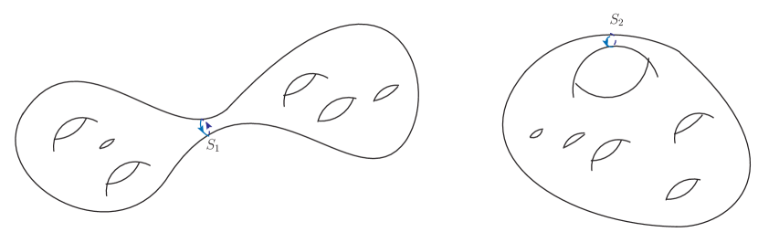
Figure 1: The left figure shows a Riemann surface near a separating type degeneration and the right figure shows a Riemann surface near a non-separating type degeneration. The degeneration happens when $S_{1}$ and $S_{2}$ shrink to a point.

In quantum field theories we typically have both ultraviolet (UV) and infrared (IR) divergences. The UV divergences arise from regions of integration where one or more loop momenta become large, while IR divergences arise from regions of integration where one or more propagators have vanishing denominator. In the Schwinger parameter representation where all loop momenta integrations have already been performed, the UV divergences arise from the region where one or more Schwinger parameter vanishes, and the IR divergences arise from the region where one or more Schwinger parameter becomes infinite.

Figure 2: The left figure shows the Feynman diagrams in field theory analogous to a separating type degeneration and the right figure shows the Feynman diagrams in field theory analogous to a non-separating type degeneration. The blobs represent arbitrary Feynman diagrams, and the thick lines represent propagators whose Schwinger parameters go to infinity in the degeneration limit.

The string theory amplitudes (1.1) also suffer from divergences. These divergences come from near the boundary of the moduli space where the Riemann surface degenerates. As shown in Fig. 1, the degeneration can be of two types – separating type degeneration in which the Riemann surface breaks apart into two parts and non-separating type degeneration in which the Riemann surface breaks into a lower genus surface with two extra punctures. Examination of the integrand $F$ in (1.1) in this limit shows that the integrand behaves in a way similar to the integrand $f$ in the field theory expression in the limit where the Schwinger parameter of a propagator approaches infinity. The corresponding field theory Feynman diagrams have been shown in Fig. 2, where the thick lines represent the propagators with large Schwinger parameters.

Figure 3: A tree level diagram that encounters type 1 divergence when the total energy flowing along the horizontal line exceeds the threshold for producing an on-shell single particle intermediate state.

Since, in field theory, divergences for large Schwinger parameters represent IR divergences, we conclude that the divergences in string theory, arising from degenerate Riemann surfaces, are IR divergences. Therefore, in order to deal with IR divergences in string theory, it will be instructive to see what kind of divergences arise in quantum field theories in the large Schwinger parameter regime and how they are resolved. They can be classified into two categories:

1. For $k^{2}+m^{2}<0$, the left hand side of (1.2) is finite but the right hand side diverges. As shown in Fig. 3, such a divergence can arise even at the tree level. In a quantum field theory this is easily dealt with by working directly with the left hand side, i.e. in the momentum space representation of the Feynman amplitudes. This option does not exist in the conventional formulation of superstring perturbation theory. The second option, which can be generalized to string theory[2, 3], is to treat the Schwinger parameters as complex variable and treat the integration over these variables as contour integrals with the upper limit taken to be $i\infty$ instead of $\infty$. A closely related third approach is to write the amplitude with the external momenta in the region where such divergences are absent and then define the amplitude in other regions via analytic continuation. Examples of such divergences in string theory include those arising from two or more vertex operators in the world-sheet coming close, e.g. the apparent divergences in the integral representation of Virasoro-Shapiro amplitude in certain kinematic regime.

2. For $(k^{2}+m^{2})=0$, both the left hand side and the right hand side of (1.2) diverge. These are genuine divergences in quantum field theories in which some internal propagator is forced to be on-shell. Examples of such diagrams are mass renormalization diagrams and massless tadpole diagrams as shown in Fig. 4. In quantum field theory, these divergences have standard remedies. For example, the presence of tadpole diagrams in a quantum field theory indicates that the tree level vacuum is modified by quantum corrections. We deal with these divergences by first constructing the one particle irreducible (1PI) effective action, finding its extremum and then expanding the action around the new extremum to reorganize the perturbation expansion. Similarly, the divergences associated with the mass renormalization diagrams are removed by first finding the solution to the linearized equations of motion of 1PI effective action around the extremum to determine the renormalized mass of the particle, and then computing the S-matrix using the LSZ prescription. In this approach, diagrams of the type shown in Fig. 4 never appear, but we have to compensate for it in other ways that involve correcting the interaction terms and/or masses. However, in conventional superstring perturbation theory, there is no well defined procedure for removing these divergences, essentially due to the fact that at each loop there is a single term, and there is no fully systematic procedure for removing some parts of this contribution and compensating for this in other ways[4, 5, 6, 7, 8, 9, 10, 11, 12, 13, 14, 15, 16, 17]. Even when these divergences are absent, the final results for S-matrix computed using standard rules have apparent ambiguities[18, 19, 20] which need to be absorbed into redefinitions of moduli fields and / or wave-function renormalization factors[21, 20].

One of our goals in this review will be to describe how superstring field theory can be used to remove these divergences. Along the way, we shall also see various other applications of superstring field theory. We shall mostly follow the approach described in [22, 23, 24, 25, 26, 27, 28, 29].

Figure 4: The figure on the left shows a divergence associated with massless tadpoles. The thick line is forced to carry zero momentum due to momentum conservation. Therefore if it represents a massless particle, the propagator diverges. The diagram on the right shows divergences associated with mass renormalization. Requiring the external line to be on-shell also puts the internal line marked by the thick line on-shell, causing a divergence.

What is superstring field theory? By requirement, superstring field theory is a quantum field theory whose amplitudes, computed with Feynman diagrams, have the following properties:

1. They agree with standard superstring amplitudes when the latter are finite.

2. They agree with analytic continuation of standard superstring amplitudes when the latter are finite.

3. They formally agree with standard superstring amplitudes when the latter have genuine divergences. However, in superstring field theory we should be able to deal with these divergences using standard field theory techniques like mass renormalization and shift of vacuum.

The question is: Does such a theory exist? For open and closed bosonic string theory such a theory has been known to exist for a long time[30, 31, 32, 33, 34, 35]. There have been various approaches to constructing tree level open superstring and closed heterotic string field theories[36, 37, 38, 39, 40, 41, 42, 43, 44, 45, 46, 47, 48, 49, 50, 51, 52, 53, 54, 55, 56, 57, 58, 59, 60, 61, 62, 63, 64, 65]. Some of these have been discussed briefly in section 10. However, there is an apparent no go theorem ruling out the existence of such theories for type IIB superstrings. It goes as follows. If we can construct an action for type IIB superstring theory then by taking its low energy limit we should get an action for type IIB supergravity. However, it is known that it is impossible to construct such an action due to the existence of the four form gauge field with self-dual field strength in this theory. Therefore, it follows that we should not be able to construct an action for type IIB superstring field theory. While this does not rule out the possibility of having type IIA or heterotic string field theories, it shows that there cannot be a generic formalism covering all superstring theories.

It turns out that there is a way to circumvent this no-go theorem as follows[23, 25]. It is possible to construct actions for heterotic and type II string field theories, but each of these theories contains an additional set of “ghost”-like particles which are free. These additional particles are unobservable since they do not scatter. Therefore, their existence can be ignored for all practical purposes except that the fields corresponding to these particles are necessary to construct the kinetic term of the action. Using this formalism one can now construct heterotic and type II superstring field theories – collectively called superstring field theory – not only at the tree level but also at the full quantum level[22, 23, 25]. In the following sections, we shall describe the structure of these theories in detail. This construction closely follows the structure of the closed bosonic string field theory[34], with few additional twists.

Once a superstring field theory is formulated, the divergences associated with massless tadpoles and mass renormalizations, illustrated in Fig. 4, can be dealt with using standard techniques of quantum field theory[22, 23, 24]. This leads to an unambiguous, divergence free definition of S-matrix elements when the number of non-compact space-time dimensions is $\geq 5$. Furthermore, this S-matrix can be shown to be unitary[26, 27, 28]. When the number of non-compact space-time dimensions is four or less, there is another kind of infrared divergence that comes from loops involving massless particles. These are reflections of the fact that we cannot distinguish between a final state with no massless particles from a final state with massless particles if the energy carried by the massless particles is sufficiently low or if the opening angle between two or more massless particles in the final state is sufficiently low. In quantum field theory one can show that these infrared divergences go away if in the cross section we sum over final state soft particles and collinear massless particles– i.e. not calculate the cross section for a fixed final state but a fixed final state accompanied by arbitrary number of soft particles carrying total energy below some fixed value and/or almost collinear massless particles with opening angle below some fixed value – and average over initial state soft and collinear particles[66, 67, 68, 69]. The analogue of this result for superstring field theory has not yet been established, but we do not expect any unsurmountable difficulty in establishing this.

The rest of this review is organized as follows. In section 2 we describe the construction of off-shell amplitudes of superstring field theory, without worrying whether they come from an underlying superstring field theory. In section 3 we describe the condition under which the off-shell amplitudes arise from the Feynman diagram of a superstring field theory, and explicitly construct the action of the gauge fixed superstring field theory. In section 4 we describe the quantum master action, whose Batalin-Vilkovisky (BV) quantization gives the gauge fixed action of section 3. In section 5 we derive the Ward identities for the off-shell amputated Green’s functions of this superstring field theory. At this stage this still remains a formal derivation, since this Green’s function is divergent in the presence of massless tadpoles. We also describe the construction of the effective action obtained by integrating out a subset of the fields of the theory and also construct the gauge invariant 1PI effective action. These are free from all divergences. In section 6 we describe how using the 1PI action constructed in section 5, we can find the vacuum solution and expand the action around it to find the renormalized masses and the unbroken (super-)symmetries. We also construct the Siegel gauge propagator and the interaction terms of the action expanded around the vacuum solution so that the Feynman diagrams computed using these vertices and propagators are free from tadpole and mass renormalization divergences. In section 7 we derive the Ward identities of the divergence free amplitudes computed from this new action. In section 8 we formulate the Feynman rules of string field theory in momentum space as in conventional quantum field theories and show that the rules for integration over the loop energies need to be modified in order to get UV finite results. In section 9 we make use of the momentum space Feynman rules of section 8 to prove unitarity of the S-matrix of superstring field theory. In section 10 we briefly discuss some of the other approaches used in the construction of superstring field theories. Appendix A contains a summary of notations and conventions while the rest of the appendices provide various supplementary material containing some details that were left out in the main text and also some simple examples illustrating some of the points discussed in the text.

We end this section by describing some of the notations and conventions we shall use, as well as the scope and limitations of this review. As already mentioned in footnote 1, superstring will refer to either of the heterotic string theories or either of the type II string theories, possibly compactified on a manifold with NS (NSNS for type II) background. The latter restriction is due to the fact that conformal invariance of the world-sheet theory will play an important role in this construction and at present the world-sheet description of string theory in an RR background has not been fully understood. If the pure spinor approach[70, 71] can be made into a fully workable formalism that works to all orders in superstring perturbation theory, then the present approach may be extendable to RR background as well. We shall also keep away from type I string theory, but we expect that this formalism can be generalized to type I theories with minor changes. We shall use the formalism of picture changing operators (PCO) to define amplitudes in superstring theory. For on-shell amplitudes there is an alternative formalism based on integration over supermoduli space[72, 73, 74, 75, 76, 77, 20, 78, 79, 80, 81, 82, 83, 84, 85, 86]. So far, off-shell generalization of these amplitudes have not been written down except for partial construction of tree level open string field theory[87], but in future it may be possible to reformulate the whole analysis described here by expressing the off-shell amplitudes as integrals over supermoduli spaces.

While our approach will be based on a manifestly Lorentz covariant formulation of superstring field theory, there is an alternative approach, known as light-cone string field theory, that only manifestly preserves the $SO(d-1)$ subgroup of the $SO(d,1)$ Lorentz group. This approach has been successful for bosonic string theory[88, 89], but there are various contact term ambiguities when we consider superstring field theory which have not been completely resolved[90, 91, 92, 93, 94, 95, 96].

We shall set $\alpha^{\prime}=1$ and define the mass² level of a state carrying momentum $k$ to be the eigenvalue of the operator $2(L_{0}+\bar{L}_{0})-k^{2}$ where $L_{0}$ and $\bar{L}_{0}$ denote zero modes of the total Virasoro generators. Physically this gives the squared mass of the state at tree level if it corresponds to a physical state of string theory.

Finally we would like to remark that in this review our focus will be on the application of closed superstring field theory in making superstring perturbation theory well defined. For instance, as mentioned earlier, one of the applications of this formalism is in proving the unitarity of the theory in the situations when the perturbation theory can be trusted. Treating the situation beyond perturbation theory, e.g., proving unitarity in the presence of black holes, can’t be dealt in this approach. The close cousin of closed superstring theory, namely open string field theory, has been used to construct non-trivial classical solutions, going beyond what can be achieved in perturbation theory[97]. Similar applications of closed string field theory remains beyond reach to this day despite some tantalizing numerical results in closed bosonic string field theory[98].

2 Off-shell amplitudes in superstring theory

In this section we shall follow [99, 100] to describe construction of off-shell amplitudes in superstring theory without demanding that they arise from an underlying field theory. For definiteness we shall restrict most of the discussions to heterotic string theory, and later comment on the additional ingredients necessary for extending the results to type II string theory.

2.1 World-sheet theory

The world-sheet theory for any heterotic string compactification at string tree level contains a matter superconformal field theory with central charge (26,15) and a ghost system of total central charge $(-26,-15)$. For the matter sector, we denote by $T_{m}$ and $T_{F}$ the right-moving stress tensor and its superpartner and by $\bar{T}_{m}$ the left-moving stress tensor. They satisfy the operator product expansion

$$T_{m}(z)T_{m}(w)={15\over 2}{1\over(z-w)^{4}}+\cdots,$$ (2.1)

$$T_{F}(z)T_{F}(w)={5\over 2}{1\over(z-w)^{3}}+{1\over 2}{1\over z-w}T_{m}(w)+\cdots,$$

$$T_{m}(z)T_{F}(w)={3\over 2}{1\over(z-w)^{2}}T_{F}(w)+{1\over z-w}\partial T_{F}(w)+\cdots,$$

$$\bar{T}_{m}(\bar{z})\bar{T}_{m}(\bar{w})={26\over 2}{1\over(\bar{z}-\bar{w})^{4}}+\cdots,$$

where $\cdots$ denote less singular terms.

The ghost system consists of anti-commuting $b$, $c$, $\bar{b}$, $\bar{c}$ ghosts and the commuting $\beta,\gamma$ ghosts. The $(\beta,\gamma)$ system can be bosonized as[1]

$$\gamma=\eta\,e^{\phi},\quad\beta=\partial\xi\,e^{-\phi},\quad\delta(\gamma)=e^{-\phi},\quad\delta(\beta)=e^{\phi}\,,$$ (2.2)

where $\xi,\eta$ are fermions of conformal weights $(0,0)$ and $(0,1)$ respectively and $\phi$ is a scalar with background charge. The operator products of these fields take the form

$$c(z)b(w)=(z-w)^{-1}+\cdots,$$ (2.3)

$$\bar{c}(\bar{z})\bar{b}(\bar{w})=(\bar{z}-\bar{w})^{-1}+\cdots,$$

$$\xi(z)\eta(w)=(z-w)^{-1}+\cdots,$$

$$e^{q_{1}\phi(z)}e^{q_{2}\phi(w)}=(z-w)^{-q_{1}q_{2}}e^{(q_{1}+q_{2})\phi(w)}+\cdots\,,$$

$$\partial\phi(z)\,\partial\phi(w)=-{1\over(z-w)^{2}}+\cdots\,,$$

where $\cdots$ denote less singular terms. The stress tensors of the ghost fields are given by

$$T_{b,c}=-2\,b\,\partial\,c+c\,\partial\,b,\quad\bar{T}_{\bar{b},\bar{c}}=-2\,\bar{b}\,\bar{\partial}\,\bar{c}+\bar{c}\,\bar{\partial}\,\bar{b},$$ (2.4)

$$T_{\beta,\gamma}(z)={3\over 2}\beta\partial\gamma+{1\over 2}\gamma\partial\beta=T_{\phi}+T_{\eta,\xi}\,,$$ (2.5)

where

$$T_{\eta,\xi}=-\eta\partial\xi\,,$$ (2.6)

and

$$T_{\phi}=-{1\over 2}\partial\phi\partial\phi-\partial^{2}\phi\,.$$ (2.7)

With this the total $\phi$ charge needed to get a non-vanishing correlation function on a genus $g$ surface is $2(g-1)$. We assign (ghost number, picture number, GSO) quantum numbers to various fields as given in table 1 where we have also given the conformal weights and Grassmann parities of these fields.

Field	Conformal Weight $(\bar{h},h)$	Grassmann Parity	Ghost Number	Picture Number	GSO projection
$\beta$	$(0,3/2)$	even	-1	0	-
$\gamma$	$(0,-{1/2})$	even	1	0	-
$b$	$(0,2)$	odd	-1	0	+
$c$	$(0,-1)$	odd	1	0	+
$\bar{b}$	$(2,0)$	odd	-1	0	+
$\bar{c}$	$(-1,0)$	odd	1	0	+
$\eta$	(0,1)	odd	1	-1	+
$\xi$	(0,0)	odd	-1	1	+
$\partial\phi$	(0,1)	even	0	0	+
$e^{q\phi}$	$-q(q+2)/2$	$(-1)^{q}$	0	$q$	$(-1)^{q}$

Table 1: The quantum numbers and conformal weights of various fields.

The ghost fields have mode expansions

$$b(z)=\sum b_{n}z^{-n-2},\quad c(z)=\sum_{n}c_{n}z^{-n+1},\quad\bar{b}(\bar{z})=\sum\bar{b}_{n}\bar{z}^{-n-2},\quad\bar{c}(\bar{z})=\sum_{n}\bar{c}_{n}\bar{z}^{-n+1},$$

$$\beta(z)=\sum_{n}\beta_{n}z^{-n-{3\over 2}},\quad\gamma(z)=\sum_{n}\gamma_{n}z^{-n+{1\over 2}},\quad\eta(z)=\sum_{n}\eta_{n}z^{-n-1},\quad\xi(z)=\sum_{n}\xi_{n}z^{-n}\,.$$

Also useful will be the mode expansions of the total stress tensors of the matter + ghost SCFT

$$T(z)=\sum L_{n}z^{-n-2},\quad\bar{T}(\bar{z})=\sum\bar{L}_{n}\bar{z}^{-n-2}\,.$$ (2.9)

The BRST charge is given by

$$Q_{B}=\ointop dz\jmath_{B}(z)+\ointop d\bar{z}\bar{\jmath}_{B}(\bar{z})\,,$$ (2.10)

where

$$\bar{\jmath}_{B}(\bar{z})=\bar{c}(\bar{z})\bar{T}_{m}(\bar{z})+\bar{b}(\bar{z})\bar{c}(\bar{z})\bar{\partial}\bar{c}(\bar{z})\,,$$ (2.11)

$$\jmath_{B}(z)=c(z)(T_{m}(z)+T_{\beta,\gamma}(z))+\gamma(z)T_{F}(z)+b(z)c(z)\partial c(z)-{1\over 4}\gamma(z)^{2}b(z)\,,$$ (2.12)

and $\ointop$ is normalized so that $\ointop dz/z=1$, $\ointop d\bar{z}/\bar{z}=1$. The PCO ${\cal X}$ is defined as[1, 101]

$${\cal X}(z)=\{Q_{B},\xi(z)\}=c\,\partial\xi+e^{\phi}T_{F}-{1\over 4}\partial\eta\,e^{2\phi}\,b-{1\over 4}\partial\left(\eta\,e^{2\phi}\,b\right)\,.$$ (2.13)

This is a BRST invariant primary operator of dimension zero which carries picture number $1$.

We shall be working with the so called ‘small Hilbert space’[1, 101] where we remove the zero mode of the $\xi$ field from the spectrum. This means that we only consider states that are annihilated by $\eta_{0}$. In the vertex operators of such states factors of $\xi$ appear with at least one derivative acting on them. Correlation functions of such vertex operators on any Riemann surface naively vanish since $\xi$ being a dimension zero field has zero modes on all Riemann surfaces and there is no factor of $\xi$ to absorb the $\xi$ zero mode. For this reason it will be understood that in any correlation function of vertex operators in the small Hilbert space there is an implicit insertion of $\xi(z)$ that absorbs the zero mode. Since only the zero mode part of $\xi$ is relevant, the result is independent of where we insert $\xi$. Similarly it will be understood that in all inner products we shall insert an implicit factor of $\xi_{0}$ in order to get a non-vanishing result. For definiteness we can take these insertions to be on the extreme left of the correlation functions. With this convention, a non-vanishing correlation function on a genus $g$ Riemann surface must involve equal number of insertions of $\partial\xi$ or its derivatives and $\eta$ and its derivatives[101].

Finally to get the signs and normalizations of various correlation functions we need to describe our normalization condition for the $SL(2,C)$ invariant vacuum $|0\rangle$. Denoting by $|k\rangle=e^{ik\cdot X}(0)|0\rangle$ the Fock vacuum carrying momentum $k$ along the non-compact directions, we choose the normalization

$$\langle k|c_{-1}\bar{c}_{-1}c_{0}\bar{c}_{0}c_{1}\bar{c}_{1}e^{-2\phi(z)}|k^{\prime}\rangle=(2\pi)^{D}\delta^{(D)}(k+k^{\prime})\,.$$ (2.14)

For type II string theories the world-sheet theory of matter sector has central charge $(15,15)$. The ghost system now also includes left-moving $(\bar{\beta},\bar{\gamma})$ system so that the total central charge of the ghost system now is $(-15,-15)$. There will now be separate picture numbers and GSO parities associated with the left- and right-moving sectors. The left-moving BRST current $\bar{\jmath}_{B}(\bar{z})$ now contains extra terms as in (2.12) and we have left-handed PCO $\bar{\cal X}(\bar{z})$ given by an expression identical to (2.13) with all right-handed fields replaced by their left-handed counterpart. We work in the small Hilbert space annihilated by $\eta_{0}$ and $\bar{\eta}_{0}$. The normalization condition (2.14) will be replaced by

$$\langle k|c_{-1}\bar{c}_{-1}c_{0}\bar{c}_{0}c_{1}\bar{c}_{1}e^{-2\phi(z)}e^{-2\bar{\phi}(\bar{w})}|k^{\prime}\rangle=-(2\pi)^{D}\delta^{(D)}(k+k^{\prime})\,.$$ (2.15)

As will be discussed in §4.4, the unusual minus sign on the right hand side of (2.15) allows us to use a uniform convention for the normalization in the heterotic and type II string theories.

We denote by ${\cal H}_{T}$ the Hilbert space of GSO even states in the small Hilbert space of the matter-ghost CFT with arbitrary ghost and picture numbers, with coefficients taking values in the Grassmann algebra, satisfying the constraints

$$|s\rangle\in{\cal H}_{T}\quad\hbox{iff}\quad b_{0}^{-}|s\rangle=0,\quad L_{0}^{-}|s\rangle=0\,,$$ (2.16)

where

$$b_{0}^{\pm}\equiv(b_{0}\pm\bar{b}_{0}),\quad L_{0}^{\pm}\equiv(L_{0}\pm\bar{L}_{0}),\quad c_{0}^{\pm}\equiv{1\over 2}(c_{0}\pm\bar{c}_{0})\,.$$ (2.17)

The role of the constraints given in (2.16) will be explained while discussing off-shell amplitudes.

In the heterotic theory ${\cal H}_{T}$ decomposes into a direct sum of the Neveu-Schwarz (NS) sector ${\cal H}_{NS}$ and Ramond (R) sector ${\cal H}_{R}$. In the type II string theories the corresponding decomposition is ${\cal H}_{T}={\cal H}_{NSNS}\oplus{\cal H}_{NSR}\oplus{\cal H}_{RNS}\oplus{\cal H}_{RR}$. For our analysis we shall in fact need a finer decomposition. In the heterotic string theory we shall denote by ${\cal H}_{m}$ the subspace of states in ${\cal H}_{T}$ carrying picture number $m$. $m$ will be integer for NS sector and integer + 1/2 for R-sector states. Similarly in type II theory we shall denote by ${\cal H}_{m,n}$ the subspace of ${\cal H}_{T}$ carrying left-moving picture number $m$ and right-moving picture number $n$. We also define

for heterotic $$: \widehat{\cal H}_{T}\equiv{\cal H}_{-1}\oplus{\cal H}_{-1/2},\quad\widetilde{\cal H}_{T}\equiv{\cal H}_{-1}\oplus{\cal H}_{-3/2}\,,$$

for type II $$: \cases{\widehat{\cal H}_{T}\equiv{\cal H}_{-1,-1}\oplus{\cal H}_{-1/2,-1}\oplus{\cal H}_{-1,-1/2}\oplus{\cal H}_{-1/2,-1/2}\cr\widetilde{\cal H}_{T}\equiv{\cal H}_{-1,-1}\oplus{\cal H}_{-3/2,-1}\oplus{\cal H}_{-1,-3/2}\oplus{\cal H}_{-3/2,-3/2}}\,.$$ (2.18)

The special role of $\widehat{\cal H}_{T}$ and $\widetilde{\cal H}_{T}$ can be understood as follows. Using the bosonization rules (2.2), the operator product expansion (LABEL:eghope) and the mode expansion (LABEL:emodeexpan), one can see that acting on a picture number $p$ vacuum $|p\rangle\equiv e^{p\,\phi}(0)|0\rangle$ in the heterotic string theory, the modes of $\beta$ and $\gamma$ have the following properties:

$$\beta_{n}|p\rangle=0\quad\hbox{for}\quad n\geq-p-{1\over 2},\qquad\gamma_{n}|p\rangle=0\quad\hbox{for}\quad n\geq p+{3\over 2}\,.$$ (2.19)

This shows that in ${\cal H}_{-1}$ all the positive modes of $\beta$ and $\gamma$, beginning with $\beta_{1/2}$ and $\gamma_{1/2}$, annihilate the vacuum. For any other integer picture number however there will be either some positive mode of $\beta$ or positive mode of $\gamma$ that will not annihilate the vacuum. As a result by acting with these oscillators we can create states of arbitrary negative dimension. For on-shell states this does not cause a severe problem since one can show that the BRST cohomology is the same in all picture numbers[1, 102], and therefore we can choose to work in any fixed picture number sector modulo certain ambiguities related to boundary terms[20]. However, since in the string field theory all off-shell states will propagate in the loop, presence of states of arbitrary negative weight will make the theory inconsistent. For this reason, we restrict the off-shell states in the NS sector to have picture number $-1$. Similar analysis in the R sector shows that only in picture number $-1/2$ and $-3/2$ sectors we do not have any positive mode of $\beta$ and $\gamma$ that does not annihilate the vacuum. There is still a milder problem in the R sector since $\gamma_{0}|-1/2\rangle\neq 0$ and $\beta_{0}|-3/2\rangle\neq 0$. Therefore we can create infinite number of states at the same mass² level by applying these zero mode operators. We shall argue at the end of §3.7 that the structure of the propagator in the R sector prevents this from happening. If we take the interacting off-shell string states to have picture number $-1/2$, and use an appropriate prescription for the propagators of Ramond sector string fields, then at any mass² level only a finite number of states can propagate.

The above analysis can be easily generalized to type II string theory to illustrate the special role of $\widehat{\cal H}_{T}$ and $\widetilde{\cal H}_{T}$.

For both heterotic and type II string theories we take $|\varphi_{r}\rangle\in\widehat{\cal H}_{T}$, $|\varphi_{r}^{c}\rangle\in\widetilde{\cal H}_{T}$ to be appropriate basis states satisfying

$$\langle\varphi_{r}^{c}|c_{0}^{-}|\varphi_{s}\rangle=\delta_{rs}\,,\quad\langle\varphi_{s}|c_{0}^{-}|\varphi_{r}^{c}\rangle=\delta_{rs}\,.$$ (2.20)

The second relation follows from the first. (2.20) implies the completeness relation

$$\sum_{r}|\varphi_{r}\rangle\langle\varphi_{r}^{c}|c_{0}^{-}={\bf 1},\quad\sum_{r}|\varphi_{r}^{c}\rangle\langle\varphi_{r}|c_{0}^{-}={\bf 1}\,,$$ (2.21)

acting on states in $\widehat{\cal H}_{T}$ and $\widetilde{\cal H}_{T}$ respectively. The basis states $\varphi_{r}$ and $\varphi_{r}^{c}$ will in general carry non-trivial Grassmann parities which we shall denote by $(-1)^{\gamma_{r}}$ and $(-1)^{\gamma_{r}^{c}}$ respectively. In the NS sector of the heterotic theory and the NSNS and RR sector of type II theory, the Grassmann parity of $\varphi_{r}$ or $\varphi_{r}^{c}$ is odd (even) if the ghost number of $\varphi_{r}$ or $\varphi_{r}^{c}$ is odd (even). In the R sector of the heterotic theory and the RNS and NSR sector of the type II theory, the Grassmann parity of $\varphi_{r}$ or $\varphi_{r}^{c}$ is odd (even) if the ghost number of $\varphi_{r}$ or $\varphi_{r}^{c}$ is even (odd). It results from the ghost number conservation rule following from (2.14), (2.15) and (2.20) that

$$(-1)^{\gamma_{r}+\gamma_{r}^{c}}=-1\,.$$ (2.22)

We denote by ${\cal X}_{0}$ and $\bar{\cal X}_{0}$ the zero modes of the PCOs:

$${\cal X}_{0}\equiv\ointop{dz\over z}\,{\cal X}(z),\quad\bar{\cal X}_{0}\equiv\ointop{d\bar{z}\over\bar{z}}\,\bar{\cal X}(\bar{z}).$$ (2.23)

In the heterotic string theory we define

$${\cal G}|s\rangle=\cases{|s\rangle\quad\hbox{if $|s\rangle\in{\cal H}_{NS}$}\cr{\cal X}_{0}\,|s\rangle\quad\hbox{if $|s\rangle\in{\cal H}_{R}$}}\,,$$ (2.24)

while in type II string theories we define

$${\cal G}|s\rangle=\cases{|s\rangle\quad\hbox{if $|s\rangle\in{\cal H}_{NSNS}$}\cr{\cal X}_{0}\,|s\rangle\quad\hbox{if $|s\rangle\in{\cal H}_{NSR}$}\cr\bar{\cal X}_{0}\,|s\rangle\quad\hbox{if $|s\rangle\in{\cal H}_{RNS}$}\cr{\cal X}_{0}\bar{\cal X}_{0}\,|s\rangle\quad\hbox{if $|s\rangle\in{\cal H}_{RR}$}\cr}\,.$$ (2.25)

Note that

$$[{\cal G},L_{0}^{\pm}]=0,\qquad[{\cal G},b_{0}^{\pm}]=0\,,\qquad[{\cal G},Q_{B}]=0\,,$$ (2.26)

The importance of these operators will become clear from §3 onwards.

One can define the correlation functions of the local operators of the world-sheet superconformal field theory on a general Riemann surface following standard procedure. The ghost and picture number anomalies tell us that on a genus $g$ Riemann surface we shall need total ghost number $6-6g$ and total picture number of $2g-2$ to get a non-vanishing result for a correlation function. In type II theory the required picture number is $(2g-2,2g-2)$. This fixes the required number of PCOs to be inserted on the Riemann surface for a given set of external states.

Normally correlation function of a set of local operators encounters singularities when they come close to each other. The correlation functions of the $\xi,\eta,\phi$ system have additional singularities known as spurious poles[101]. They occur even when all the vertex operators are far away from each other and their origin can be traced to the appearance of $\gamma$ zero modes in the presence of the insertion of the other operators. There are also more conventional singularities that arise when two PCOs approach each other or a PCO approaches a vertex operator. We shall collectively call these singularities spurious poles since they are not associated with degenerations of Riemann surfaces with punctures. In defining off-shell amplitudes we have to be careful in avoiding the spurious poles. This is in contrast to the singularities that arise from collision of vertex operators. These correspond to degeneration of Riemann surfaces with punctures, and will appear as infrared divergences in the underlying superstring field theory that can be dealt with using standard quantum field theory techniques.

2.2 Off-shell amplitudes

In this subsection we shall give a precise definition of on-shell and off-shell amplitudes of superstring theory, but we shall begin our discussion with a qualitative description of on-shell amplitudes. A $g$-loop on-shell amplitude in heterotic string theory with $m$ external NS sector states and $n$ external R-sector states is expressed as an integral over the $(6g-6+2m+2n)$ dimensional moduli space ${\cal M}_{g,m,n}$ of genus $g$ Riemann surfaces $\Sigma_{g,m,n}$ with $m$ NS and $n$ R punctures. The integrand is expressed in terms of appropriate correlation functions of the vertex operators of external states inserted at the punctures, ghost fields and PCOs inserted at certain locations on the Riemann surface. The final result is independent of the locations of the PCOs as long as they avoid spurious poles (discussed in appendix C) and satisfy certain factorization constraints near the boundaries of the moduli space. These factorization conditions tell us how the PCOs should be distributed among different component Riemann surfaces and the neck in the degeneration limit, and will be discussed in §3.1. For type II string the story is similar except that there are now four sectors and we have to insert both left and right-moving PCOs. For simplicity we shall restrict our discussion to the heterotic string theory.

We shall follow a convention in which the sum over spin structures will be implicit in the integration over ${\cal M}_{g,m,n}$. If a Ramond puncture is present then the sum over spin structure can be implemented by extending the range of integration over the location of a Ramond puncture, since a translation of the Ramond puncture around a cycle of the Riemann surface changes the boundary condition on the fermions along the dual cycle. Therefore by doubling the range of integration of the location of a Ramond puncture along each of the $2\,g$ cycles of the Riemann surface we can get all the $2^{2g}$ spin structures. In order to maintain symmetry under the exchange of all the punctures we can symmetrize the result with respect to all the punctures following the general procedure that will be elaborated below (see (2.38)). If there are no R punctures present then we can implement the sum over all even (odd) spin structures by starting with a particular even (odd) spin structure and extending the range of integration over the moduli. Since a modular transformation mixes different even (odd) spin structures, adding appropriate number of copies of the fundamental domain is equivalent to summing over different spin structures related by modular transformation. But we need to explicitly add the contributions from even and odd spin structures.

Figure 5: The space $\widetilde{\cal P}_{g,m,n}$ as a fiber bundle.

Defining off-shell amplitudes in superstring theory requires extra data. First of all since the vertex operators are not BRST invariant, the result depends on the choice of PCO locations. Furthermore since the vertex operators are not conformally invariant, the result also depends on the choice of world-sheet metric around the punctures. We shall parametrize the metric in terms of the choice of local holomorphic coordinates around the puncture. If $w$ denotes the local holomorphic coordinate around a puncture, then we take the metric around the puncture to be $|dw|^{2}$. But the result will now depend on the choice of the local holomorphic coordinate – if instead of $w$ we choose the local holomorphic coordinate to be some holomorphic function $f(w)$ then the metric will be given by $|f^{\prime}(w)dw|^{2}$. The only exception is a phase rotation of $w$ which does not change the metric.

The most convenient way of encoding the dependence on the extra data is to introduce an infinite dimensional space $\widetilde{\cal P}_{g,m,n}$ with the structure of a fiber bundle, whose base is ${\cal M}_{g,m,n}$ and whose (infinite dimensional) fiber is parametrized by the possible choices of local coordinate system around each puncture and the possible choices of PCO locations on the Riemann surface[103, 34, 99]. This has been shown schematically in Fig. 5. The punctures will be taken to be distinguishable, i.e. two points in ${\cal M}_{g,m,n}$ related by the exchange of two punctures will be considered to be distinct points. Since ${\cal M}_{g,m,n}$ has real dimension $(6g-6+2m+2n)$, a section of $\widetilde{\cal P}_{g,m,n}$ will have the same real dimension. The off-shell amplitude is described as an integral of a $(6g-6+2m+2n)$-form over a section of $\widetilde{\cal P}_{g,m,n}$. It will also be convenient to introduce a space $\widehat{\cal P}_{g,m,n}$ that is obtained from $\widetilde{\cal P}_{g,m,n}$ by forgetting about the PCO locations, i.e., $\widehat{\cal P}_{g,m,n}$ has a fiber bundle structure whose base is ${\cal M}_{g,m,n}$ and whose fiber contains information about the possible choices of local coordinates around the punctures. Then $\widetilde{\cal P}_{g,m,n}$ can also be regarded as a fiber bundle with base $\widehat{\cal P}_{g,m,n}$ and the fiber parametrized by possible choices of PCO locations on the Riemann surface.

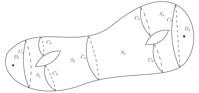
Figure 6: Two torus with two punctures.

We shall now turn this qualitative description of on-shell and off-shell amplitudes into fully quantitative description. Our first task will be to introduce a coordinate system on $\widetilde{\cal P}_{g,m,n}$. It is easy to see that given a Riemann surface of genus $g$ and $m+n$ punctures, we can regard this as a union of $m+n$ disks $\{D_{a}\}$, one around each puncture, and $2g-2+m+n$ spheres $\{S_{i}\}$, each with three holes, joined along $3g-3+2m+2n$ circles $\{C_{s}\}$. An example of this for $m+n=2$ and $g=2$ has been shown in Fig. 6. Let $w_{a}$ denote the choice of local holomorphic coordinates on $D_{a}$ such that the $a$-th puncture is located at $w_{a}=0$ and $z_{i}$ denote the local holomorphic coordinates on $S_{i}$. Then the Riemann surface is prescribed completely by specifying the spin structure and the functional relation between the coordinates on the two sides of each overlap circle $C_{s}$. This typically takes the form

$$z_{i}=f_{ij}(z_{j})\quad\hbox{or}\quad z_{i}=g_{ia}(w_{a})\,.$$ (2.27)

In order to use a compact notation, we shall fix some orientation for each $C_{s}$ and call $\sigma_{s}$ and $\tau_{s}$ respectively the coordinate systems on the left and right of $C_{s}$. Each $\sigma_{s}$ and $\tau_{s}$ will correspond to one of the $z_{i}$ or one of the $w_{a}$. Eq. (2.27) may now be reexpressed as

$$\sigma_{s}=F_{s}(\tau_{s})\,.$$ (2.28)

Besides the spin structure, the functions $\{F_{s}\}$ contain complete information about the Riemann surface and the local coordinate system around the punctures (which are taken to be $w_{a}$). Therefore they can be chosen to parametrize $\widehat{\cal P}_{g,m,n}$. More specifically, if $\{u_{i}\}$ denote the complete set of parameters labelling the functions $\{F_{s}\}$, e.g. coefficients of Laurent series expansion of these functions, then we can take $\{u_{i}\}$ to be the coordinates of $\widehat{\cal P}_{g,m,n}$. This is clearly an infinite dimensional space. Once the coordinate system on $\widehat{\cal P}_{g,m,n}$ is fixed this way, we can introduce coordinate system on $\widetilde{\cal P}_{g,m,n}$ by appending to the former the locations of the PCOs. This introduces one complex coordinate for each PCO. If a PCO is located on $S_{i}$ then we shall specify its coordinate in the $z_{i}$ coordinate system while if it is located on $D_{a}$ we shall specify its location in the $w_{a}$ coordinate system. We shall denote collectively by $\{y_{\alpha}\}$ the locations of all the PCOs. We shall take the NS vertex operators to have picture number $-1$ and the R-vertex operators to have picture number $-1/2$. Then by picture number conservation we need precisely $2g-2+m+n/2$ PCOs for non zero correlation functions.

The set $\{u_{j},y_{\alpha}\}$ provides a highly redundant coordinate system on $\widetilde{\cal P}_{g,m,n}$, since a reparametrization of $z_{i}$ that is non-singular on $S_{i}$ (with the holes cut out) changes the function $F_{s}$ (and hence some of the $u_{j}$’s) if $C_{s}$ forms a boundary of $S_{i}$. This also changes the coordinate $y_{\alpha}$ of a PCO if it is situated on $S_{i}$. On the other hand such a reparametrization does not change the Riemann surface or the local coordinates around the punctures or the physical location of the PCO. Therefore we must identify points in the $\{u_{j},y_{\alpha}\}$ space related by such reparametrizations. A reparametrization of $w_{a}$ that is non-singular inside $D_{a}$ and leaves the location of the puncture $w_{a}=0$ unchanged, changes the local coordinate around the $a$-th puncture but does not change the Riemann surface. Therefore this moves us along the fiber of $\widetilde{\cal P}_{g,m,n}$. However, if this transformation is a phase rotation of $w_{a}$ then it does not have any action on $\widetilde{\cal P}_{g,m,n}$ and again we must identify points in the $\{u_{j},y_{\alpha}\}$ space related by such reparametrizations.

The tangent vectors of $\widetilde{\cal P}_{g,m,n}$ are associated with infinitesimal motions in $\widetilde{\cal P}_{g,m,n}$. One set of tangent vectors, associated with the changes in the PCO locations keeping moduli and local coordinates fixed, are simply $\partial/\partial y_{\alpha}$. The other tangent vectors $\partial/\partial u_{i}$, which are also tangent vectors of $\widehat{\cal P}_{g,m,n}$, are associated with deformation of the transition functions $F_{s}$. For later use we define

$${\bf B}\left[{\partial\over\partial u_{i}}\right]\equiv\sum_{s}\ointop_{C_{s}}{\partial F_{s}\over\partial u_{i}}d\sigma_{s}\,b(\sigma_{s})+\sum_{s}\ointop_{C_{s}}{\partial\bar{F}_{s}\over\partial u_{i}}d\bar{\sigma}_{s}\,\bar{b}(\bar{\sigma}_{s})\,,$$ (2.29)

where $\ointop$ includes a factor of $1/2\pi i$ for the first integral and $-1/2\pi i$ for the second integral. $b$, $\bar{b}$ are the usual ghost fields of the world-sheet theory. By definition, the contour traverses $C_{s}$ keeping the patch covered by the $\sigma_{s}$ coordinate system to the left. It is easy to verify that this definition is invariant under the reversal of the orientation of $C_{s}$ that exchanges $\sigma_{s}$ and $\tau_{s}$.

Suppose we want to compute an off-shell amplitude of $m$ NS sector vertex operators $K_{1},\ldots,K_{m}\in{\cal H}_{-1}$ and $n$ R sector vertex operators $L_{1},\ldots,L_{n}\in{\cal H}_{-1/2}$. In order to avoid some cumbersome sign factors we shall from now on multiply each Grassmann odd vertex operator by a Grassmann odd c-number so that the vertex operators of external states are always Grassmann even. In any equation we can always strip off these Grassmann odd c-numbers from both side to recover the necessary sign factors. We now describe the construction of a $p$-form $\Omega^{(g,m,n)}_{p}(\{K_{i}\},\{L_{j}\})$ on $\widetilde{\cal P}_{g,m,n}$ that can be integrated over a $p$-dimensional subspace of $\widetilde{\cal P}_{g,m,n}$ – henceforth referred to as an integration cycle. This is defined by specifying the contraction of this $p$-form with $p$ arbitrary tangent vectors of $\widetilde{\cal P}_{g,m,n}$ which could be either of the type $\partial/\partial y_{\alpha}$ or of type $\partial/\partial u_{j}$. Denoting by $\Omega^{(g,m,n)}_{p}(\{K_{i}\},\{L_{j}\})\left[\partial/\partial u_{j_{1}},\ldots\partial/\partial u_{j_{k}},\partial/\partial y_{\alpha_{k+1}},\ldots\partial/\partial y_{\alpha_{p}}\right]$ the contraction of the $p$-form with such vector fields, evaluated at some particular point in $\widetilde{\cal P}_{g,m,n}$, we take

$$\Omega^{(g,m,n)}_{p}(\{K_{i}\},\{L_{j}\})\left[\partial/\partial u_{j_{1}},\ldots,\partial/\partial u_{j_{k}},\partial/\partial y_{\alpha_{k+1}},\ldots,\partial/\partial y_{\alpha_{p}}\right]$$ (2.30)

$$= (-2\pi i)^{-(3g-3+m+n)}\Bigg{\langle}{\bf B}[\partial/\partial u_{j_{1}}]\ldots{\bf B}[\partial/\partial u_{j_{k}}](-\partial\xi(y_{\alpha_{k+1}})\ldots(-\partial\xi(y_{\alpha_{p}}))$$

$$\hskip 72.26999pt\prod_{\alpha=1\atop\alpha\neq\alpha_{k+1},\ldots\alpha_{p}}^{2g-2+m+n/2}{\cal X}(y_{\alpha})\,K_{1}\ldots K_{m}L_{1}\ldots L_{n}\Bigg{\rangle}_{\Sigma_{g,m,n}}\,.$$

We shall now explain the various parts of this formula. First of all this expression gives the contraction of the $p$-form with the vector fields at some particular point in $\widetilde{\cal P}_{g,m,n}$. Associated with this point there is a specific Riemann surface $\Sigma_{g,m,n}$ with $m+n$ punctures, local coordinates at each of these punctures and choice of PCO locations on the Riemann surface. $y_{1},\ldots,y_{2g-2+m+n/2}$ denote these PCO locations. $\langle\cdots\rangle_{\Sigma_{g,m,n}}$ denotes correlation function on the Riemann surface $\Sigma_{g,m,n}$. The actual computation of these correlation functions require detailed knowledge of the underlying SCFT. For simple background, explicit expressions of these correlation functions can be found e.g. in [104, 105]. The vertex operators $\{K_{i}\}$ and $\{L_{j}\}$ are inserted at the punctures of the Riemann surface using the chosen local coordinates corresponding to the particular point in $\widetilde{\cal P}_{g,m,n}$ where we want to compute the left hand side. ${\bf B}[\partial/\partial u_{j}]$ has been defined in (2.29).

The expression (LABEL:edefomega) clearly depends on the choice of the PCO locations $y_{\alpha}$. It also depends on the choice of local coordinates around the punctures. For example, if $K_{a}$ is a primary operator of dimension $(h,h)$ inserted at the $a$-th puncture at $w_{a}=0$, then under a change in local coordinates from $w_{a}$ to $\widetilde{w}_{a}=f(w_{a})$, the correlator is multiplied by a factor of $|f^{\prime}(0)|^{-2h}$. For non-primary states the transformation law is more complicated, involving mixing with other descendants of the primary. Since the local coordinates around the punctures are defined only up to a phase rotation, (LABEL:edefomega) is well defined only if the external states are annihilated by $L_{0}^{-}$; otherwise a phase rotation of the local coordinates will change the correlation function.

The above definition of $\Omega^{(g,m,n)}_{p}$ may look somewhat formal since $\widetilde{\cal P}_{g,m,n}$ is an infinite dimensional space parametrized by infinite number of coordinates $\{u_{i},y_{\alpha}\}$. For any practical computation we shall integrate $\Omega^{(g,m,n)}_{p}$ over a given $p$-dimensional subspace with fixed set of tangent vectors. In this case (LABEL:edefomega) can be used to find a specific $p$-form on this $p$ dimensional subspace of $\widetilde{\cal P}_{g,m,n}$ as follows. Let us suppose that $t_{1},\ldots t_{p}$ denote the parameters that label the $p$ dimensional subspace of $\widetilde{\cal P}_{g,m,n}$. Then in general all the transition functions $F_{s}$ and the PCO locations $\{y_{\alpha}\}$ will depend on the parameters $\{t_{i}\}$. According to (2.29), (LABEL:edefomega), contraction of $\Omega^{(g,m,n)}_{p}$ with a tangent vector $\partial/\partial t_{i}$ will correspond to inserting the operator

$${\cal B}_{i}=\sum_{s}\ointop_{C_{s}}{\partial F_{s}\over\partial t_{i}}d\sigma_{s}\,b(\sigma_{s})+\sum_{s}\ointop_{C_{s}}{\partial\bar{F}_{s}\over\partial t_{i}}d\bar{\sigma}_{s}\,\bar{b}(\bar{\sigma}_{s})-\sum_{\alpha}{1\over{\cal X}(y_{\alpha})}{\partial y_{\alpha}\over\partial t_{i}}\partial\xi(y_{\alpha})$$ (2.31)

into the correlation function. Note the formal factor of $1/{\cal X}(y_{\alpha})$ – this simply means that we have to remove the ${\cal X}(y_{\alpha})$ factor from the rest of the operator insertion. The net integration measure will be given by

$$(-2\pi i)^{-(3g-3+m+n)}\left\langle{\cal B}_{1}dt_{1}\wedge{\cal B}_{2}dt_{2}\wedge\ldots\wedge{\cal B}_{p}dt_{p}\,\prod_{\alpha=1}^{2g-2+m+n/2}{\cal X}(y_{\alpha})\,K_{1}\ldots K_{m}L_{1}\ldots L_{n}\right\rangle_{\Sigma_{g,m,n}}\,.$$ (2.32)

This has no ${\cal X}(y_{\alpha})$ in the denominator since the same $1/{\cal X}(y_{\alpha})$ given in (2.31) cannot appear more than once due to the vanishing of the corresponding wedge product $\partial_{t_{1}}y^{\alpha}dt_{1}\wedge\partial_{t_{2}}y^{\alpha}dt_{2}$. Single factors of ${\cal X}(y_{\alpha})$ in the denominator get cancelled by the $\prod_{\alpha=1}^{2g-2+m+n/2}{\cal X}(y_{\alpha})$ factor. We emphasize again that the ${\cal X}(y_{\alpha})$ in the denominator of (2.31) is only a formal way of writing the final expression.

The $p$-form defined in (LABEL:edefomega) has several useful properties:

1. First of all recall that the coordinate system on $\widetilde{\cal P}_{g,m,n}$ that we have used is highly redundant. Consequently there are many vectors which actually represent zero vectors of $\widetilde{\cal P}_{g,m,n}$. Examples of such tangent vectors are those generated by infinitesimal reparametrization of $z_{i}$ together with a shift of the PCO locations on $S_{i}$ that keeps their physical location unchanged. Such tangent vectors will be represented by some linear combination of the vectors $\partial/\partial u_{j}$ and $\partial/\partial y^{\alpha}$. We need to ensure that the contraction of $\Omega^{(g,m,n)}_{p}$ with such vectors must vanish since they represent zero tangent vector. We shall now show that this can be proved using standard properties of correlation functions of conformal field theories on Riemann surfaces.

   For definiteness, suppose that we make an infinitesimal deformation of the coordinate system $z_{1}$ on $S_{1}$ to $z_{1}+v(z_{1})$. Let us suppose further that $C_{1}$, $C_{2}$ and $C_{3}$ form boundaries of $S_{1}$ keeping $S_{1}$ on the left, and that on $S_{1}$ there are insertions of PCOs at $y_{1},\ldots y_{N}$. Then on $C_{s}$ for $1\leq s\leq 3$, $F_{s}$ changes by $v(z_{1})$, and for $1\leq\alpha\leq N$, $y_{\alpha}$ changes by $v(y_{\alpha})$. The relevant insertion into the correlation function upon contraction of $\Omega^{(g,m,n)}_{p}$ with the tangent vector induced by this deformation takes the form

   $$\left[\sum_{i=1}^{3}\ointop_{C_{i}}v(z_{1})b(z_{1})dz_{1}+\sum_{i=1}^{3}\ointop_{C_{i}}\bar{v}(\bar{z}_{1})\bar{b}(\bar{z}_{1})d\bar{z}_{1}\right]\prod_{\beta=1}^{N}{\cal X}(y_{\beta})-\sum_{\alpha=1}^{N}(v(y_{\alpha})\partial\xi(y_{\alpha}))\prod_{\beta=1\atop\beta\neq\alpha}^{N}{\cal X}(y_{\beta})\,,$$ (2.33)

   with the integration along $C_{1},C_{2},C_{3}$ performed by keeping $S_{1}$ to the left. We can now deform the integration contours into the interior of $S_{1}$. The contour integral over $\bar{z}_{1}$ can be shrunk to a point giving vanishing contribution, while the integral over $z_{1}$ picks up residues at $y_{\alpha}$ due to the insertion of ${\cal X}(y_{\alpha})$. It follows from (2.13) that these residues are given by $v(y_{\alpha})\partial\xi(y_{\alpha})$. The sum of all the residues cancel the last term. Therefore we see that the apparent tangent vector induced by a change of coordinate on $S_{1}$ indeed has vanishing contraction with $\Omega^{(g,m,n)}_{p}$.

2. Similarly contraction of $\Omega^{(g,m,n)}_{p}$ with tangent vectors associated with phase rotation $w_{a}\to w_{a}+i\epsilon w_{a}$ of the $w_{a}$’s can also be shown to vanish. If there are $M$ insertions of PCOs at $y_{1},\ldots y_{M}$ on $D_{a}$ then the relevant insertion upon contraction with the corresponding tangent vector takes the form

   $$\left[i\epsilon\ointop_{C_{a}}w_{a}b(w_{a})dw_{a}-i\epsilon\ointop_{C_{a}}\bar{w}_{a}\bar{b}(\bar{w}_{a})d\bar{w}_{a}\right]\prod_{\beta=1}^{M}{\cal X}(y_{\beta})V_{a}(0)$$

   $$-i\epsilon\sum_{\alpha=1}^{M}(y_{\alpha}\partial\xi(y_{\alpha}))\prod_{\beta=1\atop\beta\neq\alpha}^{M}{\cal X}(y_{\beta})V_{a}(0)\,,$$ (2.34)

   where $C_{a}$ represents an anti-clockwise contour along the boundary of the disk $D_{a}$ around the $a$-th puncture, and $V_{a}$ is the vertex operator inserted at the $a$-th puncture at $w_{a}=0$. We can now deform the contour $C_{a}$ towards $w_{a}=0$. Sum of the residues at $y_{\alpha}$ cancel the last term as before, leaving us with the residue at $w_{a}=0$. This is proportional to $b_{0}^{-}|V_{a}\rangle$ and vanishes by eq. (2.16) since $V_{a}\in{\cal H}_{T}$.

3. $\Omega^{(g,m,n)}_{p}$ satisfies the important identity

   $$\Omega^{(g,m,n)}_{p}(Q_{B}K_{1},K_{2},\ldots,K_{m},L_{1},\ldots,L_{n})+\cdots+\Omega^{(g,m,n)}_{p}(K_{1},K_{2},\ldots,K_{m},L_{1},\ldots,Q_{B}L_{n})$$ (2.35)

   $$= (-1)^{p}d\Omega^{(g,m,n)}_{p-1}(K_{1},\ldots,K_{m},L_{1},\ldots,L_{n})\,.$$

   The derivation of this formula can be found in [99]. We shall not repeat it here with all the details but briefly indicate the general idea behind the proof. Let us pick some convenient coordinate system $\{u_{i}\}$ on $\widehat{\cal P}_{g,m,n}$, and use $\{u_{i}\}$ and the PCO locations $\{y_{\alpha}\}$ as the coordinates of $\widetilde{\cal P}_{g,m,n}$. We now take the contraction of both sides of (LABEL:emm) with $q$ tangent vectors of the form $\partial/\partial u_{i}$ and $p-q$ tangent vectors of the form $\partial/\partial y_{\alpha}$, and evaluate both sides using (LABEL:edefomega). Since on the left hand side we have $Q_{B}$ acting on all the states in turn, we can deform the contour of integration defining $Q_{B}$ into the interior of the Riemann surface, picking up residues from the insertions of $b,\bar{b}$ ghosts in the $B[\partial/\partial u_{i}]$ factors and also from the $\partial\xi$ insertions. ${\cal X}$ insertions of course are invariant under $Q_{B}$. One might also worry about possible residues from the spurious poles mentioned at the end of §2.1, but as has been reviewed in appendix C, there are no spurious poles in the argument of the BRST current[106, 107]. Using the relations

   $$\{Q_{B},b(z)\}=T(z),\quad\{Q_{B},\bar{b}(\bar{z})\}=\bar{T}(\bar{z})\,,$$ (2.36)

   where $\bar{T}$ and $T$ are the left- and right-moving components of the total stress tensor of the world-sheet theory, we can see that the residue at $B[\partial/\partial u_{i}]$ generates a factor similar to that in (2.29) with $b,\bar{b}$ replaced by stress tensors $T,\bar{T}$. This generates derivative of the correlation function with respect to $u_{i}$. On the other hand the residue at $\partial\xi(y_{\alpha})$ generates a factor of $\partial{\cal X}(y_{\alpha})$ and this generates derivative of the correlation function with respect to the coordinate $y_{\alpha}$. Putting all these results together one finds that the contraction of the left and right hand sides of (LABEL:emm) with arbitrary set of tangent vectors agrees. This establishes (LABEL:emm).

4. Since on a genus $g$ surface we need total ghost number $6-6g$ to get a non-zero correlator, we see that $\Omega^{(g,m,n)}_{p}(\{K_{i}\},\{L_{j}\})$ is non-zero only if the total ghost number carried by $\{K_{i}\}$ and $\{L_{j}\}$ is equal to $6-6g+p$. On the other hand conservation of picture number is automatic due to our choice of picture numbers of $\{K_{i}\}$ and $\{L_{j}\}$, and the number of PCO insertions in the definition of $\Omega^{(g,m,n)}_{p}(\{K_{i}\},\{L_{j}\})$.

We are now ready to define off-shell amplitudes. The off-shell amplitude of the external states $K_{1},\ldots,K_{m},L_{1},\ldots,L_{n}$ is given by

$$\int_{{\cal S}_{g,m,n}}\Omega^{(g,m,n)}_{6g-6+2m+2n}(K_{1},\ldots,K_{m},L_{1},\ldots,L_{n})\,,$$ (2.37)

where ${\cal S}_{g,m,n}$ is a section of $\widetilde{\cal P}_{g,m,n}$. For on-shell external states this gives the usual on-shell amplitudes and can be shown to be formally independent of the choice of ${\cal S}_{g,m,n}$. The proof of this has been reviewed in §2.3. However for off-shell external states the result depends on the choice of this section since the external states are not BRST invariant. We shall describe in §5.4 and appendix E how physical quantities computed from off-shell amplitudes become independent of the choice of the section.

As already mentioned in footnote 6, we cannot choose the section to be continuous, but once we add correct compensating terms we can treat it as continuous in all manipulations. We can further generalize the notion of a section by taking weighted averages of sections – several sections ${\cal S}^{(1)}_{g,m,n},\ldots{\cal S}^{(k)}_{g,m,n}$ with weights $w_{1},\ldots w_{k}$ such that $\sum_{i=1}^{k}w_{i}=1$. If we denote by ${\cal S}_{g,m,n}$ the formal weighted sum $\sum_{i=1}^{k}w_{i}\,{\cal S}^{(i)}_{g,m,n}$ then by definition

$$\int_{{\cal S}_{g,m,n}}\Omega^{(g,m,n)}_{6g-6+2m+2n}(K_{1},\ldots,K_{m},L_{1},\ldots,L_{n})=\sum_{i=1}^{k}w_{i}\int_{{\cal S}^{(i)}_{g,m,n}}\Omega^{(g,m,n)}_{6g-6+2m+2n}(K_{1},\ldots,K_{m},L_{1},\ldots,L_{n})\,.$$ (2.38)

This is also a good definition of off-shell amplitude since for on-shell external states the result reduces to the usual on-shell amplitude. We shall call sections of this kind ‘generalized sections’. In all subsequent analysis whenever we refer to section, we shall actually mean generalized section.

Some explicit examples of off-shell amplitudes computed using this prescription can be found in appendix B.

The story in type II string theory is similar. For an amplitude with $m$ NSNS states, $n$ NSR states, $r$ RNS states and $s$ RR states one has to work with the space $\widetilde{\cal P}_{g,m,n,r,s}$ which has as its fiber the choice of local coordinates at the punctures and locations of $m+n+(r+s)/2$ left-moving PCOs and $m+r+(n+s)/2$ right-moving PCOs. Construction of $\Omega^{(g,m,n,r,s)}_{p}$ proceeds in a manner identical to that of heterotic string theory, with the contraction with tangent vectors $\partial/\partial\tilde{y}_{\alpha}$, with $\tilde{y}_{\alpha}$ denoting the location of the left-moving PCO, introducing a factor of $-\bar{\partial}\bar{\xi}(\tilde{y}_{\alpha})$.

2.3 Formal properties of on-shell amplitudes

Using (LABEL:emm) we can prove some useful formal properties of on-shell amplitudes[103], where an on-shell state will refer to a state that is BRST invariant, but not necessarily a dimension zero primary. First consider the situation where all the states $K_{1},\ldots,K_{m}$, $L_{1},\ldots,L_{n}$ are BRST invariant and one of them, say $K_{1}$, is BRST exact, i.e. $K_{1}=Q_{B}\Lambda$. Then using (LABEL:emm) we get

$$\Omega^{(g,m,n)}_{6g-6+2m+2n}(Q_{B}\Lambda,K_{2},\ldots,K_{m},L_{1},\ldots,L_{n})=d\Omega^{(g,m,n)}_{6g-6+2m+2n-1}(\Lambda,K_{2},\ldots,K_{m},L_{1},\ldots,L_{n})\,.$$ (2.39)

We now integrate both sides over ${\cal S}_{g,m,n}$. The left hand side gives the on-shell amplitude in which one state is BRST exact. The right hand side is the integral of an exact form and hence the integral vanishes provided we can ignore the boundary terms. This shows the decoupling of pure gauge states. We emphasize however that this ‘derivation’ is formal since it ignores possible contribution from the boundary terms. One of our goals will be to give a complete proof of the decoupling of pure gauge states with the help of superstring field theory, without having to worry about potential boundary contributions.

Figure 7: The region ${\cal U}_{g,m,n}$ interpolating between two sections ${\cal S}_{g,m,n}$ and ${\cal S}^{\prime}_{g,m,n}$.The subspace ${\cal V}_{g,m,n}$ is part of the fiber of $\widetilde{\cal P}_{g,m,n}$ over the boundary of ${\cal M}_{g,m,n}$. We shall choose the orientation of ${\cal S}^{\prime}_{g,m,n}$ and ${\cal V}_{g,m,n}$ to be outward from ${\cal U}_{g,m,n}$ and that of ${\cal S}_{g,m,n}$ to be inward towards ${\cal U}_{g,m,n}$.

Next we shall consider the dependence of the on-shell amplitudes on the choice of the section ${\cal S}_{g,m,n}$. For this we again consider a set of BRST invariant states $K_{1},\ldots K_{m}$, $L_{1},\ldots L_{n}$. The genus $g$ amplitudes of these states is given by (2.37). Now if we choose a different section ${\cal S}^{\prime}_{g,m,n}$ then it is possible to find a dimension $6g-6+2(m+n)+1$ subspace ${\cal U}_{g,m,n}$ that interpolates between ${\cal S}_{g,m,n}$ and ${\cal S}^{\prime}_{g,m,n}$. Of course ${\cal U}_{g,m,n}$ is not determined uniquely. In this case we have

$$\partial{\cal U}_{g,m,n}={\cal S}^{\prime}_{g,m,n}-{\cal S}_{g,m,n}+{\cal V}_{g,m,n}\,,$$ (2.40)

where ${\cal V}_{g,m,n}$ denotes the intersection of ${\cal U}_{g,m,n}$ with the fiber over the boundary of ${\cal M}_{g,m,n}$. This has been shown pictorially in Fig. 7. We now get

$$\displaystyle\int_{{\cal S}^{\prime}_{g,m,n}}\Omega^{(g,m,n)}_{6g-6+2(m+n)}-\int_{{\cal S}_{g,m,n}}\Omega^{(g,m,n)}_{6g-6+2(m+n)} = \int_{{\cal U}_{g,m,n}}d\Omega^{(g,m,n)}_{6g-6+2(m+n)}-\int_{{\cal V}_{g,m,n}}\Omega^{(g,m,n)}_{6g-6+2(m+n)}$$ (2.41)

$$= -\int_{{\cal V}_{g,m,n}}\Omega^{(g,m,n)}_{6g-6+2(m+n)}\,.$$

where in the last step we have used the fact that $d\Omega^{(g,m,n)}_{6g-6+2(m+n)}$ with BRST invariant arguments vanishes due to (LABEL:emm). Therefore we see that the difference between the on-shell amplitudes computed using the two sections vanishes up to boundary terms. We shall see in §5.4 and appendix E that once on-shell amplitudes are defined using superstring field theory, the result can be shown to be independent of the choice of sections without having to make any assumption about the vanishing of the boundary terms.

3 Superstring field theory: Gauge fixed action

A field theory of superstrings will produce off-shell amplitudes but not all off-shell amplitudes may have field theory interpretation. In order to have a field theory interpretation the off-shell amplitude must be expressed as the contribution from a sum of Feynman diagrams. Therefore the section ${\cal S}_{g,m,n}$ must admit a cell decomposition with each cell describing a section over a codimension zero subspace of ${\cal M}_{g,m,n}$, such that

• the integral of $\Omega^{(g,m,n)}_{6g-6+2m+2n}$ over a given cell can be interpreted as the contribution from one particular Feynman diagram of superstring field theory, and

• the sum of the contribution from all the cells has the interpretation of the sum over all the Feynman diagrams.

We shall now describe under what conditions this holds. From now on we shall refer to the segments of ${\cal S}_{g,m,n}$ corresponding to individual Feynman diagrams as section segments of the corresponding Feynman diagrams.

3.1 Condition on the choice of sections

One of the key properties of Feynman diagrams is that a pair of Feynman diagrams can be joined by a propagator to make a new Feynman diagram. A related property is that two external legs of a single Feynman diagram can be joined to make a new Feynman diagram with an additional loop. Now, each Feynman diagram of superstring field theory is expected to correspond to an integral of $\Omega$ over a section segment. This means that there must be an operation that takes the section segments of two different Feynman diagrams and gives the section segment of the new Feynman diagram obtained by joining the two by a propagator. There must also be another operation which acts on the section segment of a single Feynman diagram and generates a section segment of the new Feynman diagram obtained by joining two external legs of the original Feynman diagram. Our first task will be to describe these operations. Again for simplicity of notation, we restrict our analysis to heterotic string theories; the analysis for type II string theories is more or less identical.

For reasons that will become clear in due course, the operation of joining two legs of two different Feynman diagrams or two legs of the same Feynman diagram, is played by an operation on Riemann surfaces known as plumbing fixture. First recall that for each external leg of a Feynman diagram we have a puncture on the corresponding Riemann surface, and that for a given choice of section segment, we also have a choice of local coordinates at the punctures and the PCO locations on the Riemann surface. The operation of joining a pair of external legs of a Feynman diagram (or of two Feynman diagrams) will be represented by the operation of identifying the local coordinates $w_{1}$ and $w_{2}$ around the corresponding punctures via the relation

$$w_{1}w_{2}=e^{-s-i\theta},\quad 0\leq s<\infty,\quad 0\leq\theta<2\pi\,.$$ (3.1)

This is known as the operation of sewing the regions around the punctures to each other since as we traverse towards $w_{1}\to 0$ we emerge in the $w_{2}$ plane away from 0. This also induces local coordinates around the punctures of the new Riemann surface[109, 110, 111] and PCO locations on the new Riemann surface from those on the original surfaces that are being sewed. We shall now verify that the new family of Riemann surfaces generated by this way satisfies the properties that are required to be satisfied by the section segment of a new Feynman diagram obtained by joining two legs of the same Feynman diagram or two legs of two different Feynman diagrams.

If the punctures that are being sewed lie on two different Riemann surfaces $\Sigma_{g_{1},m_{1},n_{1}}$ and $\Sigma_{g_{2},m_{2},n_{2}}$, then for given $s$, $\theta$ plumbing fixture generates a new Riemann surface $\Sigma_{g_{1}+g_{2},m_{1}+m_{2}-2,n_{1}+n_{2}}$ if the punctures are NS punctures, i.e. they have NS sector vertex operators inserted. Similarly, the sewing process generates a new Riemann surface $\Sigma_{g_{1}+g_{2},m_{1}+m_{2},n_{1}+n_{2}-2}$ if the punctures that are being sewed are R punctures. When we sew the regions around two punctures on the same Riemann surface $\Sigma_{g,m,n}$, the result is a new Riemann surface $\Sigma_{g+1,m-2,n}$ or $\Sigma_{g+1,m,n-2}$. In all cases this operation also generates local coordinate systems around the punctures of the new Riemann surface and the PCO locations on the new Riemann surface from those on the original Riemann surface(s). There is a slight subtlety in the case of sewing R punctures that we shall illustrate using the case of sewing two different Riemann surfaces. If we consider two Riemann surfaces $\Sigma_{g_{1},m_{1},n_{1}}$ and $\Sigma_{g_{2},m_{2},n_{2}}$, then the total number of PCOs is given by

$$\displaystyle 2g_{1}-2+m_{1}+{n_{1}\over 2} + 2g_{2}-2+m_{2}+{n_{2}\over 2}$$ (3.2)

$$= 2(g_{1}+g_{2})-2+(m_{1}+m_{2}-2)+{n_{1}+n_{2}\over 2}$$

$$= 2(g_{1}+g_{2})-2+(m_{1}+m_{2})+{n_{1}+n_{2}-2\over 2}-1\,.$$

The equality in the second line shows that the number on the left hand side is precisely equal to the required number of PCOs on $\Sigma_{g_{1}+g_{2},m_{1}+m_{2}-2,n_{1}+n_{2}}$. However equality in the third line shows that the number on the left is one less than the required number of PCOs on $\Sigma_{g_{1}+g_{2},m_{1}+m_{2},n_{1}+n_{2}-2}$. In other words when the sewing is done at the R punctures, we need to insert an extra PCO on the final surface. We shall use the symmetric prescription that the new PCO location is taken to be the average over a circle around one of the punctures, i.e. we insert

$$\ointop{dw_{1}\over w_{1}}{\cal X}(w_{1})=\ointop{dw_{2}\over w_{2}}{\cal X}(w_{2})\,,$$ (3.3)

where $\ointop$ includes a factor of $1/2\pi i$ and the integration is carried out over an anti-clockwise contour. The equality of the two terms in this equation follows from (3.1) and the fact that ${\cal X}$ is a dimension zero primary operator. A similar analysis involving sewing two punctures on the same Riemann surface shows that we need a similar insertion when the punctures that are sewed carry Ramond sector vertex operators. Note that for sewing R punctures this requirement automatically makes the final section a generalized section in the sense described in (2.38), since the extra PCO insertion, instead of being at a single point, is taken to be an average over a continuous family as given in (3.3).

Now a Feynman diagram does not represent a single Riemann surface but a whole family of Riemann surfaces belonging to the section segment of the Feynman diagram. Therefore given two Feynman diagrams, we can get a subspace of $\widetilde{\cal P}_{g_{1}+g_{2},m_{1}+m_{2}-2,n_{1}+n_{2}}$ or $\widetilde{\cal P}_{g_{1}+g_{2},m_{1}+m_{2},n_{1}+n_{2}-2}$ by plumbing fixture of all Riemann surfaces corresponding to the first Feynman diagram to all Riemann surfaces of the second Feynman diagram. The resulting subspace has dimension

$$6g_{1}-6+2m_{1}+2n_{1}+6g_{2}-6+2m_{2}+2n_{2}+2=6(g_{1}+g_{2})-6+2(m_{1}+m_{2}+n_{1}+n_{2}-2)\,.$$ (3.4)

The last additive factor of 2 on the left hand side comes from the parameters $(s,\theta)$. We shall refer to this operation as plumbing fixture of two section segments. The right hand side of (3.4) is precisely the required dimension of a section of $\widetilde{\cal P}_{g_{1}+g_{2},m_{1}+m_{2}-2,n_{1}+n_{2}}$ and $\widetilde{\cal P}_{g_{1}+g_{2},m_{1}+m_{2},n_{1}+n_{2}-2}$. Therefore we see that it is consistent to interpret this subspace of $\widetilde{\cal P}_{g_{1}+g_{2},m_{1}+m_{2}-2,n_{1}+n_{2}}$ or $\widetilde{\cal P}_{g_{1}+g_{2},m_{1}+m_{2},n_{1}+n_{2}-2}$ as the section segment of the new Feynman diagram obtained by joining the original Feynman diagrams by a propagator. A similar analysis shows that when we generate a new Feynman diagram by joining two of the legs of a Feynman diagram by a propagator, it is consistent to interpret the family of Riemann surfaces, obtained by the plumbing fixture of the section segment of the original diagram at two of its punctures, as the section segment of the new Feynman diagram. Once we have chosen this interpretation, the section segments of all Feynman diagrams are obtained from the section segments of Feynman diagrams containing a single interaction vertex and no internal propagators via repeated operation of plumbing fixture. We shall denote by ${\overline{{\cal R}}}_{g,m,n}$ the section segments of Feynman diagrams containing a single interaction vertex and no internal propagators, contributing to a genus $g$ amplitude with $m$ external NS sector states and $n$ external R sector states. To simplify notation, we shall often refer to them as section segments of the interaction vertices of superstring field theory. Of course, the requirement that the sum of the section segments of different Feynman diagrams generates a full (generalized) section ${\cal S}_{g,m,n}$ puts strong restriction on the choice of ${\overline{{\cal R}}}_{g,m,n}$.

The $s\to\infty$ limit in (3.1) describes degenerate Riemann surface. We shall see in §3.4 that the parameter $s$ plays the role of the Schwinger parameter $s$ appearing in (1.2) in quantum field theory. Therefore we see that the type 1 and type 2 divergences discussed in §1 are both associated with degenerate Riemann surfaces.

We shall now outline a systematic algorithm for generating section segments satisfying these requirements, generalizing the corresponding algorithm for bosonic string field theory[33]. We begin with the section segments of genus zero three point interaction vertex – they are appropriate subspaces of $\widetilde{\cal P}_{0,3,0}$ and $\widetilde{\cal P}_{0,1,2}$. Since the base is zero dimensional, they just represent a point on the fiber. They have to be chosen such that they are symmetric under the exchange of the punctures, e.g. for NS-NS-NS vertex an SL(2,C) transformation exchanging a pair of punctures should exchange the corresponding local coordinates and leave the PCO location unchanged. This will encode another important property of a Feynman diagram, i.e. a Feynman diagram containing a single interaction vertex and no internal propagators is symmetric under the exchange of external legs. Typically this will require averaging over the choice of PCO locations, i.e. using generalized sections. Furthermore these section segments must avoid spurious poles. For $\widetilde{\cal P}_{0,1,2}$ this condition is trivial since there are no PCO insertions, while for $\widetilde{\cal P}_{0,3,0}$ this condition simply means that the single PCO insertion that is needed should not coincide with any of the punctures. We shall call these section segments ${\overline{{\cal R}}}_{0,3,0}$ and ${\overline{{\cal R}}}_{0,1,2}$ respectively – in this case they also represent the full sections ${\cal S}_{0,3,0}$ and ${\cal S}_{0,1,2}$. Now we can construct the section segments of tree level four point function corresponding to s, t and u-channel diagrams by plumbing fixture of two of the section segments of tree level three point functions. These will be appropriate subspaces of $\widetilde{\cal P}_{0,4,0}$, $\widetilde{\cal P}_{0,2,2}$ or $\widetilde{\cal P}_{0,0,4}$. These together will not, in general, give full sections of $\widetilde{\cal P}_{0,4,0}$, $\widetilde{\cal P}_{0,2,2}$ and $\widetilde{\cal P}_{0,0,4}$. We fill the gap by section segments ${\overline{{\cal R}}}_{0,4,0}$, ${\overline{{\cal R}}}_{0,2,2}$ and ${\overline{{\cal R}}}_{0,0,4}$ and interpret them as the section segments of the elementary four point interaction vertices. This has been shown schematically in Fig. 8. Again we have to construct them avoiding spurious poles, maintaining exchange symmetry and the requirement that at the boundary they join smoothly the section segments of the s, t and u-channel diagrams so that together they describe a smooth section of $\widetilde{\cal P}_{0,m,n}$ for $m+n=4$.

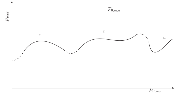
Figure 8: The section of $\widetilde{\cal P}_{0,m,n}$ for the 4 point amplitude at genus 0. The solid lines represent the section segments of the s, t and u-channel diagrams. The dashes lines, which are chosen to ‘fill the gap’, represent the section segment of the elementary four point vertex. While in this one dimensional projection the dashed lines seem to form disconnected sets, typically they form a connected subspace of $\widetilde{\cal P}_{0,m,n}$ when we consider their extension into other directions. Degenerate Riemann surfaces sit in the interior of the solid lines.

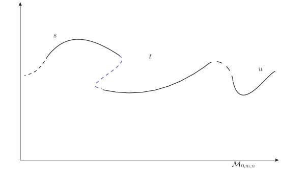
Figure 9: A case where the projection to ${\cal M}_{0,m,n}$ of section segments of s and t-channel diagrams, shown by the solid lines, overlap. We take care of this by joining the end points as shown by dashed line. This effectively removes the overlap portion by adding negative contribution.

Similarly by plumbing fixture of two legs of ${\overline{{\cal R}}}_{0,3,0}$ and ${\overline{{\cal R}}}_{0,1,2}$ we can generate section segments of the one loop tadpole diagram, given by a subspace of $\widetilde{\cal P}_{1,1,0}$. In general this will not generate a full section of $\widetilde{\cal P}_{1,1,.0}$ and we fill the gap by including a section segment ${\overline{{\cal R}}}_{1,1,0}$ which we interpret as the genus 1 contribution to the elementary 1-point vertex of string theory. This procedure can be repeated ad infinitum, generating, for all $g,m,n$, the section segments ${\overline{{\cal R}}}_{g,m,n}$ of the elementary vertices at genus $g$ with $m$ external NS-sector legs and $n$ external R sector legs. At each stage, we first construct the section segments of all the Feynman diagrams obtained by joining lower order vertices by propagators, and then ‘fill the gap’ by appropriate choice of the section segment ${\overline{{\cal R}}}_{g,m,n}$ of the elementary vertex.

An interesting question is: what happens if the section segments of the Feynman diagrams with one or more internal propagators, when projected to ${\cal M}_{g,m,n}$, overlap instead of leaving gaps. Since we have defined the integration measure on $\widetilde{\cal P}_{g,m,n}$, there is in principle no difficulty in filling the gap even in this situation. This has been illustrated in Fig. 9. However we shall see in §3.7 that by ‘adding stubs’ in the definition of interaction vertices it is possible to arrange that the Feynman diagrams containing one or more internal propagators cover only a small part of ${\cal M}_{g,m,n}$ near the boundary of the moduli space. In that case there is no overlap of the kind shown in Fig. 9 in the contribution from different Feynman diagrams.

There is one more constraint that we need to impose on the section segments ${\overline{{\cal R}}}_{g,m,n}$. $\widetilde{\cal P}_{g,m,n}$ admits a ${\hbox{ Z\kern-4.55244ptZ}}_{2}$ action under which all the transition functions $F_{s}$ appearing in (2.28), the local coordinates around the punctures and the PCO locations are complex conjugated. We require ${\overline{{\cal R}}}_{g,m,n}$ to be invariant under this ${\hbox{ Z\kern-4.55244ptZ}}_{2}$ symmetry, i.e. given any point on ${\overline{{\cal R}}}_{g,m,n}$, its ${\hbox{ Z\kern-4.55244ptZ}}_{2}$ image must also be in ${\overline{{\cal R}}}_{g,m,n}$. Again this may require us to average over section segments. This condition on ${\overline{{\cal R}}}_{g,m,n}$ is necessary for establishing reality of the superstring field theory action discussed in §4.4.

A key property of the section segments ${\overline{{\cal R}}}_{g,m,n}$ is that they do not contain any degenerate Riemann surface. Indeed all degenerate Riemann surfaces are associated with Feynman diagrams with at least one propagator, and occur in the limit when the $s$ parameter of the plumbing fixture corresponding to one (or more) of the propagators approaches infinity. For example all degenerate 4-punctured spheres on ${\cal S}_{0,m,n}$ with $m+n=4$ come from s, t and u channel Feynman diagrams, and ${\overline{{\cal R}}}_{0,m,n}$ is free from degenerate 4-punctured spheres.

There is one issue that should still worry us. We have mentioned before that in defining the off-shell amplitudes the sections ${\cal S}_{g,m,n}$ must be chosen to avoid spurious poles. Now since the choice of ${\overline{{\cal R}}}_{g,m,n}$ is up to us, we can follow the procedure of [99, 100] – reviewed in appendix C – to choose them avoiding spurious poles. But now the section segments of Feynman diagrams with one or more propagators are fixed by the section segments ${\overline{{\cal R}}}_{g,m,n}$ of the constituent vertices. Therefore we have to check if these section segments also avoid spurious poles. This issue will be addressed in §3.7 where we shall argue that under certain conditions, once we choose ${\overline{{\cal R}}}_{g,m,n}$ avoiding spurious poles, the section segments of all other Feynman diagrams also avoid spurious poles.

Before concluding this section, we would like to emphasize that there are possible choices of sections of $\widetilde{\cal P}_{g,m,n}$ which violate these conditions. For example we could choose the sections of $\widetilde{\cal P}_{g,m,n}$ arbitrarily without having any relation to each other. Integrating $\Omega^{(g,m,n)}_{6g-6+2m+2n}$ over such sections will define some off-shell amplitudes but they will not have the interpretation as being given by a sum over Feynman diagrams.

3.2 Identities for section segments of interaction vertices

A special role in our analysis will be played by the section segments ${\overline{{\cal R}}}_{g,m,n}$ of the elementary vertices. Therefore we shall now analyze some of the essential properties of ${\overline{{\cal R}}}_{g,m,n}$. As already mentioned, ${\overline{{\cal R}}}_{g,m,n}$ is taken to be symmetric under the exchange of any pair of NS-punctures and also under the exchange of any pair of R-punctures. This needs to be achieved, if necessary, by taking ${\overline{{\cal R}}}_{g,m,n}$ to be formal weighted average of subspaces related by these exchange transformations. Plumbing fixture of ${\overline{{\cal R}}}_{g_{1},m_{1},n_{1}}$ and ${\overline{{\cal R}}}_{g_{2},m_{2},n_{2}}$ at an NS puncture produces a section segment which we shall denote by ${\overline{{\cal R}}}_{g_{1},m_{1},n_{1}}\circ{\overline{{\cal R}}}_{g_{2},m_{2},n_{2}}$. On the other hand, plumbing fixture of ${\overline{{\cal R}}}_{g_{1},m_{1},n_{1}}$ and ${\overline{{\cal R}}}_{g_{2},m_{2},n_{2}}$ at an R puncture produces a section segment which we shall denote by ${\overline{{\cal R}}}_{g_{1},m_{1},n_{1}}\star{\overline{{\cal R}}}_{g_{2},m_{2},n_{2}}$. The information about the insertion of the extra PCO (3.3) will be included in the definition of ${\overline{{\cal R}}}_{g_{1},m_{1},n_{1}}\star{\overline{{\cal R}}}_{g_{2},m_{2},n_{2}}$. Similarly, we denote by $\nabla_{NS}{\overline{{\cal R}}}_{g,m,n}$ the section segment produced by plumbing fixture of a pair of NS punctures of ${\overline{{\cal R}}}_{g,m,n}$ and by $\nabla_{R}{\overline{{\cal R}}}_{g,m,n}$ the section segment produced by plumbing fixture of a pair of R punctures of ${\overline{{\cal R}}}_{g,m,n}$. Each of the subspaces ${\overline{{\cal R}}}_{g_{1},m_{1},n_{1}}\circ{\overline{{\cal R}}}_{g_{2},m_{2},n_{2}}$, ${\overline{{\cal R}}}_{g_{1},m_{1},n_{1}}\star{\overline{{\cal R}}}_{g_{2},m_{2},n_{2}}$, $\nabla_{NS}{\overline{{\cal R}}}_{g,m,n}$ and $\nabla_{R}{\overline{{\cal R}}}_{g,m,n}$ has two special boundaries. The one corresponding to $s\to\infty$ corresponds to degenerate Riemann surfaces, and will not be relevant for our discussion below in this subsection. The other boundary contains the Riemann surfaces obtained by setting $s=0$ in the plumbing fixture relations (3.1). We shall denote them by $\{{\overline{{\cal R}}}_{g_{1},m_{1},n_{1}},{\overline{{\cal R}}}_{g_{2},m_{2},n_{2}}\}$, $\{{\overline{{\cal R}}}_{g_{1},m_{1},n_{1}};{\overline{{\cal R}}}_{g_{2},m_{2},n_{2}}\}$, $\Delta_{NS}{\overline{{\cal R}}}_{g,m,n}$ and $\Delta_{R}{\overline{{\cal R}}}_{g,m,n}$ respectively. Therefore $\{{\overline{{\cal R}}}_{g_{1},m_{1},n_{1}},{\overline{{\cal R}}}_{g_{2},m_{2},n_{2}}\}$ represents the set of punctured Riemann surfaces that we obtain by sewing the families of Riemann surfaces corresponding to ${\overline{{\cal R}}}_{g_{1}.m_{1},n_{1}}$ and ${\overline{{\cal R}}}_{g_{2},m_{2},n_{2}}$ at NS punctures using plumbing fixture relation (3.1) with the parameter $s$ set to zero. $\{{\overline{{\cal R}}}_{g_{1},m_{1},n_{1}};{\overline{{\cal R}}}_{g_{2},m_{2},n_{2}}\}$ has a similar interpretation except that the plumbing fixture is done at Ramond punctures, and we insert an extra PCO given by (3.3) around the punctures. Analogous interpretation holds for $\Delta_{NS}{\overline{{\cal R}}}_{g,m,n}$ and $\Delta_{R}{\overline{{\cal R}}}_{g,m,n}$. The orientations of $A\circ B$ and $A\star B$ will be defined by taking their volume form to be $ds\wedge d\theta\wedge dV_{A}\wedge dV_{B}$ where $dV_{A}$ and $dV_{B}$ are volume forms on $A$ and $B$ respectively. This implies that the volume forms on $\{A,B\}$ and $\{A;B\}$ will be given by $-d\theta\wedge dV_{A}\wedge dV_{B}$, the extra minus sign accounting for the fact that the $s=0$ boundary is a lower bound on the range of $s$. Similarly the orientation of $\nabla_{NS}A$ and $\nabla_{R}A$ will be defined by taking its volume form to be $ds\wedge d\theta\wedge dV_{A}$, and consequently the orientation of $\Delta_{NS}A$ and $\Delta_{R}A$ will be given by taking their volume forms to be $-d\theta\wedge dV_{A}$.

We have argued before that ${\overline{{\cal R}}}_{g,m,n}$ does not contain degenerate Riemann surfaces, i.e. the base of ${\overline{{\cal R}}}_{g,m,n}$ does not extend to the boundaries of ${\cal M}_{g,m,n}$. However ${\overline{{\cal R}}}_{g,m,n}$ does have boundaries, and these are given by the $s=0$ boundaries of the Feynman diagrams with one propagator, since ${\overline{{\cal R}}}_{g,m,n}$ is designed to fill the gap left by Feynman diagrams built by joining lower order vertices with propagators. Therefore we have

$$\displaystyle\partial{\overline{{\cal R}}}_{g,m,n} = -{1\over 2}\sum_{g_{1},g_{2}\atop g_{1}+g_{2}=g}\sum_{m_{1},m_{2}\atop m_{1}+m_{2}=m+2}\sum_{n_{1},n_{2}\atop n_{1}+n_{2}=n}{\bf S}[\{{\overline{{\cal R}}}_{g_{1},m_{1},n_{1}},{\overline{{\cal R}}}_{g_{2},m_{2},n_{2}}\}]$$ (3.5)

$$-{1\over 2}\sum_{g_{1},g_{2}\atop g_{1}+g_{2}=g}\sum_{m_{1},m_{2}\atop m_{1}+m_{2}=m}\sum_{n_{1},n_{2}\atop n_{1}+n_{2}=n+2}{\bf S}[\{{\overline{{\cal R}}}_{g_{1},m_{1},n_{1}};{\overline{{\cal R}}}_{g_{2},m_{2},n_{2}}\}]$$

$$-\Delta_{NS}{\overline{{\cal R}}}_{g-1,m+2,n}-\Delta_{R}{\overline{{\cal R}}}_{g-1,m,n+2}\,,$$

where ${\bf S}$ denotes the operation of summing over inequivalent permutations of external NS-sector punctures and also external R-sector punctures. Therefore for example ${\bf S}[\{{\overline{{\cal R}}}_{g_{1},m_{1},n_{1}},{\overline{{\cal R}}}_{g_{2},m_{2},n_{2}}\}]$ involves sum over ${m_{1}+m_{2}-2\choose m_{1}-1}$ inequivalent permutations of the external NS-sector punctures and ${n_{1}+n_{2}\choose n_{1}}$ inequivalent permutation of the external R-sector punctures. These simply reflect sum over inequivalent Feynman diagrams. The minus sign on the right hand side reflects that ${\overline{{\cal R}}}_{g,m,n}$, ${\overline{{\cal R}}}_{g_{1},m_{1},n_{1}}\circ{\overline{{\cal R}}}_{g_{2},m_{2},n_{2}}$, ${\overline{{\cal R}}}_{g_{1},m_{1},n_{1}}\star{\overline{{\cal R}}}_{g_{2},m_{2},n_{2}}$, $\nabla_{NS}{\overline{{\cal R}}}_{g-1,m+2,n}$ and $\nabla_{R}{\overline{{\cal R}}}_{g-1,m,n+2}$ will all have to fit together so they they form a subspace of the full integration cycle used for defining the off-shell amplitude. Therefore the boundary of ${\overline{{\cal R}}}_{g,m,n}$ will be oppositely oriented to those of ${\overline{{\cal R}}}_{g_{1},m_{1},n_{1}}\circ{\overline{{\cal R}}}_{g_{2},m_{2},n_{2}}$, ${\overline{{\cal R}}}_{g_{1},m_{1},n_{1}}\star{\overline{{\cal R}}}_{g_{2},m_{2},n_{2}}$, $\nabla_{NS}{\overline{{\cal R}}}_{g-1,m+2,n}$ and $\nabla_{R}{\overline{{\cal R}}}_{g-1,m,n+2}$. The factors of $1/2$ in the first two terms on the right hand side account for the double counting due to the symmetry that exchanges the two Riemann surfaces corresponding to ${\overline{{\cal R}}}_{g_{1},m_{1},n_{1}}$ and ${\overline{{\cal R}}}_{g_{2},m_{2},n_{2}}$. There are also implicit factors of 1/2 already included in the definitions of $\Delta_{NS}$ and $\Delta_{R}$ (and also $\nabla_{NS}$ and $\nabla_{R}$) to account for the fact that the exchange of two punctures that are being sewed do not generate new Riemann surface. This will become relevant later, e.g. in (LABEL:evertex).

3.3 The multilinear string products and their identities

Given a set of external NS states $K_{1},\ldots,K_{m}\in{\cal H}_{-1}$ and external R states $L_{1},\ldots,L_{n}\in{\cal H}_{-1/2}$, all rendered Grassmann even by multiplying the states by Grassmann odd c-numbers if necessary, we now define

$$\{\hskip-4.0pt\{K_{1}\ldots K_{m}L_{1}\ldots L_{n}\}\hskip-4.0pt\}=\sum_{g=0}^{\infty}g_{s}^{2g}\,\int_{{\overline{{\cal R}}}_{g,m,n}}\Omega^{(g,m,n)}_{6g-6+2m+2n}(K_{1},\ldots,K_{m},L_{1},\ldots,L_{n})\,,$$ (3.6)

where $g_{s}$ is the string coupling. This has the interpretation as the contribution to the off-shell amplitude with external states $K_{1},\ldots,K_{m},L_{1},\ldots,L_{n}$ due to the elementary vertex. This is by construction symmetric under $K_{i}\leftrightarrow K_{j}$ and $L_{i}\leftrightarrow L_{j}$. We shall extend its definition to arbitrary arrangement of NS and R states inside the product $\{\hskip-4.0pt\{\cdots\}\hskip-4.0pt\}$ by declaring the product to be completely symmetric under the exchange of any states. This means that if we have an arbitrary arrangement of NS and R vertex operators inside $\{\hskip-4.0pt\{\cdots\}\hskip-4.0pt\}$, we first rearrange them so that all the NS sector vertex operators come to the left of all the R sector vertex operators, and then use (3.6).

Using (LABEL:edefomega), (3.6) and the ghost number conservation law that says that on a genus $g$ surface we need total ghost number $6-6g$ to get a non-zero correlator one can show that $\{\hskip-4.0pt\{A_{1}\ldots A_{N}\}\hskip-4.0pt\}$ – where each $A_{i}$ now represents either an NS state or an R state – is non-zero only if

$$\sum_{i=1}^{N}(n_{i}-2)=0\,,$$ (3.7)

where $n_{i}$ is the ghost number of $A_{i}$. In the following, a state $A_{i}$ will denote an NS or R sector state, unless mentioned otherwise.

As a consequence of (3.5), the vertex $\{\hskip-4.0pt\{\cdots\}\hskip-4.0pt\}$, for any set of states $A_{1},\ldots,A_{N}\in\widehat{\cal H}_{T}$, can be shown to satisfy the identity

$$\sum_{i=1}^{N}\{\hskip-4.0pt\{A_{1}\ldots A_{i-1}(Q_{B}A_{i})A_{i+1}\ldots A_{N}\}\hskip-4.0pt\}$$ (3.8)

$$= -{1\over 2}\sum_{\ell,k\geq 0\atop\ell+k=N}\sum_{\{i_{a};a=1,\ldots\ell\},\{j_{b};b=1,\ldots k\}\atop\{i_{a}\}\cup\{j_{b}\}=\{1,\ldots N\}}\{\hskip-4.0pt\{A_{i_{1}}\ldots A_{i_{\ell}}\varphi_{s}\}\hskip-4.0pt\}\{\hskip-4.0pt\{\varphi_{r}A_{j_{1}}\ldots A_{j_{k}}\}\hskip-4.0pt\}\langle\varphi_{s}^{c}|c_{0}^{-}{\cal G}|\varphi_{r}^{c}\rangle$$

$$-{1\over 2}\,g_{s}^{2}\,\{\hskip-4.0pt\{A_{1}\ldots A_{N}\varphi_{s}\varphi_{r}\}\hskip-4.0pt\}\,\langle\varphi_{s}^{c}|c_{0}^{-}{\cal G}|\varphi_{r}^{c}\rangle\,.$$

The proof of this goes as follows[99, 22, 23]. First using the definition (3.6) and the identity (LABEL:emm) we convert the left hand side of (LABEL:evertex) into an integral of $d\Omega^{(g,m,n)}_{6g-6+2m+2n-1}$ over ${\overline{{\cal R}}}_{g,m,n}$. Using Stokes’ theorem, this can now be expressed as an integral of $\Omega^{(g,m,n)}_{6g-6+2m+2n-1}$ over $\partial{\overline{{\cal R}}}_{g,m,n}$. We then use (3.5) to express this as the integration over the $s=0$ boundary of other section segments of various Feynman diagrams with a single propagator – either connecting two elementary vertices or connecting two legs of a single elementary vertex. For definiteness let us consider the case where we have a propagator connecting two elementary vertices – the analysis in the other case is very similar. We need to compute correlation function on the sewed Riemann surfaces corresponding to this Feynman diagram and integrate it over the section segments of the constituent elementary vertices and $\theta$. There is no integration over $s$ since we integrate over the $s=0$ boundary. Contraction of $\Omega$ with $\partial/\partial\theta$ inserts an integral

$$(-2\pi i)^{-1}(-i)\left[\ointop(w_{i}b(w_{i})dw_{i}-\bar{w}_{i}\bar{b}(\bar{w}_{i})d\bar{w}_{i})\right]$$ (3.9)

into the correlation function according to (LABEL:edefomega), (2.29), (3.1). Here $w_{i}$ denotes the local coordinate around one of the punctures that is sewed and the integration contour keeps the region described by $w_{i}$ coordinate system, $|w_{i}|\geq e^{-s/2}$, to the left. Therefore the contour is a clockwise contour around $w_{i}=0$. The $(-2\pi i)^{-1}$ factor has its origin in the prefactor in (LABEL:edefomega) and the $-i$ factor arises from the factor $-i$ multiplying $\theta$ in the exponent of (3.1) and the definition of ${\bf B}[\partial/\partial u_{i}]$ given in (2.29). In R sector we also have to insert the operator $\int dw_{i}\,{\cal X}(w_{i})/w_{i}$.

Figure 10: Insertion of complete set of states at two ends of a neck.

We now insert into the correlation function a complete set of states at $|w_{1}|=1$ and $|w_{2}|=1$ using

$$\sum_{s}|\chi_{s}\rangle\langle\chi^{\prime}_{s}|={\bf 1}$$ (3.10)

where $\{|\chi_{s}\rangle\}$, and independently $\{|\chi_{s}^{\prime}\rangle\}$, denote a complete set of states in the full Hilbert space of matter-ghost SCFT satisfying

$$\langle\chi^{\prime}_{r}|\chi_{s}\rangle=\delta_{rs}\,.$$ (3.11)

This has been shown in Fig. 10 for general $s>0$. For $s=0$ the circles at $|w_{1}|=1$ and $|w_{2}|=1$ coincide with a relative twist angle $\theta$ and the segment of the Riemann surface between the two vertical circles in Fig. 10 disappears. Using the standard relation involving factorization of correlation functions on Riemann surfaces, we can now express the correlation function on the sewed Riemann surface in terms of product of correlation functions of $\chi_{s}$ and $\chi_{r}^{\prime}$ inserted on the original Riemann surfaces and the matrix element

$$(-2\pi i)^{-1}(-i)\left\langle\chi_{s}^{\prime}\left|(-b_{0}^{-})\,\int_{0}^{2\pi}d\theta\,e^{-i\theta(L_{0}-\bar{L}_{0})}\,{\cal G}\right||\chi_{r}\right\rangle=\langle\chi_{s}^{\prime}|(-b_{0}^{-})\delta_{L_{0}^{-}}{\cal G}|\chi_{r}\rangle\,.$$ (3.12)

The $-b_{0}^{-}$ factor comes from terms inside the square bracket in (3.9) after taking into account the fact that the $w_{i}$ contour runs clockwise around the origin. ${\cal G}$ simply encodes the fact that for sewing R punctures we have extra insertion of ${\cal X}_{0}$. Integration over $\theta$, together with the prefactors on the left hand side of (3.12), produces the factor of $(2\pi)^{-1}\int d\theta e^{-i\theta(L_{0}-\bar{L}_{0})}=\delta_{L_{0},\bar{L}_{0}}$. Now the $b_{0}^{-}$ factor in (3.12) tells us that if we divide the basis states $\{|\chi_{r}\rangle\}$, $\{\langle\chi_{s}^{\prime}|\}$ into those annihilated by $b_{0}^{-}$ and those annihilated by $c_{0}^{-}$, then both $\langle\chi_{s}^{\prime}|$ and $|\chi_{r}\rangle$ must belong to the second set, and the $\delta_{L_{0},\bar{L}_{0}}$ factor tells us that we can restrict the basis states to those annihilated by $L_{0}^{-}$. Therefore we have $|\chi_{s}^{\prime}\rangle,|\chi_{r}\rangle\in c_{0}^{-}{\cal H}_{T}$ and the conjugate states $|\chi_{s}\rangle,|\chi_{r}^{\prime}\rangle\in{\cal H}_{T}$. Finally the picture number conservation, together with the fact that the number of PCO insertions on each of the component Riemann surfaces are chosen such that we satisfy picture number conservation when all external states have picture numbers $-1$ or $-1/2$, tells us that $|\chi_{s}\rangle,|\chi_{r}^{\prime}\rangle\in\widehat{\cal H}_{T}$. Therefore we can replace $|\chi_{s}\rangle,|\chi_{r}^{\prime}\rangle$ by the basis states $|\varphi_{s}\rangle$ and $|\varphi_{r}\rangle$ of $\widehat{\cal H}_{T}$ satisfying (2.21). Comparing (3.11) with (2.21) we see that the corresponding conjugate states $\langle\chi_{s}^{\prime}|,|\chi_{r}\rangle$ are given by $\langle\varphi_{s}^{c}|c_{0}^{-}$ and $c_{0}^{-}|\varphi_{r}^{c}\rangle$ respectively, and we can replace (3.12) by

$$\langle\varphi_{s}^{c}|c_{0}^{-}(-b_{0}^{-})c_{0}^{-}{\cal G}|\varphi_{r}^{c}\rangle=-\langle\varphi_{s}^{c}|c_{0}^{-}{\cal G}|\varphi_{r}^{c}\rangle\,\,.$$ (3.13)

A similar analysis can be carried out for the case where the propagator joins two external lines of a single elementary vertex.

The correlation function(s) on the original Riemann surface(s), present before sewing, are now integrated over the corresponding section segments ${\overline{{\cal R}}}_{g^{\prime},m^{\prime},n^{\prime}}$ to generate the various factors of $\{\hskip-4.0pt\{\cdots\}\hskip-4.0pt\}$ on the right hand side of (LABEL:evertex). The minus signs on the right hand side of (LABEL:evertex) arise from the product of three minus signs. The first minus sign originates from the fact that the integration measure in $\{A,B\}$ and $\{A;B\}$ is $-d\theta\wedge dV_{A}\wedge dV_{B}$ and that in $\Delta_{NS}A$ and $\Delta_{R}A$ is $-d\theta\wedge dV_{A}$. The second minus sign comes from the minus signs on the right hand side of (3.5). The third minus sign arises from the minus sign on the right hand side of (3.13).

The normalization of the last term on the right hand side of (LABEL:evertex) requires additional explanation. The factor of 1/2 compensates for the fact that the exchange of the two punctures that are being sewed gives rise to the same Riemann surface after sewing. The $g_{s}^{2}$ factor reflects that the operation of sewing two legs of the same vertex increases the number of loops by one and therefore gives an additional factor of $g_{s}^{2}$. This is correlated with the $g_{s}^{2g}$ factors in the definition (3.6) and could change in other conventions e.g. we may replace $g_{s}^{2}$ by $-g_{s}^{2}$ or $\pm ig_{s}^{2}$ in all formulæ. Another important difference between the second term and the first term on the right hand side of (LABEL:evertex) is that in the first term the ghost and picture numbers of $\varphi_{r}$ and $\varphi_{s}$ are fixed by the ghost and picture numbers of the vertex operators $A_{i}$. In particular we have demonstrated above that picture number conservation forces $\varphi_{r}$ and $\varphi_{s}$ to be in $\widehat{\cal H}_{T}$. However this is not the case for the last term – we could change the ghost and picture numbers of $\varphi_{r}$ and $\varphi_{s}$ by opposite amount without violating ghost or picture number conservation. We need to sum over all ghost number states consistent with ghost number conservation. However as far as picture number is concerned, we know from the analysis of [1] that every physical state has a representation in every picture number differing by integers. Therefore we need to fix the picture numbers of $\varphi_{r}$ and $\varphi_{s}$ to avoid over counting. We have taken both $\varphi_{r}$ and $\varphi_{s}$ to be in $\widehat{\cal H}_{T}$, i.e. in picture number $-1$ for NS sector states and picture number $-1/2$ for R sector states. Consequently $\varphi_{s}^{c}$ and $\varphi_{r}^{c}$ will belong to $\widetilde{\cal H}_{T}$. As discussed below (2.19), this choice avoids states of arbitrarily large negative conformal weight from propagating in the loop. This still leaves us with the possibility of infinite number of states of the same conformal weight in the R sector propagating in the loop, but we shall argue in §3.7 that this is prevented by the presence of ${\cal G}$ in (3.13).

3.4 The propagator

We shall now describe the propagator that represents the plumbing fixture (3.1) of section segments as an algebraic operation on the corresponding Feynman amplitudes obtained by integrating $\Omega$ on the section segments. This analysis is more or less identical to the one that lead to (3.13)[99, 22, 23], so we shall be brief. The only difference is that instead of fixing $s$ at zero and integrating over $\theta$ we now also have integration over $s$. We insert a complete set of states around $|w_{1}|=1$ and $|w_{2}|=1$ and manipulate the expression as described below (LABEL:evertex). The integration measure requires us to insert an additional factor of

$$B\left[{\partial\over\partial s}\right]=-\left[\ointop(w_{i}b(w_{i})dw_{i}+\bar{w}_{i}\bar{b}(\bar{w}_{i})d\bar{w}_{i})\right]=b_{0}^{+}$$ (3.14)

in (3.13) due to the contraction of $\Omega$ with $\partial/\partial s$. Since the integration measure is $ds\wedge d\theta$, $b_{0}^{+}$ will be inserted to the left of $b_{0}^{-}$. The evolution of the state from $|w_{2}|=1$ to $|w_{2}|=e^{-s}$ in Fig. 10 is generated by the operator $e^{-s(L_{0}+\bar{L}_{0})}$. Therefore the integration over $s$ produces a factor of

$$\int_{0}^{\infty}ds\,e^{-s(L_{0}+\bar{L}_{0})}=(L_{0}+\bar{L}_{0})^{-1}\,.$$ (3.15)

After inserting (3.14) and (3.15) into (3.13), we arrive at the following operational expression for the propagator. Let us suppose that $f(A_{1},\ldots,A_{m},\varphi_{s})$ denotes the contribution to the off-shell amplitude from a specific Feynman diagram with external states $A_{1},\ldots,A_{m},\varphi_{s}\in\widehat{\cal H}_{T}$ and $g(B_{1},\ldots,B_{n},\varphi_{r})$ denotes the contribution from another Feynman diagram with external states $B_{1},\ldots,B_{n},\varphi_{r}\in\widehat{\cal H}_{T}$. Now we can construct a new Feynman diagram with external states $A_{1},\ldots,A_{m},B_{1},\ldots,B_{n}$ by joining $\varphi_{s}$ and $\varphi_{r}$ by a propagator, and summing over $s$ and $r$. Its contribution is given by

$$-f(A_{1},\ldots A_{m},\varphi_{s})\,g(B_{1},\ldots B_{n},\varphi_{r})\,\langle\varphi_{s}^{c}|c_{0}^{-}b_{0}^{+}(L_{0}^{+})^{-1}{\cal G}|\varphi_{r}^{c}\rangle\,,$$ (3.16)

with the minus sign originating from the minus sign on the right hand side of (3.13). Note that $f$ and/or $g$ may have odd Grassmann parity from the Grassmann odd numbers hidden inside the $A_{i}$’s, so one should be careful about their relative positioning. Similarly if $f(A_{1},\ldots,A_{n},\varphi_{s},\varphi_{r})$ denotes a Feynman diagram with external states $A_{1},\ldots,A_{n},\varphi_{s},\varphi_{r}$ and if we consider a new Feynman diagram obtained by joining $\varphi_{s}$ and $\varphi_{r}$ by a propagator and summing over all choices of $\varphi_{s}$, $\varphi_{r}$, the new Feynman diagram is given by

$$-{1\over 2}g_{s}^{2}\,f(A_{1},\ldots,A_{m},\varphi_{s},\varphi_{r})\langle\varphi_{s}^{c}|c_{0}^{-}b_{0}^{+}(L_{0}^{+})^{-1}{\cal G}|\varphi_{r}^{c}\rangle\,.$$ (3.17)

To summarize, the off-shell amplitudes for given external states can be computed as the sum of all Feynman diagrams contributing to the amplitude, where the Feynman diagrams are computed using the elementary $N$-point vertices $\{\hskip-4.0pt\{A_{1}\ldots A_{N}\}\hskip-4.0pt\}$ and the propagator described in (3.16), (3.17).

Since the $L_{0}+\bar{L}_{0}$ eigenvalue is given by $(k^{2}+C)/2$ where $C$ is the mass² level of a state, by comparing (3.15) with (1.2) we see that up to a normalization factor of 2, the plumbing fixture parameter $s$ corresponds to the Schwinger parameter of quantum field theories.

3.5 Action

Given the Feynman rules derived above, the next question is: can we write down an action that gives rise to these Feynman rules? In this subsection we shall describe such an action.

The first task will be to introduce the dynamical fields of the theory. Using the standard identification between the wave-function of the first quantized theory and fields in the second quantized theory, the fields in string field theory are represented as states in the SCFT. Since we have taken the off-shell states to be elements of $\widehat{\cal H}_{T}$, it would be natural to take the string field $|\Psi\rangle$ to be an element of $\widehat{\cal H}_{T}$. We shall impose the further restriction

$$b_{0}^{+}|\Psi\rangle=0\,.$$ (3.18)

This can be motivated as follows. We can decompose ${\cal H}_{T}$ into a direct sum of two subspaces, one annihilated by $b_{0}^{+}$ and the other annihilated by $c_{0}^{+}$, with the BPZ inner product being non-zero only among the states in different subspaces. Using this we can divide the basis states $\varphi_{r}$ of $\widehat{\cal H}_{T}$ and $\varphi_{r}^{c}$ of $\widetilde{\cal H}_{T}$ into those annihilated by $b_{0}^{+}$ and those annihilated by $c_{0}^{+}$. Now the propagator given in (3.16), (3.17) is non-vanishing if both $\varphi_{s}^{c}$ and $\varphi_{r}^{c}$ are annihilated by $c_{0}^{+}$ and therefore if both $\varphi_{s}$ and $\varphi_{r}$, that are inserted into the amplitudes $f$ and $g$, are annihilated by $b_{0}^{+}$. This is the reason for restricting the string field $|\Psi\rangle$, that takes part in the interaction, to the subspace annihilated by $b_{0}^{+}$.

For reasons that will be explained below, we shall introduce another set of string fields $|\widetilde{\Psi}\rangle\in\widetilde{\cal H}_{T}$, satisfying

$$b_{0}^{+}|\widetilde{\Psi}\rangle=0\,.$$ (3.19)

Both $|\Psi\rangle$ and $|\widetilde{\Psi}\rangle$ will be taken to be Grassmann even, in the sense that if we expand these fields as

$$|\Psi\rangle=\sum_{r}\psi_{r}|\varphi_{r}\rangle,\quad|\widetilde{\Psi}\rangle=\sum_{r}\widetilde{\psi}_{r}|\varphi_{r}^{c}\rangle,\qquad b_{0}^{+}|\varphi_{r}\rangle=0,\quad b_{0}^{+}|\varphi_{r}^{c}\rangle=0\,,$$ (3.20)

then $\psi_{r}$ and $\widetilde{\psi}_{r}$, which are the dynamical variables of the theory, will be Grassmann even (odd) if the basis state it multiplies is Grassmann even (odd). Note that the sum over $r$ in (3.20) contains integration over momenta and a sum over infinite number of discrete labels. Therefore the set of string field components $\{\psi_{r}\}$, $\{\widetilde{\psi}_{r}\}$ actually represent an infinite set of fields in momentum space. We now take the action

$$S_{gf}={1\over g_{s}^{2}}\left[-{1\over 2}\langle\widetilde{\Psi}|c_{0}^{-}c_{0}^{+}L_{0}^{+}{\cal G}|\widetilde{\Psi}\rangle+\langle\widetilde{\Psi}|c_{0}^{-}c_{0}^{+}L_{0}^{+}|\Psi\rangle+\sum_{n=1}^{\infty}{1\over n!}\{\hskip-4.0pt\{\Psi^{n}\}\hskip-4.0pt\}\right]\,.$$ (3.21)

The interaction term clearly gives the correct elementary interaction vertex. To check that the propagator comes out correctly we express the kinetic term inside the square bracket as

$$-{1\over 2}\pmatrix{\widetilde{\psi}_{r}&\psi_{r}}\pmatrix{A_{rs}&B_{rs}\cr B^{T}_{rs}&0}\pmatrix{\widetilde{\psi}_{s}\cr\psi_{s}}\,,$$ (3.22)

where

$$A_{rs}=\langle\varphi_{s}^{c}|c_{0}^{-}c_{0}^{+}L_{0}^{+}{\cal G}|\varphi_{r}^{c}\rangle,\quad B_{rs}=-\langle\varphi_{s}|c_{0}^{-}c_{0}^{+}L_{0}^{+}|\varphi_{r}^{c}\rangle,\quad B^{T}_{rs}=-\langle\varphi_{s}^{c}|c_{0}^{-}c_{0}^{+}L_{0}^{+}|\varphi_{r}\rangle\,.$$ (3.23)

In (3.22), (3.23) it is understood that the sum over $r,s$ runs over only those basis states $|\varphi_{r}\rangle$, $|\varphi_{r}^{c}\rangle$, $|\varphi_{s}\rangle$, $|\varphi_{s}^{c}\rangle$ that are annihilated by $b_{0}^{+}$. It is now easy to see that the propagator, given by the inverse of the matrix $\pmatrix{A_{rs}&B_{rs}\cr B^{T}_{rs}&0}$, takes the form

$$\pmatrix{0&P_{st}\cr P^{T}_{st}&R_{st}}$$ (3.24)

where

$$P_{st}=-\langle\varphi_{t}^{c}|c_{0}^{-}b_{0}^{+}(L_{0}^{+})^{-1}|\varphi_{s}\rangle,\quad P^{T}_{st}=-\langle\varphi_{t}|c_{0}^{-}b_{0}^{+}(L_{0}^{+})^{-1}|\varphi_{s}^{c}\rangle,\quad R_{st}=-\langle\varphi_{t}^{c}|c_{0}^{-}b_{0}^{+}(L_{0}^{+})^{-1}{\cal G}|\varphi_{s}^{c}\rangle\,,$$ (3.25)

where now $s,t$ run over those basis states $|\varphi_{s}\rangle$, $|\varphi_{s}^{c}\rangle$, $|\varphi_{t}\rangle$, $|\varphi_{t}^{c}\rangle$ that are annihilated by $c_{0}^{+}$. However, using the fact that $b_{0}^{+}$ commutes with $L_{0}^{+}$ and ${\cal G}$, we can see that even if we relax this constraint on the basis states, only the basis states annihilated by $c_{0}^{+}$ will give non-vanishing matrix element. Therefore while computing Feynman diagrams using this propagator, we shall relax this constraint on the basis states.

We now note that since the interaction term involves only the $|\Psi\rangle$ field, only the $\psi_{r}-\psi_{s}$ component of the propagator is relevant. Therefore the relevant component of the propagator is $R_{st}$, which agrees with what appears in (3.16), (3.17). On the other hand the $\widetilde{\Psi}$ field describes a set of free field degrees of freedom that completely decouple and have no relevance for the interacting part of the theory. This will be elaborated further in §6.1.

If we had introduced only one set of fields $|\Psi\rangle$ instead of two sets of string fields $|\Psi\rangle$ and $|\widetilde{\Psi}\rangle$, then the kinetic term would have been given by the inverse of the propagator given in (3.16), (3.17). However the operator ${\cal X}_{0}$ appearing in the Ramond sector propagator does not have a well defined inverse on off-shell states. In the NS sector we do not have any such difficulty since ${\cal G}$ is the identity operator, and we could set the NS components of $\Psi$ and $\widetilde{\Psi}$ to be equal from the beginning. Here we have kept both components for simplicity of notation.

Finally one remark about the normalization of the propagator. The presence of $1/g_{s}^{2}$ factor in the action (3.21) will give an additional multiplicative factor of $g_{s}^{2}$ in the propagator. On the other hand for this action the contribution to the Feynman diagram containing a single interaction vertex and no internal propagators, with external states $A_{1},\ldots,A_{N}$, will be $g_{s}^{-2}\{\hskip-4.0pt\{A_{1}\ldots A_{N}\}\hskip-4.0pt\}$. In our analysis in §3.3 we have taken this to be $\{\hskip-4.0pt\{A_{1}\ldots A_{N}\}\hskip-4.0pt\}$. Therefore the Feynman diagrams of §3.3 correspond to $g_{s}^{2}$ times the Feynman diagrams computed from the action (3.21). It is easy to see that this compensates for the absence of the $g_{s}^{2}$ factors in the propagator in §3.4 if we express the composition rules (3.16) and (3.17) as

$$-g_{s}^{-2}\,f(A_{1},\ldots,A_{m},\varphi_{s})\times g_{s}^{-2}\,g(B_{1},\ldots,B_{n},\varphi_{r})\times g_{s}^{2}\,\langle\varphi_{s}^{c}|c_{0}^{-}b_{0}^{+}(L_{0}^{+})^{-1}{\cal G}|\varphi_{r}^{c}\rangle\times g_{s}^{2}\,,$$ (3.26)

and

$$-{1\over 2}g_{s}^{-2}\,f(A_{1},\ldots,A_{m},\varphi_{s},\varphi_{r})\times g_{s}^{2}\,\langle\varphi_{s}^{c}|c_{0}^{-}b_{0}^{+}(L_{0}^{+})^{-1}{\cal G}|\varphi_{r}^{c}\rangle\times g_{s}^{2}\,.$$ (3.27)

Now the first three factors of (3.26) and the first two factors of (3.27) have the correct normalization of an amplitude / propagator computed from the action (3.21). The multiplication by the final factor of $g_{s}^{2}$ converts the contribution to the Feynman diagrams back to the normalization convention of §3.3.

Since the propagators and vertices obtained from this action are exactly what we found in §3.3 and §3.4, the off-shell amplitudes computed using this action agree with those obtained by integrating $\Omega^{(g,m,n)}_{6g-6+2m+2n}$ over ${\cal S}_{g,m,n}$.

3.6 Degeneration limit

The requirement that the amplitudes arise from the sum over Feynman diagrams of an underlying field theory puts restriction on the arrangement of the PCOs in the degeneration limit – not only for off-shell amplitudes but also for on-shell amplitudes. This restriction comes from the fact that near separating type degenerations in which a Riemann surface breaks apart into two Riemann surfaces $\Sigma_{g_{1},m_{1},n_{1}}$ and $\Sigma_{g_{2},m_{2},n_{2}}$, the PCOs must be arranged so that there are $2g_{1}-2+m_{1}+n_{1}/2$ PCOs on the first Riemann surface and $2g_{2}-2+m_{2}+n_{2}/2$ PCOs on the second Riemann surface. This rules out some otherwise natural choices. For example for computing the genus one two point function of two NS sector fields, we cannot choose the two PCOs to be on the two NS sector vertex operators to convert them into zero picture vertex operators. To see this note that in the degeneration limit in which two NS sector vertex operators come together, describing a separating type degeneration in which the Riemann surface splits into a one punctured torus and a three punctured sphere, we shall have both PCOs on the three punctured sphere if we take the two PCOs to be on the two NS sector vertex operators. This is the wrong choice since according to the general criterion mentioned above, there should be only one PCO on the sphere and one PCO on the torus. If we are not careful in making the right choice we can actually get wrong answer for various physical quantities[24]. However it is often simpler to first find the wrong answer which is easier to calculate, and then add to it the difference between the right answer and the wrong answer. The latter is the integral of a total derivative in the moduli, and as a result picks up contribution only from the boundary terms. Analogous situation also arises while computing on-shell amplitudes as integrals over supermoduli space[20].

3.7 Role of stubs in controlling divergences and spurious poles

Although the section segments ${\overline{{\cal R}}}_{g,m,n}$ have to satisfy the constraint given in (3.5) and the requirement of symmetry under the exchange of punctures, there is still a lot of ambiguity in choosing these regions. This affects the definition of the string interaction vertex $\{\hskip-4.0pt\{\cdots\}\hskip-4.0pt\}$. As will be discussed in §5.4 and appendix E, physical quantities do not get affected by this change in the interaction vertex.

There is one particular class of deformations of ${\overline{{\cal R}}}_{g,m,n}$, known as the operation of adding stubs, that is worth mentioning[33, 113, 114]. Adding stubs of length $\ln\lambda$ corresponds to scaling the local coordinates by some real number $\lambda>1$, i.e. if $w_{i}$’s are the original local coordinates at the punctures, we take the new coordinates to be $\widetilde{w}_{i}=\lambda\,w_{i}$. Comparing the plumbing fixture relation (3.1) with the new relation $\widetilde{w}_{1}\widetilde{w}_{2}=e^{-\widetilde{s}-i\widetilde{\theta}}$ we see that $\widetilde{s}=s-2\ln\lambda$. Therefore when $\widetilde{s}$ varies from 0 to $\infty$, the original variable $s$ varies only in the range $2\ln\lambda\leq s<\infty$. For large $\lambda$ this means that $s$ is large over the whole range $0\leq\widetilde{s}<\infty$ and hence the Riemann surface is close to degeneration. Therefore when we add large stubs to the interaction vertices, all the Feynman diagrams with one or more internal propagators will represent Riemann surfaces close to degeneration and most of the moduli space away from the degeneration will be in the Feynman diagrams with a single elementary vertex and no propagators.

If we have a vertex where the external states have conformal weights $h_{i}$, then a change of local coordinates from $w_{i}$ to $\widetilde{w}_{i}=\lambda\,w_{i}$ will rescale the interaction vertex by $\lambda^{-h_{i}}$. For large $\lambda$, this will suppress contribution from states with large $h_{i}$ propagating in the internal legs of the Feynman diagram. Due to this suppression factor the contribution falls off rapidly for large $h_{i}$, and for sufficiently large $\lambda$ the sum over internal states in a Feynman diagram does not lead to any divergence despite there being infinite number of fields – the number of fields grows as $\exp[c\sqrt{h}]$[115] for some positive number $c$ whereas the suppression factor is of order $\exp(-h\ln\lambda)$. In fact this convergence can be made faster by adding larger stubs. This suppression factor is also responsible for UV finiteness of the Feynman amplitudes since it generates an exponential suppression factor for large Euclidean momenta flowing in the loops. This will be elaborated further in §8.1.

Having long stubs has a special advantage in superstring field theory where we also have PCO insertions. Since the choice of ${\overline{{\cal R}}}_{g,m,n}$ is up to us subject to the boundary conditions (3.5), we can choose the PCO locations in the interior of ${\overline{{\cal R}}}_{g,m,n}$ following the prescription reviewed in appendix C so as to avoid spurious singularities. However once ${\overline{{\cal R}}}_{g,m,n}$’s have been chosen, the section segments of all other Feynman diagrams having one or more propagators are completely fixed by the plumbing fixture rules. The question we need to ask now is: are the associated PCO locations such that we do not encounter any spurious singularities?

We shall now argue that as long as we attach sufficiently large stubs to the vertices, the Feynman diagrams with one or more propagators are free from spurious poles as long as ${\overline{{\cal R}}}_{g,m,n}$ avoid spurious poles by a finite margin (i.e. do not come too close to spurious poles). This is simply a consequence of the fact that the contribution from the Feynman diagrams are obtained by multiplying the propagators and vertices and summing over internal states and integrating over momenta. We argued above that the sum over internal states and integral over momenta can be made to converge fast due to the exponential suppression factor due to stubs. Therefore as long as the elementary vertices themselves are finite, the contribution from Feynman diagrams with propagators will also be finite.

Note that this argument assumes that for fixed momentum, the conformal weight of the vertex operators is bounded from below. As argued below (2.19), this is true for states in $\widehat{\cal H}_{T}$ and $\widetilde{\cal H}_{T}$, but may fail in the other picture numbers. There is still a possible subtlety in the Ramond sector, since in the picture number $-1/2$ sector there are infinite number of states at the same mass² level created by the action of the $\gamma_{0}$ oscillator. In the conjugate $-3/2$ picture the infinite number of states at a fixed mass² level are created by the action of the $\beta_{0}$ oscillator. However we shall now argue that the Ramond sector propagator $\langle\varphi_{s}^{c}|c_{0}^{-}b_{0}^{+}(L_{0}^{+})^{-1}{\cal X}_{0}|\varphi_{r}^{c}\rangle$ given in (3.16), (3.17) prevents all but a finite number of these states from propagating. For this consider the infinite tower of states created by the action of $\beta_{0}$ oscillators on a $-3/2$ picture state. Since $\beta_{0}$ has ghost number $-1$, these states will have arbitrarily low ghost numbers. Now ${\cal X}_{0}$ acting on such a state will give a state of picture number $-1/2$ and arbitrarily low ghost numbers. But such states do not exist in the picture number $-1/2$ sector; here at a fixed mass² level we can only have states with arbitrarily large ghost numbers created by $\gamma_{0}$ oscillators. This shows that the ${\cal X}_{0}$ factor in the propagator must annihilate all but a finite number of states created by the $\beta_{0}$ oscillators. Since now we have a finite sum, our previous argument shows that the Feynman diagrams computed with this propagator must be free from spurious singularities.

This argument has been somewhat abstract; but we shall illustrate this with a simple example in appendix D.

4 Superstring field theory: Master action

In this section we shall show that the action given in the last section can be regarded as the gauge fixed version of a more general action satisfying BV master equation. Our analysis will follow [25].

4.1 Batalin-Vilkovisky quantization

In the standard Faddeev-Popov quantization of gauge theories, we first fix the gauge, introduce ghosts and then carry out the path integral. In contrast in the BV formalism we first introduce ghosts, expand the field space by introducing an anti-field for every field, construct the master action, then fix the gauge and finally carry out the path integral. In this subsection we shall give a lightning review of the BV formalism[116, 113, 114, 117, 118].

For simplicity we shall work with a system with finite number of degrees of freedom $\{\phi_{a}\}$ but this analysis can easily be extended to field theories. $\{\phi_{a}\}$ could include both Grassmann even and Grassmann odd variables. Suppose further that the classical action has a gauge invariance generated by a set of parameters $\{\lambda_{\alpha}\}$. $\{\lambda_{\alpha}\}$ may also include Grassmann even and Grassmann odd variables. Furthermore there may be gauge invariance of the $\{\lambda_{\alpha}\}$’s – deformations of $\{\lambda_{\alpha}\}$ that do not generate any change in $\{\phi_{a}\}$’s – generated by a set of parameters $\{\xi_{\ell}\}$. This may continue arbitrary number of steps. The BV prescription tells us to introduce a ghost variable $c^{(1)}_{\alpha}$ for each $\lambda_{\alpha}$ carrying Grassmann parity opposite to that of $\lambda_{\alpha}$, a ghost variable $c^{(2)}_{\ell}$ for each $\xi_{\ell}$ carrying Grassmann parity equal to that of $\xi_{\ell}$ and so on. Let us collectively call all these variables $\{\Phi_{r}\}$. These will be called ‘fields’. Next for each field $\Phi_{r}$ we introduce an anti-field $\Phi_{r}^{*}$ that carries Grassmann parity opposite to that of $\Phi_{r}$. Given any pair of functions $F(\Phi,\Phi^{*})$ and $G(\Phi,\Phi^{*})$ of all the fields and anti-fields, we now define the anti-bracket

$$\{F,G\}={\partial_{R}F\over\partial\Phi_{r}}{\partial_{L}G\over\partial\Phi_{r}^{*}}-{\partial_{R}F\over\partial\Phi_{r}^{*}}{\partial_{L}G\over\partial\Phi_{r}}\,,$$ (4.1)

and the $\Delta$ operator

$$\Delta F={\partial_{R}\over\partial\Phi_{r}}{\partial_{L}\over\partial\Phi_{r}^{*}}F\,,$$ (4.2)

where the subscripts $L$ and $R$ of $\partial$ denotes left and right derivatives.

The master action $S(\Phi,\Phi^{*})$ is a function of $\Phi$ and $\Phi^{*}$ that satisfies the BV master equation

$${1\over 2}\{S,S\}+\Delta S=0\,,$$ (4.3)

and reduces to the classical action in the $g_{s}\to 0$ limit if we set $\Phi^{*}_{r}=0$. Note that at this stage we have not done any gauge fixing. Since the action has an overall factor of $g_{s}^{-2}$, the classical master action $S_{cl}$, obtained from $S$ by taking the $g_{s}\to 0$ limit, satisfies the classical master equation $\{S_{cl},S_{cl}\}=0$. It follows from this that the classical master action has a gauge invariance[118]

$$\delta\Phi_{r}=\left\{\Phi_{r},{\partial_{R}S_{cl}\over\partial\Phi_{s}}\Lambda_{s}+{\partial_{R}S_{cl}\over\partial\Phi_{s}^{*}}\Lambda_{s}^{*}\right\},\quad\delta\Phi_{r}^{*}=\left\{\Phi_{r}^{*},{\partial_{R}S_{cl}\over\partial\Phi_{s}}\Lambda_{s}+{\partial_{R}S_{cl}\over\partial\Phi_{s}^{*}}\Lambda_{s}^{*}\right\}\,,$$ (4.4)

where $\Lambda_{s},\Lambda_{s}^{*}$ are the infinitesimal gauge transformation parameters which are independent of the fields and carry Grassmann parities opposite to that of $\Phi_{s},\Phi_{s}^{*}$. The master action $S$ must be chosen so that (4.4) reproduces the gauge transformation laws of the classical theory when we set the anti-fields to zero and take the classical limit. The quantum generalization of this result was discussed in [119], but we shall not require it for our analysis.

In the BV formalism the gauge fixing corresponds to choosing a Lagrangian submanifold defined as follows. Let us suppose that we find a complete set of new variables $\Xi_{r}(\Phi,\Phi^{*})$ and $\Xi_{r}^{*}(\Phi,\Phi^{*})$ such that

$$\{\Xi_{r},\Xi_{s}\}=0=\{\Xi_{r}^{*},\Xi_{s}^{*}\},\quad\{\Xi_{r},\Xi_{s}^{*}\}=\delta_{rs}\,,$$ (4.5)

and

$$\prod_{r}d\Phi_{r}\wedge d\Phi_{r}^{*}=\prod_{r}d\Xi_{r}\wedge d\Xi_{r}^{*}\,.$$ (4.6)

Then $\Xi_{r}^{*}=0$ $\forall r$ describes a Lagrangian submanifold. It can be shown that the physical quantities computed via path integral with integration measure

$$\prod_{r}d\Phi_{r}\wedge d\Phi_{r}^{*}\prod_{r}\delta(\Xi_{r}^{*})e^{S}$$ (4.7)

is independent of the choice of the Lagrangian submanifold. If we make the trivial choice $\Xi_{r}=\Phi_{r}$, $\Xi_{r}^{*}=\Phi_{r}^{*}$ then we get back the original integral over $\Phi_{r}$ weighted by $e^{S}$. This has unfixed gauge symmetry and therefore is not amenable to perturbation theory. On the other hand a judicious choice of $\Xi_{r}$, $\Xi_{r}^{*}$ can fix the gauge and give us a path integral amenable to perturbation theory. The particular choice that will be relevant for our analysis is the exchange of a certain number of fields with the corresponding anti-fields accompanied by a sign. This clearly satisfies (4.5), (4.6). The corresponding gauge fixing condition involves setting to zero certain set of fields and the anti-fields of the complementary set.

We can choose a slightly more general gauge $\Xi_{r}^{*}=\bar{\Xi}_{r}^{*}$ where $\bar{\Xi}_{r}$ are c-number background fields, and construct the 1PI action for $\Xi_{r}$’s by first computing the generating function of Green’s function of $\Xi_{r}$ and then taking its Legendre transform. The resulting action may be written as $S_{1PI}(\{\bar{\Xi}_{r}\},\{\bar{\Xi}_{r}^{*}\})$ where $\bar{\Xi}_{r}$ are the Legendre transformed variables. Operationally $S_{1PI}$ can be constructed by summing over 1PI graphs based on the action $S$, with $\Xi_{r}^{*}$ set equal to $\bar{\Xi}_{r}^{*}$ and $\Xi_{r}$’s regarded as the quantum fields. At the end we set the external $\Xi_{r}$’s to $\bar{\Xi}_{r}$’s. If we now regard $\bar{\Xi}_{r}$ and $\bar{\Xi}_{r}^{*}$ as fields and conjugate anti-fields respectively, and define a new anti-bracket between functions of $\bar{\Xi}_{r}$, $\bar{\Xi}_{r}^{*}$ by replacing $\Phi_{r}$, $\Phi_{r}^{*}$ by $\bar{\Xi}_{r}$, $\bar{\Xi}_{r}^{*}$ in (4.1), then $S_{1PI}$ can be shown to satisfy the classical BV master equation $\{S_{1PI},S_{1PI}\}=0$[116]. Therefore it will be invariant under the gauge transformation (4.4) with $S_{cl}$ replaced by $S_{1PI}$ and $\Phi_{r},\Phi_{r}^{*}$ replaced by $\bar{\Xi}_{r},\bar{\Xi}_{r}^{*}$.

4.2 The master action of superstring field theory

In the next three subsections we shall show that the action (3.21) arises from gauge fixing of a theory in the BV formalism[25], generalizing the corresponding results in open bosonic string field theory[120, 121] and closed bosonic string field theory[33, 122, 123, 34]. For this we have to first specify the full field content of the theory, identify which of these are fields and which are the conjugate anti-fields and write down the master action satisfying (4.3). It turns out that in the BV formalism we have two sets of string fields: $|\Psi\rangle\in\widehat{\cal H}_{T}$ and $|\widetilde{\Psi}\rangle\in\widetilde{\cal H}_{T}$ without any further restriction. The action is given by

$$S={1\over g_{s}^{2}}\left[-{1\over 2}\langle\widetilde{\Psi}|c_{0}^{-}Q_{B}{\cal G}|\widetilde{\Psi}\rangle+\langle\widetilde{\Psi}|c_{0}^{-}Q_{B}|\Psi\rangle+\sum_{n=1}^{\infty}{1\over n!}\{\hskip-4.0pt\{\Psi^{n}\}\hskip-4.0pt\}\right]\,.$$ (4.8)

The division of the components of $\Psi$ and $\widetilde{\Psi}$ into fields and anti-fields proceeds as follows[25]:

1. We divide $\widehat{\cal H}_{T}$ and $\widetilde{\cal H}_{T}$ into two subsectors: $\widehat{\cal H}_{+}$ and $\widetilde{\cal H}_{+}$ will contain states in $\widehat{\cal H}_{T}$ and $\widetilde{\cal H}_{T}$ of ghost numbers $\geq 3$, while $\widehat{\cal H}_{-}$ and $\widetilde{\cal H}_{-}$ will contain states in $\widehat{\cal H}_{T}$ and $\widetilde{\cal H}_{T}$ of ghost numbers $\leq 2$. We introduce basis states $|\widehat{\varphi}^{-}_{r}\rangle$, $|\widetilde{\varphi}^{-}_{r}\rangle$, $|\widehat{\varphi}_{+}^{r}\rangle$ and $|\widetilde{\varphi}_{+}^{r}\rangle$ of $\widehat{\cal H}_{-}$, $\widetilde{\cal H}_{-}$, $\widehat{\cal H}_{+}$ and $\widetilde{\cal H}_{+}$ satisfying orthonormality conditions

   $$\langle\widehat{\varphi}^{-}_{r}|c_{0}^{-}|\widetilde{\varphi}_{+}^{s}\rangle=\delta_{r}{}^{s}=\langle\widetilde{\varphi}_{+}^{s}|c_{0}^{-}|\widehat{\varphi}^{-}_{r}\rangle,\quad\langle\widetilde{\varphi}^{-}_{r}|c_{0}^{-}|\widehat{\varphi}_{+}^{s}\rangle=\delta_{r}{}^{s}=\langle\widehat{\varphi}_{+}^{s}|c_{0}^{-}|\widetilde{\varphi}^{-}_{r}\rangle\,,$$ (4.9)

   and the completeness relations

   $$\sum_{r}|\widehat{\varphi}^{-}_{r}\rangle\langle\widetilde{\varphi}_{+}^{r}|c_{0}^{-}+\sum_{r}|\widehat{\varphi}^{r}_{+}\rangle\langle\widetilde{\varphi}_{r}^{-}|c_{0}^{-}={\bf 1},\quad\sum_{r}|\widetilde{\varphi}^{-}_{r}\rangle\langle\widehat{\varphi}_{+}^{r}|c_{0}^{-}+\sum_{r}|\widetilde{\varphi}^{r}_{+}\rangle\langle\widehat{\varphi}_{r}^{-}|c_{0}^{-}={\bf 1}\,,$$ (4.10)

   acting on states in $\widehat{\cal H}_{T}$ and $\widetilde{\cal H}_{T}$ respectively.

2. We now expand $\Psi$, $\widetilde{\Psi}$ as

   $$\displaystyle|\widetilde{\Psi}\rangle = \sum_{r}|\widetilde{\varphi}^{-}_{r}\rangle\widetilde{\psi}^{r}+\sum_{r}(-1)^{\gamma_{r}^{*}+1}|\widetilde{\varphi}_{+}^{r}\rangle\psi_{r}^{*}\,,$$

   $$|\Psi\rangle-{1\over 2}{\cal G}|\widetilde{\Psi}\rangle = \sum_{r}|\widehat{\varphi}^{-}_{r}\rangle\psi^{r}+\sum_{r}(-1)^{\widetilde{\gamma}_{r}^{*}+1}|\widehat{\varphi}_{+}^{r}\rangle\widetilde{\psi}_{r}^{*}\,.$$ (4.11)

   Here $\gamma^{*}_{r}$, $\gamma_{r}$, $\widetilde{\gamma}^{*}_{r}$ and $\widetilde{\gamma}_{r}$ label the Grassmann parities of $\psi^{*}_{r}$, $\psi^{r}$, $\widetilde{\psi}^{*}_{r}$ and $\widetilde{\psi}^{r}$ respectively. They in turn can be determined from the assignment of Grassmann parities to the basis states as described below (2.21) and the fact that $|\Psi\rangle$ and $|\widetilde{\Psi}\rangle$ are both Grassmann even.

3. We shall identify the variables $\{\psi^{r},\widetilde{\psi}^{r}\}$ as ‘fields’ and the variables $\{\psi^{*}_{r},\widetilde{\psi}^{*}_{r}\}$ as the conjugate ‘anti-fields’ in the BV quantization of the theory. It can be easily seen that $\psi^{r}$ and $\psi^{*}_{r}$ carry opposite Grassmann parities as do $\widetilde{\psi}^{r}$ and $\widetilde{\psi}^{*}_{r}$. This is consistent with their identifications as fields and conjugate anti-fields.

4. Given two functions $F$ and $G$ of all the fields and anti-fields, we now define their anti-bracket in the standard way:

   $$\{F,G\}={\partial_{R}F\over\partial\psi^{r}}\,{\partial_{L}G\over\partial\psi^{*}_{r}}+{\partial_{R}F\over\partial\widetilde{\psi}^{r}}\,{\partial_{L}G\over\partial\widetilde{\psi}^{*}_{r}}-{\partial_{R}F\over\partial\psi^{*}_{r}}\,{\partial_{L}G\over\partial\psi^{r}}-{\partial_{R}F\over\partial\widetilde{\psi}^{*}_{r}}\,{\partial_{L}G\over\delta\widetilde{\psi}^{r}}\,,$$ (4.12)

   where the subscripts $R$ and $L$ of $\partial$ denote left and right derivatives respectively.

   The anti-bracket defined above may also be expressed in the following way[25]. If under an arbitrary variation of $\Psi$ and $\widetilde{\Psi}$

   $$\delta F=\langle F_{R}|c_{0}^{-}|\delta\widetilde{\Psi}\rangle+\langle\widetilde{F}_{R}|c_{0}^{-}|\delta\Psi\rangle=\langle\delta\widetilde{\Psi}|c_{0}^{-}|F_{L}\rangle+\langle\delta\Psi|c_{0}^{-}|\widetilde{F}_{L}\rangle\,,$$ (4.13)

   and similarly for $G$, then

   $$\{F,G\}=-\left[\langle\widetilde{F}_{R}|c_{0}^{-}{\cal G}|\widetilde{G}_{L}\rangle+\langle\widetilde{F}_{R}|c_{0}^{-}|G_{L}\rangle+\langle F_{R}|c_{0}^{-}|\widetilde{G}_{L}\rangle\right]\,.$$ (4.14)

5. We also define

   $$\Delta F\equiv{\partial_{R}\over\partial\psi^{r}}{\partial_{L}F\over\partial\psi^{*}_{r}}+{\partial_{R}\over\partial\widetilde{\psi}^{r}}{\partial_{L}F\over\partial\widetilde{\psi}^{*}_{r}}\,.$$ (4.15)

Using (4.8) (4.10), (2) and (4.12) one gets, after some algebra,

$$g_{s}^{4}\{S,S\}=-2\sum_{n}{1\over(n-1)!}\{\hskip-4.0pt\{\Psi^{n-1}Q_{B}\Psi\}\hskip-4.0pt\}-\sum_{m,n}{1\over m!n!}\{\hskip-4.0pt\{\varphi_{s}\Psi^{m}\}\hskip-4.0pt\}\{\hskip-4.0pt\{\varphi_{r}\Psi^{n}\}\hskip-4.0pt\}\,\langle\varphi_{s}^{c}|c_{0}^{-}{\cal G}|\varphi_{r}^{c}\rangle\,.$$ (4.16)

Here $|\varphi_{r}\rangle$’s denote the original choice of basis states in $\widehat{\cal H}_{T}$ before splitting it into $\widehat{\cal H}_{\pm}$. On the other hand using (4.8) (4.10), (2) and (4.15) we get

$$\Delta S=-{1\over 2\,g_{s}^{2}}\sum_{n}{1\over n!}\{\hskip-4.0pt\{\Psi^{n}\varphi_{s}\varphi_{r}\}\hskip-4.0pt\}\langle\varphi_{s}^{c}|c_{0}^{-}{\cal G}|\varphi^{c}_{r}\rangle\,.$$ (4.17)

Using the identity (LABEL:evertex), and eqs. (4.16), (4.17) one can show that the action $S$ given in (4.8) satisfies the quantum BV master equation

$${1\over 2}\{S,S\}+\Delta S=0\,.$$ (4.18)

With the interpretation of fields and anti-fields described above, we can regard the ghost number 2 components of $\Psi$, $\widetilde{\Psi}$ as matter fields, i.e. analogue of the fields $\{\phi_{a}\}$ in §4.1, the ghost number $\leq 1$ components as ghosts and ghost number $\geq 3$ components as anti-fields. If we set all the anti-fields to zero, then it follows from (3.7) that the dependence on the ghost fields also drop out and the action becomes a function of the matter fields only. The $g_{s}\to 0$ limit of this describes the classical action. This has the same form as (4.8) with $\Psi$, $\widetilde{\Psi}$ replaced by $\Psi_{cl}\in\widehat{\cal H}_{T}$, $\widetilde{\Psi}_{cl}\in\widetilde{\cal H}_{T}$ carrying ghost number 2, and $\{\hskip-4.0pt\{\cdots\}\hskip-4.0pt\}$ replaced by $\{\hskip-4.0pt\{\cdots\}\hskip-4.0pt\}_{0}$ denoting the genus zero contribution to (3.6):

$$S_{cl}={1\over g_{s}^{2}}\left[-{1\over 2}\langle\widetilde{\Psi}_{cl}|c_{0}^{-}Q_{B}{\cal G}|\widetilde{\Psi}_{cl}\rangle+\langle\widetilde{\Psi}_{cl}|c_{0}^{-}Q_{B}|\Psi_{cl}\rangle+\sum_{n=3}^{\infty}{1\over n!}\{\hskip-4.0pt\{\Psi_{cl}^{n}\}\hskip-4.0pt\}_{0}\right]\,.$$ (4.19)

The sum over $n$ in the interaction term begins at $n=3$ since one and two point functions on the sphere vanish in any SCFT.

4.3 Perturbation theory in Lorentzian signature space-time

The Feynman rules derived from the action (4.8), as described in §3, generate Euclidean Green’s functions. We can get the Lorentzian Green’s functions from these by analytic continuation. If $\{p^{E}_{k}\}$ for $k=1,\ldots,N$ denote the zero components of the Euclidean external momenta in a Green’s function, and if $\{p^{0}_{k}\}$ denote the zero components of Lorentzian momenta, then they are related as $p^{0}_{k}=ip^{E}_{k}$. This means that up to an overall normalization, the Lorentzian Green’s functions $f(\{p^{0}_{k}\})$ are related to the Euclidean Green’s functions $f_{E}(\{p^{E}_{k}\})$ via the relation

$$f(\{p^{0}_{k}\})=f_{E}(\{p^{0}_{k}/i\})\,.$$ (4.20)

Therefore for real $\{p_{k}^{0}\}$, Euclidean Green’s functions compute $f(\{u\,p^{0}_{k}\})=f_{E}(\{p^{0}_{k}u/i\})$ with $u$ on the imaginary axis. Given this we can determine $f(\{p_{k}^{0}\})$ via analytic continuation of the function $f(\{u\,p^{0}_{k})$ from the imaginary $u$ axis to $u=1$ along the first quadrant of the complex $u$-plane.

However, for some applications it is useful to work directly with the Feynman diagrams in the Lorentzian theory. For this we need a weight factor $e^{iS}$ instead of $e^{S}$ in the path integral. In this section we shall discuss its effects on the various equations derived earlier.

1. In the Feynman rules, the effect of replacing $e^{S}$ by $e^{iS}$ is to multiply the propagator by $-i$ and the vertices by $i$. Since the amplitudes are normalized so that the contribution to the amplitude from an elementary vertex is given by the vertex without any normalization, each amplitude is also multiplied by an overall factor of $i$. Therefore this would leave (3.16) unchanged, but would require us to multiply (3.17) by a factor of $-i$.

2. The $S\to iS$ replacement will change the BV master equation (4.3) to

   $${1\over 2}\{S,S\}-i\,\Delta S=0\,.$$ (4.21)

   It will also introduce factors of $\pm i$ into various other equations. One quick way to determine the various extra factors of $i$ in various expressions is to note that replacing $S$ by $iS$ in the exponent of the weight factor of the path integral can be achieved by changing $g_{s}^{2}$ to $-ig_{s}^{2}$. Therefore in any expression we can recover the factors of $i$ by replacing $g_{s}^{2}$ by $-ig_{s}^{2}$. The expressions for the vertices and the propagators are exceptions to these rules since, as has been discussed at the end of §3.5, we have explicitly stripped off factors of $g_{s}^{2}$ from these.

3. As an application of the above rules, we see that we need to multiply the last term in (LABEL:evertex) by a factor of $-i$, and multiply the genus $g$ contribution in (3.6) by a factor of $(-i)^{g}$. One can easily verify that the action (4.8) satisfies the modified BV master equation (4.21) once we take into account these changes in (LABEL:evertex), and that the modified version of (LABEL:evertex) holds if we use the modified version of (3.6). The factor of $(-i)^{g}$ inside the sum in (3.6) may appear to be somewhat strange, but this factor has a straightforward interpretation. In the Lorentzian theory, while defining the correlation function on a genus $g$ Riemann surface, we have to trace over states of the SCFT running in the loop. This in particular includes integration over $g$ loop energies. Each of these integrals can be performed after a Euclidean rotation $k^{0}\to ik^{E}$. These changes of variables generate a multiplicative factor of $i^{g}$ that cancels the $(-i)^{g}$ factor coming from the effect of changing $S$ to $iS$. Therefore it is natural to absorb the factor of $(-i)^{g}$ into the definition of the correlation function on the genus $g$ Riemann surface and continue to use (3.6) without any change.

4.4 The reality of the action

So far we have not described whether the string field components $\psi_{r}$ and $\widetilde{\psi}_{r}$ appearing in the expansion of $\Psi$ and $\widetilde{\Psi}$ are real or imaginary, or whether they have a more complicated transformation under complex conjugation e.g. complex conjugate of a particular $\psi_{r}$ may be related to a linear combination of the other $\psi_{s}$’s. The correct rule is determined by requiring that the action $S$ is real, i.e. it remains invariant under complex conjugation. This rule has been determined in [27] and has been reviewed in appendix F, but we do not need the details for the rest of the analysis. The result that is of importance is that it is possible to assign reality conditions on the $\psi_{r}$’s that make the action real.

Once the reality condition is determined one can also check if the action has the correct sign. For example in the convention described in footnote 16, in which we use $e^{S}$ as the weight factor in the Euclidean path integral, the kinetic term of a physical real boson $\phi$ of mass $m$ in momentum space must have the form $-\int d^{d}k\,\phi(-k)(k^{2}+m^{2})\phi(k)$. It turns out that with the normalization condition (2.14), (2.15) the actions for both heterotic and type II string theories have the correct sign. This can be checked, for example, by computing the kinetic terms for the graviton field in both theories using the conventions and reality conditions described in appendix F.

4.5 Gauge fixing

In the BV formalism, given the master action we compute the quantum amplitudes by carrying out the usual path integral over a Lagrangian submanifold of the full space spanned by $\psi^{r}$ and $\psi^{*}_{r}$. It is most convenient to work in the Siegel gauge

$$b_{0}^{+}|\Psi\rangle=0,\quad b_{0}^{+}|\widetilde{\Psi}\rangle=0\quad\Rightarrow\quad b_{0}^{+}\left(|\Psi\rangle-{1\over 2}{\cal G}|\widetilde{\Psi}\rangle\right)=0\,.$$ (4.22)

To see that this describes a Lagrangian submanifold, we divide the basis states used in the expansion (2) into two classes: those annihilated by $b_{0}^{+}$ and those annihilated by $c_{0}^{+}$. These two sets are conjugates of each other under the inner product (4.9). Now in the expansion given in (2), Siegel gauge condition sets the coefficients of the basis states annihilated by $c_{0}^{+}$ to zero. Since in this expansion the fields and their anti-fields multiply conjugate pairs of basis states, it follows that if the Siegel gauge condition sets a field to zero then its conjugate anti-field remains unconstrained, and if it sets an anti-field to zero then its conjugate field remains unconstrained. Therefore this defines a Lagrangian submanifold.

It is now straightforward to verify that with the constraint (4.22), the action (4.8) reduces to the gauge fixed action (3.21). Therefore it reproduces correctly the off-shell amplitudes described in §3.

5 Ward identities, 1PI action and effective action

In this section we shall show how from the superstring field theory described above, we can derive Ward identities for off-shell Green’s functions and partially integrate out degrees of freedom to construct 1PI effective action and other types of effective action. Our discussion will mainly follow [29].

5.1 Ward identity for off-shell amputated Green’s function

Let $G(A_{1},\ldots,A_{N})$ be the full off-shell ‘semi-amputated’ Green’s function with external states $A_{1},\ldots,A_{N}$, obtained by summing over all Feynman diagrams with external states $A_{1},\ldots,A_{N}$, but dropping the tree level propagators of the external states. We impose Siegel gauge condition on the internal states, but take the external states $A_{1},\ldots,A_{N}$ to be arbitrary elements of $\widehat{\cal H}_{T}$. These Green’s functions can suffer from divergences of type 1 mentioned in §1, but since we have a field theory they can be handled using representation of the Feynman diagrams as integrals over momenta and sum over fields instead of the Schwinger parameter representation. This will be discussed in more details in §8.1. $G$ does not suffer from divergences associated with mass renormalization since the external states are off-shell. However it may suffer from tadpole divergences if massless tadpoles are present. In such cases the manipulations described below are formal. Nevertheless they are useful since later we shall carry out similar manipulation with quantities which do not suffer from such divergences.

Let us now consider the combination $\sum_{i=1}^{N}G(A_{1},\ldots,A_{i-1},Q_{B}A_{i},A_{i+1},\ldots,A_{N})$. Since in a given Feynman diagram each $A_{i}$ must come from some vertex $\{\hskip-4.0pt\{\cdots\}\hskip-4.0pt\}$, the sum over $i$ can be organized into subsets, where in a given subset $Q_{B}$ acts on different external states of the same vertex. This can then be simplified using (LABEL:evertex). This gives

$$\hskip 14.45377pt\sum_{i=1}^{N}G(A_{1},\ldots,A_{i-1},Q_{B}A_{i},A_{i+1}\ldots,A_{N})$$

$$=-{1\over 2}\sum_{\ell,k\geq 0\atop\ell+k=N}\sum_{\{i_{a};a=1,\ldots\ell\},\{j_{b};b=1,\ldots k\}\atop\{i_{a}\}\cup\{j_{b}\}=\{1,\ldots N\}}G(A_{i_{1}},\ldots,A_{i_{\ell}},\varphi_{s})G(\varphi_{r},A_{j_{1}}\ldots,A_{j_{k}})\langle\varphi_{s}^{c}|c_{0}^{-}{\cal G}|\varphi_{r}^{c}\rangle$$

$$-{1\over 2}\,g_{s}^{2}\,G(A_{1},\ldots,A_{N},\varphi_{s},\varphi_{r})\,\langle\varphi_{s}^{c}|c_{0}^{-}{\cal G}|\varphi_{r}^{c}\rangle$$

$$-{1\over 2}\sum_{\ell,k\geq 0\atop\ell+k=N}\sum_{\{i_{a};a=1,\ldots\ell\},\{j_{b};b=1,\ldots k\}\atop\{i_{a}\}\cup\{j_{b}\}=\{1,\ldots N\}}\bigg{[}-G(A_{i_{1}},\ldots,A_{i_{\ell}},Q_{B}\varphi_{s})G(\varphi_{r},A_{j_{1}}\ldots,A_{j_{k}})$$

$$\hskip 72.26999pt-(-1)^{\gamma_{s}}G(A_{i_{1}},\ldots,A_{i_{\ell}},\varphi_{s})G(Q_{B}\varphi_{r},A_{j_{1}}\ldots,A_{j_{k}})\bigg{]}\langle\varphi_{s}^{c}|c_{0}^{-}b_{0}^{+}(L_{0}^{+})^{-1}{\cal G}|\varphi_{r}^{c}\rangle$$

$$-{g_{s}^{2}\over 2}\bigg{[}-G(A_{1},\ldots,A_{N},Q_{B}\varphi_{s},\varphi_{r})-(-1)^{\gamma_{s}}G(A_{1},\ldots,A_{N},\varphi_{s},Q_{B}\varphi_{r})\bigg{]}\,\langle\varphi_{s}^{c}|c_{0}^{-}b_{0}^{+}(L_{0}^{+})^{-1}{\cal G}|\varphi_{r}^{c}\rangle\,.$$

The first two terms on the right hand side represent the contribution from the right hand side of (LABEL:evertex) when we use (LABEL:evertex) to simplify the contribution from individual vertices of the Feynman diagram. The other two terms on the right hand side come from the fact that while using (LABEL:evertex) for a given vertex, we have to subtract the terms where $Q_{B}$ acts on the legs of the vertex connected to internal propagators since on the left hand side of (LABEL:egid) $Q_{B}$ only acts on the external states. The third term represents the contribution from a graph in which a propagator connects two otherwise disjoint Feynman diagrams and there is a $Q_{B}$ insertion on one of the ends of the propagator. The last term represents the contribution from a graph in which a propagator connects two external lines of a connected Feynman diagram, and there is a $Q_{B}$ insertion at one of the ends of the propagator. The overall minus signs in front of the third and the fourth terms come from having to move these from the left hand side of the equation, where they appear naturally, to the right hand side. The minus signs inside the square brackets come from the ones on the right hand sides of (3.16) and (3.17). The $(-1)^{\gamma_{s}}$ factors arise from having to move $Q_{B}$ through $\varphi_{s}$. In the third term, we have included a factor of 1/2 to compensate for the double counting associated with the $\{i_{a}\}\leftrightarrow\{j_{b}\}$ exchange. The 1/2 in the last factor arises from the right hand side of (3.17).

Using the completeness relation (2.21) and (2.26) we can now move $Q_{B}$ inside the matrix element $\langle\varphi_{s}^{c}|c_{0}^{-}b_{0}^{+}(L_{0}^{+})^{-1}{\cal G}|\varphi_{r}^{c}\rangle$ in the third and the fourth terms, e.g. we have

$$Q_{B}|\varphi_{s}\rangle\langle\varphi_{s}^{c}|c_{0}^{-}b_{0}^{+}(L_{0}^{+})^{-1}{\cal G}|\varphi_{r}^{c}\rangle=Q_{B}b_{0}^{+}(L_{0}^{+})^{-1}{\cal G}|\varphi_{r}^{c}\rangle=|\varphi_{s}\rangle\langle\varphi_{s}^{c}|c_{0}^{-}Q_{B}b_{0}^{+}(L_{0}^{+})^{-1}{\cal G}|\varphi_{r}^{c}\rangle\,,$$ (5.2)

and

$$(-1)^{\gamma_{s}}Q_{B}|\varphi_{r}\rangle\langle\varphi_{s}^{c}|c_{0}^{-}b_{0}^{+}(L_{0}^{+})^{-1}{\cal G}|\varphi_{r}^{c}\rangle=Q_{B}|\varphi_{r}\rangle\langle\varphi_{r}^{c}|c_{0}^{-}b_{0}^{+}(L_{0}^{+})^{-1}{\cal G}|\varphi_{s}^{c}\rangle=Q_{B}b_{0}^{+}(L_{0}^{+})^{-1}{\cal G}|\varphi_{s}^{c}\rangle$$ (5.3)

$$= |\varphi_{r}\rangle\langle\varphi_{r}^{c}|c_{0}^{-}Q_{B}b_{0}^{+}(L_{0}^{+})^{-1}{\cal G}|\varphi_{s}^{c}\rangle=|\varphi_{r}\rangle\langle\varphi_{s}^{c}|c_{0}^{-}b_{0}^{+}Q_{B}(L_{0}^{+})^{-1}{\cal G}|\varphi_{r}^{c}\rangle\,.$$

This allows us to express (LABEL:egidpre) as

$$\hskip 14.45377pt\sum_{i=1}^{N}G(A_{1},\ldots,A_{i-1},Q_{B}A_{i},A_{i+1}\ldots,A_{N})$$

$$=-{1\over 2}\sum_{\ell,k\geq 0\atop\ell+k=N}\sum_{\{i_{a};a=1,\ldots\ell\},\{j_{b};b=1,\ldots k\}\atop\{i_{a}\}\cup\{j_{b}\}=\{1,\ldots N\}}G(A_{i_{1}},\ldots,A_{i_{\ell}},\varphi_{s})G(\varphi_{r},A_{j_{1}}\ldots,A_{j_{k}})\langle\varphi_{s}^{c}|c_{0}^{-}{\cal G}|\varphi_{r}^{c}\rangle$$

$$-{1\over 2}\,g_{s}^{2}\,G(A_{1},\ldots,A_{N},\varphi_{s},\varphi_{r})\,\langle\varphi_{s}^{c}|c_{0}^{-}{\cal G}|\varphi_{r}^{c}\rangle$$

$$+{1\over 2}\sum_{\ell,k\geq 0\atop\ell+k=N}\sum_{\{i_{a};a=1,\ldots\ell\},\{j_{b};b=1,\ldots k\}\atop\{i_{a}\}\cup\{j_{b}\}=\{1,\ldots N\}}G(A_{i_{1}},\ldots,A_{i_{\ell}},\varphi_{s})G(\varphi_{r},A_{j_{1}}\ldots,A_{j_{k}})\langle\varphi_{s}^{c}|c_{0}^{-}\{Q_{B},b_{0}^{+}\}(L_{0}^{+})^{-1}{\cal G}|\varphi_{r}^{c}\rangle$$

$$+{1\over 2}\,g_{s}^{2}\,G(A_{1},\ldots,A_{N},\varphi_{s},\varphi_{r})\,\langle\varphi_{s}^{c}|c_{0}^{-}\{Q_{B},b_{0}^{+}\}(L_{0}^{+})^{-1}{\cal G}|\varphi_{r}^{c}\rangle\,.$$ (5.4)

Using the relations $Q_{B}b_{0}^{+}+b_{0}^{+}Q_{B}=L_{0}^{+}$ one can now show that on the right hand side of (LABEL:egid) the third term cancels the first term and the fourth term cancels the second term. This gives us the Ward identity for the off-shell Green’s function

$$\sum_{i=1}^{N}G(A_{1},\ldots,A_{i-1},Q_{B}A_{i},A_{i+1}\ldots,A_{N})=0\,.$$ (5.5)

We remind the reader again that this identity is formal if there are massless tadpoles present in the theory.

5.2 Ward identity for 1PI amplitudes and 1PI action

Historically, 1PI effective action was constructed before the introduction of the BV master action[22, 23], and the properties of the 1PI effective action were studied directly using the world-sheet description of the interaction vertices. Here we shall follow a slightly different approach in which we regard the 1PI action as the one derived from the BV master action following the procedure described in the last paragraph of §4.1, and derive its properties from the properties of the BV master action. This makes it manifest that the Green’s functions computed using tree graphs of the 1PI action are identical to the ones computed using the full set of Feynman diagrams of the master action, so that we can use either description for studying their properties.

The 1PI effective action described at the end of §4.1 can be constructed using the 1PI amplitudes in the Siegel gauge, but we take the external states to be general elements of $\widehat{\cal H}_{T}$ without satisfying any gauge condition. This implements the general gauge choice $\Xi_{r}^{*}=\bar{\Xi}_{r}^{*}$ described in §4.1. Let $\{A_{1}\ldots A_{n}\}$ denote the 1PI amplitude of the external states $A_{1},\ldots,A_{n}$ obtained by summing over all the 1PI graphs. This is well defined even if the theory has massless tadpoles, since the sum of 1PI diagrams does not include the tadpole diagrams. $\{A_{1}\ldots A_{N}\}$ will satisfy an identity similar to (LABEL:egid) with $G(A_{1},\ldots,A_{n})$ replaced by $\{A_{1}\ldots A_{n}\}$, and without the third term on the right hand side of (LABEL:egid). This is due to the fact that by definition, 1PI amplitudes do not include sum over Feynman diagrams in which a single propagator connects two other Feynman diagrams. Therefore the first term on the right hand side remains uncanceled and we arrive at the identity:

$$\sum_{i=1}^{N}\{A_{1}\ldots A_{i-1}(Q_{B}A_{i})A_{i+1}\ldots A_{N}\}$$ (5.6)

$$= -{1\over 2}\sum_{\ell,k\geq 0\atop\ell+k=N}\sum_{\{i_{a};a=1,\ldots\ell\},\{j_{b};b=1,\ldots k\}\atop\{i_{a}\}\cup\{j_{b}\}=\{1,\ldots N\}}\{A_{i_{1}}\ldots A_{i_{\ell}}\varphi_{s}\}\{\varphi_{r}A_{j_{1}}\ldots A_{j_{k}}\}\langle\varphi_{s}^{c}|c_{0}^{-}{\cal G}|\varphi_{r}^{c}\rangle\,.$$

We can now construct the 1PI action by replacing $\{\hskip-4.0pt\{\cdots\}\hskip-4.0pt\}$ by $\{\cdots\}$ in (4.8):

$$S_{1PI}={1\over g_{s}^{2}}\left[-{1\over 2}\langle\widetilde{\Psi}|c_{0}^{-}Q_{B}{\cal G}|\widetilde{\Psi}\rangle+\langle\widetilde{\Psi}|c_{0}^{-}Q_{B}|\Psi\rangle+\sum_{n=1}^{\infty}{1\over n!}\{\Psi^{n}\}\right]\,.$$ (5.7)

The variables $\bar{\Xi}_{r}$, $\bar{\Xi}_{r}^{*}$ described at the end of §4.1 are identified as the components $\psi^{r}$, $\widetilde{\psi}^{r}$, $\psi_{r}^{*}$ and $\widetilde{\psi}_{r}^{*}$ of $\Psi$ and $\widetilde{\Psi}$ described in (2). The anti-bracket is defined as in (4.12) and one can verify using (LABEL:e1pi) that the action (5.7) satisfies the classical master equation

$$\{S_{1PI},S_{1PI}\}=0\,.$$ (5.8)

This is in accordance with the general result in the BV formalism described at the end of §4.1.

Using (LABEL:e1pi) one can also show that as expected from (4.4), the action (5.7) is invariant under the gauge transformation

$$|\delta\Psi\rangle=Q_{B}|\Lambda\rangle+\sum_{n=0}^{\infty}{1\over n!}{\cal G}[\Psi^{n}\Lambda]\,,\quad|\delta\widetilde{\Psi}\rangle=Q_{B}|\widetilde{\Lambda}\rangle+\sum_{n=0}^{\infty}{1\over n!}[\Psi^{n}\Lambda]\,,$$ (5.9)

where $|\Lambda\rangle$ is an arbitrary Grassmann odd state in $\widehat{\cal H}_{T}$, $|\widetilde{\Lambda}\rangle$ is an arbitrary Grassmann odd state in $\widetilde{\cal H}_{T}$, and given a set of states $A_{1},\ldots,A_{N}\in\widehat{\cal H}_{T}$, we define a state $[A_{1}\ldots A_{N}]\in\widetilde{\cal H}_{T}$ via the relation

$$\langle A_{0}|c_{0}^{-}|[A_{1}\ldots A_{N}]\rangle=\{A_{0}A_{1}\ldots A_{N}\}\,,$$ (5.10)

for any state $A_{0}\in\widehat{\cal H}_{T}$.

The semi-amputated Green’s functions $G$ introduced in §5.1 can be computed by summing over tree level Feynman diagrams of the 1PI action. This however can suffer from divergences associated with massless tadpoles. We shall address this in §6.

The 1PI amplitude is given by an expression similar to (3.6)

$$\{K_{1}\ldots K_{m}L_{1}\ldots L_{n}\}=\sum_{g=0}^{\infty}g_{s}^{2g}\,\int_{{\cal R}_{g,m,n}}\Omega^{(g,m,n)}_{6g-6+2m+2n}(K_{1},\ldots,K_{m},L_{1},\ldots,L_{n})\,,$$ (5.11)

where ${\cal R}_{g,m,n}$ now denotes a subspace of $\widetilde{\cal P}_{g,m,n}$ given by the union of the section segments of all 1PI Feynman diagrams of genus $g$, and $m$ NS and $n$ R punctures. The relation (LABEL:e1pi) can also be derived using an identity similar to the one given in (3.5), with ${\overline{{\cal R}}}$ replaced by ${\cal R}$ and the $\Delta$ terms being absent:

$$\displaystyle\partial{\cal R}_{g,m,n} = -{1\over 2}\sum_{g_{1},g_{2}\atop g_{1}+g_{2}=g}\sum_{m_{1},m_{2}\atop m_{1}+m_{2}=m+2}\sum_{n_{1},n_{2}\atop n_{1}+n_{2}=n}{\bf S}[\{{\cal R}_{g_{1},m_{1},n_{1}},{\cal R}_{g_{2},m_{2},n_{2}}\}]$$ (5.12)

$$-{1\over 2}\sum_{g_{1},g_{2}\atop g_{1}+g_{2}=g}\sum_{m_{1},m_{2}\atop m_{1}+m_{2}=m}\sum_{n_{1},n_{2}\atop n_{1}+n_{2}=n+2}{\bf S}[\{{\cal R}_{g_{1},m_{1},n_{1}};{\cal R}_{g_{2},m_{2},n_{2}}\}]\,.$$

This again follows from the requirement that the regions ${\cal R}_{g,m,n}$ and their plumbing fixture (3.1), with the two punctures that are sewed now always lying on different Riemann surfaces, give the full section ${\cal S}_{g,m,n}$[22, 23]. The requirement of the punctures lying on different Riemann surfaces is a reflection of the fact that the tree level graphs computed with 1PI vertices reproduce the full amplitude.

At the level of the 1PI action the theory admits a consistent truncation in which we set all the R sector fields to zero. Furthermore, since now ${\cal G}$ is the identity operator, the $\widetilde{\Psi}$ equation of motion takes the form $Q_{B}(\widetilde{\Psi}-\Psi)=0$, and can be satisfied by setting $\widetilde{\Psi}=\Psi$. This gives an action of the form

$${1\over g_{s}^{2}}\left[{1\over 2}\langle\Psi|c_{0}^{-}Q_{B}|\Psi\rangle+\sum_{n=1}^{\infty}{1\over n!}\{\Psi^{n}\}\right],\quad|\Psi\rangle\in{\cal H}_{-1}\,\,,$$ (5.13)

which can be used to compute all amplitudes involving only NS sector external states. There is a similar truncation for the classical action and also for the NSNS sector fields of type II string theories.

5.3 Effective superstring field theory

Let us suppose that we have a projection operator $P$ on a subset of string fields satisfying the conditions

$$[P,b_{0}^{\pm}]=0,\quad[P,c_{0}^{\pm}]=0,\quad[P,L_{0}^{\pm}]=0,\quad[P,{\cal G}]=0,\quad[P,Q_{B}]=0\,.$$ (5.14)

An example of $P$ would be the projection operator on the mass² level zero fields – fields whose tree level propagator in the Siegel gauge takes the form of that of a massless field. $P$ could also be a projection operator into fields of any other fixed mass² level or a set of mass² levels e.g. all fields below a certain mass² level. Another example of $P$ in toroidally compactified string theory, relevant for possible construction of double field theory[124], is the projection on fields whose contribution to the mass comes only from the momentum and winding modes but not from oscillator modes. In what follows we shall not assume any property of $P$ other than the one given in (5.14).

Consider a set of $P$ invariant off-shell states $a_{1},\ldots,a_{N}$. We denote by $\{\hskip-4.0pt\{a_{1}\ldots a_{N}\}\hskip-4.0pt\}_{e}$ the total contribution to the amplitude with external states $a_{1},\ldots,a_{N}$ from all the Feynman diagrams of superstring field theory, but with the propagator factors appearing in (3.16), (3.17) replaced by $\langle\varphi_{s}^{c}|c_{0}^{-}b_{0}^{+}(L_{0}^{+})^{-1}{\cal G}(1-P)|\varphi_{r}^{c}\rangle$. This removes the contributions of $P$ invariant fields from the propagator. Therefore $\{\hskip-4.0pt\{a_{1}\ldots a_{N}\}\hskip-4.0pt\}_{e}$ can be regarded as the contribution to the off-shell amplitude due to the elementary $N$-point vertex of the effective theory, obtained by integrating out the $P$ non-invariant fields. Even in the presence of tadpoles of mass² level zero fields, these amplitudes do not suffer from tadpole divergences of the kind mentioned at the beginning of §5.1 as long as $P$ invariant subspace includes the mass² level zero fields. We can now repeat the argument leading to (LABEL:egid) with $G(\cdots)$ replaced by $\{\hskip-4.0pt\{\cdots\}\hskip-4.0pt\}_{e}$. On the left hand side of (LABEL:egid) and the first two terms on the right hand side of (LABEL:egid) we simply replace $G(\cdots)$ by $\{\hskip-4.0pt\{\cdots\}\hskip-4.0pt\}_{e}$, but in the last two terms of (LABEL:egid) the propagator factors will now have additional insertions of $(1-P)$ since this is the propagator used in the definition of $\{\hskip-4.0pt\{\cdots\}\hskip-4.0pt\}_{e}$. This gives

$$\sum_{i=1}^{N}\{\hskip-4.0pt\{a_{1}\ldots a_{i-1}(Q_{B}a_{i})a_{i+1}\ldots a_{N}\}\hskip-4.0pt\}_{e}$$ (5.15)

$$= -{1\over 2}\sum_{\ell,k\geq 0\atop\ell+k=N}\sum_{\{i_{a};a=1,\ldots\ell\},\{j_{b};b=1,\ldots k\}\atop\{i_{a}\}\cup\{j_{b}\}=\{1,\ldots N\}}\{\hskip-4.0pt\{a_{i_{1}}\ldots a_{i_{\ell}}\varphi_{s}\}\hskip-4.0pt\}_{e}\{\hskip-4.0pt\{\varphi_{r}a_{j_{1}}\ldots a_{j_{k}}\}\hskip-4.0pt\}_{e}\langle\varphi_{s}^{c}|c_{0}^{-}{\cal G}|\varphi_{r}^{c}\rangle$$

$$-{1\over 2}\,g_{s}^{2}\{\hskip-4.0pt\{a_{1}\ldots a_{N}\varphi_{s}\varphi_{r}\}\hskip-4.0pt\}_{e}\,\langle\varphi_{s}^{c}|c_{0}^{-}{\cal G}|\varphi_{r}^{c}\rangle$$

$$+{1\over 2}\sum_{\ell,k\geq 0\atop\ell+k=N}\sum_{\{i_{a};a=1,\ldots\ell\},\{j_{b};b=1,\ldots k\}\atop\{i_{a}\}\cup\{j_{b}\}=\{1,\ldots N\}}\{\hskip-4.0pt\{a_{i_{1}}\ldots a_{i_{\ell}}\varphi_{s}\}\hskip-4.0pt\}_{e}\{\hskip-4.0pt\{\varphi_{r}a_{j_{1}}\ldots a_{j_{k}}\}\hskip-4.0pt\}_{e}$$

$$\hskip 216.81pt\times\langle\varphi_{s}^{c}|c_{0}^{-}\{Q_{B},b_{0}^{+}\}(L_{0}^{+})^{-1}{\cal G}(1-P)|\varphi_{r}^{c}\rangle$$

$$+{1\over 2}\,g_{s}^{2}\{\hskip-4.0pt\{a_{1}\ldots a_{N}\varphi_{s}\varphi_{r}\}\hskip-4.0pt\}_{e}\langle\varphi_{s}^{c}|c_{0}^{-}\{Q_{B},b_{0}^{+}\}(L_{0}^{+})^{-1}{\cal G}(1-P)|\varphi_{r}^{c}\rangle\,.$$

Now the third and the fourth terms on the right hand side cancel the first and the second terms only partially, leaving behind terms proportional to $\langle\varphi_{s}^{c}|c_{0}^{-}{\cal G}\,P|\varphi_{r}^{c}\rangle$:

$$\sum_{i=1}^{N}\{\hskip-4.0pt\{a_{1}\ldots a_{i-1}(Q_{B}a_{i})a_{i+1}\ldots a_{N}\}\hskip-4.0pt\}_{e}$$ (5.16)

$$= -{1\over 2}\sum_{\ell,k\geq 0\atop\ell+k=N}\sum_{\{i_{a};a=1,\ldots\ell\},\{j_{b};b=1,\ldots k\}\atop\{i_{a}\}\cup\{j_{b}\}=\{1,\ldots N\}}\{\hskip-4.0pt\{a_{i_{1}}\ldots a_{i_{\ell}}\varphi_{s}\}\hskip-4.0pt\}_{e}\{\hskip-4.0pt\{\varphi_{r}a_{j_{1}}\ldots a_{j_{k}}\}\hskip-4.0pt\}_{e}\langle\varphi_{s}^{c}|c_{0}^{-}{\cal G}\,P|\varphi_{r}^{c}\rangle$$

$$-{1\over 2}\,g_{s}^{2}\{\hskip-4.0pt\{a_{1}\ldots a_{N}\varphi_{s}\varphi_{r}\}\hskip-4.0pt\}_{e}\,\langle\varphi_{s}^{c}|c_{0}^{-}{\cal G}\,P|\varphi_{r}^{c}\rangle\,.$$

If we denote by $\{|\chi_{\alpha}\rangle\}$ and $\{|\chi_{\alpha}^{c}\rangle\}$ the basis states in $P\widehat{\cal H}_{T}$ and $P\widetilde{\cal H}_{T}$ respectively, satisfying

$$\langle\chi_{\alpha}|c_{0}^{-}|\chi^{c}_{\beta}\rangle=\delta_{\alpha\beta},\quad\langle\chi^{c}_{\beta}|c_{0}^{-}|\chi_{\alpha}\rangle=\delta_{\alpha\beta},$$ (5.17)

then we can express (LABEL:ewidmid) as

$$\sum_{i=1}^{N}\{\hskip-4.0pt\{a_{1}\ldots a_{i-1}(Q_{B}a_{i})a_{i+1}\ldots a_{N}\}\hskip-4.0pt\}_{e}$$ (5.18)

$$= -{1\over 2}\sum_{\ell,k\geq 0\atop\ell+k=N}\sum_{\{i_{a};a=1,\ldots\ell\},\{j_{b};b=1,\ldots k\}\atop\{i_{a}\}\cup\{j_{b}\}=\{1,\ldots N\}}\{\hskip-4.0pt\{a_{i_{1}}\ldots a_{i_{\ell}}\chi_{\alpha}\}\hskip-4.0pt\}_{e}\{\hskip-4.0pt\{\chi_{\beta}a_{j_{1}}\ldots a_{j_{k}}\}\hskip-4.0pt\}_{e}\langle\chi_{\alpha}^{c}|c_{0}^{-}{\cal G}|\chi_{\beta}^{c}\rangle$$

$$-{1\over 2}\,g_{s}^{2}\,\{\hskip-4.0pt\{a_{1}\ldots a_{N}\chi_{\alpha}\chi_{\beta}\}\hskip-4.0pt\}_{e}\,\langle\chi_{\alpha}^{c}|c_{0}^{-}{\cal G}|\chi_{\beta}^{c}\rangle\,.$$

Given the identity (LABEL:ewidfin) one can now construct the effective string field theory action of $P$ invariant fields $\Pi\in P\widehat{\cal H}_{T}$, $\widetilde{\Pi}\in P\widetilde{\cal H}_{T}$ satisfying BV master equation:

$$S_{e}={1\over g_{s}^{2}}\left[-{1\over 2}\langle\widetilde{\Pi}|c_{0}^{-}Q_{B}{\cal G}|\widetilde{\Pi}\rangle+\langle\widetilde{\Pi}|c_{0}^{-}Q_{B}|\Pi\rangle+\sum_{n=1}^{\infty}{1\over n!}\{\hskip-4.0pt\{\Pi^{n}\}\hskip-4.0pt\}_{e}\right]\,.$$ (5.19)

The proof that it satisfies the master equation follows from (LABEL:ewidfin) in a manner identical to that described in §4.2. This action contains the full information about the amplitudes involving external $P$ invariant states. Even though we shall carry out our subsequent analysis with the full string field theory action, all the analysis can be repeated with the effective action described here.

The utility of the effective action constructed above lies in the fact that if $P$ projects to finite dimensional subspaces of $\widehat{\cal H}_{T}$, $\widetilde{\cal H}_{T}$ for a given momentum, then there are only a finite number of fields and we do not have to deal with sum over infinite number of intermediate states in Feynman diagrams. In particular construction of the propagator in the shifted background, to be described in (6.39), will require inverting a finite dimensional matrix. However for this to be useful, we need to ensure that that we do not integrate out any field that can appear as initial or final state in the scattering amplitude. For a given amount of center of mass energy $E_{cm}$, this can be achieved if we integrate out all fields whose masses are larger than $E_{cm}$ but keep all fields whose masses are less than $E_{cm}$.

Following a procedure similar to that for the original action, we can also construct a 1PI effective action for the restricted string fields, with the 1PI action taking the from

$$S_{e,1PI}={1\over g_{s}^{2}}\left[-{1\over 2}\langle\widetilde{\Pi}|c_{0}^{-}Q_{B}{\cal G}|\widetilde{\Pi}\rangle+\langle\widetilde{\Pi}|c_{0}^{-}Q_{B}|\Pi\rangle+\sum_{n=1}^{\infty}{1\over n!}\{\Pi^{n}\}_{e}\right]\,,$$ (5.20)

where the 1PI vertex $\{a_{1}\ldots a_{N}\}_{e}$ is given by the sum of all 1PI Feynman diagrams derived from the action (5.19) with external states $a_{1},\ldots,a_{N}$. It satisfies the identity

$$\sum_{i=1}^{N}\{a_{1}\ldots a_{i-1}(Q_{B}a_{i})a_{i+1}\ldots a_{N}\}_{e}$$ (5.21)

$$= -{1\over 2}\sum_{\ell,k\geq 0\atop\ell+k=N}\sum_{\{i_{a};a=1,\ldots\ell\},\{j_{b};b=1,\ldots k\}\atop\{i_{a}\}\cup\{j_{b}\}=\{1,\ldots N\}}\{a_{i_{1}}\ldots a_{i_{\ell}}\chi_{\alpha}\}_{e}\{\chi_{\beta}a_{j_{1}}\ldots a_{j_{k}}\}_{e}\langle\chi_{\alpha}^{c}|c_{0}^{-}{\cal G}|\chi_{\beta}^{c}\rangle\,.$$

Finally note that although the construction of the vertices $\{\hskip-4.0pt\{\cdots\}\hskip-4.0pt\}_{e}$ and $\{\cdots\}_{e}$ described above seems to require summing over infinite number of $P$ non-invariant intermediate states in string field theory amplitudes, we could proceed differently, namely take the off-shell amplitude for $P$ invariant states and subtract from this the contribution from intermediate $P$ invariant states. As a simple example we can consider the tree level contribution to $\{\hskip-4.0pt\{a_{1}\ldots a_{4}\}\hskip-4.0pt\}_{e}$. This is given by

$$\displaystyle\{\hskip-4.0pt\{a_{1}\ldots a_{4}\}\hskip-4.0pt\}_{e} = G_{tree}(a_{1},\ldots,a_{4})$$ (5.22)

$$+ G_{tree}(a_{1},a_{2},\chi_{\alpha})\,G_{tree}(\chi_{\beta},a_{3},a_{4})\,\langle\chi_{\alpha}^{c}|c_{0}^{-}b_{0}^{+}(L_{0}^{+})^{-1}{\cal G}|\chi_{\beta}^{c}\rangle$$

$$+ G_{tree}(a_{1},a_{3},\chi_{\alpha})\,G_{tree}(\chi_{\beta},a_{2},a_{4})\,\langle\chi_{\alpha}^{c}|c_{0}^{-}b_{0}^{+}(L_{0}^{+})^{-1}{\cal G}|\chi_{\beta}^{c}\rangle$$

$$+ G_{tree}(a_{1},a_{4},\chi_{\alpha})\,G_{tree}(\chi_{\beta},a_{2},a_{3})\,\langle\chi_{\alpha}^{c}|c_{0}^{-}b_{0}^{+}(L_{0}^{+})^{-1}{\cal G}|\chi_{\beta}^{c}\rangle$$

where $G_{tree}$ denotes the full tree level amplitude. This expresses $\{\hskip-4.0pt\{a_{1}\ldots a_{4}\}\hskip-4.0pt\}_{e}$ in terms of amplitudes involving $P$ invariant states only. The detailed procedure for doing this in the general case has been described in [29]. In this approach neither the construction of the interaction vertex of the effective field theory nor further manipulations involving it require having to explicitly deal with $P$ non-invariant states. Therefore the full analysis may be carried out only with finite number of states.

5.4 Field redefinition

As discussed in §3.7, there is a lot of freedom in the choice of the section segments ${\overline{{\cal R}}}_{g,m,n}$. This includes in particular the freedom of adding stubs to the vertices as described in §3.7. These different choices will lead to different superstring field theory action. It was shown in [114] (in the context of bosonic string theory) that these different actions are related to each other by a symplectic transformation of the fields. For 1PI effective action described in §5.2, these different choices correspond to ordinary field redefinitions[22, 23], and therefore leave the physical quantities like the renormalized masses and S-matrix invariant. This has been reviewed briefly in appendix E.

6 Vacuum shift, mass renormalization, unbroken (super)symmetry

So far we have described the construction of string field theory / effective field theory in the original background described by world-sheet superconformal field theory, that solves the classical equations of motion of string field theory. In this section we shall describe, following [22, 23, 24], how to systematically take into account the effect of quantum corrections on the vacuum and mass spectrum, and also analyze the fate of global symmetries under quantum corrections. Although we shall present our analysis using the full 1PI effective action of superstring field theory, it holds also for the 1PI effective action given in (5.20) in which a subset of string fields have been integrated out.

6.1 Equations of motion

The equations of motion of the 1PI effective string field theory, obtained by varying (5.7) with respect to the string field components, takes the form

$$Q_{B}(|\Psi\rangle-{\cal G}|\widetilde{\Psi}\rangle)=0,$$

$$Q_{B}|\widetilde{\Psi}\rangle+\sum_{n=1}^{\infty}{1\over(n-1)!}[\Psi^{n-1}]=0\,,$$ (6.1)

with $[A_{1}\ldots A_{N}]$ defined as in (5.10). Multiplying the second equation by ${\cal G}$ from the left and adding it to the first equation we get

$$Q_{B}|\Psi\rangle+\sum_{n=1}^{\infty}{1\over(n-1)!}{\cal G}[\Psi^{n-1}]=0\,.$$ (6.2)

This is the interacting equation of motion for the $|\Psi\rangle$ field. Given a solution to (6.2), the second equation of (LABEL:eeompre) determines $\widetilde{\Psi}$ up to addition of free field equations of motion $Q_{B}|\delta\widetilde{\Psi}\rangle=0$. This shows that the degrees of freedom contained in $\widetilde{\Psi}$ are free fields.

6.2 Vacuum solution

Our first task will be to look for solution(s) to (6.2) that describes the quantum corrected vacuum state. Now it follows from the ghost number conservation law (3.7), and the definition of $[\cdots]$ given in (5.10), that $[A_{1}\cdots A_{N}]$ has total ghost number $3+\sum_{i=1}^{N}(n_{i}-2)$. Therefore we can look for solutions to (6.2) with string field carrying ghost number 2 only, i.e. only the matter fields setting all other fields to zero, since in this case both terms in eq. (6.2) will have ghost number 3. While looking for vacuum solutions we shall focus on this sector. In the same spirit we shall set the R-sector fields to zero and restrict to string field configurations carrying zero momentum while looking for vacuum solution. In type II string theory we shall set NSR, RNS and RR sector fields to zero, although in principle we could also look for vacuum solutions with non-zero RR background. In this case once a solution to (6.2) has been found we can find solution to (LABEL:eeompre) by setting $\widetilde{\Psi}=\Psi$ since in the NS sector of the heterotic theory and NSNS sector of type II theory, ${\cal G}$ is the identity operator. So we focus on (6.2).

Since $[~{}]$ – the $n=1$ term on the right hand side of (6.2) – gets non-zero contribution from Riemann surfaces of genus $\geq 1$ due to non-vanishing one point function $\{A\}$, $|\Psi\rangle=0$ is not a solution to the equations of motion (6.2). We shall now describe a systematic procedure for finding the vacuum solution $|\Psi_{\rm vac}\rangle$ – a solution to (6.2) in the NS sector carrying zero momentum[22]. This solution is constructed iteratively as a power series in the string coupling $g_{s}$ starting at order $g_{s}$. If $|\Psi_{k}\rangle$ denotes the solution to order $g_{s}^{k}$ then the solution to order $g_{s}^{k+1}$ is given by

$$|\Psi_{k+1}\rangle=-{b_{0}^{+}\over L_{0}^{+}}\sum_{n=1}^{\infty}{1\over(n-1)!}(1-{\bf P}){\cal G}[\Psi_{k}^{n-1}]+|\psi_{k+1}\rangle\,,$$ (6.3)

where ${\bf P}$ the projection operator into zero momentum $L_{0}^{+}=0$ states and $|\psi_{k+1}\rangle$ satisfies

$${\bf P}|\psi_{k+1}\rangle=|\psi_{k+1}\rangle,\qquad Q_{B}|\psi_{k+1}\rangle=-\sum_{n=1}^{\infty}{1\over(n-1)!}{\bf P}{\cal G}[\Psi_{k}^{n-1}]+{\cal O}(g_{s}^{k+2})\,.$$ (6.4)

Possible obstruction to solving these equations arises from the failure to find solutions to (6.4). It can be shown that[22] the solution to (6.4) exists iff

$${\cal E}_{k+1}(\phi)\equiv\sum_{n=1}^{\infty}{1\over(n-1)!}\langle\phi|c_{0}^{-}{\cal G}|[\Psi_{k}{}^{n-1}]\rangle={\cal O}(g_{s}^{k+2})\,,$$ (6.5)

for any BRST invariant zero momentum state $|\phi\rangle\in\widetilde{\cal H}_{T}$ of ghost number two and $L_{0}^{+}=0$. Therefore ${\cal E}_{k+1}(\phi)$ represents an obstruction to extending the vacuum solution beyond order $g_{s}^{k}$. It was also shown in [22] that as a consequence of $|\Psi_{k}\rangle$ satisfying the equations of motion to order $g_{s}^{k}$, the condition (6.5) is trivially satisfied if $|\phi\rangle$ is BRST exact. Hence the non-trivial constraints come from zero momentum non-trivial elements of the BRST cohomology – the zero momentum mass² level zero physical bosonic states. These obstructions correspond to the existence of massless tadpoles in the theory. Therefore the absence of massless tadpoles to order $g_{s}^{k+1}$ will correspond to (6.5).

While finding solutions to (6.4) we have the freedom of adding to $|\psi_{k+1}\rangle$ any state of the form

$$\sum_{\alpha}a_{\alpha}|\varphi_{\alpha}\rangle$$ (6.6)

where $\{|\varphi_{\alpha}\rangle\}$ is a basis of zero momentum, NS sector BRST invariant states in $\widehat{\cal H}_{T}$ and $a_{\alpha}$’s are arbitrary coefficients. Some of these $a_{\alpha}$’s could get fixed while trying to ensure (6.5) at higher order. Those that do not get fixed represent moduli and can be given arbitrary values.

6.3 Expansion around the shifted vacuum

In this section we shall expand the action around the vacuum solutions and study its properties. However first we need to define some new quantities that will make our task easier.

Given a string field configuration $|\Psi_{\rm vac}\rangle$ satisfying (6.2), we define

$$\{A_{1}\ldots A_{k}\}^{\prime\prime}\equiv\sum_{n=0}^{\infty}{1\over n!}\,\{\Psi_{\rm vac}^{n}A_{1}\ldots A_{k}\}\,,\qquad\hbox{for $k\geq 3$}\,,$$

$$[A_{1}\ldots A_{k}]^{\prime\prime}\equiv\sum_{n=0}^{\infty}{1\over n!}\,[\Psi_{\rm vac}^{n}A_{1}\ldots A_{k}]\,,\qquad\hbox{for $k\geq 2$}\,,$$

$$\{A_{1}\}^{\prime\prime}\equiv 0,\qquad[~{}]^{\prime\prime}\equiv 0,\qquad\{A_{1}A_{2}\}^{\prime\prime}\equiv 0,\quad[A_{1}]^{\prime\prime}\equiv 0\,,$$

$$\widehat{Q}_{B}|A\rangle\equiv Q_{B}|A\rangle+\sum_{n=0}^{\infty}{1\over n!}{\cal G}[\Psi_{\rm vac}^{n}A]\quad\hbox{for $|A\rangle\in\widehat{\cal H}_{T}$}\,.$$ (6.7)

$[A_{1}\ldots A_{N}]^{\prime\prime}\in\widetilde{\cal H}_{T}$ satisfies the relation

$$\langle A_{0}|c_{0}^{-}|[A_{1}\ldots A_{N}]^{\prime\prime}\rangle=\{A_{0}A_{1}\ldots A_{N}\}^{\prime\prime}\quad\forall\,A_{0}\in\widehat{\cal H}_{T}\,.$$ (6.8)

$\widehat{Q}_{B}$ defined in (LABEL:eredefined) can be expressed as

$$\widehat{Q}_{B}=Q_{B}+{\cal G}\,K\,,\qquad K\,|A\rangle\equiv\sum_{n=0}^{\infty}{1\over n!}[\Psi_{\rm vac}^{n}A]\,.$$ (6.9)

$\widehat{Q}_{B}$ and $K$ act naturally on states in $\widehat{\cal H}_{T}$. We also define

$$\widetilde{Q}_{B}=Q_{B}+K\,{\cal G}\,.$$ (6.10)

$\widetilde{Q}_{B}$ acts naturally on states in $\widetilde{\cal H}_{T}$.

Using the definition of $K$ given in (6.9), the equations of motion (6.2) satisfied by $|\Psi_{\rm vac}\rangle$, and the identities (2.26), (LABEL:e1pi) one can prove the following useful identities:

$$Q_{B}K+KQ_{B}+K{\cal G}K=0\,,$$ (6.11)

$$\widehat{Q}_{B}{\cal G}={\cal G}\widetilde{Q}_{B}\,.$$ (6.12)

$$\widehat{Q}_{B}^{2}=0,\quad\widetilde{Q}_{B}^{2}=0\,,$$ (6.13)

and

$$\langle A|c_{0}^{-}\widehat{Q}_{B}|B\rangle=\langle\widetilde{Q}_{B}A|c_{0}^{-}|B\rangle\,,\qquad\langle B|c_{0}^{-}\widetilde{Q}_{B}|A\rangle=\langle\widehat{Q}_{B}B|c_{0}^{-}|A\rangle\,,$$ (6.14)

where $\langle\widetilde{Q}_{B}A|$ and $\langle\widehat{Q}_{B}B|$ are respectively the BPZ conjugates of $\widetilde{Q}_{B}|A\rangle$ and $\widehat{Q}_{B}|B\rangle$. Finally one can show using (LABEL:e1pi), (6.2) that

$$\sum_{i=1}^{N}\{A_{1}\ldots A_{i-1}(\widehat{Q}_{B}A_{i})A_{i+1}\ldots A_{N}\}^{\prime\prime}$$ (6.15)

$$= -{1\over 2}\sum_{\ell,k\geq 2\atop\ell+k=N}\sum_{\{i_{a};a=1,\ldots\ell\},\{j_{b};b=1,\ldots k\}\atop\{i_{a}\}\cup\{j_{b}\}=\{1,\ldots N\}}\{A_{i_{1}}\ldots A_{i_{\ell}}\varphi_{s}\}^{\prime\prime}\{\varphi_{r}A_{j_{1}}\ldots A_{j_{k}}\}^{\prime\prime}\langle\varphi_{s}^{c}|c_{0}^{-}{\cal G}|\varphi_{r}^{c}\rangle\,.$$

This generalizes similar results in tree level open and closed bosonic string field theories[126, 30].

We are now ready to expand the action around the vacuum solution. Defining shifted fields

$$|\Phi\rangle=|\Psi\rangle-|\Psi_{\rm vac}\rangle,\qquad|\widetilde{\Phi}\rangle=|\widetilde{\Psi}\rangle-|\widetilde{\Psi}_{\rm vac}\rangle=|\widetilde{\Psi}\rangle-|\Psi_{\rm vac}\rangle$$ (6.16)

the 1PI action (5.7) and the gauge transformation laws (5.9) can be written as

$$S_{1PI}=g_{s}^{-2}\left[-{1\over 2}\langle\widetilde{\Phi}|c_{0}^{-}Q_{B}{\cal G}|\widetilde{\Phi}\rangle+\langle\widetilde{\Phi}|c_{0}^{-}Q_{B}|\Phi\rangle+{1\over 2}\langle\Phi|c_{0}^{-}K|\Phi\rangle+\sum_{n=3}^{\infty}{1\over n!}\{\Phi^{n}\}^{\prime\prime}\right]+S_{\rm vac}\,,$$ (6.17)

$$|\delta\Phi\rangle=\widehat{Q}_{B}|\Lambda\rangle+\sum_{n=1}^{\infty}{1\over n!}{\cal G}[\Phi^{n}\Lambda]^{\prime\prime}\,,\quad|\delta\widetilde{\Phi}\rangle=Q_{B}|\widetilde{\Lambda}\rangle+K|\Lambda\rangle+\sum_{n=1}^{\infty}{1\over n!}[\Phi^{n}\Lambda]^{\prime\prime}\,,$$ (6.18)

where $S_{\rm vac}$ is the value of the 1PI action (5.7) for the vacuum solution. The equations of motion derived from (6.17) are

$$Q_{B}(|\Phi\rangle-{\cal G}|\widetilde{\Phi}\rangle)=0\,,$$ (6.19)

$$Q_{B}|\widetilde{\Phi}\rangle+K|\Phi\rangle+\sum_{n=3}^{\infty}{1\over(n-1)!}[\Phi^{n-1}]^{\prime\prime}=0\,.$$ (6.20)

Applying ${\cal G}$ on (6.20) and using (6.9), (6.19) we get

$$\widehat{Q}_{B}|\Phi\rangle+\sum_{n=3}^{\infty}{1\over(n-1)!}{\cal G}[\Phi^{n-1}]^{\prime\prime}=0\,.$$ (6.21)

Therefore the linearized equations of motion for $|\Phi\rangle$ are

$$\widehat{Q}_{B}|\Phi_{\rm linear}\rangle=0\,.$$ (6.22)

There are families of solutions to (6.22) which exist for all momenta, – these are pure gauge solutions of the form $\widehat{Q}_{B}|\Lambda\rangle$ for some $|\Lambda\rangle$. There are additional solutions which appear for definite values of $k^{2}$ – these represent the physical states and the values of $-k^{2}$ at which these solutions appear give the physical mass² of the states. Of course in the Euclidean formalism, in which we have been working so far, these equations will have solutions for complex values of $k^{0}$, but in the Lorentzian space these solutions will have real momenta when the corresponding particle is stable.

We shall now describe a systematic procedure for finding the solutions to (6.22) in a power series expansion in $g_{s}$[22, 23]. It is clear that for perturbative solutions, the value of $-k^{2}$ should differ from the tree level values of the mass² – that we have called mass² level – by a term of order $g_{s}$. Let us suppose that we want to find the solution to (6.22) for $-k^{2}$ close to some particular mass² level. We denote by $P_{0}$ the projection operator to states in $\widehat{\cal H}_{T}$ carrying this particular mass² level. If $|\Phi_{n}\rangle$ denotes a solution to (6.22) to order $g_{s}^{n}$ then we determine $|\Phi_{n}\rangle$ in the ‘Siegel gauge’ using the recursion relation:

$$|\Phi_{0}\rangle=|\phi_{n}\rangle,\qquad|\Phi_{\ell+1}\rangle=-{b_{0}^{+}\over L_{0}^{+}}(1-P_{0}){\cal G}K|\Phi_{\ell}\rangle+|\phi_{n}\rangle\,,\quad\hbox{for}\quad 0\leq\ell\leq n-1\,,$$ (6.23)

where $|\phi_{n}\rangle$ satisfies

$$P_{0}|\phi_{n}\rangle=|\phi_{n}\rangle\,,$$ (6.24)

$$Q_{B}|\phi_{n}\rangle=-P_{0}{\cal G}K|\Phi_{n-1}\rangle+{\cal O}(g_{s}^{n+1})\,.$$ (6.25)

The projection operator $(1-P_{0})$ in (6.23) ensures that $L_{0}^{+}$ eigenvalue of the state is always of order unity or larger in magnitude, and the $(L_{0}^{+})^{-1}$ operator in (6.23) never gives any inverse power of $g_{s}$. As a result (6.23) leads to a well defined expansion of $|\Phi_{n}\rangle$ in powers of $g_{s}$, expressing it as a linear function of $|\phi_{n}\rangle$. After solving for $|\Phi_{n}\rangle$ this way we solve (6.24), (6.25) to determine $|\phi_{n}\rangle$. Since for given momentum $P_{0}$ projects onto a finite dimensional subspace of ${\cal H}_{T}$, (6.25) gives a finite set of linear equations. It will have a set of solutions which exist for all momenta. These are of the form $P_{0}\widehat{Q}_{B}|\Lambda\rangle$ for some ghost number 1 state $|\Lambda\rangle$ carrying momentum $k$, and are associated with pure gauge states. There is also another class of solutions which exist for specific values of $-k^{2}$. These describe physical states, with the value of $-k^{2}$ at which the solution exists giving the physical mass².

It may seem somewhat strange that we first determine $|\Phi_{\ell+1}\rangle$ for all $\ell$ between 0 and $n-1$ iteratively in terms of $|\phi_{n}\rangle$ and determine $|\phi_{n}\rangle$ at the end in one step by solving a linear equation in the subspace projected by $P_{0}$. The reason for this is that for the physical states the allowed value of $k^{2}$ changes at each order. Since a small change in $k$ is not described by a small change in the vertex operator, it is better not to compute $|\phi_{n}\rangle$ iteratively but rather to compute it in one step at the very end.

An interesting question is whether $|\Phi_{n}\rangle$ can be chosen to satisfy the Siegel gauge condition $b_{0}^{+}|\Phi_{n}\rangle=0$. Eq. (6.23) ensures that $(1-P_{0})|\Phi_{n}\rangle$ satisfies the Siegel gauge condition; so the question is whether by exploiting the gauge freedom of choosing the solution $|\phi_{n}\rangle$ to (6.25), $P_{0}|\Phi_{n}\rangle=|\phi_{n}\rangle$ can also be made to satisfy the Siegel gauge condition. This question was answered in the affirmative in [22], but we shall skip the details of this analysis. In §9.2 we shall describe how to identify renormalized masses of physical states in the Siegel gauge fixed version of the theory.

6.4 Global symmetries

The gauge symmetries which preserve the vacuum solution $|\Psi_{\rm vac}\rangle$ correspond to global symmetries. Therefore they must have $|\delta\Phi\rangle={\cal O}(\Phi)$. Using the first equation in (6.18) this gives

$$\widehat{Q}_{B}|\Lambda_{\rm global}\rangle\equiv Q_{B}|\Lambda_{\rm global}\rangle+{\cal G}\,K\,|\Lambda_{\rm global}\rangle=0\,.$$ (6.26)

This does not guarantee that $|\delta\widetilde{\Phi}\rangle$ given by the second equation in (6.18) vanishes at the vacuum, and hence one may wonder whether (6.26) itself is sufficient to declare $|\Lambda_{\rm global}\rangle$ to be a global symmetry. To this end note that at $\Phi=0$ we have

$$|\delta\widetilde{\Phi}\rangle=Q_{B}|\widetilde{\Lambda}\rangle+K|\Lambda_{\rm global}\rangle\,.$$ (6.27)

Therefore, using (6.11), we have

$$Q_{B}|\delta\widetilde{\Phi}\rangle=Q_{B}\,K\,|\Lambda_{\rm global}\rangle=-(K\,Q_{B}+K\,{\cal G}\,K)|\Lambda_{\rm global}\rangle=-K\,\widehat{Q}_{B}\,|\Lambda_{\rm global}\rangle=0\,.$$ (6.28)

This shows that the transformation generated by $|\Lambda_{\rm global}\rangle$ adds a BRST invariant state to $|\widetilde{\Phi}\rangle$. As can be seen from (6.20), for given $\Phi$, addition of BRST invariant states to $|\widetilde{\Phi}\rangle$ generates new solutions to the equations of motion, but this has no effect on the equations of motion (6.21) of $|\Phi\rangle$ describing the interacting part of the theory. Therefore as far as the interacting part of the theory is concerned, $|\Lambda_{\rm global}\rangle$ acts as a generator of global symmetry.

Such global symmetries arising in the R-sector of heterotic string theory and RNS and NSR sectors of type II string theories, carrying zero momentum, correspond to global supersymmetries. Solutions to (6.26) may be constructed more or less in the same way as the solutions to (6.22). If $|\Lambda_{k}\rangle$ denotes the solution to (6.26) to order $g_{s}^{k}$ then we can take

$$|\Lambda_{k}\rangle=-{b_{0}^{+}\over L_{0}^{+}}(1-{\bf P}){\cal G}\,K\,|\Lambda_{k-1}\rangle+|\lambda_{k}\rangle\,,$$ (6.29)

where ${\bf P}$ denotes the projection operator into $L_{0}^{+}=0$ states and $|\lambda_{k}\rangle$ is an $L_{0}^{+}=0$ state satisfying

$$Q_{B}|\lambda_{k}\rangle=-{\bf P}{\cal G}\,K|\Lambda_{k-1}\rangle+{\cal O}(g_{s}^{k+1})\,.$$ (6.30)

The possible obstruction to solving (6.26) arises from (6.30). The latter equation can be solved if and only if

$${\cal L}_{k}(\hat{\phi})\equiv\langle\hat{\phi}|c_{0}^{-}{\cal G}\,K|\Lambda_{k-1}\rangle={\cal O}(g_{s}^{k+1})\,,$$ (6.31)

for any BRST invariant state $|\hat{\phi}\rangle\in\widetilde{\cal H}_{T}$ of ghost number 3 and $L_{0}^{+}=0$. Therefore ${\cal L}_{k}(\hat{\phi})$ represents an obstruction to finding global (super-)symmetry transformation parameter beyond order $g_{s}^{k-1}$. A non-vanishing ${\cal L}_{k}(\hat{\phi})$ signals spontaneous breakdown of the global (super-)symmetry at order $g_{s}^{k}$, and the state, that is paired with $|\hat{\phi}\rangle$ under the inner product (2.20), represents the candidate goldstone/goldstino state[20].

6.5 Siegel gauge propagator

Off-shell Green’s functions of the fluctuating fields $\Phi$, $\widetilde{\Phi}$ are given by tree graphs computed from the 1PI action (6.17). The vertices of these graphs are given by $\{A_{1}\ldots A_{N}\}^{\prime\prime}$. For computing the propagator we shall use the Siegel gauge $b_{0}^{+}|\Phi\rangle=0$, $b_{0}^{+}|\widetilde{\Phi}\rangle=0$. Our goal in this subsection will be to compute the propagator in this gauge.

In the Siegel gauge $Q_{B}=c_{0}^{+}L_{0}^{+}$ and after expanding $|\Phi\rangle$, $|\widetilde{\Phi}\rangle$ as

$$|\Phi\rangle=\sum_{r}\phi_{r}|\varphi_{r}\rangle,\quad|\widetilde{\Phi}\rangle=\sum_{r}\widetilde{\phi}_{r}|\varphi_{r}^{c}\rangle,$$ (6.32)

the kinetic operator of the action (6.17) takes the form (see (3.22) for notations)

$$\pmatrix{\langle\varphi_{s}^{c}|&\langle\varphi_{s}|}\left[c_{0}^{-}c_{0}^{+}L_{0}^{+}\pmatrix{-{\cal G}&1\cr 1&0}+c_{0}^{-}\pmatrix{0&0\cr 0&K}\right]\pmatrix{|\varphi_{r}^{c}\rangle\cr|\varphi_{r}\rangle}\,.$$ (6.33)

Inverting this and multiplying by $-1$ we get the propagator

$$-\pmatrix{\langle\varphi_{s}|c_{0}^{-}&\langle\varphi_{s}^{c}|c_{0}^{-}}\pmatrix{\check{\Delta}_{F}&\bar{\Delta}_{F}\cr\widetilde{\Delta}_{F}&\Delta_{F}}\pmatrix{c_{0}^{-}|\varphi_{r}\rangle\cr c_{0}^{-}|\varphi_{r}^{c}\rangle}$$ (6.34)

where

$$\check{\Delta}_{F}=\left[-{b_{0}^{+}\over L_{0}^{+}}K{b_{0}^{+}\over L_{0}^{+}}+{b_{0}^{+}\over L_{0}^{+}}K{b_{0}^{+}\over L_{0}^{+}}{\cal G}K{b_{0}^{+}\over L_{0}^{+}}+\cdots\right]b_{0}^{-}\,,$$ (6.35)

$$\bar{\Delta}_{F}=\left[{b_{0}^{+}\over L_{0}^{+}}-{b_{0}^{+}\over L_{0}^{+}}K{b_{0}^{+}\over L_{0}^{+}}{\cal G}+{b_{0}^{+}\over L_{0}^{+}}K{b_{0}^{+}\over L_{0}^{+}}{\cal G}K{b_{0}^{+}\over L_{0}^{+}}{\cal G}+\cdots\right]b_{0}^{-}\,,$$ (6.36)

$$\widetilde{\Delta}_{F}=\left[{b_{0}^{+}\over L_{0}^{+}}-{b_{0}^{+}\over L_{0}^{+}}{\cal G}K{b_{0}^{+}\over L_{0}^{+}}+{b_{0}^{+}\over L_{0}^{+}}{\cal G}K{b_{0}^{+}\over L_{0}^{+}}{\cal G}K{b_{0}^{+}\over L_{0}^{+}}+\cdots\right]b_{0}^{-}\,,$$ (6.37)

$$\Delta_{F}=\left[{b_{0}^{+}\over L_{0}^{+}}{\cal G}-{b_{0}^{+}\over L_{0}^{+}}{\cal G}K{b_{0}^{+}\over L_{0}^{+}}{\cal G}+{b_{0}^{+}\over L_{0}^{+}}{\cal G}K{b_{0}^{+}\over L_{0}^{+}}{\cal G}K{b_{0}^{+}\over L_{0}^{+}}{\cal G}+\cdots\right]b_{0}^{-}\,.$$ (6.38)

The minus sign in (6.34) is a reflection of the fact that we use $e^{S}$ as the weight factor in the path integral rather than $e^{-S}$. $\check{\Delta}_{F}$, $\bar{\Delta}_{F}$, $\widetilde{\Delta}_{F}$ and $\Delta_{F}$ act naturally on states in $c_{0}^{-}\widehat{\cal H}_{T}$, $c_{0}^{-}\widetilde{\cal H}_{T}$, $c_{0}^{-}\widehat{\cal H}_{T}$ and $c_{0}^{-}\widetilde{\cal H}_{T}$ to produce states in $\widetilde{\cal H}_{T}$, $\widetilde{\cal H}_{T}$, $\widehat{\cal H}_{T}$ and $\widehat{\cal H}_{T}$ respectively.

Since the interaction term in the action (6.17) depends only on $\Phi$, only the $\Phi-\Phi$ propagator $\Delta_{F}$ will be relevant for our calculation. It can be expressed in the compact form

$$\Delta_{F}={\cal G}(L_{0}^{+}+b_{0}^{+}K{\cal G})^{-1}b_{0}^{+}b_{0}^{-}={\cal G}\,b_{0}^{+}(L_{0}^{+}+K{\cal G}\,b_{0}^{+})^{-1}b_{0}^{-}\quad\hbox{ acting on states in $c_{0}^{-}\widetilde{\cal H}_{T}$}\,.$$ (6.39)

$\Delta_{F}$ satisfies

$$b_{0}^{+}\Delta_{F}=0,\quad\Delta_{F}\,b_{0}^{+}=0\,,$$ (6.40)

$$\widehat{Q}_{B}\Delta_{F}c_{0}^{-}+\Delta_{F}c_{0}^{-}\widetilde{Q}_{B}={\cal G}\quad\hbox{ acting on states in $\widetilde{\cal H}_{T}$}\,.$$ (6.41)

This can be derived using (6.9), (6.10), (6.11) and other well-known (anti-)commutators involving $Q_{B}$.

Naively, use of (6.39) requires us to invert an infinite dimensional matrix. However since in any given scattering process we can use the procedure described in §5.3 to integrate out the fields whose masses are sufficiently high so that they are not produced in the scattering, we never have to deal with infinite dimensional matrices. If we want to look for poles in $\Delta_{F}$ to compute renormalized masses, we can further simplify the analysis by taking one mass² level at a time and integrating out all fields other than those at the chosen mass² level.

7 Ward identities in the shifted background

In this section we shall describe the Ward identities satisfied by various quantities in the shifted background. Our discussion will follow [24].

7.1 Bose-Fermi degeneracy for global supersymmetry

Let us suppose that we have a global supersymmetry transformation parameter $|\Lambda_{\rm global}\rangle$ that preserves the vacuum solution $|\Psi_{\rm vac}\rangle$ satisfying (6.2). Therefore $|\Lambda_{\rm global}\rangle$ satisfies (6.26). Let $|\Phi_{\rm linear}\rangle$ be a solution to the linearized equations of motion (6.22) around the background. Then it follows from (6.8), (6.9), (6.14), (LABEL:eimpidpp), (6.22) and (6.26) that

$$\widehat{Q}_{B}{\cal G}\,[\Lambda_{\rm global}\Phi_{\rm linear}]^{\prime\prime}=0\,.$$ (7.1)

Therefore ${\cal G}[\Lambda_{\rm global}\Phi_{\rm linear}]^{\prime\prime}$ also satisfies the linearized equations of motion. Since $|\Lambda_{\rm global}\rangle$ is fermionic, this provides a map between the bosonic and fermionic solutions to the linearized equations of motion. Since $|\Lambda_{\rm global}\rangle$ carries zero momentum, these solutions occur at the same values of momentum. Furthermore if the solution $|\Phi_{\rm linear}\rangle$ exists for all values of momenta so does the solution ${\cal G}[\Lambda_{\rm global}\Phi_{\rm linear}]^{\prime\prime}$ and if the solution $|\Phi_{\rm linear}\rangle$ exists for special values of $k^{2}$, the solution ${\cal G}[\Lambda_{\rm global}\Phi_{\rm linear}]^{\prime\prime}$ also exists for the same special values of $k^{2}$. Therefore this procedure pairs pure gauge solutions in the bosonic and fermionic sector and also physical solutions in the two sectors. Furthermore, since the physical solutions occur at the same values of $k^{2}$, it establishes the equality of the masses of bosons and fermions (even though each of them may get renormalized by perturbative corrections of string theory).

Note that the above analysis not only implies equality of the masses of the superpartners, but also implies equality of the decay widths of the superpartners if they are unstable. In this case the solution to $\widehat{Q}_{B}|\Phi_{\rm linear}\rangle=0$ occurs at complex values of the momentum. It follows from the arguments given above that at the same complex value of the momentum we have a solution to the linearized equation of motion carrying opposite Grassmann parity of $|\Phi_{\rm linear}\rangle$. Therefore they have the same imaginary part of the mass and hence the same decay width.

7.2 Ward identities for local (super-)symmetry

In this subsection we shall derive the Ward identities for S-matrix elements. Let $\Gamma$ denote the amputated Green’s function with external propagators removed. $\Gamma$ differs from $G$ introduced in §5.1 in that we are removing the full propagators from the external legs, whereas in defining $G$ we only removed the tree level propagators. Also in computing $\Gamma$ we take into account the effect of vacuum shift. The S-matrix elements can be computed from the amputated Green’s functions $\Gamma$ by setting the external states on-shell and multiplying the result by appropriate wave-function renormalization factors for each external leg. We shall first show that the $\Gamma$’s satisfy the identities:

$$\sum_{i=1}^{N}\Gamma(|A_{1}\rangle,\ldots,|A_{i-1}\rangle,\widehat{Q}_{B}|A_{i}\rangle,|A_{i+1}\rangle,\ldots,|A_{N}\rangle)=0\,.$$ (7.2)

The proof of (7.2) proceeds in a manner similar to the one used in §5.1. We could take two different approaches – either expand the original master action (4.8) around the vacuum solution $|\Psi_{\rm vac}\rangle$ and use the Feynman rules derived from this action, or use the kinetic operator, interaction terms and propagators computed from the 1PI action expanded around $|\Psi_{\rm vac}\rangle$, and sum over tree amplitudes computed from these Feynman rules. Both give same results. We shall use the second approach. The analogue of (LABEL:egidpre) now takes the form:

$$\hskip 14.45377pt\sum_{i=1}^{N}\Gamma(A_{1},\ldots,A_{i-1},\widehat{Q}_{B}A_{i},A_{i+1}\ldots,A_{N})$$

$$=-{1\over 2}\sum_{\ell,k\geq 2\atop\ell+k=N}\sum_{\{i_{a};a=1,\ldots,\ell\},\{j_{b};b=1,\ldots,k\}\atop\{i_{a}\}\cup\{j_{b}\}=\{1,\ldots,N\}}\Gamma(A_{i_{1}},\ldots,A_{i_{\ell}},\varphi_{s})\Gamma(\varphi_{r},A_{j_{1}},\ldots,A_{j_{k}})\langle\varphi_{s}^{c}|c_{0}^{-}{\cal G}|\varphi_{r}^{c}\rangle$$

$$-{1\over 2}\sum_{\ell,k\geq 2\atop\ell+k=N}\sum_{\{i_{a};a=1,\ldots,\ell\},\{j_{b};b=1,\ldots,k\}\atop\{i_{a}\}\cup\{j_{b}\}=\{1,\ldots,N\}}\bigg{[}-\Gamma(A_{i_{1}},\ldots,A_{i_{\ell}},\widehat{Q}_{B}\varphi_{s})\Gamma(\varphi_{r},A_{j_{1}},\ldots,A_{j_{k}})$$

$$\hskip 72.26999pt-(-1)^{\gamma_{s}}\Gamma(A_{i_{1}},\ldots,A_{i_{\ell}},\varphi_{s})\Gamma(\widehat{Q}_{B}\varphi_{r},A_{j_{1}},\ldots,A_{j_{k}})\bigg{]}\langle\varphi_{s}^{c}|c_{0}^{-}\Delta_{F}c_{0}^{-}|\varphi_{r}^{c}\rangle\,.$$

The analogue of the second term on the right hand side of (LABEL:egidpre) is absent due to the absence of a similar term in (LABEL:eimpidpp) compared to (LABEL:evertex), whereas the analogue of the last term on the right hand side of (LABEL:egidpre) is absent since we need to compute only tree amplitudes using the 1PI vertices. The restriction $\ell,k\geq 2$ in the first term on the right hand side has its origin in the corresponding restriction in (LABEL:eimpidpp). On the other hand, the restriction $\ell,k\geq 2$ in the second term has its origin in the absence of tadpoles. This is due to expanding the action around the vacuum solution and the absence of self-energy insertions – on internal lines because we are using the full propagator $-\Delta_{F}$ and on external lines because we are working with amputated Green’s function. We can now use the analogue of (5.2), (LABEL:eman2) with $Q_{B}$ replaced by $\widehat{Q}_{B}$ and $b_{0}^{+}(L_{0}^{+})^{-1}{\cal G}$ replaced by $\Delta_{F}c_{0}^{-}$. For example the analogue of (5.2) will be

$$\widehat{Q}_{B}|\varphi_{s}\rangle\langle\varphi_{s}^{c}|c_{0}^{-}\Delta_{F}c_{0}^{-}|\varphi_{r}^{c}\rangle=\widehat{Q}_{B}\Delta_{F}c_{0}^{-}|\varphi_{r}^{c}\rangle=|\varphi_{s}\rangle\langle\varphi_{s}^{c}|c_{0}^{-}\widehat{Q}_{B}\Delta_{F}c_{0}^{-}|\varphi_{r}^{c}\rangle\,.$$ (7.4)

The analogue of (LABEL:eman2) can be derived using slightly different trick. We first use (2.21) to write

$$\langle\varphi_{s}^{c}|c_{0}^{-}\Delta_{F}c_{0}^{-}|\varphi_{r}^{c}\rangle\langle\varphi_{r}|c_{0}^{-}\widetilde{Q}_{B}=\langle\varphi_{s}^{c}|c_{0}^{-}\Delta_{F}c_{0}^{-}\widetilde{Q}_{B}=\langle\varphi_{s}^{c}|c_{0}^{-}\Delta_{F}c_{0}^{-}\widetilde{Q}_{B}|\varphi_{r}^{c}\rangle\langle\varphi_{r}|c_{0}^{-}\,.$$ (7.5)

Now taking BPZ conjugate of both sides, and using $(-1)^{\gamma_{r}}=(-1)^{\gamma_{s}}$ and (6.14) we get

$$(-1)^{\gamma_{s}}\widehat{Q}_{B}|\varphi_{r}\rangle\langle\varphi_{s}^{c}|c_{0}^{-}\Delta_{F}c_{0}^{-}|\varphi_{r}^{c}\rangle=|\varphi_{r}\rangle\langle\varphi_{s}^{c}|c_{0}^{-}\Delta_{F}c_{0}^{-}\widetilde{Q}_{B}|\varphi_{r}^{c}\rangle\,,\\$$

where we have used (6.14), keeping in mind that the basis state $|\varphi_{r}^{c}\rangle$ is not necessarily Grassmann even and so in applying (6.14) we have to account for the extra sign that comes from exchanging the relative positions of $\widetilde{Q}_{B}$ and $\varphi_{r}$. Using (7.4), (7.2) to transfer $\widehat{Q}_{B}$ inside the matrix element in the terms in the last two lines of (LABEL:egid1PIfull), and using (6.41) one can show that the terms on the right hand side of (LABEL:egid1PIfull) cancel. This leads to (7.2).

Let us now suppose that we have a set of physical external states $|{\cal A}_{1}\rangle,\ldots,|{\cal A}_{N}\rangle$ satisfying

$$\widehat{Q}_{B}|{\cal A}_{i}\rangle=0\,,\qquad\hbox{for}\qquad 1\leq i\leq N\,.$$ (7.6)

Let us also suppose that we have a local gauge transformation parameter $|\Lambda\rangle$ belonging either to the fermionic sector or to the bosonic sector. Then $\widehat{Q}_{B}|\Lambda\rangle$ represents a pure gauge state. It now follows from (7.2) with $N$ replaced by $N+1$ and the states $|A_{1}\rangle,\ldots,|A_{N+1}\rangle$ replaced by $|\Lambda\rangle,|{\cal A}_{1}\rangle,\ldots,|{\cal A}_{N}\rangle$ that

$$\Gamma(\widehat{Q}_{B}|\Lambda\rangle,|{\cal A}_{1}\rangle,\ldots,|{\cal A}_{N}\rangle)=0\,.$$ (7.7)

Since S-matrix elements with external states $\widehat{Q}_{B}|\Lambda\rangle,|{\cal A}_{1}\rangle,\ldots,|{\cal A}_{N}\rangle$ are given by multiplying $\Gamma(\widehat{Q}_{B}|\Lambda\rangle,|{\cal A}_{1}\rangle,\ldots,|{\cal A}_{N}\rangle)$ by wave-function renormalization factors, vanishing of (7.7) will also imply the vanishing of this S-matrix element. This shows that pure gauge states of the form $\widehat{Q}_{B}|\Lambda\rangle$ decouple from the S-matrix of physical states. Note that since we have taken $|{\cal A}_{i}\rangle$’s to satisfy (7.6) which takes into account the effect of string loop corrections in the definition of $\widehat{Q}_{B}$, the decoupling of pure gauge states occurs even in the presence of external states that suffer mass renormalization.

7.3 Ward identities for global (super-)symmetry

Figure 11: The contributions to be excluded from the definition of $\widetilde{\Gamma}$. Here the blob marked 1PI represents the 1PI vertex $\{\cdots\}^{\prime\prime}$, the blob marked Full represent the full amputated Green’s function, the horizontal line connecting the two blobs represent the full propagator $-\Delta_{F}$ and the short lines represent external states.

We shall now explore the consequences of global (super-)symmetry on the S-matrix. As described in (6.26), the existence of such a symmetry is signaled by a gauge transformation parameter $|\Lambda_{\rm global}\rangle$ satisfying

$$\widehat{Q}_{B}|\Lambda_{\rm global}\rangle=0\,.$$ (7.8)

Typically $|\Lambda_{\rm global}\rangle$ carries zero momentum. Now if we use (7.7) with $|\Lambda\rangle$ replaced by $|\Lambda_{\rm global}\rangle$ then the resulting identity is trivial. To get something non-trivial we proceed somewhat differently. We first define a new object $\widetilde{\Gamma}(|A_{1}\rangle,\ldots,|A_{N}\rangle)$ where the first argument $|A_{1}\rangle$ plays a somewhat different role compared to the other arguments. For this we begin with the expression for the amputated Green’s function $\Gamma$ as sum of tree level Feynman diagrams built from 1PI vertices and propagators, and delete from this all terms where by removing a single propagator we can separate the external state $|A_{1}\rangle$ and one more $|A_{i}\rangle$ from the rest of the $|A_{i}\rangle$’s. This has been shown in Fig. 11. If we take the $|A_{i}\rangle$’s to be states carrying fixed momenta $k_{i}$ then this means that we remove all terms where momentum conservation forces one of the internal propagators to carry momentum $k_{1}+k_{i}$ for any $i$ between 2 and $N$. We can now derive an identity analogous to (7.2) for $\widetilde{\Gamma}$ using similar method, but now due to the special role played by $A_{1}$, the identity (LABEL:egid1PIfull) will be modified to

$$\hskip 14.45377pt\sum_{i=1}^{N}\widetilde{\Gamma}(A_{1},\ldots,A_{i-1},\widehat{Q}_{B}A_{i},A_{i+1}\ldots,A_{N})$$

$$=-\sum_{\ell\geq 1,k\geq 2\atop\ell+k=N-1}\sum_{\{i_{a};a=1,\ldots,\ell\},\{j_{b};b=1,\ldots,k\}\atop\{i_{a}\}\cup\{j_{b}\}=\{2,\ldots,N\}}\widetilde{\Gamma}(A_{1},A_{i_{1}},\ldots,A_{i_{\ell}},\varphi_{s})\Gamma(\varphi_{r},A_{j_{1}},\ldots,A_{j_{k}})\langle\varphi_{s}^{c}|c_{0}^{-}{\cal G}|\varphi_{r}^{c}\rangle$$

$$-\sum_{\ell\geq 2,k\geq 2\atop\ell+k=N-1}\sum_{\{i_{a};a=1,\ldots,\ell\},\{j_{b};b=1,\ldots,k\}\atop\{i_{a}\}\cup\{j_{b}\}=\{2,\ldots,N\}}\bigg{[}-\widetilde{\Gamma}(A_{1},A_{i_{1}},\ldots,A_{i_{\ell}},\widehat{Q}_{B}\varphi_{s})\Gamma(\varphi_{r},A_{j_{1}},\ldots,A_{j_{k}})$$

$$\hskip 72.26999pt-(-1)^{\gamma_{s}}\widetilde{\Gamma}(A_{1},A_{i_{1}},\ldots,A_{i_{\ell}},\varphi_{s})\Gamma(\widehat{Q}_{B}\varphi_{r},A_{j_{1}},\ldots,A_{j_{k}})\bigg{]}\langle\varphi_{s}^{c}|c_{0}^{-}\Delta_{F}c_{0}^{-}|\varphi_{r}^{c}\rangle\,.$$

Note that the symmetry between the two sets $\{i_{1},\ldots,i_{\ell}\}$ and $\{j_{1},\ldots,j_{k}\}$ has been broken since the first set is always accompanied by 1. Consequently the factors of 1/2 have disappeared. Furthermore, in the second term on the right hand side the sum over $\ell$ has been restricted to $\ell\geq 2$ since $\widetilde{\Gamma}$ excludes terms in which $A_{1}$ and $A_{i}$ for any $i\geq 2$ can be separated from the rest by cutting a single propagator. As a result the cancellation is incomplete, and we get

$$\sum_{i=1}^{N}\widetilde{\Gamma}(|A_{1}\rangle,\ldots,|A_{i-1}\rangle,\widehat{Q}_{B}|A_{i}\rangle,|A_{i+1}\rangle,\ldots,|A_{N}\rangle)\qquad\qquad\qquad\quad$$ (7.10)

$$= -\sum_{i=2}^{N}\widetilde{\Gamma}(A_{1},A_{i},\varphi_{s})\Gamma(\varphi_{r},A_{2},\ldots,A_{i-1},A_{i+1},\ldots,A_{N})\langle\varphi_{s}^{c}|c_{0}^{-}{\cal G}|\varphi_{r}^{c}\rangle$$

$$= -\sum_{i=2}^{N}\Gamma(|A_{2}\rangle,\ldots,|A_{i-1}\rangle,{\cal G}[A_{1}A_{i}]^{\prime\prime},|A_{i+1}\rangle,\ldots,|A_{N}\rangle)\,.$$

In arriving at the last step we have used the fact that for three arguments $\widetilde{\Gamma}(A,B,C)=\Gamma(A,B,C)=\{ABC\}^{\prime\prime}$.

Let us now suppose that we have a set of physical external states $|{\cal A}_{1}\rangle,\ldots,|{\cal A}_{N}\rangle$ satisfying (7.6) and a global (super-)symmetry transformation parameter $|\Lambda_{\rm global}\rangle$ satisfying (7.8). Then a direct application of (LABEL:etildegam) with $N$ replaced by $N+1$, and the states $|A_{1}\rangle,\ldots,|A_{N+1}\rangle$ taken as $|\Lambda_{\rm global}\rangle,|{\cal A}_{1}\rangle,\ldots,|{\cal A}_{N}\rangle$ gives

$$\sum_{i=1}^{N}\Gamma(|{\cal A}_{1}\rangle,\ldots,|{\cal A}_{i-1}\rangle,{\cal G}[\Lambda_{\rm global}{\cal A}_{i}]^{\prime\prime},|{\cal A}_{i+1}\rangle,\ldots,|{\cal A}_{N}\rangle)=0\,.$$ (7.11)

Now, according to the analysis of §7.1, ${\cal G}[\Lambda_{\rm global}{\cal A}_{i}]^{\prime\prime}$ represents the on-shell state which is the transform of $|{\cal A}_{i}\rangle$ under the infinitesimal global (super-)symmetry generated by $|\Lambda_{\rm global}\rangle$. Therefore we recognize (7.11) as the Ward identity associated with the global (super-)symmetry generated by $|\Lambda_{\rm global}\rangle$.

We again repeat that all the analysis in this and other sections could be performed with the effective action with appropriately chosen projection operator so that we have to deal with minimal number of fields.

7.4 Changing the propagator

Figure 12: Diagrams representing the change in the amplitude under an infinitesimal change in the propagator $-\Delta_{F}^{\alpha}$ to $-\Delta_{F}^{\alpha+\delta\alpha}$.

In this section we shall consider a modified propagator $-\Delta_{F}^{\alpha}$ where

$$\Delta_{F}^{\alpha}=\Delta_{F}-\alpha\sum_{s}\left(\widehat{Q}_{B}|C_{s}\rangle\langle B_{s}|+(-1)^{C_{s}}|C_{s}\rangle\langle\widehat{Q}_{B}B_{s}|\right)\,,$$ (7.12)

for any positive constant $\alpha$ and any set of states $|C_{s}\rangle,|B_{s}\rangle\in\widehat{\cal H}_{T}$ with the ghost numbers of $C_{s}$ and $B_{s}$ adding up to 3 for each $s$. In this case, after taking into account the fact that the BPZ inner product pairs states carrying total ghost number 6, we see that the additional terms act as operators carrying ghost number $-2$ like $\Delta_{F}$. $(-1)^{C_{s}}$ denotes the Grassmann parity of $C_{s}$. We could of course absorb $\alpha$ into the definition of $C_{s}$ or $B_{s}$ but we have kept it to facilitate our analysis below. Using (6.14) – keeping in mind that since $C_{s}$ and $B_{s}$ are not in general Grassmann even there are extra signs in moving the $\widehat{Q}_{B}$ or $\widetilde{Q}_{B}$ past them – one can see that the propagator modified this way continues to satisfy (6.41). However it may not satisfy the Siegel gauge condition (6.40). Our goal will be to show that amplitudes computed with this modified propagator have the following properties:

1. The identity (7.2) continues to hold.

2. The amplitudes computed from the propagator $-\Delta_{F}$ are identical to those computed with the modified propagator $-\Delta_{F}^{\alpha}$ if the external states are all $\widehat{Q}_{B}$ invariant.

In the proof, we shall assume that the results are valid for certain value of $\alpha$ and then show that it holds for $\alpha+\delta\alpha$ to first order in $\delta\alpha$. Since the results obviously hold for $\alpha=0$, this then implies that they continue to hold for all $\alpha$.

Now the amplitude computed with the propagator $\Delta_{F}^{\alpha+\delta\alpha}$ differs from the one computed with the propagator $\Delta_{F}^{\alpha}$ by the sum of Feynman diagrams shown schematically in Fig. 12. In this the blobs marked ‘Full’ represent sum of all Feynman diagrams – with external propagators removed – computed with the propagator $(-\Delta_{F}^{\alpha})$, and may contain both connected diagrams and disconnected diagrams in which the lines $\widehat{Q}_{B}C_{s}$ and $B_{s}$ (or $C_{s}$ and $\widehat{Q}_{B}B_{s}$) are connected to different connected components. Since by assumption the amplitudes computed with the propagator $(-\Delta_{F}^{\alpha})$ satisfy (7.2), we see first of all that as long as the external states $|{\cal A}_{i}\rangle$ are all $\widehat{Q}_{B}$ invariant, the contribution from Fig. 12 vanishes by (7.2). This shows that to first order in $\delta\alpha$, the on-shell amplitudes computed with the propagator $(-\Delta_{F}^{\alpha+\delta\alpha})$ are equal to those computed with the propagator $(-\Delta_{F}^{\alpha})$, which in turn are equal to those computed with the propagator $(-\Delta_{F})$ by our initial assumption. On the other hand if the external states are not $\widehat{Q}_{B}$ invariant, but our goal is to check (7.2) for $\alpha+\delta\alpha$, we see that the change in the left hand side of (7.2) induced by Fig 12 is given by

$$\delta\alpha\,\sum_{s}\sum_{i=1}^{N}\bigg{[}\Gamma^{\alpha}(\widehat{Q}_{B}C_{s},B_{s},\{{\cal A}_{\ell},\,\,\ell\neq i\},\widehat{Q}_{B}{\cal A}_{i})+(-1)^{C_{s}}\Gamma^{\alpha}(C_{s},\widehat{Q}_{B}B_{s},\{{\cal A}_{\ell},\,\,\ell\neq i\},\widehat{Q}_{B}{\cal A}_{i})\bigg{]}\,,$$ (7.13)

where $\Gamma^{\alpha}$ denotes the amplitude computed with the propagator $(-\Delta_{F}^{\alpha})$. In (7.13) we have used the evenness of all the ${\cal A}_{i}$’s to push the $\widehat{Q}_{B}{\cal A}_{i}$ to the end of the argument of $\Gamma^{\alpha}$. Since the amplitudes computed with the propagator $(-\Delta_{F}^{\alpha})$ satisfy (7.2) by assumption, we can now use (7.2) to rewrite (7.13) as

$$\delta\alpha\,\sum_{s}\sum_{i=1}^{N}\sum_{j=1\atop j\neq i}^{N}\Gamma^{\alpha}(C_{s},B_{s},\{{\cal A}_{\ell},\,\ell\neq i,j\},\widehat{Q}_{B}{\cal A}_{j},\widehat{Q}_{B}{\cal A}_{i})\,.$$ (7.14)

In arriving at (7.14) we have taken into account the fact that $C_{s}$ and $B_{s}$ are not Grassmann even and therefore there are extra signs $(-1)^{C_{s}}$ and $(-1)^{B_{s}}$ as we pass $\widehat{Q}_{B}$ through them. We have also used the fact the $(-1)^{C_{s}}(-1)^{Bs}=-1$ since the ghost number of $C_{s}$ and $B_{s}$ add up to three. We now note that the summand in (7.14) is odd under the exchange of $i$ and $j$. Therefore the result vanishes after summing over $i$ and $j$, establishing that the identity (7.2) continues to hold with the propagator $(-\Delta_{F}^{\alpha+\delta\alpha})$ to first order in $\delta\alpha$. This in turn establishes the two assertions made at the beginning of this subsection.

This result has the following important application. While computing the renormalized propagator we may sometime encounter situations in which the propagator is found to have spurious double poles with coefficients proportional to pure gauge states. For example in a general Lorentz covariant gauge the propagator of a gauge field has the form $(\eta^{\mu\nu}-\alpha\,k^{\mu}k^{\nu}/k^{2})/k^{2}$ for some constant $\alpha$. In such cases we can define a modified propagator of the form given in (7.12) in which we subtract the contribution from the double pole terms. From now on it will be understood that we always work with a propagator that does not have these double poles.

7.5 Supersymmetry and massless tadpoles

So far in our analysis we have assumed that we have a vacuum solution $|\Psi_{\rm vac}\rangle$ to the equations of motion of 1PI effective superstring field theory to all orders in $g_{s}$, and then derived the Ward identities for the field theory expanded around this background. But we could ask a slightly different question: if we assume that the vacuum solution exists to certain order in $g_{s}$ (say to order $g_{s}^{k}$) and that to this order there exists a global supersymmetry transformation parameter, can we determine if the solution can be extended to the next order? Since the obstruction to extending the solution to order $g_{s}^{k+1}$ arises from possible failure of (6.5), the relevant question is: can we use existence of supersymmetry to order $g_{s}^{k}$, encoded in (6.31), to prove (6.5)? This was addressed in the context of perturbative vacuum using the world-sheet approach in [20]; here we want to ask whether string field theory can extend this also to non-trivial vacua where the string field expectation value is of order $g_{s}$ (or given by some other power of $g_{s}$ less than 2). It turns out that this is indeed possible. The details can be found in [24].

7.6 Application to SO(32) heterotic string theory on Calabi-Yau manifolds

So far we have discussed superstring field theory in an abstract formalism. A concrete class of examples where the full power of this formalism can be displayed is in SO(32) heterotic string theory compactified on a Calabi-Yau manifold with spin connection identified to gauge connection. The low energy effective field theory for this class of compactifications is described by $N=1$ supergravity coupled to matter fields. An important feature of these theories is the existence of a U(1) gauge field for which a Fayet-Iliopoulos D-term is generated at one loop[127, 128, 129, 93, 130, 78, 131, 99]. As a result a scalar field $\phi$ charged under this gauge field acquires a potential of the form

$$V={1\over 2}(\phi^{*}\phi-c\,g_{s}^{2})^{2}\,,$$ (7.15)

where $c$ is a constant that can be computed and shown to be positive[128, 129]. This has several interesting consequences:

1. The original perturbative vacuum $\phi=0$ breaks supersymmetry at one loop.

2. At this vacuum the scalar field $\phi$ acquires a negative mass² given by $-cg_{s}^{2}/2$.

3. At two loop order the perturbative vacuum $\phi=0$ acquires a non-zero cosmological constant $c^{2}g_{s}^{4}/2$. This also leads to a dilaton tadpole, but it is not visible in (7.15) since we have not displayed the coupling to the dilaton field.

4. There is a shifted vacuum at $|\phi|=g_{s}\sqrt{c}$ where supersymmetry is restored.

5. The two loop cosmological constant and the dilaton tadpole vanishes at the shifted vacuum.

One can formulate superstring field theory in the background of SO(32) string theory on Calabi-Yau manifolds and try to verify these predictions of effective field theory. One indeed finds perfect agreement[24]. We refer the reader to the original reference for details, but summarize here the main results:

1. The scalar field acquires a negative mass² at one loop[129, 128, 129, 78, 99]. This computation does not require use of string field theory, but requires carefully ensuring that near the boundary of the moduli space, where two of the punctures on the torus come together, the PCO locations are arranged correctly in accordance with the factorization rules described around (3.2).

2. Eq. (6.26) for supersymmetry transformation fails to have a solution at order $g_{s}^{2}$ due to the failure of (6.31) for $k=2$.

3. At the original vacuum, one generates a dilaton tadpole and cosmological constant at two loop order, with values that are precisely in agreement with the predictions of effective field theory. These show up as the failure of (6.5) for $k=3$.

4. One can find a non-trivial vacuum solution of the string field theory equation (6.2), whose expansion begins at order $g_{s}$. For this solution (6.26) has a solution for global supersymmetry transformation parameter at order $g_{s}^{2}$.

5. At this vacuum the mass² of the scalar $\phi$ and its superpartner fermion are equal to order $g_{s}^{2}$ and are in agreement with the predictions of the effective field theory. The scalar mass² is of order $g_{s}^{2}$ and the fermion mass is of order $g_{s}$. The latter arises from genus zero cubic interaction term after taking into account the order $g_{s}$ shift of the background.

6. At the shifted vacuum the two loop cosmological constant and the dilaton tadpole vanishes to order $g_{s}^{4}$.

It is worth emphasizing that even though one can derive the above results using superstring field theory, this is not the most efficient way of arriving at these results – effective field theory based on the potential (7.15) is clearly more efficient. What string field theory achieves however is that once superstring field theory around such a vacuum has been formulated, one can use it to carry out computations beyond what is possible for effective field theory. For example one can in principle compute the masses of the massive string states or the analogue of the Virasoro-Shapiro amplitude in the shifted background, and use the general result of §9 to prove unitarity of the theory in the shifted background. These are not possible within effective field theory.

8 String field theory in the momentum space

So far we have described the amplitudes in string field theory in the Schwinger parameter representation since this was useful in making contact with the standard description as integrals over the moduli space of Riemann surfaces. In this section we shall describe them as integrals over loop momenta that is more conventional in a quantum field theory. We shall do this analysis in the Lorentzian formalism that requires using a weight factor of $e^{iS}$ in the path integral. As mentioned in §4.3, this will require multiplying the vertices by $i$ and propagators by $-i$ relative to the Feynman rules described in §3. Our discussion will mainly follow [26, 132].

8.1 Loop energy integration contour

Consider an off-shell $n$-point interaction vertex $\{\hskip-4.0pt\{A_{1}\ldots A_{n}\}\hskip-4.0pt\}$ of string field theory with external legs of mass $m_{1},\ldots,m_{n}$ and momenta $k_{1},\ldots,k_{n}$. Our focus will be on the momentum dependence of the interaction vertex. Inside the correlation function in (LABEL:edefomega), which enters the definition of the interaction vertex (3.6), the momentum dependence comes from the $e^{ik_{i}\cdot X}$ factors in the vertex operators $A_{i}$ and possibly explicit powers of momenta coming from the vertex operators. If $\{y_{a}\}$ denotes collectively the parameters labelling points on the relevant ${\overline{{\cal R}}}_{g,m,n}$ – which can be chosen to be the coordinates of the projection of ${\overline{{\cal R}}}_{g,m,n}$ on the base ${\cal M}_{g,m,n}$ – then the momentum dependence of the integrand in (3.6) has the form of the exponential of a quadratic expression in momenta, with coefficients depending on $y$, multiplied by a polynomial in $k_{i}$. Therefore the general form of the interaction vertex is given by

$$\int[dy]\,\exp\left[-\sum_{i,j}g_{ij}(y)k_{i}\cdot k_{j}\right]P(y,\{k_{i}\})\,.$$ (8.1)

Here $g_{ij}(y)$ is some function of $\{y_{a}\}$ and $P(y,\{k_{i}\})$ is a polynomial in the $\{k_{i}^{\mu}\}$, with $\{y_{a}\}$ dependent coefficients. Now the effect of adding stubs to the vertex – as discussed in §3.7 – has the effect of multiplying the integrand in (8.1) by a factor of $\exp[-\sum_{i}\Lambda_{i}(y)(k_{i}^{2}+m_{i}^{2})]$ for some positive constants $\Lambda_{i}(y)$. By absorbing the $\exp[-\sum_{i}\Lambda_{i}(y)k_{i}^{2}]$ term into the definition of $g_{ij}(y)$

$$g_{ij}(y)\to g_{ij}(y)+\Lambda_{i}(y)\delta_{ij}\,,$$ (8.2)

we can ensure that $g_{ij}(y)$ is a positive definite matrix. As we shall discuss shortly, this makes the momentum integrals converge. On the other hand the $\exp[-\sum_{i}\Lambda_{i}(y)m_{i}^{2}]$ factor makes the sum over infinite number of intermediate states, whose number grows as $\exp(c\,m)$ for some positive constant $c$, converge. We shall absorb this factor into the expression for $P(y,\{k_{i}\})$.

We can now compute contributions from Feynman diagrams using these interaction vertices. The propagator has the standard form $(k_{i}^{2}+m_{i}^{2})^{-1}$, possibly multiplied by some polynomial in $k_{i}$. If we denote by $\{\ell_{s}\}$ the independent loop momenta, by $\{p_{\alpha}\}$ the external momenta and by $\{k_{i}\}$ the momenta carried by individual internal propagators, given by linear combinations of $\{\ell_{s}\}$ and $\{p_{\alpha}\}$, then the contribution to the Feynman diagram takes the general form

$$\int[dY]\int\prod_{s}d^{D}\ell_{s}\,\exp\left[-G_{rs}(Y)\ell_{r}\cdot\ell_{s}-2H_{s\alpha}(Y)\ell_{s}\cdot p_{\alpha}-K_{\alpha\beta}(Y)p_{\alpha}\cdot p_{\beta}\right]$$

$$\hskip 72.26999pt\times\prod_{i}(k_{i}^{2}+m_{i}^{2})^{-1}Q(Y,\ell,p)\,,$$ (8.3)

where $Y$ denotes collectively all the integration parameters $y$ from all the vertices, and $G_{rs}$, $H_{s\alpha}$ and $K_{\alpha\beta}$ are matrices that arise by combining the exponential factors (8.1) from all the interaction vertices after expressing the momenta $k_{i}$ carried by various propagators in terms of loop momenta and external momenta. $Q(Y,\ell,p)$ is a function of the moduli $Y$ and a polynomial in the $\ell_{i}$’s and $p_{\alpha}$’s, arising from the products of the factors of $P$ from each interaction vertex and the numerator factors in various propagators. Positive definiteness of $g_{ij}(y)$ in (8.1) ensures that the matrix $\pmatrix{G&H\cr H^{T}&K}$ is positive definite and hence $G$ and $K$ themselves are positive definite.

Positive definiteness of $G_{rs}(Y)$ guarantees that the integration over the spatial components of the loop momenta are free from UV divergence. However if we regard the integration over the loop energies to be running along the real axis then the $\ell_{i}^{0}$ dependent quadratic term in the exponent is given by $\exp[G_{rs}(Y)\ell_{s}^{0}\ell_{r}^{0}]$, and since $G_{rs}$ is positive definite, the integral diverges. The remedy suggested in [26] is to define the amplitude as analytic continuation of Euclidean Green’s function. A systematic procedure for doing this was described in [26] and goes as follows.

1. First we multiply all the external energies by a common complex number $u$ lying in the first quadrant of the complex plane.

2. For $u$ lying on the imaginary axis, we take all loop energy integration contours to be along the imaginary axis – starting at $-i\infty$ and ending at $i\infty$. In this case the energies carried by all the internal propagators are imaginary and therefore the $(k_{i}^{2}+m_{i}^{2})^{-1}$ factors in (LABEL:e1) do not have any poles on the integration contours. Furthermore the integrand is exponentially suppressed as the loop energies approach $\pm i\infty$ due to the exponential suppression factor from the vertices. Therefore the integral is well defined.

3. We now deform $u$ towards 1 along the first quadrant. During this deformation some of the poles of the propagators may approach the loop energy integration contours. If we let the poles cross the integration contour then the integral jumps discontinuously and the result can no longer be regarded as the analytic continuation of the result from the imaginary $u$-axis. Therefore we must deform the integration contours away from the poles so that the poles never touch the integration contour. However during this deformation we must keep the ends of each loop energy integration contours at $\pm i\infty$ so that the integral converges. The spatial components of loop momenta are always integrated along the real axis.

4. The final result is taken to be the $u\to 1$ limit of the above result from the first quadrant. In this limit the integration contour over each loop energy begins at $-i\infty$ and ends at $i\infty$ but has complicated shape in the interior.

5. Since the poles do not cross the loop energy integration contours during the deformation of $u$, given any contour we can determine on which side of it a given pole lies in the $u\to 1$ limit by knowing the corresponding data for imaginary $u$. This leads to the following simple prescription[26] – replace $k^{2}+m^{2}$ factors in the denominator by $k^{2}+m^{2}-i\epsilon$ and pretend that near this pole the loop energy contours lie along the real axis from $-\infty$ to $\infty$. Then the side of the contour to which the pole of $(k^{2}+m^{2}-i\epsilon)^{-1}$ lies correctly determines the required information.

Appendix G illustrates this procedure for choosing the loop energy integration contour for a simple Feynman diagram. This procedure was used in [132] to compute the real and imaginary parts of the renormalized mass² of a massive particle in superstring theory at one loop order.

One worry one may have is whether this procedure is well defined. As we are deforming $u$ from the imaginary axis to 1, it may happen that two poles of the integrand approach each other from opposite sides of a loop energy contour, and prevent further deformation without crossing one of the poles. It was shown in [26] that this does not happen; for any path in the complex $u$-plane from the imaginary axis to 1, it is always possible to deform the loop energy integration contours while keeping it away from the poles. This means that the result of integration is an analytic function in the first quadrant of the $u$-plane.

There is an alternate prescription[2, 3] in which we replace each of the propagator factors $(k_{i}^{2}+m_{i}^{2})^{-1}$ in (LABEL:e1) by its Schwinger parameter representation, but with the Schwinger parameter integration running along the imaginary axis. More precisely, we make the replacement

$$(k_{i}^{2}+m_{i}^{2})^{-1}\Rightarrow\int_{0}^{i\infty}dt_{i}e^{-t_{i}(k_{i}^{2}+m_{i}^{2}-i\epsilon)}$$ (8.4)

for some small positive constant $\epsilon$. We then carry out the loop momentum integrals in (LABEL:e1) using the rules of gaussian integration pretending that they converge and express the result as

$$\prod_{i}\int_{0}^{i\infty}dt_{i}\,e^{i\epsilon t_{i}}\,\,\int[dY]\,F(Y,\{t_{i}\},\{p_{\alpha}\})$$ (8.5)

for some function $F$. This integral can be shown to give finite result in the $\epsilon\to 0^{+}$ limit. It was shown in [133] that this prescription gives the same result as the one described above involving non-trivial choice of loop energy integration contours.

8.2 Wilsonian effective action

Before moving on, we shall comment on an interesting consequence of the prescription involving non-trivial choice of loop energy integration contours. From (8.2) it would seem that by increasing the stub length we can increase $\Lambda_{i}(y)$ arbitrarily, and this will bring down the effective UV cut-off of the theory. At first sight this may seem surprising since one expects that in string theory the UV cut-off should be given by the string scale. Now since for real external energies the loop energy integration contours cannot be taken fully along the imaginary axis, and since the exponential factor in (8.1) grows for real $k_{i}^{0}$, we cannot really bring down the UV cut-off to arbitrarily low values – the minimum is set by the spread of the loop energy integration contour along the real axis. In any scattering process it follows from simple scaling argument that generically the spread of the loop energy integration contours along the real axis will be of the order of the center of mass energy of the incoming particles and therefore the cut-off cannot be reduced below this value. For scattering of massive particles this is of the order of the string scale. However for mass² level zero particles the total center of mass energy can be much lower than the string scale and for this case the UV cut-off can indeed be made much lower than the string scale by taking $\Lambda_{i}(y)$ to be sufficiently large. A physical explanation of this was given in [29] based on the identification of the effective master action of the mass² level zero fields, obtained by integrating out the massive fields, as a Wilsonian effective action. The main idea is that as we increase the stub length, we are transferring some contributions that were earlier in the Feynman diagrams with propagators into the elementary vertex. As already remarked in §3.7, in the limit of very large stub length, most of the contribution to an amplitude comes from just the elementary vertex, and only contributions very close to the boundary of the moduli space are captured by the Feynman diagrams with propagators. Therefore the effective master action of mass² level zero field described in §5.3 represents a Wilsonian effective action[134, 135, 136] in which all the massive fields as well as modes of the mass² level zero fields above a certain energy scale have been integrated out[137, 138]. From this point of view it is not surprising that the UV cut-off is also controlled by the stub length and not by the string scale.

9 Unitarity of superstring theory

Let $S={\bf 1}-iT$ denote the S-matrix of string theory. The unitarity constraint $S^{\dagger}S={\bf 1}$ gives us

$$i(T-T^{\dagger})=T^{\dagger}T=T^{\dagger}|n\rangle\langle n|T\,,$$ (9.1)

where the sum over $n$ represents sum over complete set of asymptotic states in the theory. We shall now discuss how superstring field theory establishes this relation following the analysis of [26, 27, 28]. Alternative approach based on light-cone string field theory has been pursued in [2], but this suffers from the contact term ambiguities[90, 91, 92, 93, 94, 95]. Ref. [94] attempted to resolve this by showing the equivalence of the covariant and light-cone string theories, but these arguments have not been revisited in the light of recent understanding of the supermoduli space[79, 83].

Throughout this section we shall work in Lorentzian space-time and with on-shell external states carrying real energy and momentum. As mentioned in §4.3, this requires multiplying the propagators by $-i$ and the vertices by $i$. The Feynman diagrams computed with these rules give matrix elements of $-i\,T$.

9.1 Cutkosky rules

Based on the prescription for integration over loop energies given in §8.1, [26] proved Cutkosky rules for the amplitudes of superstring field theory, namely, the contribution to $i(T-T^{\dagger})$ is given by the sum over cut diagrams[139, 140, 141]. We shall begin by explaining these rules. Let us represent a Feynman diagram with the incoming states to the left and the outgoing states to the right. Any of its cut diagrams is represented by a line – known as the cut – passing through the original diagram that separates the incoming states from the outgoing states, and crosses one or more propagators. The rules for computing the contribution from such a cut diagram are as follows:

1. The $-i(k^{2}+m^{2})^{-1}$ factor of a cut internal propagator is replaced by $2\pi\,\delta(k^{2}+m^{2})\,\Theta(k^{0})$, where $k$ denotes the momentum flowing from the left to the right of the cut and $\Theta$ is the step function. Cuts of external lines have no effect on the diagram.

2. Part of the diagram to the left of the cut is evaluated using the usual Feynman rules. This gives the matrix element of $-i\langle n|T|b\rangle$ with $\langle n|$ representing the states associated with the cut propagator and $|b\rangle$ representing the incoming states.

3. Part of the diagram to the right of the cut is evaluated using the usual Feynman rules with the following difference. First of all the parameter $u$ introduced in §8.1 is to be complex conjugated, i.e. we take the $u\to 1$ limit from the fourth quadrant. Furthermore, all the loop energy integration contours are also complex conjugated. It was shown in [26] that this is equivalent to evaluating the matrix element $i\langle a|T^{\dagger}|n\rangle$ with $\langle a|$ representing the outgoing states and $|n\rangle$ representing the states associated with the cut propagator.

The reality of the action, discussed in §4.4, is essential for the proof. We shall not give the details of the proof; the interested reader may consult the original paper [26]. A simple illustration of how it works can be found in appendix G.

Figure 13: A problematic cut diagram, with the vertical thick line representing the cut.

Naively, this establishes the unitarity relation (9.1) in component form:

$$i\langle a|(T-T^{\dagger})|b\rangle=\langle a|T^{\dagger}|n\rangle\langle n|T|b\rangle\,.$$ (9.2)

However there are some subtle points that need to be addressed. First of all, a blind application of these rules can lead to ambiguous results as can be seen from the example shown in Fig. 13. In this diagram the propagators $P_{1}$, $P_{2}$ and $P_{3}$ carry the same momentum $k$. Since $P_{2}$ is cut, we have a factor of $2\pi\,\delta(k^{2}+m^{2})\Theta(k^{0})$, but $P_{1}$ and $P_{3}$, being ordinary propagators, give factors of $\mp i\,(k^{2}+m^{2}\mp i\epsilon)^{-1}$. Therefore the product of their contributions is ill defined in the $\epsilon\to 0$ limit, making the contribution of the cut diagram ill defined. The remedy[142, 143] is to sum over all cut diagrams that differ from each other in where the cut intersects the top segment. This includes the cases where the cut passes through the propagators $P_{1}$, $P_{2}$ or $P_{3}$, or one of the 1PI blobs. Using the Cutkosky rules, we can express the result as the sum of the full propagator and its hermitian conjugate, which we shall call the cut full propagator. This is the general procedure we shall follow for all cut diagrams, i.e. instead of allowing self energy insertions on a cut propagator, we shall regard all cut propagators as cut full propagators. If the full propagator (after resummation of arbitrary number of insertions of 1PI blobs) is given by $-i(k^{2}+m^{2}-\Sigma(k)-i\epsilon)^{-1}$ where $i\Sigma(k)$ represents the contribution from the 1PI blobs, then in the cut full propagator this factor is replaced by

$$-i\,\{k^{2}+m^{2}-i\epsilon-\Sigma(k)\}^{-1}+i\,\{k^{2}+m^{2}+i\epsilon-\Sigma(k)^{*}\}^{-1}\,.$$ (9.3)

If $\Sigma(k)$ is real then the above expression is non-zero only when $(k^{2}+m^{2}-\Sigma(k))$ vanishes. Let us suppose that this happens at $k^{2}=-M^{2}$ and that near $k^{2}=-M^{2}$, we have

$$(k^{2}+m^{2}-\Sigma(k))^{-1}=Z\,(k^{2}+M^{2})^{-1}+\hbox{non-singular}\,.$$ (9.4)

In this case we have

$$-i\,(k^{2}+m^{2}-i\epsilon-\Sigma(k))^{-1}+i\,(k^{2}+m^{2}+i\epsilon-\Sigma(k)^{*})^{-1}=2\pi\,Z\,\delta(k^{2}+M^{2})\,.$$ (9.5)

This is analogous to the rules for a cut propagator, except that this now applies to the full propagator near its pole on the real $k^{2}$ axis. On the other hand if $\Sigma(k)$ is complex, then the $i\epsilon$ terms in (9.3) are irrelevant, and we may rewrite (9.3) by

$$-i\{k^{2}+m^{2}-\Sigma(k)\}^{-1}\,(-i)\,\{\Sigma(k)-\Sigma(k)^{*}\}\,i\,\{k^{2}+m^{2}-\Sigma(k)^{*}\}^{-1}\,.$$ (9.6)

Pictorially this may be represented by Fig. 14.

Figure 14: A pictorial representation of (9.6).

Therefore the procedure for summing over cut diagrams can be stated as follows.

1. In the internal uncut lines of a Feynman diagram we use the full propagator $-i\,\{k^{2}+m^{2}-i\epsilon-\Sigma(k)\}^{-1}$, with $\Sigma(k)$ computed to the desired order in perturbation theory.

2. If the full propagator has a pole at $k^{2}=-M^{2}$ on the real $k^{2}$ axis with residue $-i\,Z$, then the cut full propagator has a contribution $2\,\pi\,Z\,\delta(k^{2}+M^{2})$. Therefore the internal states $|n\rangle$ over which we sum have renormalized mass. This is clearly a desired result since asymptotic states carry renormalized mass.

3. If the full propagator has a pole in the complex $k^{2}$ plane off the real axis, then we do not need to include any additional contribution in the expression for the cut propagator. This corresponds to the case of complex $\Sigma(k)$ and is included in diagrams of the form shown in Fig. 14. This is in accordance with the fact that complex poles in the $k^{2}$ plane represent unstable particles, and they are not genuine asymptotic states.

4. Since it is understood that each (cut) propagator is the (cut) full propagator, we do not include separately diagrams with self-energy insertions on a cut propagator like the one shown in Fig. 15(a). However a cut could pass through the 1PI blob of a self-energy insertion diagram, e.g. a cut diagram of the form shown in Fig. 15(b) is allowed, and represents part of the contribution to Fig. 14. It is again understood that the internal uncut propagators are full propagators.

Figure 15: Fig. (a) shows the example of a disallowed cut diagram and Fig. (b) shows the example of an allowed cut diagram. In both examples the thick vertical line denotes the cut.

These results are well suited for being adapted to superstring field theory, since the propagator $i\Delta_{F}$ with $\Delta_{F}$ given in (6.39) is the full propagator after inclusion of self-energy corrections. Let us suppose that $\Delta_{F}$ given in (6.39) has a pole at $k^{2}+M^{2}=0$ with real $M^{2}$. Then near $k^{2}=-M^{2}$ we have

$$i\,\Delta_{F}=-i\,(k^{2}+M^{2}-i\epsilon)^{-1}\Xi_{0}+\hbox{non-singular}\,.$$ (9.7)

Even though $\Delta_{F}$ is an infinite dimensional matrix, $\Xi_{0}$ is a matrix of finite rank since for given momentum we expect only a finite number of states for which the propagator develops a pole at $k^{2}=-M^{2}$. Then the cut propagator is given by

$$2\pi\,\delta(k^{2}+M^{2})\,\Theta(k^{0})\,\Xi_{0}\,.$$ (9.8)

We now turn to the second subtlety in going from Cutkosky rules to the proof of unitarity of the S-matrix. If all poles of $\Delta_{F}$ had represented physical states then the result quoted above would imply (9.1), with the integration over the momenta of the cut propagator representing sum over intermediate states $|n\rangle$, and $\Xi_{0}$ representing the effect of wave-function renormalization. However not every pole of the Siegel gauge propagator represent physical states. Therefore we need to show that the contribution from the additional states cancel among themselves. This is the task to which we now turn.

9.2 Properties of the propagator

It should be clear from (9.8) that for analyzing the contribution from cut diagrams we need to focus on the properties of $\Xi_{0}$ associated with the poles that occur at real momenta. Multiplying both sides of (6.41) by $k^{2}+M^{2}$, using (9.7) and taking the limit $k^{2}\to-M^{2}$, we get

$$\widehat{Q}_{B}\Xi_{0}c_{0}^{-}+\Xi_{0}c_{0}^{-}\widetilde{Q}_{B}=0\,.$$ (9.9)

Now, from the property of $\Delta_{F}$ mentioned below (6.38) and the definition (9.7) of $\Xi_{0}$ it follows that $\Xi_{0}$ acts on states in $c_{0}^{-}\widetilde{\cal H}_{T}$ to produce states in $\widehat{\cal H}_{T}$. This, together with the fact that BPZ inner product pairs states in $\widehat{\cal H}_{T}$ with states in $c_{0}^{-}\widetilde{\cal H}_{T}$, allows us to express $\Xi_{0}$ as

$$\Xi_{0}=\sum_{m=1}^{R}|\Phi_{m}\rangle\langle\Psi_{m}|,\qquad|\Phi_{m}\rangle\in\widehat{\cal H}_{T},\quad|\Psi_{m}\rangle\in\widehat{\cal H}_{T}\,,$$ (9.10)

where $R$ is the rank of $\Xi_{0}$ and $\{|\Phi_{m}\rangle\}$ and $\{\langle\Psi_{m}|\}$ are a set of linearly independent states. While the forms of individual $|\Phi_{m}\rangle$’s (and $\langle\Psi_{m}|$’s) are ambiguous since we can take linear combinations of these states and declare them as our new $|\Phi_{m}\rangle$’s (and $\langle\Psi_{m}|$’s), the linear span of the subspace of $\widehat{\cal H}_{T}$ spanned by the $|\Phi_{m}\rangle$’s (and independently the $\langle\Psi_{m}|$’s) is unambiguous. We now divide the states $|\Phi_{m}\rangle$ into the following categories

1. Unphysical states: These are linearly independent states $|U_{r}\rangle$ satisfying

   $$\widehat{Q}_{B}\sum_{r}a_{r}|U_{r}\rangle\neq 0\quad\hbox{for any choice of $\{a_{r}\}$ other than $a_{r}=0$ for every $r$.}$$ (9.11)

2. Physical states: These are states satisfying

   $$\widehat{Q}_{B}|P_{a}\rangle=0,$$ (9.12)

   $$\sum_{a}c_{a}|P_{a}\rangle\neq\widehat{Q}_{B}|\Lambda\rangle,\quad\hbox{for any choice of $|\Lambda\rangle$ or $\{c_{a}\}$ other than $c_{a}=0$ for every $a$.}$$

   These represent states that satisfy the linearized equations of motion (6.22), but are not pure gauge in the sense described below (6.22).

3. Pure gauge states: These are linearly independent states of the form $\widehat{Q}_{B}|\Lambda_{\alpha}\rangle$, with $\alpha$ running over a certain range of values.

The candidates for $\langle\Psi_{m}|$ can be similarly classified, although we shall not directly make use of this below. Each of the states $|\Phi_{m}\rangle$ and $\langle\Psi_{m}|$ are also annihilated by $b_{0}^{+}$ due to the Siegel gauge condition (6.40), but in the light of the discussion in §7.4, we shall proceed without making this assumption so that our results are valid also for the modified propagator $i\,\Delta_{F}^{\alpha}$ defined there.

Let us suppose that at some given momentum at which $\Delta_{F}$ has a pole, there are a certain number of linearly independent physical states $\{|P_{a}\rangle\}$, unphysical states $\{|U_{r}\rangle\}$ and pure gauge states $\{\widehat{Q}_{B}|\Lambda_{\alpha}\rangle\}$. Then $\Xi_{0}$ can be expressed as

$$\Xi_{0}=\sum_{a}|P_{a}\rangle\langle B_{a}|+\sum_{r}|U_{r}\rangle\langle C_{r}|+\sum_{\alpha}\widehat{Q}_{B}|\Lambda_{\alpha}\rangle\langle\Sigma_{\alpha}|\,,$$ (9.13)

for some linearly independent states $|B_{a}\rangle,|C_{r}\rangle,|\Sigma_{\alpha}\rangle\in\widehat{\cal H}_{T}$. Our goal will be to determine the general form of these states. Substituting (9.13) into (9.9) and using (LABEL:eph) we get

$$\sum_{r}\widehat{Q}_{B}|U_{r}\rangle\langle C_{r}|c_{0}^{-}+\sum_{a}|P_{a}\rangle\langle B_{a}|c_{0}^{-}\widetilde{Q}_{B}+\sum_{r}|U_{r}\rangle\langle C_{r}|c_{0}^{-}\widetilde{Q}_{B}+\sum_{\alpha}\widehat{Q}_{B}|\Lambda_{\alpha}\rangle\langle\Sigma_{\alpha}|c_{0}^{-}\widetilde{Q}_{B}=0\,.$$ (9.14)

Applying $\widehat{Q}_{B}$ from the left and using (9.11) we see that the coefficient of $|U_{r}\rangle$ in the third term in (9.14) must vanish by itself. Using (LABEL:eph) we now see that the coefficient of $|P_{a}\rangle$ in the second term must also vanish. This gives, using (6.14),

$$\displaystyle\langle B_{a}|c_{0}^{-}\widetilde{Q}_{B}=0\quad \Rightarrow \quad\langle\widehat{Q}_{B}B_{a}|=0,$$

$$\langle C_{r}|c_{0}^{-}\widetilde{Q}_{B}=0\quad \Rightarrow \quad\langle\widehat{Q}_{B}C_{r}|=0\,.$$ (9.15)

Therefore we are left with the first and the last term in (9.14). Now let us suppose that the linear span of the states $\{\widehat{Q}_{B}|\Lambda_{\alpha}\rangle\}$ contains linearly independent states $\{\widehat{Q}_{B}|\lambda_{k}\rangle\}$ that are outside the linear span of the states $\{\widehat{Q}_{B}|U_{r}\rangle\}$. Then we can write

$$\widehat{Q}_{B}|\Lambda_{\alpha}\rangle=\sum_{r}A_{\alpha r}\widehat{Q}_{B}|U_{r}\rangle+\sum_{k}S_{\alpha k}\widehat{Q}_{B}|\lambda_{k}\rangle\,,$$ (9.16)

for some coefficients $A_{\alpha r}$ and $S_{\alpha k}$. Substituting this into (9.14) and using (9.2) and the fact that $\{\widehat{Q}_{B}|\lambda_{k}\rangle\}$ and $\{\widehat{Q}_{B}|U_{r}\rangle\}$ are linearly independent states, we get

$$\langle\tau_{k}|c_{0}^{-}\widetilde{Q}_{B}=0,\quad\langle\tau_{k}|\equiv\sum_{\alpha}S_{\alpha k}\langle\Sigma_{\alpha}|\,,\qquad\Rightarrow\qquad\langle\widehat{Q}_{B}\tau_{k}|=0\,,$$ (9.17)

and

$$\langle C_{r}|c_{0}^{-}=-\langle D_{r}|c_{0}^{-}\widetilde{Q}_{B},\quad\langle D_{r}|\equiv\sum_{\alpha}A_{\alpha r}\langle\Sigma_{\alpha}|,\qquad\Rightarrow\qquad\langle C_{r}|=-(-1)^{{D_{r}}}\langle\widehat{Q}_{B}D_{r}|\,,$$ (9.18)

where $(-1)^{D_{r}}$ takes value 1 if $D_{r}$ is Grassmann even and $-1$ if $D_{r}$ is Grassmann odd. Using (9.16), (9.17) and (9.18) we can express (9.13) as

$$\Xi_{0}=\sum_{a}|P_{a}\rangle\langle B_{a}|-\sum_{r}(-1)^{{D_{r}}}|U_{r}\rangle\langle\widehat{Q}_{B}D_{r}|+\sum_{r}\widehat{Q}_{B}|U_{r}\rangle\langle D_{r}|+\sum_{k}\widehat{Q}_{B}|\lambda_{k}\rangle\langle\tau_{k}|\,.$$ (9.19)

Since $\Delta_{F}$ given in (6.39) carries total ghost number $-2$ and since the BPZ inner product pairs states carrying total ghost number 6, we have

$$n_{P_{a}}+n_{B_{a}}=4,\quad n_{U_{r}}+n_{D_{r}}=3,\quad n_{\lambda_{k}}+n_{\tau_{k}}=3\,,$$ (9.20)

where for any state $|A\rangle$, $n_{A}$ denotes its ghost number. In the following we shall for simplicity of notation absorb the last term $\sum_{k}\widehat{Q}_{B}|\lambda_{k}\rangle\langle\tau_{k}|$ into the sum $\sum_{a}|P_{a}\rangle\langle B_{a}|$ since, like $P_{a}$ and $B_{a}$, $\widehat{Q}_{B}\lambda_{k}$ and $\tau_{k}$ are annihilated by $\widehat{Q}_{B}$. Later we shall argue that the contribution from the $\sum_{k}\widehat{Q}_{B}|\lambda_{k}\rangle\langle\tau_{k}|$ term to the cut diagram actually vanishes.

9.3 Unitarity

In the analysis of this section the main players will be the amputated Green’s function $\Gamma(|A_{1}\rangle,\ldots|A_{N}\rangle)$ introduced in §7.2 and the residue $\Xi_{0}$ of $\Delta_{F}$ introduced in (9.7). $\Gamma$ satisfies the identity (7.2), and gives the matrix elements of $-iT$ up to wave-function renormalization constants when the external states are physical states, annihilated by $\widehat{Q}_{B}$.

Figure 16: A cut diagram in superstring field theory.

Now, in a cut diagram like the one shown in Fig. 16, each cut propagator is replaced by the factor $2\,\pi\,\delta(k^{2}+M^{2})\,\Theta(k^{0})\Xi_{0}$, where $\Xi_{0}$ is given by the right hand side of equation (9.19). Let us suppose that we have a cut diagram with $N$ cut propagators. Using the superscript $(i)$ to label the states associated with the $i$-th cut propagator and the operators acting on these states, we have a net factor of

$$\prod_{i=1}^{N}(\Xi_{0})^{(i)}=\prod_{i=1}^{N}\left[\sum_{a}|P_{a}^{(i)}\rangle\langle B^{(i)}_{a}|-\sum_{r}(-1)^{{D_{r}^{(i)}}}|U_{r}^{(i)}\rangle\langle\widehat{Q}_{B}^{(i)}D^{(i)}_{r}|\,+\sum_{r}\widehat{Q}_{B}^{(i)}|U_{r}^{(i)}\rangle\langle D^{(i)}_{r}|\right]\,,$$ (9.21)

associated with all the cut propagators. It will be understood that the sum over $a$ includes the $\sum_{k}\widehat{Q}_{B}^{(i)}|\lambda^{(i)}_{k}\rangle\langle\tau^{(i)}_{k}|$ term as well. Since the incoming states are drawn to the left and the outgoing state are drawn to the right, the natural convention is that the ket states of (9.21) are inserted into the amplitude $\Gamma_{R}$ on the right side of the cut and the bra states are inserted into the amplitude $\Gamma_{L}$ on the left side of the cut. Besides these $\Gamma_{L}$ and $\Gamma_{R}$ have insertions of external incoming and outgoing states respectively, which are all annihilated by $\widehat{Q}_{B}$.

We now expand (9.21) as a sum of $3^{N}$ terms. There is one term given by

$$\prod_{i=1}^{N}\left\{\sum_{a}|P_{a}^{(i)}\rangle\langle B^{(i)}_{a}|\right\}\,.$$ (9.22)

We shall now show that the contribution to the cut diagram from all other terms in the right hand side of equation (9.21) cancel among themselves. A quick way to prove this would be to note that by modifying the propagator in the way described in §7.4 we could remove the second and the third term inside the square bracket on the right hand side of (9.21). However we shall provide a direct combinatorics proof below. On the other hand (9.22) gives the term required for proving unitarity of the S-matrix.

Before considering the general case, let us illustrate how this works using some simple examples. First consider the term in (9.21) where $(N-1)$ of the terms are of the form $\sum_{a}|P_{a}^{(i)}\rangle\langle B^{(i)}_{a}|$:

$$\sum_{j=1}^{N}\prod_{i=1\atop i\neq j}^{N}\left\{\sum_{a}|P_{a}^{(i)}\rangle\langle B^{(i)}_{a}|\right\}\left[-\sum_{r}(-1)^{{D_{r}^{(j)}}}|U_{r}^{(j)}\rangle\langle\widehat{Q}_{B}^{(j)}D^{(j)}_{r}|\,+\sum_{r}\widehat{Q}_{B}^{(j)}|U_{r}^{(j)}\rangle\langle D^{(j)}_{r}|\right]\,.$$ (9.23)

If we pick the first term inside the square bracket then $\Gamma_{L}$ will have an external state $\widehat{Q}_{B}^{(j)}D^{(j)}_{r}$. All other external states of $\Gamma_{L}$ are annihilated by $\widehat{Q}_{B}$. The Ward identity (7.2) now tells us that this amplitude vanishes. Similarly for the second term inside the square bracket in (9.23), the $\Gamma_{R}$ will have one insertion of $\widehat{Q}_{B}^{(j)}U_{r}^{(j)}$ and other insertions of $\widehat{Q}_{B}$ invariant states. This again vanishes by (7.2). Therefore the term given in (9.23) does not contribute to (9.21).

The next complicated case is when $(N-2)$ terms are of the form $\sum_{a}|P_{a}^{(i)}\rangle\langle B^{(i)}_{a}|$:

$$\sum_{j,k=1\atop j<k}^{N}\prod_{i=1\atop i\neq j,k}^{N}\left\{\sum_{a}|P_{a}^{(i)}\rangle\langle B^{(i)}_{a}|\right\}\left[-\sum_{r}(-1)^{{D_{r}^{(j)}}}|U_{r}^{(j)}\rangle\langle\widehat{Q}_{B}^{(j)}D^{(j)}_{r}|\,+\sum_{r}\widehat{Q}_{B}^{(j)}|U_{r}^{(j)}\rangle\langle D^{(j)}_{r}|\right]$$

$$\hskip 72.26999pt\left[-\sum_{s}(-1)^{{D_{s}^{(k)}}}|U_{s}^{(k)}\rangle\langle\widehat{Q}_{B}^{(k)}D^{(k)}_{s}|\,+\sum_{s}\widehat{Q}_{B}^{(k)}|U_{s}^{(k)}\rangle\langle D^{(k)}_{s}|\right]\,.$$ (9.24)

If we pick the first term from inside each square bracket then $\Gamma_{L}$ will have two insertions of $\widehat{Q}_{B}$ exact states and other insertions of $\widehat{Q}_{B}$ invariant states. This vanishes by (7.2). If we pick the second term from inside each square bracket then $\Gamma_{R}$ will vanish due to similar reasons. Therefore the only combination of terms in the product of the two square brackets that could give non-zero contribution is:

$$-\sum_{r}(-1)^{{D_{r}^{(j)}}}|U_{r}^{(j)}\rangle\langle\widehat{Q}_{B}^{(j)}D^{(j)}_{r}|\,\sum_{s}\widehat{Q}_{B}^{(k)}|U_{s}^{(k)}\rangle\langle D^{(k)}_{s}|$$

$$-\sum_{r}\widehat{Q}_{B}^{(j)}|U_{r}^{(j)}\rangle\langle D^{(j)}_{r}|\sum_{s}(-1)^{{D_{s}^{(k)}}}|U_{s}^{(k)}\rangle\langle\widehat{Q}_{B}^{(k)}D^{(k)}_{s}|\,.$$ (9.25)

Let us examine the contribution from the first term. For this term $\Gamma_{L}$ has insertions of $\widehat{Q}_{B}^{(j)}D^{(j)}_{r}$, $D^{(k)}_{s}$ and other $\widehat{Q}_{B}$ invariant states. Using (7.2) we can move the $\widehat{Q}_{B}$ operator from $D^{(j)}_{r}$ to $D^{(k)}_{s}$ at the cost of picking up a sign of $(-1)^{D^{(j)}_{r}+U_{s}^{(k)}}$. Similarly for the second term, on $\Gamma_{R}$ we have insertions of $\widehat{Q}_{B}^{(j)}U_{r}^{(j)}$, $U_{s}^{(k)}$ and other $\widehat{Q}_{B}$ invariant states, and using (7.2) we can move $\widehat{Q}_{B}$ from $U_{r}^{(j)}$ to $U_{s}^{(k)}$ at the cost of picking up a sign of $(-1)^{U^{(j)}_{r}+D_{r}^{(j)}+1}$. This makes the contribution from the first term in (LABEL:eesq3) identical to the second term up to a sign. The relative sign can easily be seen to be $-1$ once we use the fact that $U_{r}$ and $D_{r}$ have opposite Grassmann parities as a consequence of (9.20). Therefore the two contributions cancel, showing that (LABEL:eesq2) does not contribute to (9.21).

Let us now turn to the general case. In the following we use the convention that for any set $S_{1}$ and its subset $S_{2}$, $S_{1}-S_{2}$ denotes the complement of $S_{2}$ in $S_{1}$. We now group together all terms in the expansion of (9.21) with the same factors of $\sum_{a}|P_{a}^{(i)}\rangle\langle B^{(i)}_{a}|$, and in any given group denote by $S$ the set of labels $i$ carried by the rest of the factors. Let $\alpha$ be a particular label of $S$ – for definiteness we can take this to be the lowest element of $S$. For any $A\subseteq S-\{\alpha\}$ we introduce two amplitudes $F_{S}(\alpha;A)$ and $G_{S}(\alpha;A)$ as follows. Both in $F_{S}(\alpha;A)$ and $G_{S}(\alpha;A)$ the labels $i$ in $A$ are carried by $-\sum_{r}(-1)^{D^{(i)}_{r}}|U_{r}^{(i)}\rangle\langle\widehat{Q}_{B}^{(i)}D^{(i)}_{r}|$ and the labels $i$ in $S-\{\alpha\}-A$ are carried by $\sum_{r}\widehat{Q}_{B}^{(i)}|U_{r}^{(i)}\rangle\langle D^{(i)}_{r}|$. In $F_{S}(\alpha;A)$ the label $\alpha$ is carried by the factor $-\sum_{r}(-1)^{{D_{r}^{(\alpha)}}}|U^{(\alpha)}_{r}\rangle\langle\widehat{Q}_{B}^{(\alpha)}D^{(\alpha)}_{r}|$, whereas in $G_{S}(\alpha;A)$ the label $\alpha$ is carried by $\sum_{r}\widehat{Q}_{B}^{(\alpha)}|U^{(\alpha)}_{r}\rangle\langle D^{(\alpha)}_{r}|$. Then the sum of all terms with a fixed set of labels $i\in\{1,\ldots N\}-S$ carrying $\sum_{a}|P_{a}^{(i)}\rangle\langle B^{(i)}_{a}|$ factors, is given by

$$\sum_{A\subseteq S-\{\alpha\}}\left[F_{S}(\alpha;A)+G_{S}(\alpha;A)\right]\,.$$ (9.26)

The sum is clearly independent of the choice of $\alpha$.

Now in $F_{S}(\alpha;A)$ the external states of the amplitude $\Gamma_{L}$ on the left of the cut are $\langle B^{(i)}_{a}|$ for $i\not\in S$, $-(-1)^{D^{(\alpha)}_{r}}\langle\widehat{Q}_{B}^{(\alpha)}D^{(\alpha)}_{r}|$, $-(-1)^{D^{(i)}_{r}}\langle\widehat{Q}_{B}^{(i)}D^{(i)}_{r}|$ with $i\in A$, $\langle D^{(i)}_{r}|$ for $i\in S-\{\alpha\}-A$ and the incoming physical states. Using (7.2) we can express this amplitude as a sum of terms in which $\widehat{Q}_{B}^{(\alpha)}D^{(\alpha)}_{r}$ is replaced by $D^{(\alpha)}_{r}$, but $\widehat{Q}_{B}$ acts in turn on the other states. Since the incoming states as well as $B_{a}^{(i)}$ and $\widehat{Q}_{B}^{(i)}D^{(i)}_{r}$ are all annihilated by $\widehat{Q}_{B}$, the only non-vanishing contribution comes from the terms where $\widehat{Q}_{B}$ acts on one of the states $\langle D^{(j)}_{r}|$ for $j\in S-\{\alpha\}-A$. This gives,

$$F_{S}(\alpha;A)=\sum_{j\in S-\{\alpha\}-A}\,s(\alpha;j;A)\,H_{S}(\alpha;j;A)$$ (9.27)

where $s(\alpha;j;A)$ takes value $\pm 1$ and $H_{S}(\alpha;j;A)$ denotes the contribution from a cut diagram where the label $j$ is carried by $-\sum_{r}(-1)^{D^{(j)}_{r}}\widehat{Q}_{B}^{(j)}|U^{(j)}_{r}\rangle\langle\widehat{Q}_{B}^{(j)}D^{(j)}_{r}|$, the label $\alpha$ is carried by $\sum_{r}|U^{(\alpha)}_{r}\rangle\langle D^{(\alpha)}_{r}|$, the labels $i$ in $A$ are carried by $-\sum_{r}(-1)^{D^{(i)}_{r}}|U_{r}^{(i)}\rangle\langle\widehat{Q}_{B}^{(i)}D^{(i)}_{r}|$ and the labels $i$ in $S-\{\alpha\}-A-\{j\}$ are carried by $\sum_{r}\widehat{Q}_{B}^{(i)}|U_{r}^{(i)}\rangle\langle D^{(i)}_{r}|$. The sign $s(\alpha;j;A)$ can be computed by keeping track of the movement of $\widehat{Q}_{B}^{(\alpha)}$ inside the expansion of (9.21) and the extra minus sign that comes from having to move part of the contribution from the left hand side to the right hand side of (7.2) in applying the Ward identity. This gives

$$\displaystyle\sum_{A\subseteq S-\{\alpha\}}F_{S}(\alpha;A) = \sum_{A\subseteq S-\{\alpha\}}\sum_{j\in S-A-\{\alpha\}}s(\alpha;j;A)\,H_{S}(\alpha;j;A)$$ (9.28)

$$= \sum_{j\in S-\{\alpha\}}\sum_{A\subseteq S-\{\alpha,j\}}s(\alpha;j;A)\,H_{S}(\alpha;j;A)\,.$$

Carrying out a similar manipulation of the amplitude $\Gamma_{R}$ on the right of the cut, moving $\widehat{Q}_{B}$ from $U^{(\alpha)}_{r}$ to one of the states $U^{(j)}_{r}$ for $j\in A$, we get

$$G_{S}(\alpha;A)=\sum_{j\in A}s^{\prime}(\alpha;j;A-\{j\})H_{S}(\alpha;j;A-\{j\})\,,$$ (9.29)

where $s^{\prime}(\alpha;j;A-\{j\})$ takes value $\pm 1$. Therefore

$$\displaystyle\sum_{A\subseteq S-\{\alpha\}}G_{S}(\alpha;A) = \sum_{A\subseteq S-\{\alpha\}}\sum_{j\in A}s^{\prime}(\alpha;j;A-\{j\})\,H_{S}(\alpha;j;A-\{j\})$$ (9.30)

$$= \sum_{j\in S-\{\alpha\}}\sum_{A\subseteq S-\{\alpha,j\}}s^{\prime}(\alpha;j;A)\,H_{S}(\alpha;j;A)\,,$$

where in the last step we have relabelled $A-\{j\}$ as $A$. The right hand sides of (9.28) and (9.30) are the same up to signs. It was shown in [28] that we always have

$$s^{\prime}(\alpha;j;A)=-s(\alpha;j;A)\,.$$ (9.31)

This in turn shows that the right hand sides of (9.28) and (9.30) cancel, making (9.26) vanish. Therefore the only term that contributes to the cut diagram is the one where (9.21) is replaced by (9.22).

Now the first equation in (9.2) shows that $\langle B_{a}|$ is annihilated by $\widehat{Q}_{B}$. This allows $\langle B_{a}|$ to be either a physical state or a pure gauge state of the form $\langle\widehat{Q}_{B}E_{a}|$ for some $\langle E_{a}|$. However since all other states entering in the argument of $\Gamma_{L}$ are annihilated by $\widehat{Q}_{B}$, the amplitude with one or more $\langle B_{a}|$ having the form $\langle\widehat{Q}_{B}E_{a}|$ will vanish due to (7.2). This shows that $\langle B_{a}|$ must be a physical state. Similarly the term $\sum_{k}\widehat{Q}_{B}|\lambda_{k}\rangle\langle\tau_{k}|$, which was included in the sum $\sum_{a}|P_{a}\rangle\langle B_{a}|$, will also give vanishing contribution. It now follows from (9.22) that only physical states contribute to the cut propagators. The states $|P_{a}\rangle$ and $\langle B_{a}|$ are not normalized, but the residue $\sum_{a}|P_{a}\rangle\langle B_{a}|$ may be expressed as $\sum_{i,j}|N_{i}\rangle Z_{ij}\langle N_{j}|$ in terms of normalized physical states $|N_{i}\rangle$, and the normalization matrix $Z_{ij}$ can be absorbed into the definition of the T-matrix elements on the two sides of the cut by the standard LSZ rules. Finally, the $2\pi\delta(k^{2}+M^{2})\theta(k^{0})$ factor in the cut propagator produces the correct phase space integral over the momenta carried by the intermediate states.

This establishes (9.1) and hence the unitarity of the amplitude.

10 Other approaches

The formulation of superstring field theory described in this review makes manifest the infrared divergences in superstring theory, and allows us to use standard techniques of quantum field theory to address them. This is useful for proving general results on perturbative superstring theory, e.g. the unitarity of the theory as discussed in §9. We expect that this formulation can be used to address various other conceptual issues in superstring theory – e.g. infrared divergences in four dimensions, analytic properties of S-matrix etc.  using standard tools of quantum field theory. It may also be useful in addressing the question of background independence of superstring theory. However as it stands, this formalism does not provide us with an efficient way of computing amplitudes of superstring theory. Before embarking on any computation, one has to choose local coordinates at the punctures and the PCO locations on the Riemann surfaces consistent with the procedure described in §3, since the intermediate steps in the analysis depend on this choice. While it is in principle possible to carry on this program with the help of numerical codes, any analytic computation will require a choice of the data mentioned above that can be specified in closed form. At present no natural choice is known. For part of the data – the choice of local coordinate system – one can use the prescription given in [34] for bosonic string field theory in which we use the minimal area metric to fix the local coordinates around the punctures. Even for this prescription explicit form of the minimal area metric is not known and therefore explicit analytic computation of off-shell amplitudes has not been possible. Another possible approach, in which we choose local coordinates around the punctures by making use of the constant negative curvature metric on the Riemann surface, has been explored recently in [146, 147]. It will clearly be desirable to have explicit closed form solutions to the constraints given in §3, giving specific choice of local coordinates around the punctures and specific choice of PCO insertions.

For tree level open and closed bosonic string field theories, canonical choices for local coordinates around the punctures are available. For open strings the star product defined by the Witten interaction vertex[30] provides us with an explicit description of the three string interaction vertex, and we do not need interaction vertices with four or more strings. For closed strings we need interaction vertices with arbitrary number of external strings, but explicit form of these interaction vertices – i.e. the region of the moduli space they cover as well as the choice of local coordinate system on the corresponding Riemann surfaces – can be provided by the Strebel quadratic differential[31, 32].

At tree level, there have been various recent (and not so recent) proposals for open and closed superstring field theories. These approaches may be classified according to their off-shell field content. In the approach described in this review the off-shell closed string field is an arbitrary GSO even state in the small Hilbert space, annihilated by $L_{0}^{-}$ and $b_{0}^{-}$, and carrying picture numbers $-1$, $-1/2$ and $-3/2$. Analogous formulation of open superstring field theory will involve arbitrary GSO even states in the small Hilbert space of picture numbers $-1$, $-1/2$ and $-3/2$. However not all approaches to superstring field theory use the same set of fields.

One of the earliest and fully consistent and manifestly Lorentz covariant formulation of tree level open superstring field theory for the NS sector states was given in [38]. This approach takes the string field to be in the large Hilbert space without any restriction on the picture number. In [40, 41], this procedure was combined with the formulation of closed bosonic string field theory given in [31, 32] to give a consistent and Lorentz covariant formulation of tree level heterotic string field theory for the NS sector fields.

A formulation of tree level open string field theory that uses GSO even states in the small Hilbert space carrying picture numbers $-1$, $-1/2$ and $-3/2$ was given in [48, 55, 61, 62]. Its generalization to tree level closed string field theory of NSNS sector fields, using GSO even states in the small Hilbert space annihilated by $b_{0}^{-}$, $L_{0}^{-}$ and carrying picture number $-1$ was given in [50]. These theories are closely related to the ones described in this review. However the former give explicit prescriptions for inserting PCOs satisfying the constraints described in §3 (and analogous constraints for open string field theories). Also all PCOs are inserted via line integrals of the type given in (2.23). Of course this choice is not unique, but our general analysis reviewed in appendix E suggests that any other choice will be related to these by appropriate field redefinition. Furthermore refs.[53, 54, 58] also describe ways of relating the tree level NS sector open string field theory, formulated in [48], to that based on Berkovits formalism[38] after partially gauge fixing the latter. It will be interesting to explore if these constructions can be generalized to loop level.

Another approach to the construction of tree level open superstring field theory was given in [57]. In this formulation the NS sector states are in the large Hilbert space without any restriction on the picture number as in [38], but the R sector states span a GSO even proper subspace of the small Hilbert space of picture number $-1/2$. In [61, 62] a modified version of this formalism was given, in which the NS sector fields are in the small Hilbert space carrying picture number $-1/2$ and the R sector states are in a GSO even proper subspace of the small Hilbert space carrying picture number $-1/2$. An advantage of this approach over the one described in this review is that one does not need to introduce extra free fields in the Ramond sector. It is conceivable that this type of action can be obtained as a result of partially gauge fixing a theory in which R sector fields take value in the full GSO even subspace of the small Hilbert space carrying picture number $-1/2$ (and possibly $-3/2$), but this has not yet been proven. At present the generalization of this formalism to closed strings or loop amplitudes is not known, but it will be worth exploring the possibility

Acknowledgements: We wish to thank Ted Erler, Rajesh Gopakumar, R. Loganayagam, Faroogh Moosavian, Yuji Okawa, Roji Pius, Arnab Rudra, Ivo Sachs and Barton Zwiebach for useful discussions. H.E. acknowledges support from Cefipra under project 5204-4. The work of SPK, AS and MV was supported in part by the DAE project 12-R&D-HRI-5.02-0303. The work of AS was also supported by the J. C. Bose fellowship of the Department of Science and Technology, India. The work of MV was also supported by the SPM fellowship of CSIR.

Appendix A Summary of conventions

In this appendix we shall give a summary of some of the notations and conventions we use. We begin by giving a summary of our notations for the world-sheet superconformal field theory:

• We use the acronym CFT to mean world-sheet conformal field theory.

• We use the acronym SCFT to mean world-sheet superconformal field theory.

• We call the holomorphic fields in the world-sheet theory right movers and the anti-holomorphic fields left movers.

• Conformal dimension of an operator is denoted by $(\bar{h},h)$, $\bar{h}$ denoting the left conformal dimension and $h$ denoting the right conformal dimension.

• We use the acronym OPE to mean operator product expansion.

• For a primary field $\phi(z)$ with conformal dimension $(0,h)$, we take the mode expansion

  $$\phi(z)=\sum_{n=-\infty}^{\infty}\phi_{n}z^{-n-h}\,.$$ (A.1)

  On the other hand, for a primary field $\bar{\phi}(\bar{z})$ with conformal dimension $(\bar{h},0)$, we take the mode expansion

  $$\bar{\phi}(\bar{z})=\sum_{n=-\infty}^{\infty}\bar{\phi}_{n}\bar{z}^{-n-\bar{h}}\,.$$ (A.2)

• An expression like $QV(w)$, where $Q=\oint j(z)dz$, denotes the following contour integral

  $$QV(w)=\oint_{w}dzj(z)V(w)\,.$$ (A.3)

  Here the subscript $w$ implies that the contour surrounds $w$. In order to evaluate (A.3) we take the OPE of $j(z)V(w)$ and pick up only the coefficient of the single pole (i.e. use residue theorem of complex analysis).

• In our convention, the contour integral measure $dz$ implicitly includes a factor of $1/2\pi i$ so that we have, e.g.,

  $$\oint_{w}\frac{dz}{z-w}=1$$ (A.4)

• We shall take $\alpha^{\prime}=1$, so that string tension is $1/2\pi$.

• The mass² level of a state carrying momentum $k$ is given by its $2L_{0}^{+}-k^{2}$ eigenvalue.

• Given any operator $\phi(z,\bar{z})$ in the world-sheet SCFT, we associate with it the state

  $$|\phi\rangle=\phi(0)|0\rangle\,,$$ (A.5)

  where $|0\rangle$ is the SL(2,C) invariant vacuum. We shall use the symbol $\phi$ to denote the operator $\phi$, as well as a short-hand notation for the corresponding state $|\phi\rangle$.

• Given a conformal map $f(z)$, we denote by $f\circ\phi$ the conformal transform of the operator $\phi$. For example if $\phi$ is a primary operator of dimension $(\bar{h},h)$, we have $f\circ\phi(z)=(f^{\prime}(z))^{h}\overline{f^{\prime}(z)}^{\bar{h}}\phi(f(z),\overline{f(z)})$. With this notation, we denote the BPZ conjugate of the state $|\phi\rangle$ by

  $$\langle\phi|=\langle 0|I\circ\phi(0)\,,$$ (A.6)

  where $I(z)$ denotes the conformal transformation

  $$I(z)=1/z\,.$$ (A.7)

• ${\cal H}_{T}$ denotes states in the Hilbert space of SCFT that are annihilated by $(b_{0}-\bar{b}_{0})$ and $(L_{0}-\bar{L}_{0})$. In the heterotic string theory, $\widetilde{\cal H}_{T}$ is the subspace of ${\cal H}_{T}$ carrying picture number $-1$ and $-1/2$ and $\widetilde{\cal H}_{T}$ is the subspace of ${\cal H}_{T}$ carrying picture number $-1$ and $-1/2$. In type II string theory $\widetilde{\cal H}_{T}$ is the subspace of ${\cal H}_{T}$ carrying picture number $(-1,-1)$, $(-1/2,-1)$, $(-1,-1/2)$ and $(-1/2,-1/2)$ and $\widetilde{\cal H}_{T}$ is the subspace of ${\cal H}_{T}$ carrying picture number $(-1,-1)$, $(-3/2,-1)$, $(-1,-3/2)$ and $(-3/2,-3/2)$.

• A state $|s\rangle\in{\cal H}_{T}$ is called BRST invariant if $Q_{B}|s\rangle=0$ and BRST exact if $|s\rangle=Q_{B}|t\rangle$ for some $|t\rangle\in{\cal H}_{T}$. BRST cohomology is the space of BRST invariant states modulo addition of BRST exact states, e.g. if two BRST invariant states $|s\rangle,|s^{\prime}\rangle\in{\cal H}_{T}$ differ by $Q_{B}|t\rangle$ for some $|t\rangle\in{\cal H}_{T}$, they describe the same element of BRST cohomology.

Next we shall describe some notations and conventions that are used in the construction of superstring field theory:

• 1PI will stand for one particle irreducible. This will refer to any Feynman diagram that cannot be split into two disconnected diagrams by cutting a single internal line.

• $\widehat{\cal P}_{g,m,n}$ will denote a fiber bundle whose base is the moduli space ${\cal M}_{g,m,n}$ of Riemann surfaces (including information about spin structure) with $m$ NS and $n$ R punctures, and whose fiber describes possible choices of local coordinate systems at the punctures.

• $\widetilde{\cal P}_{g,m,n}$ will denote a fiber bundle whose base is ${\cal M}_{g,m,n}$, and whose fiber describes possible choices of local coordinate systems at the punctures and PCO locations.

• Given $A_{1},\ldots,A_{N}\in\widehat{\cal H}_{T}$, $\Omega^{(g,m,n)}_{p}(A_{1},\ldots,A_{N})$ is a $p$-form on $\widetilde{\cal P}_{g,m,n}$ constructed from the correlation functions of $A_{1},\ldots,A_{N}$ and other universal operators on the Riemann surface.

• For any Feynman diagram of string field theory we assign a section of $\widetilde{\cal P}_{g,m,n}$ over a codimension zero subspace of ${\cal M}_{g,m,n}$. This is called the section segment of the corresponding Feynman diagram.

• We denote by ${\overline{{\cal R}}}_{g,m,n}$ the section segment of the interaction vertex of the BV master action at genus $g$, with $m$ external NS sector states and $n$ external R-sector states. Here section segment of an interaction vertex refers to the section segment of a Feynman diagram containing a single interaction vertex and no internal propagator.

• We denote by ${\cal R}_{g,m,n}$ the section segment of the sum of 1PI Feynman diagrams at genus $g$, with $m$ external NS sector states and $n$ external R-sector states.

• We denote by $\{\hskip-4.0pt\{A_{1}\ldots A_{N}\}\hskip-4.0pt\}$ the contribution to the amplitude of external states $A_{1},\ldots,A_{N}$ from the $N$-point interaction vertex of the BV master action.

• We denote by $\{A_{1}\ldots A_{N}\}$ the 1PI amplitude with external states $A_{1},\ldots,A_{N}$.

• We denote by $\{\hskip-4.0pt\{a_{1}\ldots a_{N}\}\hskip-4.0pt\}_{e}$ the contribution to the amplitude of external states $a_{1}\ldots,a_{N}$ from the $N$-point interaction vertex of the BV master action obtained after integrating out a subset of the fields.

• We denote by $\{a_{1}\ldots a_{N}\}_{e}$ the 1PI amplitude of external states $a_{1}\ldots,a_{N}$ computed from the effective BV master action obtained after integrating out a subset of the fields.

• We denote by $\{A_{1}\ldots A_{N}\}^{\prime\prime}$ the interaction vertex of the 1PI action, expanded around the quantum corrected vacuum solution, for external states $A_{1},\ldots,A_{N}$.

• We denote by $G(A_{1},\ldots,A_{N})$ the Green’s function of external states $A_{1},\ldots,A_{N}$, computed around the perturbative vacuum, with the tree level external propagators removed.

• We denote by $\Gamma(A_{1},\ldots\,,A_{N})$ the Green’s function of external states $A_{1},\ldots,A_{N}$, computed around the quantum corrected vacuum, with the full external propagators removed.

Appendix B Some examples of off-shell amplitudes

In this appendix we shall illustrate the procedure for defining off-shell amplitudes, as given in §2.2, using two examples: four punctured sphere and two punctured torus.

Figure 17: Four punctured sphere

B.1 Four punctured sphere

We begin with the example of the four point function of NS sector states on the sphere. This requires the insertion of two PCOs. The relevant geometry has been shown in Fig. 17, with $v_{1},v_{2},v_{3},v_{4}$ labelling the locations of the punctures and $y_{1}$ and $y_{2}$ labelling the PCO locations. We denote by $D_{a}$ the disk around the $a^{th}$ puncture (not marked explicitly in the figure), by $C_{a}$ the boundary of $D_{a}$ for $1\leq a\leq 4$, and by $C_{5}$ another circle that encloses $D_{1}$ and $D_{2}$ but not $D_{3}$ and $D_{4}$. These curves divide the original sphere into four disks $D_{1},\ldots,D_{4}$ and two spheres $S_{1}$ and $S_{2}$, each with three holes, as marked in the figure. Note that $S_{2}$ acquires the topology of a sphere with three holes after identifying the points at infinity. Let $z$ denote the global complex coordinate on the whole plane. Then we take the local coordinates around the punctures to be

$$w_{a}=z-v_{a},\quad\hbox{for $1\leq a\leq 4$}\,.$$ (B.1)

Furthermore we choose the coordinate system on $S_{1}$ and $S_{2}$ to be

$$z_{1}=z,\quad z_{2}=z^{-1}\,,$$ (B.2)

respectively. Then the transition functions across the various circles are as follows:

$$\displaystyle C_{1} : \quad w_{1}=z_{1}-v_{1}$$

$$C_{2} : \quad w_{2}=z_{1}-v_{2}$$

$$C_{3} : \quad w_{3}=z_{2}^{-1}-v_{3}$$ (B.3)

$$C_{4} : \quad w_{4}=z_{2}^{-1}-v_{4}$$

$$C_{5} : \quad z_{1}=z_{2}^{-1}$$

It is important to keep in mind that all that matters are the transition functions and not how we got them. For instance to get the above transition functions we made use of the global $z$ coordinate on a plane. Once we have stated the transition functions we can forget about the global $z$ coordinate. Finally, since both PCOs are situated on $S_{2}$, their locations $y_{1}$ and $y_{2}$ are measured in the $z_{2}$ coordinate system.

Since the moduli space ${\cal M}_{0,4,0}$ is two dimensional, the amplitude is given by integration over a two dimensional section of $\widetilde{\cal P}_{0,4,0}$. Let us denote by $t_{1}$ and $t_{2}$ the coordinates labelling this section. Then $v_{a}$ for $1\leq a\leq 4$ and $y_{\alpha}$ for $\alpha=1,2$ are functions of $t_{1}$ and $t_{2}$. It now follows from (2.31), (2.32), (2.37) that the off-shell amplitude for external states $A_{1},\ldots,A_{4}\in{\cal H}_{-1}$ is given by

$$(-2\pi i)^{-1}\int\left\langle{\cal B}_{1}\,dt_{1}\wedge{\cal B}_{2}\,dt_{2}\,{\cal X}(y_{1}){\cal X}(y_{2})\,A_{1}(v_{1})\ldots A_{4}(v_{4})\right\rangle_{\Sigma_{0,4,0}}\,,$$ (B.4)

where $A_{i}$ is inserted using the coordinate system $w_{i}$ and

$${\cal B}_{i}=-\sum_{s=1}^{4}\ointop_{C_{s}}{\partial v_{s}\over\partial t_{i}}dw_{a}b(w_{a})-\sum_{s=1}^{4}\ointop_{C_{s}}{\partial\bar{v}_{s}\over\partial t_{i}}d\bar{w}_{a}\bar{b}(\bar{w}_{a})-\sum_{\alpha=1}^{2}{1\over{\cal X}(y_{\alpha})}{\partial y_{\alpha}\over\partial t_{i}}\partial\xi(y_{\alpha})\,.$$ (B.5)

According to the convention described in §2.2 the coordinate systems $w_{a}$ will be on the left of $C_{a}$ for $1\leq a\leq 4$. Therefore, the contour $C_{a}$ runs anti-clockwise around $v_{a}$. Integration over holomorphic coordinates is accompanied by a factor of $(2\pi i)^{-1}$ and integration over anti-holomorphic coordinates is accompanied by a factor of $(-2\pi i)^{-1}$.

Dependence of the $v_{s}$ and $y_{\alpha}$ on the parameters $t_{1},t_{2}$ can be chosen arbitrarily. As an example we can consider the choice in which $v_{1},v_{2},v_{3}$ are independent of $t_{i}$ and $v_{4}=t_{1}$, $\bar{v}_{4}=t_{2}$. In this case the vertex operators $A_{1}$, $A_{2}$ and $A_{3}$ are inserted at fixed locations $v_{1},v_{2},v_{3}$ and we integrate over $v_{4}$. We have

$${\cal B}_{1}=-\ointop_{C_{4}}dw_{4}\,b(w_{4})-\sum_{\alpha=1}^{2}{1\over{\cal X}(y_{\alpha})}{\partial y_{\alpha}\over\partial v_{4}}\partial\xi(y_{\alpha})\,,\quad{\cal B}_{2}=-\ointop_{C_{4}}d\bar{w}_{4}\,\bar{b}(\bar{w}_{4})-\sum_{\alpha=1}^{2}{1\over{\cal X}(y_{\alpha})}{\partial y_{\alpha}\over\partial\bar{v}_{4}}\partial\xi(y_{\alpha})$$ (B.6)

Therefore, the off-shell amplitude is given by

$$(-2\pi i)^{-1}\int dv_{4}\wedge d\bar{v}_{4}\left\langle\left\{\ointop_{C_{4}}dw_{4}\,b(w_{4})+\sum_{\alpha=1}^{2}{1\over{\cal X}(y_{\alpha})}{\partial y_{\alpha}\over\partial v_{4}}\partial\xi(y_{\alpha})\right\}\right.$$

$$\left.\left\{\ointop_{C_{4}}d\bar{w}_{4}\,\bar{b}(\bar{w}_{4})+\sum_{\alpha=1}^{2}{1\over{\cal X}(y_{\alpha})}{\partial y_{\alpha}\over\partial\bar{v}_{4}}\partial\xi(y_{\alpha})\right\}{\cal X}(y_{1}){\cal X}(y_{2})A_{1}(v_{1})\ldots A_{4}(v_{4})\right\rangle\,.$$ (B.7)

Globally we cannot take the $y_{\alpha}$ to be independent of $v_{4},\bar{v}_{4}$, since, for example, as $v_{4}\to y_{\alpha}$ for $\alpha=1,2$ we have a spurious singularity that needs to be avoided by moving the PCOs away from $v_{4}$. But if for some range of integration over $v_{4},\bar{v}_{4}$ we take $y_{\alpha}$ to be constant then the integrand simplifies and we get

$$\int dv_{4}\wedge d\bar{v}_{4}\langle{\cal X}(y_{1}){\cal X}(y_{2})A_{1}(v_{1})A_{2}(v_{2})A_{3}(v_{3})(b_{-1}\bar{b}_{-1}A_{4}(v_{4}))\rangle\,,$$ (B.8)

where $b_{-1}\bar{b}_{-1}A_{4}$ denotes the vertex operator of the state $b_{-1}\bar{b}_{-1}|A_{4}\rangle$.

Figure 18: Torus with two punctures represented by a parallelogram with diametrically opposite sides identified. The punctures (not shown) are situated at the centers of the disks $D_{1}$ and $D_{2}$. $S_{1}$ represents a sphere with four holes and $S_{2}$ represents a sphere with two holes. $C_{s}$ are circles separating the disks and the spheres.

B.2 Two punctured torus

We shall now illustrate how to compute the two point amplitude of two NS sector states on torus. We regard the torus as a parallelogram with opposite sides identified. This can be obtained from the complex plane by making the following identifications

$$z\simeq z+1\simeq z+\tau\,.$$ (B.9)

Next we partition the torus to view it as a collection of two disks, one around each puncture, and two spheres, one with four holes and the other with two holes. This is shown in Fig. 18. This is not quite the way we carried out our discussion in §2.2 where the components were disks around the punctures and a collection of spheres each with three holes. However, as was mentioned there, this was not necessary, and the general formalism of §2.2 holds for the partitioning used here as well. We denote by $v_{1}$ and $v_{2}$ the locations of the punctures in the $z$ coordinate.

We choose the coordinate system $z_{1}$ on $S_{1}$, $z_{2}$ on $S_{2}$, $w_{1}$ on $D_{1}$ and $w_{2}$ on $D_{2}$ in terms of the coordinate $z$ in (B.9) as follows:

$$z_{1}=z\;,\;z_{2}=z\;,\;w_{1}=f(\tau,\bar{\tau})(z-v_{1})\;,\;w_{2}=f(\tau,\bar{\tau})(z-v_{2})\,,$$ (B.10)

where $f(\tau,\bar{\tau})$ has modular transformation properties

$$f(\tau+1,\bar{\tau}+1)=f(\tau,\bar{\tau}),\quad f(-\tau^{-1},-\bar{\tau}^{-1})=\tau\,f(\tau,\bar{\tau})\,.$$ (B.11)

The scaling by $f$ ensures that the local coordinates $w_{1}$, $w_{2}$ around the punctures are modular invariant up to overall phases. Note that the coordinates $z_{1}$ and $z_{2}$ have identification under translation by 1. This is okay as long as the period is independent of the parameters over which we shall integrate. The transition functions on the circles $C_{1},C_{2},C_{3}$ and $C_{4}$, separating the disks and spheres, can be determined from (B.10) and the $z\equiv z+\tau$ identification. They are as follows:

$$\displaystyle C_{1} : \quad w_{1}=f(\tau,\bar{\tau})(z_{1}-v_{1})$$

$$C_{2} : \quad w_{2}=f(\tau,\bar{\tau})(z_{1}-v_{2})$$

$$C_{3} : \quad z_{1}=z_{2}$$

$$C_{4} : \quad z_{1}=z_{2}-\tau\,.$$ (B.12)

We also need two PCO insertions for this amplitude; let us label their coordinates by $y_{1}$ and $y_{2}$. Recall that $y_{\alpha}$ need to be measured in the coordinate system used on the component where they are situated, e.g. if they are located on $S_{1}$ then we must use the $z_{1}$ coordinate system.

Now, for this amplitude the relevant moduli space $\mathcal{M}_{1,2,0}$ has 4 real dimensions. This requirement can be fulfilled by two complex parameters. We could give the result for a general choice of parameters as in the last example, but let us be specific and choose them to be the coordinate $v_{2}$ of the second puncture and the modular parameter $\tau$ of the torus. We further assume that the coordinate $v_{1}$ is fixed at some position independent of $\tau,\bar{\tau},v_{2},\bar{v}_{2}$. Using (2.31), (2.32) and (2.37) we now see that the off-shell amplitude of two NS sector states $A_{1}$ and $A_{2}$ is given by

$$(-2\pi i)^{-2}\int d\tau\wedge d\bar{\tau}\wedge dv_{2}\wedge d\bar{v}_{2}\left\langle{\cal B}_{\tau}\,{\cal B}_{\bar{\tau}}\,{\cal B}_{v_{2}}\,{\cal B}_{\bar{v}_{2}}\,{\cal X}(y_{1}){\cal X}(y_{2})\,A_{1}(v_{1})A_{2}(v_{2})\right\rangle_{\Sigma_{1,2,0}}$$ (B.13)

where

$$\displaystyle{\cal B}_{\tau} = -\oint_{C_{4}}dzb(z)+{1\over f}{\partial f\over\partial\tau}\oint_{C_{1}}(z-v_{1})b(z)dz+{1\over f}{\partial f\over\partial\tau}\oint_{C_{2}}(z-v_{2})b(z)dz$$

$$+{1\over\bar{f}}{\partial\bar{f}\over\partial\tau}\oint_{C_{1}}(\bar{z}-\bar{v}_{1})\bar{b}(\bar{z})d\bar{z}+{1\over\bar{f}}{\partial\bar{f}\over\partial\tau}\oint_{C_{2}}(\bar{z}-\bar{v}_{2})\bar{b}(\bar{z})d\bar{z}-\sum_{\alpha=1}^{2}{1\over{\cal X}(y_{\alpha})}{\partial y_{\alpha}\over\partial\tau}\partial\xi(y_{\alpha})\,,$$

$${\cal B}_{\bar{\tau}} = -\oint_{C_{4}}d\bar{z}\bar{b}(\bar{z})+{1\over f}{\partial f\over\partial\bar{\tau}}\oint_{C_{1}}(z-v_{1})b(z)dz+{1\over f}{\partial f\over\partial\bar{\tau}}\oint_{C_{2}}(z-v_{2})b(z)dz$$

$$+{1\over\bar{f}}{\partial\bar{f}\over\partial\bar{\tau}}\oint_{C_{1}}(\bar{z}-\bar{v}_{1})\bar{b}(\bar{z})d\bar{z}+{1\over\bar{f}}{\partial\bar{f}\over\partial\bar{\tau}}\oint_{C_{2}}(\bar{z}-\bar{v}_{2})\bar{b}(\bar{z})d\bar{z}-\sum_{\alpha=1}^{2}{1\over{\cal X}(y_{\alpha})}{\partial y_{\alpha}\over\partial\bar{\tau}}\partial\xi(y_{\alpha})\,,$$

$${\cal B}_{v_{2}} = -\oint_{C_{2}}dzb(z)-\sum_{\alpha=1}^{2}{1\over{\cal X}(y_{\alpha})}{\partial y_{\alpha}\over\partial{v_{2}}}\partial\xi(y_{\alpha})\,,$$

$${\cal B}_{\bar{v}_{2}} = -\oint_{C_{2}}d\bar{z}\bar{b}(\bar{z})-\sum_{\alpha=1}^{2}{1\over{\cal X}(y_{\alpha})}{\partial y_{\alpha}\over\partial\bar{v}_{2}}\partial\xi(y_{\alpha})\,.$$ (B.14)

In writing (B.2) we have converted all integrals over $w_{1}$, $w_{2}$, $z_{1}$, $z_{2}$ and their complex conjugates to integrals over $z,\bar{z}$ using conformal transformation properties of $b$, $\bar{b}$. The contour $C_{4}$ runs from left to right and the contour $C_{2}$ runs anti-clockwise around $v_{2}$. We cannot take $\{y_{\alpha}\}$ and $f$ to be independent of $v_{2}$, $\bar{v}_{2}$, $\tau$, $\bar{\tau}$ globally, but if we assume that in a local patch $\{y_{\alpha}\}$ and $f$ are independent of $v_{2}$, $\bar{v}_{2}$, $\tau$, $\bar{\tau}$, then in this patch the integrand reduces to

$$(-2\pi i)^{-2}d\tau\wedge d\bar{\tau}\wedge dv_{2}\wedge d\bar{v}_{2}\left\langle\,\ointop_{C_{4}}dz\,b(z)\ointop_{C_{4}}d\bar{z}\,\bar{b}(\bar{z})\,{\cal X}(y_{1}){\cal X}(y_{2})A_{1}(v_{1})\,b_{-1}\bar{b}_{-1}A_{2}(v_{2})\right\rangle_{\Sigma_{1,2,0}}\,.$$ (B.15)

Appendix C Spurious poles and vertical integration

Any singularity of the $p$-form $\Omega_{p}^{(g,m,n)}$ in $\mathcal{\widetilde{P}}_{g,m,n}$, which does not arise from the degeneration limit of Riemann surfaces, is called spurious singularity. Unlike the singularities associated with the degenerate Riemann surfaces, the spurious singularities can occur in the interior of the moduli space. In that case not all the divergences will have interpretation as the usual infrared divergences in superstring field theory arising in the limit of large Schwinger parameters. For this reason we need to ensure that the (generalized) sections ${\cal S}_{g,m,n}$ used in defining off-shell amplitudes are free from spurious singularities.

Spurious poles can arise from different sources. First of all, they can arise from the collision of two PCOs since the OPE of two PCOs is singular. They can also result from the collision of a PCO with a vertex operator. Finally, for genus $g\geq 1$, they may arise at points in the moduli space where no operators coincide. Since the last one is an unusual type of singularity we shall discuss its origin in some detail.

Let us consider the correlators involving $\xi,\eta$ and $\phi$ fields in the large Hilbert space. On any Riemann surface this vanishes unless there is precisely one extra $\xi$ insertion compared to the number of $\eta$ insertions. On the torus the correlation function is given by[101, 106, 107]:

$$\left\langle\prod_{i=1}^{n+1}\xi(x_{i})\prod_{i=1}^{n}\eta(y_{i})\prod\limits_{k=1}^{m}e^{q_{k}\phi(z_{k})}\right\rangle_{\delta}$$ (C.1)

$$= \frac{\prod\limits_{j=1}^{n}\vartheta_{\delta}\left(-y_{j}+\sum\limits_{i}x_{i}-\sum\limits_{i}y_{i}+\sum\limits_{k}q_{k}z_{k}\right)}{\prod\limits_{j=1}^{n+1}\vartheta_{\delta}\left(-x_{j}+\sum\limits_{i}x_{i}-\sum\limits_{i}y_{i}+\sum\limits_{k}q_{k}z_{k}\right)}\times\frac{\prod\limits_{i<i^{\prime}}E(x_{i},x_{i}^{\prime})\prod\limits_{j<j^{\prime}}E(y_{j},y_{j}^{\prime})}{\prod\limits_{i,j}E(x_{i},y_{j})\prod\limits_{k<l}E(z_{k},z_{l})^{q_{k}q_{\ell}}}$$

where $\delta$ denotes the spin structure, $\vartheta_{\delta}$’s are Jacobi theta functions with $\vartheta_{1}$ denoting the unique odd theta function, and

$$E(x,y)=\frac{\vartheta_{1}(x-y)}{\vartheta_{1}^{\prime}(0)}\quad;\quad E(x,y)\sim x-y\quad\hbox{for}\;x\simeq y\,.$$ (C.2)

This formula has simple generalization at higher genus. To satisfy the (anomalous) $\phi$-charge conservation law mentioned below (2.7), we must have $\sum_{k}q_{k}=0$ on the torus.

The correlator in (C.1) is in large Hilbert space. One of the properties of this correlator, which is important for computations, is that the object

$$I\equiv\prod\limits_{i=2}^{n+1}\left(\frac{\partial}{\partial x_{i}}\right)^{\ell_{i}}\left\langle\prod\limits_{i=1}^{n+1}\xi(x_{i})\prod\limits_{i=1}^{n}\eta(y_{i})\prod\limits_{k=1}^{m}e^{q_{k}\phi(z_{k})}\right\rangle_{\delta}\qquad,\qquad(\ell_{i}\geq 1)$$ (C.3)

is independent of $x_{1}$[101, 106, 107]. This is a reflection of the fact that the derivatives of $\xi$ do not contain the zero mode of $\xi$. But in the large Hilbert space, we need to soak up the $\xi$ zero mode by introducing an explicit factor of $\xi$ without derivative in the correlation function. Therefore once the last $n$ $\xi$’s are accompanied by derivative operators, the zero mode of $\xi$ must come from the $\xi(x_{1})$ factor, making the result independent of $x_{1}$. While writing the correlator in the small Hilbert space we shall not explicitly write the $\xi(x_{1})$ factor inside the correlator.

All the zeros and poles of the correlator on the left hand side of (LABEL:ed1), which are expected from operator product expansion, are encoded in the functions $E(x,y)$. We now note that the correlator in (C.1) develops additional singularities when the function $\vartheta_{\delta}$ in the denominator vanishes. If the $\xi$ without any derivative is inserted at $x_{1}$ then the location of the singularity is at

$$\vartheta_{\delta}\left(\sum_{i=2}^{n+1}x_{i}-\sum_{i=1}^{n}y_{i}+\sum\limits_{k}q_{k}z_{k}\right)=0\,,$$ (C.4)

since this is the only combination in the arguments of $\vartheta_{\delta}$’s in the denominator that is independent of $x_{1}$. This singularity is not implied by any OPE and corresponds to the spurious singularities of the third type mentioned above. Using (C.4), we can deduce the following useful properties of these singularities:

1. (C.4) shows that if we have a vertex operator containing $m$ factors of $\partial\xi$ or its derivatives, $n$ factors of $\eta$ or its derivatives, a factor of $e^{p\phi}$, and arbitrary number of derivatives of $\phi$, then the location of the PCO depends on the location $z$ of the vertex operator through the combination $(m-n+p)z$. Since $m-n+p$ is the picture number of the vertex operator, this shows that the location of the spurious pole depends on the location of a vertex operator only through its picture number. This has an important consequence that once we have chosen the PCO locations to avoid spurious poles for one set of vertex operators, it will also avoid spurious poles for any other set of vertex operators as long as the new vertex operators carry the same picture number as the original vertex operators. This feature continues to hold for higher genus amplitudes.

2. This also means that if the correlation function contains insertions of $\beta$ and $\gamma$ fields, then the locations of the spurious poles do not depend on the arguments of these fields[106, 107]. This is important since the BRST current depends on the superconformal ghost system through $\beta$ and $\gamma$ fields, and the above property implies that in a correlation function with insertions of the BRST current, the spurious poles locations do not depend on the argument of the BRST current. This is turn means that while deforming the integration contours over the BRST current, we do not need to worry about possible residues from spurious poles.

A common feature of all three types of spurious poles is that they occur on a subspace of $\widetilde{\cal P}_{g,m,n}$ of complex co-dimension 1 (or real co-dimension 2) since they involve a complex condition relating the locations of the PCOs and the moduli of the punctured Riemann surfaces. Typically this subspace depends non trivially on the locations of vertex operators, locations of PCOs as well as the other moduli parameters, but not on the choice of local coordinates at the punctures.

Figure 19: The vertical segment $V$ filling the gap between two section segments $S_{i}$ and $S_{j}$ in $\widetilde{\cal P}_{g,m,n}$.

Since spurious poles occur on real codimension 2 subspaces of $\widetilde{\cal P}_{g,m,n}$, a section ${\cal S}_{g,m,n}$ will typically intersect the loci of spurious poles on real codimension 2 subspaces of ${\cal S}_{g,m,n}$. This will make the integral of $\Omega^{(g,m,n)}_{6g-6+2m+2n}$ over such sections ill defined, not only for off-shell amplitudes, but also for on-shell amplitudes. Our goal now will be to describe how to avoid this situation. Since the locations of the spurious poles depend on the locations of the PCOs, at any point in ${\cal M}_{g,m,n}$ we can avoid spurious poles by appropriate choice of PCO locations. It follows from this that if we consider a sufficiently small region of ${\cal M}_{g,m,n}$, then we can choose a section segment on that region that avoids spurious poles. Our strategy will be to divide ${\cal M}_{g,m,n}$ into such sufficiently small regions $\{R_{i}\}$, and on each such region, choose section segments avoiding spurious poles. Furthermore we shall choose these section segments such that the local coordinates vary continuously across the boundary of two such regions – only the PCO locations can have possible discontinuities. Our goal will be to show that we can compensate for the discontinuities of the section segments in $\widetilde{\cal P}_{g,m,n}$ by adding appropriate correction terms so that for all practical purpose we can pretend as if the integration is performed over a continuous subspace of $\widetilde{\cal P}_{g,m,n}$.

Let us first consider the situation where there is a single PCO. Let us denote its location by $y_{1}$ and suppose that at some fixed point in ${\cal M}_{g,m,n}$ at the boundary between two regions $R_{i}$ and $R_{j}$, the PCO location jumps from $y^{(i)}_{1}$ to $y^{(j)}_{1}$ as we move from $R_{i}$ to $R_{j}$. This has been shown in Fig. 19, with $S_{i}$ and $S_{j}$ denoting the sections over $R_{i}$ and $R_{j}$. Now let us fill the gap between the section segments $S_{i}$ and $S_{j}$ on $R_{i}$ and $R_{j}$ by drawing a vertical segment $V$ in $\widetilde{\cal P}_{g,m,n}$ that connects $y^{(i)}_{1}$ to $y^{(j)}_{1}$ for each point on the boundary separating $R_{i}$ and $R_{j}$, and integrate $\Omega^{(g,m,n)}_{6g-6+2m+2n}$ along this vertical segment. The integral can be performed by first integrating $y_{1}$ from $y^{(i)}_{1}$ to $y^{(j)}_{1}$ for fixed values of the other coordinates, and then integrating over the other coordinates. Now since we are integrating along $y_{1}$, the integrand will involve contraction of $\Omega^{(g,m,n)}_{6g-6+2m+2n}$ with $\partial/\partial y_{1}$. According to (LABEL:edefomega), this inserts a factor of $-\partial\xi(y_{1})$ into the correlation function and at the same time removes the ${\cal X}(y_{1})$ factor. Since there is no $y_{1}$ dependence in the rest of the correlation function, the integration over $y_{1}$ can be performed explicitly to give $\xi(y^{(i)}_{1})-\xi(y^{(j)}_{1})$. Eq. (LABEL:ed1) and its higher genus generalization shows that this correlation function is manifestly free from spurious poles as long as there are no spurious poles for the locations $y^{(i)}_{1}$ and $y^{(j)}_{1}$ of the PCO, even if the integration contour over $y_{1}$ passes through the spurious pole. Once we add the integral over the vertical segment $V$ defined this way to the integrals over the section segments $S_{i}$ and $S_{j}$ over $R_{i}$ and $R_{j}$, the result behaves as if we have an integral over a continuous subspace of $\widetilde{\cal P}_{g,m,n}$, and obeys all the identities that are satisfied by the integrals over continuous subspaces.

For one PCO this is the end of the story. When there are more than one PCOs, we have to be somewhat careful about how we erect the vertical segment. The general rule is that we always move the PCOs one at a time, e.g. if we have $K$ PCOs $y_{1},\ldots,y_{K}$ then we may choose the convention that we first move $y_{1}$ from its value in $R_{i}$ to its value in $R_{j}$ keeping all other $y_{\alpha}$’s fixed at their value in $R_{i}$, then we move $y_{2}$ from its value in $R_{i}$ to its value in $R_{j}$ and so on. Of course, any other order is also acceptable. But now when different boundaries meet, e.g. on the codimension two subspace of ${\cal M}_{g,m,n}$ describing the common intersection of $R_{i}$, $R_{j}$ and $R_{k}$, the vertical segments between $R_{i}$ and $R_{j}$, between $R_{j}$ and $R_{k}$ and between $R_{k}$ and $R_{i}$ may not fit together to give a continuous subspace of $\widetilde{\cal P}_{g,m,n}$. We now have to ‘fill the gap’ by adding new two dimensional vertical segments on the codimension two subspace of ${\cal M}_{g,m,n}$ describing the intersection of $R_{i}$, $R_{j}$ and $R_{k}$. A systematic procedure for doing this was given in [100]. Even though these vertical segments pass through spurious poles and hence the integral over these segments is not strictly defined, we can formally perform the integral and express the result as a correlation function of the differences in $\xi$ fields evaluated at the corner points of the segment, representing PCOs locations for the section segments on the $R_{i}$’s. By construction, these are kept away from spurious poles. Furthermore the final expression satisfies all the usual identities as if we had integrated $\Omega^{(g,m,n)}_{6g-6+2m+2n}$ along a continuous subspace of $\widetilde{\cal P}_{g,m,n}$ without encountering any divergence.

The procedure described above assumes that we have the complete freedom of choosing the section ${\cal S}_{g,m,n}$. For the construction of superstring field theory we only have the freedom of choosing the section segments ${\overline{{\cal R}}}_{g,m,n}$ of elementary interaction vertices of the field theory, and for these we use the procedure described above for avoiding spurious poles. It has been argued in §3.7 that once this is done, the section segments of other Feynman diagrams will be manifestly free from spurious poles as long as the interaction vertices contain large stubs. We shall see an example of this in appendix D.

Appendix D Spurious poles near degeneration

Figure 20: A one loop one point function, obtained by joining two external legs of a tree level 3-point vertex $V$ by a propagator $P$.

We have argued in §3.7 that once we choose the section segments of elementary vertices avoiding spurious poles and containing sufficiently long stubs, the section segments of general Feynman diagrams will also be free from spurious poles. In this appendix we shall verify this in a simple example.

The example we consider is that of one loop tadpole graph of an NS sector state, obtained by starting with a tree level three point vertex $V$ and gluing two of its external lines by a propagator $P$. This has been shown in Fig. 20. This represents a one point function on the torus. By adding long stubs to the three point vertex one can ensure that the torus associated with this graph is near degeneration i.e. its modulus $\tau$ has large imaginary part. Our goal will be to show that the section segment associated with this diagram does not suffer from any spurious singularity. Since our goal is limited, we shall not try to carry out a complete computation with fully symmetric three string vertex, but instead take a convenient form of the vertex that simplifies the various expressions. A complete analysis of this problem based on fully symmetric vertex has been carried out recently in [149].

For our analysis it will be useful to understand the relationship between the coordinate system on the original three punctured sphere and the torus in the limit of large stubs. Let us suppose that on the original sphere, labelled by the coordinate $z$ on a complex plane, the punctures are at $v_{1}$, $v_{2}$, $v_{3}$ and the local coordinates around the first two punctures are chosen respectively as

$$w_{1}=e^{\Lambda}\,{z-v_{1}\over z-v_{2}},\qquad w_{2}=e^{\Lambda}\,{z-v_{2}\over z-v_{1}}\,,$$ (D.1)

for some constant $\Lambda$. Large $\Lambda$ corresponds to large stubs. We now consider the torus obtained by sewing the first and the second punctures by the relation

$$w_{1}=e^{-s-i\theta}/w_{2}\,,$$ (D.2)

where $s,\theta$ are the sewing parameters. If we now define

$$\widetilde{z}=-{i\over 2\pi}\,\left[\ln{z-v_{1}\over z-v_{2}}-\ln{v_{3}-v_{1}\over v_{3}-v_{2}}\right]\,,$$ (D.3)

then we have the identifications

$$\widetilde{z}\equiv\widetilde{z}+1\equiv\widetilde{z}+\tau,\quad\tau\equiv{i\over 2\pi}(2\Lambda+s+i\theta)\,,$$ (D.4)

following from single-valuedness of the $z$ coordinate and the identification (D.2). Therefore $\widetilde{z}$ describes the standard coordinate system on the torus. It is now clear from (D.4) that for large $\Lambda$, $\tau$ acquires a large imaginary part.

Using (D.3) we see that the external NS sector vertex operator at $z=v_{3}$ is sitting at the origin $\widetilde{z}=0$ of the torus. In any case, this can always be achieved by translational invariance on the torus. Since this vertex operator carries picture number $-1$, we need to insert a single PCO on the torus. Let $y_{1}$ denote the location of this PCO. Then it follows from (LABEL:ed1) that the spurious pole is at the location

$$\vartheta_{\delta}(y_{1})=0\,,$$ (D.5)

where $\delta$ denotes the spin structure. We shall now consider two cases separately:

1. First consider the case where $V$ is an interaction vertex of three NS sector states, and $P$ is an NS propagator. Since the tree level three point vertex of three NS sector states, each carrying picture number $-1$, requires a PCO insertion, we have a single PCO inserted on the sphere. This corresponds to inserting the PCO at some point in the $z$ plane away from $v_{1}$, $v_{2}$, $v_{3}$. By (D.3) this translates to a finite point in the $\widetilde{z}$ coordinate system. The NS propagator on the other hand does not have any PCO insertion. Therefore in the convention we have adapted, the PCO location $y_{1}$ remains within finite distance from zero as the modulus $\tau$ of the torus goes to $i\infty$.

   On the other hand, for NS sector propagator, the spin structure $\delta$ appearing in (D.5) corresponds to imposing anti-periodic boundary condition along the $a$-cycle. Therefore $\delta$ takes value 3 or 4, and the location of the spurious pole given in (D.5) is at $y_{1}=\tau/2$ or $(\tau+1)/2$. This is incompatible with $y_{1}$ remaining close to zero in the limit of large ${\rm Im}(\tau)$, showing that the amplitude is free from spurious poles.

2. Next consider the case where $V$ represents a vertex with one NS and two R-sector states, and $P$ is a Ramond propagator joining the two R-sector states of the vertex. In this case the vertex does not have any PCO insertion since the total picture number of the external states add up to $-1-1/2-1/2=-2$, but a zero mode of the PCO is inserted on the propagator around $|w_{1}|=|q|^{1/2}$ (or equivalently $|w_{2}|=|q|^{1/2}$). In the $\widetilde{z}$ coordinate system of the torus, this is mapped to a curve along the $a$-cycle around $y_{1}=\tau/2$ (or equivalently $y_{1}=-\tau/2$). On the other hand $\delta$ appearing in (D.5) now takes value 1 or 2 due to periodic boundary condition along the $a$-cycle, and therefore the spurious pole, obtained by solving (D.5), lies at $y_{1}=0$ or $1/2$. This is again incompatible with the actual location of the PCO around $\tau/2$, showing that the amplitude is free from spurious poles.

Appendix E Field redefinition

The superstring field theory action depends on the choice of the section segments ${\overline{{\cal R}}}_{g,m,n}$ of the interaction vertices. Therefore it is natural to examine whether the final results for the physical quantities computed from this action depend on this choice. Instead of working with the section segments of elementary vertices, we shall find it easier to work with the union of the section segments of all 1PI diagrams, denoted by ${\cal R}_{g,m,n}$ in (5.11). Let us denote by ${\cal R}_{g,m,n}$ and ${\cal R}^{\prime}_{g,m,n}$ two different choices of these section segments. We shall consider infinitesimal deformations so that ${\cal R}_{g,m,n}$ and ${\cal R}^{\prime}_{g,m,n}$ are close in $\widetilde{\cal P}_{g,m,n}$. Then we can write

$$\delta S_{1PI}=\sum_{g=0}^{\infty}g_{s}{}^{2g-2}\sum_{m,n}{1\over m!\,n!}\,\left[\left(\int_{{\cal R}^{\prime}_{g,m,n}}-\int_{{\cal R}_{g,m,n}}\right)\,\Omega^{(g,m,n)}_{6g-6+2m+2n}(|\Psi_{NS}\rangle^{\otimes m},|\Psi_{R}\rangle^{\otimes n})\right]\,,$$ (E.1)

where $|\Psi_{NS}\rangle$ and $|\Psi_{R}\rangle$ denote the NS and R components of $|\Psi\rangle$ and $|\Psi_{NS}\rangle^{\otimes m}$ and $|\Psi_{R}\rangle^{\otimes n}$ denote that we have $m$ entries of $|\Psi_{NS}\rangle$ and $n$ entries of $|\Psi_{R}\rangle$. Let $\hat{U}_{g,m,n}$ be an infinitesimal vector field that takes a point in ${\cal R}_{g,m,n}$ to a neighboring point in ${\cal R}^{\prime}_{g,m,n}$. The definition of $\hat{U}_{g,m,n}$ is ambiguous up to addition of infinitesimal tangent vectors of ${\cal R}_{g,m,n}$, but this will not affect the final result. In this case (E.1) can be expressed as[114]

$$\displaystyle\delta S_{1PI} = \sum_{g=0}^{\infty}g_{s}{}^{2g-2}\sum_{m,n}{1\over m!\,n!}\,\left[\int_{{\cal R}_{g,m,n}}\,d\Omega^{(g,m,n)}_{6g-6+2m+2n}[\hat{U}_{g,m,n}](|\Psi_{NS}\rangle^{\otimes m},|\Psi_{R}\rangle^{\otimes n})\right.$$ (E.2)

$$\left.+\int_{\partial{\cal R}_{g,m,n}}\Omega^{(g,m,n)}_{6g-6+2m+2n}[\hat{U}_{g,m,n}](|\Psi_{NS}\rangle^{\otimes m},|\Psi_{R}\rangle^{\otimes n})\right]\,,$$

where for any $p$-form $\omega_{p}$, $\omega_{p}[\hat{U}]$ denotes the contraction of $\omega_{p}$ with the vector field $\hat{U}$:

$$\omega_{i_{1}\ldots i_{p}}dy^{i_{1}}\wedge\cdots\wedge dy^{i_{p}}[\widehat{U}]\equiv\widehat{U}^{i_{1}}\omega_{i_{1}i_{2}\ldots i_{p}}dy^{i_{2}}\wedge\cdots\wedge dy^{i_{p}}\,.$$ (E.3)

A pictorial representation of this can be found in Fig. 21. The first term on the right hand side of (E.2) represents the integral of $d\Omega^{(g,m,n)}_{6g-6+2m+2n}$ over a $6g-5+2m+2n$ dimensional region $\widetilde{\cal R}_{g,m,n}$ bounded by ${\cal R}_{g,m,n}$ and ${\cal R}^{\prime}_{g,m,n}$. This can be integrated to give (E.1), represented by integral of $\Omega^{(g,m,n)}_{6g-6+2m+2n}$ along the horizontal boundaries of $\widetilde{\cal R}_{g,m,n}$ in Fig. 21, and an integral of $\Omega^{(g,m,n)}_{6g-6+2m+2n}$ along the boundary of $\widetilde{\cal R}_{g,m,n}$ that joins $\partial{\cal R}^{\prime}_{g,m,n}$ to $\partial{\cal R}_{g,m,n}$, shown by the vertical lines in Fig. 21. The second term in (E.2) subtracts the latter contribution.

Figure 21: A pictorial representation of eqs. (E.1) and (E.2). The right hand side of (E.1) is the contribution to the integral of $\Omega^{(g,m,n)}_{6g-6+2m+2n}$ from the upper and lower horizontal edges of the rectangle. The first term on the right hand side of (E.2) is the volume integral of $d\Omega^{(g,m,n)}_{6g-6+2m+2n}$ over the interior $\widetilde{\cal R}_{g,m,n}$ of the rectangle. Since the height of the rectangle is infinitesimal we can replace the effect of integration along the vertical direction by contraction with $\widehat{U}_{g,m,n}$. Finally the last term of (E.2) represents the opposite of the contribution to the boundary integral of $\Omega^{(g,m,n)}_{6g-6+2m+2n}$ from the vertical edges of the rectangle. Thus (E.2) follows from (E.1) via Stokes’ theorem. Although we have taken the height of the rectangle to be constant for the ease of drawing the figure, this is certainly not necessary. Finally note that here we have drawn ${\cal R}_{g,m,n}$ and ${\cal R}^{\prime}_{g,m,n}$ as one dimensional horizontal lines, but the general case corresponds to them being multidimensional, with the whole figure stretching out of the plane of the paper / screen.

It was shown in [22, 23] that the change in action given in (E.2) can be regarded as the result of a redefinition of the fields $|\Psi\rangle$ and $|\widetilde{\Psi}\rangle$ to $|\Psi\rangle+|\delta\Psi\rangle$ and $|\widetilde{\Psi}\rangle+|\delta\widetilde{\Psi}\rangle$ respectively, if we take $|\delta\Psi\rangle$ and $|\delta\widetilde{\Psi}\rangle$ to be of the form

$$\langle\phi|c_{0}^{-}|\delta\Psi\rangle$$

$$= -\sum_{g=0}^{\infty}g_{s}{}^{2g}\,\sum_{m,n=0}^{\infty}{1\over m!n!}\,\int_{{\cal R}_{g,m+1,n}}\,\Omega^{(g,m+1,n)}_{6g-5+2m+2n+2}[\widehat{U}_{g,m+1,n}]({\cal G}|\phi_{NS}\rangle,|\Psi_{NS}\rangle^{\otimes m},|\Psi_{R}\rangle^{\otimes n})$$

$$-\sum_{g=0}^{\infty}g_{s}{}^{2g}\,\sum_{m,n=0}^{\infty}{1\over m!n!}\,\int_{{\cal R}_{g,m,n+1}}\,\Omega^{(g,m,n+1)}_{6g-5+2m+2n+2}[\widehat{U}_{g,m,n+1}](|\Psi_{NS}\rangle^{\otimes m},{\cal G}|\phi_{R}\rangle,|\Psi_{R}\rangle^{\otimes n})$$

$$\,,$$ (E.4)

and

$$\langle\chi|c_{0}^{-}|\delta\widetilde{\Psi}\rangle$$

$$= -\sum_{g=0}^{\infty}g_{s}{}^{2g}\,\sum_{m,n=0}^{\infty}{1\over m!n!}\,\int_{{\cal R}_{g,m+1,n}}\,\Omega^{(g,m+1,n)}_{6g-5+2m+2n+2}[\widehat{U}_{g,m+1,n}](|\chi_{NS}\rangle,|\Psi_{NS}\rangle^{\otimes m},|\Psi_{R}\rangle^{\otimes n})$$

$$-\sum_{g=0}^{\infty}g_{s}{}^{2g}\,\sum_{m,n=0}^{\infty}{1\over m!n!}\,\int_{{\cal R}_{g,m,n+1}}\,\Omega^{(g,m,n+1)}_{6g-5+2m+2n+2}[\widehat{U}_{g,m,n+1}](|\Psi_{NS}\rangle^{\otimes m},|\chi_{R}\rangle,|\Psi_{R}\rangle^{\otimes n})$$

$$\,,$$ (E.5)

for any Grassmann odd state $|\phi\rangle=|\phi_{NS}\rangle+|\phi_{R}\rangle\in\widetilde{\cal H}_{T}$ and $|\chi\rangle=|\chi_{NS}\rangle+|\chi_{R}\rangle\in\widehat{\cal H}_{T}$. Since field redefinition does not change the values of physical quantities, we conclude from this that the different choices of ${\cal R}_{g,m,n}$ lead to the same results for all physical quantities.

This result can also be proved if we consider generalized section segments of the form ${\cal R}_{g,m,n}=\sum_{i}w_{i}{\cal R}^{(i)}_{g,m,n}$ where ${\cal R}^{(i)}_{g,m,n}$ are regular section segments and $w_{i}$ are weight factors. Now, instead of deforming the regular section segments ${\cal R}^{(i)}_{g,m,n}$, we deform the weight factors $w_{i}$ preserving the $\sum_{i}w_{i}=1$ constraint (see [22], appendix A). This is important in the presence of vertical section segments. If we have two choices of ${\cal R}_{g,m,n}$ which differ from each other in the order in which we move the PCOs in a vertical segment, say in one we move $y_{1}$ first and then $y_{2}$ while in the other we move $y_{2}$ first and then $y_{1}$, then we cannot continuously deform these ${\cal R}_{g,m,n}$ to each other. However we can take a generalized section segment parametrized by weight factors such that by varying the weight factors we can continuously interpolate between these two ${\cal R}_{g,m,n}$. The previous result can now be used to show that the superstring field theories corresponding to the two different choices of ${\cal R}_{g,m,n}$ are related by field redefinition.

Appendix F Reality condition on the string fields

Reality of the superstring field theory action is necessary for proving unitarity of the theory. This was proved in [27] for ten dimensional heterotic and type II string theories, and also for compactified theories with NS background (NSNS background in type II string theory) where the compact part of the theory is described by a unitary superconformal field theory. In this appendix we shall describe the reality condition on the string fields – necessary for the reality of the action – for ten dimensional heterotic and type II string theories.

We shall first describe the results for heterotic string theory. The ghost sector of the world-sheet theory has been defined in §2.1, but for describing the reality condition we also need to fix the conventions in the matter sector. The matter fields consist of 10 scalars $X^{\mu}(z,\bar{z})$ and 10 right-moving Majorana-Weyl fermions $\psi^{\mu}(z)$ for $0\leq\mu\leq 9$, and a CFT of left-movers of central charge 16, describing either $E_{8}\times E_{8}$ or SO(32) current algebra. We shall denote the last CFT by $CFT_{G}$. The operator product expansions of these fields have the form:

$$\partial X^{\mu}(z)\partial X^{\nu}(w)=-{\eta^{\mu\nu}\over 2(z-w)^{2}}+\cdots,\quad\bar{\partial}X^{\mu}(\bar{z})\bar{\partial}X^{\nu}(\bar{w})=-{\eta^{\mu\nu}\over 2(\bar{z}-\bar{w})^{2}}+\cdots\,,$$

$$\psi^{\mu}(z)\psi^{\nu}(w)=-{1\over 2(z-w)}\,\eta^{\mu\nu}+\cdots\,,$$ (F.1)

where $\cdots$ denotes non-singular terms. For $CFT_{G}$ we shall not use any explicit representation, but denote by $|\bar{V}_{K}\rangle=\bar{V}_{K}(0)|0\rangle$ a basis of Virasoro primary states satisfying

$$\langle\bar{V}_{K}|\bar{V}_{L}\rangle=\delta_{KL},\quad\langle\bar{V}_{K}|\bar{V}_{J}(1)|\bar{V}_{L}\rangle=\hbox{real}\,.$$ (F.2)

The full set of states in this CFT are obtained by acting on these primary states with the Virasoro generators $\bar{L}^{G}_{-n}$ of this CFT. We shall denote the anti-holomorphic stress tensor of $CFT_{G}$ by $\bar{T}^{G}$.

Construction of the vertex operators in the Ramond sector also requires introduction of spin fields. The spin fields are of two types: chiral fields $S_{\alpha}$ and anti-chiral fields $S^{\alpha}$. The mutually local GSO even combinations of spin fields in the matter and ghost sector are

$$e^{-(4n+1)\phi/2}S_{\alpha},\quad e^{-(4n-1)\phi/2}S^{\alpha},$$ (F.3)

and their derivatives and products with the NS sector GSO even operators. The spin fields will be normalized so that they have the basic operator product expansions:

$$\psi^{\mu}(z)\,e^{-\phi/2}S_{\alpha}(w)={i\over 2}(z-w)^{-1/2}(\gamma^{\mu})_{\alpha\beta}e^{-\phi/2}S^{\beta}(w)+\cdots,$$

$$\psi^{\mu}(z)\,e^{-\phi/2}S^{\alpha}(w)={i\over 2}(z-w)^{-1/2}\gamma^{\mu\alpha\beta}e^{-\phi/2}S_{\beta}(w)+\cdots,$$

$$e^{-\phi/2}S_{\alpha}(z)\,\,e^{-3\phi/2}S^{\beta}(w)=\delta_{\alpha}^{~{}\beta}(z-w)^{-2}e^{-2\phi}(w)+\cdots\,,$$ (F.4)

where $\gamma^{\mu}$ are ten dimensional $\gamma$-matrices, normalized as

$$\{\gamma^{\mu},\gamma^{\nu}\}=2\eta^{\mu\nu}\,{\bf 1}\,,$$ (F.5)

where $(\gamma^{\mu}\,\gamma^{\nu})_{\alpha}^{~{}\beta}\equiv\gamma^{\mu}_{\alpha\delta}\gamma^{\nu\delta\beta}$ etc. We shall use a representation in which all the $\gamma^{\mu}$ are purely imaginary and symmetric:

$$(\gamma^{\mu}_{\alpha\beta})^{*}=-\gamma^{\mu}_{\alpha\beta},\quad(\gamma^{\mu\alpha\beta})^{*}=-\gamma^{\mu\alpha\beta},\quad\gamma^{\mu}_{\alpha\beta}=\gamma^{\mu}_{\beta\alpha},\quad\gamma^{\mu\alpha\beta}=\gamma^{\mu\beta\alpha}\,.$$ (F.6)

In this representation, the right hand sides of (LABEL:emainope1) have real coefficients.

In order to facilitate the discussion on the reality conditions on various components of the string field, it will be useful to fix some convention on the choice of basis states in $\widehat{\cal H}_{T}$ and $\widetilde{\cal H}_{T}$. In the NS sector we construct the basis of states $|\varphi_{r}(k)\rangle$ of ${\cal H}_{-1}$ such that the corresponding vertex operators $\varphi_{r}(k)$ can be built from linear combinations of GSO even products of (derivatives of) $\partial X^{\mu}$, $\bar{\partial}X^{\mu}$, $\psi^{\mu}$, $e^{ik\cdot X}$, $b$, $c$, $\bar{b}$, $\bar{c}$, $e^{q\phi}$, $\partial\phi$, $\partial\xi$, $\eta$, $\bar{T}^{G}$ and $\bar{V}_{K}$, without any explicit factor of $i$. We shall choose the basis of states $|\widehat{\varphi}_{s}(k)\rangle$ of ${\cal H}_{-1/2}$ and $|\widetilde{\varphi}_{s}(k)\rangle$ of ${\cal H}_{-3/2}$ such that their vertex operators are constructed from products of (derivatives of) the operators appearing in (F.3), and other GSO even operators that were used to construct vertex operators for the basis states in the NS sector, without any explicit factor of $i$. In this case all the coefficients appearing in the operator product expansion of operators representing GSO even basis states in the NS and R sectors are manifestly real except for the factor of $i$ multiplying each factor of $k^{\mu}$.

Let us now expand $|\Psi\rangle$ and $|\widetilde{\Psi}\rangle$ as

$$|\Psi\rangle=\sum_{r}\int{d^{{10}}k\over(2\pi)^{10}}\,\psi_{r}(k)|\varphi_{r}(k)\rangle+\sum_{s}\int{d^{{10}}k\over(2\pi)^{10}}\,\widehat{\psi}_{s}(k)|\widehat{\varphi}_{s}(k)\rangle\,,$$ (F.7)

and

$$|\widetilde{\Psi}\rangle=\sum_{r}\int{d^{10}k\over(2\pi)^{10}}\,\xi_{r}(k)|\varphi_{r}(k)\rangle+\sum_{s}\int{d^{10}k\over(2\pi)^{10}}\,\widehat{\xi}_{s}(k)|\widetilde{\varphi}_{s}(k)\rangle\,.$$ (F.8)

It was shown in [27] that the action (4.8) is real if we impose the following reality condition on the coefficient of expansion of $|\Psi\rangle$ and $|\widetilde{\Psi}\rangle$:

$$\psi_{r}(k)^{*}=(-1)^{n_{r}(n_{r}+1)/2+1}\psi_{r}(-k)\,,\quad\widehat{\psi}_{s}(k)^{*}=-i\,(-1)^{(\widehat{n}_{s}+1)(\widehat{n}_{s}+2)/2}\widehat{\psi}_{s}(-k)\,,$$ (F.9)

$$\xi_{r}(k)^{*}=(-1)^{n_{r}(n_{r}+1)/2+1}\xi_{r}(-k)\,,\quad\widehat{\xi}_{s}(k)^{*}=-i\,(-1)^{(\widetilde{n}_{s}+1)(\widetilde{n}_{s}+2)/2+1}\widehat{\xi}_{s}(-k)\,.$$ (F.10)

where $n_{r}$, $\widehat{n}_{s}$ and $\widetilde{n}_{s}$ are ghost numbers of $\varphi_{r}$, $\widehat{\varphi}_{s}$ and $\widetilde{\varphi}_{s}$ respectively.

The reality condition on the fields of type II string theories is similar. We choose the basis of states for type II world-sheet theory in a manner similar to that in the case of heterotic string theory, so that the coefficients in the operator product expansion of the basis states are real except for the factors of $i$ multiplying each factor of momentum. Then the reality condition on the fields in the NSNS and RR sectors are the same as that for the NS sector fields $\psi_{r}(k)$ and $\xi_{r}(k)$ of the heterotic string theory. On the other hand the reality condition on the NSR and RNS sector fields in type II string theory are the same as that on the R sector fields $\widehat{\psi}_{s}(k)$ and $\widehat{\xi}_{s}(k)$ of the heterotic string theory.

Finally we would like to mention that the reality condition on the fields is not completely fixed by demanding the reality of the action. For example since the action always contains an even number of fermion fields, we could always include an extra factor of $-1$ in the reality condition on each fermion field. Similarly, using ghost charge conservation one can show that we can include in the reality condition of a field, that accompanies a ghost number $n$ state in the world-sheet theory, a factor of $e^{i\phi(n-2)}$ where $\phi$ is some real number.

After imposing the reality condition we need to examine if the action (4.8) has the correct sign for the kinetic term. It turns out that for Euclidean path integral, using the weight factor $e^{S}$ in the path integral as we have been doing, the action has the correct sign in the heterotic string theory, but has the wrong sign in type II string theory. This can be rectified by changing $g_{s}^{2}$ to $-g_{s}^{2}$ everywhere in the analysis of type II string theory.

Appendix G Cutkosky rules

A general proof of Cutkosky rules stated in §9.1 was given in [26]. In this appendix we shall illustrate this using a simple example.

Figure 22: One loop mass renormalization of heavy particle of mass $M$ (denoted by thick line) due to a loop of light particle of mass $m$ (denoted by thin line). All momenta flow from left to right.

We consider a quantum field theory in $D$ space-time dimensions with two particles, one of mass $M$ and the other of mass $m$, with $M>2m$. We assume further that there is a three point coupling between one heavy particle and two light particles. In this theory we shall analyze the one loop mass renormalization diagram shown in Fig. 22. As in string field theory, we shall assume that the vertex contains a factor of $\exp[-{1\over 2}A\{k^{2}+m^{2}\}-{1\over 2}A\{(p-k)^{2}+m^{2}\}]$ for some positive constant $A$ that makes the diagram ultraviolet finite. Then the contribution of this diagram to the mass² of the heavy particle can be expressed as

$$\delta M^{2}=i\,B\,\int{d^{D}k\over(2\pi)^{D}}\,\exp[-A\{k^{2}+m^{2}\}-A\{(p-k)^{2}+m^{2}\}]\,\{k^{2}+m^{2}\}^{-1}\{(p-k)^{2}+m^{2}\}^{-1}\,,$$ (G.1)

where $B$ is another positive constant that includes multiplicative constant contributions to the vertices, and $p$ is an on-shell external momentum satisfying $p^{2}=-M^{2}$.

Using $k^{2}=-(k^{0})^{2}+\vec{k}^{2}$ where $\vec{k}$ denotes $(D-1)$-dimensional spatial momenta, we see that the exponential factor falls off exponentially as $|\vec{k}|\to\infty$ but grows exponentially as $k^{0}\to\pm\infty$. This shows that we cannot take the $k^{0}$ integral to run along the real axis. As discussed in §8.1, we resolve this problem by taking the ends of the $k^{0}$ integral to be at $\pm i\infty$, but the integration contour may take complicated form in the interior of the complex $k^{0}$ plane to avoid poles of the propagator. We shall now see how this is done in this particular example. The integrand of (G.1) has poles in the $k^{0}$ plane at

$$Q_{1}\equiv\sqrt{\vec{k}^{2}+m^{2}},\quad Q_{2}\equiv-\sqrt{\vec{k}^{2}+m^{2}},\quad Q_{3}\equiv p^{0}+\sqrt{(\vec{p}-\vec{k})^{2}+m^{2}},\quad Q_{4}\equiv p^{0}-\sqrt{(\vec{p}-\vec{k})^{2}+m^{2}}\,.$$ (G.2)

For imaginary $p^{0}$, and $k^{0}$ contour running along the imaginary axis from $-i\infty$ to $i\infty$, the poles $Q_{1}$ and $Q_{3}$ are to the right of the integration contour whereas the poles $Q_{2}$ and $Q_{4}$ are to the left of the integration contour. When $p^{0}$ is continued to the real axis along the first quadrant, the contour needs to be deformed appropriately so that $Q_{1}$ and $Q_{3}$ continue to lie on the right and $Q_{2}$ and $Q_{4}$ continue to lie on the left. There are different possible configurations depending on the value of $\vec{k}$.

Figure 23: The integrations contours in the $k^{0}$ plane.

For $p^{0}<\sqrt{\vec{k}^{2}+m^{2}}+\sqrt{(\vec{p}-\vec{k})^{2}+m^{2}}$, $Q_{4}$ lies to the left of $Q_{1}$ and the contour can be taken as shown in Fig. 23(a). On the other hand for $p^{0}>\sqrt{\vec{k}^{2}+m^{2}}+\sqrt{(\vec{p}-\vec{k})^{2}+m^{2}}$, $Q_{4}$ is to the right of $Q_{1}$ and the deformed contour takes the form shown in Fig. 23(b). In drawing this we have used the fact that when $p^{0}$ lies in the first quadrant, $Q_{4}$ remains above $Q_{1}$ as it passes $Q_{1}$ and that during this process the contour needs to be deformed continuously without passing through a pole. At the boundary between these two regions $Q_{4}$ approaches $Q_{1}$. In this case we have to use a limiting procedure to determine the contour, and the correct procedure will be to take $p^{0}$ in the first quadrant, evaluate the integral and then take the limit of real $p^{0}$. This in particular means that $Q_{4}$ approaches $Q_{1}$ from above in this limit.

Figure 24: The complex conjugate integrations contours in the $k^{0}$ plane.

Our goal will be to evaluate the imaginary part of (G.1). In this case this can be done by explicit computation. But we shall use this example to verify some of the steps in the analysis of [26].

1. The complex conjugate contribution to an amplitude is given by the same expression as the original amplitude with all the external momenta complex conjugated and the choice of contour given by the complex conjugate of the original contour. To prove this for the amplitude (G.1) note that under complex conjugation the explicit factor of $i$ changes sign and the end points $\pm i\infty$ of the $k^{0}$ integration contour get exchanged. These two minus signs cancel against each other. Therefore the net effect of complex conjugation is to take the complex conjugate of the integrand. This in particular replaces $k^{0}$ by $(k^{0})^{*}$ and $p^{0}$ by $(p^{0})^{*}$ in the integrand. Once we relabel $(k^{0})^{*}$ as $k^{0}$, it automatically sends the original integration contour to its complex conjugate, proving the desired result. The complex conjugates of the integration contours of Fig. 23 are shown in Fig. 24.

2. The contribution to the imaginary part vanishes when the spatial components of loop momenta are such that the loop energy integration contour is away from the pinch singularity. Here pinch singularity refers to the situation where two poles approach each other from opposite sides of the integration contour. In Fig. 23 the pinch singularity corresponds to the limit in which $Q_{1}$ and $Q_{4}$ approach each other. Now away from the pinch singularity we have either $Q_{1}<Q_{4}$ or $Q_{1}>Q_{4}$. For $Q_{1}<Q_{4}$ the integration contour shown in Fig 23(a) clearly matches its complex conjugate contour shown in Fig. 24(a). Therefore for real $p^{0}$ the contribution to the integral has vanishing imaginary part. For $Q_{1}>Q_{4}$ the contour shown in Fig. 23(b) is not deformable to its complex conjugate contour shown in Fig. 24(b) without crossing a pole. But the former can be deformed to the latter by making two segments of the integration contour pass through the pole at $Q_{1}$. It is easy to verify that the residues picked up at $Q_{1}$ from these two segments have opposite sign. Therefore they cancel each other and again the results of integration over the contours in Fig. 23(b) and 24(b) are identical for real $p^{0}$, showing that the contribution to the imaginary part of the amplitude vanishes. Therefore the only possible contribution to the imaginary part can come from the $Q_{4}\to Q_{1}$ limit, i.e. at the pinch singularity.

3. The contribution to the imaginary part of the amplitude from the pinch singularities is given by Cutkosky rules. To verify this in this example we can deform the integration contour through the pole at $Q_{4}$ to make it into a contour along the imaginary axis and a contour around $Q_{4}$ in all cases shown in Figs. 23 and 24. The resulting contour along the imaginary axis is clearly invariant under complex conjugation and hence does not contribute to the imaginary part. Therefore we only need to evaluate the residue at the pole $Q_{4}$. For simplicity let us consider the case where the spatial component of the external momentum vanishes, i.e. $\vec{p}=0$. In this case the residue at $Q_{4}$ is easily evaluated and the result for Fig. 23 is given by

   $$-B\int{d^{D-1}k\over(2\pi)^{D-1}}\exp\left[A\left(p^{0}-\sqrt{\vec{k}^{2}+m^{2}}\right)^{2}-A(\vec{k}^{2}+m^{2})\right]\Theta\left({\rm Re}(p^{0})-\sqrt{\vec{k}^{2}+m^{2}}\right)$$

   $$\left(2\sqrt{\vec{k}^{2}+m^{2}}\right)^{-1}(p^{0})^{-1}\left\{2\sqrt{\vec{k}^{2}+m^{2}}-p^{0}\right\}^{-1}\,.$$ (G.3)

   The step function $\Theta$ reflects the fact that if $Q_{4}$ lies on the left of the origin then we do not pick up any residue from the pole at $Q_{4}$ while making the contour lie along the imaginary axis. This contribution looks real, but that is deceptive since the $\left\{2\sqrt{\vec{k}^{2}+m^{2}}-p^{0}\right\}^{-1}$ can become singular and has to be defined by taking the $p^{0}\to M$ limit from the first quadrant. This is achieved by replacing $p^{0}$ by $M+i\epsilon$ and defining the amplitude by taking the $\epsilon\to 0^{+}$ limit. Since all other quantities in the integrand are non-singular in this limit, we may express (LABEL:ei2-) as

   $$-B\int{d^{D-1}k\over(2\pi)^{D-1}}\exp\left[A\left(M-\sqrt{\vec{k}^{2}+m^{2}}\right)^{2}-A(\vec{k}^{2}+m^{2})\right]\Theta\left(M-\sqrt{\vec{k}^{2}+m^{2}}\right)$$

   $$\left(2\sqrt{\vec{k}^{2}+m^{2}}\right)^{-1}(p^{0})^{-1}\left\{2\sqrt{\vec{k}^{2}+m^{2}}-M-i\epsilon\right\}^{-1}\,.$$ (G.4)

   The difference between (LABEL:ei2+) and its complex conjugate, which is also the contribution to $M^{2}-(M^{2})^{*}$, is given by

   $$-i\,B\int{d^{D-1}k\over(2\pi)^{D-2}}\exp\left[A\left(M-\sqrt{\vec{k}^{2}+m^{2}}\right)^{2}-A(\vec{k}^{2}+m^{2})\right]\Theta\left(M-\sqrt{\vec{k}^{2}+m^{2}}\right)$$

   $$\left(2\sqrt{\vec{k}^{2}+m^{2}}\right)^{-1}(p^{0})^{-1}\delta\left(2\sqrt{\vec{k}^{2}+m^{2}}-M\right)\,.$$ (G.5)

   By rewriting this as

   $$-iB\int{d^{D}k\over(2\pi)^{D}}\exp[-A\{k^{2}+m^{2}\}-A\{(p-k)^{2}+m^{2}\}]\,2\pi\delta(k^{2}+m^{2})\,\Theta(k^{0})$$

   $$\hskip 144.54pt2\pi\delta((p-k)^{2}+m^{2})\,\Theta(p^{0}-k^{0})\,,$$ (G.6)

   with all integrations performed along the real axis, one can easily verify that this is in agreement with the Cutkosky rule for $T-T^{\dagger}$ stated in §9.1.

References

- [1] D. Friedan, E. J. Martinec and S. H. Shenker, “Conformal Invariance, Supersymmetry and String Theory,” Nucl. Phys. B 271, 93 (1986).
- [2] A. Berera, “Unitary string amplitudes,” Nucl. Phys. B 411, 157 (1994).
- [3] E. Witten, “The Feynman in String Theory,” arXiv:1307.5124 [hep-th].
- [4] B. W. Lee, “Renormalization of the sigma model,” Nucl. Phys. B 9, 649 (1969). K. Bardakci, “Dual models and spontaneous symmetry breaking,” Nucl. Phys. B 68, 331 (1974); “Dual models and spontaneous symmetry breaking ii,” Nucl. Phys. B 70, 397 (1974); K. Bardakci and M. B. Halpern, “Explicit Spontaneous Breakdown in a Dual Model,” Phys. Rev. D 10, 4230 (1974).
- [5] W. Fischler and L. Susskind, “Dilaton Tadpoles, String Condensates and Scale Invariance,” Phys. Lett. B 171, 383 (1986). “Dilaton Tadpoles, String Condensates and Scale Invariance. 2.,” Phys. Lett. B 173, 262 (1986).
- [6] S. Weinberg, “Radiative corrections in string theory,” in The Oregon Meeting, Proceedings of the Annual Meeting of the Division of Particles and Fields of the APS, Eugene, Oregon, 1985, edited by R. C. Hwa (World Scientific, Singapore, 1986).
- [7] N. Seiberg, “Anomalous Dimensions and Mass Renormalization in String Theory,” Phys. Lett. B 187, 56 (1987).
- [8] H. Ooguri and N. Sakai, “String Loop Corrections From Fusion of Handles and Vertex Operators,” Phys. Lett. B 197, 109 (1987).
- [9] H. Yamamoto, “One Loop Mass Shifts in O(32) Open Superstring Theory,” Prog. Theor. Phys. 79, 189 (1988).
- [10] A. Sen, “Mass Renormalization and BRST Anomaly in String Theories,” Nucl. Phys. B 304, 403 (1988).
- [11] S. R. Das, “Renormalizing Handles and Holes in String Theory,” Phys. Rev. D 38, 3105 (1988).
- [12] S. -J. Rey, “Unified View of BRST Anomaly and Its Cancellation in String Amplitudes,” Nucl. Phys. B 316, 197 (1989).
- [13] C. J. -H. Lee, “BRST anomalies and mass renormalization with anomalous U(1) gauge symmetries in string theory,” UMI-92-24830.
- [14] A. Berera, “The Mass renormalization of string theory,” Phys. Rev. D 49, 6674 (1994).
- [15] E. Dudas, G. Pradisi, M. Nicolosi and A. Sagnotti, “On tadpoles and vacuum redefinitions in string theory,” Nucl. Phys. B 708, 3 (2005) [hep-th/0410101].
- [16] L. Del Debbio, E. Kerrane and R. Russo, “Mass corrections in string theory and lattice field theory,” Phys. Rev. D 80, 025003 (2009) [arXiv:0812.3129 [hep-th]].
- [17] D. Chialva, “String Mass Shifts,” Nucl. Phys. B 819, 225 (2009) [arXiv:0903.3979 [hep-th]].
- [18] J. J. Atick, J. M. Rabin and A. Sen, “An Ambiguity in Fermionic String Perturbation Theory,” Nucl. Phys. B 299, 279 (1988).
- [19] J. J. Atick, G. W. Moore and A. Sen, “Some Global Issues in String Perturbation Theory,” Nucl. Phys. B 308, 1 (1988).
- [20] E. Witten, “Superstring Perturbation Theory Revisited,” arXiv:1209.5461 [hep-th].
- [21] J. J. Atick, G. W. Moore and A. Sen, “Catoptric Tadpoles,” Nucl. Phys. B 307, 221 (1988).
- [22] A. Sen, “Gauge Invariant 1PI Effective Action for Superstring Field Theory,” JHEP 1506, 022 (2015) doi:10.1007/JHEP06(2015)022 [arXiv:1411.7478 [hep-th]].
- [23] A. Sen, “Gauge Invariant 1PI Effective Superstring Field Theory: Inclusion of the Ramond Sector,” JHEP 1508, 025 (2015) doi:10.1007/JHEP08(2015)025 [arXiv:1501.00988 [hep-th]].
- [24] A. Sen, “Supersymmetry Restoration in Superstring Perturbation Theory,” JHEP 1512, 075 (2015) doi:10.1007/JHEP12(2015)075 [arXiv:1508.02481 [hep-th]].
- [25] A. Sen, “BV Master Action for Heterotic and Type II String Field Theories,” JHEP 1602, 087 (2016) doi:10.1007/JHEP02(2016)087 [arXiv:1508.05387 [hep-th]].
- [26] R. Pius and A. Sen, “Cutkosky Rules for Superstring Field Theory,” arXiv:1604.01783 [hep-th].
- [27] A. Sen, “Reality of Superstring Field Theory Action,” arXiv:1606.03455 [hep-th].
- [28] A. Sen, “Unitarity of Superstring Field Theory,” arXiv:1607.08244 [hep-th].
- [29] A. Sen, “Wilsonian Effective Action of Superstring Theory,” arXiv:1609.00459 [hep-th].
- [30] E. Witten, “Noncommutative Geometry and String Field Theory,” Nucl. Phys. B 268, 253 (1986).
- [31] M. Saadi and B. Zwiebach, “Closed String Field Theory from Polyhedra,” Annals Phys. 192, 213 (1989).
- [32] T. Kugo, H. Kunitomo and K. Suehiro, “Nonpolynomial Closed String Field Theory,” Phys. Lett. B 226, 48 (1989); T. Kugo and K. Suehiro, “Nonpolynomial Closed String Field Theory: Action and Its Gauge Invariance,” Nucl. Phys. B 337, 434 (1990).
- [33] H. Sonoda and B. Zwiebach, “Closed String Field Theory Loops With Symmetric Factorizable Quadratic Differentials,” Nucl. Phys. B 331, 592 (1990). doi:10.1016/0550-3213(90)90086-S
- [34] B. Zwiebach, “Closed string field theory: Quantum action and the B-V master equation,” Nucl. Phys. B 390, 33 (1993) doi:10.1016/0550-3213(93)90388-6 [hep-th/9206084].
- [35] B. Zwiebach, “Oriented open - closed string theory revisited,” Annals Phys. 267, 193 (1998) doi:10.1006/aphy.1998.5803 [hep-th/9705241].
- [36] E. Witten, “Interacting Field Theory of Open Superstrings,” Nucl. Phys. B 276, 291 (1986).
- [37] R. Saroja and A. Sen, “Picture changing operators in closed fermionic string field theory,” Phys. Lett. B 286, 256 (1992) doi:10.1016/0370-2693(92)91772-2 [hep-th/9202087].
- [38] N. Berkovits, “SuperPoincare invariant superstring field theory,” Nucl. Phys. B 450 (1995) 90 [Erratum-ibid. B 459 (1996) 439] [hep-th/9503099].
- [39] N. Berkovits, “The Ramond sector of open superstring field theory,” JHEP 0111 (2001) 047 [hep-th/0109100].
- [40] Y. Okawa and B. Zwiebach, “Heterotic string field theory,” JHEP 0407 (2004) 042 [hep-th/0406212].
- [41] N. Berkovits, Y. Okawa and B. Zwiebach, “WZW-like action for heterotic string field theory,” JHEP 0411 (2004) 038 [hep-th/0409018].
- [42] Y. Michishita, “A Covariant action with a constraint and Feynman rules for fermions in open superstring field theory,” JHEP 0501, 012 (2005) [hep-th/0412215].
- [43] M. Kroyter, “Superstring field theory in the democratic picture,” Adv. Theor. Math. Phys. 15, 741 (2011) [arXiv:0911.2962 [hep-th]].
- [44] M. Kroyter, Y. Okawa, M. Schnabl, S. Torii and B. Zwiebach, “Open superstring field theory I: gauge fixing, ghost structure, and propagator,” JHEP 1203, 030 (2012) [arXiv:1201.1761 [hep-th]].
- [45] B. Jurco and K. Muenster, “Type II Superstring Field Theory: Geometric Approach and Operadic Description,” JHEP 1304 (2013) 126 [arXiv:1303.2323 [hep-th]].
- [46] H. Matsunaga, “Construction of a Gauge-Invariant Action for Type II Superstring Field Theory,” arXiv:1305.3893 [hep-th].
- [47] Y. Iimori, T. Noumi, Y. Okawa and S. Torii, “From the Berkovits formulation to the Witten formulation in open superstring field theory,” JHEP 1403 (2014) 044 [arXiv:1312.1677 [hep-th]].
- [48] T. Erler, S. Konopka and I. Sachs, “Resolving Witten‘s superstring field theory,” JHEP 1404 (2014) 150 [arXiv:1312.2948 [hep-th]].
- [49] H. Kunitomo, “The Ramond Sector of Heterotic String Field Theory,” PTEP 2014 4, 043B01 [arXiv:1312.7197 [hep-th]].
- [50] T. Erler, S. Konopka and I. Sachs, “NS-NS Sector of Closed Superstring Field Theory,” arXiv:1403.0940 [hep-th].
- [51] H. Matsunaga, “Nonlinear gauge invariance and WZW-like action for NS-NS superstring field theory,” arXiv:1407.8485 [hep-th].
- [52] H. Kunitomo, “Symmetries and Feynman Rules for Ramond Sector in Open Superstring Field Theory,” arXiv:1412.5281 [hep-th].
- [53] T. Erler, Y. Okawa and T. Takezaki, “ structure from the Berkovits formulation of open superstring field theory,” arXiv:1505.01659 [hep-th].
- [54] T. Erler, “Relating Berkovits and Superstring Field Theories; Small Hilbert Space Perspective,” arXiv:1505.02069 [hep-th].
- [55] T. Erler, S. Konopka and I. Sachs, “Ramond Equations of Motion in Superstring Field Theory,” arXiv:1506.05774 [hep-th].
- [56] K. Goto and H. Matsunaga, “On-shell equivalence of two formulations for superstring field theory,” arXiv:1506.06657 [hep-th].
- [57] H. Kunitomo and Y. Okawa, “Complete action of open superstring field theory,” arXiv:1508.00366 [hep-th].
- [58] T. Erler, “Relating Berkovits and superstring field theories; large Hilbert space perspective,” JHEP 1602, 121 (2016) doi:10.1007/JHEP02(2016)121 [arXiv:1510.00364 [hep-th]].
- [59] H. Matsunaga, “Comments on complete actions for open superstring field theory,” JHEP 1611, 115 (2016) doi:10.1007/JHEP11(2016)115 [arXiv:1510.06023 [hep-th]].
- [60] K. Goto and H. Matsunaga, “ structure and alternative action for WZW-like superstring field theory,” arXiv:1512.03379 [hep-th].
- [61] T. Erler, Y. Okawa and T. Takezaki, “Complete Action for Open Superstring Field Theory with Cyclic Structure,” JHEP 1608, 012 (2016) doi:10.1007/JHEP08(2016)012 [arXiv:1602.02582 [hep-th]].
- [62] S. Konopka and I. Sachs, “Open Superstring Field Theory on the Restricted Hilbert Space,” JHEP 1604, 164 (2016) doi:10.1007/JHEP04(2016)164 [arXiv:1602.02583 [hep-th]].
- [63] K. Goto and H. Kunitomo, “Construction of action for heterotic string field theory including the Ramond sector,” JHEP 1612, 157 (2016) doi:10.1007/JHEP12(2016)157 [arXiv:1606.07194 [hep-th]].
- [64] H. Kunitomo, Y. Okawa, H. Sukeno and T. Takezaki, “Fermion scattering amplitudes from gauge-invariant actions for open superstring field theory,” arXiv:1612.00777 [hep-th].
- [65] H. Matsunaga, “Notes on the Wess-Zumino-Witten-like structure: triplet and NS-NS superstring field theory,” arXiv:1612.08827 [hep-th].
- [66] T. Kinoshita, “Mass singularities of Feynman amplitudes,” J. Math. Phys. 3, 650 (1962). doi:10.1063/1.1724268
- [67] T. D. Lee and M. Nauenberg, “Degenerate Systems and Mass Singularities,” Phys. Rev. 133, B1549 (1964). doi:10.1103/PhysRev.133.B1549
- [68] F. Bloch and A. Nordsieck, “Note on the Radiation Field of the electron,” Phys. Rev. 52, 54 (1937). doi:10.1103/PhysRev.52.54
- [69] G. F. Sterman, “An Introduction to quantum field theory,” Cambridge University Press (1993).
- [70] N. Berkovits, “Super Poincare covariant quantization of the superstring,” JHEP 0004, 018 (2000) doi:10.1088/1126-6708/2000/04/018 [hep-th/0001035].
- [71] N. Berkovits and N. Nekrasov, “Multiloop superstring amplitudes from non-minimal pure spinor formalism,” JHEP 0612, 029 (2006) doi:10.1088/1126-6708/2006/12/029 [hep-th/0609012].
- [72] A. Belopolsky, “De Rham cohomology of the supermanifolds and superstring BRST cohomology,” Phys. Lett. B 403, 47 (1997) [hep-th/9609220].
- [73] A. Belopolsky, “New geometrical approach to superstrings,” hep-th/9703183.
- [74] A. Belopolsky, “Picture changing operators in supergeometry and superstring theory,” hep-th/9706033.
- [75] E. D’Hoker and D. H. Phong, “Two loop superstrings. I. Main formulas,” Phys. Lett. B 529, 241 (2002) [hep-th/0110247]. “II. The Chiral measure on moduli space,” Nucl. Phys. B 636, 3 (2002) [hep-th/0110283]. “III. Slice independence and absence of ambiguities,” Nucl. Phys. B 636, 61 (2002) [hep-th/0111016]. “IV: The Cosmological constant and modular forms,” Nucl. Phys. B 639, 129 (2002) [hep-th/0111040]. “V. Gauge slice independence of the N-point function,” Nucl. Phys. B 715, 91 (2005) [hep-th/0501196]. “VI: Non-renormalization theorems and the 4-point function,” Nucl. Phys. B 715, 3 (2005) [hep-th/0501197]. “VII. Cohomology of Chiral Amplitudes,” Nucl. Phys. B 804, 421 (2008) [arXiv:0711.4314 [hep-th]].
- [76] E. Witten, “Notes On Supermanifolds and Integration,” arXiv:1209.2199 [hep-th];
- [77] E. Witten, “Notes On Super Riemann Surfaces And Their Moduli,” arXiv:1209.2459 [hep-th];
- [78] E. Witten, “More On Superstring Perturbation Theory,” arXiv:1304.2832 [hep-th].
- [79] R. Donagi and E. Witten, “Supermoduli Space Is Not Projected,” arXiv:1304.7798 [hep-th] .
- [80] E. Witten, “Notes On Holomorphic String And Superstring Theory Measures Of Low Genus,” arXiv:1306.3621 [hep-th];
- [81] E. D’Hoker and D. H. Phong, “Two-loop vacuum energy for Calabi-Yau orbifold models,” Nucl. Phys. B 877, 343 (2013) [arXiv:1307.1749];
- [82] E. D’Hoker Topics in Two-Loop Superstring Perturbation Theory arXiv:1403.5494 [hep-th];
- [83] R. Donagi and E. Witten, “Super Atiyah classes and obstructions to splitting of supermoduli space,” arXiv:1404.6257 [hep-th].
- [84] E. Witten, “The Super Period Matrix With Ramond Punctures,” arXiv:1501.02499 [hep-th].
- [85] E. D’Hoker and D. H. Phong, “The Super Period Matrix with Ramond Punctures in the supergravity formulation,” arXiv:1501.02675 [hep-th].
- [86] E. D’Hoker and D. H. Phong, “Higher Order Deformations of Complex Structures,” arXiv:1502.03673 [hep-th].
- [87] K. Ohmori and Y. Okawa, “Open superstring field theory based on the supermoduli space,” arXiv:1703.08214 [hep-th].
- [88] S. Mandelstam, “Interacting String Picture of Dual Resonance Models,” Nucl. Phys. B 64, 205 (1973). doi:10.1016/0550-3213(73)90622-6
- [89] S. Mandelstam, “Interacting String Picture of the Neveu-Schwarz-Ramond Model,” Nucl. Phys. B 69, 77 (1974). doi:10.1016/0550-3213(74)90127-8
- [90] J. Greensite and F. R. Klinkhamer, “New Interactions for Superstrings,” Nucl. Phys. B 281, 269 (1987). doi:10.1016/0550-3213(87)90256-2
- [91] J. Greensite and F. R. Klinkhamer, “Contact Interactions in Closed Superstring Field Theory,” Nucl. Phys. B 291, 557 (1987). doi:10.1016/0550-3213(87)90485-8
- [92] J. Greensite and F. R. Klinkhamer, “Superstring Amplitudes and Contact Interactions,” Nucl. Phys. B 304, 108 (1988). doi:10.1016/0550-3213(88)90622-0
- [93] M. B. Green and N. Seiberg, “Contact Interactions in Superstring Theory,” Nucl. Phys. B 299, 559 (1988). doi:10.1016/0550-3213(88)90549-4
- [94] K. Aoki, E. D’Hoker and D. H. Phong, “Unitarity of Closed Superstring Perturbation Theory,” Nucl. Phys. B 342, 149 (1990). doi:10.1016/0550-3213(90)90575-X
- [95] N. Ishibashi, “Light-cone gauge superstring field theory in linear dilaton background,” arXiv:1605.04666 [hep-th].
- [96] N. Ishibashi and K. Murakami, “Multiloop Amplitudes of Light-cone Gauge NSR String Field Theory in Noncritical Dimensions,” JHEP 1701, 034 (2017) doi:10.1007/JHEP01(2017)034 [arXiv:1611.06340 [hep-th]].
- [97] M. Schnabl, “Analytic solution for tachyon condensation in open string field theory,” Adv. Theor. Math. Phys. 10, no. 4, 433 (2006) doi:10.4310/ATMP.2006.v10.n4.a1 [hep-th/0511286] and citations to and in this paper.
- [98] H. Yang and B. Zwiebach, “A Closed string tachyon vacuum?,” JHEP 0509, 054 (2005) doi:10.1088/1126-6708/2005/09/054 [hep-th/0506077].
- [99] A. Sen, “Off-shell Amplitudes in Superstring Theory,” Fortsch. Phys. 63, 149 (2015) doi:10.1002/prop.201500002 [arXiv:1408.0571 [hep-th]].
- [100] A. Sen and E. Witten, “Filling The Gaps With PCO’s,” arXiv:1504.00609 [hep-th].
- [101] E. P. Verlinde and H. L. Verlinde, “Multiloop Calculations in Covariant Superstring Theory,” Phys. Lett. B 192, 95 (1987).
- [102] N. Berkovits and B. Zwiebach, “On the picture dependence of Ramond-Ramond cohomology,” Nucl. Phys. B 523, 311 (1998) [hep-th/9711087].
- [103] P. C. Nelson, “Covariant Insertion of General Vertex Operators,” Phys. Rev. Lett. 62, 993 (1989).
- [104] E. P. Verlinde and H. L. Verlinde, “Chiral Bosonization, Determinants and the String Partition Function,” Nucl. Phys. B 288, 357 (1987).
- [105] E. P. Verlinde and H. L. Verlinde, “Lectures On String Perturbation Theory,” IN *TRIESTE 1988, PROCEEDINGS, SUPERSTRINGS ’88* 189-250 AND INST. ADV. STUD. PRINCETON - IASSNS-HEP-88-52 (88,REC.MAR.89) 69 P. (906367) (SEE CONFERENCE INDEX)
- [106] O. Lechtenfeld, “Superconformal Ghost Correlations On Riemann Surfaces,” Phys. Lett. B 232, 193 (1989).
- [107] A. Morozov, “STRAIGHTFORWARD PROOF OF LECHTENFELD’S FORMULA FOR BETA, gamma CORRELATOR,” Phys. Lett. B 234, 15 (1990) [Yad. Fiz. 51, 301 (1990)] [Sov. J. Nucl. Phys. 51, 190 (1990)].
- [108] J. Polchinski, “Factorization of Bosonic String Amplitudes,” Nucl. Phys. B 307, 61 (1988).
- [109] P. Di Vecchia, F. Pezzella, M. Frau, K. Hornfeck, A. Lerda and A. Sciuto, “ Point Loop Vertex for a Free Bosonic Theory With Vacuum Charge ,” Nucl. Phys. B 322, 317 (1989).
- [110] A. LeClair, M. E. Peskin and C. R. Preitschopf, “String Field Theory on the Conformal Plane. 1. Kinematical Principles,” Nucl. Phys. B 317, 411 (1989); “String Field Theory on the Conformal Plane. 2. Generalized Gluing,” Nucl. Phys. B 317, 464 (1989).
- [111] L. Rastelli and B. Zwiebach, “The Off-shell Veneziano amplitude in Schnabl gauge,” JHEP 0801, 018 (2008) [arXiv:0708.2591 [hep-th]].
- [112] A. Sen, “Covariant Action for Type IIB Supergravity,” JHEP 1607, 017 (2016) doi:10.1007/JHEP07(2016)017 [arXiv:1511.08220 [hep-th]].
- [113] A. S. Schwarz, “Geometry of Batalin-Vilkovisky quantization,” Commun. Math. Phys. 155, 249 (1993) doi:10.1007/BF02097392 [hep-th/9205088].
- [114] H. Hata and B. Zwiebach, “Developing the covariant Batalin-Vilkovisky approach to string theory,” Annals Phys. 229, 177 (1994) [hep-th/9301097].
- [115] J. L. Cardy, “Operator Content of Two-Dimensional Conformally Invariant Theories,” Nucl. Phys. B 270, 186 (1986). doi:10.1016/0550-3213(86)90552-3
- [116] I. A. Batalin and G. A. Vilkovisky, “Gauge Algebra and Quantization,” Phys. Lett. 102B, 27 (1981). doi:10.1016/0370-2693(81)90205-7
- [117] I. A. Batalin and G. A. Vilkovisky, “Quantization of Gauge Theories with Linearly Dependent Generators,” Phys. Rev. D 28, 2567 (1983) Erratum: [Phys. Rev. D 30, 508 (1984)]. doi:10.1103/PhysRevD.28.2567, 10.1103/PhysRevD.30.508
- [118] M. Henneaux and C. Teitelboim, “Quantization of gauge systems,” Princeton, USA: Univ. Pr. (1992) 520 p
- [119] A. Sen and B. Zwiebach, “A Note on gauge transformations in Batalin-Vilkovisky theory,” Phys. Lett. B 320, 29 (1994) doi:10.1016/0370-2693(94)90819-2 [hep-th/9309027].
- [120] C. B. Thorn, “String Field Theory,” Phys. Rept. 175, 1 (1989). doi:10.1016/0370-1573(89)90015-X
- [121] M. Bochicchio, “Gauge Fixing for the Field Theory of the Bosonic String,” Phys. Lett. B 193, 31 (1987).
- [122] H. Hata, “BRS Invariance and Unitarity in Closed String Field Theory,” Nucl. Phys. B 329, 698 (1990). doi:10.1016/0550-3213(90)90078-R
- [123] H. Hata, “Construction of the Quantum Action for Path Integral Quantization of String Field Theory,” Nucl. Phys. B 339, 663 (1990). doi:10.1016/0550-3213(90)90203-P
- [124] C. Hull and B. Zwiebach, “Double Field Theory,” JHEP 0909, 099 (2009) doi:10.1088/1126-6708/2009/09/099 [arXiv:0904.4664 [hep-th]].
- [125] R. Pius, A. Rudra and A. Sen, “String Perturbation Theory Around Dynamically Shifted Vacuum,” arXiv:1404.6254 [hep-th].
- [126] A. Sen, “Equations of Motion in Nonpolynomial Closed String Field Theory and Conformal Invariance of Two-dimensional Field Theories,” Phys. Lett. B 241, 350 (1990).
- [127] M. Dine, N. Seiberg and E. Witten, Nucl. Phys. B 289, 589 (1987).
- [128] J. J. Atick, L. J. Dixon and A. Sen, “String Calculation of Fayet-Iliopoulos d Terms in Arbitrary Supersymmetric Compactifications,” Nucl. Phys. B 292, 109 (1987).
- [129] M. Dine, I. Ichinose and N. Seiberg, “F Terms and d Terms in String Theory,” Nucl. Phys. B 293, 253 (1987).
- [130] J. J. Atick and A. Sen, “Two Loop Dilaton Tadpole Induced by Fayet-iliopoulos Terms in Compactified Heterotic String Theories,” Nucl. Phys. B 296, 157 (1988).
- [131] N. Berkovits and E. Witten, “Supersymmetry Breaking Effects using the Pure Spinor Formalism of the Superstring”, arXiv:1404.5346 [hep-th].
- [132] A. Sen, “One Loop Mass Renormalization of Unstable Particles in Superstring Theory,” arXiv:1607.06500 [hep-th].
- [133] A. Sen, “Equivalence of Two Contour Prescriptions in Superstring Perturbation Theory,” arXiv:1610.00443 [hep-th].
- [134] K. G. Wilson, “Renormalization group and critical phenomena. 1. Renormalization group and the Kadanoff scaling picture,” Phys. Rev. B 4, 3174 (1971). doi:10.1103/PhysRevB.4.3174
- [135] K. G. Wilson, “Renormalization group and critical phenomena. 2. Phase space cell analysis of critical behavior,” Phys. Rev. B 4, 3184 (1971). doi:10.1103/PhysRevB.4.3184
- [136] J. Polchinski, “Renormalization and Effective Lagrangians,” Nucl. Phys. B 231, 269 (1984). doi:10.1016/0550-3213(84)90287-6
- [137] R. Brustein and S. P. De Alwis, “Renormalization group equation and nonperturbative effects in string field theory,” Nucl. Phys. B 352, 451 (1991). doi:10.1016/0550-3213(91)90451-3
- [138] R. Brustein and K. Roland, “Space-time versus world sheet renormalization group equation in string theory,” Nucl. Phys. B 372, 201 (1992). doi:10.1016/0550-3213(92)90317-5
- [139] R. E. Cutkosky, “Singularities and discontinuities of Feynman amplitudes,” J. Math. Phys. 1, 429 (1960). doi:10.1063/1.1703676
- [140] M. Fowler, “Introduction to Momentum Space Integration Techniques in Perturbation Theory”, Journal of Mathematical Physics 3, 936 (1962); doi: 10.1063/1.1724310.
- [141] S. Bloch and D. Kreimer, “Cutkosky Rules and Outer Space,” arXiv:1512.01705 [hep-th].
- [142] M. J. G. Veltman, “Unitarity and causality in a renormalizable field theory with unstable particles,” Physica 29, 186 (1963). doi:10.1016/S0031-8914(63)80277-3
- [143] G. ’t Hooft and M. J. G. Veltman, “diagrammar,” NATO Sci. Ser. B 4, 177 (1974).
- [144] R. Pius, A. Rudra and A. Sen, “Mass Renormalization in String Theory: Special States,” arXiv:1311.1257 [hep-th].
- [145] R. Pius, A. Rudra and A. Sen, “Mass Renormalization in String Theory: General States,” arXiv:1401.7014 [hep-th].
- [146] S. F. Moosavian and R. Pius, “Hyperbolic Geometry of Superstring Perturbation Theory,” arXiv:1703.10563 [hep-th].
- [147] S. F. Moosavian and R. Pius, “Hyperbolic Geometry and Closed Bosonic String Field Theory I: The String Vertices Via Hyperbolic Riemann Surfaces,” arXiv:1706.07366 [hep-th].
- [148] C. M. Becchi and C. Imbimbo, “Gribov horizon, contact terms and Cech-De Rham cohomology in 2-D topological gravity,” Nucl. Phys. B 462, 571 (1996) doi:10.1016/0550-3213(95)00004-6 [hep-th/9510003].
- [149] T. Erler, S. Konopka and I. Sachs, “One Loop Tadpole in Heterotic String Field Theory”, arXiv:1704.01210 [hep-th].