Theoretical and Computational Aspects
of New Lattice Fermion Formulations

Christian Zielinski

Division of Mathematical Sciences
School of Physical and Mathematical Sciences
Nanyang Technological University

2016

Abstract

In this work we investigate theoretical and computational aspects of novel lattice fermion formulations for the simulation of lattice gauge theories. The lattice approach to quantum gauge theories is an important tool for studying quantum chromodynamics, where it is the only known framework for calculating physical observables from first principles. In our investigations we focus on staggered Wilson fermions and the related staggered domain wall and staggered overlap formulations. Originally proposed by Adams, these new fermion discretizations bear the potential to reduce the computational costs of state-of-the-art Monte Carlo simulations. Staggered Wilson fermions combine aspects of both staggered and Wilson fermions while having a reduced number of fermion doublers compared to usual staggered fermions. Moreover, they can be used as a kernel operator for the domain wall fermion construction with potentially significantly improved chiral properties and for the overlap operator with its exact chiral symmetry. This allows the implementation of chirality on the lattice in a controlled manner at potentially significantly reduced costs. The practical potential and limitations of these new lattice fermions are also critically discussed.

Acknowledgements

Over the course of the four years of my Ph.D. I had the pleasure to work with many brilliant people in my field. My special thanks go to Dr. David H. Adams for guiding me in my first three years, for plenty of insightful discussions, for all the constructive feedback and his confidence in my abilities. I also want to thank our collaborator Asst. Prof. Daniel Nogradi from the Eötvös Loránd University for patiently answering many questions by email. My thanks also go to Assoc. Prof. Wang Li-Lian for his supervision in my final year. Both in private discussions and in his excellent lectures I learned a lot about the numerical foundations for my research.

At the Nanyang Technological University I want to thank my lecturers, who all contributed in widening my horizons. Moreover, I had the pleasure working together with many great colleagues and having plenty of interesting discussions with friends. My special thanks go here to Dr. Reetabrata Har, Jia Yiyang, Sai Swaroop Sunku, Andrii Petrashyk, Christian Engel, Ido David Polak, Nguyen Thi Phuc Tan, Liu Zheng, Chen Penghua and Lim Kim Song. During my time at the Nanyang Technological University I got to know many great people, for whom I am very thankful.

I spent the final year of my Ph.D. in the Theoretical Particle Physics Group at the University of Wuppertal (Bergische Universität Wuppertal). Here my special thanks go to PD Dr. Christian Hoelbling and Prof. Zoltán Fodor, who made my stay in Wuppertal possible. I greatly enjoyed working together with Christian Hoelbling, as not only did I learn a lot in our discussions, but he was also always encouraging and highly motivated. My thanks also go to PD Dr. Stephan Dürr, who made a lot of great suggestions and gave helpful feedback on our projects and manuscripts, and to Prof. Ting-Wai Chiu at the National Taiwan University for answering many questions by email. I was lucky to share my office with two great colleagues, Dr. Attila Pásztor and Dr. Thomas Rae. My stay in Wuppertal was very enjoyable and productive and my thanks go also to the rest of the group.

I want to thank PD Dr. Christian Hoelbling, Assoc. Prof. Wang Li-Lian, Jia Yiyang, Christian Engel and Pooi Khay Chong for providing feedback on various parts of a draft of this thesis. I also thank the three anonymous examiners of this thesis for their constructive criticisms and valuable comments. Furthermore, I want to acknowledge financial support from the Singapore International Graduate Award (SINGA) and Nanyang Technological University.

Finally, I want to express my utmost gratitude to my family and my beloved wife for their unconditional support over all these years.

List of publications

As part of this Ph.D. the following work was published: *

1. Hoelbling:2016dug

2. Hoelbling:2016qfv

3. Adams:2013lpa

4. Adams:2013tya

Note: In lattice field theory authors are traditionally ordered by name.

List of presentations

Parts of this work have been presented by the author at the following venues:

2016

Workshop of the Collaborative Research Center Transregio SFB/TR-55,
University of Wuppertal, Wuppertal, Germany

2016

Spring Meeting of the German Physical Society,
University of Hamburg, Hamburg, Germany

2015

Invited Talk at the Theoretical Particle Physics Seminar,
University of Wuppertal, Wuppertal, Germany

2015

33^rd International Symposium on Lattice Field Theory,
Kobe International Conference Center, Kobe, Japan

2015

Conference on 60 Years of Yang-Mills Gauge Field Theories,
Institute of Advanced Studies, Nanyang Technological University, Singapore

2015

9^th International Conference on Computational Physics,
National University of Singapore, Singapore

2014

5^th Singapore Mathematics Symposium,
National University of Singapore, Singapore

2014

32^nd International Symposium on Lattice Field Theory,
Columbia University, New York City, United States

Chapter 0 Introduction

Gauge theories are some of the most fundamental building blocks in modern physics. In a gauge theory, physical observables are invariant under transformations of some fundamental fields. This property is referred to as gauge symmetry. Currently all known fundamental forces in nature can be described as classical or quantum gauge theories. General relativity is invariant under arbitrary coordinate transformations, quantum electrodynamics (QED) is an Abelian gauge theory, while quantum chromodynamics (QCD) and the electroweak interaction are of the Yang-Mills type.

The generally accepted theory of the strong nuclear force is quantum chromodynamics, which describes the interactions between quarks and gluons. The strong nuclear force binds quarks and gluons to form hadrons, among them nuclear particles such as the proton and neutron. In the case of quantum chromodynamics, we deal with a non-Abelian gauge theory with gauge group $\mathrm{SU}\!\left(3\right)$. The associated force carrier is the so-called gluon, the associated charge is called color. Quantum chromodynamics is the primary setting of this thesis and has some peculiar properties, in particular confinement and asymptotic freedom.

Confinement refers to the property that we can only observe color-singlet states and, thus, quarks and gluons cannot propagate freely. When quarks are pulled apart, the energy of the gluonic field in between them increases until a new quark pair is created. While confinement is phenomenologically well-established, no rigor mathematical proof of confinement is known. In fact, confinement would follow from proving the existence of a positive mass gap in quantum Yang-Mills theory, which is one of the famous Millennium Problems of the Clay Mathematics Institute.

Asymptotic freedom, on the other hand, refers to the fact that strong nuclear interactions become weak at high energy scales. In experiments, such as heavy ion collisions, one can then find a new state of matter, the quark-gluon plasma. Due to the extremely high energy densities in the quark-gluon plasma, quarks become deconfined.

In general, the non-Abelian nature of quantum chromodynamics makes its treatment with analytical methods difficult. While in certain regimes quantum chromodynamics can be treated by perturbative methods much in the same way quantum electrodynamics is treated, in the low-energy regime of bound hadrons the coupling constant of the strong nuclear interaction is of order $\mathcal{O}\left(1\right)$ and perturbation theory is rendered inapplicable.

An alternative and non-perturbative approach is the framework of lattice quantum chromodynamics. Originally proposed by Wilson in Refs. [5, 6], one discretizes the theory by replacing continuous space-time by a hypercubic space-time grid, the so-called lattice. The resulting numerical formulation can, then, be simulated on computers. As the resulting lattices usually have a very large number of sites, in particular in the case of four or more space-time dimensions, extracting accurate predictions from the theory is computationally extremely challenging. Enormous amounts of computational resources are, thus, required for lattice field theoretical simulations and the interest in finding more efficient and accurate lattice formulations is high. As a consequence the subject has been and remains a very active topic of research. The vast numbers of proposed lattice formulations suggest that no “optimal formulation” is known, but that some are more suitable than others depending on the application.

As part of these ongoing research efforts, in this thesis we study theoretical and computational aspects of staggered Wilson, staggered overlap and staggered domain wall fermions as proposed by Adams. These novel lattice fermion discretizations have the potential of reducing computational costs in numerical simulations and allow the generalization of the overlap and domain wall fermion formulation to the case of a staggered kernel. While the construction of these lattice fermions are very interesting from a theoretical point of view, we also evaluate them under practical aspects and try to understand in what setting their use can be advantageous.

Although the lattice approach is traditionally concerned with quantum chromodynamics, it is also used to study a large spectrum of other quantum field theories. In this thesis, for example, we consider both four-dimensional quantum chromodynamics and the Schwinger model, i.e. two-dimensional quantum electrodynamics.

1 Outline of this thesis

This thesis is structured as follows. In Chapter 1, we give a short review of Dirac fermions and gauge theories both in the continuum and on the lattice. In Chapter 2, we recapitulate the construction and properties of flavored mass terms and staggered Wilson fermions. In Chapter 3, we discuss the computational efficiency of staggered Wilson fermions and compare them to the one of Wilson fermions. In Chapter 4, we discuss the feasibility of spectroscopy calculations with staggered Wilson fermions and explicitly compute the pseudoscalar meson spectrum. In Chapter 5, we review the formulation of usual and staggered overlap fermions on the lattice and analytically evaluate the continuum limit of the index and the axial anomaly. In Chapter 6, we investigate the eigenvalue spectra of both the Wilson and staggered Wilson kernel and relate them to the computational efficiency of their corresponding overlap operators. In Chapter 7, we discuss the formulation of usual and staggered domain wall fermions in detail and compare spectral properties and chiral symmetry violations in the case of the Schwinger model. Finally, in Chapter 8 we summarize the central results of this thesis and provide an outlook.

2 Original contributions

Apart from an extensive review of the lattice fermion formulations considered in this thesis, there are various novel contributions as listed in the following:

• The generalized flavored mass terms for arbitrary mass splittings in arbitrary even dimensions in Sec. 6 as proposed in Ref. [2] (done in collaboration with C. Hoelbling).

• The quantitative analysis of the computational efficiency and memory bandwidth requirements of the staggered Wilson kernel in Chapter 3 as discussed in Refs. [4, 7, 8] (done in collaboration with D. H. Adams, D. Nogradi and A. Petrashyk).

• The adaption of staggered spectroscopy methods to the two-flavor case and the computation of the pseudoscalar meson spectrum with staggered Wilson fermions in Chapter 4 as presented in Refs. [9, 10] (done in collaboration with D. H. Adams).

• The analysis of the continuum limit of the index and axial anomaly for the staggered overlap Dirac operator in Sec. 4 as given in Ref. [3] (done in collaboration with D. H. Adams, R. Har and Y. Jia).

• The discussion of the usual Wilson and staggered Wilson eigenvalue spectrum and its connection to the computational efficiency of the overlap construction in Chapter 6 as presented in Refs. [4, 7] (done in collaboration with D. H. Adams).

• The study of spectral properties and chiral symmetry violations of various known and new variants of usual and staggered domain wall fermions in Chapter 7 as discussed in Refs. [2, 12, 1] (done in collaboration with C. Hoelbling).

Some results presented in this thesis have already been published in the literature as listed on page 1, while others were presented at international conferences as listed on page 1. Throughout the thesis the author uses the inclusive “we”, to include both the reader and collaborators in the discussion.

Chapter 1 Gauge theories in a nutshell

Quantum gauge theories play a central role in modern physics. Their defining property is that the action is invariant under a continuous group of local transformations. The standard model can be understood as a gauge theory with non-Abelian gauge group $\mathrm{SU}\!\left(3\right)\times\mathrm{SU}\!\left(2\right)\times\mathrm{U}\!\left(1\right)$. It includes quantum chromodynamics (QCD) with gauge group $\mathrm{SU}\!\left(3\right)$ and the electroweak sector with gauge group $\mathrm{SU}\!\left(2\right)\times\mathrm{U}\!\left(1\right)$. The electroweak interaction describes a unified theory of the weak and electromagnetic interactions.

Throughout this thesis we are dealing primarily with two specific gauge theories. The first being quantum chromodynamics, which is a Yang-Mills theory with non-Abelian symmetry group $\mathrm{SU}\!\left(3\right)$. The other one is quantum electrodynamics, which is an Abelian gauge theory with gauge group $\mathrm{U}\!\left(1\right)$.

In this chapter, we review the formulation of gauge theories in the continuum in Sec. 1 and on the lattice in Sec. 2. We also briefly discuss the use of Monte Carlo methods for the simulation of lattice gauge theories in Sec. 3. For notational ease, we only discuss the case of four space-time dimensions. For a detailed discussion of the continuum case, we refer the reader to the many textbooks in the field such as Refs. [13, 14, 15]. For the lattice formulation, see e.g. Refs. [16, 17, 18, 19].

1 Gauge theories in the continuum

We begin by reviewing some aspects of gauge theories in continuous Minkowski space-time. Throughout this thesis we are using natural units, where

$$\hbar=c=1$$ (1)

with the reduced Planck constant $\hbar\equiv h/\left(2\pi\right)$ and the speed of light $c$. In this unit system, energy is the only remaining independent dimension. For converting back to conventional units, we note that $\hbar c=197.3\,\mathrm{MeV\!\cdot fm}$.

In our convention the Minkowski metric tensor reads

$$\eta_{\mu\nu}=\eta^{\mu\nu}=\left(\begin{array}[]{cccc}1\\ &-1\\ &&-1\\ &&&-1\end{array}\right)$$ (2)

and we follow Einstein’s sum convention by summing over repeated indices. Greek indices run over $0$, $1$, $2$, $3$, while roman indices are restricted to the spacial components $1$, $2$, $3$. Indices of four-vectors can be lowered and raised using the metric tensor. If $\boldsymbol{x}$ denotes the spatial part of a four-vector, we have

$$x^{\mu}=\left(x^{0},\boldsymbol{x}\right)^{\intercal},\qquad x_{\mu}=\eta_{\mu\nu}x^{\nu}=\left(x^{0},-\boldsymbol{x}\right)^{\intercal}.$$ (3)

Furthermore, we introduce the derivative operator as

$$\partial_{\mu}=\frac{\partial}{\partial x^{\mu}}.$$ (4)

In the following, we discuss the basic framework for the quantum field theories of interest in continuous Minkowski space-time. We begin by discussing fermions in Subsec. 1 and gauge theories in Subsec. 2, followed by chiral symmetry in Subsec. 3 and the path integral formalism in Subsec. 4. In our notation and discussion we follow Ref. [15].

1 Fermions

In the discussion of fermions we restrict ourselves to the case of spin-$\frac{1}{2}$ Dirac fermions, such as quarks and electrons. They can be described by the Dirac equation, a relativistic first-order partial differential equation first introduced in Ref. [20]. In the free-field case it is of the form

$$\left(\textrm{i}\gamma^{\mu}\partial_{\mu}-m_{\mathsf{f}}\right)\Psi\left(x\right)=0,$$ (5)

where $m_{\mathsf{f}}$ denotes the fermion mass and $\Psi$ is a four-component spinor. As $\Psi$ is of fermionic nature, it is described by anti-commuting Grassmann numbers [21]. The $\gamma^{\mu}$ matrices are complex $4\times 4$ matrices and satisfy the Dirac algebra, given by the anticommutation relations

$$\left\{\gamma^{\mu},\gamma^{\nu}\right\}\equiv\gamma^{\mu}\gamma^{\nu}+\gamma^{\nu}\gamma^{\mu}=2\eta^{\mu\nu}\mathbbm{1}.$$ (6)

An explicit representation of the $\gamma^{\mu}$ matrices is given by the Weyl or chiral basis

$$\gamma^{0}=\left(\begin{array}[]{cc}&\mathbbm{1}\\ \mathbbm{1}\end{array}\right),\qquad\gamma^{k}=\left(\begin{array}[]{cc}&\sigma_{k}\\ -\sigma_{k}\end{array}\right),\qquad\gamma_{5}=\left(\begin{array}[]{cc}-\mathbbm{1}\\ &\mathbbm{1}\end{array}\right),$$ (7)

where $\mathbbm{1}$ refers to the $2\times 2$ identity matrix, the $\sigma_{k}$ refer to the Pauli matrices

$$\sigma_{1}=\left(\begin{array}[]{cc}&1\\ 1\end{array}\right),\qquad\sigma_{2}=\left(\begin{array}[]{cc}&-\textrm{i}\\ \textrm{i}\end{array}\right),\qquad\sigma_{3}=\left(\begin{array}[]{cc}1\\ &-1\end{array}\right)$$ (8)

and we introduced the chirality matrix $\gamma_{5}\equiv\textrm{i}\gamma_{0}\gamma_{1}\gamma_{2}\gamma_{3}$. We note that $\gamma_{5}$ anticommutes with all the other $\gamma^{\mu}$ matrices.

The Dirac equation implies the Klein-Gordon equation

$$\left(\partial_{\mu}\partial^{\mu}+m_{\mathsf{f}}^{2}\right)\Psi=0.$$ (9)

This is a manifestly covariant second-order partial differential equation and expresses the relativistic energy-momentum relation. Its solutions describe spinless particles. The Dirac equation can be seen as a “square root” of the Klein-Gordon equation, in the sense if Eq. (5) is multiplied by its complex conjugate, one recovers Eq. (9).

Finally, the corresponding action of free Dirac fermions is given by

$$S_{\mathsf{f}}=\intop\mathrm{d}^{4}x\,\overline{\Psi}\left(x\right)\left(\textrm{i}\gamma^{\mu}\partial_{\mu}-m_{\mathsf{f}}\right)\Psi\left(x\right),$$ (10)

where $\overline{\Psi}\equiv\Psi^{\dagger}\gamma_{0}$ denotes the Dirac adjoint of $\Psi$. In the presence of a gauge field, the partial derivatives $\partial_{\mu}$ are replaced by the covariant derivative $D_{\mu}$ as discussed in the following subsection.

2 Gauge theories

We continue by briefly reviewing the formulation of the gauge sector. We discuss both quantum electrodynamics as well as Yang-Mills theory.

The action

Quantum electrodynamics is a gauge theory with Abelian symmetry group $\mathrm{U}\!\left(1\right)$. The action is given by

$$S_{\mathsf{g}}=-\frac{1}{4}\intop\mathrm{d}^{4}x\,\left(F_{\mu\nu}\right)^{2},$$ (11)

where $F_{\mu\nu}=\partial_{\mu}A_{\nu}-\partial_{\nu}A_{\mu}$ is the field-strength tensor with vector potential $A_{\mu}$.

The general case of a compact, semi-simple Lie group is described by a Yang-Mills theory [22]. Here, we restrict ourselves to the case of the special unitary groups $\mathrm{SU}\!\left(N_{\mathsf{c}}\right)$. The action reads

$$S_{\mathsf{g}}=-\frac{1}{4}\intop\mathrm{d}^{4}x\,\left(F_{\mu\nu}^{a}\right)^{2},$$ (12)

where $F_{\mu\nu}^{a}=\partial_{\mu}A_{\nu}^{a}-\partial_{\nu}A_{\mu}^{a}+gf^{abc}A_{\mu}^{b}A_{\nu}^{c}$ is the field-strength tensor, the $A_{\mu}^{a}$ denote the gauge fields with group index $a=1,\dots,N_{c}^{2}-1$ and $g$ is the coupling constant.

Coupling to matter

We can couple the gauge field to matter by replacing the partial derivatives in Eq. (10) by covariant derivatives. In the case of quantum electrodynamics, this replacement takes the form

$$\partial_{\mu}\to D_{\mu}=\partial_{\mu}+\textrm{i}eA_{\mu},$$ (13)

where $-e$ denotes the electrical charge of the electron. Note that the field-strength tensor can be represented as $\left[D_{\mu},D_{\nu}\right]=\textrm{i}eF_{\mu\nu}$. The action for quantum electrodynamics then takes the form

$$S_{\mathsf{QED}} =\intop\mathrm{d}^{4}x\,\left[\mathcal{L}_{\mathsf{f}}+\mathcal{L}_{\mathsf{g}}\right],$$ (14)

$$\mathcal{L}_{\mathsf{f}} =\overline{\Psi}\left(\textrm{i}\gamma^{\mu}D_{\mu}-m_{\mathsf{f}}\right)\Psi,$$

$$\mathcal{L}_{\mathsf{g}} =-\frac{1}{4}\left(F_{\mu\nu}\right)^{2}.$$

By construction, the action $S_{\mathsf{QED}}$ is invariant under local $\mathrm{U}\!\left(1\right)$ transformations, for which the infinitesimal form reads

$$\Psi\left(x\right) \to\left(1+\textrm{i}\alpha\right)\Psi\left(x\right),$$ (15)

$$\overline{\Psi}\left(x\right) \to\overline{\Psi}\left(x\right)\left(1-\textrm{i}\alpha\right),$$

$$A_{\mu}^{a}\left(x\right) \to A_{\mu}^{a}\left(x\right)-\frac{1}{e}\partial_{\mu}\alpha$$

with a scalar function $\alpha\equiv\alpha\left(x\right)$.

For a Yang-Mills theory this generalizes to

$$\partial_{\mu}\to D_{\mu}=\partial_{\mu}-\textrm{i}gA_{\mu}^{a}t^{a},$$ (16)

where $\left[D_{\mu},D_{\nu}\right]=-\textrm{i}gF_{\mu\nu}^{a}t^{a}$. The $t^{a}$ denote the generators of the gauge group $\mathrm{SU}\!\left(N_{\mathsf{c}}\right)$, which obey commutation relations of the form $\left[t^{a},t^{b}\right]=\textrm{i}f^{abc}t^{c}$ with structure constants $f^{abc}$. The resulting action reads

$$S_{\mathsf{YM}} =\intop\mathrm{d}^{4}x\,\left[\mathcal{L}_{\mathsf{f}}+\mathcal{L}_{\mathsf{g}}\right],$$ (17)

$$\mathcal{L}_{\mathsf{f}} =\overline{\Psi}\left(\textrm{i}\gamma^{\mu}D_{\mu}-m_{\mathsf{f}}\right)\Psi,$$

$$\mathcal{L}_{\mathsf{g}} =-\frac{1}{4}\left(F_{\mu\nu}^{a}\right)^{2}.$$

The infinitesimal transformation law takes the form

$$\Psi\left(x\right) \to\left(1+\textrm{i}\alpha^{a}t^{a}\right)\Psi\left(x\right),$$

$$\overline{\Psi}\left(x\right) \to\overline{\Psi}\left(x\right)\left(1-\textrm{i}\alpha^{a}t^{a}\right),$$ (18)

$$A_{\mu}^{a}\left(x\right) \to A_{\mu}^{a}\left(x\right)+\frac{1}{g}\partial_{\mu}\alpha^{a}+f^{abc}A_{\mu}^{b}\alpha^{c}$$

with scalar functions $\alpha^{a}\equiv\alpha^{a}\left(x\right)$.

The case of quantum chromodynamics

An important case throughout this thesis is quantum chromodynamics and therefore in the following we shall introduce some relevant terminology. Quantum chromodynamics is the gauge theory of strong interactions with gauge group $\mathrm{SU}\!\left(3\right)$. The fermions are referred to as quarks and come in three colors. We say that the quarks are in the fundamental representation of $\mathrm{SU}\!\left(3\right)$, while the eight gluon fields $A_{\mu}^{a}$ ($a=1,\dots,8$) transform under the adjoint representation of the $\mathrm{SU}\!\left(3\right)$ color group. Hadrons come as color-singlet states and both quarks and gluons have never been observed as free particles.

3 Chiral symmetry

One of the central symmetries discussed in this thesis is chiral symmetry. For the discussion of this symmetry we follow Ref. [16] and write the Lagrangian density

$$\mathcal{L}_{0}=\overline{\Psi}\,\textrm{i}\gamma^{\mu}D_{\mu}\,\Psi$$ (19)

of a massless Dirac fermion. We observe the invariance of the Lagrangian density under global chiral rotations of the form

$$\Psi\left(x\right)\to e^{\textrm{i}\alpha\gamma_{5}}\Psi\left(x\right),\qquad\overline{\Psi}\left(x\right)\to\overline{\Psi}\left(x\right)e^{\textrm{i}\alpha\gamma_{5}}$$ (20)

and note that the presence of a mass term breaks this symmetry explicitly. We can reformulate chiral symmetry also elegantly in the form of the anticommutation relation

$$\left\{D,\gamma_{5}\right\}=0,$$ (21)

where $D=\textrm{i}\gamma^{\mu}D_{\mu}$ is the massless Dirac operator.

When considering $N_{\mathsf{f}}$ massless fermion flavors, one finds a larger group of chiral symmetry transformations of the form

$$\Psi\left(x\right)\to e^{\textrm{i}\alpha\gamma_{5}\tau^{a}}\Psi\left(x\right), \qquad\overline{\Psi}\left(x\right)\to\overline{\Psi}\left(x\right)e^{\textrm{i}\alpha\gamma_{5}\tau^{a}},$$ (22)

$$\Psi\left(x\right)\to e^{\textrm{i}\alpha\gamma_{5}\mathbbm{1}}\Psi\left(x\right), \qquad\overline{\Psi}\left(x\right)\to\overline{\Psi}\left(x\right)e^{\textrm{i}\alpha\gamma_{5}\mathbbm{1}},$$ (23)

where the spinors now carry an implicit flavor index and the $\tau^{a}$ are the generators of the group $\mathrm{SU}\!\left(N_{\mathsf{f}}\right)$ with $a=1,\dots,N_{\mathsf{f}}^{2}-1$.

4 Path integrals

A systematic approach to the study of quantum field theories is the path integral formalism [23, 24]. It is also the starting point for the lattice approach, giving rise to a discrete formulation suitable for numerical simulations.

To illustrate the formalism, let us consider an action $S\left[\phi\right]=\intop\mathrm{d}^{4}x\,\mathcal{L}\left[\phi\right]$ of some fields $\phi_{i}$, which we collectively refer to as $\phi\equiv\left\{\phi_{i}\right\}$, and an observable $\mathcal{O}\left[\phi\right]$. If we ignore some subtleties regarding the rigorous definition of the path integral for the moment (cf. Ref. [25]), the time-ordered vacuum expectation value can be written as

$$\left\langle\mathcal{O}\right\rangle=\frac{1}{Z}\intop\mathcal{D}\phi\,\mathcal{O}\left[\phi\right]\,e^{\textrm{i}S\left[\phi\right]},\qquad Z=\intop\mathcal{D}\phi\,e^{\textrm{i}S\left[\phi\right]}.$$ (24)

The notation $\intop\mathcal{D}\phi\equiv\intop\prod_{i}\mathcal{D}\phi_{i}$ represents an infinite-dimensional integration over all possible field configurations of the $\phi_{i}$ fields. The partition function is denoted as $Z$ and ensures the normalization of the expectation value.

When used for the study of gauge theories, one has to integrate over all gauge fields $A$ and fermion fields $\Psi$, $\overline{\Psi}$ and evaluate integrations of the form $\intop\mathcal{D}A\,\mathcal{D}\overline{\Psi}\,\mathcal{D}\Psi$. Due to gauge invariance, expectation values of observables are ill-defined due to over-counting of physical degrees of freedom. This can be overcome by imposing a gauge fixing condition using the Faddeev-Popov trick [26]. For more details of the path integral method, we refer the reader to the widely available textbooks such as Refs. [13, 14, 15].

2 Lattice gauge theories

One of the standard tools for studying quantum field theories is perturbation theory. It has proven itself to be an extremely successful method, in particular when applied to quantum electrodynamics. As one of the major achievement of quantum physics, the theoretical prediction of the electron’s anomalous magnetic dipole moment agrees with experiment to more than ten significant figures [27]. In quantum electrodynamics, perturbative expansions take the form of a power series in the fine-structure constant $\alpha\approx 1/137$. As $\alpha\ll 1$, higher terms in the expansion are typically strongly suppressed and one can derive accurate predictions by including only the first few orders.

For quantum chromodynamics, the coupling constant $\alpha_{\mathsf{s}}$ at high energies or short distances is also small. In this setting quantum chromodynamics can be studied by perturbative methods as well. However, in the important low-energy regime of quantum chromodynamics where bound hadron states are present, the coupling constant $\alpha_{\mathsf{s}}$ of the strong nuclear interaction is of order $\mathcal{O}\left(1\right)$ and perturbation theory is rendered inapplicable. Here lattice quantum chromodynamics is the only known framework for calculating physical observables, such as hadron masses, from first principles. After its proposal by Wilson in Refs. [5, 6], the lattice approach has become one of the standard tools for non-perturbative studies of the strong nuclear interaction. In order to arrive at a lattice formulation of a quantum field theory, one replaces continuous Euclidean space-time by a discrete lattice. The discretization of the fields, the operators and the path integral then makes the use of numerical methods possible.

In this section, we begin by reviewing the Wick rotation in Subsec. 1, followed by the introduction of naïve lattice fermions in Subsec. 2. We then discuss the problem of fermion doubling in Subsec. 3 and try to get an understanding of the implications of the Nielsen-Ninomiya No-Go theorem in Subsec. 4. In Subsec. 5, we discuss the coupling to gauge theories before we introduce Wilson fermions in Subsec. 6, staggered fermions in Subsec. 7 and staggered Wilson fermions in Subsec. 8. Finally in Subsec. 9, we discuss the discretization of the gauge action on the lattice.

1 Wick rotation

In Minkowski space-time the complex factor $\exp\left(\textrm{i}S\right)$ appears in the path integral, forbidding a probabilistic interpretation of expectation values. In order for Monte Carlo techniques to be applicable, we move to Euclidean space-time. To that end we analytically continue the time-component of four-vectors to purely imaginary values. Instead of the four-vector $x^{\mu}=\left(x^{0},\boldsymbol{x}\right)^{\intercal}$, we consider $x_{\mu}=\left(\boldsymbol{x},x_{4}\right)^{\intercal}$ with $x_{4}\equiv\textrm{i}x_{0}$. After this so-called Wick rotation [28], we find a weight factor $\exp\left(-S\right)$ with Euclidean action $S$ in the path integral.

In Euclidean space-time the Lorentz group reduces to the four-dimensional rotation group. For convenience we replace the Dirac algebra as stated in Eq. (6) by

$$\left\{\gamma_{\mu},\gamma_{\nu}\right\}=2\delta_{\mu,\nu}\mathbbm{1}.$$ (1)

An explicit representation of the $\gamma_{\mu}$ matrices in the chiral basis is given by

$$\gamma_{k}=\left(\begin{array}[]{cc}&\textrm{i}\sigma_{k}\\ -\textrm{i}\sigma_{k}\end{array}\right),\qquad\gamma_{4}=\left(\begin{array}[]{cc}&\mathbbm{1}\\ \mathbbm{1}\end{array}\right),\qquad\gamma_{5}=\left(\begin{array}[]{cc}-\mathbbm{1}\\ &\mathbbm{1}\end{array}\right)$$ (2)

with the Euclidean chirality matrix $\gamma_{5}\equiv\gamma_{0}\gamma_{1}\gamma_{2}\gamma_{3}$. In Euclidean space-time the action of a gauge theory as discussed in Subsec. 2 takes the form

$$S=\intop\mathrm{d}^{4}x\,\left(\mathcal{L}_{\mathsf{g}}+\mathcal{L}_{\mathsf{f}}\right),\qquad\mathcal{L}_{\mathsf{f}}=\overline{\Psi}\left(\gamma_{\mu}D_{\mu}+m_{\mathsf{f}}\right)\Psi,$$ (3)

where $\mathcal{L}_{\mathsf{g}}=\frac{1}{4}F^{2}$ with $F$ being the respective field-strength tensor of the theory. Note that in Euclidean space-time the lowering or raising of indices has no effect, so we consequently write lowered indices.

2 Naïve lattice fermions

After having moved to Euclidean time, we can now begin with the discretization of the path integral. We replace the continuous space-time domain by a discrete hypercubic lattice

$$\Omega=(a_{x}\mathbb{Z})\times(a_{y}\mathbb{Z})\times(a_{z}\mathbb{Z})\times(a_{t}\mathbb{Z})$$ (4)

with lattice spacings $a_{x}$, $a_{y}$, $a_{z}$ in the spatial directions and $a_{t}$ in the temporal direction. In numerical simulations one considers a hypercubic subdomain $\Lambda\subseteq\Omega$ of the form

$$\Lambda=\left\{\left.\left(\begin{array}[]{c}a_{x}n_{x}\\ a_{y}n_{y}\\ a_{z}n_{z}\\ a_{t}n_{t}\end{array}\right)\quad\right|\;\begin{array}[]{c}0\leq n_{x}<N_{x}\\ 0\leq n_{x}<N_{y}\\ 0\leq n_{x}<N_{z}\\ 0\leq n_{x}<N_{t}\end{array}\right\}$$ (5)

with $N_{x}$, $N_{y}$, $N_{z}$ and $N_{t}$ being the number of slices in each respective dimension. On this finite domain one usually imposes (anti-)periodic boundary conditions for the fields. To simplify our discussion, we restrict ourselves to the most common special case of an isotropic lattice

$$a\equiv a_{x}=a_{y}=a_{z}=a_{t},$$ (6)

where the lattice spacing is the same along all axes.

Having introduced the lattice domain, we discretize the derivative in Eq. (3), which can be done in a straightforward manner by using the antihermitian symmetric difference operator

$$\partial_{\mu}\Psi\left(x\right)\to\nabla_{\mu}\Psi\left(x\right)\equiv\frac{1}{2a}\left[\Psi\left(x+a\hat{\mu}\right)-\Psi\left(x-a\hat{\mu}\right)\right],$$ (7)

where $\hat{\mu}$ refers to a unit vector in $\mu$-direction. This discretization has the correct continuum limit

$$\lim_{a\to 0}\nabla_{\mu}\phi\left(x\right)=\partial_{\mu}\phi\left(x\right),$$ (8)

namely it reproduces the derivative operator for $a\to 0$.

In the action, the space-time integration is replaced by a sum over the lattice sites, i.e. $\intop\mathrm{d}^{4}x\to a^{4}\sum_{x\in\Lambda}$. The resulting action reads

$$S_{\mathsf{n}}=\overline{\Psi}D_{\mathsf{n}}\Psi\equiv a^{4}\sum_{x,y\in\Lambda}\overline{\Psi}\left(x\right)D_{\mathsf{n}}\left(x,y\right)\Psi\left(y\right)$$ (9)

with the lattice Dirac operator

$$D_{\mathsf{n}}=\gamma_{\mu}\nabla_{\mu}+m_{\mathsf{f}}\mathbbm{1}.$$ (10)

The operator density $D\left(x,y\right)$ is here defined as $D\Psi\left(x\right)=\sum_{y}D\left(x,y\right)\Psi\left(y\right)$ for an operator $D$, which yields in our case

$$D_{\mathsf{n}}\left(x,y\right)=\frac{1}{2a}\gamma_{\mu}\left(\delta_{y,x+a\hat{\mu}}-\delta_{y,x-a\hat{\mu}}\right)+m_{\mathsf{f}}\delta_{x,y}.$$ (11)

We note that the Dirac operator respects chiral symmetry in the sense that $\left\{D_{\mathsf{n}}^{0},\gamma_{5}\right\}=0$, where $D_{\mathsf{n}}^{0}$ denotes the massless naïve lattice Dirac operator.

In our discrete setting the path integral measure now takes the form

$$\intop\mathcal{D}\overline{\Psi}\,\mathcal{D}\Psi\to\prod_{x,\mu}\mathrm{d}\overline{\Psi}_{\mu}\left(x\right)\prod_{y,\nu}\mathrm{d}\Psi_{\nu}\left(y\right)$$ (12)

and expectation values translate to

$$\left\langle\mathcal{O}\right\rangle =\frac{1}{Z}\intop\prod_{x,\mu}\mathrm{d}\overline{\Psi}_{\mu}\left(x\right)\prod_{y,\nu}\mathrm{d}\Psi_{\nu}\left(y\right)\,\mathcal{O}\left[\overline{\Psi},\Psi\right]\,e^{-S_{\mathsf{f}}\left[\overline{\Psi},\Psi\right]},$$ (13)

$$Z =\intop\prod_{x,\mu}\mathrm{d}\overline{\Psi}_{\mu}\left(x\right)\prod_{y,\nu}\mathrm{d}\Psi_{\nu}\left(y\right)\,e^{-S_{\mathsf{f}}\left[\overline{\Psi},\Psi\right]}.$$ (14)

We emphasize that we discretized here in the simplest possible way. As the name suggests, naïve lattice fermions are not suitable for actual simulations as we explain in the following subsection.

3 Fermion doubling

To understand a fundamental problem of the naïve discretization, let us compute the free-field propagator by inverting the lattice Dirac operator in Eq. (11). For this well-known derivation we follow Ref. [16]. We begin by Fourier transforming $D_{\mathsf{n}}$ and writing the result as $\hat{D}_{\mathsf{N}}\left(p,q\right)=\delta\left(p-q\right)\hat{D}\left(p\right)$ with

$$\hat{D}\left(p\right)=\frac{\textrm{i}}{a}\gamma_{\mu}\sin\left(p_{\mu}a\right)+m_{\mathsf{f}}\mathbbm{1}.$$ (15)

Here the hat indicates a Fourier transformed expression. We can invert $\hat{D}\left(p\right)$ to find

$$\hat{D}^{-1}\left(p\right)=\frac{m_{\mathsf{f}}\mathbbm{1}-\textrm{i}\gamma_{\mu}\sin\left(p_{\mu}a\right)/a}{m_{\mathsf{f}}^{2}+\sum_{\nu}\sin^{2}\left(p_{\nu}a\right)/a^{2}}.$$ (16)

Specializing it to the massless case, Eq. (16) reduces to

$$\left.\hat{D}^{-1}\left(p\right)\right|_{m_{\mathsf{f}}=0}=\frac{-\textrm{i}\gamma_{\mu}\sin\left(p_{\mu}a\right)/a}{\sum_{\nu}\sin^{2}\left(p_{\nu}a\right)/a^{2}}.$$ (17)

We can verify that Eq. (17) has the correct continuum limit for fixed values of $p$. The resulting propagator $-\textrm{i}\gamma_{\mu}p_{\mu}/p^{2}$ of a massless fermion has a pole at $p=\left(0,0,0,0\right)^{\intercal}$ only. On the other hand, we observe that the lattice propagator in Eq. (16) has a pole whenever all components take up values $p_{\mu}\in\left\{0,\pi/a\right\}$. In addition to the physical pole, we find additional 15 unphysical poles in the corners of the Brillouin zone, among them e.g. $p=\left(\pi/a,0,0,0\right)^{\intercal}$ and $p=\left(\pi/a,\pi/a,\pi/a,\pi/a\right)^{\intercal}$.

The appearance of these spurious states on the lattice is the notorious fermion doubler problem. The presence of these doubler states is related to the use of the symmetric lattice derivative in Eq. (11). However, the use of left or right derivatives would give rise to non-covariant contributions, which would render the theory non-renormalizable [29].

4 The Nielsen-Ninomiya No-Go theorem

A more complete understanding of the phenomenon of fermion doublers and their connection to chiral symmetry is given by the Nielsen-Ninomiya No-Go theorem [30, 31, 32]. It states that there can be no net chirality under a set of relatively general conditions, namely the lattice Hamiltonian of a fermion being local, quadratic in the fields and invariant under both lattice translations as well as under a change of the phase of the fields [33]. In this case the number of left-handed and right-handed states must be equal.

This theorem explains the difficulties in constructing fermion formulations with all the properties one would like to have. Up to this day, no theoretically sound lattice fermion formulation is known which satisfies all of the following nontrivial conditions:

1. Absence of fermion doublers;

2. Respecting chiral symmetry;

3. Being computationally efficient.

In a realistic setting (e.g. dynamical four-dimensional quantum chromodynamics) one can generally satisfy at most two of the three conditions and we evaluate the novel fermion discretizations discussed in this thesis with respect to these points.

5 Coupling to gauge fields

Up to this point we only considered naïve lattice fermions in the free-field case. If we seek to couple fermions to a gauge field, we have to include a suitable interaction term in the fermion action.

A peculiarity of the lattice formulation is that one introduces the gauge fields as elements of the gauge group $G$, rather than as elements of the Lie algebra $\mathfrak{g}$ like in the continuum. In the following, we restrict ourselves to the case of the (special) unitary groups, i.e. for all $U\in G$ the defining property $U^{\dagger}=U^{-1}$ holds.

Let us now introduce (oriented) gauge links $U_{\mu}\left(x\right)\in G$ for $\mu=1,\dots,4$ and $x\in\Lambda$. We include interactions with the gauge field by incorporating the gauge links in the finite difference operator via

$$\nabla_{\mu}\Psi\left(x\right)\equiv\frac{1}{2a}\left[U_{\mu}\left(x\right)\Psi\left(x+a\hat{\mu}\right)-U_{\mu}^{\dagger}\left(x-a\hat{\mu}\right)\Psi\left(x-a\hat{\mu}\right)\right],$$ (18)

resulting in

$$D_{\mathsf{n}}\left(x,y\right)=\frac{1}{2a}\gamma_{\mu}\left(U_{\mu}\left(x\right)\delta_{y,x+a\hat{\mu}}-U_{\mu}^{\dagger}\left(x-a\hat{\mu}\right)\delta_{y,x-a\hat{\mu}}\right)+m_{\mathsf{f}}\delta_{x,y}.$$ (19)

Note that the fermionic degrees of freedom live on the lattice sites, while the gauge degrees of freedoms are located on the links connecting neighboring sites. If we now choose $\Omega\left(x\right)\in G$ and do a gauge transformation of the form

$$\Psi\left(x\right) \to\Omega\left(x\right)\Psi\left(x\right),$$ (20)

$$\overline{\Psi}\left(x\right) \to\overline{\Psi}\left(x\right)\Omega^{\dagger}\left(x\right),$$

$$U_{\mu}\left(x\right) \to\Omega\left(x\right)U_{\mu}\left(x\right)\Omega^{\dagger}\left(x+a\hat{\mu}\right),$$

we find that the action $S_{\mathsf{n}}=\overline{\Psi}D_{\mathsf{n}}\Psi$ is invariant with respect to the symmetry group $G$. This transformation is the lattice equivalent of the continuum gauge transformations as described in Eqs. (15) and (18).

6 Wilson fermions

Let us now return to the problem of fermion doublers. Wilson’s original proposal [5, 6] for a lattice Dirac operator can be written in the form

$$D_{\mathsf{w}}\left(m_{\mathsf{f}}\right)=\gamma_{\mu}\nabla_{\mu}+m_{\mathsf{f}}\mathbbm{1}+W_{\mathsf{w}},\qquad W_{\mathsf{w}}=-\frac{ar}{2}\Delta$$ (21)

and is the result from adding the so-called Wilson term $W_{\mathsf{w}}$ to the naïve lattice Dirac operator. The parameter $r\in\left(0,1\right]$ denotes the Wilson parameter and $\Delta$ is the covariant lattice Laplacian. The corresponding action reads $S_{\mathsf{w}}=\overline{\Psi}D_{\mathsf{w}}\Psi$. In terms of the parallel transporters

$$T_{\mu}\Psi\left(x\right) =U_{\mu}\left(x\right)\Psi\left(x+a\hat{\mu}\right),$$ (22)

$$T_{\mu}^{\dagger}\Psi\left(x\right) =U_{\mu}^{\dagger}\left(x-a\hat{\mu}\right)\Psi\left(x-a\hat{\mu}\right)=T_{\mu}^{-1}\Psi\left(x\right),$$ (23)

we can write all terms concisely as

$$\nabla_{\mu}=\frac{1}{2a}\left(T_{\mu}-T_{\mu}^{\dagger}\right),\qquad\Delta=\frac{2}{a^{2}}\sum_{\mu}\left(C_{\mu}-\mathbbm{1}\right),\qquad C_{\mu}=\frac{1}{2}\left(T_{\mu}+T_{\mu}^{\dagger}\right).$$ (24)

We note that $D_{\mathsf{w}}^{\dagger}=\gamma_{5}D_{\mathsf{w}}\gamma_{5}$ and therefore $\det D_{\mathsf{w}}\in\mathbb{R}$. For the important case of two degenerate fermion flavors, we can construct an action in terms of the operator $D_{\mathsf{w}}^{\dagger}D_{\mathsf{w}}$ with $\det\left(D_{\mathsf{w}}^{\dagger}D_{\mathsf{w}}\right)\geq 0$.

Due to the Wilson term, the free-field propagator in momentum space changes from Eq. (16) to

$$\hat{D}_{\mathsf{w}}^{-1}\left(p\right)=\frac{M\left(p\right)\mathbbm{1}-\textrm{i}\gamma_{\mu}\sin\left(p_{\mu}a\right)/a}{M^{2}\left(p\right)+\sum_{\nu}\sin^{2}\left(p_{\nu}a\right)/a^{2}}$$ (25)

with $M\left(p\right)=m_{\mathsf{f}}+2ra^{-1}\sum_{\mu}\sin^{2}\left(p_{\mu}a/2\right)$, see e.g. Ref. [19]. In the corners of the Brillouin zone the mass term is effectively modified to $m_{\mathsf{f}}+2rn/a$, where $n$ is the number of components of the lattice momentum $p$ with value $\pi/a$. While the physical mode is unaffected, the fermion doublers acquire a mass of $\mathcal{O}\left(a^{-1}\right)$. In total we find four doubler branches, where the $k^{\textrm{th}}$ branch has a mass of $m_{\mathsf{f}}+2rk/a$ and contains $\binom{4}{k}$ modes. In the continuum limit the number of flavors is then reduced from sixteen to a single physical flavor.

A shortcoming of Wilson fermions is that even for $m_{\mathsf{f}}=0$ chiral symmetry is broken, i.e. $\left\{D_{\mathsf{w}},\gamma_{5}\right\}\neq 0$. Nevertheless, Wilson fermions and their improved versions remain some of the most popular choices for lattice theoretical calculations due to their conceptual simplicity.

7 Staggered fermions

An alternative approach to the fermion doubling problem are staggered fermions, also known as Kogut-Susskind fermions [34, 35, 36, 37]. Here one lifts an exact four-fold degeneracy of naïve lattice fermions. As a result, the number of fermion species is reduced from sixteen to four (in four space-time dimensions).

Let us briefly review the construction of staggered fermion, where we follow Ref. [19]. Our starting point is the naïve fermion action

$$S_{\mathsf{n}}=a^{4}\sum_{x}\overline{\Psi}\left(x\right)\left(\frac{1}{2a}\gamma_{\mu}\left[\Psi\left(x+a\hat{\mu}\right)-\Psi\left(x-a\hat{\mu}\right)\right]+m_{\mathsf{f}}\Psi\left(x\right)\right)$$ (26)

in the free-field case. We can do a local change of variables of the form

$$\Psi\left(x\right)\to\Gamma\left(x\right)\chi\left(x\right),\qquad\overline{\Psi}\left(x\right)\to\overline{\chi}\left(x\right)\Gamma^{\dagger}\left(x\right),$$ (27)

where $\Gamma\left(x\right)$ is a unitary matrix. By choosing $\Gamma\left(x\right)$ so that

$$\Gamma^{\dagger}\left(x\right)\gamma_{\mu}\Gamma\left(x+a\hat{\mu}\right)=\eta_{\mu}\left(x\right)\mathbbm{1},$$ (28)

where $\eta_{\mu}\left(x\right)$ is a scalar function, we can achieve a “spin diagonalization”. That this is possible can be verified explicitly for the choice

$$\Gamma\left(x\right)=\prod_{\mu}\gamma_{\mu}^{x_{\mu}/a},\qquad\eta_{\mu}\left(x\right)=\left(-1\right)^{\sum_{\nu=0}^{\mu-1}x_{\nu}/a}$$ (29)

with $\eta_{1}\left(x\right)=1$. The action now takes the form

$$S_{\mathsf{n}}=a^{4}\sum_{\nu=1}^{4}\sum_{x}\overline{\chi}_{\nu}\left(x\right)\left(\frac{1}{2a}\eta_{\mu}\left(x\right)\left[\chi_{\nu}\left(x+a\hat{\mu}\right)-\chi_{\nu}\left(x-a\hat{\mu}\right)\right]+m_{\mathsf{f}}\chi_{\nu}\left(x\right)\right),$$ (30)

where we wrote the spinor index $\nu$ explicitly. After this change of variables, we can see that there are four identical copies in the sum over $\nu$. We can lift this degeneracy manually by omitting three of them, giving rise to the staggered fermion action

$$S_{\mathsf{st}}=a^{4}\sum_{x}\overline{\chi}\left(x\right)\left(\frac{1}{2a}\eta_{\mu}\left(x\right)\left[\chi\left(x+a\hat{\mu}\right)-\chi\left(x-a\hat{\mu}\right)\right]+m_{\mathsf{f}}\chi\left(x\right)\right).$$ (31)

We emphasize that $\chi\left(x\right)$ is now a one-component spinor and all that remains from the $\gamma_{\mu}$ matrices is the staggered phase factor $\eta_{\mu}\left(x\right)$. By gauging the derivative operators, we can couple staggered fermions to a gauge field as discussed in Subsec. 5. In summary, the staggered action and the staggered Dirac operator read

$$S_{\mathsf{st}}=\overline{\chi}D_{\mathsf{st}}\chi,\qquad D_{\mathsf{st}}=\eta_{\mu}\nabla_{\mu}+m_{\mathsf{f}}\mathbbm{1},$$ (32)

where we again make use of the matrix-vector-notation. We note that $D_{\mathsf{st}}^{\dagger}=\epsilon D_{\mathsf{st}}\epsilon$, where

$$\epsilon\left(x\right)\equiv\left(-1\right)^{\sum_{\mu}x_{\mu}/a},$$ (33)

and $\det D_{\mathsf{st}}\geq 0$ as all eigenvalues of $D_{\mathsf{st}}$ come in complex conjugate pairs.

As the action in Eq. (31) describes four fermion species, a natural problem is the one of flavor identification. The two common approaches are in coordinate space [38, 39] or in momentum space [40, 41, 42]. We note that both approaches are identical in the continuum limit [43] and quickly review the schemes in the following.

Flavor identification in coordinate space

We begin with the identification of flavors in coordinate space, following Refs. [16, 19]. To this end let us relabel the fields as $\chi_{\rho}\left(x\right)\equiv\chi\left(2x+a\rho\right)$, where the multi-index takes values $\rho\in\left\{0,1\right\}^{4}$. We remark that the field $\chi_{\rho}\left(x\right)$ effectively lives on a lattice with spacing $a^{\prime}=2a$ and that $\eta_{\mu}\left(2x+a\rho\right)=\eta_{\mu}\left(a\rho\right)$. We then define the matrix-valued fermion fields

$$\Psi\left(x\right) =\frac{1}{8}\sum_{\rho}\Gamma\left(a\rho\right)\chi_{\rho}\left(x\right),$$ (34)

$$\overline{\Psi}\left(x\right) =\frac{1}{8}\sum_{\rho}\overline{\chi}_{\rho}\left(x\right)\Gamma^{\star}\left(a\rho\right).$$

This relation can be inverted to give

$$\chi\left(2x+a\rho\right) =2\operatorname{tr}\left[\Gamma^{\dagger}\left(a\rho\right)\Psi\left(x\right)\right],$$ (35)

$$\overline{\chi}\left(2x+a\rho\right) =2\operatorname{tr}\left[\overline{\Psi}\left(x\right)\Gamma\left(a\rho\right)\right].$$

Reformulating the free staggered fermion action using these new fields, we eventually find

$$S_{\mathsf{st}}=a^{\prime 2}\sum_{f,x}\overline{\Psi}^{f}\left(x\right)\left(\gamma_{\mu}\nabla_{\mu}\Psi^{f}\left(x\right)-\frac{a^{\prime}}{2}\gamma_{5}\left(\xi_{5}\xi_{\mu}\right)_{fg}\Delta_{\mu}\Psi^{g}\left(x\right)+m_{\mathsf{f}}\Psi^{f}\left(x\right)\right),$$ (36)

where we introduced a flavor index $f=1,\dots,4$ via $\Psi_{\mu}^{f}\left(x\right)\equiv\Psi_{\mu f}\left(x\right)$. Furthermore, all finite difference operators are with respect to the lattice spacing $a^{\prime}$ of the blocked lattice and we define $\xi_{\mu}\equiv\gamma_{\mu}^{\intercal}$. While the first and third term in Eq. (36) is the usual kinetic and mass term of the four fermion species $\Psi^{f}$, the second term has the form of a Wilson term with an additional nontrivial spin-flavor structure.

In contrast to Wilson’s construction, staggered fermions partially preserve chiral symmetry in the massless case. For $m_{\mathsf{f}}=0$, the staggered fermion action has a $\mathrm{U}\!\left(1\right)\times\mathrm{U}\!\left(1\right)$ symmetry, given by the transformations

$$\Psi\left(x\right)\to e^{\textrm{i}\alpha}\Psi\left(x\right), \overline{\Psi}\left(x\right)\to\overline{\Psi}\left(x\right)e^{-\textrm{i}\alpha},$$ (37)

$$\Psi\left(x\right)\to e^{\textrm{i}\beta\Theta_{55}}\Psi\left(x\right), \overline{\Psi}\left(x\right)\to\overline{\Psi}\left(x\right)e^{\textrm{i}\beta\Theta_{55}}.$$ (38)

Here $\Theta_{55}\equiv\gamma_{5}\otimes\xi_{5}$ is the generator of the remnant chiral symmetry, which can be also expressed as $\left\{D_{\mathsf{st}}^{0},\epsilon\right\}=0$ with $D_{\mathsf{st}}^{0}$ being the massless staggered Dirac operator.

Flavor identification in momentum space

Another method of flavor identification is carried out in momentum space. We follow Ref. [19] in the discussion and refer the reader to this reference for a more complete discussion.

First note that we can write the staggered phase as

$$\eta_{\mu}\left(x\right)=e^{\textrm{i}\delta^{\mu}\cdot x/a}$$

with $\delta_{\nu}^{\mu}=\pi$ for $\nu<\mu$ and $\delta_{\nu}^{\mu}=0$ else. In momentum space we can write

$$S_{\mathsf{st}}=\intop_{-\pi}^{\pi}\frac{\mathrm{d}^{4}p}{\left(2\pi\right)^{4}}\frac{\mathrm{d}^{4}q}{\left(2\pi\right)^{4}}\,\overline{\chi}_{\circ}\left(q\right)\hat{D}\left(q,p\right)\overset{\phantom{\cdots}}{\chi}_{\circ}\left(p\right),$$ (39)

where the lattice momenta $p$ and $q$ are in dimensionless lattice units, $\overset{\phantom{\cdots}}{\chi}_{\circ}$ is $2\pi$-periodic, the Fourier transformed Dirac operator reads

$$\hat{D}\left(q,p\right)=\left(2\pi\right)^{4}\left[\textrm{i}\sin\left(p_{\mu}\right)\delta_{\mathsf{p}}\left(p-q+\delta^{\mu}\right)+m_{\mathsf{f}}\delta_{\mathsf{p}}\left(p-q\right)\right],$$ (40)

and $\delta_{\mathsf{p}}$ refers to the periodic Kronecker $\delta$. If we define multi-indices $A$ and $B$, which each sum over all elements in $\left\{0,1\right\}^{4}$, we can rewrite the staggered action as

$$S_{\mathsf{st}}=\sum_{A,B}\intop_{-\pi/2}^{\pi/2}\frac{\mathrm{d}^{4}p}{\left(2\pi\right)^{4}}\frac{\mathrm{d}^{4}q}{\left(2\pi\right)^{4}}\,\overline{\chi}_{A}\left(q\right)\hat{D}_{A,B}\left(q,p\right)\chi_{B}\left(p\right)$$ (41)

with

$$\hat{D}_{A,B}\left(q,p\right)=\left(2\pi\right)^{4}\left[e^{\textrm{i}\pi B_{\mu}}\textrm{i}\sin\left(p_{\mu}\right)\delta_{\mathsf{p}}\left(p-q+\pi B-\pi A+\delta^{\mu}\right)\right.\\ \left.+m_{\mathsf{f}}\delta_{\mathsf{p}}\left(p-q+\pi B-\pi A\right)\right].$$ (42)

The fields are defined as $\overline{\chi}_{A}\left(p\right)\equiv\overline{\chi}_{\circ}\left(p+\pi A\right)$ and $\chi_{B}\left(p\right)\equiv\overset{\phantom{\cdots}}{\chi}_{\circ}\left(p+\pi B\right)$. Now note the relations

$$\delta_{\mathsf{p}}\left(p-q+\pi B-\pi A\right) =\delta_{A,B}\delta\left(p-q\right),$$ (43)

$$\delta_{\mathsf{p}}\left(p-q+\pi B-\pi A+\delta^{\mu}\right) =\varphi_{A,B}^{\mu}\delta\left(p-q\right),$$ (44)

where

$$\varphi_{A,B}^{\mu}\equiv\prod_{\nu}\frac{1}{2}\left[e^{\textrm{i}\left(\pi B-\pi A+\delta_{\nu}^{\mu}\right)}+1\right].$$ (45)

If we now define $\Gamma_{A,B}^{\mu}\equiv\exp\left(\textrm{i}\pi B_{\mu}\right)\varphi_{A,B}^{\mu}$, we can show that they satisfy the Dirac algebra $\left\{\Gamma^{\mu},\Gamma^{\nu}\right\}=2\delta_{\mu,\nu}\mathbbm{1}$ and that the $\Gamma^{\mu}$ are unitary equivalent to $\gamma_{\mu}\otimes\mathbbm{1}$ in spin $\otimes$ flavor language. By using the above relations and adopting the spin $\otimes$ flavor notation, Eq. (41) takes the form

$$S_{\mathsf{st}}=\intop_{-\pi/2}^{\pi/2}\frac{\mathrm{d}^{4}p}{\left(2\pi\right)^{4}}\,\overline{q}\left(p\right)\left[\left(\gamma_{\mu}\otimes\mathbbm{1}\right)\textrm{i}\sin\left(p_{\mu}\right)+m_{\mathsf{f}}\left(\mathbbm{1}\otimes\mathbbm{1}\right)\right]q\left(p\right),$$ (46)

where $q$ now has an implicit spin and flavor index. The action in this form is invariant under the full $\mathrm{U}\!\left(4\right)\otimes\mathrm{U}\!\left(4\right)$ chiral symmetry group, but this comes at the price of a non-local action in position space [19].

8 Staggered Wilson fermions

The construction of staggered Wilson fermions was originally proposed by Adams [44, 45] and later extended by Hoelbling [46]. Starting from the staggered fermion action a suitable flavored mass term is added, reducing the number of doublers and making them suitable kernel operators for the overlap and domain wall fermion construction. Due to the central role of staggered Wilson fermions in this thesis, we dedicate Chapter 2 to the discussion of their derivation, properties and symmetries.

9 Gauge fields

In addition to the fermionic fields, we need to formulate gauge fields on the lattice. To this end we have to discretize the continuum gauge action given in Subsec. 2. We require the lattice gauge action to be formulated in terms of the link variables and to respect gauge invariance. The simplest gauge invariant objects we can form with gauge links are closed loops. This leads us to the introduction of the so-called plaquette

$$U_{\mu\nu}\left(x\right)\equiv U_{\mu}\left(x\right)U_{\nu}\left(x+a\hat{\mu}\right)U_{\mu}^{\dagger}\left(x+a\hat{\nu}\right)U_{\nu}^{\dagger}\left(x\right),$$ (47)

which is a minimal closed loop in the $\mu$-$\nu$-plane. We can then formulate a lattice gauge action in terms of plaquettes only, ensuring gauge invariance by construction.

In the case of an Abelian $\mathrm{U}\!\left(1\right)$ gauge theory, let us consider

$$S_{\mathsf{g}}=\beta\sum_{x}\sum_{\mu<\nu}\operatorname{Re}\left(1-U_{\mu\nu}\left(x\right)\right),$$ (48)

where $\beta=1/e^{2}$ is the inverse coupling. One can verify that in the limit of zero lattice spacing and by rescaling $\frac{1}{e}A_{\mu}\to A_{\mu}$, one recovers the well-known continuum expression for the action.

Although in the context of non-Abelian gauge theories we are primarily interested in quantum chromodynamics, it makes sense to discuss the general case of the symmetry group $\mathrm{SU}\!\left(N_{\mathsf{c}}\right)$ for $N_{\mathsf{c}}\geq 2$. An important difference compared to the Abelian case is that the ordering in Eq. (47) is now important as link variables do not commute. The lattice action now generalizes to

$$S_{\mathsf{g}}=\frac{\beta}{N_{\mathsf{c}}}\sum_{x}\sum_{\mu<\nu}\operatorname{Re}\left(\mathbbm{1}-U_{\mu\nu}\left(x\right)\right),$$ (49)

where $\beta=2N_{\mathsf{c}}/g^{2}$ and $\mathbbm{1}$ is the $N_{\mathsf{c}}\times N_{\mathsf{c}}$ identity matrix. One can again easily verify the correct continuum limit of the lattice discretization.

While the Wilson gauge action [5, 6] in Eq. (49) is the simplest case of a gauge action on the lattice, there are also improved actions in use. For examples we refer the reader here to the Iwasaki [47, 48] and DBW2 [49, 50] actions, see also Ref. [51].

3 Numerical simulations

One of the major applications of the lattice approach to quantum field theory is the simulation on a computer using Monte Carlo methods. Instead of giving a detailed discussion of how a continuum limit is taken and physical observables can be extracted, we give a short conceptual overview of the Monte Carlo method in the context of lattice gauge theory and refer the reader to the many excellent textbooks in the field, such as Refs. [16, 17, 18, 19]. For a more general overview of the Monte Carlo method, see e.g. Ref. [52].

1 Monte Carlo method

Assume we want to determine the expectation value of an observable $\mathcal{O}$, e.g. in order to extract a hadron mass, in the setting of a lattice gauge theory. We then have to evaluate the expression

$$\left\langle\mathcal{O}\right\rangle =\frac{1}{Z}\intop\mathcal{D}\overline{\Psi}\mathcal{D}\Psi\mathcal{D}U\,\mathcal{O}\left[\overline{\Psi},\Psi,U\right]\,e^{-S\left[\overline{\Psi},\Psi,U\right]},$$ (1)

$$Z =\intop\mathcal{D}\overline{\Psi}\mathcal{D}\Psi\mathcal{D}U\,e^{-S\left[\overline{\Psi},\Psi,U\right]},$$ (2)

where the combined fermion and gauge action reads

$$S\left[\overline{\Psi},\Psi,U\right]=S_{\mathsf{f}}\left[\overline{\Psi},\Psi,U\right]+S_{\mathsf{g}}\left[U\right]$$ (3)

and the generalization to several fermion species is straightforward. Assuming the fermionic degrees of freedom appear quadratically, we can integrate them out exactly. We arrive at an integrand, which only depends on the gauge field and reads

$$\left\langle\mathcal{O}\right\rangle =\frac{1}{Z}\intop\mathcal{D}U\,\mathcal{O}^{\prime}\left[U\right]\,\det D\left[U\right]e^{-S_{\mathsf{g}}\left[U\right]},$$ (4)

$$Z =\intop\mathcal{D}U\,\det D\left[U\right]e^{-S_{\mathsf{g}}\left[U\right]}.$$ (5)

We note that the integral over the spinors $\Psi$, $\overline{\Psi}$ is of the Grassmann / Berezin kind [21] and gives rise to the fermion determinant $\det D\left[U\right]$ with the lattice Dirac operator $D$. The operator $\mathcal{O}^{\prime}\left[U\right]$ follows from $\mathcal{O}\left[\overline{\Psi},\Psi,U\right]$ after integrating out the fermions in the path integral with the help of Wick’s theorem [53]. We note that in general $\mathcal{O}^{\prime}\left[U\right]$ contains propagators of the form $D^{-1}\left[U\right]$.

To give an explicit example following Ref. [16], consider two Dirac fermion species $\Psi_{\mathsf{u}}$, $\Psi_{\mathsf{d}}$ and let

$$\mathcal{O}=\overline{\Psi}_{\mathsf{d}}\left(x\right)\Gamma\,\Psi_{\mathsf{u}}\left(x\right)\overline{\Psi}_{\mathsf{u}}\left(y\right)\Gamma\,\Psi_{\mathsf{d}}\left(y\right)$$ (6)

be an iso-triplet operator, where $\Gamma$ is a monomial of $\gamma_{\mu}$ matrices. After integrating out both the $\Psi_{\mathsf{u}}$ and $\Psi_{\mathsf{d}}$ fields, one finds

$$\mathcal{O}^{\prime}=-\operatorname{tr}\left[\Gamma\,D_{\mathsf{u}}^{-1}\left(x,y\right)\Gamma\,D_{\mathsf{d}}^{-1}\left(y,x\right)\right],$$ (7)

where $D_{\mathsf{u}}$ and $D_{\mathsf{d}}$ are the lattice Dirac operators of the respective fermion species.

As the resulting integral is of extremely high dimension, one makes use of Monte Carlo methods for the numerical evaluation. To this end one interprets the factor

$$\frac{1}{Z}\det D\left[U\right]e^{-S_{\mathsf{g}}\left[U\right]},$$ (8)

the so-called Gibbs-measure, as a probability measure. One first generates a Markov chain of gauge configurations $U_{i}$ with respect to this probability distribution. Under certain conditions we can then replace the path integral expectation value by

$$\left\langle\mathcal{O}\right\rangle=\lim_{N\to\infty}\frac{1}{N}\sum_{i=1}^{N}\mathcal{O}\left[U_{i}\right],$$ (9)

where we take an ensemble average.

The computationally most expensive part is the generation of the gauge ensembles according to the probability distribution in Eq. (8) due to the presence of the fermion determinant $\det D\left[U\right]$. Moreover, as one approaches the continuum limit and one gets closer to the physical point, the computational costs rapidly increase, see e.g. Refs. [54, 55]. While in the early days of lattice quantum chromodynamics numerical simulations where done in the so-called quenched approximation, i.e. one does the replacement $\det D\left[U\right]\to 1$, dynamical simulations are nowadays state of the art.

The high computational costs of these Monte Carlo simulations explain why research in novel lattice fermion formulations remains a very active field, see e.g. Refs. [56, 57] for an overview.

Chapter 2 Staggered Wilson fermions

The central topic of this thesis are staggered Wilson fermions and their related formulations, namely staggered overlap and staggered domain wall fermions. For this reason, we dedicate this chapter to the discussion of flavored mass terms and the construction of staggered Wilson fermions.

The staggered Wilson fermion formulation first arose in investigations regarding the index theorem on the lattice using staggered fermions [44]. The lattice Dirac operator which emerged from these investigations [45] shares properties of both staggered and Wilson fermions. Later Hoelbling expanded upon this idea and proposed a related fermion formulation [46]. In Ref. [2], we went one step further and introduced generalizations of these constructions for arbitrary flavor splittings in arbitrary even dimensions.

1 Introduction

To understand the idea behind staggered Wilson fermions, we recall that there are two traditional approaches to deal with the problem of fermion doublers. Wilson’s original approach is to add the Wilson term as discussed in Subsec. 6, which is a symmetric covariant discretization of the Laplacian. The effect of this term is that the spurious fermion states acquire a mass of $\mathcal{O}\left(a^{-1}\right)$ and, thus, decouple in the continuum limit. The other approach is the one of staggered fermions as introduced in Subsec. 7. Here one lifts an exact degeneracy of naïve fermions using a “spin diagonalization”. As a result, not all fermion doublers are removed, but the number of species is reduced from sixteen to four. We note that in practical simulations one can further reduce the number of flavors to $N_{\mathsf{f}}$ by taking an appropriate root of the fermion determinant. Explicitly, one can make a replacement of the form

$$\det D_{\mathsf{st}}\to\left(\det D_{\mathsf{st}}\right)^{N_{\mathsf{f}}/4}.$$ (1)

Due to the lack of a formal proof of correctness, the method remained controversial for a long time and one can find arguments in favor [58, 59, 60, 61, 62, 63] and against [64, 65, 66] this approach in the literature, see also Refs. [67, 68] for an overview.

Staggered Wilson fermions combine both approaches by taking the staggered fermion action and adding a suitable “staggered Wilson term” to further reduce the number of doublers. This staggered Wilson term turns out to be a combination of the flavored mass terms as discussed in detail in the classical paper by Golterman and Smit [42]. Due to the presence of this term, staggered Wilson fermions have technical properties similar to Wilson fermions. By using them as a kernel operator, they allow the construction of staggered overlap and staggered domain wall fermions. Usual staggered fermions, on the other hand, do not define a suitable kernel operator. This is because these constructions rely on the property $\gamma_{5}^{2}=\mathbbm{1}$, which does not hold for its staggered equivalent as we discuss in more detail in Sec. 2.

In order to understand the construction of the staggered Wilson term and its variants, we begin by discussing symmetries of the staggered fermion action in Sec. 2 and properties of flavored mass terms in Sec. 3. In Sec. 4, we then review Adams’ proposal, followed by Hoelbling’s construction in Sec. 5. We end this chapter with the discussion of our generalized mass terms in Sec. 6.

2 Symmetries of staggered fermions

In the following we discuss the symmetries of the massless staggered fermion action

$$S =\frac{1}{2}\sum_{x,\mu}\eta_{\mu}\left(x\right)\left[\bar{\chi}\left(x\right)U_{\mu}\left(x\right)\chi\left(x+a\hat{\mu}\right)-\bar{\chi}\left(x\right)U_{\mu}^{\dagger}\left(x-a\hat{\mu}\right)\chi\left(x-a\hat{\mu}\right)\right]$$

$$=\frac{1}{2}\sum_{x,\mu}\eta_{\mu}\left(x\right)\left[\bar{\chi}\left(x\right)U_{\mu}\left(x\right)\chi\left(x+a\hat{\mu}\right)-\bar{\chi}\left(x+a\hat{\mu}\right)U_{\mu}^{\dagger}\left(x\right)\chi\left(x\right)\right].$$ (1)

The action is invariant under the transformations listed below, where we follow the discussion and notation of Ref. [42] (cf. Ref. [41]). We note that in order for the path integral measure to be invariant under all these transformations, we consider an even number of lattice sites and (anti-)periodic boundary conditions.

Shift invariance.

The transformation is given by

$$\chi\left(x\right) \to\zeta_{\rho}\left(x\right)\chi\left(x+a\hat{\rho}\right),$$ (2)

$$\bar{\chi}\left(x\right) \to\zeta_{\rho}\left(x\right)\bar{\chi}\left(x+a\hat{\rho}\right),$$

$$U_{\mu}\left(x\right) \to U_{\mu}\left(x+a\hat{\rho}\right)$$

with

$$\zeta_{\mu}\left(x\right)=\left(-1\right)^{\sum_{\nu=\mu+1}^{4}x_{\nu}/a}$$ (3)

and $\zeta_{4}\left(x\right)=1$.

Rotational invariance.

The transformation is given by

$$\chi\left(x\right) \to S_{R}\left(R^{-1}x\right)\chi\left(R^{-1}x\right),$$ (4)

$$\bar{\chi}\left(x\right) \to S_{R}\left(R^{-1}x\right)\bar{\chi}\left(R^{-1}x\right),$$

$$U\left(x,y\right) \to U\left(R^{-1}x,R^{-1}y\right),$$

where $R\equiv R^{\rho\sigma}$ is the rotation $x_{\rho}\to x_{\sigma}$, $x_{\sigma}\to-x_{\rho}$, $x_{\mu}\to x_{\mu}$ with $\mu\neq\sigma,\rho$. We also introduced

$$S_{R}\left(R^{-1}x\right)=\frac{1}{2}\left[1\pm\eta_{\rho}\left(x\right)\eta_{\sigma}\left(x\right)\mp\zeta_{\rho}\left(x\right)\zeta_{\sigma}\left(x\right)+\eta_{\rho}\left(x\right)\eta_{\sigma}\left(x\right)\zeta_{\rho}\left(x\right)\zeta_{\sigma}\left(x\right)\right]$$ (5)

for $\rho\lessgtr\sigma$ and note that $S_{R}\left(R^{-1}x\right)\eta_{\mu}\left(x\right)S_{R}\left(R^{-1}\left[x+a\hat{\mu}\right]\right)=R_{\mu\nu}\eta_{\nu}\left(R^{-1}x\right)$. Moreover, we make use of the compact notation

$$U\left(x,y\right)=\begin{cases}U_{\mu}\left(x\right),&y=x+a\hat{\mu},\\ U_{\mu}^{\dagger}\left(y\right),&x=y+a\hat{\mu},\end{cases}$$ (6)

for the gauge links.

Axis reversal.

The transformation is given by

$$\chi\left(x\right) \to\left(-1\right)^{x_{\rho}}\chi\left(I_{\rho}x\right),$$ (7)

$$\bar{\chi}\left(x\right) \to\left(-1\right)^{x_{\rho}}\bar{\chi}\left(I_{\rho}x\right),$$

$$U\left(x,y\right) \to U\left(I_{\rho}x,I_{\rho}y\right),$$

where $I_{\rho}x$ is the reversal of the $\rho$-axis, i.e. $x_{\rho}\to-x_{\rho}$, $x_{\mu}\to x_{\mu}$ for $\mu\neq\rho$.

$U\left(1\right)$ symmetry.

The transformation is given by

$$\chi\left(x\right) \to e^{\textrm{i}\alpha}\chi\left(x\right),$$ (8)

$$\bar{\chi}\left(x\right) \to\bar{\chi}\left(x\right)e^{-\textrm{i}\alpha}.$$

This symmetry is associated with the conversation of charge.

$U\left(1\right)_{\epsilon}$ symmetry.

The transformation is given by

$$\chi\left(x\right) \to e^{\textrm{i}\beta\epsilon\left(x\right)}\chi\left(x\right),$$ (9)

$$\bar{\chi}\left(x\right) \to\bar{\chi}\left(x\right)e^{\textrm{i}\beta\epsilon\left(x\right)}.$$

with

$$\epsilon\left(x\right)=\left(-1\right)^{\sum_{\mu}x_{\mu}/a}.$$ (10)

This is the remnant chiral symmetry of staggered fermions.

Exchange symmetry.

The transformation is given by

$$\chi\left(x\right) \to\bar{\chi}^{\intercal}\left(x\right),$$ (11)

$$\bar{\chi}\left(x\right) \to\chi^{\intercal}\left(x\right),$$

$$U_{\mu}\left(x\right) \to U_{\mu}^{\star}\left(x\right),$$

which interchanges fermion and anti-fermion field.

Remarks.

For the following discussion, let us also define the parity transformation as $I_{1}I_{2}I_{3}$ followed by a shift in the $4$-direction. We note, that in addition to the position-space formulations of these symmetries, one can also express them elegantly in momentum space. For brevity we do not quote the momentum representation here explicitly, but refer the reader to Ref. [42] for details.

3 Flavored mass terms

Following Refs. [41, 42] closely, we now discuss flavored mass terms. In the classical continuum limit we can add a mass term

$$S_{M}^{\mathsf{cont}}=\intop\mathrm{d}^{4}x\,\overline{\Psi}M\Psi$$ (1)

to the action. We demand that $M$ is trivial in spinor space and that the action is rotationally invariant. The latter requires the mass term to commute with $\gamma_{\mu}\gamma_{\nu}$. Using an explicit spin $\otimes$ flavor-notation, a general flavored mass term now assumes the structure

$$M=\mathbbm{1}\otimes\left[m\mathbbm{1}+m_{\mu}\xi_{\mu}+\frac{1}{2}m_{\mu\nu}\sigma_{\mu\nu}+m_{\mu}^{5}\,\textrm{i}\xi_{\mu}\xi_{5}+m^{5}\xi_{5}\right],$$ (2)

where $m_{\mu\nu}$ is antisymmetric, $\sigma_{\mu\nu}\equiv\textrm{i}\xi_{\mu}\xi_{\nu}$ and the $\xi_{\mu}$ are a representation of the Dirac algebra in flavor space, i.e. $\left\{\xi_{\mu},\xi_{\nu}\right\}=2\delta_{\mu\nu}\mathbbm{1}$. Furthermore, we require that $M^{2}\geq 0$ in the free-field case, so $M$ is taken to be Hermitian and the mass parameters are real. We note that in Eq. (2) we could in principle also add similar terms multiplied by a $\gamma_{5}\otimes\xi_{5}$, but we do not consider them in the following discussion.

Let us now introduce the symmetric shift operator

$$E_{\mu}\left(x,y\right)=\frac{1}{2}\sum_{z}\zeta_{\mu}\left[U_{\mu}\left(z\right)\delta\left(x-z\right)\delta\left(y-z-a\hat{\mu}\right)+U_{\mu}^{\dagger}\left(z\right)\delta\left(y-z\right)\delta\left(x-z-a\hat{\mu}\right)\right],$$ (3)

which we expect to result in a Hermitian transfer matrix. We can implement Eq. (2) on the lattice as

$$S_{M}= \,a^{4}\sum_{x}m\overline{\chi}\left(x\right)\chi\left(x\right)+\sum_{x,y}m_{\mu}\overline{\chi}\left(x\right)E_{\mu}\left(x,y\right)\chi\left(y\right)$$

$$+\frac{\textrm{i}}{2}a^{4}\sum_{x,y,z}m_{\mu\nu}\overline{\chi}\left(x\right)E_{\mu}\left(x,y\right)E_{\nu}\left(y,z\right)\chi\left(z\right)$$

$$-\frac{\textrm{i}}{6}a^{4}\sum_{w,x,y,z}m_{\mu}^{5}\varepsilon_{\mu\alpha\beta\gamma}\overline{\chi}\left(w\right)E_{\alpha}\left(w,x\right)E_{\beta}\left(x,y\right)E_{\gamma}\left(y,z\right)\chi\left(z\right)$$

$$-\frac{1}{24}a^{4}\sum_{v,w,x,y,z}m^{5}\varepsilon_{\alpha\beta\gamma\delta}\overline{\chi}\left(w\right)E_{\alpha}\left(v,w\right)E_{\beta}\left(w,x\right)E_{\gamma}\left(x,y\right)E_{\delta}\left(y,z\right)\chi\left(z\right).$$ (4)

In order to get a better understanding of the mass term in Eq. (4), let us discuss which of the symmetries in Sec. 2 it breaks. First we note that in this general form the mass term is not invariant under lattice rotations. However, violations of rotational invariance are expected to be of order $\mathcal{O}\left(a\right)$, so that the symmetry is eventually restored in the continuum limit. For parity transformations we find invariance of our mass term, while for the exchange symmetry $m$, $m_{\mu}$ and $m^{5}$ change signs.

For numerical applications, we require a real determinant and, thus, we need to retain $\epsilon$ Hermiticity. Hence the flavor structure of the mass term needs to be restricted to a sum of products of an even number of $\xi_{\mu}$. Therefore from now on we restrict ourselves to the case

$$m_{\mu}=m_{\mu}^{5}=0,$$ (5)

leaving us with the $m$, $m_{\mu\nu}$ and $m^{5}$ term.

In Sec. 4, we follow Adams’ original two-flavor proposal and construct a staggered Wilson term using $m$ and $m^{5}$, while in Sec. 5 we discuss Hoelbling’s one flavor construction using $m$ and $m_{\mu\nu}$. We finish this chapter with generalizations of these flavored mass terms in Sec. 6.

4 Adams’ mass term

Adams proposed a particular form of the flavored mass term, giving rise to the original two-flavor staggered Wilson fermion formulation introduced in Refs. [44, 45]. In the following, we discuss its construction, interpretation and properties.

1 Construction

The staggered Wilson action reads

$$S_{\mathsf{sw}}=\bar{\chi}D_{\mathsf{sw}}\chi=\bar{\chi}\left(D_{\mathsf{st}}+m_{\mathsf{f}}\mathbbm{1}+W_{\mathsf{st}}\right)\chi$$ (1)

with the massless staggered Dirac operator $D_{\mathsf{st}}=\eta_{\mu}\nabla_{\mu}$. The staggered Wilson term $W_{\mathsf{st}}$ reads

$$W_{\mathsf{st}}=\frac{r}{a}\left(\mathbbm{1}-\Gamma_{55}\Gamma_{5}\right)$$ (2)

with Wilson-like parameter $r>0$. Following Adams’ original notation, we introduced the operator

$$\Gamma_{55}\chi\left(x\right)=\left(-1\right)^{\sum_{\mu}x_{\mu}/a}\chi\left(x\right),$$ (3)

where depending on the context we also use $\epsilon\left(x\right)=\left(-1\right)^{\sum_{\mu}x_{\mu}/a}$ for the sign factor. In Eq. (2) we introduced

$$\Gamma_{5}=\eta_{5}C,\qquad\eta_{5}=\eta_{1}\eta_{2}\eta_{3}\eta_{4},\qquad\eta_{5}\chi\left(x\right)=\left(-1\right)^{\left(x_{1}+x_{3}\right)/a}\chi\left(x\right)$$ (4)

and the symmetrized product of the $C_{\mu}=\left(T_{\mu+}+T_{\mu-}\right)/2$ operators

$$C=\left(C_{1}C_{2}C_{3}C_{4}\right)_{\mathsf{sym}}\equiv\frac{1}{4!}\sum_{\alpha\beta\gamma\delta}^{\mathsf{sym}}C_{\alpha}C_{\beta}C_{\gamma}C_{\delta}.$$ (5)

As pointed out earlier, Adams’ flavored mass term in Eq. (2) preserves $\epsilon$ Hermiticity of the Dirac operator, namely $D_{\mathsf{sw}}^{\dagger}=\epsilon D_{\mathsf{sw}}\epsilon$, and is itself Hermitian. This implies a non-negative fermion determinant $\det D_{\mathsf{sw}}\geq 0$ for suitable choices of the fermion mass $m_{\mathsf{f}}$ and ensures the applicability of importance sampling techniques to Monte Carlo simulations.

2 Interpretation

To interpret Adams’ staggered Wilson term, we note that in the spin$\,\otimes\,$flavor interpretation [42] we find

$$\Gamma_{55}\cong\gamma_{5}\otimes\xi_{5},\qquad\Gamma_{5}\cong\gamma_{5}\otimes\mathbbm{1}+\mathcal{O}\left(a^{2}\right).$$ (6)

While $\Gamma_{5}$ corresponds to the usual $\gamma_{5}$ up to discretization effects, the $\Gamma_{55}$ is a flavored $\gamma_{5}$ in the sense that it acts nontrivially in flavor space. As a result, we find for Adams’ staggered Wilson term the spin$\,\otimes\,$flavor structure

$$W_{\mathsf{st}}\cong\frac{r}{a}\mathbbm{1}\otimes\left(\mathbbm{1}-\xi_{5}\right)+\mathcal{O}\left(a\right).$$ (7)

We note that $W_{\mathsf{st}}$ is of the form of a projector $\mathcal{P}_{\pm}=\left(1\pm\xi_{5}\right)/2$ in flavor space and allows for a simple interpretation. The staggered Wilson term gives a mass $\mathcal{O}\left(a^{-1}\right)$ to the two negative flavor-chirality species, similar to the effect the usual Wilson term has on the doubler modes. In the continuum limit $a\to 0$, the fermion doublers become heavy and decouple. On the other hand, the two positive flavor-chirality species do not acquire additional mass contributions. Note that the minus sign in Eq. (2) and Eq. (7) can be replaced by a plus sign, thus interchanging the role of positive and negative flavor-chirality species.

3 Properties

An important observation is that the equivalent of $\gamma_{5}$, namely $\Gamma_{5}$, does not square to the identity operator. While $\gamma_{5}^{2}=\mathbbm{1}$ holds exactly, we find $\Gamma_{5}^{2}=\mathbbm{1}+\mathcal{O}\left(a^{2}\right)\neq\mathbbm{1}$. This is at the heart of the problem why usual staggered fermions are not suitable kernel operators for the overlap and domain wall constructions (see Sec. 2 for a more in-depth discussion). However, there is another operator which squares exactly to unity, namely $\Gamma_{55}^{2}=\mathbbm{1}$. While $\Gamma_{55}$ has a spin$\,\otimes\,$flavor interpretation of $\gamma_{5}\otimes\xi_{5}$, for Adams’ construction we project out the positive flavor-chirality species in the continuum limit and find

$$\Gamma_{55}=\Gamma_{5}+\mathcal{O}\left(a^{2}\right)\cong\gamma_{5}\otimes\mathbbm{1}+\mathcal{O}\left(a^{2}\right)$$ (8)

on the physical species. Therefore on the subspace of these modes one can use $\Gamma_{55}$ instead of $\Gamma_{5}$. This crucial insight by Adams allows the construction of staggered overlap and staggered domain wall fermions, which we discuss in Chapter 5, 6 and 7.

To summarize some interesting properties of two-flavor staggered Wilson fermions, we recall that compared to usual staggered fermions we are left with a reduced number of tastes, namely two instead of four (in $d=4$ dimensions). We also find a smaller fermion matrix and expect a better condition number compared to Wilson fermions, potentially increasing computational efficiency. In addition, staggered Wilson fermions allow the construction of staggered versions of overlap and domain wall fermions.

On the downside, we point out that the staggered Wilson term $W_{\mathsf{st}}$ breaks a subset of the staggered fermion symmetries. In particular, the exact flavored chiral symmetry is broken in the massless case, i.e. $\left\{D_{\mathsf{sw}}^{0},\epsilon\right\}\neq 0$. This gives rise to an additive mass renormalization and there is the need to fine-tune the bare mass $m_{\mathsf{f}}$ like for Wilson fermions. Moreover, new fermionic counterterms are allowed [45, 9], but the only effect is a wave function renormalization for the physical species. On the physical species the staggered Wilson terms vanished up to order $\mathcal{O}\left(a\right)$, hence the order $\mathcal{O}\left(a^{2}\right)$ discretization error of usual staggered fermions is lost. Finally, we note that the $\mathrm{SU}\!\left(2\right)$ vector and chiral symmetries of the two physical flavors are broken, similarly to the broken $\mathrm{SU}\!\left(4\right)$ symmetry of usual staggered fermions. Nevertheless, the remaining symmetries, such as the flavored rotation symmetries, are still enough to ensure e.g. a degenerate triplet of pions [69]. We also note that the staggered Wilson term is a four-hop operator, making it potentially very susceptible to fluctuations of the gauge field [70, 71] and difficult to parallelize. We discuss these aspects in more detail in Chapter 3.

4 Aoki phase

We conclude our discussion of the theoretical properties of staggered Wilson fermions with the investigations of the Aoki phase [72, 73, 74, 75, 76, 77, 78] carried out in Refs. [79, 80, 81]. In these studies, the authors investigated strong-coupling lattice quantum chromodynamics with staggered Wilson fermions using hopping parameter expansions and effective potential analyses. The existence of a non-vanishing pion condensate in certain mass parameter ranges could be established, while massless pions and PCAC relations were found around a second-order phase boundary. These results are in support of the idea that, like with Wilson fermions, staggered Wilson fermions can be applied to lattice quantum chromodynamics by taking a chiral limit.

5 Hoelbling’s mass term

One can build upon Adams’ idea and construct flavored mass terms to completely lift the degeneracy of staggered fermions. Originally proposed by Hoelbling in four dimensions in Ref. [46], we are going to review the construction in the following.

1 Construction

A possible approach to construct single-flavor staggered fermions is to start from Adams’ operator and add an additional term, which lifts the degeneracy of species of the same flavor-chirality. A natural candidate for this is the $m_{\mu\nu}$ term in Eq. (4) with a spin$\,\otimes\,$flavor interpretation of $\mathbbm{1}\otimes\sigma_{\mu\nu}$. A possible candidate for a one-flavor action [46] is then given by

$$S=\bar{\chi}D\chi\equiv\bar{\chi}\left[D_{\mathsf{st}}+m_{\mathsf{f}}\mathbbm{1}+\frac{r}{a}(2\cdot\mathbbm{1}+W_{\mathsf{st}}+M_{\mu\nu})\right]\chi,$$ (1)

where we introduced the mass term $M_{\mu\nu}=\textrm{i}\eta_{\mu\nu}C_{\mu\nu}$ (no sum) with operators

$$\eta_{\mu\nu}\chi\left(x\right) =\left(-1\right)^{\Sigma_{\rho=\mu+1}^{\nu}x_{\rho}/a}\chi\left(x\right)\quad\textrm{for}\quad\mu<\nu,$$ (2)

$$\eta_{\mu\nu} =-\eta_{\nu\mu}\quad\textrm{for}\quad\mu\geq\nu$$

and $C_{\mu\nu}=\left\{C_{\mu},C_{\nu}\right\}/2$. Here $W_{\mathsf{st}}$ refers to Adams’ staggered Wilson term as discussed in Sec. 4 and the choice of $\mu\neq\nu$ is arbitrary.

While the Dirac operator in Eq. (1) lifts the degeneracy of the staggered fermion flavors completely, one can consider a more symmetric combination of the mass terms $M_{\mu\nu}$, resulting in better symmetry properties. Hoelbling’s proposal [46] now takes the form

$$S_{\mathsf{\mathsf{1f}}}=\bar{\chi}D_{\mathsf{1f}}\chi\equiv\bar{\chi}\left[D_{\mathsf{st}}+m_{\mathsf{f}}\mathbbm{1}+\frac{r}{a}(2\cdot\mathbbm{1}+M_{\mathsf{1f}})\right]\chi$$ (3)

with the symmetrized flavored mass term

$$M_{\mathsf{1f}}=\left[s_{12}\left(s_{1}s_{2}M_{12}+s_{3}s_{4}M_{34}\right)+s_{13}\left(s_{1}s_{3}M_{13}+s_{4}s_{2}M_{42}\right)\right.\\ \left.+\,s_{14}\left(s_{1}s_{4}M_{14}+s_{2}s_{3}M_{23}\right)\right]/\sqrt{3}$$ (4)

and $s_{\mu}=\pm 1$, $s_{\mu\nu}=\pm 1$ being arbitrary sign factors [46]. We note that in numerical applications a commonly employed form of Eq. (4) is given by

$$M_{\mathsf{1f}}=\left(M_{12}+M_{34}+M_{13}-M_{24}+M_{14}+M_{23}\right)/\sqrt{3},$$ (5)

see Refs. [71, 82]. As $M_{\mathsf{1f}}$ already lifts the degeneracy completely by itself, there is no need to introduce a $W_{\mathsf{st}}$ term in Eq. (3).

When compared to Adams’ staggered Wilson operator $W_{\mathsf{st}}$, the mass term $M_{\mathsf{1f}}$ has a smaller symmetry group. One can verify the invariance [46] under diagonal shifts given by $x\to x\pm\hat{1}\pm\hat{2}\pm\hat{3}\pm\hat{4}$, shifted axis reversals given by $x_{\mu}\to-x_{\mu}+a\hat{\mu}$ and double rotations given by $x\to R^{\alpha\beta}R^{\gamma\delta}x$, where $\alpha$, $\beta$, $\gamma$ and $\delta$ are mutually distinct.

2 Interpretation

To understand the effect of Hoelbling’s flavored mass term, we note [46] that

$$M_{\mathsf{1f}} \cong\frac{r}{a}\mathbbm{1}\otimes\xi_{\mathsf{f}}+\mathcal{O}\left(a\right),$$ (6)

$$\xi_{\mathsf{f}} =\operatorname{diag}\left(4,0,2,2\right)\textrm{ or }\operatorname{diag}\left(2,2,4,0\right)$$

in the spin$\,\otimes\,$flavor interpretation. One can now see that in the presence of the mass term $M_{\mathsf{1f}}$ three flavors are lifted to two distinct doublers points, namely two flavors to $2r/a$ and one to $4r/a$. The remaining physical flavor remains massless under the action of the mass term, while the doublers decouple in the continuum limit. Similar to the two flavor case, the staggered overlap and staggered domain wall constructions can be carried out for Hoelbling’s operator.

3 Properties

The Dirac operator $D_{\mathsf{1f}}$ breaks several symmetries of the staggered fermion action. Among them is rotational symmetry, where only a residual subgroup survives. It turns out that there are no additional fermionic counterterms in the action, but new gluonic counterterms appear as pointed out by Sharpe [69]. They arise from the fermion loop contributions to the gluonic two-, three- and four-point functions, cf. Ref. [9]. This means that in dynamical simulations one has to include and fine-tune these terms, severely limiting the practical applicability of single flavor staggered fermions.

For this reason, starting from Chapter 3, we restrict ourselves to the case of Adams’ original two-flavor staggered Wilson kernel.

6 Generalized mass terms

In the following, we want to further generalize the flavored mass terms discussed in Sec. 4 and Sec. 5 to allow for arbitrary mass splittings in arbitrary even dimensions. In this section, we follow our discussion given in Ref. [2] closely, where we previously presented the following results.

1 The four-dimensional case

Up to discretization terms, the staggered Wilson term is a mass term which is trivial in spin-space, but splits the different staggered flavors. We require that the determinant of the lattice fermion Dirac operator is real, to allow the use of importance sampling techniques in Monte Carlo simulations. Adopting a more convenient notation for the following discussion, the original proposal by Adams [44, 45] can be written as

$$W_{\mathsf{st}}=\frac{r}{a}\left(\mathbbm{1}+\Gamma_{1234}C_{1234}\right).$$ (1)

Here $r>0$ is the Wilson-like parameter and we define the operators

$$\Gamma_{1234}\chi\left(x\right) =\left(-1\right)^{\sum_{\mu}x_{\mu}/a}\chi\left(x\right),$$ (2)

$$C_{1234} =\eta_{1}\eta_{2}\eta_{3}\eta_{4}\left(C_{1}C_{2}C_{3}C_{4}\right)_{\mathsf{sym}}.$$ (3)

We recall that this term has a spin$\,\otimes\,$flavor interpretation of the form of Eq. (7) and splits the four flavors of staggered fermions into two pairs with opposite flavor chirality, that is, the eigenbasis of $\xi_{5}$. For the following discussion, the notation $A\sim B$ means that $A$ has the spin$\,\otimes\,$flavor interpretation $B$ up to proportionality.

It is also possible to split the flavors with respect to the eigenbasis of other elements of the Dirac algebra in flavor space [42, 46]. We restrict the structure of the mass term to a sum of products of an even number of $\xi_{\mu}$ matrices, so that $\epsilon$ Hermiticity and the reality of the fermion determinant is retained. In four dimensions we can, thus, reduce the number of staggered fermion flavors to one by e.g.

$$W_{\mathsf{st}} =\frac{r}{a}\left(2\cdot\mathbbm{1}+W_{\mathsf{st}}^{12}+W_{\mathsf{st}}^{34}\right),$$ (4)

$$W_{\mathsf{st}}^{\mu\nu} =\textrm{i}\,\Gamma_{\mu\nu}C_{\mu\nu},$$ (5)

where the operators $\Gamma_{\mu\nu}$ and $C_{\mu\nu}$ are defined as

$$\Gamma_{\mu\nu}\chi\left(x\right) =\varepsilon_{\mu\nu}\left(-1\right)^{\left(x_{\mu}+x_{\nu}\right)/a}\chi\left(x\right),$$ (6)

$$C_{\mu\nu} =\eta_{\mu}\eta_{\nu}\cdot\frac{1}{2}\left(C_{\mu}C_{\nu}+C_{\nu}C_{\mu}\right)\quad\left(\textrm{no sum}\right).$$ (7)

Here $\varepsilon_{\mu_{1}\cdots\mu_{N}}$ is the totally antisymmetric Levi-Civita symbol. In order to interpret the mass term defined in Eq. (5), we note that

$$\Gamma_{\mu\nu}\sim\gamma_{\mu}\gamma_{\nu}\otimes\xi_{\mu}\xi_{\nu},\qquad C_{\mu\nu}\sim\gamma_{\mu}\gamma_{\nu}\otimes\mathbbm{1},\qquad\epsilon\sim\gamma_{5}\otimes\xi_{5},$$ (8)

up to discretization terms. Therefore, we find that

$$W_{\mathsf{st}}^{\mu\nu}\sim\mathbbm{1}\otimes\sigma_{\mu\nu}+\mathcal{O}\left(a\right)$$ (9)

with $\sigma_{\mu\nu}=\textrm{i}\xi_{\mu}\xi_{\nu}$. We now see that the number of physical flavors is reduced by $W_{\mathsf{st}}$ to one, i.e. all but a single flavor acquire a mass of $\mathcal{O}\left(a^{-1}\right)$.

2 The $d$-dimensional case

We can now generalize our constructions to an arbitrary even number of dimensions $d$. Here we write a single flavor mass term as

$$W_{\mathsf{st}}=\frac{r}{a}\sum_{k=1}^{d/2}\left(\mathbbm{1}+W_{\mathsf{st}}^{\left(2k-1\right)\left(2k\right)}\right),$$ (10)

so that Eq. (4) follows after the specialization to $d=4$. We can generalize this mass term even further by introducing

$$W_{\mathsf{st}}^{\mu_{1}\cdots\mu_{2n}}=\textrm{i}^{n}\,\Gamma_{\mu_{1}\cdots\mu_{2n}}C_{\mu_{1}\cdots\mu_{2n}},$$ (11)

for an arbitrary $n\leq d/2$, where

$$\Gamma_{\mu_{1}\cdots\mu_{2n}}\chi\left(x\right) =\varepsilon_{\mu_{1}\cdots\mu_{2n}}\left(-1\right)^{\sum_{i=1}^{2n}x_{\mu_{i}}/a}\chi\left(x\right),$$ (12)

$$C_{\mu_{1}\cdots\mu_{2n}} =\eta_{\mu_{1}}\cdots\eta_{\mu_{2n}}\left(C_{\mu_{1}}\cdots C_{\mu_{2n}}\right)_{\mathsf{sym}}.$$ (13)

The spin$\,\otimes\,$flavor interpretations of these operators read

$$\Gamma_{\mu_{1}\cdots\mu_{2n}} \sim\left(\gamma_{\mu_{1}}\cdots\gamma_{\mu_{2n}}\right)\otimes\left(\xi_{\mu_{1}}\cdots\xi_{\mu_{2n}}\right),$$ (14)

$$C_{\mu_{1}\cdots\mu_{2n}} \sim\left(\gamma_{\mu_{1}}\cdots\gamma_{\mu_{2n}}\right)\otimes\mathbbm{1},$$ (15)

$$W_{\mathsf{st}}^{\mu_{1}\cdots\mu_{2n}} \sim\mathbbm{1}\otimes\left(\textrm{i}^{n}\,\xi_{\mu_{1}}\cdots\xi_{\mu_{2n}}\right),$$ (16)

up to discretization terms. These new mass terms are $\epsilon$ Hermitian as well, that is

$$M^{\dagger}=\epsilon\,M\epsilon,\qquad M\equiv W_{\mathsf{st}}^{\mu_{1}\cdots\mu_{2n}},$$ (17)

where

$$\epsilon\left(x\right)=\left(-1\right)^{\sum_{\mu=1}^{d}x_{\mu}/a}.$$ (18)

This allows us to introduce a very general mass term of the form

$$W_{\mathsf{st}}=\sum_{n=1}^{d/2}\sum_{\boldsymbol{\mu}_{n}}\frac{r_{\boldsymbol{\mu}_{n}}}{a}\left(\mathbbm{1}+W_{\mathsf{st}}^{\boldsymbol{\mu}_{n}}\right)$$ (19)

with generalized Wilson-parameters $r_{\boldsymbol{\mu}_{n}}\geq 0$. Here the sum is over all multi-indices $\boldsymbol{\mu}_{n}=\left(\mu_{1},\dots,\mu_{2n}\right)$ with $1\leq\mu_{i}\leq d$ for all $i$ with $1\leq i\leq 2n$. We remark, that in Eq. (19) not all of the possible combinations of mass terms are useful in practical applications. To reproduce Adams’ staggered Wilson term in $d=4$ dimensions as given in Eq. (1), we set $r_{1234}=r>0$ and $r_{\boldsymbol{\mu}_{n}}=0$ otherwise.

In Chapter 7 we deal with the $d=2$ case. We note that here the definition is essentially unique and the mass term takes the form

$$W_{\mathsf{st}}=\frac{r}{a}\left(\mathbbm{1}+W_{\mathsf{st}}^{12}\right),$$ (20)

which reduces the number of staggered flavors from two to one.

We note that all possible $W_{\mathsf{st}}$ terms, like the Wilson term $W_{\mathsf{w}}$, break chiral symmetry. Moreover, if too many of the symmetries of staggered fermions are broken, some mass terms may give rise to additional counterterms, cf. Ref. [69].

Chapter 3 Computational efficiency

Staggered Wilson fermions and usual Wilson fermions share several technical properties. Both are constructed by adding a momentum-dependent term to a fermion action suffering from fermion doubling. This additional term breaks chiral symmetry explicitly, resulting in an additive mass renormalization and the need for fine-tuning the bare mass parameter.

Besides the technical aspects, comparing the computational properties of different lattice fermion actions is important for practical applications. As the accuracy of physical predictions in Monte Carlo simulations is limited by the available computational resources, the question of computational efficiency is then of high importance. In this chapter, we deal with the problem of quantifying and comparing the computational efficiency of two-flavor staggered Wilson fermions with the one of usual Wilson fermions, where some of the results were previously presented in Refs. [4, 7, 8]. We try to answer the question if staggered Wilson fermions have a computational advantage, potentially bringing down the enormous costs of state-of-the-art numerical simulations.

1 Introduction

Staggered Wilson fermions, like usual staggered fermions, are formulated using one-component spinor fields. One might, thus, hope for a better computational efficiency of staggered Wilson fermions compared to Wilson fermions due to a smaller fermion matrix and a reduced condition number. The prospect of a kernel operator with increased computational efficiency is especially interesting in the context of the overlap and domain wall fermion formulations. These formulations respect chiral symmetry, but come at the price of high computational costs. This limits their practical applicability despite many attractive theoretical properties.

In this chapter, we evaluate the computational efficiency of Adams’ two-flavor staggered Wilson fermions. As the performance of overlap and domain wall fermions is tightly connected to the computational properties of their kernel operator, this is also interesting with respect to our discussion of staggered overlap fermions in Chapter 5 and 6 and staggered domain wall fermions in Chapter 7. We follow our report given in Ref. [4] together with the updates given in Refs. [7, 8], where we discuss our results for the computational efficiency in a well-defined benchmark setting.

We compare the computational costs of inverting the Dirac matrix on a source for staggered Wilson fermions and usual Wilson fermions in quenched lattice quantum chromodynamics. We do this while either keeping the physical volume or the lattice spacing fixed. These inversions are typically the most time-consuming part in realistic simulations and are, thus, expected to be a good proxy for studying the computational performance. The resulting large and sparse linear systems are solved using iterative methods, such as the conjugate gradient method [83, 84]. We characterize the computational efficiency as the ratio of the computation time for both fermion formulations. For this comparison to be meaningful, the benchmarking has to be done at fixed values of some physical quantity, where in general the measured efficiency depends on this fixed quantity. A natural candidate for this is the pion mass $m_{\pi}$, which is easy to measure and tune with high accuracy.

This chapter is organized as follows. In Sec. 2, we discuss our strategy to quantify the computational efficiency of staggered Wilson fermions and derive some theoretical estimates. In Sec. 3, we present our numerical study and critically discuss our results. In Sec. 4, we characterize the memory bandwidth requirements of staggered Wilson fermions by analyzing the arithmetic intensities of several lattice fermion formulations. Finally, in Sec. 5 we summarize and conclude our study.

2 Theoretical estimates

As we already pointed out, the computational costs of realistic simulations are dominated by inverting the Dirac operator $D\equiv D\left(m_{\mathsf{q}}\right)$ on a source $\chi$, namely solving the linear system $D\Psi=\chi$. As these linear systems are usually very large, one uses iterative solvers to find a numerical solution for $\Psi$. A traditional approach to this is the use of the conjugate gradient method for the normal equation, where one solves the system

$$D^{\dagger}D\,\Psi=\chi^{\prime}$$ (1)

with $\chi^{\prime}\equiv D^{\dagger}\chi$ instead. We form these normal equations with the Hermitian and positive (semi-)definite operator $D^{\dagger}D$ to ensure the applicability of the conjugate gradient method, see Ref. [85].

In the following, we want to derive a theoretical estimate for solving Eq. (1) with the conjugate gradient method. First we note that the cost can be characterized by

$$\mathrm{cost}=\left(\textrm{\#iterations}\right)\times(\textrm{cost per iteration}).$$ (2)

For most iterative methods, such as the conjugate gradient method, the cost per iteration is dominated by the cost of the matrix-vector multiplications. This gives us

$$\mathrm{cost}\propto\left(\textrm{\#iterations}\right)\times\left(\textrm{cost mat.-vec.\,mult.}\right).$$ (3)

If we now take the ratio for the computational costs of Wilson and staggered Wilson fermions, we find

$$\frac{\mathrm{cost}_{\mathsf{w}}}{\mathrm{cost}_{\mathsf{sw}}}=\frac{\left(\textrm{\#iterations}\right)_{\mathsf{w}}}{\left(\textrm{\#iterations}\right)_{\mathsf{sw}}}\times\frac{\left(\textrm{cost mat.-vec.\,mult.}\right)_{\mathsf{w}}}{\left(\textrm{cost mat.-vec.\,mult.}\right)_{\mathsf{sw}}}.$$ (4)

When considering the fermion propagator, an additional factor of four should be included on the right hand side because in the staggered Wilson case one has four times fewer sources due to a reduced number of spinor components. To get an estimate for the overall cost ratio of both fermion formulations, we have to estimate both ratios on the right hand side of Eq. (4). The first ratio in general depends on the iterative solver and the fixed physical quantity, in our case the pion mass $m_{\pi}$. The second ratio depends on size, structure and sparsity of the corresponding fermion matrices.

1 Number of iterations

We begin by further analyzing the first ratio in Eq. (4). When using the conjugate gradient method for a specified small residual $\varepsilon$, we make use of the relation

$$\textrm{\#iterations}\propto\sqrt{\kappa}\log\left(\frac{2}{\varepsilon}\right),$$ (5)

where $\kappa=\left|\lambda_{\mathsf{max}}/\lambda_{\mathsf{min}}\right|$ is the condition number of $D^{\dagger}D$, see e.g. Ref. [85]. Hence one can approximate the ratio for the number of iterations by

$$\frac{\left(\textrm{\#iterations}\right)_{\mathsf{w}}}{\left(\textrm{\#iterations}\right)_{\mathsf{sw}}}\approx\sqrt{\frac{\kappa_{\mathsf{w}}}{\kappa_{\mathsf{sw}}}},$$ (6)

when keeping $\varepsilon$ fixed. To verify this, we also numerically determine this ratio. In the free-field case the ratio in Eq. (6) can be computed analytically for the same bare mass $m_{\mathsf{q}}$ for both formulations. We find

$$\lim_{m_{\mathsf{q}}\to 0}\sqrt{\frac{\kappa_{\mathsf{w}}^{0}}{\kappa_{\mathsf{sw}}^{0}}}=\frac{8}{\sqrt{5}}\approx 3.6,$$ (7)

where $\kappa^{0}\equiv\kappa^{0}\left(m_{\mathsf{q}}\right)$ refers to the free-field condition number at bare mass $m_{\mathsf{q}}$.

2 Cost of matrix-vector multiplications

Let us now analyze the second ratio on the right hand side of Eq. (4). We estimate the costs for the matrix-vector multiplications from FLOP (floating-point operations) counts. We find

$$\frac{\left(\textrm{cost mat.-vec.\,mult.}\right)_{\mathsf{w}}}{\left(\textrm{cost mat.-vec.\,mult.}\right)_{\mathsf{sw}}} \approx\frac{\left(\textrm{FLOPs}\right)_{\mathsf{w}}}{\left(\textrm{FLOPs}\right)_{\mathsf{sw}}},$$

$$\approx\frac{4\times\left(\textrm{FLOPs/site}\right)_{\mathsf{w}}}{\left(\textrm{FLOPs/site}\right)_{\mathsf{sw}}}$$

$$=\frac{4\times 1392\,\mathrm{FLOPs/site}}{1743\,\mathrm{FLOPs/site}}$$

$$\approx 3.2.$$ (8)

Here the factor of four appears due to the four-component spinors in Wilson’s formulation, $1392$ is the number of FLOPs per site needed for the application of Wilson’s Dirac operator and $1743$ is the number of FLOPs per site for the staggered Wilson Dirac operator. Note that Eq. (8) is an estimate and besides the number of floating point operations also other factors come into play such as the computational intensities, which we discuss in Sec. 4.

Alternatively one can estimate the ratio in Eq. (8) with the approach of Ref. [70], which we now briefly review. In practice Wilson fermions are used with the spin-projection trick [86], effectively reducing the number of spinor components from four to two. The Wilson action couples each lattice site to $2\times 8$ other sites, where the factor of two represents the effective number of spinor components and $8=4\times 2$ comes from a forward and a backward hop in each space-time direction. Staggered Wilson fermions are formulated with one-component spinors, but the staggered Wilson term couples each site to all $2^{4}=16$ corners of a four-dimensional hypercube. This means that the staggered Wilson action couples each lattice site to $8+16$ nearby sites. We can now alternatively estimate the ratio by

$$\frac{4\times(8\times 2)}{8+16}\approx 2.7,$$ (9)

where we included the above-mentioned factor of four. This estimate is smaller than the one we gave in Eq. (8) as we neglected here the cost of spin decomposition and reconstruction for the spin projection trick.

In summary we conservatively estimate

$$\frac{\left(\textrm{cost mat.-vec.\,mult.}\right)_{\mathsf{w}}}{\left(\textrm{cost mat.-vec.\,mult.}\right)_{\mathsf{sw}}}\approx 2-3$$ (10)

for the cost-ratio for the matrix-vector multiplications, in agreement with Ref. [71].

3 Numerical study

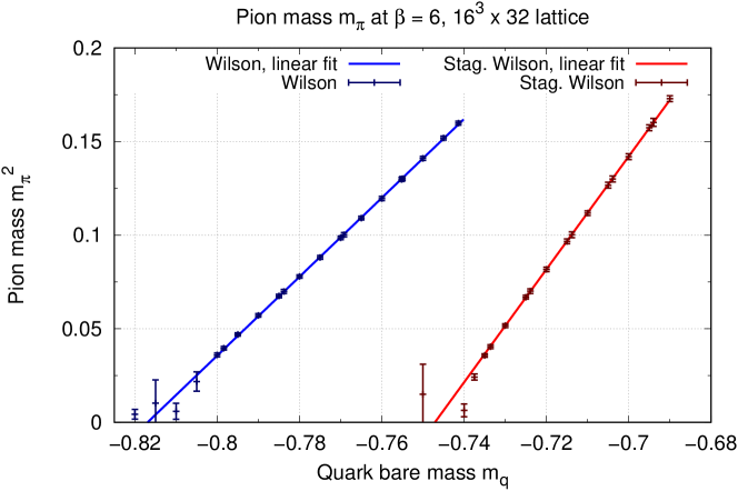
Figure 1: Squared pion mass $m_{\pi}^{2}$ as a function of the bare quark mass $m_{\mathsf{q}}$ with a linear fit through the data points with $0.05\leq m_{\pi}^{2}$.

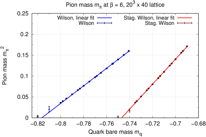
Figure 2: Squared pion mass $m_{\pi}^{2}$ as a function of the bare quark mass $m_{\mathsf{q}}$ with a linear fit through the data points with $0.05\leq m_{\pi}^{2}$.

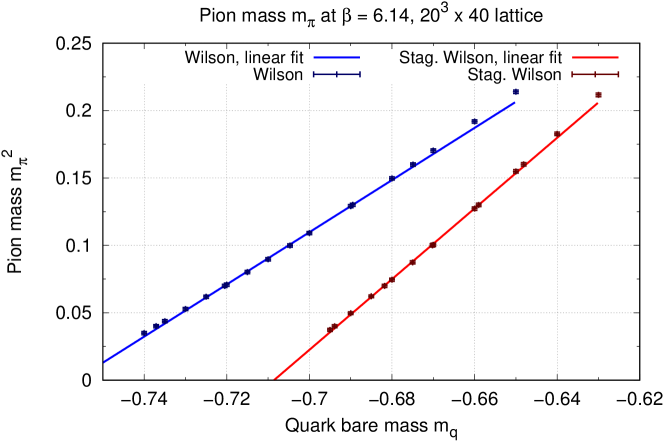
Figure 3: Squared pion mass $m_{\pi}^{2}$ as a function of the bare quark mass $m_{\mathsf{q}}$ with a linear fit through the data points with $0.05\leq m_{\pi}^{2}\leq 0.15$.

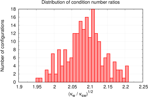
Figure 4: Distribution of $\sqrt{\kappa_{\mathsf{w}}/\kappa_{\mathsf{sw}}}$ for $m_{\pi}^{2}=0.10$ on the $20^{3}\times 40$ lattice at $\beta=6$.

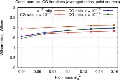
(a) Point sources

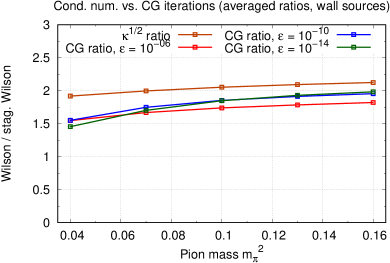
(b) Wall sources

Figure 5: Averages for the ratios of the number of iterations and $\sqrt{\kappa_{\mathsf{w}}/\kappa_{\mathsf{sw}}}$ as a function of the squared pion mass $m_{\pi}^{2}$ on a $16^{3}\times 32$ lattice at $\beta=6$.

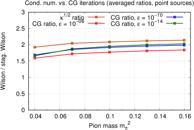
(a) Point sources

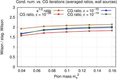
(b) Wall sources

Figure 6: Averages for the ratios of the number of iterations and $\sqrt{\kappa_{\mathsf{w}}/\kappa_{\mathsf{sw}}}$ as a function of the squared pion mass $m_{\pi}^{2}$ on a $20^{3}\times 40$ lattice at $\beta=6$.

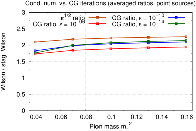
(a) Point sources

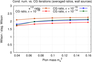
(b) Wall sources

Figure 7: Averages for the ratios of the number of iterations and $\sqrt{\kappa_{\mathsf{w}}/\kappa_{\mathsf{sw}}}$ as a function of the squared pion mass $m_{\pi}^{2}$ on a $20^{3}\times 40$ lattice at $\beta=6.136716$.

We did a numerical study with quenched QCD configurations on a $16^{3}\times 32$ lattice at $\beta=6$, a $20^{3}\times 40$ lattice at $\beta=6$ and a $20^{3}\times 40$ lattice at $\beta=6.136716$ with $200$ configurations each. The $20^{3}\times 40$ lattices are chosen in such a way to either keep the lattice spacing ($\beta=6$) or the physical volume ($\beta=6.136716$) fixed compared to the $16^{3}\times 32$ lattice. For the simulations we used the Chroma/QDP software package [87], which we extended by implementing staggered Wilson fermions.

While the use of preconditioning can speed up the use of Wilson fermions by roughly a factor of two and preconditioning is in principle also possible for staggered Wilson fermions, our study here deals with the unpreconditioned base case.

1 Results

In Figs. 1, 2 and 3, we find the squared pion mass $m_{\pi}^{2}$ as a function of the bare quark mass $m_{\mathsf{q}}$ for the different ensembles. The relation between the pion mass and bare quark mass for staggered Wilson fermions was previously also presented in Refs. [88, 4].

For the determination of the pion mass we follow the well-known standard procedures, see Ref. [17]. By inspecting the effective mass plot of the propagator, we fix a suitable fit range where the contributions of excited states is negligible and the signal-to-noise ratio is acceptable. We then do an uncorrelated fit of the pion propagator over the previously determined range using the function

$$p\left(n_{t}\right)=A\cosh\left(m_{\pi}\left[n_{t}-\frac{1}{2}N_{t}\right]\right)$$ (1)

by minimization of $\chi^{2}$, where $t=n_{t}a$ and the fit quality varies in the range $0.01\lesssim\chi/\textrm{d.o.f.}\lesssim 0.75$. Here the fit parameter $A$ is the amplitude, $m_{\pi}$ the pion mass and $N_{t}\in\left\{32,40\right\}$ is the extent of the corresponding lattice in temporal direction. The errors are combined statistical and systematic errors and are determined with the jackknife method [89, 90, 91], where we estimated the systematic error by varying the range of the fit.

In agreement with chiral perturbation theory, we find an approximately linear relationship between $m_{\pi}^{2}$ and $m_{\mathsf{q}}$. Moreover, the lowest achievable pion mass for Wilson and staggered Wilson fermions is comparable. We also note that the additive mass renormalization is smaller for staggered Wilson fermions compared to Wilson fermions. This could be a (somewhat weak) indicator for a computational advantage in the construction of overlap and domain wall fermions. Knowing the relation between the pion mass and the bare quark mass, for a given value of $m_{\pi}$ we can use the respective bare mass $m_{\mathsf{q}}$ for Wilson and staggered Wilson fermions. In the following, we fix five values of the pion mass, namely $m_{\pi}^{2}\in\left\{0.04,\,0.07,\,0.10,\,0.13,\,0.16\right\}$, as in general the efficiency is a function of the fixed physical parameter.

Using Chroma, we calculated the lowest and highest eigenvalue on each configurations to determine the conditions number $\kappa$ of $D^{\dagger}D$. With respect to Eq. (6), the ratio of the condition numbers is an important factor in judging the computational efficiency of staggered Wilson fermions. In Fig. 4, we give an example for the distribution of $\sqrt{\kappa_{\mathsf{w}}/\kappa_{\mathsf{sw}}}$ on one of our ensembles. As one can see, the square root of the ratio is of order $\mathcal{O}\left(2\right)$ and we conclude that the condition number of Wilson fermions in typically a factor $\mathcal{O}\left(4\right)$ higher compared to staggered Wilson fermions.

In Figs. 5, 6 and 7, we find the results for the ratio of the number of conjugate gradient iterations as given in Eq. (6). In the figures, we show both our theoretical estimate given by $\sqrt{\kappa_{\mathsf{w}}/\kappa_{\mathsf{sw}}}$ and the average measured ratios for the actual number of iterations needed as a function of the pion mass. We did this measurements for different values of the target residual $\varepsilon$ to check for a possible dependence. We also used two different kinds of sources, namely a point source and a wall source.

First we note that the choice of the source has no noticeable effect on the relative computational performance as the figures are nearly indistinguishable. Remarkably the dependence of the ratios on $m_{\pi}$ is also weak, although the number of conjugate gradient iterations grows strongly with decreasing pion masses. We can see that our rough theoretical estimate $\sqrt{\kappa_{\mathsf{w}}/\kappa_{\mathsf{sw}}}$ is a decent approximation for the actual measured ratios. Moreover, for smaller values of $\varepsilon$ the measured ratios become closer to our estimate as expected. In all cases we see that Wilson fermions need roughly $\mathcal{O}\left(2\right)$ more iterations in the application of the conjugate gradient method, which is in agreement with Ref. [71].

If we increase the physical volume in our simulation, i.e. when we compare the $16^{3}\times 32$ lattice at $\beta=6$ with the $20^{3}\times 40$ lattice at $\beta=6$, we find an improvement at small $m_{\pi}$, but otherwise almost unchanged results. If, on the other hand, we decrease the lattice spacing, i.e. when we compare the $16^{3}\times 32$ lattice at $\beta=6$ with the $20^{3}\times 40$ lattice at $\beta=6.136716$, we see a significant improvement in efficiency over the whole range of $m_{\pi}$. As the staggered Wilson Dirac operator is more sensitive to gauge fluctuations through its four-hop terms, we would expect that on smoother gauge configurations its convergence properties improve more compared to the Wilson Dirac operator.

2 Overall speedup

Combining the measured ratios from the previous discussion together with Eq. (10), the product in Eq. (4) takes the form

$$\frac{\mathrm{cost}_{\mathsf{W}}}{\mathrm{cost}_{\mathsf{SW}}}=\frac{\left(\textrm{\#iterations}\right)_{\mathsf{w}}}{\left(\textrm{\#iterations}\right)_{\mathsf{sw}}}\times\frac{\left(\textrm{cost mat-vec mult.}\right)_{\mathsf{w}}}{\left(\textrm{cost mat-vec mult.}\right)_{\mathsf{sw}}}\approx 2\times(2\text{--}3)=4\text{--}6.$$ (2)

This means that in our setting staggered Wilson fermions are a factor of $4\text{--}6$ more efficient than usual Wilson fermions for inverting the Dirac operator on a source. When computing the quark propagator, an additional factor of four should be included in Eq. (2) as for Wilson fermions one needs four times as many sources.

Before we move on with the discussion of arithmetic intensities, we add some critical remarks for the interpretation of the estimate given in Eq. (2). Our cost ratio is for the case of inverting the Dirac operator on a source and does not include the setup phase. For staggered Wilson fermions, one would typically prepare the averaged link products in the staggered Wilson term before applying the conjugate gradient method. The factor in Eq. (2) would therefore be a bit lower when taking the cost for this setup phase into account. Also, if one intends to do hadron spectroscopy with staggered Wilson fermions as described in Chapter 4, one has to take the additional number of sources needed into account, effectively reducing the computational advantage.

Moreover, when doing lattice field theoretical computations on high-performance computing clusters, communication over the network can become a bottleneck for the performance. As large-scale simulations of lattice quantum chromodynamics usually make use of a domain-decomposition approach and the staggered Wilson term connects each site with all the corners of the surrounding hypercube via four-hop terms, it is expected that the resulting network traffic will be significant. How severely this limits the performance of staggered Wilson fermions in large-scale simulations has yet to be seen. Until then, Eq. (2) should be taken as an estimate for the achievable performance gain on shared memory machines.

4 Arithmetic intensities

On modern computer architectures the performance of lattice field theoretical simulations is often not limited by the floating point throughput, but by limited memory bandwidth. A measure for the bandwidth requirements relative to the number of floating point operations (FLOPs) is the so called arithmetic intensity

$$I=\frac{\textrm{FLOPs}}{\textrm{Memory transactions in byte}}.$$ (1)

If for a given application this ratio is lower than what the respective hardware can provide, characterized by

$$I_{\mathsf{hw}}=\frac{\textrm{max.\,FLOPs\thinspace/\thinspace s}}{\textrm{max.\,memory bandwidth in byte\thinspace/\thinspace s}},$$ (2)

its performance is limited by the memory bandwidth. As a result, the computing cores spend some time with idling while waiting for the completion of memory access operations. On the other hand the performance of problems with high arithmetic intensity is limited by the floating point throughput of the hardware.

Simulations in the context of lattice quantum chromodynamics tend to have a rather low computational intensity, i.e. a relatively high number of memory transactions per floating point operation. If optimized properly, lattice codes can archive a high sustained performance on modern architectures. As the expected performance depends on the arithmetic intensity of the lattice fermion formulation, it is worth having a closer look.

In the following, we determine the arithmetic intensities for the application of several lattice Dirac operators in the setting of quantum chromodynamics, where we focus on the hopping-terms and exclude the trivial diagonal mass term. Within derivations we abbreviate FLOPs with $\mathtt{F}$. Before we begin, we note that for a complex addition we need $2\,\mathrm{\mathtt{F}}$ and for a complex multiplication we need $6\,\mathrm{\mathtt{F}}$. To multiply a complex $\mathrm{SU}\!\left(3\right)$ matrix with a complex three-component vector, we need $66\,\mathrm{\mathtt{F}}$. Regarding memory transactions, we assume single-precision floating point numbers, so-called floats, which are $32\,\mathrm{bit}$ or $4\,\mathrm{byte}$. Where convenient, we abbreviate floats by $\mathtt{fl}$. Depending on the application and hardware, in practice one might also use double-precision floating point numbers with $64\,\mathrm{bit}$ or $8\,\mathrm{byte}$, lowering the arithmetic intensity by a factor of two (see Ref. [92]). In some cases even mixed-precision is used, consisting of a combination of double-precision, single-precision and half-precision floating point numbers.

1 Wilson fermions

We begin with Wilson fermions as defined in Subsec. 6. We note that some fixed terms in the action can be precomputed, namely terms like $\mathbbm{1}\pm\gamma_{\mu}$, to save arithmetic operations. We also have to take into account that a competitive implementation of Wilson fermions employs the spin-projection trick [86], which reduces the number of spin components by a factor of two.

Floating point operations.

The spin projection takes $12\times 2\times 2\,\mathrm{\mathtt{F}}=96\,\mathrm{\mathtt{F}}$ (twelve operations $\times$ four directions $\times$ forward/backward) and for the link multiplications we need $66\times 2\times 4\times 2\,\mathrm{\mathtt{F}}=1056\,\mathrm{\mathtt{F}}$ (matrix-vector multiplication $\times$ two spin components $\times$ four directions $\times$ forward/backward). Accumulating the resulting vector takes $12\times 2\times 7\,\mathrm{\mathtt{F}}=168\,\mathrm{\mathtt{F}}$ (twelve components $\times$ cost per complex addition $\times$ adding eight vectors). In total we find that Wilson fermions take $1320\,\mathrm{\mathtt{F}/site}$. This result is in agreement with Refs. [93, 92, 94].

Memory access operations.

We need to read one spinor per direction, i.e. $12\times 2\times 4\times 2\,\mathrm{\mathtt{fl}}=192\,\mathrm{\mathtt{fl}}$ (twelve complex numbers per spinor $\times$ floats per complex number $\times$ four directions $\times$ forward/backward) and one $3\times 3$ gauge link per direction, i.e. $9\times 2\times 4\times 2\,\mathrm{\mathtt{fl}}=144\,\mathrm{\mathtt{fl}}$ (nine elements $\times$ floats per complex number $\times$ four directions $\times$ forward/backward). Writing the resulting spinor takes $12\times 2\,\mathrm{\mathtt{fl}}=24\,\mathrm{\mathtt{fl}}$. In total we find $360\,\mathrm{\mathtt{fl}/site}=1440\,\mathrm{byte/site}$ of memory access operations per lattice site. This result is also in agreement with Refs. [92, 94].

Arithmetic intensity.

We find

$$I_{\mathsf{w}}=\frac{1320\,\mathrm{FLOPs/site}}{1440\,\mathrm{byte/site}}\approx 0.92\,\mathrm{FLOPs/byte}$$ (3)

for the arithmetic intensity of Wilson fermions.

2 Staggered fermions

We are repeating the previous exercise now for usual staggered fermions, which we discussed in Subsec. 7.

Floating point operations.

For the link multiplications we have $66\times 4\times 2\,\mathrm{\mathtt{F}}=528\,\mathrm{\mathtt{F}}$ (matrix-vector multiplication $\times$ four directions $\times$ forward/backward). Accumulating the resulting vector takes $3\times 2\times 7\,\mathrm{\mathtt{F}}=42\,\mathrm{\mathtt{F}}$ (three color components $\times$ cost per complex addition $\times$ adding eight vectors). In total we find that usual staggered fermions need $570\,\mathrm{\mathtt{F}/site}$, which is in agreement with Ref. [95].

Memory access operations.

We read one spinor per direction, i.e. $3\times 2\times 4\times 2\,\mathrm{\mathtt{fl}}=48\,\mathrm{\mathtt{fl}}$ (three complex numbers per spinor $\times$ floats per complex number $\times$ four directions $\times$ forward/backward) as well as one gauge link per direction, i.e. $9\times 2\times 4\times 2\,\mathrm{\mathtt{fl}}=144\,\mathrm{\mathtt{fl}}$ (nine elements $\times$ floats per complex number $\times$ four directions $\times$ forward/backward). Writing the resulting spinor takes $3\times 2\,\mathrm{\mathtt{fl}}=6\,\mathrm{\mathtt{fl}}$. In total we have $198\,\mathrm{\mathtt{fl}/site}=792\,\mathrm{byte/site}$ of memory access operations per lattice site, which is also in agreement with Ref. [95].

Arithmetic intensity.

We find

$$I_{\mathsf{st}}=\frac{570\,\mathrm{FLOPs/site}}{792\,\mathrm{byte/site}}\approx 0.72\,\mathrm{FLOPs/byte}$$ (4)

for the arithmetic intensity of staggered fermions.

3 Staggered Wilson fermions

Compared to usual staggered fermions, staggered Wilson fermions have an additional term in the action. In the following, we only analyze the additional contributions from the staggered Wilson term and then add the respective counts to the numbers of usual staggered fermions.

Floating point operations.

Applying the $C$ operator takes $66\times 16\,\mathrm{\mathtt{F}}+3\times 2\times 15\,\mathrm{\mathtt{F}}=1146\,\mathrm{\mathtt{F}}$ (matrix-vector multiplication $\times$ number of hybercube corners $+$ three color components $\times$ cost per complex addition $\times$ adding sixteen vectors). Applying $\Gamma_{55}$ and $\eta_{5}$ takes $\left(3+6\right)\,\mathrm{\mathtt{F}}$. The $r\mathbbm{1}$ term can be combined with the diagonal mass term $m\mathbbm{1}$ and, thus, will be ignored as in the preceding calculations. Accumulating the resulting vector takes $3\times 2\times 1\,\mathrm{\mathtt{F}}=6\,\mathrm{\mathtt{F}}$ (three color components $\times$ cost per complex addition $\times$ adding two vectors). In total we find that staggered Wilson fermions take an additional $1161\,\mathrm{\mathtt{F}/site}$ compared to staggered fermions, i.e. $1731\,\mathrm{\mathtt{F}/site}$ in total. Note that when the diagonal $\left(m+r\right)\mathbbm{1}$ term is included we need additional $12\,\mathrm{\mathtt{F}}$, i.e. $1743\,\mathrm{\mathtt{F}/site}$ in agreement with Ref. [4].

Memory access operations.

We need to read one additional spinor per hypercube corner, i.e. $3\times 2\times 16\,\mathrm{\mathtt{fl}}=96\,\mathrm{\mathtt{fl}}$ (three complex numbers per spinor $\times$ floats per complex number $\times$ number of corners) and one gauge link per hypercube corner, i.e. $9\times 2\times 16\,\mathrm{\mathtt{fl}}=288\,\mathrm{\mathtt{fl}}$ (9 elements $\times$ floats per complex number $\times$ number of corners) for the $C$ operator. Write the resulting spinor takes $3\times 2\,\mathrm{\mathtt{fl}}=6\,\mathrm{\mathtt{fl}}$. This means that we have an additional $390\,\mathrm{\mathtt{fl}/site}=1560\,\mathrm{byte/site}$, i.e. in total we find $588\,\mathrm{\mathtt{fl}/site}=2352\,\mathrm{byte/site}$ for staggered Wilson fermions.

Arithmetic intensity.

We find

$$I_{\mathsf{stw}}=\frac{1731\,\mathrm{FLOPs/site}}{2352\,\mathrm{byte/site}}\approx 0.74\,\mathrm{FLOPs/byte}$$ (5)

for the arithmetic intensity of staggered Wilson fermions.

4 Summary

Formulation	Operations	I/O	Intensity	Source
Wilson	$1320$	$1440$	$0.92$	Here and Refs. [93, 92, 94]
Wilson + Clover	$1824$	$1728$	$1.06$	Ref. [94]
Staggered	$570$	$792$	$0.72$	Here and Ref. [95]
HISQ / asqtad	$1146$	$1560$	$0.73$	Ref. [94]
Staggered Wilson	$1731$	$2352$	$0.74$	Here and Ref. [4]

Table 1: Arithmetic intensities of several lattice Dirac operators. Operations are in units of FLOPs / site, I/O in bytes / site and Intensity in FLOPs / byte.

We summarize our findings in Table 1, where we added Wilson fermions with a clover term (see e.g. Ref. [16]) as well as HISQ [96] (highly improved staggered quarks) and asqtad [97] ($a$-squared tadpole improved) staggered fermions from the literature. We note that all staggered formulations have a very similar arithmetic intensity, while staggered Wilson fermions have slightly lower memory bandwidth requirements compared to the others. This means, that despite the large number of memory access operations per site needed for the application of the staggered Wilson Dirac operator, we do not expect a more severe memory bandwidth bottleneck.

One possibility to increase arithmetic intensities and to lower memory bandwidth requirements for all fermion formulations is to only load the first two rows of each $\mathrm{SU}\!\left(3\right)$ matrix and then reconstruct the last one by using unitarity. This lowers memory bandwidth requirements at the cost of additional FLOPs, thus increasing arithmetic intensity.

5 Conclusions

We estimated the speedup factor of staggered Wilson fermions to be $4\text{--}6$ compared to usual Wilson fermions for inverting the Dirac matrix on a source. However, it is important to keep the critical remarks from Subsec. 2 in mind when interpreting this result.

To allow for an easier comparison, we discussed here the case of kernel operators which are both unpreconditioned and unimproved. While for Wilson fermions many preconditioned and improvement variants are known and in use, there are many possibilities to further improve the computational efficiency of staggered Wilson fermions as well. One could replace the usual staggered part of staggered Wilson fermions by the HISQ action to reduce $\mathcal{O}\left(a^{2}\right)$ effects and use link smearing. While a certain form of a clover term for $\mathcal{O}\left(a\right)$ improvement was studied in Ref. [82], there is also the possibility for the introduction of other clover terms.

Finally, comparing the arithmetic intensities of the different fermion formulations in Sec. 4, we note that the memory bandwidth requirements of staggered Wilson fermions are slightly lower compared to other staggered formulations. As memory bandwidth is usually a limiting factor for the performance of lattice codes, this is important in the context of writing highly optimized implementations of the Dirac operator.

Chapter 4 Pseudoscalar meson spectrum

One of the traditional applications of lattice gauge theory is hadron spectroscopy. In this setting not only computational efficiency, but also the usability of the formalism is important. To show the feasibility of doing spectroscopy with staggered Wilson fermions, in this chapter we discuss the case of pions, i.e. pseudoscalar mesons.

For usual staggered fermions the four tastes give rise to sixteen pions. In the following we study the pion spectrum of staggered fermions when turning Adams’ two-flavor staggered Wilson term on. The effect of this term is that two of the four tastes acquire a mass of $\mathcal{O}\left(a^{-1}\right)$ and become heavy. As a result, we find that eight of the pions become heavy as well, while the other eight remain light. In the physical light part of the spectrum we find the degenerate two-flavor pion-triplet and the flavor-singlet $\eta$ meson with each coming in two copies. The $\eta$ meson remains light as we omit the disconnected piece of the propagator in our study. Some of the results discussed here were previously presented in Refs. [9, 10].

1 Introduction

From a practitioner’s point of view, the usability of a lattice formulation is important. To show that staggered Wilson fermions are not at a disadvantage compared to other fermion formulations, we illustrate spectroscopy calculations as one of the traditional applications of lattice quantum chromodynamics (QCD). Like for other staggered formulations, spin and flavor degrees of freedom are distributed over different lattice sites. We will see, that one can easily adapt the spectroscopy methods and operators of usual staggered fermions to the two flavor case, as we are going to illustrate for the case of pions.

In this work we deal with Adams’ original two flavor proposal [44, 45], where the action reads

$$S_{\mathsf{sw}}=\bar{\chi}\left(D_{\mathsf{st}}+m_{\mathsf{q}}+W_{\mathsf{st}}\right)\chi,\qquad W_{\mathsf{st}}=\frac{r}{a}\left(\mathbbm{1}-\Gamma_{55}\Gamma_{5}\right)$$ (1)

and $D_{\mathsf{st}}=\eta_{\mu}\nabla_{\mu}$ refers to the staggered Dirac operator, $m_{\mathsf{q}}$ to the bare quark mass, $W_{\mathsf{st}}$ to the staggered Wilson term as defined in Sec. 4, $a$ to the lattice spacing and $r>0$ is the equivalent of the Wilson parameter. Here and in the following, the $\xi_{\mu}$ matrices refer to a representation of the Dirac algebra in flavor space and in figures we use the shorthand notation $\xi_{\mu\nu}\equiv\xi_{\mu}\xi_{\nu}$.

This chapter is organized as follows. In Sec. 2, we discuss pseudoscalar mesons in the framework of usual staggered fermions and generalize the known methods to the case of staggered Wilson fermions. In Sec. 3, we discuss our numerical results and compare them to our theoretical predictions. Finally, in Sec. 4 we summarize our results and end with some concluding remarks.

2 Pseudoscalar mesons

For usual staggered fermions, the meson and baryon rest-frame operators are known [98] and we can adapt these operators to the two-flavor staggered Wilson case. However, as two of the four tastes become heavy after the introduction of the staggered Wilson term, the physical interpretation of these operators change. In the following, we will discuss the case of pseudoscalar mesons both from a theoretical and numerical point of view. We first begin with reviewing the case of usual staggered fermions, before we move on to staggered Wilson fermions.

Staggered fermions have four (quark) tastes, giving rise to sixteen pseudoscalar mesons. They have a spin$\,\otimes\,$flavor structure $\gamma_{5}\otimes\xi_{\mathsf{F}}$ with

$$\xi_{\mathsf{F}}\in\left\{\mathbbm{1},\,\xi_{5},\,\xi_{\mu},\,\xi_{\mu}\xi_{5},\,\xi_{\mu}\xi_{\nu}\right\}.$$ (1)

On the lattice the states fall into eight irreducible representations of the lattice timeslice group [98], namely

$$\xi_{4}\xi_{5},\,\xi_{5},\,\xi_{i}\xi_{5},\,\xi_{i}\xi_{j},\,\xi_{i},\,\xi_{i}\xi_{4},\,\mathbbm{1},\,\xi_{4}.$$ (2)

Here the $\gamma_{5}\otimes\xi_{5}$ state corresponds to the Goldstone pion for the axial symmetry at vanishing $m_{\mathsf{q}}$. While for staggered fermions the continuum $\mathrm{SU}\!\left(4\right)$ flavor symmetry is broken down to a discrete subgroup, by doing a joint expansion in $m_{\mathsf{q}}$ and $a^{2}$ one can show that the pion masses are $\mathrm{SO}\!\left(4\right)$ symmetric up to leading discretization errors, see Ref. [99].

Within these representations we find two distinct types of states: while some states propagate with a $\left(-1\right)^{t}$-factor in time, others do not. The timeslice operators, in general, excite both these kinds of states, i.e. if an operator couples to $\gamma_{\mathsf{S}}\otimes\xi_{\mathsf{F}}$, then it also couples to $\gamma_{4}\gamma_{5}\gamma_{\mathsf{S}}\otimes\xi_{4}\xi_{5}\xi_{\mathsf{F}}$. In the case of pseudoscalar mesons we have $\gamma_{\mathsf{S}}\in\left\{\gamma_{5},\,\gamma_{4}\gamma_{5}\right\}$. The fact that we excite two states simultaneously does not pose a problem as both states can be easily separated by their distinct time-dependence. We can parametrize the time-time correlation function by

$$f_{R_{\pm},m_{\pm}}\left(n_{t}\right)=R_{+}\cosh\left[m_{+}\left(n_{t}-\frac{1}{2}N_{t}\right)\right]+\left(-1\right)^{n_{t}}R_{-}\cosh\left[m_{-}\left(n_{t}-\frac{1}{2}N_{t}\right)\right],$$ (3)

where $t=n_{t}a$ and we assume that one-particle states are dominant [98]. Here $R_{\pm}$ and $m_{\pm}$ are the amplitudes and masses of both respective states and $N_{t}$ refers to the number of timeslices of the lattice.

After the introduction of the staggered Wilson term, two tastes become heavy and $\xi_{\mathsf{F}}$ can be thought of having the structure

$$\xi_{\mathsf{F}}\cong\left[\begin{array}[]{cc}\textrm{light\thinspace+\thinspace light}&\textrm{light\thinspace+\thinspace heavy}\\ \textrm{heavy\thinspace+\thinspace light}&\textrm{heavy\thinspace+\thinspace heavy}\end{array}\right].$$ (4)

In the continuum limit, the heavy quark content decouples and the “light + light” part of $\xi_{\mathsf{F}}$ determines the physical interpretation. To give an example, consider

$$\xi_{\mathsf{F}}=\xi_{1}\xi_{2}=\left(\begin{array}[]{cc}\textrm{i}\sigma_{3}\\ &\textrm{i}\sigma_{3}\end{array}\right).$$ (5)

The physically relevant part is $\textrm{i}\sigma_{3}$, hence $-\textrm{i}\bar{\chi}\left(\gamma_{5}\otimes\xi_{3}\xi_{4}\right)\chi$ corresponds to a $\pi^{0}$ operator, see also Ref. [9].

Flavor matrix $\xi_{\mathsf{F}}$	Composition	Particles
$\xi_{k}\xi_{4}$	$\overline{q}\sigma_{k}q$	$\pi$ triplet
$\xi_{i}\xi_{j}$
$\xi_{5}$	$\overline{q}q$	$\eta$ singlet
$\mathbbm{1}$

Table 1: Pseudoscalar meson spectrum for staggered Wilson fermions ($i$, $j$ and $k$ mutually distinct).

After analyzing all states, one finds that for $\xi_{\mathsf{F}}\in\left\{\xi_{4}\xi_{5},\,\xi_{i}\xi_{5},\,\xi_{i},\,\xi_{4}\right\}$ there are only contributions from heavy tastes. For the states with $\xi_{\mathsf{F}}\in\left\{\xi_{5},\,\xi_{i}\xi_{j},\,\xi_{i}\xi_{4},\,\mathbbm{1}\right\}$, we find a mixture of purely light and purely heavy quark content, where the heavy contributions decouple in the continuum limit. In total we find that from the sixteen pseudoscalar mesons for usual staggered fermions only eight remain light in the presence of the staggered Wilson term. Among these eight light pions we find two copies of the two-flavor pion triplet, which only differ by their heavy quark content. We note that the pion triplet for staggered Wilson fermions is degenerated as discussed in Ref. [69]. In addition we find two copies of the flavor-singlet $\eta$ meson. These light states and their physical interpretation are summarized in Table 1, where $q=\left(q_{1},q_{2}\right)^{\intercal}$ denotes the two physical tastes.

3 Numerical results

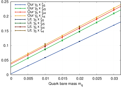
(a) Part I

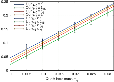
(b) Part II

Figure 1: Comparison between the pseudoscalar meson masses $m^{2}\left(m_{\mathsf{q}}\right)$ at $r=0$ in our study with the literature values from Ref. [100].

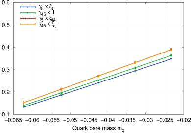
(a) Physical pseudoscalar mesons

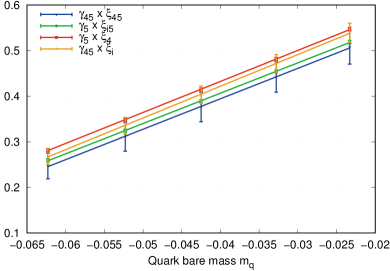
(b) Heavy pseudoscalar mesons

Figure 2: Pseudoscalar meson masses $m^{2}\left(m_{\mathsf{q}}\right)$ at $r=0.1$.

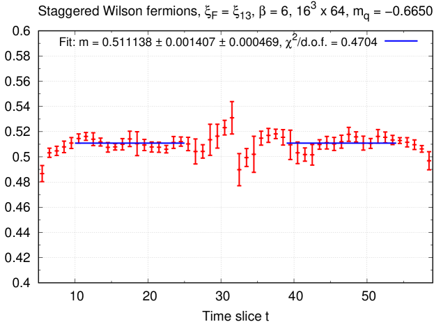
Figure 3: Effective mass plot $m_{\mathsf{eff}}\left(t\right)$ together with the fitted mass $m$ and its statistical and systematic error at $r=1$ for the light pseudoscalar meson with $\xi_{\mathsf{F}}=\xi_{1}\xi_{3}$.

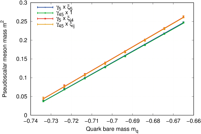
Figure 4: Pseudoscalar meson spectrum for two-flavor staggered Wilson fermions ($r=1$).

To illustrate the practicality of spectrum calculations with staggered Wilson fermions and to verify the results from the previous section, we implemented staggered Wilson fermions in the Chroma/QDP software package [87]. The software suite comes with an application for spectrum calculations with staggered fermions. For the pseudoscalar mesons operators we used the operators that are already implemented and which match the ones used in Ref. [100].

Our quenched QCD study was carried out using $200$ gauge configurations at a coupling of $\beta=6$ on a $16^{3}\times 64$ lattice, where we fixed the configurations to Coulomb gauge. On each configuration we evaluated eight staggered wall sources, i.e. wall sources where within the wall there is a one in a single corner of each of the spatial cubes and zero everywhere else. By combining them appropriately, we can project onto the irreducible representations of the timeslice group [100]. To extract the pseudoscalar meson masses, we essentially follow the method described in Subsec. 1. To compute effective masses, we can do a minimization of the form $\min_{R_{\pm},m_{\pm}}\left\|F_{R_{\pm},m_{\pm}}\right\|$ with

$$F_{R_{\pm},m_{\pm}}=\left(\begin{array}[]{c}f_{R_{\pm},m_{\pm}}\left(n_{t}+0\right)-p\left(n_{t}+0\right)\\ f_{R_{\pm},m_{\pm}}\left(n_{t}+1\right)-p\left(n_{t}+1\right)\\ f_{R_{\pm},m_{\pm}}\left(n_{t}+2\right)-p\left(n_{t}+2\right)\\ f_{R_{\pm},m_{\pm}}\left(n_{t}+3\right)-p\left(n_{t}+3\right)\end{array}\right),$$ (1)

where $f_{R_{\pm},m_{\pm}}\left(n_{t}\right)$ refers to the fit function defined in Eq. (3) and $p\left(n_{t}\right)$ to the corresponding time-time correlation function. In the final four parameter fit of Eq. (3) we fixed the fit range from $n_{1}=10$ to $n_{2}=25$ together with the mirrored range $N_{t}-n_{2}$ to $N_{t}-n_{1}$ for all pions, where $N_{t}=64$ is the extent of the lattice in temporal direction. Correlations are neglected in the $\chi^{2}$-fit. The errors are estimated in the same way as described in Subsec. 1.

As a check of the correctness of our method and fitting procedure, we reproduced the known results from Ref. [100] (cf. Ref. [101]) for the case of usual staggered fermions. By setting the staggered Wilson parameter to $r=0$ in Eq. (1) for this test, we can calculate the pseudoscalar meson spectrum and find an excellent match with the literature values, see Fig. 1. In this figure and the following mass plots, for every pseudoscalar meson mass $m$ we add a linear fit of the form $m^{2}=c_{1}m_{\mathsf{q}}+c_{2}$.

As the negative flavor-chirality species acquire a mass of $\mathcal{O}\left(r/a\right)$ in the presence of the staggered Wilson term, we can use $r$ to control the masses of the heavy pseudoscalar mesons. We can then consider staggered Wilson fermions with a small $r$ to observe how a mass splitting between the light and heavy pions forms. In Fig. 2, we can find the spectrum for $r=0.1$, where in the left part of the figure we can find all light pions and in the right part the heavy pions. Using the same scale for the vertical axes, one can see how the heavy pseudoscalar mesons are systematically shifted upwards due to contributions from heavy tastes.

Moving on to staggered Wilson fermions with $r=1$, the initially small mass gap between the light and heavy pion states becomes large. In Fig. 3, we can see a representative effective mass plot for the state with $\xi_{\mathsf{F}}=\xi_{1}\xi_{3}$, which remains light after the introduction of the staggered Wilson term in agreement with Table 1 and the discussion in Sec. 2. On the other hand, the heavy states now have a mass of $m=\mathcal{O}\left(a^{-1}\right)$. As the condition $am\ll 1$ is violated, one would not expect to be able to reliably describe these states on our lattices.

Finally, focusing on the physical (light) part of the pseudoscalar mesons, we find the resulting spectrum of pseudoscalar mesons for two-flavor staggered Wilson fermions in Fig. 4. As predicted by chiral perturbation theory, we find that the squared pseudoscalar meson masses $m^{2}$ are approximately linear in the bare quark mass $m_{\mathsf{q}}$. Referring to Table 1, in the continuum limit the pairs $\left\{\xi_{5},\,\mathbbm{1}\right\}$ and $\left\{\xi_{k}\xi_{4},\,\xi_{i}\xi_{j}\right\}$ are expected to be degenerated as the heavy quark content decouples. In the present setting with a finite lattice spacing these degeneracies only hold approximately, but already describe the observed spectrum well. Moreover, we observe that both pairs separate well. We note that in our calculations the flavor-singlet $\eta$ remains light due to the omission of the disconnected piece of the propagator.

4 Conclusions

The aim of this study was to demonstrate the feasibility of spectrum calculations with Adams’ two-flavor staggered Wilson fermions. To this end we determined how the pseudoscalar spectrum can be computed and changes with the presence of the staggered Wilson term.

In the physical part of the spectrum we find two copies for both the degenerate two-flavor pion-triplet as well as the flavor-singlet $\eta$ meson. We conclude that two-flavor staggered Wilson fermions work as expected for studying pseudoscalar mesons. In future work one can investigate spectroscopy of other hadrons, in particular also baryons, where our approach is expected to generalize.

Chapter 5 Staggered overlap fermions

Chiral symmetry plays an important role in understanding the low-energy regime of quantum chromodynamics, in particular hadron phenomenology. As discussed in Subsec. 4, the Nielsen-Ninomiya theorem [31, 30, 32, 33] complicates the implementation of chiral symmetry on the lattice. With the overlap construction [102, 103, 104, 105, 106, 107, 108] this problem could eventually be overcome and one can formulate a lattice Dirac operator with exact chiral symmetry [109, 110, 111]. While the overlap formalism has many attractive theoretical properties, its practical applications are limited due to the fact that overlap fermions typically require a factor of $\mathcal{O}\left(10\text{--}100\right)$ more computational resources compared to Wilson fermions.

The prospect of a staggered overlap operator becomes interesting as it can potentially bring down the enormous costs of lattice theoretical simulations in which chiral symmetry is of importance. Usual staggered fermions do not define a suitable kernel operator for the overlap formalism due to the fact that the staggered equivalent of $\gamma_{5}$, namely the $\Gamma_{5}\cong\gamma_{5}\otimes\mathbbm{1}+\mathcal{O}\left(a^{2}\right)$ operator, does not square to the identity, i.e. $\Gamma_{5}^{2}\neq\mathbbm{1}$. As Adams pointed out in Refs. [44, 45, 112], this problem can be solved with the help of the staggered Wilson construction, where on the physical species $\Gamma_{55}$ can be used for $\gamma_{5}$. As $\Gamma_{55}^{2}=\mathbbm{1}$ holds exactly, this allows the construction of staggered variants of overlap and domain wall fermions.

In this chapter, we discuss Neuberger’s overlap fermions in Sec. 1 and then introduce Adams’ staggered overlap construction in Sec. 2. This is followed by a review of the index theorem in Sec. 3. In Sec. 4, we verify that the continuum limit of the index and axial anomaly for the staggered overlap Dirac operator is correctly reproduced. This is meant as a first step to place staggered overlap fermions on solid theoretical foundations. Our analytical work was first presented in Ref. [3], where later a more comprehensive discussion was given by Har in Ref. [11].

1 Neuberger’s overlap fermions

We begin by discussing the Ginsparg-Wilson relation in Subsec. 1 and Neuberger’s overlap construction in Subsec. 2, following the outline of Ref. [16].

1 The Ginsparg-Wilson relation

The Nielsen-Ninomiya theorem prevents a straight-forward implementation of chiral symmetry on the lattice of the form $\left\{D,\gamma_{5}\right\}=0$. To circumvent this problem, Ginsparg and Wilson proposed in Ref. [109] to replace the continuum expression by

$$\left\{D,\gamma_{5}\right\}=aD\gamma_{5}D.$$ (1)

For this so-called Ginsparg-Wilson relation in Eq. (1) we see that the anticommutator is not vanishing on the lattice, but is instead an order $\mathcal{O}\left(a\right)$ term, eventually shrinking to zero in the continuum limit. A remarkable observation is now that, while the continuum form of chiral symmetry is recovered in the $a\to 0$ limit, even at a finite lattice spacing a Dirac operator $D$ satisfying Eq. (1) has an exact chiral symmetry. However, for a long time no solution to the Ginsparg-Wilson relation was known and the possibility of finding a closed solution in the interacting case was doubted. Only much later solutions were explicitly constructed, namely overlap fermions [108] and fixed points fermions [113].

Assuming that a Dirac operator $D$ satisfies the Ginsparg-Wilson relation, one can define an infinitesimal chiral transformation of the form

$$\delta\overline{\Psi}=\overline{\Psi}\gamma_{5},\qquad\delta\Psi=\gamma_{5}\left(\mathbbm{1}-aD\right)\Psi,$$ (2)

where the corresponding finite transformation takes the form

$$\overline{\Psi}\to\overline{\Psi}e^{\textrm{i}\alpha\gamma_{5}},\qquad\Psi\to e^{\textrm{i}\alpha\gamma_{5}\left(\mathbbm{1}-aD\right)}\Psi$$ (3)

with $\alpha\in\mathbb{R}$ being a continuous parameter. We note that these transformations can also be written in a symmetric form, where both $\overline{\Psi}$ and $\Psi$ transform with a factor of $\gamma_{5}\left(\mathbbm{1}-aD/2\right)$. One can easily verify the invariance of the action $S=\overline{\Psi}D\Psi$ under these chiral transformations, where in the $a\to 0$ limit the continuum expressions are reproduced.

Now let us impose that $D$ is also $\gamma_{5}$ Hermitian, i.e. $D^{\dagger}=\gamma_{5}D\gamma_{5}$. This ensures that complex eigenvalues come in conjugated pairs and $\det D\in\mathbb{R}$. Another important consequence is that for an eigenvector $v_{\lambda}$ of $D$, corresponding to the eigenvalue $\lambda$, one can verify that

$$\left\langle v_{\lambda},\gamma_{5}v_{\lambda}\right\rangle=0,$$ (4)

unless $\lambda\in\mathbb{R}$. Here $\left\langle v,w\right\rangle=v^{\dagger}w$ denotes the usual inner product of $\mathbb{C}^{n}$. This means that only eigenmodes with real eigenvalues can have definite chirality.

Going back to the Ginsparg-Wilson relation in Eq. (1), we can see that by multiplying with $\gamma_{5}$ from either the left or the right side and using $\gamma_{5}$ Hermiticity, one finds that

$$aD^{\dagger}D=D^{\dagger}+D=D+D^{\dagger}=aDD^{\dagger},$$ (5)

so $D$ is a normal operator satisfying $\left[D^{\dagger},D\right]=0$. As a consequence one finds

$$\lambda+\lambda^{\star}=a\lambda\lambda^{\star}$$ (6)

for the eigenvalues. Writing the eigenvalues explicitly with real and imaginary part, this equation takes the form

$$\left(\operatorname{Re}\lambda-\frac{1}{a}\right)^{2}+\left(\operatorname{Im}\lambda\right)^{2}=\frac{1}{a^{2}}$$ (7)

and one can see that they lie on a circle in the complex plane, commonly referred to as the Ginsparg-Wilson circle.

As the Ginsparg-Wilson circle is going through the origin, $D$ can have exact zero modes. If $v_{0}$ denotes such a zero mode, one can verify that

$$Dv_{0}=\gamma_{5}Dv_{0}=D\gamma_{5}v_{0}=0.$$ (8)

Thus on the eigenspace for the eigenvalue zero the Dirac operator $D$ and the chirality operator $\gamma_{5}$ commute. One can now choose the eigenvectors so that they are simultaneously eigenmodes of both $D$ and $\gamma_{5}$. We can then write

$$\gamma_{5}v_{0}=\pm v_{0},$$ (9)

where the eigenvalues are $\pm 1$ due to $\gamma_{5}^{2}=\mathbbm{1}$. This means that the zero modes of $D$ have definite chirality. If we find a plus sign in Eq. (9), we say that $v_{0}$ has positive chirality or call it right-handed, otherwise we say that $v_{0}$ has negative chirality or call it left-handed.

2 The overlap operator

While for a long time the search for an explicit solution to the Ginsparg-Wilson relation was not successful, eventually a solution in the form of the overlap operator was found. The overlap formalism was developed over the course of several papers [102, 103, 104, 105, 106, 107, 108] and finally brought into its present day form by Neuberger [106, 107, 108]. The Dirac operator reads

$$D_{\mathsf{ov}}=\frac{1}{a}\left(\mathbbm{1}+A\left[A^{\dagger}A\right]^{-\frac{1}{2}}\right)=\frac{1}{a}\left(\mathbbm{1}+\gamma_{5}H/\sqrt{H^{2}}\right)=\frac{1}{a}\left(\mathbbm{1}+\gamma_{5}\operatorname{sign}H\right)$$ (10)

with kernel operator $A=D_{\mathsf{w}}\left(-M_{0}\right)$, Hermitian operator $H=\gamma_{5}D_{\mathsf{w}}\left(-M_{0}\right)$ and negative mass parameter $M_{0}$. In the free-field case valid choices are in the range $M_{0}\in\left(0,2r\right)$, where $r$ denotes the Wilson parameter, to give rise to a one flavor theory. In some contexts there is an additional rescaling of $D_{\mathsf{ov}}$ by some factor $\rho$, see our discussion in Chapter 7. In principle one can replace the Wilson Dirac operator $D_{\mathsf{w}}$ also by some other suitable $\gamma_{5}$ Hermitian kernel operator. Using the fact that $\operatorname{sign}^{2}H=\mathbbm{1}$, one can easily verify that the overlap Dirac operator satisfies the Ginsparg-Wilson relation in Eq. (1).

The overlap Dirac operator in Eq. (10) is not ultralocal due to the presence of the $1/\sqrt{H^{2}}$ term. Here we call a lattice Dirac operator $D$ ultralocal if $\exists l\geq 0$ so that $\left|D\left(x,\alpha,a;y,\beta,b\right)\right|=0$ for $\left\|x-y\right\|_{1}>l$, where $D\left(x,\alpha,a;y,\beta,b\right)$ denotes the matrix element of $D$ connecting the space-time coordinates $x$ and $y$ with respective spin components $\alpha$, $\beta$ and color components $a$, $b$. Under some general assumptions this lack of ultralocality holds in fact for all solutions of the Ginsparg-Wilson relation [114]. However, locality of $D_{\mathsf{ov}}$ could be established in Ref. [115] in the form of

$$\left|D_{\mathsf{ov}}\left(x,\alpha,a;y,\beta,b\right)\right|\leq\lambda\,e^{-\gamma/a\cdot\left\|x-y\right\|_{1}}.$$ (11)

Here $\lambda\geq 0$ and $\gamma>0$ are constants independent of the gauge field. As a result, the decay constant $a/\gamma$ vanishes in the continuum limit $a\to 0$ and a local quantum field theory is recovered.

The presence of the $\operatorname{sign}$-function in Eq. (10) makes the application of the overlap Dirac operator computational expensive. As mentioned earlier, one typically needs an factor of $\mathcal{O}\left(10\text{--}100\right)$ more computational resources compared to Wilson fermions. As a consequence the use of overlap fermions is limited in practical applications and a lot of past work deals with the efficient numerical treatment of the $\operatorname{sign}$-function, see e.g. Refs. [116, 117, 118, 119, 120].

2 Staggered overlap fermions

When applying the overlap construction to the staggered Dirac operator, one encounters some severe problems. For the resulting operator the remnant chiral symmetry is lost, the Ginsparg-Wilson relation does not hold and exact zero modes are absent [45].

These problems can be traced back to the fact that the overlap construction relies on the property $\gamma_{5}^{2}=\mathbbm{1}$, while this does not hold for the staggered equivalent $\Gamma_{5}\cong\gamma_{5}\otimes\mathbbm{1}+\mathcal{O}\left(a^{2}\right)$. The eigenvalues of $\gamma_{5}$ are $\pm 1$, while the eigenvalues of $\Gamma_{5}$ are distributed throughout the interval $\left[-1,1\right]$ and include zero as can be seen from the momentum representation $\prod_{\mu}\cos^{2}p_{\mu}$ of $\Gamma_{5}^{2}$ in the free-field case [112]. Finally, we note that the operator $\Gamma_{5}D_{\mathsf{st}}$, unlike its Wilson equivalent $\gamma_{5}D_{\mathsf{w}}$, is even lacking Hermiticity [112]. For these reasons the overlap construction with a usual staggered kernel does not give rise to a proper lattice fermion formulation.

All these problems could be eventually overcome by Adams’ construction introduced in Refs. [44, 45, 112]. The idea is that, after the introduction of the staggered Wilson term, one can use the $\Gamma_{55}$ operator instead of $\Gamma_{5}$. Although $\Gamma_{55}$ has a spin$\,\otimes\,$flavor interpretation [42] of $\Gamma_{55}\cong\gamma_{5}\otimes\xi_{5}$, the staggered Wilson term projects out the negative flavor-chirality species and we find $\Gamma_{55}\cong\Gamma_{5}+\mathcal{O}\left(a^{2}\right)$ on the physical species. Furthermore, $\Gamma_{55}^{2}=\mathbbm{1}$ holds exactly and $H_{\mathsf{sw}}=\Gamma_{55}D_{\mathsf{sw}}$ defines a Hermitian operator.

As a consequence, one can apply the overlap construction to the staggered Wilson kernel with the help of a simple replacement rule given by

$$D_{\mathsf{w}}\to D_{\mathsf{sw}},\qquad\gamma_{5}\to\Gamma_{55}$$ (1)

as derived in Refs. [44, 45, 112]. Explicitly, the staggered overlap operator $D_{\mathsf{so}}$ reads

$$D_{\mathsf{so}}=\frac{1}{a}\left(\mathbbm{1}+A\left[A^{\dagger}A\right]^{-\frac{1}{2}}\right)=\frac{1}{a}\left(\mathbbm{1}+\Gamma_{55}\frac{H_{\mathsf{sw}}}{\sqrt{H_{\mathsf{sw}}^{2}}}\right)=\frac{1}{a}\left(\mathbbm{1}+\Gamma_{55}\operatorname{sign}H_{\mathsf{sw}}\right)$$ (2)

with kernel operator $A=D_{\mathsf{sw}}\left(-M_{0}\right)$, Hermitian operator $H=\Gamma_{55}D_{\mathsf{sw}}\left(-M_{0}\right)$ and negative mass parameter $M_{0}$ within the range $M_{0}\in\left(0,2r\right)$ in the free-field case. We find that the action $S_{\mathsf{so}}=\overline{\chi}D_{\mathsf{so}}\chi$ is invariant under the infinitesimal transformation

$$\delta\overline{\chi}=\overline{\chi}\,\Gamma_{55},\qquad\delta\chi=\Gamma_{55}\left(\mathbbm{1}-aD_{\mathsf{so}}\right)\chi,$$ (3)

cf. Eq. (2) for the usual overlap operator. Furthermore, the staggered overlap operator satisfies the Ginsparg-Wilson relation

$$\left\{\Gamma_{55},D_{\mathsf{so}}\right\}=\frac{a}{r}D_{\mathsf{so}}\Gamma_{55}D_{\mathsf{so}}.$$ (4)

As in four space-time dimensions $D_{\mathsf{sw}}$ describes two tastes, the staggered overlap operator $D_{\mathsf{so}}$ represents two degenerate chiral fermion species on the lattice, which can be used to describe e.g. the up and down quark.

3 The index theorem and the axial anomaly

With respect to the topological aspects we are discussing throughout this thesis, let us introduce some important concepts from topology. If $n_{\mp}$ denote the number of left-handed and right-handed zero modes, then we define the integer-valued $\operatorname{index}$ of the Dirac operator $D$ as

$$\operatorname{index}D=n_{-}-n_{+}.$$ (1)

In the $d$-dimensional ($d$ even) continuum setting of quantum chromodynamics, the famous Atiyah-Singer index theorem [121, 122, 123, 124] states that

$$n_{-}-n_{+}=\left(-1\right)^{d/2}Q_{\mathsf{cont}},$$ (2)

where $Q_{\mathsf{cont}}$ is the so-called topological charge given by

$$Q_{\mathsf{cont}}=\intop\mathrm{d}^{4}x\,q_{\mathsf{cont}}\left(x\right),\qquad q_{\mathsf{cont}}\left(x\right)=\frac{1}{32\pi^{2}}\varepsilon_{\mu\nu\rho\sigma}\operatorname{tr}\left[F_{\mu\nu}\left(x\right)F_{\rho\sigma}\left(x\right)\right]$$ (3)

and $F_{\mu\nu}\left(x\right)$ is the corresponding field strength tensor. The index theorem in Eq. (2) is remarkable given the fact that the right hand side appears to be a continuous function of the gauge field, while the left hand side is an integer number. On the lattice one can formulate a similar index theorem [110], which reads

$$n_{-}-n_{+}=\left(-1\right)^{d/2}Q$$ (4)

with

$$Q=a^{4}\sum_{x\in\Lambda}q\left(x\right),\qquad q\left(x\right)=\frac{1}{2a^{3}}\operatorname{tr}\left[\gamma_{5}D\left(x,x\right)\right].$$ (5)

We note that in practice one never finds both $n_{-}$ and $n_{+}$ to be non-vanishing at the same time on thermalized configurations, i.e. one finds either $n_{-}=\left(-1\right)^{d/2}Q$ or $n_{+}=\left(-1\right)^{1+d/2}Q$. Moreover, in two dimensions one can show the Vanishing Theorem [125, 126, 127]. That is, one can prove that if $Q\neq 0$, then either $n_{-}$ or $n_{+}$ necessarily vanishes.

While a chiral flavor-singlet rotation is a symmetry of the action for a Dirac operator satisfying the Ginsparg-Wilson relation, the path integral itself is not invariant due to the nontrivial transformation of the integration measure [110, 111], cf. Refs. [128, 129, 130, 131, 132] for the continuum case. This so-called axial anomaly results in an anomalous continuity equation for the singlet axial vector current. The presence of the axial anomaly implies that there is no flavor-singlet Goldstone particle and explains why the $\eta$-meson is significantly heavier than the pions assuming an approximate chiral symmetry for two flavors, see e.g. Ref. [16]. In the three flavor case the Witten-Veneziano formula [133, 134, 135, 136, 137, 138, 139, 140] connects the mass of the $\eta^{\prime}$-meson to the topological susceptibility $\chi_{\mathsf{top}}=\left\langle Q^{2}\right\rangle/V$, where $V$ is the space-time volume.

4 Continuum limit of the index and axial anomaly

Massless overlap fermions have exact zero modes with definite chirality and one can define an index for the overlap Dirac operator as discussed in Subsec. 3. Overlap fermions implement an exact chiral symmetry on the lattice, which is anomalously broken in the quantum case and gives rise to the axial anomaly. This axial anomaly and the index density of the overlap Dirac operator are proportional, while the continuum axial anomaly is proportional to the topological charge density and by the Atiyah-Singer index theorem [121, 122, 123, 124] we find equality between the topological charge and the index.

In the setting of lattice quantum chromodynamics a natural question is then if the continuum axial anomaly and index are recovered in the continuum limit in sufficiently smooth gauge background fields. In the past several investigations [109, 110, 141, 142, 143, 144, 145] dealt with this question. Here, as a first step to secure the theoretical foundations for Adams’ construction, we want to check that the continuum axial anomaly and index is correctly reproduced for the staggered overlap Dirac operator.

Our strategy for evaluating the continuum limit is similar to the Wilson case [144, 145], although one encounters some technical complications due to the nontrivial spin-flavor structure of staggered fermions. In Ref. [3], we found that the index correctly reproduces the index in the continuum (cf. the numerical studies in Refs. [146, 70, 71]), while for the anomaly first an averaging over the sites of a lattice hypercube is needed. This is not unexpected as in the staggered formalism spin and flavor degrees of freedom are distributed over lattice hypercubes, while the distance between neighboring lattice sites is of order $\mathcal{O}\left(a\right)$, shrinking to zero in the continuum limit.

In this section, we briefly review our discussion given in Ref. [3], where we previously presented the following results. For a more elaborate discussion, we refer the reader to the thesis in Ref. [11].

1 The index and axial anomaly

We now give an overview of the derivation of the continuum limit of the index and anomaly of the staggered overlap operator in the setting of lattice quantum chromodynamics. We begin by recalling the definition of the staggered overlap operator as defined in Eq. (2) for the case of $r=1$, which reads

$$D_{\mathsf{so}}=\frac{1}{a}\left(\mathbbm{1}+\Gamma_{55}\frac{H}{\sqrt{H^{2}}}\right),\qquad H=\Gamma_{55}D_{\mathsf{sw}}\left(-m\right).$$ (1)

Using the index formula in Ref. [110], we can write

$$\operatorname{index}D_{\mathsf{so}}=-\frac{1}{2}\mbox{Tr}\left(\frac{H}{\sqrt{H^{2}}}\right).$$ (2)

In the following, our setting is a four-dimensional box of length $L$ with lattice spacing $a$ and $N$ sites in each direction. The lattice transcripts of a smooth continuum gauge field $A_{\mu}\left(x\right)$ are taken as the link variables, taking values in the Lie algebra $\mathfrak{su}\!\left(3\right)$ of $\mathrm{SU}\!\left(3\right)$. Furthermore, we impose boundary conditions as described in Ref. [145].

Let us now express Eq. (2) as a sum over the index density

$$\operatorname{index}D_{\mathsf{so}}=a^{4}\sum_{x}q\left(x\right),\qquad q\left(x\right)=-\frac{1}{2}\mbox{tr}_{\mathsf{c}}\left(\frac{H}{\sqrt{H^{2}}}\right)\left(x,x\right).$$ (3)

Here $\mbox{tr}_{\mathsf{c}}$ denotes a color trace and $\Theta\left(x,y\right)$ is defined for an operator $\Theta$ by $\Theta\chi\left(x\right)=\sum_{y}\Theta\left(x,y\right)\chi\left(y\right)$. Like in the case of usual overlap fermions, we find that the index density $q\left(x\right)$ is related to the axial anomaly via ${\mathcal{}A}\left(x\right)=2\textrm{i}q\left(x\right)$, where ${\mathcal{}A}\left(x\right)$ is the divergence of the axial current.

In the case of the overlap construction with a Wilson kernel, the central problem in verifying the correct continuum limits of the index and axial anomaly is to show that

$$\lim_{a\to 0}q\left(x\right)=-\frac{1}{32\pi^{2}}\varepsilon_{\mu\nu\sigma\rho}\mbox{tr}_{\mathsf{c}}\left[F_{\mu\nu}\left(x\right)F_{\sigma\rho}\left(x\right)\right],$$ (4)

where $\mbox{tr}_{\mathsf{c}}$ denotes a trace in color space, as it was done in Refs. [144, 145]. The $a\to 0$ limit is taken by consecutive symmetric refinements of the underlying lattice. As mentioned earlier, in the case of the staggered overlap operator Eq. (4) only holds if we average over the sites of a lattice hypercube which contains $x$. For the remainder of this section we are going to outline the proof of Eq. (4), where we have to include the averaging procedure and a factor of two on the right hand side to account for the two physical tastes of the staggered Wilson kernel.

2 Continuum limit of the index density

Following the derivation for the usual overlap case given in Ref. [145], we use the identity

$$\lim_{a\to 0}\frac{H}{\sqrt{H^{2}}}\left(x,x\right)=\lim_{a\to 0}\intop_{-\pi/2a}^{3\pi/2a}\mathrm{d}^{4}p\,e^{-\textrm{i}px}\frac{H}{\sqrt{H^{2}}}e^{\textrm{i}px},$$ (5)

where expressions like $px$ are understood as scalar products. Let us begin by introducing some useful notation. We write the lattice momentum $p_{\mu}\in\left[-\pi/2,3\pi/2\right]$ as $p_{\mu}=\frac{\pi}{a}B_{\mu}+q_{\mu}$, where $B_{\mu}\in\left\{0,1\right\}$ and $q_{\mu}\in\left[-\pi/2,\pi/2\right]$. Furthermore, we define the sum of two vectors $A,B\in\left\{0,1\right\}^{4}$ as the componentwise sum $\mathrm{mod}\,2$ and let $e_{B}\left(x\right)\equiv\exp\left(\textrm{i}\pi Bx/a\right)$ for $B\in\left\{0,1\right\}^{4}$. On the vector space $V$ spanned by the $e_{B}$, we can define two commuting representations of the Dirac algebra [42] given by

$$\left(\hat{\Gamma}_{\mu}\right)_{AB} =\left(-1\right)^{A_{\mu}}\delta_{A,B+\eta_{\mu}},$$ (6)

$$\left(\hat{\Xi}_{\mu}\right)_{AB} =\left(-1\right)^{A_{\mu}}\delta_{A,B+\zeta_{\mu}},$$ (7)

where $\left(\eta_{\mu}\right)_{\sigma}=1$ for $\sigma<\mu$, $\left(\zeta_{\mu}\right)_{\sigma}=1$ for $\sigma>\mu$ and all remaining components being zero. Here we use the notation with hat as the versions without the hat denote the extensions from the space $V$ to the one-component spinor field space.

In the following, we use the notation

$$\Xi_{5}\equiv\Gamma_{55}\Gamma_{5},\qquad C_{5}\equiv{\textstyle\sum}_{\alpha\beta\gamma\delta}^{\mathsf{sym}}C_{\alpha}C_{\beta}C_{\gamma}C_{\delta}/4!,$$ (8)

where $C_{5}$ is the symmetric product of the $C_{\mu}=\left(T_{\mu}+T_{\mu}^{\dagger}\right)/2$ operators. In our notation, the staggered Wilson term reads $W_{\mathsf{st}}=\frac{r}{a}\left(\mathbbm{1}-\Xi_{5}\right)$, cf. Sec. 4. Writing a plane wave as

$$\exp\left(\textrm{i}px\right)=\exp\left(\textrm{i}\left[\pi B/a+q\right]x\right)=e_{B}\left(x\right)\exp\left(\textrm{i}qx\right),$$ (9)

we can understand the action of the staggered Wilson kernel $D_{\mathsf{sw}}$ in $AB$-language to be

$$D_{\mathsf{sw}}e^{\textrm{i}px} =D_{\mathsf{sw}}\left(e_{B}\left(x\right)e^{\textrm{i}qx}\right)$$

$$=e_{A}\left(x\right)\left[\left(\hat{\Gamma}_{\mu}\right)_{AB}\nabla_{\mu}+\frac{r}{a}\left(\delta_{AB}-\left(\hat{\Xi}_{5}\right)_{AB}C\right)\right]e^{\textrm{i}qx}$$

$$=e_{A}\left(x\right)\left[\hat{\Gamma}_{\mu}\nabla_{\mu}+\frac{r}{a}\left(\mathbbm{1}-\hat{\Xi}_{5}C\right)\right]_{AB}e^{\textrm{i}qx}$$

$$\equiv e_{A}\left(x\right)\left(\tilde{D}_{\mathsf{sw}}\right)_{AB}e^{\textrm{i}qx},$$ (10)

where we sum over all sixteen possible values of the repeated $A$-index. Similarly, we find for the $\Gamma_{55}$ operator

$$\Gamma_{55}e^{\textrm{i}px}=\Gamma_{55}\left(e_{B}\left(x\right)e^{\textrm{i}qx}\right)=e_{A}\left(x\right)\left(\hat{\Gamma}_{5}\hat{\Xi}_{5}\right)_{AB}e^{\textrm{i}qx}.$$ (11)

We then conclude that

$$\frac{H}{\sqrt{H^{2}}}e^{\textrm{i}px}=\frac{H}{\sqrt{H^{2}}}\left(e_{B}\left(x\right)e^{\textrm{i}qx}\right)=e_{A}\left(x\right)\left(\frac{\tilde{H}}{\sqrt{\tilde{H}^{2}}}\right)_{AB}e^{\textrm{i}qx},$$ (12)

where $\tilde{H}$ follows from $H$ by replacing $D_{\mathsf{sw}}\to\tilde{D}_{\mathsf{sw}}$ and $\Gamma_{55}\to\hat{\Gamma}_{5}\hat{\Xi}_{5}$. This allows us to rewrite Eq. (5) as

$$\lim_{a\to 0}\frac{H}{\sqrt{H^{2}}}\left(x,x\right) = \lim_{a\to 0}\sum_{B}\intop_{-\pi/2a}^{\pi/2a}\mathrm{d}^{4}q\,e^{-\textrm{i}qx}e_{B}\left(x\right)\frac{H}{\sqrt{H^{2}}}e_{B}\left(x\right)e^{\textrm{i}qx}$$ (13)

$$= \lim_{a\to 0}\sum_{A,B}e^{\textrm{i}\pi\left(A-B\right)x/a}\intop_{-\pi/2a}^{\pi/2a}\mathrm{d}^{4}q\,e^{-\textrm{i}qx}\left(\frac{\tilde{H}}{\sqrt{\tilde{H}^{2}}}\right)_{AB}e^{\textrm{i}qx}.$$

In the last sum in Eq. (13), we now separately analyze the contributions from the case $A=B$ and $A\neq B$. While the former reproduces the continuum topological charge density $q\left(x\right)$, the latter contributions vanish after averaging over a lattice hypercube containing $x$.

The $\boldsymbol{A=B}$ case

Let us begin with the $A=B$ case in Eq. (13). In this case we find

$$\lim_{a\to 0}\intop_{-\pi/2a}^{\pi/2a}\mathrm{d}^{4}q\,e^{-\textrm{i}qx}\operatorname{Tr}\left(\frac{\tilde{H}}{\sqrt{\tilde{H}^{2}}}\right)e^{\textrm{i}qx},$$ (14)

where the trace is taken in the vector space $V$. Following Ref. [42], there exist an isomorphism such that $\hat{\Gamma}_{\mu}\cong\gamma_{\mu}\otimes\mathbbm{1}$ and $\hat{\Xi}_{\nu}\cong\mathbbm{1}\otimes\xi_{\nu}$. In a basis where $\xi_{5}$ is diagonal, we find

$$\tilde{D}_{\mathsf{sw}}=\left(\gamma_{\mu}\otimes\mathbbm{1}\right)\nabla_{\mu}+\left(\mathbbm{1}\otimes\mathbbm{1}\right)\frac{r}{a}\left(1\mp C_{5}\right)$$ (15)

with signs $\mp$ for the flavors on which $\xi_{5}=\pm\mathbbm{1}$. On each of these two flavor subspaces $\tilde{D}_{\mathsf{sw}}$ is a hypercubic lattice Dirac operator as discussed in Ref. [147] and $\Gamma_{55}\cong\gamma_{5}\otimes\xi_{5}=\pm\left(\gamma_{5}\otimes{\mathbf{1}}\right)$. Noting that the momentum representation of $C_{5}$ in the free-field case reads

$$C_{5}\left(aq\right)={\textstyle\prod}_{\mu}\cos\left(aq_{\mu}\right)=1+\mathcal{O}\left(a^{2}\right),$$ (16)

we see that $\tilde{D}_{\mathsf{sw}}$ describes a single physical flavor for each of the two species of the subspace where $\xi_{5}=\mathbbm{1}$. Finally, note that in this case Eq. (14) equals to $\operatorname{tr}\left(H/\sqrt{H^{2}}\right)\left(x,x\right)$ with $H=\left(\gamma_{5}\otimes\mathbbm{1}\right)\left(\tilde{D}_{\mathsf{sw}}-m\right)$. Using the general result of Ref. [147] and the fact that the trace over the flavor subspace produces a factor of two, we find that $q\left(x\right)$ yields the continuum topological charge density with an additional factor of two due to the two physical species of the staggered Wilson kernel.

At the same time, the contribution from the other flavor subspace, where $\xi_{5}=-\mathbbm{1}$, vanishes as there are no physical fermion species, which again follows from Ref. [147].

The $\boldsymbol{A\neq B}$ case

We are left with analyzing the $A\neq B$ contributions in Eq. (13) when using the mentioned averaging procedure. Rewriting the prefactor $e^{\textrm{i}\pi\left(A-B\right)x/a}=\left(-1\right)^{\left(A-B\right)n}$ with $n=x/a$, we see that the sum over lattice sites gives zero if not all components of $A-B$ are zero. Hence the problem is reduced to showing that

$$\intop_{-\pi/2a}^{\pi/2a}\mathrm{d}^{4}q\,e^{-\textrm{i}qx}\left(\frac{\tilde{H}}{\sqrt{\tilde{H}^{2}}}\right)_{AB}e^{\textrm{i}qx}$$ (17)

changes by order $\mathcal{O}\left(a\right)$ when $x$ is moved within a lattice hypercube. This can be shown by expanding the integrand in powers of the continuum gauge field as done in Refs. [144, 145]. While the integral formally diverges as $\mathcal{O}\left(a^{-4}\right)$, one can show that the lowest non-vanishing contribution in the expansion is of order $\mathcal{O}\left(a^{4}\right)$. As the smooth continuum gauge field varies by $\mathcal{O}\left(a\right)$ when moving $x$ inside a lattice hypercube, we conclude that Eq. (17) changes by an order $\mathcal{O}\left(a\right)$ term as well, completing our proof.

Further discussion

For more details on this derivation we refer the reader to Refs. [3, 11]. While Ref. [3] deals with the above derivation, the thesis in Ref. [11] also discusses the index of lattice Dirac operators in a wider setting.

Chapter 6 Spectral properties

An important motivation for studying staggered overlap fermions [44, 45, 112] is the prospect of bringing down the enormous computational costs of simulations with lattice fermions with exact chiral symmetry. A first study on this was done in Refs. [70, 71], where in the free-field limit a large speedup factor of $\mathcal{O}\left(10\right)$ compared to usual overlap fermions was found. However, after the introduction of a thermalized QCD background field this factor dropped to $\mathcal{O}\left(2\right)$. At the same time, we observed a large speedup factor of $4\text{--}6$ for the staggered Wilson kernel compared to the Wilson kernel as discussed in Chapter 3.

In this chapter, we try to explain the somewhat surprising observation that the overlap construction shows a much smaller speedup factor compared to the underlying kernel operator. We try to explain this discrepancy with the spectral and chiral properties of the staggered Wilson Dirac operator for different lattices sizes. To this end, we note that the studies of staggered overlap fermions in Refs. [70, 71] were carried out on relatively small lattices, where the eigenvalue spectrum has a small gap and diffuse branches. Our investigations of the computational efficiency of the staggered Wilson kernel operator in Chapter 3, on the other hand, were done on significantly larger lattices.

In the following, we present indicators in favor of the idea that the spectral and chiral properties of the staggered Wilson kernel improve on larger lattices and, thus, the performance of staggered overlap fermions on small lattices is not representative of the expected performance in a realistic setting. As only an actual benchmark on larger lattices will eventually clarify this point, the following discussion should be taken as a proposed explanation. Some of the results discussed in this chapter were previously presented in Refs. [4, 7].

1 Introduction

While usual overlap fermions [102, 103, 104, 105, 106, 107, 108] are very attractive due to the presence of chiral zero modes and having a well-defined index, their high computational costs make their practical use for high-precision studies limited. By using staggered overlap fermions, which use the staggered Wilson Dirac operator as a kernel operator, one can potentially reduce these costs significantly. Initial numerical tests confirmed this expectation only partially [70, 71], see also Ref. [82]. While in the free-field case an impressive speedup factor of $\mathcal{O}\left(10\right)$ compared to usual overlap fermions was observed, in a quenched QCD background field this factor reduced to $\mathcal{O}\left(2\right)$.

Naturally the computational performance of the overlap operator depends on the spectral and chiral properties of the underlying kernel operator. In particular, a more chiral kernel is expected to result in lowered computational costs [148]. The reduction of the speedup factor for staggered overlap fermions, when moving from the free-field case to thermalized configurations, was explained in Refs. [70, 71] by the spectral properties of the staggered Wilson kernel. While in the free-field limit the eigenvalue spectrum has a shape close to the Ginsparg-Wilson circle, in the case of a $\beta=6$ background field the spectrum contracts, the gap of the spectrum becomes narrow and the branches become diffuse. At $\beta=5.8$, these effects become even more severe. Due to these changes in the eigenvalue spectrum significantly more computational time is needed, partly offsetting the advantage of a smaller fermion matrix.

At the same time we could show in Refs. [4, 7], that at $\beta=6$ the staggered Wilson kernel has a significantly reduced condition number and is $4\text{--}6$ times more efficient for inverting the Dirac operator on a source compared to the Wilson kernel. The difference in the relative performance of staggered overlap vs. usual overlap fermions compared to the one of their kernel operators as well as the connection to spectral properties then has to be clarified.

Looking at Refs. [70, 71], we note the use of small lattices of up to a size of $12^{4}$ for benchmarking the staggered overlap operator. Generally, the use of large lattices for overlap fermions is difficult due to the high computational costs and might be difficult to justify for exploratory studies. On the other hand, the studies of the staggered Wilson Dirac operator in Refs. [4, 7] were carried out on lattice sizes of up to $20^{3}\times 40$.

This gives rise to the question if the observed large differences of the computational efficiency of overlap vs. staggered overlap fermions on small lattices compared to the respective kernel operators on larger lattices are connected to changes in the eigenvalue spectrum and chiral properties when varying the lattice size. To answer this question, we investigate the eigenvalue spectrum of the staggered Wilson Dirac operator. We investigate how the spectrum changes when moving from small to larger lattices and discuss how this can impact the performance of staggered overlap fermions.

This chapter is organized as follows. In Sec. 2, we begin by discussing the free-field eigenvalue spectrum of the relevant fermion discretizations. In Sec. 3, we investigate eigenvalue spectra in the case of quenched QCD background fields and discuss how changes in the spectra affect computational performance. Finally, in Sec. 4 we make some concluding remarks.

2 Free-field case

We begin by examining the free-field eigenvalue spectra of usual Wilson and staggered Wilson fermions. Throughout this chapter, we set the lattice spacing to $a=1$ and, in order to avoid ambiguities, write summations explicitly.

1 Wilson fermions

Wilson fermions differ from the naïve discretization by the introduction of the Wilson term as discussed in Subsec. 6. The Wilson term is an additional covariant Laplacian term and we can write the resulting Dirac operator in the free-field case as

$$D_{\mathsf{w}}\left(x,y\right)=\left(m+4r\right)\delta_{x,y}\mathbbm{1}-\frac{1}{2}\sum_{\mu}\left[\left(r\mathbbm{1}-\gamma_{\mu}\right)\delta_{x+\hat{\mu},y}+\left(r\mathbbm{1}+\gamma_{\mu}\right)\delta_{x-\hat{\mu},y}\right].$$ (1)

Here $m$ refers to the bare fermion mass, $r\in\left(0,1\right]$ to the Wilson parameter, $\mathbbm{1}$ to a $4\times 4$ unit matrix in spinor space, the $\gamma_{\mu}$ matrices to a representation of the Dirac algebra $\left\{\gamma_{\mu},\gamma_{\nu}\right\}=\delta_{\mu,\nu}\mathbbm{1}$ and $\delta_{a,b}$ to the Kronecker delta. Going to momentum space we find

$$D_{\mathsf{w}}\left(p\right)=\left(m+4r\right)\mathbbm{1}+\textrm{i}\sum_{\mu}\gamma_{\mu}\sin p_{\mu}-r\sum_{\nu}\cos p_{\nu}\mathbbm{1}.$$ (2)

The eigenvalues of this matrix can be easily computed as

$$\lambda_{\mathsf{w}}\left(p\right)=m+2r\sum_{\mu}\sin^{2}\left(p_{\mu}/2\right)\pm\textrm{i}\sqrt{\sum_{\nu}\sin^{2}p_{\nu}}.$$ (3)

On a finite lattice the values of $p_{\mu}$ are discretized. The allowed values are

$$p_{\mu}=2\pi\left(n_{\mu}+\varepsilon_{\mu}\right)/N_{\mu}$$ (4)

with $n_{\mu}=0,1,\dots,N_{\mu}-1$. In the case of periodic boundary conditions we have $\varepsilon_{\mu}=0$, for antiperiodic boundary conditions $\varepsilon_{\mu}=1/2$. In both cases $N_{\mu}$ denotes the number of slices in $\mu$-direction.

2 Staggered Wilson fermions

Two-flavor staggered Wilson fermions were discussed in Sec. 4. In the free-field limit, the Dirac operator has a spin$\,\otimes\,$flavor interpretation [42, 112] of

$$D_{\mathsf{sw}}\left(p\right)=m\left(\mathbbm{1}\otimes\mathbbm{1}\right)+\textrm{i}\sum_{\mu}\sin p_{\mu}\left(\gamma_{\mu}\otimes\mathbbm{1}\right)+r\mathbbm{1}\otimes\left(\mathbbm{1}-\gamma_{5}\prod_{\nu}\cos p_{\nu}\right).$$ (5)

Explicitly multiplying out the Kronecker products we find a $16\times 16$ matrix, whose eigenvalues can be calculated as

$$\lambda_{\mathsf{sw}}\left(p\right)=m\pm\textrm{i}\sqrt{\sum_{\mu}\sin^{2}p_{\mu}}+r\left(1\pm\prod_{\nu}\cos p_{\nu}\right).$$ (6)

Here the two “$\pm$” are to be chosen independently and the allowed range for $p_{\mu}$ is as for Wilson fermions, but with $n_{\mu}=0,1,\dots,N_{\mu}/2-1$. This expression was also derived in Ref. [71].

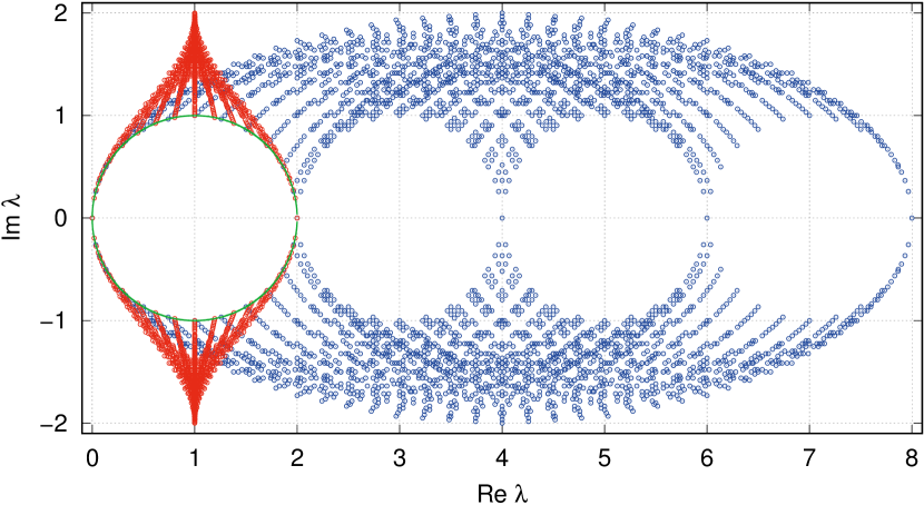
Figure 1: Eigenvalue spectrum of the staggered Wilson (red) and the Wilson Dirac operator (blue) in the free-field case together with the Ginsparg-Wilson circle (green).

For Wilson and staggered Wilson fermions, the free-field eigenvalue spectrum can be found in Fig. 1. As one can see, the staggered Wilson spectrum is close to the Ginsparg-Wilson circle and we have a clear separation between the physical and the doubler branch. Together with the fact that the staggered Wilson fermion matrix is smaller than the Wilson fermion matrix, one expects a significant computational advantage for staggered overlap fermions. This was confirmed by the free-field speedup factor of $\mathcal{O}\left(10\right)$ in the studies of Refs. [70, 71].

3 Quenched quantum chromodynamics

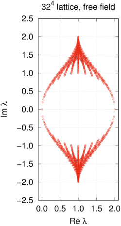
(a) $32^{4}$ lattice, free field

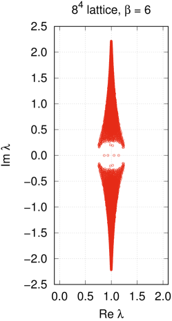
(b) $8^{4}$ lattice at $\beta=6$

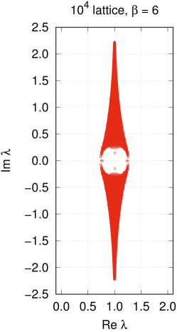
(c) $10^{4}$ lattice at $\beta=6$

Figure 1: The staggered Wilson eigenvalue spectrum at $\beta=6$.

(a) $32^{4}$ lattice, free field

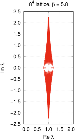
(b) $8^{4}$ lattice at $\beta=5.8$

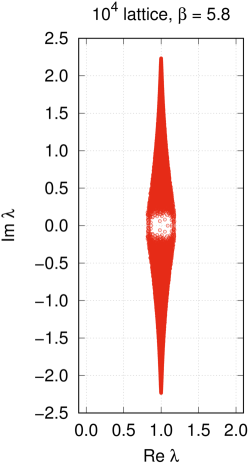
(c) $10^{4}$ lattice at $\beta=5.8$

Figure 2: The staggered Wilson eigenvalue spectrum at $\beta=5.8$.

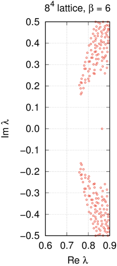
(a) $8^{4}$ lattice at $\beta=6$

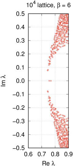
(b) $10^{4}$ lattice at $\beta=6$

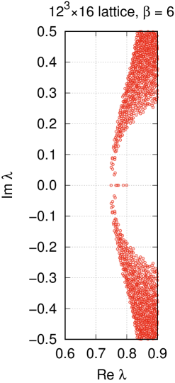
(c) $12^{3}\times 16$ lattice at $\beta=6$

Figure 3: Close-up of the physical branch of the staggered Wilson Dirac operator for increasing lattice sizes.

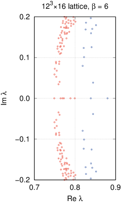
(a) $12^{3}\times 16$ lattice at $\beta=6$

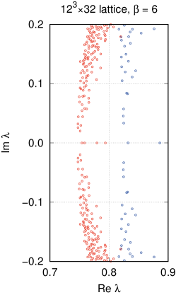
(b) $12^{3}\times 32$ lattice at $\beta=6$

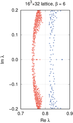
(c) $16^{3}\times 32$ lattice at $\beta=6$

Figure 4: Comparison of the staggered Wilson (red) and Wilson Dirac spectrum (blue).

Let us now consider the case of (unsmeared) quenched QCD background fields. The calculation of eigenvalue spectra on large lattices is numerically and computationally challenging. The Dirac operator is represented by a large, nonsymmetric, complex-valued matrix of size $\left(N_{\mathsf{c}}N_{\mathsf{d}}N_{\mathsf{s}}^{3}N_{\mathsf{t}}\right)^{2}$, where for quantum chromodynamics the number of colors is $N_{\mathsf{c}}=3$ and the number of spinor components is given by $N_{\mathsf{d}}=4$ for Wilson and by $N_{\mathsf{d}}=1$ for staggered Wilson fermions. In particular, for larger lattices such as a $N_{s}\times N_{t}=16^{3}\times 32$ lattice, we have more than $1.5\times 10^{6}$ eigenvalues for the Wilson Dirac operator and more than $5\times 10^{5}$ for the staggered Wilson Dirac operator. As a result, we can compute complete eigenvalue spectra only for small lattice sizes. For larger lattices, we have to restrict ourselves to subsets of the spectrum. Of particular interest is here the physically relevant low-lying part around the physical branch.

1 Implementation

To determine the eigenvalues of interest, our numerical implementation works as follows. For small lattices we compute complete eigenvalue spectra using the lapack [149] library. The library function zgeev computes all eigenvalues of a complex nonsymmetric matrix in double precision using the $QR$-algorithm [150, 151, 152]. As the function requires the input matrix to be constructed explicitly (i.e. densely) in memory, its use for larger lattices is limited by quickly growing memory requirements. As a consequence we use this method to compute complete spectra for lattices of up to a size of $6^{4}$ for the Wilson Dirac operator and up to a size of $10^{4}$ in the case of the staggered Wilson Dirac operator.

For larger lattices we use arpack [153], a library to solve large-scale eigenvalue problems involving sparse and structured matrices. It uses the implicitly restarted Arnoldi method [154] to compute the low-lying part of the eigenvalue spectrum. Here low-lying refers to eigenvalues with smallest absolute values. The implicitly restarted Arnoldi method is an iterative method and is not suitable for the computation of complete spectra, hence our choice of lapack for smaller lattices. It has nontrivial convergence behavior, in particular choosing the number of Lanczos basis vectors has significant impact on the performance. The znaupd function deals with the case of a complex nonsymmetric matrix in double precision. By choosing the bare mass parameter $m$ appropriately, one can shift the part of the spectrum of interest to the origin. With our setup we can compute typically a few hundred eigenvalues for lattice sizes of up to $16^{3}\times 32$ in quenched QCD background fields.

In the following, all reported numerical results are for periodic boundary conditions, use the canonical choice $r=1$ and are shifted back to $m=0$. All numerical calculations are done in double precision as the use of single precision resulted in erroneous eigenvalues due to accumulated rounding errors.

2 Eigenvalue spectra

We now begin our discussion of the eigenvalue spectra by comparing the free-field case with a $\beta=6$ quenched QCD background field on small lattices. In Fig. 1, we can find two typical examples for the spectrum for a $8^{4}$ and a $10^{4}$ lattice. Compared to the free-field spectrum in the same figure, we can see how the whole spectrum is contracted noticeably and the gap is narrow. In Ref. [70], this degradation of the spectrum was attributed to the four-hop terms in the staggered Wilson action, which raise gauge fluctuations to the fourth power. The physical branch and the doubler branch get closer as the spectrum collapses into a vertical stripe and one would expect a reduced computational efficiency of staggered Wilson fermions.

For $\beta=5.8$ the spectrum degrades further. In Fig. 2, we can find two exemplary eigenvalue spectra. We see that the branches become even more diffuse and the gap is very narrow. As a result, we expect a further decreased performance compared to the $\beta=6$ case.

The situation changes when we move to larger lattices. In Fig. 3, we can find a close-up of the physical branch over an increasing range of lattice sizes from $8^{4}$ to $12^{3}\times 16$ at $\beta=6$. We can observe how for larger lattices the physical branch becomes increasingly sharp. Finally, in Fig. 4 we can find a direct comparison of the physical branch of both the Wilson and staggered Wilson Dirac operator up to the largest lattices we can access, i.e. $16^{3}\times 32$. Here we can see very clearly how the spectrum improves from small to large lattices. While on small lattices the branches are diffuse and not well-separated, on larger lattices the situation improves remarkably.

4 Conclusions

Our observations give a possible explanation for the modest speedup factors for staggered overlap fermions observed in Refs. [70, 71] compared to the large speedup factors for staggered Wilson fermions found in Refs. [4, 7]. While the former study was carried out on small lattices up to a size of $12^{4}$, the latter one was done on lattices sizes of up to a size of $20^{3}\times 40$.

As we confirmed, on small lattices the eigenvalue spectrum has a small gap and is lacking a clear separation of the branches. Here one can often find eigenvalues close to the center of the “belly” of the spectrum, making the overlap construction computationally more expensive. The situation quickly improves on both the infrared and ultraviolet part of the spectrum when increasing the lattice size, see Fig. 3. While this also holds for Wilson fermions, it appears to be more pronounced for the staggered Wilson Dirac operator, which is likely linked to the presence of four-hop terms in the staggered Wilson term.

That the eigenvalue spectrum of the staggered Wilson Dirac operator is well-behaved on larger lattices can also be seen from the condition number. The diffuse spectrum could in principle give rise to almost vanishing eigenvalues when the pion mass is small. However, as we observed the condition number in our numerical studies in Sec. 3 to be typically a factor of $\mathcal{O}\left(4\right)$ smaller compared to Wilson fermions, we conclude that these pathological cases are rare.

Finally the smaller additive mass renormalization of staggered Wilson fermions is suggesting improved chiral properties compared to Wilson fermions, which are expected to have a positive impact on the computational efficiency.

As a consequence, we believe that the speedup factors reported in Refs. [70, 71] are not representative for the actual performance gains achievable with staggered overlap fermions on larger lattices. We would expect a higher computational efficiency in cases where the staggered Wilson eigenvalue spectrum shows a wide gap and well-separated, sharp branches. As our study suggests, this can be (at least partially) achieved by moving to larger lattices, although only a comprehensive numerical study can clarify this point in the end. Alternatively, as suggested in Ref. [82], smearing also significantly improves the eigenvalue spectrum and, thus, is expected to result in an improved computational performance.

Chapter 7 Staggered domain wall fermions

Besides staggered overlap fermions, the staggered Wilson kernel allows the construction of a related chiral lattice formulation, namely staggered domain wall fermions as proposed by Adams in Refs. [44, 45]. In the following, we investigate spectral properties and quantify chiral symmetry violations of various formulations of staggered and usual domain wall fermions. We do this in the free-field case, on quenched thermalized background fields in the setting of the Schwinger model and on smooth topological configurations. Moreover, we present first results for four-dimensional quantum chromodynamics. We closely follow the discussion from our original and subsequent reports given in Refs. [2, 12, 1], where we previously presented our results.

1 Introduction

For our understanding of the low-energy dynamics of quantum chromodynamics, such as hadron phenomenology, chiral symmetry plays an essential role. While the proper implementation of chiral symmetry on the lattice turned out to be a notorious problem, it was eventually overcome with the overlap construction as discussed in Chapter 5. Overlap fermions obey an exact chiral symmetry, thus evading the Nielsen-Ninomiya theorem (cf. Subsec. 4). From a theoretical perspective overlap fermions have many desirable properties, but their practical use is limited due to the fact that they typically require a factor of $\mathcal{O}\left(10\text{--}100\right)$ more computational resources compared to Wilson fermions. Moreover, even at moderate lattice spacings tunneling between topological sectors is strongly suppressed [155, 156, 157, 158], so that adequate coverage of the different topological sectors becomes a concern.

An alternative to overlap fermions is given by domain wall fermions [159, 160, 161], which implement an approximate chiral symmetry in $d$ dimensions by means of a theory of massive coupled fermions in $d+1$ dimensions ($d=2,4$). The extent of this extra dimension controls the degree of chiral symmetry violations and in the limit of an infinite extent one recovers the overlap operator with its exact chiral symmetry. The case of a finite extent can be interpreted as a truncation of overlap fermions.

Implementations of domain wall fermions can be easily parallelized and bear the potential of reduced computational costs. While they only have an approximate chiral symmetry, violations of chiral symmetry are well-controlled. Based on theoretical grounds, these violations are expected to be exponentially suppressed [160, 162, 163, 164]. In practice, however, this suppression typically still requires large extents of the extra dimension [165, 166, 167, 168, 169]. At the same time, these violations allow for an easier tunneling between different topological sectors.

Typically domain wall fermions are formulated with a Wilson-like kernel operator. However, recently Adams laid the foundations [44, 45] for the use of staggered kernels in the domain wall construction. This was enabled by the introduction of a flavored mass term as described in Sec. 4. While in previous studies the properties of the staggered Wilson kernel [79, 80, 81, 71, 82, 4] and the staggered overlap construction [45, 70, 3] were investigated, the staggered domain wall fermion formulation was largely ignored in the literature. For this reason, we investigate Adams’ proposal in this chapter. We give explicit constructions of these lattice fermions in different variants, study their spectral properties and compare the degree of chiral symmetry breaking with the one of usual domain wall fermions in the setting of the Schwinger model [170].

The Schwinger model, i.e. quantum electrodynamics (QED) in two dimensions, serves us a toy-model for quantum chromodynamics (QCD). Like quantum chromodynamics itself, it shows confinement and has topological structure. At the same time its numerical treatment is simpler and allows the computation of complete eigenvalue spectra of lattice Dirac operators on nontrivial background fields. Moreover, the study of the Schwinger model is of interest in its own right as it is relevant for the description of conducting electrons in metals in the low-energy regime, see e.g. Ref. [171].

This chapter is organized as follows. In Sec. 2, we give a short overview of the kernel operators we use in our study. In Sec. 3, we discuss the construction of (staggered) domain wall fermions and their variants. In Sec. 4, we introduce effective low-energy Dirac operators and discuss their relations to the overlap formalism. In Sec. 5, we introduce the setting of our numerical calculations. In Sec. 6, we discuss the numerical results in detail. In Sec. 7, we present first results for four-dimensional quantum chromodynamics. In Sec. 8, we provide some exemplary weight factors for the optimal domain wall construction and finally in Sec. 9, we end with some concluding remarks.

2 Kernel operators

Throughout this chapter we consider domain wall fermions with two different kernel operators, i.e. Wilson and staggered Wilson fermions. In the following, we adopt the notation previously used in Chapters 1, 2 and 5. In the case of $d=2$ dimensions the $\gamma_{\mu}\in\mathbb{C}^{2\times 2}$ matrices ($\mu=1,2$) correspond to a representation of the Dirac algebra $\left\{\gamma_{\mu},\gamma_{\nu}\right\}=2\delta_{\mu\nu}\mathbbm{1}$ and we denote the chirality matrix as $\gamma_{3}$. At the same time, the $\xi_{\mu}\in\mathbb{C}^{2\times 2}$ matrices are a representation of the Dirac algebra in flavor space.

Wilson fermions.

We introduced and discussed the Wilson Dirac operator in Subsec. 6. The Dirac operator is defined in Eq. (21), where we consider the case of two space-time dimensions for our numerical studies.

Staggered Wilson fermions.

The second kernel operator of interest is Adams’ staggered Wilson Dirac operator. In Sec. 4 and Sec. 6, we discussed its construction and properties in detail. In the numerical part of this chapter we use the formulation in $d=2$ dimensions as defined in Eq. (20). We note that in principle also the use of the other flavored mass terms in Chapter 2 can give rise to suitable kernel operators.

3 Domain wall fermions

Domain wall fermion were originally proposed by Kaplan in Ref. [159] and subsequently refined by Shamir and Furman in Refs. [160, 161]. By means of a $\left(d+1\right)$-dimensional theory, the domain wall formulation realizes approximately massless fermions in $d$ dimensions. Alternatively, one can interpret the construction as a tower of $N_{s}$ fermions in $d$ dimensions with a specific flavor structure.

We begin by introducing the $\left(d+1\right)$-dimensional bulk operators, where we fix the lattice spacing to $a=1$ in the first $d$ dimensions and the (staggered) Wilson parameter to $r=1$. Although for the numerical work we are interested in the $d=2$ setting, we keep the following discussion general and consider the case of even $d$ dimensions, where $\gamma_{d+1}$ refers to the corresponding chirality matrix in that dimension.

1 Standard construction

We begin with the originally proposed construction. We define

$$D_{\mathsf{w}}^{\pm}=a_{d+1}D_{\mathsf{w}}\left(-M_{0}\right)\pm\mathbbm{1}$$ (1)

and explicitly keep the lattice spacing $a_{d+1}$ in the extra dimension. The mass parameter $M_{0}$ is commonly referred to as the domain wall height and has to be suitably chosen to give rise to a one flavor theory. For the free-field case, its values are restricted to the range $M_{0}\in\left(0,2r\right)$.

We can write down the Dirac operator, which reads

$$\overline{\Psi}D_{\mathsf{dw}}\Psi=\sum_{s=1}^{N_{s}}\overline{\Psi}_{s}\left[D_{\mathsf{w}}^{+}\Psi_{s}-P_{-}\Psi_{s+1}-P_{+}\Psi_{s-1}\right]$$ (2)

with chiral projectors $P_{\pm}=\left(\mathbbm{1}\pm\gamma_{d+1}\right)/2$ and $\left(d+1\right)$-dimensional fermion fields $\overline{\Psi}$, $\Psi$. Throughout this chapter, the index $s=1,\dots,N_{s}$ refers to the additional spatial coordinate (or equivalently to the flavor). Along the extra spatial coordinate, the gauge links are taken to be the unit matrix. Furthermore, for finite extents of the $s$-coordinate we must impose boundary conditions, which we take to be

$$P_{+}\left(\Psi_{0}+m\Psi_{N_{s}}\right) =0,$$ (3)

$$P_{-}\left(\Psi_{N_{s}+1}+m\Psi_{1}\right) =0.$$

Here the parameter $m$ is related to the bare fermion mass, see Eq. (8). In the special case of $m=0$ the condition reduces to Dirichlet type boundary conditions, while for $m=\pm 1$ we find (anti-)periodic boundary conditions. Writing the Dirac operator explicitly in the extra dimension, we find

$$D_{\mathsf{dw}}=\left(\begin{array}[]{ccccc}D_{\mathsf{w}}^{+}&-P_{-}&&&mP_{+}\\ -P_{+}&D_{\mathsf{w}}^{+}&-P_{-}\\ &\ddots&\ddots&\ddots\\ &&-P_{+}&D_{\mathsf{w}}^{+}&-P_{-}\\ mP_{-}&&&-P_{+}&D_{\mathsf{w}}^{+}\end{array}\right).$$ (4)

The $d$-dimensional fermion fields can be defined from the boundary as

$$q =P_{+}\Psi_{N_{s}}+P_{-}\Psi_{1},$$ (5)

$$\overline{q} =\overline{\Psi}_{1}P_{+}+\overline{\Psi}_{N_{s}}P_{-}.$$

Now let us also introduce the reflection operator in the extra dimension

$$R=\left(\begin{array}[]{ccc}&&\mathbbm{1}\\ &\iddots\\ \mathbbm{1}\end{array}\right).$$ (6)

We can easily verify that $D_{\mathsf{dw}}$ is $R\gamma_{d+1}$ Hermitian, that is

$$D_{\mathsf{dw}}^{\dagger}=R\gamma_{d+1}\cdot D_{\mathsf{dw}}\cdot R\gamma_{d+1}.$$ (7)

This property implies the reality of the fermion determinant, i.e. $\det D_{\mathsf{dw}}\in\mathbb{R}$.

Besides this standard formulation, several variants of domain wall fermions have been proposed after the original proposal.

2 Boriçi’s construction

Among them we can find Boriçi’s construction [172], which follows from the standard construction by the replacements

$$P_{+}\Psi_{s-1} \to-D_{\mathsf{w}}^{-}P_{+}\Psi_{s-1},$$ (8)

$$P_{-}\Psi_{s+1} \to-D_{\mathsf{w}}^{-}P_{-}\Psi_{s+1}$$

and is an $\mathcal{O}\left(a_{d+1}\right)$ modification. After this replacement, the Dirac operator takes the form

$$\overline{\Psi}D_{\mathsf{dw}}\Psi=\sum_{s=1}^{N_{s}}\overline{\Psi}_{s}\left[D_{\mathsf{w}}^{+}\Psi_{s}+D_{\mathsf{w}}^{-}P_{-}\Psi_{s+1}+D_{\mathsf{w}}^{-}P_{+}\Psi_{s-1}\right]$$ (9)

or explicitly

$$D_{\mathsf{dw}}=\left(\begin{array}[]{ccccc}D_{\mathsf{w}}^{+}&D_{\mathsf{w}}^{-}P_{-}&&&-mD_{\mathsf{w}}^{-}P_{+}\\ D_{\mathsf{w}}^{-}P_{+}&D_{\mathsf{w}}^{+}&D_{\mathsf{w}}^{-}P_{-}\\ &\ddots&\ddots&\ddots\\ &&D_{\mathsf{w}}^{-}P_{+}&D_{\mathsf{w}}^{+}&D_{\mathsf{w}}^{-}P_{-}\\ -mD_{\mathsf{w}}^{-}P_{-}&&&D_{\mathsf{w}}^{-}P_{+}&D_{\mathsf{w}}^{+}\end{array}\right).$$ (10)

Moreover, the generalization of Eq. (5) reads

$$q =P_{+}\Psi_{N_{s}}+P_{-}\Psi_{1},$$ (11)

$$\overline{q} =-\overline{\Psi}_{1}D_{\mathsf{w}}^{-}P_{+}-\overline{\Psi}_{N_{s}}D_{\mathsf{w}}^{-}P_{-}$$

and the equivalent of Eq. (7) takes the form

$$\left(\mathcal{D}^{-1}D_{\mathsf{dw}}\right)^{\dagger} =R\gamma_{d+1}\cdot\left(\mathcal{D}^{-1}D_{\mathsf{dw}}\right)\cdot R\gamma_{d+1},$$ (12)

$$\mathcal{D} =\mathbbm{1}_{N_{s}}\otimes D_{\mathsf{w}}^{-}$$

(see Ref. [173]). Boriçi referred to this formulation as truncated overlap fermions due to the fact that the corresponding $d$-dimensional effective operator, as discussed in Sec. 4, corresponds to the polar decomposition approximation [107, 174] of Neuberger’s overlap operator of order $N_{s}/2$ (where $N_{s}$ is even).

3 Optimal construction

Another modification of domain wall fermions is the optimal construction as proposed by Chiu [175, 176]. Here one modifies $D_{\mathsf{dw}}$ so that the effective Dirac operator is formulated via Zolotarev’s optimal rational function approximation of the $\operatorname{sign}$ function [177, 178, 179], see also Refs. [117, 180]. We now summarize the construction given in Ref. [175].

As a starting point we use Boriçi’s formulation of domain wall fermions. We generalize the Dirac operator by introducing weight factors

$$\overline{\Psi}D_{\mathsf{dw}}\Psi=\sum_{s=1}^{N_{s}}\overline{\Psi}_{s}\left[D_{\mathsf{w}}^{+}\left(s\right)\Psi_{s}+D_{\mathsf{w}}^{-}\left(s\right)P_{-}\Psi_{s+1}+D_{\mathsf{w}}^{-}\left(s\right)P_{+}\Psi_{s-1}\right]$$ (13)

via

$$D_{\mathsf{w}}^{\pm}\left(s\right)=a_{d+1}\omega_{s}D_{\mathsf{w}}\left(-M_{0}\right)\pm\mathbbm{1}.$$ (14)

The weight factors $\omega_{s}$ take the values

$$\omega_{s}=\frac{1}{\lambda_{\mathsf{min}}}\sqrt{1-\kappa^{\prime 2}\operatorname{sn}\left(v_{s},\kappa^{\prime}\right)}$$ (15)

with $\operatorname{sn}\left(v_{s},\kappa^{\prime}\right)$ being the respective Jacobi elliptic function with the argument $v_{s}$ and modulus $\kappa^{\prime}$. The modulus is taken as

$$\kappa^{\prime}=\sqrt{1-\lambda_{\mathsf{min}}^{2}/\lambda_{\mathsf{max}}^{2}}$$ (16)

and $\lambda_{\mathsf{min}}^{2}$ ($\lambda_{\mathsf{max}}^{2}$) denotes the smallest (largest) eigenvalue of $H_{\mathsf{w}}^{2}$ with

$$H_{\mathsf{w}}=\gamma_{d+1}D_{\mathsf{w}}\left(-M_{0}\right).$$ (17)

The argument $v_{s}$ reads

$$v_{s}=\left(-1\right)^{s-1}M\operatorname{sn}^{-1}\left(\sqrt{\frac{1+3\lambda}{\left(1+\lambda\right)^{3}}},\sqrt{1-\lambda^{2}}\right)+\left\lfloor\frac{s}{2}\right\rfloor\frac{2K^{\prime}}{N_{s}},$$ (18)

where

$$\lambda =\prod_{\ell=1}^{N_{s}}\frac{\Theta^{2}\left(2\ell K^{\prime}/N_{s},\kappa^{\prime}\right)}{\Theta^{2}\left(\left(2\ell-1\right)K^{\prime}/N_{s},\kappa^{\prime}\right)},$$ (19)

$$M =\prod_{\ell=1}^{\left\lfloor N_{s}/2\right\rfloor}\frac{\operatorname{sn}^{2}\left(\left(2\ell-1\right)K^{\prime}/N_{s},\kappa^{\prime}\right)}{\operatorname{sn}^{2}\left(2\ell K^{\prime}/N_{s},\kappa^{\prime}\right)}.$$ (20)

Here $\left\lfloor\cdot\right\rfloor$ denotes the floor function, $K^{\prime}=K\left(\kappa^{\prime}\right)$ is the complete elliptic integral of the first kind with

$$K\left(k\right)=\intop_{0}^{\pi/2}\frac{\mathrm{d}\theta}{\sqrt{1-k^{2}\sin^{2}\theta}}.$$ (21)

We also introduced the elliptic Theta function via

$$\Theta\left(w,k\right)=\vartheta_{4}\left(\frac{\pi w}{2K},k\right)$$ (22)

with $K=K\left(k\right)$ and elliptic theta functions $\vartheta_{i}$, see e.g. Ref. [181]. To allow for the verification of implementations of these so-called optimal domain wall fermions, we provide some reference values for the weight factors $\omega_{s}$ in Sec. 8.

In the optimal construction, Eq. (5) is replaced by

$$q =P_{+}\Psi_{N_{s}}+P_{-}\Psi_{1},$$ (23)

$$\overline{q} =-\overline{\Psi}_{1}D_{\mathsf{w}}^{-}\left(1\right)P_{+}-\overline{\Psi}_{N_{s}}D_{\mathsf{w}}^{-}\left(N_{s}\right)P_{-}$$

and Eq. (7) again takes the form of Eq. (12), but now with

$$\mathcal{D}=\operatorname{diag}\left[D_{\mathsf{w}}^{-}\left(1\right),\dots,D_{\mathsf{w}}^{-}\left(N_{s}\right)\right]$$ (24)

as pointed out in Ref. [173]. Optimal domain wall fermions are one of the most popular domain wall fermion formulations and were used in numerous studies. In Refs. [182, 183, 184, 185, 186, 187] some of these works can be found.

Besides the original optimal domain wall fermion formulation, there is also a modified version [188] which is reflection-symmetric along the extra dimension. Finally, we note that all of the preceding domain wall fermion variants can be interpreted as special cases of Möbius domain wall fermions [173, 189, 190].

4 Staggered formulations

As recently clarified by Adams, it is possible to employ a staggered kernel for the formulation of domain wall fermions [44, 45]. Following this idea, the Dirac operator takes the form

$$\overline{\Upsilon}D_{\mathsf{sdw}}\Upsilon=\sum_{s=1}^{N_{s}}\overline{\Upsilon}_{s}\left[D_{\mathsf{sw}}^{+}\Upsilon_{s}-P_{-}\Upsilon_{s+1}-P_{+}\Upsilon_{s-1}\right],$$ (25)

where $\Upsilon$ refers to the $\left(d+1\right)$-dimensional staggered fermion field. Similarly to the Wilson case, we let

$$D_{\mathsf{sw}}^{\pm}=a_{d+1}D_{\mathsf{sw}}\left(-M_{0}\right)\pm\mathbbm{1}$$ (26)

with $D_{\mathsf{sw}}$ being the staggered Wilson Dirac operator. The chiral projectors are given by $P_{\pm}=\left(\mathbbm{1}\pm\epsilon\right)/2$, where $\epsilon$ is defined in Eq. (18) and we note that $\epsilon^{2}=\mathbbm{1}$. Recall that $\epsilon\sim\gamma_{d+1}\otimes\xi_{d+1}$, which reduces to $\epsilon\sim\gamma_{d+1}\otimes\mathbbm{1}$ on the physical species. The $R\gamma_{d+1}$ Hermiticity of $D_{\mathsf{dw}}$ generalizes to a $R\epsilon$ Hermiticity of $D_{\mathsf{sdw}}$. With our sign convention $D_{\mathsf{sdw}}$ is in full analogy with $D_{\mathsf{dw}}$, while a slightly different convention was used in the original proposal in Ref. [45].

In Ref. [45], a replacement rule was specified, which can be written in our general $d$-dimensional setting as

$$\gamma_{d+1}\to\epsilon,\qquad D_{\mathsf{w}}\to D_{\mathsf{sw}}$$ (27)

and describes how $D_{\mathsf{sdw}}$ can be constructed from $D_{\mathsf{dw}}$. Using Eq. (27), it is possible for us to generalize also Boriçi’s and Chiu’s work to the case of a staggered Wilson kernel. This allows us to write down the Dirac operator for what we are going to denote as truncated staggered domain wall fermions and which reads

$$\overline{\Upsilon}D_{\mathsf{sdw}}\Upsilon=\sum_{s=1}^{N_{s}}\overline{\Upsilon}_{s}\left[D_{\mathsf{sw}}^{+}\Upsilon_{s}+D_{\mathsf{sw}}^{-}P_{-}\Upsilon_{s+1}+D_{\mathsf{sw}}^{-}P_{+}\Upsilon_{s-1}\right].$$ (28)

Moreover, the Dirac operator of optimal staggered domain wall fermions, a generalization of Chiu’s construction, takes the form

$$\overline{\Upsilon}D_{\mathsf{sdw}}\Upsilon=\sum_{s=1}^{N_{s}}\overline{\Upsilon}_{s}\left[D_{\mathsf{sw}}^{+}\left(s\right)\Upsilon_{s}+D_{\mathsf{sw}}^{-}\left(s\right)P_{-}\Upsilon_{s+1}+D_{\mathsf{sw}}^{-}\left(s\right)P_{+}\Upsilon_{s-1}\right].$$ (29)

Here we let $D_{\mathsf{sw}}^{\pm}\left(s\right)=a_{d+1}\omega_{s}D_{\mathsf{sw}}\left(-M_{0}\right)\pm\mathbbm{1}$ and the weight factors $\omega_{s}$ are given by Eq. (15) for the kernel $H_{\mathsf{sw}}=\epsilon D_{\mathsf{sw}}\left(-M_{0}\right)$.

4 Effective Dirac operator

We now discuss the effective low-energy $d$-dimensional Dirac operator derived in Refs. [191, 192, 193, 172] (cf. Refs. [194, 195]). This will shine some light on the relation between the light $d$-dimensional $q$, $\overline{q}$ fields at the boundary and the $\left(d+1\right)$-dimensional theory. We follow Refs. [192, 172, 195] in our brief discussion of the construction.

1 Derivation

After integrating out the $N_{s}-1$ heavy modes in the theory, one can define an effective low-energy $d$-dimensional action

$$S_{\mathsf{eff}}=\sum_{x}\overline{q}\left(x\right)D_{\mathsf{eff}}\,q\left(x\right),$$ (1)

where the effective Dirac operator is defined by means of the propagator of light modes

$$D_{\mathsf{eff}}^{-1}\left(x,y\right)=\left\langle q\left(x\right)\overline{q}\left(y\right)\right\rangle.$$ (2)

In the $\left(d+1\right)$-dimensional theory we find one light and $N_{s}-1$ heavy Dirac fermions (for suitable choices of $M_{0}$).

If we take the chiral limit, where at fixed bare coupling $\beta$ we take the extent of the extra dimension to infinity $N_{s}\to\infty$, the contribution from the heavy modes diverges. This bulk contribution can be canceled by the introduction of pseudofermionic fields, where the pseudofermion action is typically taken to be the fermion action with $m=1$.

Now let us define the Hermitian operators

$$H_{\mathsf{w}}=\gamma_{d+1}D_{\mathsf{w}}\left(-M_{0}\right),\qquad H_{\mathsf{m}}=\gamma_{d+1}D_{\mathsf{m}}\left(-M_{0}\right),$$ (3)

where for standard domain wall fermions the kernel operator reads

$$D_{\mathsf{m}}\left(-M_{0}\right)=\frac{D_{\mathsf{w}}\left(-M_{0}\right)}{2\cdot\mathbbm{1}+a_{d+1}D_{\mathsf{w}}\left(-M_{0}\right)}.$$ (4)

The transfer matrix in the extra dimension takes the form

$$T=\frac{T_{-}}{T_{+}},\qquad T_{\pm}=\mathbbm{1}\pm a_{d+1}H,$$ (5)

where the Hermitian operator $H$ depends on the construction given by

$$H=\begin{cases}H_{\mathsf{m}}&\textrm{for standard construction},\\ H_{\mathsf{w}}&\textrm{for Boriçi's construction}.\end{cases}$$ (6)

One can derive the explicit form [192] of the effective Dirac operator to find

$$D_{\mathsf{eff}}=\frac{1+m}{2}\mathbbm{1}+\frac{1-m}{2}\gamma_{d+1}\frac{T_{+}^{N_{s}}-T_{-}^{N_{s}}}{T_{+}^{N_{s}}+T_{-}^{N_{s}}}.$$ (7)

Rewriting Eq. (7) as

$$D_{\mathsf{eff}}=\left(1-m\right)\left[D_{\mathsf{eff}}\left(0\right)+\frac{m}{1-m}\right],$$ (8)

where $D_{\mathsf{eff}}\left(0\right)$ refers to the effective operator $D_{\mathsf{eff}}$ at $m=0$, we find a bare mass of $m/\left(1-m\right)$ for a given choice of the parameter $m$, see Ref. [196].

The effective operator in Eq. (7) can also be written in the compact form

$$D_{\mathsf{eff}}=\left(\mathcal{P}^{\intercal}D_{1}^{-1}D_{m}\mathcal{P}\right)_{1,1}$$ (9)

as shown in Refs. [172, 195], where the matrix $\mathcal{P}$ reads

$$\mathcal{P}=\left(\begin{array}[]{ccccc}P_{-}&P_{+}\\ &P_{-}&P_{+}\\ &&\ddots&\ddots\\ &&&P_{-}&P_{+}\\ P_{+}&&&&P_{-}\end{array}\right)$$ (10)

and $\mathcal{P}^{-1}=\mathcal{P}^{\intercal}$. To simplify the notation we introduced $D_{m}\equiv D_{\mathsf{dw}}\left(m\right)$ and the $\left(1,1\right)$-index refers to the corresponding $s$-block of the matrix product.

For Chiu’s optimal domain wall fermions the derivation follows Boriçi’s case, where the additional weight factors $\omega_{s}$ have to be taken into account [175]. By construction, we find that in this case the $\operatorname{sign}$-function approximation in the effective Dirac operator equals Zolotarev’s optimal rational function approximation.

2 The $N_{s}\to\infty$ limit

For the following discussion we restrict ourselves to the $m=0$ case. First, we remark that Eq. (7) can be written as

$$\frac{T_{+}^{N_{s}}-T_{-}^{N_{s}}}{T_{+}^{N_{s}}+T_{-}^{N_{s}}}=\epsilon_{N_{s}/2}\left(a_{d+1}H\right),$$ (11)

where $\epsilon_{N_{s}/2}$ is Neuberger’s polar decomposition approximation [107, 174] of the $\operatorname{sign}$-function. One can easily see that in the $N_{s}\to\infty$ limit we recover the overlap Dirac operator,

$$D_{\mathsf{ov}} =\lim_{N_{s}\to\infty}D_{\mathsf{eff}}$$

$$=\frac{1}{2}\mathbbm{1}+\frac{1}{2}\gamma_{d+1}\operatorname{sign}H$$

$$=\frac{1}{2}\left[\mathbbm{1}+D_{-M_{0}}\left(D_{-M_{0}}^{\dagger}D_{-M_{0}}\right)^{-\frac{1}{2}}\right],$$ (12)

with $H$ given in Eq. (6), using the shorthand notation $D_{-M_{0}}=D\left(-M_{0}\right)$ and

$$D=\begin{cases}D_{\mathsf{m}}&\textrm{for standard construction},\\ D_{\mathsf{w}}&\textrm{for Boriçi's/Chiu's construction}.\end{cases}$$ (13)

The Ginsparg-Wilson equation

$$\left\{\gamma_{d+1},D_{\mathsf{ov}}\right\}=2D_{\mathsf{ov}}\gamma_{d+1}D_{\mathsf{ov}}$$ (14)

can be shown to hold for $D_{\mathsf{ov}}$, thus implementing an exact chiral symmetry and implying the normality of the operator. We note that compared to the discussion in Subsec. 1, we find an additional factor of two in the Ginsparg-Wilson relation due to a different normalization of the overlap operator.

If we now compare Eq. (12) with the standard definition

$$D_{\mathsf{ov}}=\rho\left[\mathbbm{1}+D_{-\rho}\left(D_{-\rho}^{\dagger}D_{-\rho}\right)^{-\frac{1}{2}}\right]$$ (15)

of the overlap operator and we use the relation for the effective negative mass parameter

$$\rho=\begin{cases}M_{0}-\frac{a_{d+1}}{2}M_{0}^{2}&\textrm{for standard construction},\\ M_{0}&\textrm{for Boriçi's/Chiu's construction},\end{cases}$$ (16)

this would result in a restriction on the domain wall height $M_{0}$ from $\rho=1/2$. This limitation can be overcome by rescaling $D_{\mathsf{eff}}$ by a factor $\varrho=2\rho$, so that in the free-field case the low-lying eigenvalues of the kernel operator remain invariant (up to discretization effects) when the effective operator projection is applied. This can also be seen in Fig. 7, which we later discuss in Sec. 1. In all numerical investigations of this chapter this rescaling is taken into account.

3 Approximate sign functions

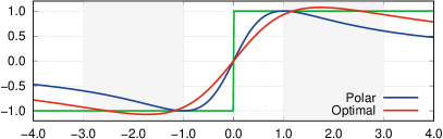
(a) $N_{s}=2$

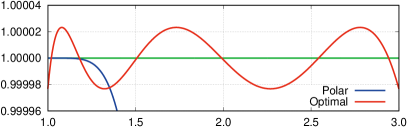
(b) $N_{s}=6$

Figure 1: Approximations of the $\operatorname{sign}$-function by $r\left(z\right)$. The optimal construction is illustrated for the case of $\lambda_{\mathsf{min}}=1$ and $\lambda_{\mathsf{max}}=3$.

The effective operator, as previously derived, is an approximation to the overlap operator. Explicitly, the $\operatorname{sign}$-function is approximated by the rational function

$$r\left(z\right)=\frac{\Pi_{+}\left(z\right)-\Pi_{-}\left(z\right)}{\Pi_{+}\left(z\right)+\Pi_{-}\left(z\right)}$$ (17)

with

$$\Pi_{\pm}\left(z\right)=\begin{cases}\left(1\pm z\right)^{N_{s}}&\textrm{for standard/Boriçi's construction},\\ \prod_{s}\left(1\pm\omega_{s}z\right)&\textrm{for Chiu's construction}.\end{cases}$$ (18)

As expected, we can verify that $r\left(z\right)\to\operatorname{sign}\left(z\right)$ for $N_{s}\to\infty$. We note that for the standard construction and Boriçi’s construction the approximation is identical, but is applied to different kernel operators, namely $H_{\mathsf{m}}$ or $H_{\mathsf{w}}$ respectively. To illustrate the approximations in Eq. (18), we compare the polar decomposition approximation in Boriçi’s formulation with the optimal approximation in Chiu’s construction in Fig. 1. As we can see, the approximation error over the construction range is significantly lower for the optimal construction. We recall that the coefficients $\omega_{s}$ are related to Zolotarev’s coefficients, cf. Refs. [177, 117, 180].

Staggered formulations

The discussion in this section naturally generalizes to the case of a staggered Wilson kernel, when the replacement rule in Eq. (27) is applied. In particular, the effective and overlap operators follow from this replacement and we can interpret staggered domain wall fermions as a truncation of staggered overlap fermions [45].

5 Setting

We now move on to the numerical part of the study and begin by discussing our setting. In particular, we elaborate on our method to quantify chiral symmetry violations to benchmark the various domain wall fermion constructions.

1 Setting the domain wall height

To give rise to a one-flavor theory, in the free-field case the domain wall height $M_{0}$ has to be chosen in the range $0<M_{0}<2r$. When moving to a nontrivial background field, this interval generally shifts and contracts. In less rigor terms, the parameter $M_{0}$ has to be chosen so that the origin is shifted inside the leftmost “belly” of the eigenvalue spectrum of the kernel operator. Although even in the free-field case there is no optimal choice for $M_{0}$ as discussed in Ref. [197], one typically uses the canonical choice $M_{0}=1$ for the free field, which is at the center of the eigenvalue belly. More rigorously speaking, valid choices of $M_{0}$ are restricted by the position of the mobility edge [198, 199, 200, 51].

In the Schwinger model, for reasonable choices of the inverse coupling $\beta$ the eigenvalue spectrum is not distorted too far away from the free-field spectrum. As a consequence, valid choices for $M_{0}$ remain close to the free-field case. While in four-dimensional quantum chromodynamics one often uses $M_{0}=1.8$ (see e.g. Ref. [201]), in our present case $M_{0}=1$ remains a sensible and simple choice, which we consequently use for all our numerical work.

2 Effective mass

Commonly employed measures in the literature to quantify the degree of chiral symmetry breaking of domain wall fermions are the residual mass $m_{\mathsf{res}}$ [161, 167, 201, 202] and the effective mass $m_{\mathsf{eff}}$ [203, 204, 205]. While the residual mass makes use of the explicit mass dependence in the chiral Ward-Takahashi identities, the effective mass is defined as the lowest eigenvalue (by magnitude) of the Hermitian operator in a background field with nontrivial topology. Although these measures are not identical, they usually agree within a factor of order $\mathcal{O}\left(1\right)$. Consequently both define valid measures to quantify the chirality of a given lattice fermion formulation.

Because of its conceptual simplicity, we use the effective mass $m_{\mathsf{eff}}$ as one of our measures for the numerical studies. To give a precise definition, we consider a given Dirac operator $D$ on a topologically nontrivial background configuration with periodic boundary conditions and define the effective mass $m_{\mathsf{eff}}$ as the lowest eigenvalue of the Hermitian kernel operator $H$. Explicitly, we let

$$m_{\mathsf{eff}}=\min_{\lambda\in\operatorname{spec}H}\left|\lambda\right|=\min_{\Lambda\in\operatorname{spec}D^{\dagger}D}\sqrt{\Lambda},$$ (1)

where we used the fact that $H^{2}=D^{\dagger}D$. For a normal operator $D$, this definition simplifies to $m_{\mathsf{eff}}=\min_{\lambda\in\operatorname{spec}D}\left|\lambda\right|$. For a non-normal operator, however, the eigenvalues of $D$ and $H$ are not directly related.

For gauge configurations with topological charge $Q\neq 0$, the existence of zero modes of $H$ is guaranteed in the continuum by the Atiyah-Singer index theorem [121, 122, 123, 124]. Similarly, the presence of zero modes of the overlap operator as defined in Eq. (12) can be shown as well [109, 110, 111]. For the effective Dirac operators these zero modes are approximate, but become exact in the $N_{s}\to\infty$ limit. The absolute value of the eigenvalues of these approximate zero modes can then serve as a measure of chirality.

In the context of a gauge theory, the Atiyah-Singer index theorem takes the following form. Let $n_{\mp}$ refer to the number of left-handed and right-handed zero modes, then their difference is related to the topological charge by

$$n_{-}-n_{+}=\left(-1\right)^{d/2}Q,$$ (2)

see Ref. [44]. In Eq. (6), we will give a precise definition of $Q$. We note that one can show the Vanishing Theorem [125, 126, 127] in our two-dimensional setting. The theorem states that on gauge configurations with $Q\neq 0$, either $n_{-}$ or $n_{+}$ vanishes, i.e. $n_{-}$ and $n_{+}$ are not simultaneously nonzero.

3 Normality and Ginsparg-Wilson relation

The continuum Dirac operator, the naïve and overlap lattice Dirac operators are all normal operators. At the same time, the effective Dirac operators are not normal. This makes operator normality an interesting aspect in the context of chirality, especially as it has been shown that chiral properties imply the normality of the Dirac operator [206], see also Refs. [207, 208].

By definition a normal operator $D$ satisfies $\left[D,D^{\dagger}\right]=0$. Deviation from normality can be quantified by the norm of this commutator and we define

$$\Delta_{\mathsf{N}}=\left\|\left[D,D^{\dagger}\right]\right\|_{\infty},$$ (3)

where $\left\|\cdot\right\|_{\infty}$ is the matrix norm induced by the $L_{\infty}$-norm. As previously discussed, the normality measure $\Delta_{\mathsf{N}}$ vanishes for the overlap operator and, thus, for the effective Dirac operators in the limit $N_{s}\to\infty$.

Besides normality, violations of the Ginsparg-Wilson relation as given in Eq. (14) are a natural measure for chirality of a lattice fermion formulation. We let

$$\Delta_{\mathsf{GW}}=\left\|\left\{\gamma_{3},D\right\}-\rho^{-1}D\gamma_{3}D\right\|_{\infty}$$ (4)

and find that for the effective operators $\Delta_{\mathsf{GW}}\to 0$ for $N_{s}\to\infty$. For a staggered Wilson kernel, the chirality matrix $\gamma_{3}$ has to be replaced by the staggered $\epsilon$ in the definition of $\Delta_{\mathsf{GW}}$. We note that the additional factor of $1/\rho$ in Eq. (4) is due to the different scales of the effective Dirac operators. The measures $\Delta_{\mathsf{N}}$ and $\Delta_{\mathsf{GW}}$ were previously considered in Refs. [197, 209] and together with $m_{\mathsf{eff}}$ serve here as a measure for chiral symmetry violations.

4 Topological charge

To determine the topological charge of a gauge configuration, we use the index formula for the standard overlap operator,

$$Q=\frac{1}{2}\operatorname{Tr}\left(H_{\mathsf{w}}/\sqrt{H_{\mathsf{w}}^{2}}\right),$$ (5)

and its staggered equivalent,

$$Q=\frac{1}{2}\operatorname{Tr}\left(H_{\mathsf{sw}}/\sqrt{H_{\mathsf{sw}}^{2}}\right),$$ (6)

with $H_{\mathsf{sw}}=\epsilon D_{\mathsf{sw}}\left(-M_{0}\right)$ as discussed in Ref. [44]. We numerically verified that these two definition yield the same topological charge on a set of sample configurations. This observation is in agreement with analytical results [3] and other numerical studies [71, 210].

6 Numerical results

For the numerical part of this work, we calculate complete eigenvalue spectra and evaluate our measures of chirality for the previously discussed Dirac operators. We do this on various gauge configurations in the Schwinger model and cover the free-field case, thermalized configurations and the smooth topological configurations discussed in Ref. [211].

Throughout this section, we set the lattice spacings in all dimensions to $a=a_{d+1}=1$ and fix the (staggered) Wilson parameter to $r=1$. For the extra dimension we consider extents within the range $2\leq N_{s}\leq 8$. In order to allow the calculation of the effective mass $m_{\mathsf{eff}}$ as discussed in Sec. 2, we impose periodic boundary conditions in all dimensions.

We determine complete eigenvalue spectra using the lapack [149] library, while extremal eigenvalues, such as the effective mass, are computed with arpack [153]. For all numerical calculations we use double precision. In the figures, the standard construction is abbreviated with “std”, Boriçi’s construction with “Bor” and Chiu’s optimal construction with “opt”. When discussing overlap operators, the construction with kernel $H_{\mathsf{m}}$ is referred to as “DW”, Neuberger’s overlap with kernel $H_{\mathsf{w}}$ is abbreviated as “Neub” and Adams’ staggered overlap with kernel $H_{\mathsf{sw}}$ is denoted as “Adams”.

1 Free-field case

In our discussion we begin with the simplest case of the free field. Periodicity allows a Fourier transformation of the kernel operators and simplifies the computation of the eigenvalue spectra, cf. Chapter 6. In the momentum representation, the Wilson kernel takes the form of the following $2\times 2$ linear map

$$D_{\mathsf{w}}=\left(m_{\mathsf{f}}+2r\right)\mathbbm{1}+\textrm{i}\sum_{\mu}\gamma_{\mu}\sin p_{\mu}-r\sum_{\nu}\cos p_{\nu}\mathbbm{1},$$ (1)

where $p_{\mu}=2\pi n_{\mu}/N_{\mu}$ with $n_{\mu}=0,1,\dots,N_{\mu}-1$ and $N_{\mu}$ denotes the number of slices in $\mu$-direction. The staggered Wilson kernel is represented by the $4\times 4$ linear map

$$D_{\mathsf{sw}}=m_{\mathsf{f}}\left(\mathbbm{1}\otimes\mathbbm{1}\right)+\textrm{i}\sum_{\mu}\sin p_{\mu}\left(\gamma_{\mu}\otimes\mathbbm{1}\right)+r\mathbbm{1}\otimes\left(\mathbbm{1}+\xi_{3}\prod_{\nu}\cos p_{\nu}\right)$$ (2)

with $n_{\mu}=0,1,\dots,N_{\mu}/2-1$, cf. Ref. [71].

For the three-dimensional bulk operator, the extra dimension is lacking periodicity and we leave the corresponding coordinate in the position-space representation. By employing a momentum-space representation for the kernel operators, we reduce the dimensionality of the problem and avoid numerical instabilities otherwise encountered in the free-field case. All free-field results discussed in the following are for the case of a $N_{s}\times N_{t}=20\times 20$ lattice.

Kernel operators.

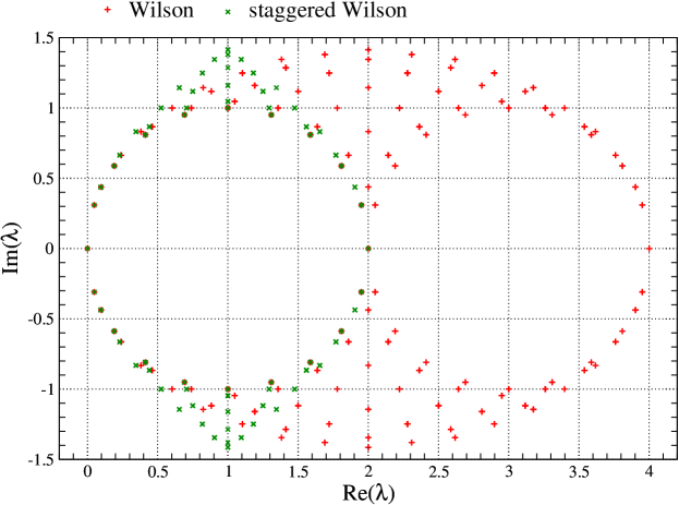
Figure 1: Spectrum of the kernel operators in the free field case.

In Fig. 1, we show the free-field eigenvalue spectra of the Wilson and staggered Wilson Dirac operator. While in four dimensions Wilson fermions have four doubler branches, in our setting of the two-dimensional Schwinger model only two doubler branches are present. Adams’ staggered Wilson term, however, always splits the tastes into two groups with positive and negative flavor-chirality. Compared to Wilson fermions, we observe how the spectrum of the staggered Wilson kernel resembles the Ginsparg-Wilson circle much more closely. On sufficiently smooth configurations one can then hope for lower computational costs for the construction of chiral fermion formulations.

We note that the Wilson and staggered Wilson eigenvalue spectrum differs mostly in their ultraviolet parts and very little in the physically relevant low-lying part. Nevertheless, these discretization effects alter the properties and shape of the bulk, effective and overlap operators and in general have an impact on computational efficiency and chiral properties.

Bulk operators.

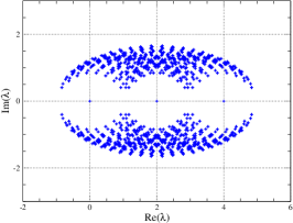
(a) Standard construction

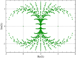
(b) Boriçi’s construction

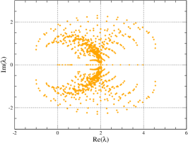
(c) Optimal construction

Figure 2: Spectrum of $D_{\mathsf{dw}}$ with Wilson kernel for $m=0$ at $N_{s}=8$ in the free field case.

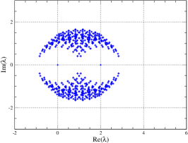
(a) Standard construction

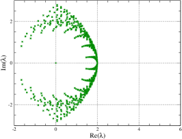
(b) Boriçi’s construction

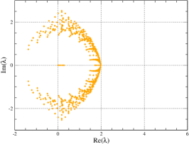
(c) Optimal construction

Figure 3: Spectrum of $D_{\mathsf{sdw}}$ with staggered Wilson kernel for $m=0$ at $N_{s}=8$ in the free field case.

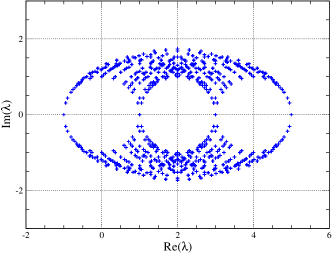
(a) Periodic case ($m=-1$)

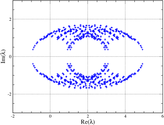
(b) Antiperiodic case ($m=1$)

Figure 4: Spectrum of $D_{\mathsf{dw}}$ with Wilson kernel in the standard construction at $N_{s}=8$ in the free field case with different boundary conditions (cf. Fig. 2)

Moving on to the $\left(2+1\right)$-dimensional bulk operators, in Figs. 2 and 3 we show the eigenvalue spectra in the standard, Boriçi’s and Chiu’s construction. To illustrate the effect of changing boundary conditions in the extra dimension, we show in Fig. 4 the case of periodic ($m=-1$) and antiperiodic ($m=1$) boundary conditions, which can be compared to the Dirichlet ($m=0)$ case.

In the spectrum of the bulk operator with the standard construction, we find (two) three doubler branches for the case of a (staggered) Wilson kernel. For Boriçi’s construction the number of branches is reduced by one. In both cases we find $2N_{s}$ exact zero modes in the Dirichlet case [160, 203], which disappear for non-vanishing values of $m$. For Chiu’s optimal construction we only find two approximate zero modes and observe that the real eigenvalues are spread along the real axis. In the case of Boriçi’s and the optimal construction with a Wilson kernel, we notice how the spectrum of the bulk operators lost its resemblance to the three-dimensional Wilson operator.

Effective operators.

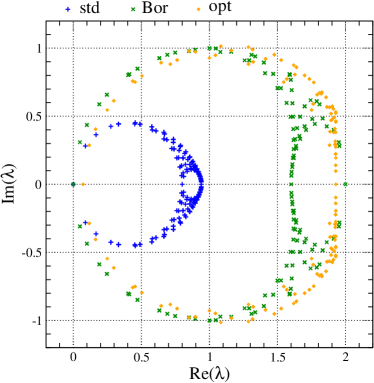
(a) Wilson kernel

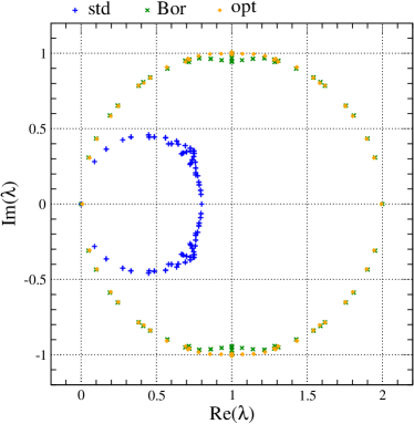
(b) Staggered Wilson kernel

Figure 5: Spectrum of $\varrho D_{\mathsf{eff}}$ for the standard (std), Boriçi (Bor) and optimal (opt) construction at $N_{s}=2$.

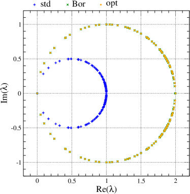
(a) Wilson kernel

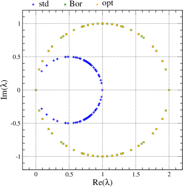
(b) Staggered Wilson kernel

Figure 6: Spectrum of $\varrho D_{\mathsf{eff}}$ for the standard (std), Boriçi (Bor) and optimal (opt) construction at $N_{s}=8$.

In Figs. 5 and 6, we can find the eigenvalue spectra of the effective Dirac operators $\varrho D_{\mathsf{eff}}$ with different kernel operators as defined in Eq. (7). The spectra resemble the Ginsparg-Wilson circle and rapidly converge towards it for increasing values of $N_{s}$. As the free field is smooth, this fast convergence is not unexpected. Already for small values of $N_{s}$ (such as $N_{s}=8$), it is almost impossible to visually distinguish the spectrum from the one of the associated overlap operator. We also point out the rapid convergence of Boriçi’s and Chiu’s construction, in particular with a staggered Wilson kernel.

By construction, the optimal construction shows significantly improved chiral properties. For a given spectral range $I=\left[\lambda_{\mathsf{min}},\lambda_{\mathsf{max}}\right]$ of the Hermitian kernel operator, the optimal rational function approximation $r_{\mathsf{opt}}\left(z\right)$ minimizes the maximal deviation from the $\operatorname{sign}$ function

$$\delta_{\mathsf{max}}=\max_{z\in-I\cup I}\left|\operatorname{sign}\left(z\right)-r_{\mathsf{opt}}\left(z\right)\right|=1\mp r_{\mathsf{opt}}\left(\pm\lambda_{\mathsf{min}}\right).$$ (3)

For a normal operator, such as in the free-field case, the eigenvalues are confined in a tube around the Ginsparg-Wilson circle with radius $\delta_{\mathsf{max}}$. As Zolotarev’s optimal approximation to the $\operatorname{sign}$-function minimizes the $\left\|\cdot\right\|_{\infty}$-norm, we find a point of maximal deviation at both $\lambda_{\mathsf{min}}$ and $\lambda_{\mathsf{max}}$, resulting in the absence of an exact zero mode. However, this approximate zero mode is decreasing rapidly in magnitude with increasing values of $N_{s}$ due to the rapid convergence of the underlying $\operatorname{sign}$-function approximation.

Overlap operators.

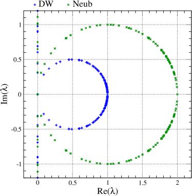
(a) Wilson kernel

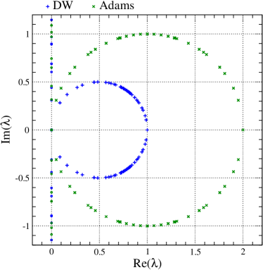
(b) Staggered Wilson kernel

Figure 7: Spectrum of $\varrho D_{\mathsf{ov}}$ with its stereographic projection for the domain wall (DW) kernel and the standard overlap (Neub/Adams) kernel.

Taking the $N_{s}\to\infty$ limit of the effective Dirac operators, we find an overlap operator. The Hermitian kernel operator $H$ of the overlap operator as given in Eq. (6) depends on the choice of the domain wall construction. In Fig. 7, we show the eigenvalue spectrum of $\varrho D_{\mathsf{ov}}$ together with the stereographic projection $\pi$ of the eigenvalues, given by the map

$$\pi\left(\lambda\right)=\frac{\lambda}{1-\frac{1}{\varrho}\lambda}.$$ (4)

The result is the projection of the eigenvalues onto the imaginary axis, where the physical low-lying eigenvalues line up as required due to the introduction of the scale factor in Eq. (16).

For Adams’ overlap operator the eigenvalue spectrum is highly symmetric. By construction, the effective operators in Boriçi’s and the optimal construction converge, depending on the kernel operator, towards Neuberger’s and Adams’ overlap operator for $N_{s}\to\infty$. For the standard construction we find an overlap operator with a modified kernel operator.

2 $\mathrm{U}\!\left(1\right)$ gauge field case

After the discussion of the free-field case, we now consider nontrivial gauge configurations. The Schwinger model is an Abelian gauge theory with symmetry group $\mathrm{U}\!\left(1\right)$ and in the following we consider quenched thermalized gauge configurations with the setup of Refs. [212, 213]. Although we restrict ourselves to quenched configurations, it is in principle possible to reweight to an unquenched ensemble with arbitrary mass [214, 212, 213, 215]. We begin our discussion with the analysis of the eigenvalue spectra on a few selected $20^{2}$ configurations at an inverse coupling of $\beta=5$.

Kernel operators.

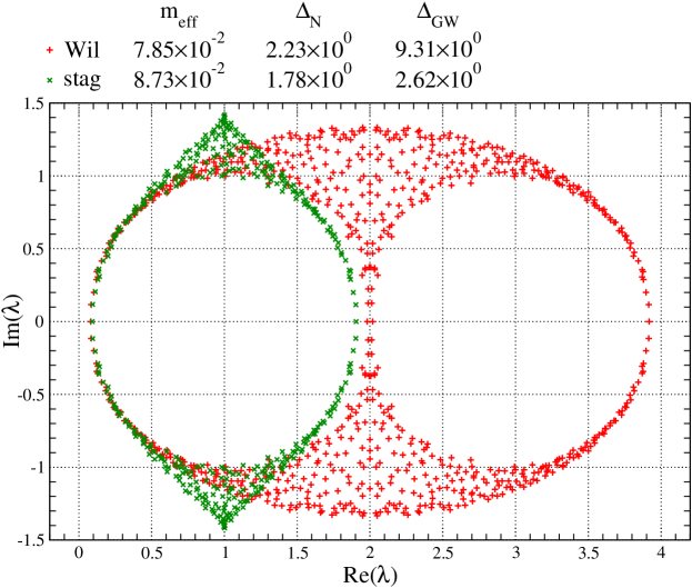
Figure 8: Spectrum of kernel operators in a $\mathrm{U}\!\left(1\right)$ background field.

An example of a kernel eigenvalue spectrum on a gauge configuration with topological charge $Q=1$ can be found in Fig. 8. Compared to the case of four-dimensional quantum chromodynamics, the branches are much sharper and better separated, cf. Chapter 6 and Refs. [70, 71, 82, 4, 7, 8].

Bulk operators.

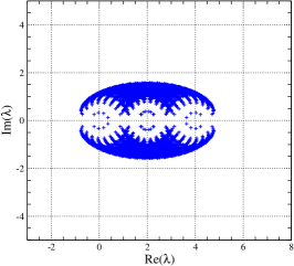
(a) Standard construction

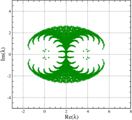
(b) Boriçi’s construction

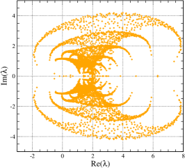
(c) Optimal construction

Figure 9: Spectrum of $D_{\mathsf{dw}}$ with Wilson kernel for $m=0$ at $N_{s}=8$.

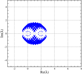
(a) Standard construction

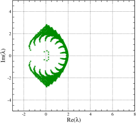
(b) Boriçi’s construction

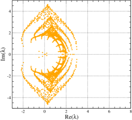
(c) Optimal construction

Figure 10: Spectrum of $D_{\mathsf{sdw}}$ with staggered Wilson kernel for $m=0$ at $N_{s}=8$.

For the eigenvalue spectra of the bulk operators in Figs. 9 and 10 we use the same gauge background field as in Fig. 8. Being a topologically nontrivial configuration, the effective operator has $\left|Q\right|$ approximate zero modes which become exact in the limit $N_{s}\to\infty$. For the bulk operators, there are $N_{s}\cdot\left|Q\right|$ eigenvalues in the neighborhood of the origin. It is an interesting observation to see how the eigenvalue spectrum is distorted in the optimal construction in order to improve chiral properties.

Effective operators.

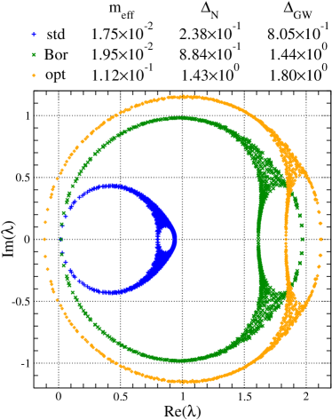
(a) Wilson kernel

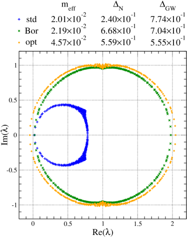
(b) Staggered Wilson kernel

Figure 11: Spectrum of $\varrho D_{\mathsf{eff}}$ for the standard (std), Boriçi (Bor) and optimal (opt) construction at $N_{s}=2$.

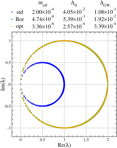
(a) Wilson kernel

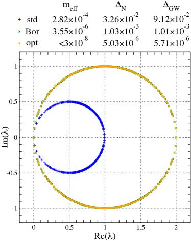
(b) Staggered Wilson kernel

Figure 12: Spectrum of $\varrho D_{\mathsf{eff}}$ for the standard (std), Boriçi (Bor) and optimal (opt) construction at $N_{s}=8$.

Again using the same gauge configuration, in Figs. 11 and 12 we find the eigenvalue spectra of the effective operators. Here Boriçi’s construction shows superior chiral properties compared to the standard construction for $N_{s}\geq 4$ with respect to our measures $m_{\mathsf{eff}}$, $\Delta_{\mathsf{N}}$ and $\Delta_{\mathsf{GW}}$.

The optimal construction further improves upon that and shows an ever lower degree of chiral symmetry violations. In the case of Fig. 12b, the effective mass $m_{\mathsf{eff}}$ is already so small that it is in the order of the round-off error and, thus, we are only able to quote an upper bound. In this nontrivial background field the kernel operators lose their normality and the maximum deviation $\delta_{\mathsf{max}}$ of eigenvalues from the Ginsparg-Wilson circle in the optimal construction does not have to be saturated. We also note that a smaller $\delta_{\mathsf{max}}$ does not necessarily imply a smaller value of $\Delta_{\mathsf{GW}}$, but that also the distribution of eigenvalues of $H$ is important. There is, however, a strong correlation between larger $N_{s}$ and smaller values of $\Delta_{\mathsf{GW}}$, where the violations of the Ginsparg-Wilson relation rapidly tend to zero for $N_{s}\to\infty$.

Chiu’s construction is only in a very particular sense optimal, namely the minimization of the deviation $\delta_{\mathsf{max}}$ from the $\operatorname{sign}$-function as defined in Eq. (3). With respect to other criteria, such as the number of iterations required for solving a linear system, optimal domain wall fermions are typically not optimal [189]. In theory, it is possible to formulate variants of domain wall fermions which are optimal with respect to other measures such as $\Delta_{\mathsf{GW}}$. However, such a construction would likely require more knowledge about the eigenvalue spectrum of $H$.

For the standard construction $m_{\mathsf{eff}}$, $\Delta_{\mathsf{N}}$ and $\Delta_{\mathsf{GW}}$ have typically the same order of magnitude for both a Wilson and a staggered Wilson kernel. On the other hand, for Boriçi’s and the optimal construction a staggered Wilson kernel results in reduced chiral symmetry violations compared to the Wilson kernel.

An interesting, although rather artificial case is $N_{s}=2$. Here we observe that the performance of all constructions is comparable in the case of a staggered Wilson kernel, while for the case of a Wilson kernel the standard construction performs better than Boriçi’s, which itself clearly outperforms the optimal construction.

Overlap operators.

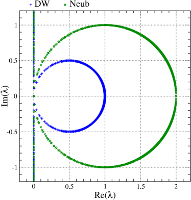
(a) Wilson kernel

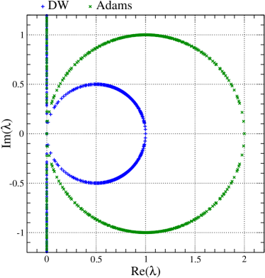
(b) Staggered Wilson kernel

Figure 13: Spectrum of $\varrho D_{\mathsf{ov}}$ with its stereographic projection for the domain wall (DW) kernel and the standard overlap (Neub/Adams) kernel.

In Fig. 13, we again show the spectrum of the associated overlap operators together with a stereographic projection of their eigenvalues. We omit the chirality measures $m_{\mathsf{eff}}$, $\Delta_{\mathsf{N}}$ and $\Delta_{\mathsf{GW}}$ in the figure labels as they vanish up to round-off errors.

3 Smearing

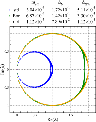
(a) No smearing

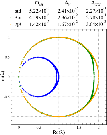
(b) Three smearing iterations

Figure 14: Spectrum of $\varrho D_{\mathsf{eff}}$ with Wilson kernel for the standard (std), Boriçi (Bor) and optimal (opt) construction at $N_{s}=4$ on a smeared configuration with $\alpha=0.5$.

(a) No smearing

(b) Three smearing iterations

Figure 15: Spectrum of $\varrho D_{\mathsf{eff}}$ with staggered Wilson kernel for the standard (std), Boriçi (Bor) and optimal (opt) construction at $N_{s}=4$ on a smeared configuration with $\alpha=0.5$.

Smearing is a common technique in the simulations of lattice gauge theories. It is expected to be especially beneficial for the staggered Wilson kernel (in particular in $3+1$ dimensions) as discussed in Ref. [82]. For this reason we consider gauge fields with three-step ape smearing [216, 217]. For the smearing parameter, we choose the maximal value $\alpha=0.5$ in two dimensions within the perturbatively reasonable range [218].

To test the effects of smearing on the violations of chiral symmetry, in Figs. 14 and 15 we directly compare the effective operators on an unsmeared and smeared version of a gauge configuration at $N_{s}=4$. We observe that after three smearing steps, chiral symmetry violations as measured by $m_{\mathsf{eff}}$, $\Delta_{\mathsf{N}}$ and $\Delta_{\mathsf{GW}}$ are reduced significantly. In some cases we observe a reduction by up to two order of magnitude with the exception of the effective mass for the standard construction with a Wilson kernel.

4 Topology

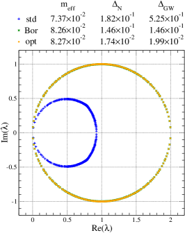
(a) Configuration with $Q=0$

(b) Configuration with $Q=1$

(c) Configuration with $Q=3$

Figure 16: Spectrum of $\varrho D_{\mathsf{eff}}$ with staggered Wilson kernel for the standard (std), Boriçi (Bor) and optimal (opt) construction at $N_{s}=4$ on configurations with various $Q$.

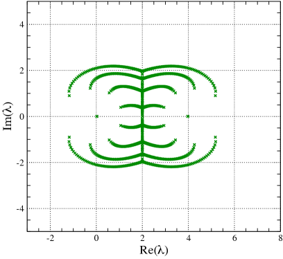
(a) Wilson kernel

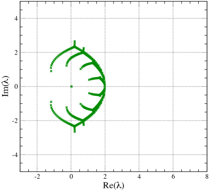
(b) Staggered Wilson kernel

Figure 17: Spectrum of $D_{\mathsf{dw}}$ in Boriçi’s construction at $N_{s}=4$ on a smooth topological configuration with $Q=3$.

On topologically nontrivial configurations with $Q\neq 0$, the Atiyah-Singer index theorem ensures that the continuum Dirac operator has exact zero modes. On the lattice the same can be shown for the overlap operator, while for the effective Dirac operators we only find approximate zero modes as illustrated in Fig. 16. These modes come with a multiplicity of $\left|Q\right|$ as expected from the Vanishing Theorem.

By using the technique outlined in Ref. [211] for constructing a smooth configuration for any given topological charge $Q$, we can study topological aspects also in a more abstract setting. The gauge configurations are maximally smooth in the sense that they are invariant under the application of the ape smearing prescription. We measure $m_{\mathsf{eff}}$, $\Delta_{\mathsf{N}}$ and $\Delta_{\mathsf{GW}}$ for the effective Dirac operators on a wide range of smooth topological configurations with various $Q$. Our measures of chirality are identical for the configurations with $\pm Q$ and only depend on $\left|Q\right|$.

Due to the smoothness of the configurations, the measures $m_{\mathsf{eff}}$, $\Delta_{\mathsf{N}}$ and $\Delta_{\mathsf{GW}}$ are all small compared to the typical values one measures on thermalized configurations at reasonable values of $\beta$. We also observe that with increasing values of $\left|Q\right|$ the chiral symmetry violations become larger. Finally, we show two eigenvalue spectra of bulk operators on a $20^{2}$ lattice in Fig. 17, revealing a very clear structure of the spectrum on a topologically nontrivial configuration.

5 Spectral flow

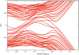
(a) Unsmeared configuration

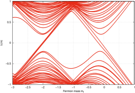
(b) Smeared configuration

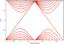
(c) Topological configuration

Figure 18: Spectral flow of the Wilson kernel for configurations with $Q=2$.

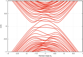
(a) Unsmeared configuration

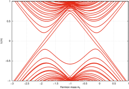
(b) Smeared configuration

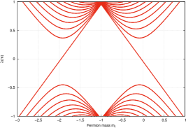
(c) Topological configuration

Figure 19: Spectral flow of the staggered Wilson kernel for configurations with $Q=2$.

Besides the study of the eigenvalue spectra, topological aspects—such as the index theorem—can be studied on the lattice also with the help of spectral flows [219, 105].

Commonly used with a Wilson kernel, one studies the eigenvalues $\lambda\left(m_{\mathsf{f}}\right)$ of the Hermitian operator $H_{\mathsf{w}}\left(m_{\mathsf{f}}\right)$ as a function of $m_{\mathsf{f}}$. One finds a direct one-to-one correspondence between the eigenvalue crossings of $H_{\mathsf{w}}\left(m_{\mathsf{f}}\right)$ and the real eigenvalues of $D_{\mathsf{w}}\left(m_{\mathsf{f}}\right)$. Moreover, the low-lying real eigenvalues of the Wilson Dirac operator $D_{\mathsf{w}}\left(m_{\mathsf{f}}\right)$ correspond to the would-be zero modes [211]. For each respective mode, the slope of the eigenvalue crossings at small values of $m_{\mathsf{f}}$ equals minus its chirality. By studying the eigenvalue crossings of the Hermitian operator in a background field we can, thus, determine the respective topological charge.

Although originally spectral flows of Wilson-like kernels were studied, Adams’ generalized the method to staggered kernels [44] allowing the study of topological aspects within the staggered framework [70, 220, 71, 210]. While in the literature these spectral flows have been investigated before, here we want to show the effectiveness of smearing when studying topological aspects on the lattice.

To this end we show an example for the flow $\lambda\left(m_{\mathsf{f}}\right)$ of the lowest $50$ eigenvalues for the Wilson kernel $H_{\mathsf{w}}\left(m_{\mathsf{f}}\right)$ and the staggered Wilson kernel $H_{\mathsf{sw}}\left(m_{\mathsf{f}}\right)$ in Figs. 18 and 19. The $12^{2}$ gauge configuration under consideration was generated at $\beta=1.8$ and has a topological charge of $Q=2$. We compare the eigenvalue flow on both the unsmeared and the three-step ape smeared ($\alpha=0.5$) version of the configuration and also added the smooth $Q=2$ topological configuration described in Sec. 4. While the determination of the topological charge $Q$ via the spectral flow is not easily possible for the rough and unsmeared configuration, the use of smearing allows an unambiguous identification of the topological sector. In the case of the smooth topological configuration, the two eigenvalue crossings lie essentially on top of each other. The direct comparison between the figures shows the effectiveness of smearing for the study of topological aspects on the lattice.

6 Approaching the continuum

Kernel	Construction	$N_{s}$	$m_{\mathsf{eff}}$	$\Delta_{\mathsf{N}}$	$\Delta_{\mathsf{GW}}$
		2	$5.47\times 10^{-3}$	$1.53\times 10^{-1}$	$6.72\times 10^{-1}$
	Standard	4	$5.90\times 10^{-4}$	$6.87\times 10^{-2}$	$3.10\times 10^{-1}$
		6	$1.00\times 10^{-4}$	$2.30\times 10^{-2}$	$1.02\times 10^{-1}$
		2	$5.73\times 10^{-3}$	$3.71\times 10^{-1}$	$1.16\times 10^{0\phantom{-}}$
Wilson	Boriçi	4	$8.56\times 10^{-5}$	$6.64\times 10^{-2}$	$3.00\times 10^{-1}$
		6	$5.42\times 10^{-6}$	$1.57\times 10^{-2}$	$7.60\times 10^{-2}$
		2	$8.30\times 10^{-3}$	$7.51\times 10^{-1}$	$1.16\times 10^{0\phantom{-}}$
	Optimal	4	$2.11\times 10^{-3}$	$3.59\times 10^{-2}$	$4.78\times 10^{-2}$
		6	$8.71\times 10^{-6}$	$1.21\times 10^{-3}$	$1.74\times 10^{-3}$
		2	$6.22\times 10^{-3}$	$1.48\times 10^{-1}$	$6.49\times 10^{-1}$
	Standard	4	$7.18\times 10^{-4}$	$5.88\times 10^{-2}$	$2.88\times 10^{-1}$
		6	$1.34\times 10^{-4}$	$2.01\times 10^{-2}$	$9.72\times 10^{-2}$
		2	$6.38\times 10^{-3}$	$2.02\times 10^{-1}$	$2.92\times 10^{-1}$
Staggered Wilson	Boriçi	4	$5.13\times 10^{-5}$	$5.45\times 10^{-3}$	$8.68\times 10^{-3}$
		6	$5.91\times 10^{-7}$	$1.53\times 10^{-4}$	$2.69\times 10^{-4}$
		2	$1.72\times 10^{-2}$	$2.32\times 10^{-1}$	$2.66\times 10^{-1}$
	Optimal	4	$3.35\times 10^{-5}$	$2.23\times 10^{-3}$	$2.63\times 10^{-3}$
		6	$5.02\times 10^{-8}$	$2.01\times 10^{-5}$	$2.36\times 10^{-5}$

Table 1: Median values for the various measures of chirality on unsmeared $32^{2}$ configurations generated at $\beta=12.8$. For $m_{\mathsf{eff}}$ only configurations with $Q\neq 0$ are considered.

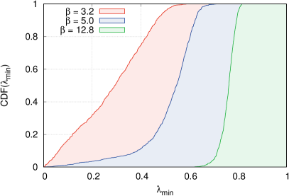
(a) Wilson kernel

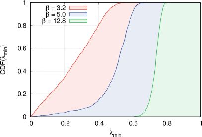
(b) Staggered Wilson kernel

Figure 20: Cumulative distribution function $\mathsf{CDF}$ of $\lambda_{\mathsf{min}}$ for the Hermitian kernel operators.

To evaluate the chiral properties of the various effective Dirac operators when approaching the continuum, we evaluated them on seven ensembles with $1000$ configurations each. While keeping the physical volume fixed, we consider the following ensembles: $8^{2}$ at $\beta=0.8$, $12^{2}$ at $\beta=1.8$, $16^{2}$ at $\beta=3.2$, $20^{2}$ at $\beta=5.0$, $24^{2}$ at $\beta=7.2$, $28^{2}$ at $\beta=9.8$ and $32^{2}$ at $\beta=12.8$. Besides the unsmeared configurations, we also consider the smeared versions, resulting in $N=14\,000$ gauge configurations in total.

While we are interested in the comparison of the different formulations on finer lattices, we do not attempt a rigorous continuum limit analysis. The chirality measures on our finest lattice at $\beta=12.8$ serve us as an indicator for the relative performance of the different domain wall formulations. In Table 1, we quote the median values for the parameter range $N_{s}\in\left\{2,4,6\right\}$. For $N_{s}\geq 8$ some values already become so small, that they are comparable with the round-off error and, thus, cannot be considered reliable. For the standard construction we find that the chiral symmetry violations at large values of $\beta$ are comparable for the cases of a Wilson and a staggered Wilson kernel. At the same time, in the case of Boriçi’s and the optimal construction we often find differences between the two kernel operators of one to two orders of magnitude.

In practical applications the spectral bounds $\lambda_{\mathsf{min}}$ and $\lambda_{\mathsf{max}}$ of optimal domain wall fermions are set on a per ensemble basis. As especially for small $\beta$ and large ensembles one frequently observes values of $\lambda_{\mathsf{min}}$ close to zero, one typically projects out the lowest lying eigenvalues and treats them exactly in order to arrive at a kernel operator with a narrower spectrum. As in our study we want to compare the “baseline performance” of the various domain wall fermion formulations, we decided to not add such an additional algorithmic component mixing into the results of our benchmarks. However, as we also investigate large ensembles at small $\beta$, the observed ratios of $\lambda_{\min}^{2}/\lambda_{\min}^{2}$ can be very small in these cases, rendering the optimal $L_{\infty}$-approximation of the $\operatorname{sign}$-function inadequate and of no practical use. To mitigate this phenomenon, we decided to construct the $\operatorname{sign}$-function approximation on a per-configuration rather than a per-ensemble basis. This means that a small eigenvalue on a given configuration does not render the $\operatorname{sign}$-function approximation inadequate for the whole ensemble, but only on that particular configuration. On the other hand this implies that in our benchmarks the performance of optimal domain wall fermions tend to be overestimated and can only be considered indicative of the performance of Chiu’s formulation of domain wall fermions.

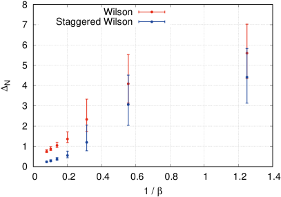
(a) Without smearing

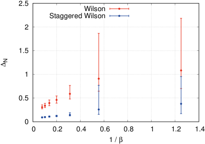
(b) With smearing

Figure 21: Violation of normality $\Delta_{\mathsf{N}}$ as a function of $1/\beta$ for $\varrho D_{\mathsf{eff}}$ in the optimal construction at $N_{s}=2$ (this figure is not part of Ref. [2]).

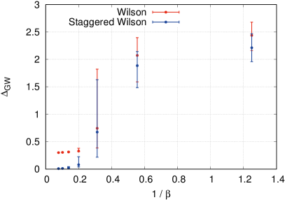
(a) Without smearing

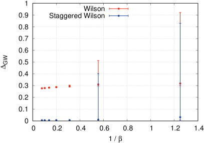
(b) With smearing

Figure 22: Violation of the Ginsparg-Wilson relation $\Delta_{\mathsf{GW}}$ as a function of $1/\beta$ for $\varrho D_{\mathsf{eff}}$ in Boriçi’s construction at $N_{s}=4$.

In general, we find that the standard construction is outperformed by Boriçi’s construction with respect to our chirality measures, while optimal domain wall fermions show the best overall performance. A notable exception is the effective mass $m_{\mathsf{eff}}$, where the optimal construction with a Wilson kernel is not so clearly outperforming the competing variants. This is not surprising, considering that the optimal rational function approximation of the $\operatorname{sign}$-function deviates the most at $\lambda_{\mathsf{min}}$ (and $\lambda_{\mathsf{max}}$) and, thus, low-lying eigenvalues are typically not mapped very accurately. However, as the size of the error decreases rapidly with increasing values of $N_{s}$, this problem is only present for small values of $N_{s}$.

In this context the distribution of the lowest eigenvalue

$$\lambda_{\mathsf{min}}=\min_{\lambda\in\operatorname{spec}H}\left|\lambda\right|$$ (5)

of the respective kernel operators $H=H_{\mathsf{w}}$ and $H=H_{\mathsf{sw}}$ is of interest. In Fig. 20, we show the numerically determined cumulative distribution functions (CDFs) of $\lambda_{\mathsf{min}}$ for both the Wilson and staggered Wilson kernel at different values of $\beta$. When increasing $\beta$, we observe how the distribution moves toward larger values of $\lambda_{\mathsf{min}}$ and pathologically small values become extremely unlikely. This is important, as rational approximations to the $\operatorname{sign}$-function become inaccurate for small arguments. We also note that the corresponding CDFs for the Wilson and staggered Wilson kernel are very similar.

Finally, in Figs. 21 and 22 we show two examples of the $\beta$-dependence of our chiral symmetry measures $\Delta_{\mathsf{N}}$ and $\Delta_{\mathsf{GW}}$. In the plot we show the median value and the width of the distribution. Fixing the value

$$q=\frac{1}{2}\left[1-\operatorname{erf}\left(\frac{1}{\sqrt{2}}\right)\right],$$ (6)

where $\operatorname{erf}\left(x\right)$ refers to the error function, then we define the width using the $q$-quantile and the $\left(1-q\right)$-quantile. With our choice of $q$, we find $68.3\,\mathrm{\%}$ of the values within the range. Our figures illustrate the superior chiral properties of the effective operator with a staggered Wilson kernel at sufficiently large values of $\beta$. With the use of smearing, the chiral properties are even further improved.

7 Quenched quantum chromodynamics

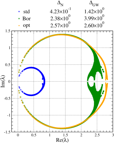
(a) Wilson kernel

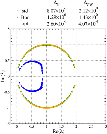
(b) Staggered Wilson kernel

Figure 1: Spectrum of $\varrho D_{\mathsf{eff}}$ at $N_{s}=4$ on a smeared $6^{4}$ configuration in QCD₄ at $\beta=6$.

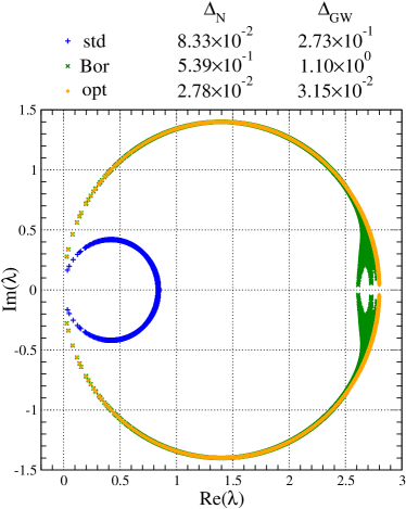
(a) Wilson kernel

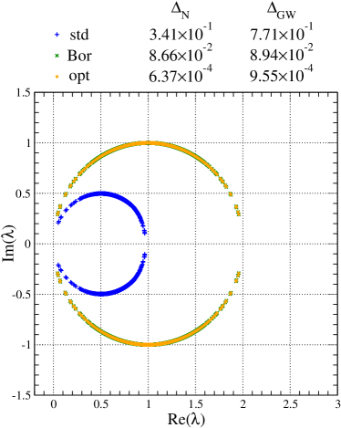
(b) Staggered Wilson kernel

Figure 2: Spectrum of $\varrho D_{\mathsf{eff}}$ at $N_{s}=8$ on a smeared $6^{4}$ configuration in QCD₄ at $\beta=6$.

Although our study focuses on the setting of the Schwinger model, we also investigated the case of four-dimensional quantum chromodynamics. Our results presented here are exploratory in nature, go beyond our discussion in Ref. [2] and were first presented in Ref. [1].

In Figs. 1 and 2 we can find the eigenvalue spectrum of the effective Dirac operator in the standard, Boriçi’s and the optimal construction at $N_{s}\in\left\{4,8\right\}$ on a smeared four-dimensional $6^{4}$ lattice. The $\mathrm{SU}\!\left(3\right)$ gauge configuration under consideration was generated at $\beta=6$ and then smeared with one step of the ape smearing prescription using a smearing parameter of $\alpha=0.65$. As it is a topologically trivial configuration, the effective mass $m_{\mathsf{eff}}$ is omitted in the figure labels. Taking smearing into account, for the domain wall height we use $M_{0}=1.4$ in the case of the Wilson kernel and $M_{0}=1$ for the staggered Wilson kernel.

While in the case of the standard construction with a Wilson kernel we actually observe smaller chiral symmetry violations compared to the staggered Wilson kernel, for Boriçi’s and the optimal construction the use of the staggered Wilson kernel results in clearly superior chiral properties. We often observe a reduction in $\Delta_{\mathsf{N}}$ and $\Delta_{\mathsf{GW}}$ by more than an order of magnitude.

Although without considering more samples it is too early to judge the potential benefits of using staggered domain wall fermions in the setting of four-dimensional quantum chromodynamics, our first results are very encouraging.

8 Optimal weights

$s$	$\omega_{s}\left(\lambda_{\mathsf{min}}=1,\lambda_{\mathsf{max}}=3\right)$	$\omega_{s}\left(\lambda_{\mathsf{min}}=1,\lambda_{\mathsf{max}}=\sqrt{2}\right)$
1	0.989011284192743	0.996659816028010
2	0.908522120246430	0.971110743060917
3	0.779520722603956	0.925723982088869
4	0.641124364053574	0.869740043520870
5	0.519919928211430	0.813009342796322
6	0.427613177773962	0.763841917102527
7	0.366896221792507	0.728142270322088
8	0.337036936444470	0.709476563432225

Table 1: Weight factors $\omega_{s}$ for the optimal domain wall fermion construction.

Before ending this chapter with our conclusions, we quote some example weight factors $\omega_{s}$ for optimal domain wall fermions as defined in Sec. 3. We consider the free-field case in two dimensions and set $M_{0}=1$ and $N_{s}=8$. In the case of the Wilson kernel we then fix $\lambda_{\mathsf{min}}=1$ and $\lambda_{\mathsf{max}}=3$, while for the staggered Wilson kernel we let $\lambda_{\mathsf{min}}=1$ and $\lambda_{\mathsf{max}}=\sqrt{2}$. The resulting weights $\omega_{s}$ can be found in Table 1.

9 Conclusions

In this chapter, we explicitly constructed various formulations of staggered domain wall fermions. We investigated their chiral properties in the free-field case, on quenched thermalized background fields in the Schwinger model and on smooth topological configurations. With respect to our study, staggered domain wall fermions work as advertised and generalize the domain wall fermion construction to staggered kernels.

We also went beyond Adams’ original proposal of staggered domain wall fermions and generalized existing variants to the staggered case, such as Boriçi’s and Chiu’s construction. This resulted in the formulation of truncated staggered domain wall fermions and optimal staggered domain wall fermions, which were previously not considered in the literature. Especially these new variants of staggered domain wall fermions show significantly improved chiral properties compared to the traditional Wilson-based constructions, at least in the context of the Schwinger model. In a setting where chiral symmetry plays an important role, the use of these novel lattice fermion formulations can be potentially very advantageous.

While our results in the setting of a $\mathrm{U}\!\left(1\right)$ gauge theory are very encouraging, the case of a $\mathrm{SU}\!\left(3\right)$ gauge group is not fully understood yet. As our first results in four-dimensional quantum chromodynamics are promising, they warrant further investigations.

Chapter 8 Conclusions

In this thesis we aimed for a better understanding of the theoretical foundations, computational properties and the practical applications of staggered Wilson, staggered domain wall and staggered overlap fermions.

1 Summary

To summarize some of the core parts of this thesis we recall that in Chapter 2, we gave an extensive review of the symmetries of staggered fermions and the construction of flavored mass terms. We discussed both Adams’ proposal for a two-flavor and Hoelbling’s proposal for a one-flavor staggered Wilson term. In Sec. 6, we built upon these ideas and generalized the staggered Wilson term to allow for arbitrary mass splittings in arbitrary even dimensions.

In Chapter 3, we estimated the gains in computational efficiency when using staggered Wilson fermions instead of usual Wilson fermions for inverting the Dirac matrix on a source, where we found a speedup factor of $4\text{--}6$ in our particular benchmark setting. We also analyzed the memory bandwidth requirements of staggered Wilson fermions, quantified by the arithmetic intensity, and found that they are comparable to other common staggered formulations.

In Chapter 4, we demonstrated the feasibility of spectroscopy calculations with staggered Wilson fermions by studying the case of pseudoscalar mesons. We adapted the operators used for spectroscopy with usual staggered fermions and did a numerical study of the pion spectrum when turning the two-flavor staggered Wilson term on.

In Chapter 5, we reviewed the overlap construction and discussed Adams’ generalization to the case of a staggered kernel. In this context we did an analytical verification of the correctness of the continuum limit of the index and axial anomaly for the staggered overlap Dirac operator in Sec. 4.

In Chapter 6, we analyzed the eigenvalue spectrum of the staggered Wilson Dirac operator and related it to the computational efficiency of staggered overlap fermions. We proposed an explanation to resolve the apparent discrepancies in the speedup factors for the staggered Wilson kernel and for the staggered overlap formulation.

Finally, in Chapter 7 we studied Adams’ proposal of staggered domain wall fermions. In the process we generalized some variants of domain wall fermions to a staggered kernel, investigated spectral properties and quantified chiral symmetry violations of various domain wall formulations. We found that in the setting of the Schwinger model the use of a staggered Wilson kernel results in significantly improved chiral properties.

2 Outlook

While staggered Wilson fermions and their derived formulations have both advantages and disadvantages compared to more established lattice fermion formulations, we believe that their use can be beneficial in some settings. In four dimensions, the two flavors of Adams’ staggered Wilson fermions can be naturally used as a discretization of the light up and down quarks. Moreover, compared to Wilson fermions, staggered Wilson fermions are at no disadvantage with respect to flavor-singlet physics [4]. Possible applications include the high precision determination of the $\eta^{\prime}$ mass and the calculation of bulk quantities in thermodynamics [4, 9]. Furthermore, one can test universality, i.e. the independence of physical results of the choice of the lattice action, with the help of new lattice fermion formulations.

While the staggered Wilson kernel defines an interesting lattice fermion discretization in its own right, its derived chiral fermion formulations bear the potential of reducing the computational costs of simulations with chiral lattice fermions significantly. While staggered overlap fermions obey an exact chiral symmetry, staggered domain wall fermions implement an approximate chiral symmetry in a controlled manner. While the achievable speedup factor of staggered overlap fermions compared to Neuberger’s overlap fermions has yet to be determined in a realistic setting (cf. Chapter 6), for staggered domain wall fermions an improvement of chirality by often more than an order of magnitude could be already shown in the Schwinger model.

Besides Adams’ formulation, one may also ask about the potential of Hoelbling’s single flavor staggered action (see Sec. 5). As already pointed out in Ref. [46], it is important to note that in this case the hypercubic rotational symmetry is broken, although the double rotation symmetry is preserved. This results in the need for two gluonic counterterms to restore rotational invariance in unquenched simulations [69] as the terms $G_{12}^{2}+G_{34}^{2}$, $G_{13}^{2}+G_{24}^{2}$ and $G_{14}^{2}+G_{23}^{2}$ can all appear with different coefficients, where $G_{\mu\nu}$ denotes the clover version of the gauge field-strength tensor (see e.g. Ref. [16]).

While this fine-tuning is in principle possible, the simultaneous fine-tuning of coefficients requires significant effort and makes the use of this action unlikely in the context of practical applications in the near future. Perturbative methods allow studying this fine-tuning on an analytical level, although we expect the necessary calculations to quickly become tedious due to the nontrivial structure of terms of the form $G_{\alpha\beta}^{2}+G_{\gamma\delta}^{2}$ with $\alpha$, $\beta$, $\gamma$, $\delta$ pairwise different. While these issues do not render Hoelbling’s formulation invalid, one can get an idea of the challenges ahead from the many-year efforts needed in studying similar issues in the context of minimally doubled fermions of the Karsten-Wilczek kind [221, 222], both on an analytical [223] and a numerical level [224].

For the future, we hope that the practical potential of these new novel fermion formulations is explored further, also in the case of full dynamical simulations. As the technical properties of staggered Wilson fermions mimic the ones of Wilson fermions (with the substitution $D_{\mathsf{w}}\to D_{\mathsf{sw}}$ and $\gamma_{5}\to\epsilon$), it is expected that the commonly employed algorithms for Wilson fermions can be adapted to staggered Wilson fermions.

In particular rational and polynomial hybrid Monte Carlo methods [225, 226, 227] would then allow the generation of two-flavor full QCD configurations and render any rooting procedure—together with any potential related problems—unnecessary. However, practical implementations of these algorithms together with in-depth studies of their theoretical and computational properties are still outstanding and left for future work.

References

- [1] C. Hoelbling and C. Zielinski, “Staggered domain wall fermions,” PoS LATTICE2016 (2016) 254, arXiv:1609.05114 [hep-lat].
- [2] C. Hoelbling and C. Zielinski, “Spectral properties and chiral symmetry violations of (staggered) domain wall fermions in the Schwinger model,” Phys. Rev. D94 no. 1, (2016) 014501, arXiv:1602.08432 [hep-lat].
- [3] D. H. Adams, R. Har, Y. Jia, and C. Zielinski, “Continuum limit of the axial anomaly and index for the staggered overlap Dirac operator: An overview,” PoS LATTICE2013 (2014) 462, arXiv:1312.7230 [hep-lat].
- [4] D. H. Adams, D. Nogradi, A. Petrashyk, and C. Zielinski, “Computational efficiency of staggered Wilson fermions: A first look,” PoS LATTICE2013 (2014) 353, arXiv:1312.3265 [hep-lat].
- [5] K. G. Wilson, “Confinement of quarks,” Phys. Rev. D10 (1974) 2445–2459.
- [6] K. G. Wilson, “Quarks and strings on a lattice,” in New Phenomena in Subnuclear Physics: Part A, A. Zichichi, ed., pp. 69–142. Springer US, Boston, MA, 1977. Proceedings of the First Half of the International School of Subnuclear Physics, Erice, Sicily, July 11 – August 1, 1975.
- [7] C. Zielinski, “Computational Efficiency and Spectrum Results for Staggered Wilson Fermions.” Talk given at the 32nd International Symposium on Lattice Field Theory, New York City, USA, 2014.
- [8] C. Zielinski, “More Results on the Computational Efficiency of Staggered Wilson Fermions.” Talk given at the 9th International Conference on Computational Physics, Singapore, Singapore, 2015.
- [9] D. H. Adams, “Update on staggered Wilson fermions.” Talk given at the 32nd International Symposium on Lattice Field Theory, New York City, USA, 2014.
- [10] C. Zielinski, “Pion spectrum for the 2-flavor staggered Wilson fermion.” Talk given at the 33rd International Symposium on Lattice Field Theory, Kobe, Japan, 2015.
- [11] R. Har, Index of lattice Dirac operators. PhD thesis, Nanyang Technological University, 2014. {https://dr.ntu.edu.sg/handle/10356/61803}.
- [12] C. Zielinski, “On the Eigenvalue Spectrum of (Staggered) Domain Wall Fermions.” Talk given at the Spring Meeting of the German Physical Society, Hamburg, Germany, 2016.
- [13] S. Weinberg, The Quantum theory of fields. Vol. 1: Foundations. Cambridge University Press, 2005.
- [14] S. Weinberg, The quantum theory of fields. Vol. 2: Modern applications. Cambridge University Press, 2013.
- [15] M. E. Peskin and D. V. Schroeder, An introduction to quantum field theory. Advanced book program. Westview Press Reading, 1995.
- [16] C. Gattringer and C. Lang, Quantum Chromodynamics on the Lattice: An Introductory Presentation. Lecture Notes in Physics. Springer Berlin Heidelberg, 2009.
- [17] T. DeGrand and C. DeTar, Lattice Methods for Quantum Chromodynamics. World Scientific, 2006.
- [18] I. Montvay and G. Munster, Quantum fields on a lattice. Cambridge University Press, 1997.
- [19] H. J. Rothe, Lattice Gauge Theories: An Introduction. World Scientific, 2005.
- [20] P. A. M. Dirac, “The quantum theory of the electron,” Proc. Roy. Soc. Lond. A117 (1928) 610–624.
- [21] F. A. Berezin, The method of second quantization. Pure and applied physics. Academic Press, 1966.
- [22] C.-N. Yang and R. L. Mills, “Conservation of Isotopic Spin and Isotopic Gauge Invariance,” Phys. Rev. 96 (1954) 191–195.
- [23] R. P. Feynman, “Space-time approach to nonrelativistic quantum mechanics,” Rev. Mod. Phys. 20 (1948) 367–387.
- [24] R. P. Feynman, “Space-time approach to quantum electrodynamics,” Phys. Rev. 76 (1949) 769–789.
- [25] S. Albeverio, R. Høegh-Krohn, and S. Mazzucchi, Mathematical Theory of Feynman Path Integrals: An Introduction. Lecture Notes in Mathematics. Springer Berlin Heidelberg, 2008.
- [26] L. D. Faddeev and V. N. Popov, “Feynman Diagrams for the Yang-Mills Field,” Phys. Lett. B25 (1967) 29–30.
- [27] T. Aoyama, M. Hayakawa, T. Kinoshita, and M. Nio, “Tenth-Order QED Contribution to the Electron and an Improved Value of the Fine Structure Constant,” Phys. Rev. Lett. 109 (2012) 111807, arXiv:1205.5368 [hep-ph].
- [28] G. C. Wick, “Properties of Bethe-Salpeter Wave Functions,” Phys. Rev. 96 (1954) 1124–1134.
- [29] N. Sadooghi and H. J. Rothe, “Continuum behavior of lattice QED, discretized with one sided lattice differences, in one loop order,” Phys. Rev. D55 (1997) 6749–6759, arXiv:hep-lat/9610001 [hep-lat].
- [30] H. B. Nielsen and M. Ninomiya, “No Go theorem for regularizing chiral fermions,” Phys. Lett. B105 (1981) 219.
- [31] H. B. Nielsen and M. Ninomiya, “Absence of neutrinos on a lattice: (I). Proof by Homotopy theory,” Nucl. Phys. B185 (1981) 20. Erratum: Nucl. Phys. B195, 541 (1982).
- [32] H. B. Nielsen and M. Ninomiya, “Absence of neutrinos on a lattice: (II). Intuitive topological proof,” Nucl. Phys. B193 (1981) 173.
- [33] D. Friedan, “A proof of the Nielsen-Ninomiya theorem,” Commun. Math. Phys. 85 (1982) 481–490.
- [34] J. B. Kogut and L. Susskind, “Hamiltonian formulation of Wilson’s lattice gauge theories,” Phys.Rev. D11 (1975) 395.
- [35] T. Banks, L. Susskind, and J. B. Kogut, “Strong coupling calculations of lattice gauge theories: (1+1)-dimensional exercises,” Phys.Rev. D13 (1976) 1043.
- [36] Cornell-Oxford-Tel Aviv-Yeshiva Collaboration, T. Banks, S. Raby, L. Susskind, J. Kogut, D. R. T. Jones, P. N. Scharbach, and D. K. Sinclair, “Strong coupling calculations of the hadron spectrum of quantum chromodynamics,” Phys.Rev. D15 (1977) 1111.
- [37] L. Susskind, “Lattice fermions,” Phys.Rev. D16 (1977) 3031–3039.
- [38] H. Kluberg-Stern, A. Morel, O. Napoly, and B. Petersson, “Flavors of Lagrangian Susskind Fermions,” Nucl. Phys. B220 (1983) 447–470.
- [39] F. Gliozzi, “Spinor algebra of the one component lattice fermions,” Nucl. Phys. B204 (1982) 419–428.
- [40] H. S. Sharatchandra, H. J. Thun, and P. Weisz, “Susskind Fermions on a Euclidean Lattice,” Nucl. Phys. B192 (1981) 205–236.
- [41] C. van den Doel and J. Smit, “Dynamical Symmetry Breaking in Two Flavor SU() and SO() Lattice Gauge Theories,” Nucl. Phys. B228 (1983) 122–144.
- [42] M. F. L. Golterman and J. Smit, “Selfenergy and flavor interpretation of staggered fermions,” Nucl. Phys. B245 (1984) 61.
- [43] D. Daniel and T. D. Kieu, “On the Flavor Interpretations of Staggered Fermions,” Phys. Lett. B175 (1986) 73–76.
- [44] D. H. Adams, “Theoretical Foundation for the Index Theorem on the Lattice with Staggered Fermions,” Phys. Rev. Lett. 104 (2010) 141602, arXiv:0912.2850 [hep-lat].
- [45] D. H. Adams, “Pairs of chiral quarks on the lattice from staggered fermions,” Phys. Lett. B699 (2011) 394–397, arXiv:1008.2833 [hep-lat].
- [46] C. Hoelbling, “Single flavor staggered fermions,” Phys. Lett. B696 (2011) 422–425, arXiv:1009.5362 [hep-lat].
- [47] Y. Iwasaki and T. Yoshie, “Renormalization Group Improved Action for SU(3) Lattice Gauge Theory and the String Tension,” Phys. Lett. B143 (1984) 449–452.
- [48] Y. Iwasaki, K. Kanaya, T. Kaneko, and T. Yoshie, “Scaling in SU(3) pure gauge theory with a renormalization group improved action,” Phys. Rev. D56 (1997) 151–160, arXiv:hep-lat/9610023 [hep-lat].
- [49] QCD-TARO Collaboration, P. de Forcrand, M. G. Perez, T. Hashimoto, S. Hioki, H. Matsufuru, O. Miyamura, A. Nakamura, I. O. Stamatescu, T. Takaishi, and T. Umeda, “Renormalization group flow of SU(3) lattice gauge theory: Numerical studies in a two coupling space,” Nucl. Phys. B577 (2000) 263–278, arXiv:hep-lat/9911033 [hep-lat].
- [50] A. Borici and R. Rosenfelder, “Scaling in SU(3) theory with a MCRG improved lattice action,” Nucl. Phys. Proc. Suppl. 63 (1998) 925–927, arXiv:hep-lat/9711035 [hep-lat].
- [51] M. Golterman, Y. Shamir, and B. Svetitsky, “Localization properties of lattice fermions with plaquette and improved gauge actions,” Phys. Rev. D72 (2005) 034501, arXiv:hep-lat/0503037 [hep-lat].
- [52] R. Y. Rubinstein and D. P. Kroese, Simulation and the Monte Carlo method, vol. 707. John Wiley & Sons, 2011.
- [53] G. C. Wick, “The Evaluation of the Collision Matrix,” Phys. Rev. 80 (1950) 268–272.
- [54] K. Jansen, “Lattice QCD: A Critical status report,” PoS LATTICE2008 (2008) 010, arXiv:0810.5634 [hep-lat].
- [55] PACS-CS Collaboration, S. Aoki, N. Ishii, K.-I. Ishikawa, N. Ishizuka, T. Izubuchi, D. Kadoh, K. Kanaya, Y. Kuramashi, Y. Namekawa, O. H. Nguyen, M. Okawa, K. Sasaki, Y. Taniguchi, A. Ukawa, N. Ukita, T. Yamazaki, and T. Yoshié, “Lattice quantum chromodynamics at the physical point and beyond,” PTEP 2012 (2012) 01A102.
- [56] T. Misumi, “New fermion discretizations and their applications,” PoS LATTICE2012 (2012) 005, arXiv:1211.6999 [hep-lat].
- [57] T. Misumi, Research on novel lattice fermions toward efficient QCD simulations. PhD thesis, Kyoto University, 2012.
- [58] D. H. Adams, “On the fourth root prescription for dynamical staggered fermions,” Phys. Rev. D72 (2005) 114512, arXiv:hep-lat/0411030 [hep-lat].
- [59] A. Hasenfratz and R. Hoffmann, “Validity of the rooted staggered determinant in the continuum limit,” Phys. Rev. D74 (2006) 014511, arXiv:hep-lat/0604010 [hep-lat].
- [60] C. Bernard, M. Golterman, Y. Shamir, and S. R. Sharpe, “Comment on ‘Chiral anomalies and rooted staggered fermions’,” Phys. Lett. B649 (2007) 235–240, arXiv:hep-lat/0603027 [hep-lat].
- [61] C. Bernard, M. Golterman, Y. Shamir, and S. R. Sharpe, “’t Hooft vertices, partial quenching, and rooted staggered QCD,” Phys. Rev. D77 (2008) 114504, arXiv:0711.0696 [hep-lat].
- [62] C. Bernard, M. Golterman, Y. Shamir, and S. R. Sharpe, “Reply to: ‘Comment on: ’t Hooft vertices, partial quenching, and rooted staggered QCD’,” Phys. Rev. D78 (2008) 078502, arXiv:0808.2056 [hep-lat].
- [63] D. H. Adams, “The Rooting issue for a lattice fermion formulation similar to staggered fermions but without taste mixing,” Phys. Rev. D77 (2008) 105024, arXiv:0802.3029 [hep-lat].
- [64] M. Creutz, “Chiral anomalies and rooted staggered fermions,” Phys. Lett. B649 (2007) 230–234, arXiv:hep-lat/0701018 [hep-lat].
- [65] M. Creutz, “Reply to: “Comment on: ‘Chiral anomalies and rooted staggered fermions”’,” Phys. Lett. B649 (2007) 241–242, arXiv:0704.2016 [hep-lat].
- [66] M. Creutz, “Comment on ‘ ’t Hooft vertices, partial quenching, and rooted staggered QCD’,” Phys. Rev. D78 (2008) 078501, arXiv:0805.1350 [hep-lat].
- [67] S. R. Sharpe, “Rooted staggered fermions: Good, bad or ugly?,” PoS LAT2006 (2006) 022, arXiv:hep-lat/0610094 [hep-lat].
- [68] M. Golterman, “QCD with rooted staggered fermions,” PoS CONFINEMENT8 (2008) 014, arXiv:0812.3110 [hep-ph].
- [69] S. R. Sharpe, “Comments on non-degenerate staggered fermions, staggered Wilson and Overlap fermions, and the application of chiral perturbation theory to lattice fermions.” Talk given at Yukawa Institute Workshop “New Types of Fermions on the Lattice”, Kyoto, Japan, 2012.
- [70] P. de Forcrand, A. Kurkela, and M. Panero, “Numerical properties of staggered overlap fermions,” PoS LATTICE2010 (2010) 080, arXiv:1102.1000 [hep-lat].
- [71] P. de Forcrand, A. Kurkela, and M. Panero, “Numerical properties of staggered quarks with a taste-dependent mass term,” JHEP 04 (2012) 142, arXiv:1202.1867 [hep-lat].
- [72] S. Aoki, “New Phase Structure for Lattice QCD with Wilson Fermions,” Phys. Rev. D30 (1984) 2653.
- [73] S. Aoki, “The U(1) Problem on a Lattice. 1. Strong Coupling Limit,” Phys. Rev. D33 (1986) 2399.
- [74] S. Aoki, “The U(1) Problem on a Lattice. 2. Strong Coupling Expansion,” Phys. Rev. D34 (1986) 3170.
- [75] S. Aoki, “A Solution to the U(1) Problem on a Lattice,” Phys. Rev. Lett. 57 (1986) 3136.
- [76] S. Aoki, “U(1) Problem and Lattice QCD,” Nucl. Phys. B314 (1989) 79–111.
- [77] M. Creutz, “Wilson fermions at finite temperature,” in RHIC Summer Study 96: Brookhaven Theory Workshop on Relativistic Heavy Ions Upton, New York, July 8-19, 1996. 1996. arXiv:hep-lat/9608024 [hep-lat].
- [78] S. R. Sharpe and R. L. Singleton, Jr, “Spontaneous flavor and parity breaking with Wilson fermions,” Phys. Rev. D58 (1998) 074501, arXiv:hep-lat/9804028 [hep-lat].
- [79] T. Misumi, M. Creutz, T. Kimura, T. Z. Nakano, and A. Ohnishi, “Aoki Phases in Staggered-Wilson Fermions,” PoS LATTICE2011 (2011) 108, arXiv:1110.1231 [hep-lat].
- [80] T. Misumi, T. Z. Nakano, T. Kimura, and A. Ohnishi, “Strong-coupling Analysis of Parity Phase Structure in Staggered-Wilson Fermions,” Phys. Rev. D86 (2012) 034501, arXiv:1205.6545 [hep-lat].
- [81] T. Z. Nakano, T. Misumi, T. Kimura, and A. Ohnishi, “Strong coupling analysis of Aoki phase in Staggered-Wilson fermions,” PoS LATTICE2012 (2012) 203, arXiv:1210.5954 [hep-lat].
- [82] S. Durr, “Taste-split staggered actions: eigenvalues, chiralities and Symanzik improvement,” Phys. Rev. D87 no. 11, (2013) 114501, arXiv:1302.0773 [hep-lat].
- [83] C. Lanczos, “An iteration method for the solution of the eigenvalue problem of linear differential and integral operators,” J. Res. Natl. Bur. Stand. B Math. Sci. 45 (1950) 255–282.
- [84] M. R. Hestenes and E. Stiefel, Methods of conjugate gradients for solving linear systems, vol. 49. NBS, 1952.
- [85] J. R. Shewchuk, “An introduction to the conjugate gradient method without the agonizing pain,” 1994.
- [86] M. G. Alford, T. R. Klassen, and G. P. Lepage, “Improving lattice quark actions,” Nucl. Phys. B496 (1997) 377–407, arXiv:hep-lat/9611010 [hep-lat].
- [87] SciDAC, LHPC, UKQCD Collaboration, R. G. Edwards and B. Joo, “The Chroma software system for lattice QCD,” Nucl. Phys. Proc. Suppl. 140 (2005) 832, arXiv:hep-lat/0409003 [hep-lat].
- [88] D. H. Adams, “New staggered-type fermions on the lattice: a review.” Talk given at Yukawa Institute Workshop “New Types of Fermions on the Lattice”, Kyoto, Japan, 2012.
- [89] M. H. Quenouille, “Problems in plane sampling,” Ann. Math. Statist. 20 no. 3, (1949) 355–375.
- [90] M. H. Quenouille, “Notes on bias in estimation,” Biometrika 43 no. 3-4, (1956) 353–360.
- [91] J. W. Tukey, “Bias and confidence in not-quite large samples,” in Annals of Mathematical statistics, vol. 29, pp. 614–614. 1958.
- [92] J. Jeffers and J. Reinders, High Performance Parallelism Pearls Volume Two: Multicore and Many-core Programming Approaches. Elsevier Science, 2015.
- [93] P. A. Boyle, “The BAGEL assembler generation library,” Comput. Phys. Commun. 180 (2009) 2739–2748.
- [94] R. Brower, “Quarks, GPUs and Multigrid.” Talk given at the summer institute “Scientific Computing in the Americas: the challenge of massive parallelism”, Valparaiso, Chile, 2011.
- [95] M. Wagner, “GPUs Immediately Relating Lattice QCD to Collider Experiments.” Talk given at the “GPU Technology Conference 2013”, San José, USA, 2013.
- [96] HPQCD, UKQCD Collaboration, E. Follana, Q. Mason, C. Davies, K. Hornbostel, G. P. Lepage, J. Shigemitsu, H. Trottier, and K. Wong, “Highly improved staggered quarks on the lattice, with applications to charm physics,” Phys. Rev. D75 (2007) 054502, arXiv:hep-lat/0610092 [hep-lat].
- [97] MILC Collaboration, K. Orginos, D. Toussaint, and R. L. Sugar, “Variants of fattening and flavor symmetry restoration,” Phys. Rev. D60 (1999) 054503, arXiv:hep-lat/9903032 [hep-lat].
- [98] M. F. L. Golterman, “Staggered Mesons,” Nucl. Phys. B273 (1986) 663.
- [99] W.-J. Lee and S. R. Sharpe, “Partial flavor symmetry restoration for chiral staggered fermions,” Phys. Rev. D60 (1999) 114503, arXiv:hep-lat/9905023 [hep-lat].
- [100] T. Bae, D. H. Adams, C. Jung, H.-J. Kim, 2, J. Kim, K. Kim, W. Lee, and S. R. Sharpe, “Taste symmetry breaking with HYP-smeared staggered fermions,” Phys. Rev. D77 (2008) 094508, arXiv:0801.3000 [hep-lat].
- [101] N. Ishizuka, M. Fukugita, H. Mino, M. Okawa, and A. Ukawa, “Operator dependence of hadron masses for Kogut-Susskind quarks on the lattice,” Nucl. Phys. B411 (1994) 875–902.
- [102] R. Narayanan and H. Neuberger, “Infinitely many regulator fields for chiral fermions,” Phys. Lett. B302 (1993) 62–69, arXiv:hep-lat/9212019 [hep-lat].
- [103] R. Narayanan and H. Neuberger, “Chiral fermions on the lattice,” Phys. Rev. Lett. 71 (1993) 3251–3254, arXiv:hep-lat/9308011 [hep-lat].
- [104] R. Narayanan and H. Neuberger, “Chiral determinant as an overlap of two vacua,” Nucl. Phys. B412 (1994) 574–606, arXiv:hep-lat/9307006 [hep-lat].
- [105] R. Narayanan and H. Neuberger, “A construction of lattice chiral gauge theories,” Nucl. Phys. B443 (1995) 305–385, arXiv:hep-th/9411108 [hep-th].
- [106] H. Neuberger, “Exactly massless quarks on the lattice,” Phys. Lett. B417 (1998) 141–144, arXiv:hep-lat/9707022 [hep-lat].
- [107] H. Neuberger, “A Practical Implementation of the Overlap Dirac Operator,” Phys. Rev. Lett. 81 (1998) 4060–4062, arXiv:hep-lat/9806025 [hep-lat].
- [108] H. Neuberger, “More about exactly massless quarks on the lattice,” Phys. Lett. B427 (1998) 353–355, arXiv:hep-lat/9801031 [hep-lat].
- [109] P. H. Ginsparg and K. G. Wilson, “A remnant of chiral symmetry on the lattice,” Phys. Rev. D25 (1982) 2649.
- [110] P. Hasenfratz, V. Laliena, and F. Niedermayer, “The index theorem in QCD with a finite cutoff,” Phys. Lett. B427 (1998) 125–131, arXiv:hep-lat/9801021 [hep-lat].
- [111] M. Luscher, “Exact chiral symmetry on the lattice and the Ginsparg-Wilson relation,” Phys. Lett. B428 (1998) 342–345, arXiv:hep-lat/9802011 [hep-lat].
- [112] D. H. Adams, “Index and overlap construction for staggered fermions,” PoS LATTICE2010 (2010) 073, arXiv:1103.6191 [hep-lat].
- [113] P. Hasenfratz, “Prospects for perfect actions,” Nucl. Phys. Proc. Suppl. 63 (1998) 53–58, arXiv:hep-lat/9709110 [hep-lat].
- [114] I. Horvath, “Ginsparg-Wilson relation and ultralocality,” Phys. Rev. Lett. 81 (1998) 4063–4066, arXiv:hep-lat/9808002 [hep-lat].
- [115] P. Hernandez, K. Jansen, and M. Luscher, “Locality properties of Neuberger’s lattice Dirac operator,” Nucl. Phys. B552 (1999) 363–378, arXiv:hep-lat/9808010 [hep-lat].
- [116] J. van den Eshof, A. Frommer, T. Lippert, K. Schilling, and H. A. van der Vorst, “A Comparative study of numerical methods for the overlap Dirac operator: A Status report,” Nucl. Phys. Proc. Suppl. 106 (2002) 1070–1072, arXiv:hep-lat/0110198 [hep-lat].
- [117] J. van den Eshof, A. Frommer, T. Lippert, K. Schilling, and H. A. van der Vorst, “Numerical methods for the QCD overlap operator. I. Sign function and error bounds,” Comput. Phys. Commun. 146 (2002) 203–224, arXiv:hep-lat/0202025 [hep-lat].
- [118] G. Arnold, N. Cundy, J. van den Eshof, A. Frommer, S. Krieg, T. Lippert, and K. Schafer, “Numerical methods for the QCD overlap operator. 2. Optimal Krylov subspace methods,” arXiv:hep-lat/0311025 [hep-lat].
- [119] N. Cundy, J. van den Eshof, A. Frommer, S. Krieg, T. Lippert, and K. Schafer, “Numerical methods for the QCD overlap operator. 3. Nested iterations,” Comput. Phys. Commun. 165 (2005) 221–242, arXiv:hep-lat/0405003 [hep-lat].
- [120] N. Cundy, S. Krieg, G. Arnold, A. Frommer, T. Lippert, and K. Schilling, “Numerical methods for the QCD overlap operator IV: Hybrid Monte Carlo,” Comput. Phys. Commun. 180 (2009) 26–54, arXiv:hep-lat/0502007 [hep-lat].
- [121] M. F. Atiyah and I. M. Singer, “The index of elliptic operators: I,” Annals of Mathematics 87 no. 3, (1968) 484–530.
- [122] M. F. Atiyah and I. M. Singer, “The index of elliptic operators: III,” Annals of Mathematics 87 no. 3, (1968) 546–604.
- [123] M. F. Atiyah and I. M. Singer, “The index of elliptic operators: IV,” Annals of Mathematics 93 no. 1, (1971) 119–138.
- [124] M. F. Atiyah and I. M. Singer, “The index of elliptic operators: V,” Annals of Mathematics 93 no. 1, (1971) 139–149.
- [125] J. E. Kiskis, “Fermions in a pseudoparticle field,” Phys. Rev. D15 (1977) 2329.
- [126] N. K. Nielsen and B. Schroer, “Axial anomaly and Atiyah-Singer theorem,” Nucl. Phys. B127 (1977) 493.
- [127] M. M. Ansourian, “Index theory and the axial current anomaly in two-dimensions,” Phys. Lett. B70 (1977) 301.
- [128] S. L. Adler, “Axial vector vertex in spinor electrodynamics,” Phys. Rev. 177 (1969) 2426–2438.
- [129] J. S. Bell and R. Jackiw, “A PCAC puzzle: in the -model,” Nuovo Cim. A60 (1969) 47–61.
- [130] K. Fujikawa, “Path Integral Measure for Gauge Invariant Fermion Theories,” Phys. Rev. Lett. 42 (1979) 1195–1198.
- [131] K. Fujikawa, “Path Integral for Gauge Theories with Fermions,” Phys. Rev. D21 (1980) 2848. Erratum: Phys. Rev. D22, 1499 (1980).
- [132] K. Fujikawa, “Comment on Chiral and Conformal Anomalies,” Phys. Rev. Lett. 44 (1980) 1733.
- [133] E. Witten, “Current Algebra Theorems for the U(1) Goldstone Boson,” Nucl. Phys. B156 (1979) 269–283.
- [134] G. Veneziano, “U(1) Without Instantons,” Nucl. Phys. B159 (1979) 213–224.
- [135] G. Veneziano, “Goldstone Mechanism From Gluon Dynamics,” Phys. Lett. B95 (1980) 90–92.
- [136] L. Giusti, G. C. Rossi, M. Testa, and G. Veneziano, “The U(A)(1) problem on the lattice with Ginsparg-Wilson fermions,” Nucl. Phys. B628 (2002) 234–252, arXiv:hep-lat/0108009 [hep-lat].
- [137] E. Seiler, “Some more remarks on the Witten-Veneziano formula for the mass,” Phys. Lett. B525 (2002) 355–359, arXiv:hep-th/0111125 [hep-th].
- [138] L. Giusti, G. C. Rossi, and M. Testa, “Topological susceptibility in full QCD with Ginsparg-Wilson fermions,” Phys. Lett. B587 (2004) 157–166, arXiv:hep-lat/0402027 [hep-lat].
- [139] M. Luscher, “Topological effects in QCD and the problem of short distance singularities,” Phys. Lett. B593 (2004) 296–301, arXiv:hep-th/0404034 [hep-th].
- [140] M. Aguado and E. Seiler, “The Clash of positivities in topological density correlators,” Phys. Rev. D72 (2005) 094502, arXiv:hep-lat/0503015 [hep-lat].
- [141] Y. Kikukawa and A. Yamada, “Weak coupling expansion of massless QCD with a Ginsparg-Wilson fermion and axial U(1) anomaly,” Phys. Lett. B448 (1999) 265–274, arXiv:hep-lat/9806013 [hep-lat].
- [142] K. Fujikawa, “A Continuum limit of the chiral Jacobian in lattice gauge theory,” Nucl. Phys. B546 (1999) 480–494, arXiv:hep-th/9811235 [hep-th].
- [143] H. Suzuki, “Simple evaluation of chiral Jacobian with overlap Dirac operator,” Prog. Theor. Phys. 102 (1999) 141–147, arXiv:hep-th/9812019 [hep-th].
- [144] D. H. Adams, “Axial anomaly and topological charge in lattice gauge theory with overlap Dirac operator,” Annals Phys. 296 (2002) 131–151, arXiv:hep-lat/9812003 [hep-lat].
- [145] D. H. Adams, “On the continuum limit of fermionic topological charge in lattice gauge theory,” J. Math. Phys. 42 (2001) 5522–5533, arXiv:hep-lat/0009026 [hep-lat].
- [146] A. Petrashyk, “Spectral flow of staggered Wilson Dirac operator in SU(2) instanton backgrounds.” Talk given at Yukawa Institute Workshop “New Types of Fermions on the Lattice”, Kyoto, Japan, 2012.
- [147] D. H. Adams and W. Bietenholz, “Axial anomaly and index of the overlap hypercube operator,” Eur. Phys. J. C34 (2004) 245–253, arXiv:hep-lat/0307022 [hep-lat].
- [148] W. Bietenholz, “Solutions of the Ginsparg-Wilson relation and improved domain wall fermions,” Eur. Phys. J. C6 (1999) 537–547, arXiv:hep-lat/9803023 [hep-lat].
- [149] E. Anderson, Z. Bai, C. Bischof, S. Blackford, J. Demmel, J. Dongarra, J. D. Croz, A. Greenbaum, S. Hammarling, A. McKenney, and D. Sorensen, LAPACK Users’ Guide. Philadelphia, third ed., 1999.
- [150] J. G. F. Francis, “The QR Transformation A Unitary Analogue to the LR Transformation–Part 1,” The Computer Journal 4 no. 3, (1961) 265–271.
- [151] J. G. F. Francis, “The QR Transformation–Part 2,” The Computer Journal 4 no. 4, (1962) 332–345.
- [152] V. N. Kublanovskaya, “On some algorithms for the solution of the complete eigenvalue problem,” USSR Computational Mathematics and Mathematical Physics 1 no. 3, (1962) 637–657.
- [153] R. Lehoucq, D. Sorensen, and C. Yang, ARPACK Users’ Guide, 1998.
- [154] R. B. Lehoucq and D. C. Sorensen, “Deflation Techniques for an Implicitly Restarted Arnoldi Iteration,” SIAM Journal on Matrix Analysis and Applications 17 no. 4, (1996) 789–821.
- [155] G. I. Egri, Z. Fodor, S. D. Katz, and K. K. Szabo, “Topology with dynamical overlap fermions,” JHEP 01 (2006) 049, arXiv:hep-lat/0510117 [hep-lat].
- [156] JLQCD Collaboration, H. Fukaya, S. Hashimoto, K.-I. Ishikawa, T. Kaneko, H. Matsufuru, T. Onogi, and N. Yamada, “Lattice gauge action suppressing near-zero modes of ,” Phys. Rev. D74 (2006) 094505, arXiv:hep-lat/0607020 [hep-lat].
- [157] N. Cundy, S. Krieg, T. Lippert, and A. Schafer, “Topological tunneling with dynamical overlap fermions,” Comput. Phys. Commun. 180 (2009) 201–208, arXiv:0803.0294 [hep-lat].
- [158] N. Cundy and W. Lee, “Modifying the molecular dynamics action to increase topological tunnelling rate for dynamical overlap fermions,” arXiv:1110.1948 [hep-lat].
- [159] D. B. Kaplan, “A Method for simulating chiral fermions on the lattice,” Phys. Lett. B288 (1992) 342–347, arXiv:hep-lat/9206013 [hep-lat].
- [160] Y. Shamir, “Chiral fermions from lattice boundaries,” Nucl. Phys. B406 (1993) 90–106, arXiv:hep-lat/9303005 [hep-lat].
- [161] V. Furman and Y. Shamir, “Axial symmetries in lattice QCD with Kaplan fermions,” Nucl. Phys. B439 (1995) 54–78, arXiv:hep-lat/9405004 [hep-lat].
- [162] P. M. Vranas, “Chiral symmetry restoration in the Schwinger model with domain wall fermions,” Phys. Rev. D57 (1998) 1415–1432, arXiv:hep-lat/9705023 [hep-lat].
- [163] S. Aoki and Y. Taniguchi, “One loop calculation in lattice QCD with domain wall quarks,” Phys. Rev. D59 (1999) 054510, arXiv:hep-lat/9711004 [hep-lat].
- [164] Y. Kikukawa, H. Neuberger, and A. Yamada, “Exponential suppression of radiatively induced mass in the truncated overlap,” Nucl. Phys. B526 (1998) 572–596, arXiv:hep-lat/9712022 [hep-lat].
- [165] P. Chen, N. H. Christ, G. T. Fleming, A. Kaehler, C. Malureanu, R. Mawhinney, G. Siegert, C. zhong Sui, Y. Zhestkov, and P. M. Vranas, “Toward the chiral limit of QCD: Quenched and dynamical domain wall fermions,” in High-energy physics. Proceedings, 29th International Conference, ICHEP’98, Vancouver, Canada, July 23-29, 1998. Vol. 1, 2. 1998. arXiv:hep-lat/9812011 [hep-lat].
- [166] T. Blum, “Domain wall fermions in vector gauge theories,” Nucl. Phys. Proc. Suppl. 73 (1999) 167–179, arXiv:hep-lat/9810017 [hep-lat].
- [167] G. T. Fleming, “How well do domain wall fermions realize chiral symmetry?,” Nucl. Phys. Proc. Suppl. 83 (2000) 363–365, arXiv:hep-lat/9909140 [hep-lat].
- [168] P. Hernandez, K. Jansen, and M. Luscher, “A Note on the practical feasibility of domain wall fermions,” in Workshop on Current Theoretical Problems in Lattice Field Theory Ringberg, Germany, April 2–8. 2000. arXiv:hep-lat/0007015 [hep-lat].
- [169] S. Aoki, T. Izubuchi, Y. Kuramashi, and Y. Taniguchi, “Domain wall fermions in quenched lattice QCD,” Phys. Rev. D62 (2000) 094502, arXiv:hep-lat/0004003 [hep-lat].
- [170] J. S. Schwinger, “Gauge Invariance and Mass. II,” Phys. Rev. 128 (1962) 2425–2429.
- [171] A. M. Tsvelik, Quantum field theory in condensed matter physics. Cambridge University Press, Cambridge, 2005.
- [172] A. Borici, “Truncated overlap fermions,” Nucl. Phys. Proc. Suppl. 83 (2000) 771–773, arXiv:hep-lat/9909057 [hep-lat].
- [173] R. C. Brower, H. Neff, and K. Orginos, “Möbius fermions: Improved domain wall chiral fermions,” Nucl. Phys. Proc. Suppl. 140 (2005) 686–688, arXiv:hep-lat/0409118 [hep-lat].
- [174] N. J. Higham, “The matrix sign decomposition and its relation to the polar decomposition,” Linear Algebra and its Applications 212 (1994) 3–20.
- [175] T.-W. Chiu, “Optimal domain wall fermions,” Phys. Rev. Lett. 90 (2003) 071601, arXiv:hep-lat/0209153 [hep-lat].
- [176] T.-W. Chiu, “Locality of optimal lattice domain wall fermions,” Phys. Lett. B552 (2003) 97–100, arXiv:hep-lat/0211032 [hep-lat].
- [177] E. I. Zolotarev, “Application of elliptic functions to questions of functions deviating least and most from zero,” Zap. Imp. Akad. Nauk. St. Petersburg 30 no. 5, (1877) 1–59. reprinted in his Collected Works, Vol. II, Izdat. Akad. Nauk SSSR, Moscow, 1932, pp. 1–59. In Russian.
- [178] N. I. Akhiezer, Elements of the Theory of Elliptic Functions, vol. 79. American Mathematical Soc., Washington, DC, 1990.
- [179] N. I. Achieser, Theory of approximation. Courier Corporation, 2013.
- [180] T.-W. Chiu, T.-H. Hsieh, C.-H. Huang, and T.-R. Huang, “A Note on the Zolotarev optimal rational approximation for the overlap Dirac operator,” Phys. Rev. D66 (2002) 114502, arXiv:hep-lat/0206007 [hep-lat].
- [181] M. Abramowitz and I. A. Stegun, Handbook of Mathematical Functions: with Formulas, Graphs, and Mathematical Tables. Dover Books on Mathematics. Dover Publications, 2012.
- [182] TWQCD Collaboration, Y.-C. Chen, T.-W. Chiu, T.-S. Guu, T.-H. Hsieh, C.-H. Huang, and Y.-Y. Mao, “Lattice QCD with Optimal Domain-Wall Fermion: Light Meson Spectroscopy,” PoS LATTICE2010 (2010) 099, arXiv:1101.0405 [hep-lat].
- [183] TWQCD Collaboration, T.-H. Hsieh, T.-W. Chiu, and Y.-Y. Mao, “Topological Charge in Two Flavors QCD with Optimal Domain-Wall Fermion,” PoS LATTICE2010 (2010) 085, arXiv:1101.0402 [hep-lat].
- [184] TWQCD Collaboration, T. W. Chiu, T. H. Hsieh, and Y. Y. Mao, “Topological Susceptibility in Two Flavors Lattice QCD with the Optimal Domain-Wall Fermion,” Phys. Lett. B702 (2011) 131–134, arXiv:1105.4414 [hep-lat].
- [185] TWQCD Collaboration, T.-W. Chiu, T.-H. Hsieh, and Y.-Y. Mao, “Pseudoscalar Meson in Two Flavors QCD with the Optimal Domain-Wall Fermion,” Phys. Lett. B717 (2012) 420–424, arXiv:1109.3675 [hep-lat].
- [186] TWQCD Collaboration, Y.-C. Chen and T.-W. Chiu, “Chiral Symmetry and the Residual Mass in Lattice QCD with the Optimal Domain-Wall Fermion,” Phys. Rev. D86 (2012) 094508, arXiv:1205.6151 [hep-lat].
- [187] TWQCD Collaboration, T.-W. Chiu and T.-H. Hsieh, “Lattice QCD with optimal domain-wall fermion on the lattice,” PoS LATTICE2012 (2012) 205.
- [188] T.-W. Chiu, “Domain-Wall Fermion with Symmetry,” Phys. Lett. B744 (2015) 95–100, arXiv:1503.01750 [hep-lat].
- [189] R. C. Brower, H. Neff, and K. Orginos, “Möbius fermions,” Nucl. Phys. Proc. Suppl. 153 (2006) 191–198, arXiv:hep-lat/0511031 [hep-lat].
- [190] R. Brower, R. Babich, K. Orginos, C. Rebbi, D. Schaich, and P. Vranas, “Moebius Algorithm for Domain Wall and GapDW Fermions,” PoS LATTICE2008 (2008) 034, arXiv:0906.2813 [hep-lat].
- [191] H. Neuberger, “Vectorlike gauge theories with almost massless fermions on the lattice,” Phys. Rev. D57 (1998) 5417–5433, arXiv:hep-lat/9710089 [hep-lat].
- [192] Y. Kikukawa and T. Noguchi, “Low-energy effective action of domain wall fermion and the Ginsparg-Wilson relation,” Nuclear Physics B-Proceedings Supplements 83 (2000) 630–632, arXiv:hep-lat/9902022 [hep-lat].
- [193] Y. Kikukawa, “Locality bound for effective four-dimensional action of domain wall fermion,” Nucl. Phys. B584 (2000) 511–527, arXiv:hep-lat/9912056 [hep-lat].
- [194] Y. Shamir, “Reducing chiral symmetry violations in lattice QCD with domain wall fermions,” Phys. Rev. D59 (1999) 054506, arXiv:hep-lat/9807012 [hep-lat].
- [195] R. G. Edwards and U. M. Heller, “Domain wall fermions with exact chiral symmetry,” Phys. Rev. D63 (2001) 094505, arXiv:hep-lat/0005002 [hep-lat].
- [196] P. Boyle, A. Juttner, M. K. Marinkovic, F. Sanfilippo, M. Spraggs, and J. T. Tsang, “An exploratory study of heavy domain wall fermions on the lattice,” arXiv:1602.04118 [hep-lat].
- [197] S. Durr, C. Hoelbling, and U. Wenger, “Filtered overlap: Speedup, locality, kernel non-normality and ,” JHEP 09 (2005) 030, arXiv:hep-lat/0506027 [hep-lat].
- [198] M. Golterman and Y. Shamir, “Localization in lattice QCD,” Phys. Rev. D68 (2003) 074501, arXiv:hep-lat/0306002 [hep-lat].
- [199] M. Golterman and Y. Shamir, “Localization in lattice QCD (with emphasis on practical implications),” Nucl. Phys. Proc. Suppl. 129 (2004) 149–155, arXiv:hep-lat/0309027 [hep-lat].
- [200] M. Golterman, Y. Shamir, and B. Svetitsky, “Mobility edge in lattice QCD,” Phys. Rev. D71 (2005) 071502, arXiv:hep-lat/0407021 [hep-lat].
- [201] T. Blum, P. Chen, N. Christ, C. Cristian, C. Dawson, G. Fleming, A. Kaehler, X. Liao, G. Liu, C. Malureanu, R. Mawhinney, S. Ohta, G. Siegert, A. Soni, C. Sui, P. Vranas, M. Wingate, L. Wu, and Y. Zhestkov, “Quenched lattice QCD with domain wall fermions and the chiral limit,” Phys. Rev. D69 (2004) 074502, arXiv:hep-lat/0007038 [hep-lat].
- [202] T. Blum, N. Christ, C. Cristian, C. Dawson, G. Fleming, G. Liu, R. Mawhinney, A. Soni, P. Vranas, M. Wingate, L. Wu, and Y. Zhestkov, “Nonperturbative renormalization of domain wall fermions: Quark bilinears,” Phys. Rev. D66 (2002) 014504, arXiv:hep-lat/0102005 [hep-lat].
- [203] V. Gadiyak, X.-D. Ji, and C.-W. Jung, “Domain wall induced quark masses in topologically nontrivial background,” Phys. Rev. D62 (2000) 074508, arXiv:hep-lat/0002023 [hep-lat].
- [204] C. Jung, R. G. Edwards, X.-D. Ji, and V. Gadiyak, “Residual chiral symmetry breaking in domain wall fermions,” Phys. Rev. D63 (2001) 054509, arXiv:hep-lat/0007033 [hep-lat].
- [205] C. Jung, R. G. Edwards, X.-D. Ji, and V. Gadiyak, “Residual chiral symmetry breaking in domain wall fermions,” Nucl. Phys. Proc. Suppl. 94 (2001) 748–751, arXiv:hep-lat/0010094 [hep-lat].
- [206] W. Kerler, “Dirac operator normality and chiral fermions,” Chin. J. Phys. 38 (2000) 623–632, arXiv:hep-lat/9912022 [hep-lat].
- [207] I. Hip, T. Lippert, H. Neff, K. Schilling, and W. Schroers, “Instanton dominance of topological charge fluctuations in QCD?,” Phys. Rev. D65 (2001) 014506, arXiv:hep-lat/0105001 [hep-lat].
- [208] I. Hip, T. Lippert, H. Neff, K. Schilling, and W. Schroers, “The Consequences of non-normality,” Nucl. Phys. Proc. Suppl. 106 (2002) 1004–1006, arXiv:hep-lat/0110155 [hep-lat].
- [209] S. Durr and G. Koutsou, “Brillouin improvement for Wilson fermions,” Phys. Rev. D83 (2011) 114512, arXiv:1012.3615 [hep-lat].
- [210] V. Azcoiti, G. D. Carlo, E. Follana, and A. Vaquero, “Topological Index Theorem on the Lattice through the Spectral Flow of Staggered Fermions,” Phys. Lett. B744 (2015) 303–308, arXiv:1410.5733 [hep-lat].
- [211] J. Smit and J. C. Vink, “Remnants of the index theorem on the lattice,” Nucl. Phys. B286 (1987) 485.
- [212] S. Durr and C. Hoelbling, “Staggered versus overlap fermions: A study in the Schwinger model with ,” Phys. Rev. D69 (2004) 034503, arXiv:hep-lat/0311002 [hep-lat].
- [213] S. Durr and C. Hoelbling, “Scaling tests with dynamical overlap and rooted staggered fermions,” Phys. Rev. D71 (2005) 054501, arXiv:hep-lat/0411022 [hep-lat].
- [214] L. Giusti, C. Hoelbling, and C. Rebbi, “Schwinger model with the overlap Dirac operator: Exact results versus a physics motivated approximation,” Phys. Rev. D64 (2001) 054501, arXiv:hep-lat/0101015 [hep-lat].
- [215] S. Durr and C. Hoelbling, “Lattice fermions with complex mass,” Phys. Rev. D74 (2006) 014513, arXiv:hep-lat/0604005 [hep-lat].
- [216] M. Falcioni, M. L. Paciello, G. Parisi, and B. Taglienti, “Again on SU(3) glueball mass,” Nucl. Phys. B251 (1985) 624–632.
- [217] APE Collaboration, M. Albanese, F. Costantini, G. Fiorentini, F. Flore, M. P. Lombardo, R. Tripiccione, P. Bacilieri, L. Fonti, P. Giacomelli, E. Remiddi, M. Bernaschi, N. Cabibbo, E. Marinari, G. Parisi, G. Salina, S. Cabasino, F. Marzano, P. Paolucci, S. Petrarca, F. Rapuano, P. Marchesini, and R. Rusack, “Glueball Masses and String Tension in Lattice QCD,” Phys. Lett. B192 (1987) 163–169.
- [218] S. Capitani, S. Durr, and C. Hoelbling, “Rationale for UV-filtered clover fermions,” JHEP 11 (2006) 028, arXiv:hep-lat/0607006 [hep-lat].
- [219] S. Itoh, Y. Iwasaki, and T. Yoshie, “The U(1) problem and topological excitations on a lattice,” Phys. Rev. D36 (1987) 527.
- [220] E. Follana, V. Azcoiti, G. D. Carlo, and A. Vaquero, “Spectral Flow and Index Theorem for Staggered Fermions,” PoS LATTICE2011 (2011) 100, arXiv:1111.3502 [hep-lat].
- [221] L. H. Karsten, “Lattice Fermions in Euclidean Space-time,” Phys. Lett. B104 (1981) 315–319.
- [222] F. Wilczek, “On Lattice Fermions,” Phys. Rev. Lett. 59 (1987) 2397.
- [223] S. Capitani, M. Creutz, J. Weber, and H. Wittig, “Renormalization of minimally doubled fermions,” JHEP 09 (2010) 027, arXiv:1006.2009 [hep-lat].
- [224] J. H. Weber, S. Capitani, and H. Wittig, “Numerical studies of Minimally Doubled Fermions,” PoS LATTICE2013 (2014) 122, arXiv:1312.0488 [hep-lat].
- [225] A. Borici and P. de Forcrand, “Systematic errors of Lüscher’s fermion method and its extensions,” Nucl. Phys. B454 (1995) 645–662, arXiv:hep-lat/9505021 [hep-lat].
- [226] M. A. Clark and A. D. Kennedy, “Accelerating dynamical fermion computations using the rational hybrid Monte Carlo (RHMC) algorithm with multiple pseudofermion fields,” Phys. Rev. Lett. 98 (2007) 051601, arXiv:hep-lat/0608015 [hep-lat].
- [227] M. A. Clark, “The Rational Hybrid Monte Carlo Algorithm,” PoS LAT2006 (2006) 004, arXiv:hep-lat/0610048 [hep-lat].