A Fast Algorithm for a Weighted Low Rank Approximation

Abstract

Matrix low rank approximation including the classical PCA and the robust PCA (RPCA) method have been applied to solve the background modeling problem in video analysis. Recently, it has been demonstrated that a special weighted low rank approximation of matrices can be made robust to the outliers similar to the $\ell_{1}$-norm in RPCA method. In this work, we propose a new algorithm that can speed up the existing algorithm for solving the special weighted low rank approximation and demonstrate its use in background estimation problem.

1 Introduction

Background estimation is one of the crucial steps in video analysis systems. The celebrated eigen-background model proposed in [15] was the first case when principal component analysis (PCA) was used in background modeling. Recently, using a sparse model for the foreground and a low rank model for the background, [10, 17] proposed a robust principal component analysis (RPCA) model.

For an integer $r\leq\min\{m,n\}$ and a matrix $A\in\mathbb{R}^{m\times n}$, the classical PCA can be cast as:

$$\min_{\begin{subarray}{c}{X}\in\mathbb{R}^{m\times n}\\ {\rm r}({X})\leq r\end{subarray}}\|A-{X}\|_{F}^{2},$$ (1)

where ${\rm r}({X})$ denotes the rank of the matrix ${X}$ and $\|\cdot\|_{F}$ denotes the Frobenius norm of matrices. The solutions to (1) are given using the singular value decompositions (SVDs) of $A$ through the hard thresholding operations on the singular values:

$$X^{*}=H_{r}:=U\Sigma_{r}V^{T},$$ (2)

where $A=U\Sigma V^{T},$ is a SVD of $A$ and $\Sigma_{r}$ is the diagonal matrix obtained from $\Sigma$ by hard-thresholding: keeping only the largest $r$ entries and replacing the others by 0. In literature this is also referred to as Eckart-Young-Mirsky’s theorem [4]. The solutions to (1) as given in (2) suffer from the fact that none of the entries of $A$ is guaranteed to be preserved in $X^{*}$ [13, 14]. This could be a limitation of PCA, as in many real world problems one has good reasons to keep certain entries of $X$ unchanged while looking for a low rank approximation. For example, if we know that certain frames of the input video matrix $A$, say frames #1 and #5, are pure background, then we may insist on preserving columns #1 and #5 when looking for a low rank approximation. In 1987, Golub, Hoffman, and Stewart proposed the following constrained low rank approximation problem [1]: Given $A=(A_{1}\;\;A_{2})\in\mathbb{R}^{m\times n},$ find $\tilde{A}_{2}$ such that  

$$\tilde{A}_{2}=\operatorname*{argmin}_{X_{2}:{\rm r}(A_{1}\;\;X_{2})\leq r}\|(A_{1}\;\;A_{2})-(A_{1}\;\;{X}_{2})\|_{F}^{2}.$$ (3)

That is, Golub, Hoffman, and Stewart required that the first few columns, $A_{1},$ of $A$ must be preserved when one looks for a low rank approximation of $(A_{1}\;\;A_{2}).$ As in the standard low rank approximation, the constrained low-rank approximation problem of Golub, Hoffman, and Stewart also has a closed form solution.  

Theorem 1

[1] If $A=(A_{1}\;\;A_{2})\in\mathbb{R}^{m\times n}$ with $k={\rm r}(A_{1})$ and $r\geq k,$ then the solutions to (3) are given by

$$\tilde{A_{2}}=P_{A_{1}}(A_{2})+H_{r-k}\left(P^{\perp}_{A_{1}}(A_{2})\right),$$ (4)

where $P_{A_{1}}$ and $P^{\perp}_{A_{1}}$ are the projection operators to the column space of $A_{1}$ and its orthogonal complement, respectively.

Instead of requiring exact matching in the first few columns, as in problem (3), we may only be interested in the case when the first few columns are close to the given ones. For example, for background estimation, we may have prior knowledge that some frames (say, represented by the columns of $A_{1}$) are almost pure background. So,

$$A_{1}=A_{1}^{*}+E$$

for some true background frames $A_{1}^{*}$ and small noise $E$. Thus, we need to recover $A_{1}^{*}$ instead of matching $A_{1}$ exactly. So, we consider the following problem: Given $A=(A_{1}\;\;A_{2})\in\mathbb{R}^{m\times n}$ and $W_{1}\in\mathbb{R_{+}}^{m\times k}$, solve:

$$\min_{\begin{subarray}{c}X_{1},X_{2}\\ {\rm r}(X_{1}\;\;X_{2})\leq r\end{subarray}}\{\|(A_{1}-X_{1})\odot W_{1}\|^{2}_{F}+\|A_{2}-X_{2}\|_{F}^{2}\},$$ (5)

where $\odot$ denotes the entrywise multiplication. Problem (5) is a special case of weighted low rank approximation [6, 12, 9]: Consider the following problem with $W=(W_{1}\;\;W_{2})$ of non-negative terms

$$\min_{\begin{subarray}{c}X_{1},X_{2}\\ {\rm r}(X_{1}\;\;X_{2})\leq r\end{subarray}}\|\left((A_{1}\;\;A_{2})-({X}_{1}\;\;{X}_{2})\right)\odot(W_{1}\;W_{2})\|_{F}^{2}.$$ (6)

Unlike classical (unweighted) low rank approximation, problem (6) has no closed form solution in general [6]. So, numerical methods must be employed. Recently, it has been demonstrated in [3] that a method based on solving (5) can outperform the RPCA methods. In this paper we propose a faster algorithm by exploiting an interesting property of the solution to problem (5). Our algorithm is capable of achieving the desired accuracy faster as compared to [2, 3] and outperforming RPCA methods [5, 10, 17] in background estimation problem.

The rest of the paper is organized as follows. In Section 2, we make an important observation on the solution to (5). Based on this observation, we propose a new algorithm to solve problem (5) in Section 3. Numerical results demonstrating the performance of the proposed algorithm are given in Section 4.

2 An Interesting Observation

We will design our algorithm using the observation as stated in the following result.

Theorem 2

Assume $r>k$. For $(W_{1})_{ij}>0$, if $(\hat{X}_{1},\hat{X}_{2})$ is a solution to (5), then

$$\hat{X}_{2}=P_{\hat{X}_{1}}(A_{2})+H_{r-k}\left(P^{\perp}_{\hat{X}_{1}}(A_{2})\right).$$

Proof. Note that,

$$\|(A_{1}-\hat{X}_{1})\odot W_{1}\|_{F}^{2}+\|A_{2}-\hat{X}_{2}\|_{F}^{2}$$

$$= \min_{\begin{subarray}{c}X_{1},X_{2}\\ {\rm r}(X_{1}\;\;X_{2})\leq r\end{subarray}}\left(\|(A_{1}-X_{1})\odot W_{1}\|_{F}^{2}+\|A_{2}-X_{2}\|_{F}^{2}\right)$$

$$\leq \|(A_{1}-\hat{X}_{1})\odot W_{1}\|_{F}^{2}+\|A_{2}-{X}_{2}\|_{F}^{2},$$

for all $X_{2}$ such that ${\rm r}(\hat{X}_{1}\;\;X_{2})\leq r.$ Thus,

$$\hat{X}_{2}=\arg\min_{\begin{subarray}{c}{X}_{2}\\ {\rm r}(\hat{X}_{1}\;\;X_{2})\leq r\end{subarray}}\|A_{2}-X_{2}\|_{F}^{2}.$$ (7)

Thus, applying Theorem 1 with $A_{1}=\hat{X}_{1}$, we get $\hat{X}_{2}=P_{\hat{X}_{1}}(A_{2})+H_{r-k}\left(P^{\perp}_{\hat{X}_{1}}(A_{2})\right).$  $\Box$

3 Algorithm

In this section we propose a numerical algorithm to solve (5). We do not use the general algorithm as in [6, 7, 8, 9] for solving (6), since we focus on the special weight where $W_{2}=\mathbf{1}$, a matrix of all 1s. In [2, 3], the authors proposed an algorithm WLR to solve (5) which takes advantage of the special weight and performs much faster than the general weighted algorithm. A rigorous comparison of accuracy and efficiency of WLR compare to the general weighted low rank approximation algorithms is discussed in [2]. In this Section, we propose an accelerated version of the algorithm proposed in [2, 3] (see Figure 3 (c)) and demonstrate its use in background estimation.

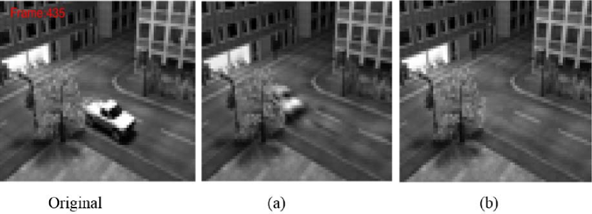
Figure 1: The effect of using weights in sWLR algorithm on the Basic scenario. Frame number 435. Background estimation using sWLR with: (a) $(W_{1})_{ij}\in[5,10]$, (b) $(W_{1})_{ij}\in[500,1000].$ In (a) the estimated background has blurry patches of the foreground object, but as we increase the weights, the foreground object disappears in (b).

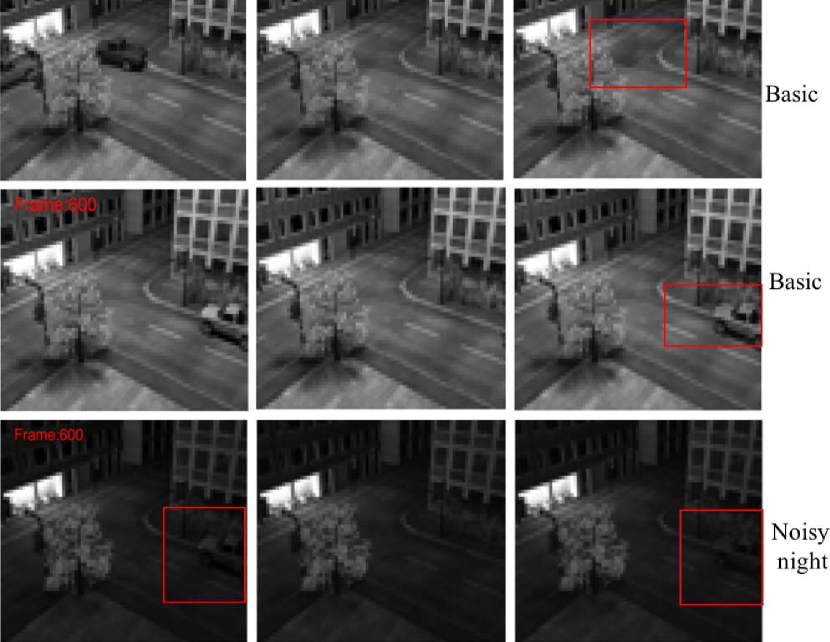
Figure 2: Qualitative analysis of the background estimated by sWLR and APG on the Basic and Noisy night scenario. Frame number 600 has static foreground in both scenarios. APG can not remove the static foreground object from the background. On the other hand, in frame number 210, the low-rank background estimated by APG has still some black patches. In both scenarios sWLR can completely remove the static foreground.

This special choice of the weight is justified as follows: in background subtraction, we only need to put large weights on the columns (frames) that are more likely to be the background and leave the rest of the columns unweighted (and thus with weight $1$). Our new algorithm is not based on matrix factorization to address the rank constraint [3]. Instead, we exploit the dependence of ${X}_{2}$ on ${X}_{1}$ in the optimal solution. We will use Theorem 2 to device an iterative process to solve (5). We assume that ${\rm r}({X}_{1})=k.$ Then any ${X}_{2}$ such that ${\rm r}({X}_{1}\;\;{X}_{2})\leq r$ can be given in the form

$${X}_{2}={X}_{1}C+D,$$

for some arbitrary matrices $C\in\mathbb{R}^{k\times(n-k)}$ and $D\in\mathbb{R}^{m\times(n-k)}$, such that ${\rm r}(D)\leq r-k$. Therefore, (5) becomes an constrained weighted low-rank approximation problem:

$$\min_{\begin{subarray}{c}{X}_{1},C,D\\ {\rm r}(D)\leq r-k\end{subarray}}\left(\|(A_{1}-{X}_{1})\odot W_{1}\|_{F}^{2}+\|A_{2}-{X}_{1}C-D\|_{F}^{2}\right).$$ (8)

Denote $F({X}_{1},C,D)=\|(A_{1}-{X}_{1})\odot W_{1}\|_{F}^{2}+\|A_{2}-{X}_{1}C-D\|_{F}^{2}$ as the objective function. Assume that at the $p$-th step we have $(X_{1})_{p}$. We need to find $(C_{p},D_{p})$ by solving

$$\min_{C,D}F((X_{1})_{p},C,D).$$

Then Theorem 2 suggests  

$$(X_{1})_{p}C_{p}=P_{(X_{1})_{p}}(A_{2})~{}{\rm and}~{}D_{p}=H_{r-k}(P_{(X_{1})_{p}}^{\perp}(A_{2})).$$

So, if $(X_{1})_{p}$ has its QR decomposition:  

$$(X_{1})_{p}=Q_{p}R_{p},$$

then

$$C_{p}=R_{p}^{-1}Q_{p}^{T}A_{2}$$

and  

$$D_{p}=H_{r-k}((I-Q_{p}Q_{p}^{T})A_{2})=U_{p}(\Sigma_{p})_{r-k}V_{p}^{T},$$

with $U_{p}\Sigma_{p}V_{p}^{T}$ being a SVD of $(I-Q_{p}Q_{p}^{T})A_{2}$.

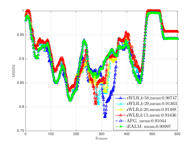
(a) Basic

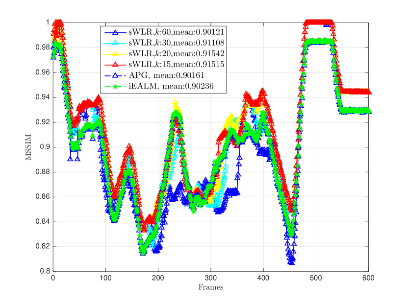
(b) Noisy night

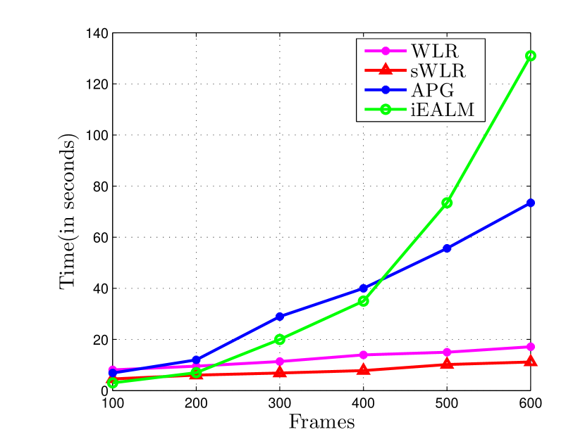
(c)

Figure 3: Mean SSIM of different methods on: (a) Basic and (b) Noisy night scenario. The choice of $k$ for sWLR is critical and empirically determined. However, sWLR has better MSSIM compare to RPCA algorithms corresponding to the frames which has static foreground (frame numbers 551 to 600) or no foreground (frame numbers 6 to 12 and 483 to 528). (c) Number of video frames vs. computation time on the Basic sequence. As the number of video frame increases RPCA algorithms show an exponential increment in computational time. For both WLR and sWLR, $k=15$, $r=k+1$.

We are only left to find $({X}_{1})_{p+1}$ given $(C_{p},D_{p})$ via the following iterative scheme:

$$\displaystyle{({X}_{1})_{p+1}=\arg\min_{{X}_{1}}F({X}_{1},C_{p},D_{p})}.$$ (9)

We will update ${X}_{1}$ row-wise. Let ${X}_{1}(i,:)$ denote the $i$-th row of the matrix ${X}_{1}$. We set $\frac{\partial}{\partial{X}_{1}}F({X}_{1},C_{p},B_{p})=0$ and obtain

$$-(A_{1}-{X}_{1})\odot W_{1}\odot W_{1}-(A_{2}-{X}_{1}C_{p}-D_{p})C_{p}^{T}=0.$$

Solving the above expression for ${X}_{1}$ sequentially along each row produces

$$({X}_{1}(i,:))_{p+1}= (E(i,:))_{p}({\rm diag}(W_{1}^{2}(i,1)$$

$$\;\;W_{1}^{2}(i,2)\cdots W_{1}^{2}(i,k))+C_{p}C_{p}^{T})^{-1},$$

where $E_{p}=A_{1}\odot W_{1}\odot W_{1}+(A_{2}-D_{p})C_{p}^{T}$. Therefore, we have the following algorithm.

1 Input : $A=(A_{1}\;\;A_{2})\in\mathbb{R}^{m\times n}$ (the given matrix); $W=(W_{1}\;\;\mathbf{1})\in\mathbb{R}^{m\times n},$ (the weight); threshold $\epsilon>0$;

2 Initialize : $(X_{1})_{0}$;

3 while not converged do

      4 $({X}_{1})_{p}=Q_{p}R_{p}$, $(I_{m}-Q_{p}Q_{p}^{T})A_{2}=U_{p}\Sigma_{p}V_{p}^{T}$;

      5 $C_{p}=R_{p}^{-1}Q_{p}^{T}A_{2}$;

      6 $D_{p}=U_{p}(\Sigma_{p})_{r-k}V_{p}^{T}$;

      7 $E_{p}=A_{1}\odot W_{1}\odot W_{1}+(A_{2}-D_{p})C_{p}^{T}$;

      8 for $i=1:m$ do

            9 $({X}_{1}(i,:))_{p+1}=(E(i,:))_{p}({\rm diag}(W_{1}^{2}(i,1)\newline \makebox[8.5359pt]{}\;\;W_{1}^{2}(i,2)\cdots W_{1}^{2}(i,k))+C_{p}C_{p}^{T})^{-1}$;

            

       end for

      10$p=p+1$;

      

end while

11Output : $(X_{1})_{p},(X_{1})_{p}C_{p}+D_{p}.$

Algorithm 1 sWLR Algorithm

The update rule for Algorithm sWLR is

$${X}_{p+1}=(({X}_{1})_{p}\;\;({X}_{1})_{p}C_{p}+D_{p}),$$

with ${\rm r}(({X}_{1})_{p})=k$, ${\rm r}(({X}_{1})_{p}C_{p})\leq k$, ${\rm r}(D_{p})\leq r-k$, and so, ${\rm r}({X}_{p+1})\leq r$.

4 Numerical Experiments

In this section we will demonstrate the performance of our algorithm in solving the background estimation problem and compare it with WLR in [3] and the RPCA methods [5, 17, 10].

4.1 Implementation Details

Let $X_{sWLR}=({X}_{1}^{*}\;\;{X}_{1}^{*}C^{*}+D^{*})$ where $({X}_{1}^{*},C^{*}$, $D^{*})$ is a solution to (8). We denote $X_{p}$ as our approximation to $X_{sWLR}$ at $p$th iteration. Recall that $X_{p}=(({X}_{1})_{p}\;\;({X}_{1})_{p}C_{p}+D_{p}).$ We denote $\|X_{p+1}-X_{p}\|_{F}=Error_{p}$ and use $\frac{\|Error_{p}\|_{F}}{\|X_{p}\|_{F}}$ as a measure of the relative error. For a threshold $\epsilon>0$ the stopping criteria of our algorithm at the $(p+1)$th iteration is $\|Error_{p}\|_{F}<\epsilon$ or $\frac{\|Error_{p}\|_{F}}{\|X_{p}\|_{F}}<\epsilon$ or if the maximum iterations attained. The algorithm performs the best when we initialize ${X}_{1}$ as a random matrix and takes 5–10 iterations to converge.

Recall that, the Robust PCA (RPCA) method for background estimation problems uses the fact that the background frames, $X$, have a low-rank structure and the foreground $A-X$ is sparse [5, 17, 10] and solves:

$$\min_{X}\{\|A-X\|_{\ell_{1}}+\lambda\|X\|_{*}\}.\vspace{-0.04in}$$ (10)

For RPCA, we use the inexact augmented Lagrange multiplier (iEALM) method proposed by Lin et. al.  [5], and the accelerated proximal gradient (APG) algorithm proposed by Wright et. al.  [17]. For iEALM and APG we set $\lambda={1}/{\sqrt{{\rm max}\{m,n\}}}$, and for iEALM we choose $\mu=1.5,\rho=1.25$ [5, 10, 17]. A threshold equal to $10^{-7}$ is set for all algorithms.

4.2 Experimental Setup

We perform our experiments on the Stuttgart synthetic video data set [16]. It is a computer generated video sequence, that comprises gradual or sudden change of illumination, a dynamic background containing non-stationary objects and a static foreground, camouflage, and sensor noise or compression artifacts. We perform qualitative and quantitative analysis on two different test scenarios of the sequence: (i) Basic and (ii) Noisy night. Each scenario has 600 frames with identical foreground and background objects. Frame numbers 551 to 600 have static foreground, and frame numbers 6 to 12 and 483 to 528 have no foreground. Additionally, the foreground comes with high quality ground truth mask for each video frame.

4.3 Comparison between RPCA and sWLR

In Figure 1, we demonstrate the effects of using big weights on the frames in the first block $X_{1}$ for sWLR. With proper choice of $r$ and $k$ the large weights in $W_{1}$ produces a better background estimation. In Figure 2, we present qualitative comparison between the background estimated by sWLR and RPCA algorithms. Since APG and iEALM both have same reconstruction we only present APG here. In both scenarios, sWLR provides a substantially better background estimation than APG.

For quantitative comparison between different methods we use the most advanced measure structural similarity index (SSIM) in Figure 3(a) and (b). According to [11], the SSIM index can be viewed as a robust quality measure of a recovered image, compare to the other image that is regarded as of perfect quality. It compares the luminance change, contrast change, and structural change in the recovered image and agree with human visual perception the most compare to any other standard measures. Our background estimation experiments for sWLR are based on a prior knowledge of the background frame indexes. From the ground truth, we know that the entire sequence has 60 foreground frames that has less than 10 pixels. Given 60 pure background frames we choose $k=\Bigl{\lceil}60/i_{1}\Bigr{\rceil}$ by random sampling, where $i_{1}\in\{1,2,3,4\}$. We set $r=k+1$. For Basic and Noisy night $k=15$ and $k=20$ respectively, are the best choice. Since the qualitative and quantitative results for background estimation are same for both WLR and sWLR we only provide their runtime comparison (see Figure 3 (c)). In Figure 3(c), the increment in time for the RPCA algorithms as we increase the dimension of the test matrix by adding more frames can be attributed by computation of a larger rank SVD in each step of their iteration. On the other hand, sWLR performs a fixed rank SVD once the background frames are learned.

5 Conclusion

In this paper we presented a simple and fast numerical algorithm to solve a weighted low rank approximation problem for a special family of weights. To demonstrate its use in the real world problems we performed background estimation from video sequences when a prior knowledge of approximated background fames is available. We did not address the question on how to automatically learn the weight from the data which is treated in [3]. The performance of our weighted low-rank approximation algorithm over the existing RPCA algorithms shows the fact that a weighted Frobenius norm can be made robust to sparse outliers. With additional knowledge of some approximate frames learned from the data, our algorithm can outperform the RPCA algorithms in terms of accuracy and efficiency.

References

- [1] G. H. Golub, A. Hoffman, and G. W. Stewart, “A generalization of the Eckart-Young-Mirsky matrix approximation theorem", Linear Algebra and its Applications, vol. 88-89, pp. 317–327, 1987.
- [2] A. Dutta and X. Li, “On a problem of weighted low rank approximation of matrices", SIAM Journal on Matrix Analysis and Applications, to appear.
-
[3]
A. Dutta and X. Li, “Weighted low rank approximation for background estimation problems", submitted,
2017. - [4] I. T. Jolliffee, “Principal Component Analysis”, Second edition, Springer-Verlag, 2002.
- [5] Z. Lin, M. Chen, and Y. Ma,“The augmented Lagrange multiplier method for exact recovery of corrupted low-rank matrices", arXiv1009.5055, 2010.
- [6] N. Srebro and T. Jaakkola,“Weighted low-rank approximations”, 20th International Conference on Machine Learning, pp. 720–727, 2003.
- [7] T. Okatani and K. Deguchi, “On the Wiberg algorithm for matrix factorization in the presence of missing components," International Journal of Computer Vision, vol. 72, no. 3, pp. 329–337, 2007.
- [8] T. Wiberg, “Computation of principal components when data are missing,” In Proceedings of the Second Symposium of Computational Statistics, pp. 229–336, 1976.
- [9] I. Markovsky, J. C. Willems, B. De Moor, and S. Van Huffel, “Exact and approximate modeling of linear systems: a behavioral approach," SIAM, 2006.
- [10] E. J. Candès, X. Li, Y. Ma, and J. Wright, “Robust principal component analysis?", Journal of the Association for Computing Machinery, vol. 58, no. 3, pp. 11:1–11:37, 2011.
- [11] Z. Wang, A. C. Bovik, H. R. Sheikh, and E. P. Simoncelli, “Image quality assessment: from error visibility to structural similarity," IEEE Transaction on Image Processing, vol. 13, no. 4, pp. 600–612, 2004.
- [12] J. H. Manton, R. Mehony, and Y. Hua, “The geometry of weighted low-rank approximations," IEEE Transactions on Signal Processing, vol. 51, no. 2, pp. 500–514, 2003.
- [13] W. S. Lu, S. C. Pei, and P. H. Wang, “Weighted low-rank approximation of general complex matrices and its application in the design of 2-D digital filters”, IEEE Transactions on Circuits and Systems I: Fundamental Theory and Applications, vol. 44, no. 7, pp.650–655,1997.
- [14] D. Shpak, “A weighted-lesat-squares matrix decomposition with application to the design of 2-D digital filters", In Proceedings of IEEE 33rd Midwest Symposium on Circuits and Systems, pp. 1070–1073, 1990.
- [15] N. Oliver, B. Rosario, and A. Pentland, “A Bayesian Computer vision system for modeling human interactions”, IEEE Transactions on Pattern Analysis and Machine Intelligence, vol. 22, no. 8, pp. 831–843, 2000.
- [16] S. Brutzer, B. Höferlin, and G. Heidemann,“Evaluation of background subtraction techniques for video surveillance”, IEEE Computer Vision and Pattern Recognition, pp. 1937-1944, 2011.
-
[17]
J. Wright, Y. Peng, Y. Ma, A. Ganseh, and S. Rao,
“Robust principal component analysis: exact recovery of corrupted low-rank matrices by convex optimization",Advances in Neural Information Processing Systems, vol. 22, pp. 2080–2088, 2009.