Testing Holographic Conjectures of Complexity with Born-Infeld Black Holes

Abstract

In this paper, we use Born-Infeld black holes to test two recent holographic conjectures of complexity, the “Complexity = Action” (CA) duality and “Complexity = Volume 2.0” (CV) duality. The complexity of a boundary state is identified with the action of the Wheeler-deWitt patch in CA duality, while this complexity is identified with the spacetime volume of the WdW patch in CV duality. In particular, we check whether the Born-Infeld black holes violate the Lloyd bound: $\mathcal{\dot{C}\leq}\frac{2}{\pi\hbar}\left[\left(M-Q\Phi\right)-\left(M-Q\Phi\right)_{\text{gs}}\right]$, where gs stands for the ground state for a given electrostatic potential. We find that the ground states are either some extremal black hole or regular spacetime with nonvanishing charges. Near extremality, the Lloyd bound is violated in both dualities. Near the charged regular spacetime, this bound is satisfied in CV duality but violated in CA duality. When moving away from the ground state on a constant potential curve, the Lloyd bound tend to be saturated from below in CA duality, while $\mathcal{\dot{C}}$ is $\pi/2$ times as large as the Lloyd bound in CV duality.

I Introduction

Through gauge/gravity duality, concepts from quantum information theory have driven major advances in our understanding of quantum field theory and quantum gravity. For example, the holographic entanglement entropy IN-Ryu:2006bv ; IN-Ryu:2006ef has been currently receiving considerable attentions in the ongoing research. Recently inspired by the observation that the size of the Einstein-Rosen bridge (ERB) grows linearly at late times, it was conjectured IN-Susskind:2014rva ; IN-Stanford:2014jda ; IN-Susskind:2014jwa ; IN-Susskind:2014moa that quantum complexity of a boundary state is dual to the volume of the maximal spatial slice crossing the ERB anchored at the boundary state. Roughly speaking, the complexity $\mathcal{C}$ of a state is the minimum number of quantum gates to prepare this state from a reference state IN-Wat:2009 ; IN-Huang:2015 ; IN-Osb:2011 . However, one of unappealing features of this proposal is that there is an ambiguity in choosing a length scale in the bulk geometry, which provides some motivations to introduce the “Complexity = Action” (CA) duality IN-Brown:2015bva ; IN-Brown:2015lvg .

In CA duality, the complexity of a boundary state is identified with the action of the Wheeler-DeWitt (WdW) patch in the bulk:

$$\mathcal{C=}\frac{S_{\text{WdW}}}{\pi\hbar},$$ (1)

where the WdW patch can be defined as the domain of dependence of any Cauchy surface anchored at the boundary state. After the original calculations of $S_{\text{WdW}}$ in IN-Brown:2015lvg , a detailed analysis was carried out in IN-Lehner:2016vdi , of the contributions to the action of some subregion from a null segment and a joint at which a null segment is joined to another segment. It is interesting to note that although the two approaches used in IN-Brown:2015lvg and IN-Lehner:2016vdi are different, the results for $dS_{\text{WdW}}/dt$ at late times of the AdS Schwarzschild and Reissner-Nordstrom (RN) AdS black holes turn out to be the same. A possible explanation was given in IN-Lehner:2016vdi .

Similar to the holographic entanglement entropy, the holographic complexity in CA duality is divergent, which is related to the infinite volume near the boundary of AdS space. The divergent terms were considered in IN-Carmi:2016wjl ; IN-Reynolds:2016rvl ; IN-Kim:2017lrw , which showed that these terms could be written as local integrals of boundary geometry. This implies that the divergence comes from the UV degrees of freedom in the field theory. On the other hand, there are two finite quantities associated with the complexity, which can be calculated without first obtaining these divergent terms. The first one is the “complexity of formation” IN-Chapman:2016hwi , which is the difference of the complexity between a particular black hole and a vacuum AdS spacetime. The second one is the rate of complexity at late times, $\mathcal{\dot{C}}$. If CA duality is correct, $\mathcal{\dot{C}}$ should saturate the Lloyd bound IN-Llo:2000 . The Lloyd bound is the conjectured complexity growth bound, which states that $\mathcal{\dot{C}}$ should be bounded by the energy IN-Brown:2015lvg :

$$\mathcal{\dot{C}\leq}\frac{2E}{\pi\hbar}.$$ (2)

For a black hole, $E$ is its mass $M$, and the Lloyd bound then reads

$$\mathcal{\dot{C}\leq}\frac{2M}{\pi\hbar}.$$ (3)

As noted in IN-Brown:2015lvg , the rate of the complexity of a neutral black hole is faster than that of a charged black hole since the existence of conserved charges could put constraints on the system. That implies that the Lloyd bound can be generalized for a charged black hole with the charge $Q$ and potential at the horizon $\Phi$:

$$\mathcal{\dot{C}\leq}\frac{2}{\pi\hbar}\left[\left(M-Q\Phi\right)-\left(M-Q\Phi\right)_{\text{gs}}\right],$$ (4)

where $\left(M-Q\Phi\right)_{\text{gs}}$ is $M-Q\Phi$ calculated in the ground state. A similar bound can also be given for rotating black holes IN-Brown:2015lvg .

The rate of complexity in CA duality has been considered in several examples. In IN-Brown:2015lvg , it showed that neutral black holes, rotating BTZ black holes, and small RN AdS black holes saturated the corresponding Lloyd bounds, while intermediate and large RN AdS black holes violated the bound $\left(\ref{eq:LBoundQ}\right)$. Later, it was pointed out IN-Cai:2016xho ; IN-Couch:2016exn that even the small RN AdS black holes also violated the bound $\left(\ref{eq:LBoundQ}\right)$. The WdW patch action growth of RN AdS black holes, (charged) rotating BTZ black holes, AdS Kerr black holes, and (charged) Gauss-Bonnet black holes were calculated in IN-Cai:2016xho . The action growth was also discussed in case of massive gravities IN-Pan:2016ecg and higher derivative gravities IN-Alishahiha:2017hwg . A general case was considered in IN-Huang:2016fks , and it was proved that the action growth rate equals the difference of the generalized enthalpy at the outer and inner horizons. While this paper is in preparation, a preprint IN-Cai:2017sjv appeared calculating the action growth of Born-Infeld black holes, charged dilaton black holes, and charged black holes with phantom Maxwell field in AdS space. It also showed there that a Born-Infeld AdS black hole with a single horizon and a charged dilaton AdS black hole satisfied the Lloyd bound $\left(\ref{eq:LBound}\right)$, while for the charged black hole with a phantom Maxwell field, this bound was violated.

Noting that the thermodynamic volume was related to the linear growth of the WdW patch at late times, Couch et. al. proposed “Complexity = Volume 2.0” duality in IN-Couch:2016exn . In “Complexity = Volume 2.0” (CV) duality, the complexity is identified with the spacetime volume of the WdW patch. It was found that the Lloyd bound $\left(\ref{eq:LBoundQ}\right)$ was violated in both CA and CV dualities for RN AdS black holes near extremality. However if the ground state was an empty AdS space, this bound was violated in CA duality but satisfied in CV duality. In what follows, let $\mathcal{C}_{A}/\mathcal{C}_{V}$ denote the complexity calculated in CA/CV duality.

In this paper, we will check whether the generalized Lloyd bound $\left(\ref{eq:LBoundQ}\right)$ is violated for the Born-Infeld AdS black holes in CA and CV dualities. The remainder of our paper is organized as follows. In section II, we discuss some properties of Born-Infeld AdS black holes, which could have a naked singularity, a single horizon, or two horizons depending on their parameters. The phase diagrams for these black holes are obtained. In section III, we consider the Lloyd bound for the Born-Infeld AdS black holes in CA/CV dualities. In section IV, we conclude with a brief discussion of our results. In the appendix, we employ the approach in IN-Lehner:2016vdi to calculate action growth for $\left(d+1\right)$-dimensional Born-Infeld AdS black holes with hyperbolic, planar, and spherical horizons.

II Born-Infeld AdS Black Holes

In this section, we will consider the black hole solutions of Einstein-Born-Infeld action in $\left(d+1\right)$ dimension $\left(d\geq 3\right)$ with a negative cosmological constant $\Lambda=-\frac{d\left(d-1\right)}{L^{2}}$. The action of Einstein gravity and Born-Infeld field reads

$$S=\int_{\mathcal{M}}d^{d+1}x\sqrt{-g}\left(R+\frac{d\left(d-1\right)}{L^{2}}\right)+\int_{\mathcal{M}}d^{d+1}x\sqrt{-g}L\left(F\right),$$ (5)

where we take $16\pi G=1$ for simplicity, $L\left(F\right)$ is given by

$$L\left(F\right)=4\beta^{2}\left(1-\sqrt{1+\frac{F^{\mu\nu}F_{\mu\nu}}{2\beta^{2}}}\right),$$ (6)

and, $\beta$ is the Born-Infeld parameter. When $\beta\rightarrow\infty$, the Lagrangian of Born-Infeld field $L\left(F\right)$ becomes that of standard Maxwell field, $L\left(F\right)=-F^{\mu\nu}F_{\mu\nu}.$ The static black hole solution was obtained in BIABH-Dey:2004yt ; BIABH-Cai:2004eh :

$$ds^{2} =-f\left(r\right)dt^{2}+\frac{dr^{2}}{f\left(r\right)}+r^{2}d\Sigma_{k,d-1}^{2},$$

$$F^{rt} =\frac{\sqrt{\left(d-1\right)\left(d-2\right)}\beta q}{\sqrt{2\beta^{2}r^{2d-2}+\left(d-1\right)\left(d-2\right)q^{2}}},$$ (7)

where

$$f\left(r\right) =k-\frac{m}{r^{d-2}}+\left[\frac{4\beta^{2}}{d\left(d-1\right)}+\frac{1}{L^{2}}\right]r^{2}-\frac{2\sqrt{2}\beta}{d\left(d-1\right)r^{d-3}}\sqrt{2\beta^{2}r^{2d-2}+\left(d-1\right)\left(d-2\right)q^{2}}$$

$$+\frac{2\left(d-1\right)q^{2}}{dr^{2d-4}}\text{ }_{2}F_{1}\left[\frac{d-2}{2d-2},\frac{1}{2},\frac{3d-4}{2d-2},-\frac{\left(d-1\right)\left(d-2\right)q^{2}}{2\beta^{2}r^{2d-2}}\right],$$ (8)

and, $d\Sigma_{k,d-1}^{2}$ is the line element of the $\left(d-1\right)$-dimensional hypersurface with constant scalar curvature $\left(d-1\right)\left(d-2\right)k$ with $k=\left\{-1,0,1\right\}$. Note that the black holes with $k=\left\{-1,0,1\right\}$ have hyperbolic, planar, and spherical horizons. The mass $M$ and charge $Q$ of the Born-Infeld black hole are given by, respectively,

$$M =\left(d-1\right)\Omega_{k,d-1}m,$$

$$Q =\frac{\sqrt{\left(d-1\right)\left(d-2\right)}\Omega_{k,d-1}}{4\pi\sqrt{2}}q,$$ (9)

where $\Omega_{k,d-1}$ denotes the dimensionless volume of $d\Sigma_{k,d-1}^{2}$. For $k=0$ and $-1$, one needs to introduce an infrared regulator to produce a finite value of $\Omega_{k,d-1}$.

For the sake of calculating the action growth and thermodynamic volume of the Born-Infeld black holes, we need to determine the number of their horizons. Depending on the values of the parameters $q$ and $m$, the black holes could possess a naked singularity at $r=0$, one, or two horizons. In fact, we could define a $q$-dependent function

$$m\left(r,q\right)=r^{d-2}f\left(r\right)+m,$$ (10)

which does not depend on the parameter $m$. For a given value of $m$, one could solve $m\left(r,q\right)=m$ for the position of the horizon. The derivative of $m\left(r,q\right)$ with respect to $r$ is

$$\frac{dm\left(r,q\right)}{dr}=\left(d-2\right)r^{d-3}\left[k+\frac{dr^{2}}{\left(d-2\right)L^{2}}-\frac{2q^{2}}{r^{d+1}\left(r^{d-1}+\sqrt{r^{2d-2}+\frac{\left(d-1\right)\left(d-2\right)q^{2}}{2\beta^{2}}}\right)}\right],$$ (11)

which is a strictly increasing function. When $r\rightarrow\infty$, $dm\left(r,q\right)/dr$ goes to $\infty$. In the limit $r\rightarrow 0$, we find that

$$\frac{dm\left(r,q\right)}{dr}|_{r=0} =-\frac{2\sqrt{2}\beta q}{\left(d-1\right)}\sqrt{\left(d-1\right)\left(d-2\right)},\text{ for }d>3\text{,}$$

$$\frac{dm\left(r,q\right)}{dr}|_{r=0} =k-2\beta q\text{, for }d=3,$$ (12)

which shows that $dm\left(r,q\right)/dr|_{r=0}\geq 0$ in the $k=1$, $d=3$, and $\beta q\leq 1/2$ case, and $dm\left(r,q\right)/dr|_{r=0}<0$ in the other cases. When $\frac{dm\left(r,q\right)}{dr}|_{r=0}<0$, the equation $dm\left(r,q\right)/dr=0$ has one and only solution $r_{e}\left(q\right)>0$, such that $dm\left(r,q\right)/dr|_{r=r_{e}\left(q\right)}=0$. Thus, there is an extremal black hole solution with the parameter $m=m\left(r_{e}\left(q\right),q\right)$ and the horizon being at $r=r_{e}\left(q\right)$. At $r=r_{e}\left(q\right)$, we obtain

$$m\left(r_{e}\left(q\right),q\right)=\frac{2}{d}kr_{e}^{d-2}+\frac{2\left(d-1\right)q^{2}}{dr_{e}^{d-2}}\text{ }_{2}F_{1}\left[\frac{d-2}{2d-2},\frac{1}{2},\frac{3d-4}{2d-2},-\frac{\left(d-1\right)\left(d-2\right)q^{2}}{2\beta^{2}r_{e}^{2d-2}}\right].$$ (13)

When $k=0$ and $1$, $m\left(r_{e}\left(q\right),q\right)$ is always positive. However for $k=-1$, $m\left(r_{e}\left(q\right),q\right)$ could be negative for some values of $q$. It is noteworthy that $m\left(r_{e}\left(q\right),q\right)$ exists for $q\geq\frac{1}{2\beta}$ in the $k=1$, $d=3$, and $\beta q\leq 1/2$ case, while $m\left(r_{e}\left(q\right),q\right)\,$ exists for all values of $q$ in other cases. Moreover, one finds that

$$m\left(0,q\right)=A\left(q\right)>0,$$ (14)

where

$$A\left(q\right)\equiv\frac{2\left(d-1\right)q^{2}}{d}\frac{\Gamma\left(\frac{3d-4}{2d-2}\right)\Gamma\left(\frac{1}{2\left(d-1\right)}\right)}{\sqrt{\pi}}\left[\frac{2\beta^{2}}{\left(d-1\right)\left(d-2\right)q^{2}}\right]^{\frac{d-2}{2\left(d-1\right)}}.$$ (15)

Since $dm\left(r,q\right)/dr<0$ for $0<r<r_{e}$, one obtains $m\left(r_{e}\left(q\right),q\right)<m\left(0,q\right)=A\left(q\right)$. In FIG. 1, we plot the function $m\left(r,q\right)$ against $r$ for different values of $q$, where we take $L=1$ and $\beta=10$.

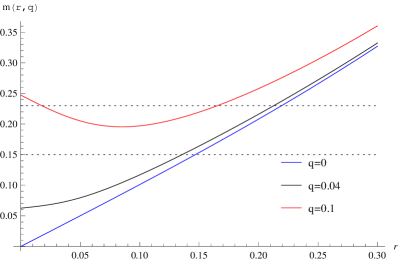
(a)   $k=1$ and $d=3$

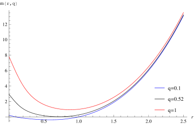
(b)  $k=-1$ and $d=3$

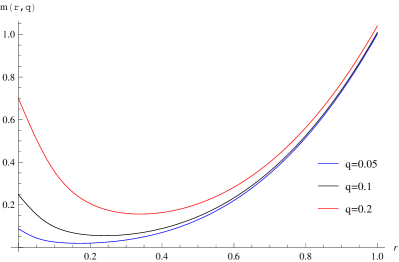
(c)   $k=0$ and $d=3$

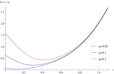
(d)   $k=1$ and $d=4$

Figure 1: Plots of $m\left(r,q\right)$ versus $r$ for different values of $q$, where $L=1$ and $\beta=10$.

With the above results, we can discuss when the Born-Infeld black hole solution $\left(\ref{eq:BIBH}\right)$ possesses a naked singularity, a single horizon, or two horizons:

• Single Horizon: $m\geq A\left(q\right)$. For example, $\left\{q=0.04\text{, }m=0.15\right\}$ in FIG. 1(a)

• Two Horizons: $m\left(r_{e}\left(q\right),q\right)\leq m<A\left(q\right)$. For example, $\left\{q=0.1\text{, }m=0.23\right\}$ in FIG. 1(a)

• Naked Singularity: $m<A\left(q\right)$ when $k=1$, $d=3$, and $\beta q\leq 1/2$; $m<m\left(r_{e}\left(q\right),q\right)$ in the other cases. For example, $\left\{q=0.1\text{, }m=0.15\right\}$ in FIG. 1(a).

The phase diagrams for Born-Infeld AdS black holes are plotted in FIG. 2, for the cases with $\left\{d=3\text{, }k=\pm 1,0\right\}$ and $\left\{d=4\text{, }k=1\right\}$. We also take $L=1$ and $\beta=10$ in FIG. 2. The blue lines in FIG. 2 are extremal lines, which are given by $m=$ $m\left(r_{e}\left(q\right),q\right)$. The boundaries between the black holes with one horizon and these with two horizons are depicted as the black dashed lines, which are given by $m=A\left(q\right)$. The colored lines (red and blue) are the boundaries between black holes and naked singularities. In FIG. 2(a), the red line divides the black holes with a single horizon and the spacetime with a naked singularity, and it meets the blue extremal line at the red dot, whose $q\,$coordinate is $\frac{1}{2\beta}=0.05$.

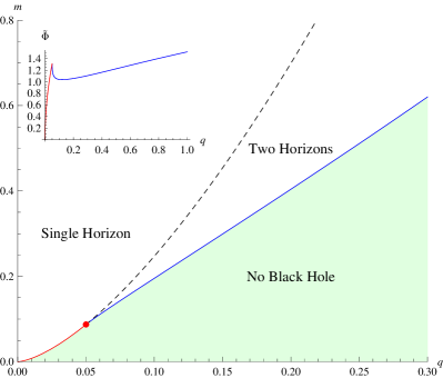
(a)   $k=1$ and $d=3$

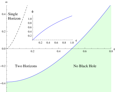
(b)  $k=-1$ and $d=3$

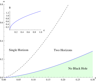
(c)   $k=0$ and $d=3$

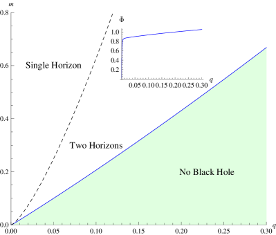
(d)   $k=1$ and $d=4$

Figure 2: The phase diagrams for Born-Infeld AdS black holes where $L=1$ and $\beta=10$. The blue lines are extremal black holes, while the red one is some regular spacetime with nonvanishing charges. Small figures are the plots of the potential along the boundary lines.

To discuss the Lloyd bounds, we need to specify the electrostatic potential of the ground states, which are the colored lines in FIG. 2. The electrostatic potential at the black hole horizon, which is conjugate to the electric charge $Q$, is BIABH-Dey:2004yt ; BIABH-Cai:2004eh

$$\Phi=\sqrt{\frac{d-1}{2\left(d-2\right)}}\frac{16\pi q}{r_{h}^{d-2}}\text{ }_{2}F_{1}\left[\frac{d-2}{2d-2},\frac{1}{2},\frac{3d-4}{2d-2},-\frac{\left(d-1\right)\left(d-2\right)q^{2}}{2\beta^{2}r_{h}^{2d-2}}\right],$$ (16)

where $r_{h}$ is the horizon’s radius. When $\beta\rightarrow\infty$, the Born-Infeld AdS black holes become the RN AdS black holes. When $k=1$ and $d=3$, it was found IN-Brown:2015lvg that the boundary of RN AdS black holes in the phase diagram was the extremal line, and the potential $\Phi$ approached $16\pi$ as $\left(q,m\right)\rightarrow\left(0,0\right)$ along the extremal line. Thus for a RN AdS black hole, the ground state of the geometry with the same electrostatic potential as this black hole is pure AdS spacetime for $\frac{\Phi}{16\pi}\leq 1$, but for $\frac{\Phi}{16\pi}>1$ it is some extremal black hole. Now we compute the asymptotic behavior of $\Phi$ as $\left(q,m\right)\rightarrow\left(0,0\right)$ along the boundaries:

• $k=0$: The boundary is the extremal line, on which $r_{e}\sim q^{\frac{1}{d-1}}$ given by $dm\left(r,q\right)/dr|_{r=r_{e}}=0$. Since $\frac{q^{2}}{r_{e}^{2d-2}}\sim 1$ as $q\rightarrow 0$, we find

  $$\Phi\sim\frac{q}{r_{e}^{d-2}}\sim q^{\frac{1}{d-1}}\rightarrow 0\text{ as }q\rightarrow 0.$$ (17)

• $k=-1\,$: The boundary is the extremal line, on which $r_{e}\sim L$ as $q\rightarrow 0$. One then finds

  $$\Phi\sim\frac{q}{r_{e}^{d-2}}\sim q\rightarrow 0\text{ as }q\rightarrow 0.$$ (18)

  It is interesting to note that

  $$m\rightarrow\frac{2}{d}\left(\frac{d-2}{d}\right)^{\frac{d-2}{2}}L^{d-2}\text{ as }q\rightarrow 0.$$ (19)

• $k=1\,$: If $d>3$, the extremal line could go to $\left(0,0\right)$ as $q\rightarrow 0$. On the extremal line, $dm\left(r,q\right)/dr|_{r=r_{e}}=0$ gives that $r_{e}\sim q^{\frac{1}{d-3}}$ and $\frac{q^{2}}{r_{e}^{2d-2}}\rightarrow\infty$ as $q\rightarrow 0$. Using eqn. $\left(\ref{eq:potential}\right)$, we also find

  $$\Phi\sim q^{\frac{1}{d-1}}\rightarrow 0.$$ (20)

  If $d=3$, the boundary line around $\left(0,0\right)$ is the red line in FIG. 2(a), on which $r_{+}=0$. Again, we have

  $$\Phi\propto q^{\frac{1}{d-1}}\rightarrow 0.$$ (21)

Unlike the $k=1$ and $d=3$ RN AdS black holes, the potential $\Phi\rightarrow 0$ as $\left(q,m\right)\rightarrow\left(0,0\right)$ along the boundary lines for the Born-Infeld AdS black holes. Thus for a Born-Infeld AdS black hole with $\Phi>0$, the ground state of the geometry with the same $\Phi$ is either some extremal black hole (blue lines) or some regular spacetime with nonvanishing charges (red lines). In the cases with $\left\{d=3\text{, }k=\pm 1,0\right\}$ and $\left\{d=4\text{, }k=1\right\}$, the potential along the boundary lines are plotted in FIG. 2, where $\tilde{\Phi}=\frac{\Phi}{16\pi}$, $L=1$, and $\beta=10$.

III Holographic Conjectures of Complexity

In this section, we will discuss CA/CV dualities for the Born-Infeld AdS black holes. In our appendix, the action growth of the Born-Infeld AdS black holes within the WdW patch at late-time approximation is calculated by following the approach in IN-Lehner:2016vdi . The action growth in the case with $k=1$ and $d=3$ was first calculated in IN-Cai:2016xho . The growth rate of the action $dS/dt$ depends on the number of the horizons. In fact, we find that

$$\frac{dS}{dt} =2M-Q\Phi_{+}-\left(d-2\right)A\left(q\right)\Omega_{k,d-1}\text{ in one horizon case,}$$

$$\frac{dS}{dt} =Q\Phi_{-}-Q\Phi_{+}\text{ in two horizons case,}$$ (22)

where $\Phi$ is the potential at the horion given by eqn. $\left(\ref{eq:potential}\right)$, $\Phi_{\pm}$ are $\Phi$ calculated at $r=r_{\pm}$, and $r_{\pm}$ is the radius of the $\genfrac{.}{.}{0.0pt}{}{\text{outer}}{\text{inner}}$ horizon. Furthermore, CA duality indicates that, in the late time regime,

$$\mathcal{\dot{C}}_{A}=\frac{1}{\pi\hbar}\frac{dS}{dt}\text{.}$$ (23)

On the other hand, CV duality gives IN-Couch:2016exn that, in the late time regime,

$$\mathcal{\dot{C}}_{V}=\frac{PV}{\hbar}\text{,}$$ (24)

where $P=d\left(d-1\right)/L^{2}$ is the pressure, and $V$ is the volume of the WdW patch. For Born-Infeld AdS black holes, the rate of the complexity at late times is then given by

$$\mathcal{\dot{C}}_{V} =\frac{\left(d-1\right)\Omega_{k,d-1}r_{+}^{d}}{L^{2}\hbar}\text{ in one horizon case,}$$

$$\mathcal{\dot{C}}_{V} =\frac{\left(d-1\right)\Omega_{k,d-1}\left(r_{+}^{d}-r_{-}^{d}\right)}{L^{2}\hbar}\text{ in two horizons case.}$$ (25)

The Lloyd bound for a charged black hole is

$$\mathcal{\dot{C}\leq}\frac{2}{\pi\hbar}\left[\left(M-Q\Phi\right)-\left(M-Q\Phi\right)_{\text{gs}}\right],$$ (26)

where $\left(M-Q\Phi\right)_{\text{gs}}$ is $M-Q\Phi$ calculated in the ground state. The ground state is on the boundary between black hole region and no black hole region (colored lines in FIG. 2). If the system is treated as a grand canonical ensemble, the ground state has the same potential $\Phi$ as the black hole under consideration. Now we will calculate the rate of the complexity in the CA and CV dualities and check whether the Lloyd bound $\left(\ref{eq:Lbound}\right)$ is violated.

III.1 Around Extremal Line

We first consider a general static charged black hole with the line element

$$ds^{2}=-f\left(r\right)dt^{2}+\frac{dr^{2}}{f\left(r\right)}+r^{2}d\Sigma_{k,d-1}^{2},$$ (27)

where the radii of the outer and inner horizon are $r_{+}$ and $r_{-}$, respectively. The first law of black hole thermodynamics reads

$$dM=TdS+\Phi dQ\text{.}$$ (28)

Since the entropy $S$ is the function of $r_{+}$, one finds

$$\frac{\partial M\left(r_{+},Q\right)}{\partial Q} =\Phi,$$

$$\frac{\partial M\left(r_{+},Q\right)}{\partial r_{+}} =T\frac{dS}{dr_{+}}.$$ (29)

At extremality where $T=0$, we have

$$\frac{\partial M\left(r_{+},Q_{e}\right)}{\partial r_{+}}|_{r_{+}=r_{e}}=0\text{,}$$ (30)

where $r_{e}$ and $Q_{e}$ are the radius and charge, respectively, of the black hole at extremality. For a fixed value of $\Phi$, $r_{+}$ can be determined by $Q\,$: $r_{+}=r_{+}\left(Q\right)$. Thus on the constant $\Phi$ curve near extremality, we find

$$M\left(r_{+}\left(Q_{e}+\delta Q\right),Q_{e}+\delta Q\right)-\left(Q_{e}+\delta Q\right)\Phi-\left[M\left(r_{+}\left(Q_{e}\right),Q_{e}\right)-Q_{e}\Phi\right]$$

$$=\left[\left(\frac{\partial M\left(r_{+},Q\right)}{\partial r_{+}}\frac{dr_{+}\left(Q\right)}{dQ}\right)|_{Q=Q_{e}}\delta Q+\frac{\partial M\left(r_{+},Q\right)}{\partial Q}|_{Q=Q_{e}}\delta Q-\Phi\delta Q\right]+\mathcal{O}\left(\delta Q^{2}\right)\sim\mathcal{O}\left(\delta Q^{2}\right).$$ (31)

The Lloyd bound then becomes

$$\frac{2}{\pi\hbar}\left[\left(M-Q\Phi\right)-\left(M-Q\Phi\right)_{\text{gs}}\right]\sim\mathcal{O}\left(\delta Q^{2}\right)\text{.}$$ (32)

Expanding $r_{\pm}$ near extremality, we find that

$$r_{\pm}\approx r_{e}+c_{1}^{\pm}\delta Q,$$ (33)

where

$$c_{1}^{+} =-\frac{\partial_{Q}\Phi\left(r_{e},Q_{e}\right)}{\partial_{r_{+}}\Phi\left(r_{e},Q_{e}\right)},$$

$$c_{1}^{-} =\frac{\partial_{Q}\Phi\left(r_{e},Q_{e}\right)}{\partial_{r_{+}}\Phi\left(r_{e},Q_{e}\right)}-\frac{2\partial_{r}\Phi\left(r_{e},Q_{e}\right)}{\partial_{r_{+}}^{2}M\left(r_{e},Q_{e}\right)}.$$ (34)

From these we can expand $\mathcal{\dot{C}}$ near extremality as

$$\mathcal{\dot{C}}_{A} \sim\frac{Q_{e}\partial_{r_{+}}\Phi\left(r_{e},Q_{e}\right)}{\pi\hbar}\left(c_{1}^{+}-c_{1}^{-}\right)\delta Q,$$

$$\mathcal{\dot{C}}_{V} \sim\frac{d\left(d-1\right)\Omega_{k,d-1}r_{e}^{d-1}}{L^{2}\hbar}\left(c_{1}^{+}-c_{1}^{-}\right)\delta Q.$$ (35)

If $c_{1}^{+}\neq c_{1}^{-}$, the Lloyd bounds are violated near extremality under the two proposals. For the Born-Infeld AdS black holes with $d=3$, we find that

$$c_{1}^{+}-c_{1}^{-}=\frac{k-\tilde{\Phi}^{2}}{\tilde{\Phi}^{2}\left(k-2\tilde{\Phi}^{2}\right)}-\frac{3\left(k^{2}-8k\tilde{\Phi}^{2}+6\tilde{\Phi}^{4}\right)}{10\beta^{2}L^{2}\left(k-2\tilde{\Phi}^{2}\right)^{2}\left(k-\tilde{\Phi}^{2}\right)}+\mathcal{O}\left(\beta^{-4}\right),$$ (36)

where $\tilde{\Phi}=\frac{\Phi}{16\pi}$.

III.2 Around Regular Charged Spacetime

As shown in FIG. 2(a), there is a red boundary, which is $m=A\left(q\right)$ for $q\leq\frac{1}{2\beta}$, in the case with $d=3$ and $k=1$. Above this boundary, one has a black hole with a single horizon, whose radius goes to zero as approaching the boundary. When $r\ll 1$, we find

$$f\left(r\right)=\left(1-2q\beta\right)-\frac{m-A\left(q\right)}{r}+\mathcal{O}\left(r^{2}\right)\text{,}$$ (37)

which means that the metric is regular at $r=0$ for $m=A\left(q\right)$. Therefore, one has some regular spacetime with nonvanishing charges on the red boundary. The potential $\Phi\left(=16\pi\tilde{\Phi}\right)$ of the ground states on the boundary can be obtained from finding the limit of eqn. $\left(\ref{eq:potential}\right)$ as $r_{+}\rightarrow 0$:

$$\tilde{\Phi}=\tilde{\Phi}_{c}\sqrt{2q\beta}\leq\tilde{\Phi}_{c},$$ (38)

where

$$\tilde{\Phi}_{c}=\frac{1}{\sqrt{2\pi}}\Gamma\left(\frac{5}{4}\right)\Gamma\left(\frac{1}{4}\right)\text{.}$$ (39)

A little bit above the boundary, the radius of a black hole with the potential $\Phi$ is given by

$$r_{+}\approx\frac{\tilde{\Phi}_{c}^{2}}{\tilde{\Phi}^{2}+\tilde{\Phi}_{c}^{2}}\delta m,$$ (40)

where $\delta m=m-m_{0}$, and $m_{0}$ is the $m$ parameter of the ground state with the same potential $\Phi$. Since $r_{+}\ll 1$ implied by eqn. $\left(\ref{eq:rdeltam}\right)$, eqn. $\left(\ref{eq:fnRL}\right)$ gives that the temperature of the black hole is

$$T\propto m-A\left(q\right)\text{,}$$ (41)

which goes to zero as approaching the ground state. For this black hole, we find that the Lloyd bound is

$$\frac{2}{\pi\hbar}\left[\left(M-Q\Phi\right)-\left(M-Q\Phi\right)_{\text{gs}}\right]\approx\frac{16}{\hbar}\left(1-\frac{2\tilde{\Phi}^{2}}{\tilde{\Phi}^{2}+\tilde{\Phi}_{c}^{2}}\right)\delta m.$$ (42)

On the other hand, we can expand $\mathcal{\dot{C}}$ as

$$\mathcal{\dot{C}}_{A} \approx\frac{16}{\hbar}\left(1-\frac{3}{2}\frac{\tilde{\Phi}^{2}}{\tilde{\Phi}^{2}+\tilde{\Phi}_{c}^{2}}\right)\delta m,$$

$$\mathcal{\dot{C}}_{V} \sim\mathcal{O}\left(r_{+}^{3}\right)\sim\mathcal{O}\left(\delta m^{3}\right).$$ (43)

It appears that the bound is satisfied in CV duality although far from saturated near the boundary. However, the bound is violated in CA duality.

III.3 Large $q$ on Constant $\Phi$ Curve

Consider Born-Infeld AdS black holes with fixed potential $\Phi$. When $q\rightarrow\infty$ along the constant $\Phi$ curve, one could have there possibilities for $\frac{q^{2}}{r_{+}^{2d-2}}$: $\frac{q^{2}}{r_{+}^{2d-2}}\rightarrow 0$, $\frac{q^{2}}{r_{+}^{2d-2}}\rightarrow C$ where $0<C<\infty$, and $\frac{q^{2}}{r_{+}^{2d-2}}\rightarrow\infty$. If $\frac{q^{2}}{r_{+}^{2d-2}}\rightarrow\infty$, eqn. $\left(\ref{eq:potential}\right)$ gives that $\Phi$ $\sim q^{\frac{1}{d-1}}$ which can not be a constant. Similarly for $\frac{q^{2}}{r_{+}^{2d-2}}\rightarrow C$, one has that $\Phi\sim r_{+}\sim q^{\frac{1}{d-1}}$. Therefore, we could only have that

$$\frac{q^{2}}{r_{+}^{2d-2}}\rightarrow 0\text{ as }q\rightarrow\infty\text{ along the constant }\Phi\text{ curve.}$$ (44)

Expanding eqn. $\left(\ref{eq:potential}\right)$ in terms of $\frac{q}{r_{+}^{d-1}}$ and solving it for $q$, one has that

$$q\sim\sqrt{\frac{2\left(d-2\right)}{d-1}}\tilde{\Phi}r_{+}^{d-2}\left(1+\frac{\left(d-2\right)^{3}}{2\left(3d-4\right)}\frac{\tilde{\Phi}^{2}}{\beta^{2}r_{+}^{2}}\right).$$ (45)

Since eqn. $\left(\ref{eq:constant phi}\right)$ implies that $r_{+}\gg 1$ when $q\gg 1$, the parameter $m$ is

$$m=\frac{r_{+}^{d}}{L^{2}}\left[1+\mathcal{O}\left(r_{+}^{-2}\right)\right].$$ (46)

The Lloyd bound for $q\gg 1$ $\left(r_{+}\gg 1\right)$ is then given by

$$\frac{2}{\pi\hbar}\left[\left(M-Q\Phi\right)-\left(M-Q\Phi\right)_{\text{gs}}\right]=\frac{2\left(d-1\right)\Omega_{k,d-1}}{\pi\hbar}\frac{r_{+}^{d}}{L^{2}}\left[1+\mathcal{O}\left(r_{+}^{-2}\right)\right].$$ (47)

From eqns. $\left(\ref{eq:constantq}\right)$ and $\left(\ref{eq:constantm}\right)$, it follows that

$$m\sim q^{\frac{d}{d-2}}\text{ for }q\gg 1\text{.}$$ (48)

Since $A\left(q\right)\sim q^{\frac{d}{d-1}}$, the Born-Infeld AdS black holes with fixed potential $\Phi$ always lie above the $m=A\left(q\right)$ line for large enough $q$, which means that these black holes always possess a single horizon for $q\gg 1$ with fixed $\Phi$. Therefore, eqns. $\left(\ref{eq:CA}\right)$ and $\left(\ref{eq:CV}\right)$ give that

$$\mathcal{\dot{C}}_{A} =\frac{2\left(d-1\right)\Omega_{k,d-1}}{\pi\hbar}\frac{r_{+}^{d}}{L^{2}}\left[1-\frac{C_{d}L^{2}\tilde{\Phi}^{\frac{d}{d-1}}\beta^{\frac{d-2}{d-1}}}{2\left(d-1\right)\Omega_{k,d-1}}r_{+}^{\frac{-d}{d-1}}+\mathcal{O}\left(r_{+}^{-2}\right)\right],$$

$$\mathcal{\dot{C}}_{V} =\frac{\left(d-1\right)\Omega_{k,d-1}r_{+}^{d}}{L^{2}\hbar},$$ (49)

where

$$C_{d}=\frac{2\left(d-1\right)}{d}\frac{\Gamma\left(\frac{3d-4}{2d-2}\right)\Gamma\left(\frac{1}{2\left(d-1\right)}\right)}{\sqrt{\pi}}\left(\frac{2}{d-1}\right)^{\frac{d-2}{d-1}}\left[\frac{2\left(d-2\right)}{d-1}\right]^{\frac{1}{d-1}}.$$ (50)

We see immediately that the Lloyd bound is satisfied in CA duality for sufficiently large $q$ and tends to be saturated as $q\rightarrow\infty$. However in CV duality, $\mathcal{\dot{C}}$ is $\pi/2$ times as large as the Lloyd bound for $q\gg 1$.

III.4 Numerical Results

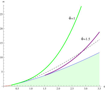
Figure 3: Curves of constant potential $\tilde{\Phi}=1$ and $1.5\,$ in the case with $d=3$, $k=1$, $L=1$ and $\beta=1$.

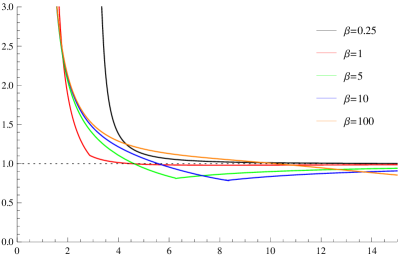
(a)   Plot of $R_{A}$ versus $q$ in CA-duality along the $\tilde{\Phi}=1.5$ curve starting from the extremal boundary.

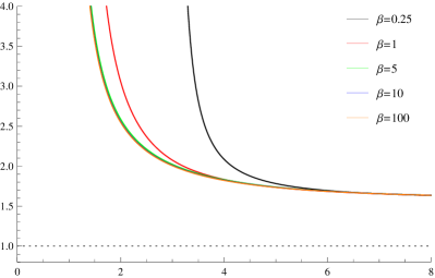
(b)  Plot of $R_{V}$ versus $q$ in CV-duality along the $\tilde{\Phi}=1.5$ curve starting from the extremal boundary.

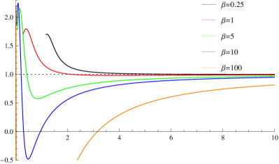
(c)  Plot of $R_{A}$ versus $q$ in CA-duality along the $\tilde{\Phi}=1$ curve starting from the red boundary.

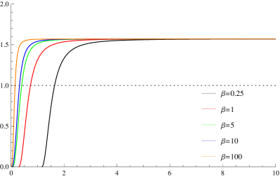
(d)   Plot of $R_{V}$ versus $q$ in CV-duality along the $\tilde{\Phi}=1$ curve starting from the red boundary.

Figure 4: The rate of the complexity in CA-duality and CV-duality divided by the Lloyd bound, $R_{A}$ and $R_{V}$ respectively, along the $\tilde{\Phi}=1$ and $\tilde{\Phi}=1.5$ curves.

Here we consider two curves of constant potential, $\tilde{\Phi}=1$ and $\tilde{\Phi}=1.5$, in the case with $d=3$ and $k=1$. These two constant potential curves are plotted in FIG. 3 for $\beta=1$. Note that the $\tilde{\Phi}=1$ curve (green) starts from some regular spacetime, while the $\tilde{\Phi}=1.5$ curve (purple) starts from some extremal black hole. Both curves enter the “Single Horizon” region for large enough $q$, which is in agreement with the argument below eqn. $\left(\ref{eq:mqL}\right)$.

To check whether the Lloyd bound is violated on the curves, we define

$$R_{A} =\frac{\mathcal{\dot{C}}_{A}}{\frac{2}{\pi\hbar}\left[\left(M-Q\Phi\right)-\left(M-Q\Phi\right)_{\text{gs}}\right]},$$

$$R_{V} =\frac{\mathcal{\dot{C}}_{V}}{\frac{2}{\pi\hbar}\left[\left(M-Q\Phi\right)-\left(M-Q\Phi\right)_{\text{gs}}\right]}.$$ (51)

In FIG. 4, we plot $R_{A}$ and $R_{V}$ along the $\tilde{\Phi}=1$ and $\tilde{\Phi}=1.5$ curves for $\beta=0.25$ (black), $\beta=1$ (red), $\beta=5$ (green), $\beta=10$ (blue), and $\beta=100$ (orange). As shown in FIG. 4, the $R_{A}$ curves approach $R_{A}=1$ asymptotically from below for large $q$, while the $R_{V}$ curves approach $R_{A}=\pi/2$ asymptotically, which agrees with eqns. $\left(\ref{eq:BLQ}\right)$ and $\left(\ref{eq:CLQ}\right)$. Near extremality, $R_{A}$ and $R_{V}$ on the $\tilde{\Phi}=1.5$ curve go to infinity as predicted by eqns. $\left(\ref{eq:bex}\right)$ and $\left(\ref{eq:cex}\right)$. When approaching the red boundary along the $\tilde{\Phi}=1$ curve, $R_{A}$ and $R_{V}$ go above $R_{A}=1$ and to zero, respectively, which also agrees with eqns. $\left(\ref{eq:bRL}\right)$ and $\left(\ref{eq:cRL}\right)$.

Along the $\tilde{\Phi}=1.5$ curve, FIG. 4(a) shows that the Lloyd bound is satisfied in CA duality for large enough $q$, while FIG. 4(b) shows that the Lloyd bound is violated in CV duality. Note that the kinks in the $R_{A}$ curves in FIG. 4(a) are where the $\tilde{\Phi}=1.5$ curve enter the “Single Horizon” region from the ”Two Horizons” region. Along the $\tilde{\Phi}=1$ curve, FIG. 4(d) shows that the Lloyd bound is only satisfied in CV duality for small $q$. It is interesting to see that the $R_{A}$ curves in FIG. 4(c) start to oscillate for small $q$ when $\beta$ is large enough ($\beta=5$, $10$, and $100$). Even for $\beta=10$ and $100$, there is a range of $q$ over which $\mathcal{\dot{C}}_{A}<0$.

In summary, the Lloyd bound is violated in CA duality as we approach the ground states, but this bound tend to be saturated as we go away from the ground states with fixed potential. As noted in IN-Brown:2015lvg , the violations near the ground states have something to do with hair. In CV duality, the Lloyd bound is violated everywhere along the constant potential curves, except near the ground states on the red line.

IV Discussion and Conclusion

In this paper, we first obtained the phase diagram of Born-Infeld AdS black holes and then checked whether the Lloyd bound was violated in CA and CV dualities. In section II, we showed that the Born-Infeld black hole solution could possess a naked singularity, a single horizon, or two horizons, depending on the values of its parameters $q$ and $m$. Except the $k=$ $1$ and $d=3$ case, the boundaries between “Black Hole” region and “No Black Hole” region were extremal lines (blue lines in FIG. 2). However in the $k=$ $1$ and $d=3$ case, there was an additional boundary (red line in FIG. 2(a)), on which were some regular spacetime with nonvanishing charges. It is noteworthy that unlike a RN AdS black hole, the ground state of a Born-Infeld AdS black hole with potential $\Phi>0$ could not be the empty AdS spacetime.

In section III, we calculated the Lloyd bound and the rate of the complexity at late times in CA and CV dualities near the boundaries and for large $q$ on the constant $\Phi$ curves. The results of whether the Lloyd bound was violated are summarized in TABLE 1. We also found that for a general static charged AdS black hole with the charge $Q$ near extremality, the Lloyd bound in eqn. $\left(\ref{eq:Lbound}\right)$ was always $\mathcal{O}\left(\delta Q^{2}\right)$, where $\delta Q\equiv Q-Q_{e}$, and $Q_{e}$ was the charge of the extremal black hole with the same potential. If the difference between the outer and inner horizon radii is $\mathcal{O}\left(\delta Q\right)$, which is the case for RN AdS and Born-Infeld AdS black holes, then the Lloyd bound is usually violated near extremality.

Near Extremal Line Near Red Line Large $q$ on Constant $\Phi$ Curve CA duality Violated Violated Tend to be Saturated CV duality Violated Satisfied Violated   

Table 1: Check of whether Lloyd bound is violated or satisfied.

In the $d=3$ and $k=1$ case, we plotted the rate of the complexity in CA and CV dualities divided by the Lloyd bound along the $\tilde{\Phi}=1$ and $\tilde{\Phi}=1.5$ curves in FIG. 4. It appears that the Lloyd bound in CA duality was violated near the ground states but tended to be saturated as moving away from the ground states along the constant $\Phi$ curves. On the other hand, the Lloyd bound in CV duality was violated along the constant $\Phi$ curves, except near the ground states on the red line. Since the hair may play a role in the violations near the ground states, it seems from these observations that CA duality is slightly favored.

Finally, we want to briefly discuss the differences between our results and these of RN AdS black holes. The ground state of a RN AdS black hole is either the empty AdS space or some extremal black hole. However, the ground state of a Born-Infeld AdS black hole is either some charged regular spacetime or extremal black hole, but could not be the empty AdS space as long as the potential is not zero. As shown by eqn. $\left(5.15\right)$ in IN-Couch:2016exn and FIG. $6$ in IN-Brown:2015lvg , if the ground state was the empty AdS space, $\mathcal{\dot{C}}_{A}$ for a RN AdS black hole with $d=3$ and $k=1$ always violated the Lloyd bound $\left(\ref{eq:LBoundQ}\right)$ along a constant potential curve, even when $q\rightarrow\infty$. However for a Born-Infeld AdS black hole, our results show that the Lloyd bound in CA duality is satisfied for large enough $q$ along a constant potential curve. When $q$ is very large with fixed potential, we have obtained $\frac{q}{r_{+}^{d-1}}\ll 1$, and the metric in eqns. $\left(\ref{eq:BIBH}\right)$ is almost the same as that of a RN AdS black hole outside the outer horizon. In this case, physics over the region outside the outer horizon of the Born-Infeld AdS black hole does not differ much from that of the RN AdS black hole. Different behavior of $\mathcal{\dot{C}}_{A}$ for RN AdS and Born-Infeld AdS black holes with large $q$ on the constant potential curves means that the complexity encodes physics behind black hole horizons.

Appendix A Rate of Action of Born-Infeld AdS Black Holes

In this appendix, we use the methods in IN-Lehner:2016vdi to calculate the change of action, $\delta S=S\left(t_{0}+\delta t\right)-S\left(t_{0}\right)$, of the Wheeler-DeWitt patch at late times. The Penrose diagrams for two-sided eternal Born-Infeld AdS black holes are illustrated in FIG. 5 , along with the Wheeler-DeWitt patches at $t=t_{0}$ and $t_{0}+\delta t$. Here we fix the time on the right boundary and only vary it on the left boundary. There is a divergence appearing when calculating the action near the boundary $r=\infty$. So a surface of constant $r=r_{\max}$ is defined to regulate the action. In IN-Cai:2017sjv , the action was regulated by defining the boundaries of the WdW patch originate slightly inside the AdS boundary. It turns out that these two choices for the regulator yield the same results. We also introduce a spacelike surface $r=\varepsilon$ near the future singularities and let $\varepsilon\rightarrow 0$ at the end of calculations. Note that we have an affine parametrization for each null surface, and these make no contribution to the action. To calculate $\delta S$, we introduce the null coordinates $u$ and $v$ in the metric $\left(\ref{eq:BIBH}\right)$:

$$u =t-r^{\ast}$$

$$v =t+r^{\ast},$$ (52)

where

$$r^{\ast}=\int f^{-1}\left(r\right)dr.$$ (53)

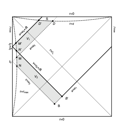
(a)   Single Horizon Case

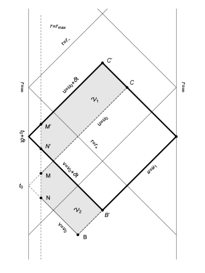
(b)  Two Horizons Case

Figure 5: Wheeler-deWitt patches of Born-Infeld AdS black holes at $t_{L}=t_{0}$ and $t_{L}=t_{0}+\delta t$. The lines $r=r_{\max}$ and $r=\varepsilon$ are cut-off surfaces.

A.1 Single Horizon Case

We calculate $\delta S$ for a Born-Infeld AdS black hole with a single horizon, whose Penrose diagram is illustrated in FIG. 5(a). Due to time translation, the joint contributions from $\mathcal{D}$ and $\mathcal{D}^{\prime}$ are identical, and they therefore make no contribution to $\delta S$. Similarly, the joint and surface contributions from $\mathcal{MN}$ cancel against these from $\mathcal{M}^{\prime}\mathcal{N}^{\prime}$ on $r=r_{\max}$ in calculating $\delta S$. Therefore, we have

$$\delta S=S_{\mathcal{V}_{1}}-S_{\mathcal{V}_{2}}+2\int_{\mathcal{S}}d^{d}x\sqrt{\left|h\right|}K+2\int_{\mathcal{B}^{\prime}}d^{d-1}x\sqrt{\sigma}a-2\int_{\mathcal{B}}d^{d-1}x\sqrt{\sigma}a,$$ (54)

where we follow the conventions in IN-Carmi:2016wjl .

Using the Born-Infeld AdS black hole solution $\left(\ref{eq:BIBH}\right)$, we find that the volume contribution is

$$S_{\mathcal{V}}=\Omega_{k,d-1}\int_{\mathcal{V}}d\omega F\left(r\right),$$ (55)

where $\omega=\left\{u,v\right\}$, and

$$F\left(r\right)=2r^{d-2}\left(k-\frac{m}{r^{d-2}}-f\left(r\right)\right)\text{.}$$ (56)

The region $\mathcal{V}_{1}$ is bounded by the null surfaces $u=u_{0}$, $u=u_{0}+$ $\delta t$, $v=v_{0}+$ $\delta t$, the spacelike surface $r=\varepsilon$, and the timelike surface $r=r_{\max}$. Using eqn. $\left(\ref{eq:SV}\right)$, we have that

$$S_{\mathcal{V}_{1}}=\Omega_{k,d-1}\int_{u_{0}}^{u_{0}+\delta t}duF\left(r\right)|_{\varepsilon}^{\min\left\{r_{\max},\rho\left(u\right)\right\}}dr,$$ (57)

where $r^{\ast}\left(\rho\left(u\right)\right)=\left(v_{0}+\delta t-u\right)/2$. Since $\lim_{r\rightarrow 0}F\left(r\right)=-2A\left(q\right)$, we find that

$$S_{\mathcal{V}_{1}}=\Omega_{k,d-1}\int_{u_{0}}^{u_{0}+\delta t}du\left[F\left(r\right)|_{r=\min\left\{r_{\max},\rho\left(u\right)\right\}}+2A\left(q\right)\right],$$ (58)

where $A\left(q\right)$ is given by eqn. $\left(\ref{eq:Aq}\right)$. Similarly for $\mathcal{V}_{2}$, one has that

$$S_{\mathcal{V}2}=\Omega_{k,d-1}\int_{v_{0}}^{v_{0}+\delta t}dvF\left(r\right)|_{\rho_{1}\left(v\right)}^{\min\left\{r_{\max},\rho_{0}\left(v\right)\right\}},$$ (59)

where $r^{\ast}\left(\rho_{0/1}\left(v\right)\right)=\left(v-u_{0/1}\right)/2$. Performing the change of variables $u=u_{0}+v_{0}+\delta t-v$, we have that

$$\int_{v_{0}}^{v_{0}+\delta t}dvF\left(r\right)|_{r=\min\left\{r_{\max},\rho_{0}\left(v\right)\right\}}=\int_{u_{0}}^{u_{0}+\delta t}duF\left(r\right)|_{r=\min\left\{r_{\max},\rho\left(u\right)\right\}},$$ (60)

and hence

$$S_{\mathcal{V}_{1}}-S_{\mathcal{V}_{2}}=\Omega_{k,d-1}\left[\int_{v_{0}}^{v_{0}+\delta t}dvF\left(r\right)|_{r=\rho_{1}\left(v\right)}+2A\left(q\right)\int_{u_{0}}^{u_{0}+\delta t}du\right].$$ (61)

At late times, one has that $\rho_{1}\left(v\right)\approx r_{+}$, and

$$S_{\mathcal{V}_{1}}-S_{\mathcal{V}_{2}}=\Omega_{k,d-1}\left[F\left(r_{h}\right)+2A\left(q\right)\right]\delta t\text{.}$$ (62)

There is a timelike hypersurface at $r=\varepsilon$, with outward-directed normal vectors from the region of interest. The normal vector is

$$n_{\mu}dx^{\mu}=\frac{-1}{\sqrt{-f\left(r\right)}}dr\text{.}$$ (63)

The trace of extrinsic curvature is

$$K=\frac{1}{r^{d-1}}\partial_{r}\left(r^{d-1}\sqrt{-f\left(r\right)}\right).$$ (64)

Therefore, the surface contributions from $r=\varepsilon$ is

$$2\int_{\mathcal{S}}d^{d}x\sqrt{\left|h\right|}K=2\left(m-A\left(q\right)\right)\Omega_{k,d-1}\frac{\delta t}{r^{d/2-1}}\partial_{r}\left(r^{d/2}\right)|_{r=\varepsilon}=\left[m-A\left(q\right)\right]d\Omega_{k,d-1}\delta t,$$ (65)

where we use $\sqrt{\left|h\right|}=\sqrt{-f\left(r\right)}r^{d-1}d\Omega_{k,d-1}$.

Following IN-Carmi:2016wjl , the integrand $a$ in the joint terms of eqn. $\left(\ref{eq:deltaS}\right)$ is

$$a =\epsilon\ln\left|\mathbf{k}_{1}\cdot\mathbf{k}_{2}/2\right|,$$

$$\epsilon =-\text{sign}\left(\mathbf{k}_{1}\cdot\mathbf{k}_{2}\right)\text{sign}\left(\mathbf{\hat{k}}\cdot\mathbf{k}_{2}\right),$$ (66)

where for $\mathcal{B}$ and $\mathcal{B}^{\prime}$,

$$\left(\mathbf{k}_{1}\right)_{\mu} =-c_{1}\partial_{\mu}\left(t+r^{\ast}\right),$$

$$\left(\mathbf{k}_{2}\right)_{\mu} =c_{2}\partial_{\mu}\left(t-r^{\ast}\right),$$ (67)

and the auxiliary null vectors $\mathbf{\hat{k}}$ is the null vector orthogonal to the joint and pointing outward from the boundary region. Therefore, we find that

$$2\int_{\mathcal{B}^{\prime}}d^{d-1}x\sqrt{\sigma}a-2\int_{\mathcal{B}}d^{d-1}x\sqrt{\sigma}a=2\Omega_{k,d-1}\left[h\left(r_{\mathcal{B}^{\prime}}\right)-h\left(r_{\mathcal{B}}\right)\right],$$ (68)

where

$$h\left(r\right)=r^{d-1}\ln\left(-\frac{f\left(r\right)}{c_{1}c_{2}}\right).$$ (69)

At late times, we have that $r_{\mathcal{B}}\approx r_{+}$ and

$$h\left(r_{B^{\prime}}\right)-h\left(r_{B}\right)=\frac{f\left(r\right)}{2}\frac{dh\left(r\right)}{dr}|_{r=r_{B}}\delta t=\frac{1}{2}r^{d-1}\frac{df\left(r\right)}{dr}|_{r=r_{+}}\delta t,$$ (70)

where we use $dr=f\left(r\right)\delta t/2$ on $u=u_{1}$. Thus, this gives

$$2\int_{\mathcal{B}^{\prime}}d^{d-1}x\sqrt{\sigma}a-2\int_{\mathcal{B}}d^{d-1}x\sqrt{\sigma}a=\Omega_{k,d-1}r_{+}^{d-1}f^{\prime}\left(r_{+}\right)\delta t.$$ (71)

Combining eqns. $\left(\ref{eq:S1}\right)$, $\left(\ref{eq:S2}\right)$, and $\left(\ref{eq:S3}\right)$, we arrive at

$$\frac{dS}{dt}=2M-Q\Phi_{+}-\left(d-2\right)A\left(q\right)\Omega_{k,d-1}$$ (72)

where we use $f\left(r_{+}\right)=0$, and $\Phi_{+}$ is the potential $\Phi$ evaluated at $r=r_{+}$. When $k=1$ and $d=3$, eqn. $\left(\ref{eq:ds/dtS}\right)$ becomes

$$\frac{dS}{dt}=2M-Q\Phi_{+}-16\pi\beta^{1/2}Q^{3/2}\frac{\Gamma\left(1/4\right)\Gamma\left(5/4\right)}{3\Gamma\left(1/2\right)},$$ (73)

where $Q=q$ in the $k=1$ and $d=3$ case. Taking into account that $16\pi G=1$ in our paper and $G=1$ in IN-Cai:2017sjv , our result $\left(\ref{eq:ds/dt31}\right)$ agrees with eqn. (3.26) in IN-Cai:2017sjv .

A.2 Two Horizons Case

The Penrose diagram for a Born-Infeld AdS black hole with two horizons is illustrated in FIG. 5(b). Thus, we have

$$\delta S=S_{\mathcal{V}_{1}}-S_{\mathcal{V}_{2}}+2\int_{\mathcal{B}^{\prime}}d^{d-1}x\sqrt{\sigma}a-2\int_{\mathcal{B}}d^{d-1}x\sqrt{\sigma}a+2\int_{\mathcal{C}^{\prime}}d^{d-1}x\sqrt{\sigma}a-2\int_{\mathcal{C}}d^{d-1}x\sqrt{\sigma}a.$$ (74)

While the volume contribution $S_{\mathcal{V}_{2}}\,$is also given by eqn. $\left(\ref{eq:SV2S}\right)$, we find that, in this case,

$$S_{\mathcal{V}_{1}}=\Omega_{k,d-1}\int_{u_{0}}^{u_{0}+\delta t}duF\left(r\right)|_{\tilde{\rho}_{1}\left(u\right)}^{\min\left\{r_{\max},\rho\left(u\right)\right\}}dr,$$ (75)

where

$$r^{\ast}\left(\tilde{\rho}_{1}\left(u\right)\right)=\frac{v_{1}-u}{2}.$$ (76)

Hence the volume contribution to $\delta S$ is

$$S_{\mathcal{V}_{1}}-S_{\mathcal{V}_{2}} =\Omega_{k,d-1}\left[\int_{v_{0}}^{v_{0}+\delta t}dvF\left(r\right)|_{r=\rho_{1}\left(v\right)}-\int_{u_{0}}^{u_{0}+\delta t}duF\left(r\right)|_{r=\tilde{\rho}_{1}\left(u\right)}dr\right]$$

$$=\Omega_{k,d-1}\left[F\left(r_{+}\right)-F\left(r_{-}\right)\right]\delta t,$$ (77)

where the portion of $\mathcal{V}_{1}$ below the future horizon cancels against the portion of $\mathcal{V}_{2}$ above the past horizon. The joint contributions from $\mathcal{B}$ and $\mathcal{B}^{\prime}$ are the same as in the case with a single horizon. Analogously to calculating the joint contributions from $\mathcal{B}$ and $\mathcal{B}^{\prime}$, we find that

$$2\int_{\mathcal{C}^{\prime}}d^{d-1}x\sqrt{\sigma}a-2\int_{\mathcal{C}}d^{d-1}x\sqrt{\sigma}a=-\Omega_{k,d-1}r_{-}^{d-1}f^{\prime}\left(r_{-}\right)\delta t,$$ (78)

where $r_{-}$ is the inner horizon radius. Summing up all the contributions, we obtains that

$$\frac{dS}{dt}=Q\Phi_{-}-Q\Phi_{+},$$ (79)

where $\Phi_{\pm}$ is the potential $\Phi$ evaluated at $r=r_{\pm}$. When approaching the boundary between the “Single Horizon” and “Two Horizons” regions, we have $r_{-}\rightarrow 0$ and $Q\Phi_{-}\rightarrow A\left(q\right)d\Omega_{k,d-1}$. Since $m=A\left(q\right)$ on this boundary, eqn. $\left(\ref{eq:ds/dtD}\right)$ becomes

$$\frac{dS}{dt}\rightarrow 2M-Q\Phi_{+}-\left(d-2\right)A\left(q\right)\Omega_{k,d-1}.$$ (80)

Comparing with eqn. $\left(\ref{eq:ds/dtS}\right)$, we find that $dS/dt$ is continuos when crossing this boundary.

References

- (1) S. Ryu and T. Takayanagi, “Holographic derivation of entanglement entropy from AdS/CFT,” Phys. Rev. Lett. 96, 181602 (2006) doi:10.1103/PhysRevLett.96.181602 [hep-th/0603001].
- (2) S. Ryu and T. Takayanagi, “Aspects of Holographic Entanglement Entropy,” JHEP 0608, 045 (2006) doi:10.1088/1126-6708/2006/08/045 [hep-th/0605073].
- (3) L. Susskind, “Computational Complexity and Black Hole Horizons,” Fortsch. Phys. 64, 24 (2016) doi:10.1002/prop.201500092 [arXiv:1403.5695 [hep-th], arXiv:1402.5674 [hep-th]].
- (4) D. Stanford and L. Susskind, “Complexity and Shock Wave Geometries,” Phys. Rev. D 90, no. 12, 126007 (2014) doi:10.1103/PhysRevD.90.126007 [arXiv:1406.2678 [hep-th]].
- (5) L. Susskind and Y. Zhao, “Switchbacks and the Bridge to Nowhere,” arXiv:1408.2823 [hep-th].
- (6) L. Susskind, “Entanglement is not enough,” Fortsch. Phys. 64, 49 (2016) doi:10.1002/prop.201500095 [arXiv:1411.0690 [hep-th]].
- (7) J. Watrous, “Quantum computational complexity,” in Encyclopedia of Complexity and Systems Science, ed., R. A. Meyers (2009) 7174–7201, arXiv:0804.3401 [quant-ph].
- (8) S. Gharibian, Y. Huang, Z. Landau, and S. W. Shin, “Quantum hamiltonian complexity,” Foundations and Trends in Theoretical Computer Science 10 (2015) 159–282, arXiv:1401.3916 [quant-ph].
- (9) T. J. Osborne, “Hamiltonian complexity,” Reports on Progress in Physics 75 (2012) 022001, arXiv:1106.5875 [quant-ph].
- (10) A. R. Brown, D. A. Roberts, L. Susskind, B. Swingle and Y. Zhao, “Holographic Complexity Equals Bulk Action?,” Phys. Rev. Lett. 116, no. 19, 191301 (2016) doi:10.1103/PhysRevLett.116.191301 [arXiv:1509.07876 [hep-th]].
- (11) A. R. Brown, D. A. Roberts, L. Susskind, B. Swingle and Y. Zhao, “Complexity, action, and black holes,” Phys. Rev. D 93, no. 8, 086006 (2016) doi:10.1103/PhysRevD.93.086006 [arXiv:1512.04993 [hep-th]].
- (12) L. Lehner, R. C. Myers, E. Poisson and R. D. Sorkin, “Gravitational action with null boundaries,” Phys. Rev. D 94, no. 8, 084046 (2016) doi:10.1103/PhysRevD.94.084046 [arXiv:1609.00207 [hep-th]].
- (13) D. Carmi, R. C. Myers and P. Rath, “Comments on Holographic Complexity,” arXiv:1612.00433 [hep-th].
- (14) A. Reynolds and S. F. Ross, “Divergences in Holographic Complexity,” arXiv:1612.05439 [hep-th].
- (15) K. Y. Kim, C. Niu and R. Q. Yang, “Surface Counterterms and Regularized Holographic Complexity,” arXiv:1701.03706 [hep-th].
- (16) S. Chapman, H. Marrochio and R. C. Myers, “Complexity of Formation in Holography,” JHEP 1701, 062 (2017) doi:10.1007/JHEP01(2017)062 [arXiv:1610.08063 [hep-th]].
- (17) S. Lloyd, “Ultimate physical limits to computation,” Nature 406 (2000), no. 6799 10471054.
- (18) R. G. Cai, S. M. Ruan, S. J. Wang, R. Q. Yang and R. H. Peng, “Action growth for AdS black holes,” JHEP 1609, 161 (2016) doi:10.1007/JHEP09(2016)161 [arXiv:1606.08307 [gr-qc]].
- (19) J. Couch, W. Fischler and P. H. Nguyen, “Noether Charge, Black Hole Volume, and Complexity,” arXiv:1610.02038 [hep-th].
- (20) W. J. Pan and Y. C. Huang, “Holographic complexity and action growth in massive gravities,” arXiv:1612.03627 [hep-th].
- (21) M. Alishahiha, A. Faraji Astaneh, A. Naseh and M. H. Vahidinia, “On Complexity for Higher Derivative Gravities,” arXiv:1702.06796 [hep-th].
- (22) H. Huang, X. H. Feng and H. Lu, “Holographic Complexity and Two Identities of Action Growth,” arXiv:1611.02321 [hep-th].
- (23) R. G. Cai, M. Sasaki and S. J. Wang, “Action growth of charged black holes with a single horizon,” arXiv:1702.06766 [gr-qc].
- (24) T. K. Dey, “Born-Infeld black holes in the presence of a cosmological constant,” Phys. Lett. B 595, 484 (2004) doi:10.1016/j.physletb.2004.06.047 [hep-th/0406169].
- (25) R. G. Cai, D. W. Pang and A. Wang, “Born-Infeld black holes in (A)dS spaces,” Phys. Rev. D 70, 124034 (2004) doi:10.1103/PhysRevD.70.124034 [hep-th/0410158].