Abstract

In this paper we investigate the ground-state properties and related quantum phase transitions for the two-component Bose-Einstein condensate in a single-mode optical cavity. Apart from the usual normal and superradiant phases multi-stable macroscopic quantum states are realized by means of the spin-coherent-state variational method. We demonstrate analytically the stimulated radiation from collective state of atomic population inversion, which does not exist in the normal Dicke model with single-component atoms. It is also revealed that the stimulated radiation can be generated only from one component of atoms and the other remains in the ordinary superradiant state. However the order of superradiant and stimulated-radiation states is interchangeable between two components of atoms by tuning the relative atom-field couplings and the frequency detuning as well.

OCIS codes: (020.1670) Coherent optical effects; (020.1335) Atom Optics; (270.0270) Quantum optics; (270.6630) Supperradiance, superfluorescence.

1 Introduction

The Dicke model (DM), which describes an ensemble of two-level atoms interacting with a single-mode quantized field [1], plays a important role in the study of Bose-Einstein condensate (BEC) trapped in an optical cavity [2, 3, 4]. It successfully illustrates the collective and coherent radiations [1]. A second-order phase transition from a normal phase (NP) to a superradiant phase (SP) was revealed long ago by increase of the atom-field coupling from weak to strong regime [5, 6, 7].

In order to realize experimentally the quantum phase transition (QPT) predicted in the DM the collective atom-photon coupling strength ought to be in the same order of magnitude as the energy level-space of atoms. This condition is far beyond atom-field coupling region in the conventional atom-cavity system. Recently the QPT was achieved with a BEC trapped in a high-finesse optical cavity [2, 3, 4]. Thus the cavity BEC has been regarded as a promising platform to explore the exotic many-body phenomena [8, 9, 10, 11, 12, 13, 14, 15, 16, 17, 18, 19, 20, 21].

It was recently revealed that an extended DM with multi-mode cavity fields [22, 23] exhibits interesting phenomena, which have important applications in quantum information and simulation [24, 25, 26, 27, 28, 29, 30, 31, 32, 33]. Moreover both abelian and non-abelian gauge potentials [34] are generated in the two-mode DM, from which the spin-orbit-induced anomalous Hall effect [35] is produced as well. With spatial variation of the atom-photon coupling strength various quantum phases have been predicted such as the crystallization, spin frustration [36], spin glass [37, 38, 39] and Nambu-Goldstone mode [40]. It is shown that the strong-coupling [41] may lead to the revival of atomic inversion in a time scale associated with the cavity-field period [42]. The optomechanical DM has been also proposed in order to detect the extremely weak forces [43, 44, 45, 46, 47, 48].

Recently the dynamics induced by atom-pair tunneling [49, 50, 51] was revealed. The QPT was investigated [52, 53] in two-component BECs by means of the semiclassical approximation. It was demonstrated that coupled two-component BECs in an optical cavity [54] display optical [54], fluid [55], multi-stabilities and capillary instability [55, 56, 57, 58]. Substantial many-particle entanglement is also possible in a two-component condensate with spin degree of freedom [59, 60, 61] and interference between two BECs has been observed [62]. Particularly, variety of topological excitations is admitted in multi-component and spinor BECs such as domain walls, abelian and non-abelian vortices, monopoles, skyrmions, knots, and D-brane solitons [63].

The QPT in DM has been extensively studied [1, 2, 3, 14, 21, 40, 64, 65, 66, 67] based on variational method with the help of Holstein-Primakoff transformation [7, 14, 21, 40, 64, 65, 68] to convert the pseudospin operators into a one-mode bosonic operator in the thermodynamic limit. The ground-state properties were also revealed in terms of the catastrophe formalism [69], the dynamic approach [70, 71], and the spin coherent-state variational method [48, 66, 67, 72, 73, 74], in which both the normal ($\Downarrow$) and inverted ($\Uparrow$) pseudospin [68, 75, 76] can be taken into account giving rise to the multi-stable macroscopic quantum states.

In the present paper, we investigate macroscopic (or collective) quantum states for two-component BECs in a single-mode optical cavity by means of the spin coherent variational method in order to reveal the rich structure of phase diagrams and the related QPTs. Particularly the collective state of atomic population inversion, namely the inverted pseudospin ($\Uparrow$), is demonstrated along with the stimulated radiation, which does not exists in the usual DM.

2 Collective population inversion and stimulated radiation beyond the normal and superradiant phases

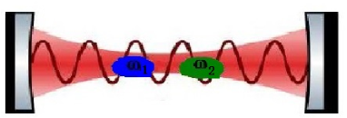
Fig. 1: Schematic diagram for two ensembles of ultracold atoms (blue and green) with transition frequencies $\omega_{1}$, $\omega_{2}$ in an optical cavity of frequency $\omega$.

We consider two ensembles of ultracold atoms, which are coupled simultaneously to an optical cavity mode of frequency $\omega$ as depicted in Fig. 1. Effective Hamiltonian of the system has the form [77] of two-component DM in the unit convention $\hbar=1$,

$$H = \omega a^{{\dagger}}a+\sum_{l=1,2}\omega_{l}J_{lz}$$

$$+\sum_{l=1,2}\frac{g_{l}}{\sqrt{N_{l}}}\left(a^{{\dagger}}+a\right)\left(J_{l+}+J_{l-}\right).$$

Where $J_{lz}$ $(J_{l\pm}=J_{lx}\pm iJ_{ly},\quad l=1,2)$ is the collective pseudospin operator with spin quantum-number $s_{l}$ $=N_{l}/2$. $N_{l}$ denotes the atom number of $l$-th component and $\omega_{l}$ is the atomic frequency. $a^{{\dagger}}\left(a\right)$ is the photon creation (annihilation) operator and $g_{l}$ is the atom-field coupling strength.

3 Spin coherent-state variational method

In this paper we provide analytic solutions for the macroscopic quantum state (MQS) for the spin-boson system in terms of the recently developed spin coherent variational method [78, 79, 48, 73]. The meaning of MQS in the present paper is that the variational wave function is considered as a product of boson and spin coherent states seen in the followings. We begin with the partial average of the system Hamiltonian in the trial wave function $\left|\alpha\right\rangle$, which is assumed as the boson coherent state of cavity mode such that $a\left|\alpha\right\rangle=\alpha\left|\alpha\right\rangle$. After the average in the boson coherent state we obtain an effective Hamiltonian of the pseudospin operators only,

$$H_{sp}\left(\alpha\right)=\left\langle\alpha\right|H\left|\alpha\right\rangle=\omega\alpha^{\ast}\alpha+\sum_{l=1,2}\omega_{l}J_{lz}+\sum_{l=1,2}\frac{g_{l}}{\sqrt{N_{l}}}\left(\alpha^{\ast}+\alpha\right)\left(J_{l+}+J_{l-}\right),$$ (1)

which is going to be diagonalized in terms of spin coherent-state transformation. A spin coherent state can be generated from the maximum Dicke states $\left|s,\pm s\right\rangle$ $(J_{z}$ $\left|s,\pm s\right\rangle=\pm s\left|s,\pm s\right\rangle$) with a spin coherent-state transformation [74, 80]. For the $l$-th component pseudospin operator we have two orthogonal coherent states defined by

$$\left|\pm\mathbf{n}_{l}\right\rangle=R(\mathbf{n}_{l})\left|s,\pm s\right\rangle_{l},$$

which are called north- and south- pole gauges respectively. As a matter of fact the spin coherent states are actually the eigenstates of the spin projection operator $\mathbf{J}_{l}\cdot\mathbf{n}_{l}\left|\pm\mathbf{n}_{l}\right\rangle=\pm j\left|\pm\mathbf{n}_{l}\right\rangle$, where $\mathbf{n}_{l}=\left(\sin\theta_{l}\cos\varphi_{l},\sin\theta_{l}\sin\varphi_{l},\cos\theta_{l}\right)$ is the unit vector with the directional angles $\theta_{l}$ and $\varphi_{l}$. In the spin coherent states the spin operators satisfy the minimum uncertainty relation, for example, $\Delta J_{+}\Delta J_{-}=\left\langle J_{z}\right\rangle/2$ so that $\left|\pm\mathbf{n}\right\rangle$ are called the MQSs. The unitary operator is explicitly given by

$$R(\mathbf{n}_{l})=e^{\frac{\theta_{l}}{2}(J_{l+}Je^{-i\varphi_{l}}-J_{l-}e^{i\varphi_{l}})}.$$ (2)

Since pseudospin operators for two components of atoms commute each other, the entire trail-wave-function is the direct product of two-component spin coherent states

$$|\psi_{s}\rangle=\left|\pm\mathbf{n}_{1}\right\rangle\left|\pm\mathbf{n}_{2}\right\rangle,$$

which is required to be the energy eigenstate of  the effective Hamiltonian of pseudospin operator such that

$$H_{sp}\left(\alpha\right)\left|\psi_{s}\right\rangle=E\left(\alpha\right)\left|\psi_{s}\right\rangle.$$ (3)

Where

$$|\psi_{s}\rangle=U\left|\pm s\right\rangle_{1}\left|\pm s\right\rangle_{2},$$ (4)

with

$$U=R(\mathbf{n}_{1})R(\mathbf{n}_{2}),$$

being the total unitary operator of spin coherent-state transformation. It is a key point to take into account of both spin coherent states $\left|\pm\mathbf{n}\right\rangle$ for revealing the multi-stable MQSs. Applying the unitary transformation $U^{{\dagger}}=R^{{\dagger}}(\mathbf{n}_{2})R^{{\dagger}}(\mathbf{n}_{1})$ to the energy eigenequation Eq. (3) we have

$$\widetilde{H}_{sp}\left(\alpha\right)\left|\pm s\right\rangle_{1}\left|\pm s\right\rangle_{2}=E\left(\alpha\right)\left|\pm s\right\rangle_{1}\left|\pm s\right\rangle_{2},$$

where

$$\widetilde{H}_{sp}\left(\alpha\right)=U^{{\dagger}}H_{sp}\left(\alpha\right)U.$$

Under the spin coherent-state transformation the spin operators $J_{lz}$, $J_{l+}$, $J_{l-}$ ($l=1$, $2$) become [80]

$$\widetilde{J}_{lz} = J_{lz}\cos\theta_{l}+\frac{1}{2}\sin\theta_{l}\left(J_{l+}e^{-i\varphi_{l}}+J_{l-}e^{i\varphi_{l}}\right),$$

$$\widetilde{J}_{l+} = J_{l+}\cos^{2}\frac{\theta_{l}}{2}-J_{l-}e^{2i\varphi_{l}}\sin^{2}\frac{\theta_{l}}{2}-J_{lz}e^{i\varphi_{l}}\sin\theta_{l},$$

$$\widetilde{J}_{l-} = J_{l-}\cos^{2}\frac{\theta_{l}}{2}-J_{l+}e^{-2i\varphi_{l}}\sin^{2}\frac{\theta_{l}}{2}-J_{lz}e^{-i\varphi_{l}}\sin\varphi_{l}.$$ (5)

Then the effective spin Hamiltonian can be diagonalized under the conditions

$$\frac{\omega_{l}}{2}e^{-i\varphi_{l}}\sin\theta_{l}+\widetilde{g}_{l\alpha}\left(\cos^{2}\frac{\theta_{l}}{2}-e^{-2i\varphi_{l}}\sin^{2}\frac{\theta_{l}}{2}\right)=0,$$

$$\frac{\omega_{1}}{2}e^{i\varphi_{l}}\sin\theta_{l}+\widetilde{g}_{l\alpha}\left(\cos^{2}\frac{\theta_{l}}{2}-e^{2i\varphi_{l}}\sin^{2}\frac{\theta_{l}}{2}\right)=0,$$ (6)

from which the angle parameters $\theta_{l}$, $\varphi_{l}$ are determined in principle. Thus we obtain the energy function

$$E\left(\alpha\right)=\omega\left|\alpha\right|^{2}\pm\sum_{l=1,2}\frac{N_{l}}{2}A_{l}\left(\alpha,\theta_{l},\varphi_{l}\right),$$

where

$$A_{l}\left(\alpha,\theta_{l},\varphi_{l}\right)=\omega_{l}\cos\theta_{l}-\widetilde{g}_{l\alpha}\left(e^{i\varphi_{l}}+e^{-i\varphi_{l}}\right)\sin\theta_{l},$$

with $\widetilde{g}_{l\alpha}=\frac{g_{l}}{\sqrt{N_{l}}}\left(\alpha^{\ast}+\alpha\right)$. The total trial-wave-function is

$$\left|\psi\right\rangle=\left|\alpha\right\rangle\left|\psi_{s}\right\rangle,$$ (7)

and corresponding energies are found as local minima of the energy function $E\left(\alpha\right)$, in which the complex eigenvalue of boson coherent state is parametrized as

$$\alpha=\gamma e^{i\phi}.$$

By solving the Eq. (6) and eliminating the angle parameters $\theta_{l},\varphi_{l},\phi$ we derive the scaled-energy as a function of one variational-parameter $\gamma$ only

$$\frac{E}{\omega}\left(\gamma\right)=\gamma^{2}\pm\sum_{l=1,2}\frac{N_{l}}{2}\sqrt{(\frac{\omega_{l}}{\omega})^{2}+\frac{16\gamma^{2}}{N_{l}}(\frac{g_{l}}{\omega})^{2}}.$$ (8)

The local minima of energy function Eq. (8) can be determined in terms of the variation with respect to the parameter $\gamma$.

4 Multi-stable states and phase diagram

In our formalism both the normal ($\Downarrow$) and inverted ($\Uparrow)$ pseudospin states [68, 75] are taken into account to reveal the multiple stable states. Thus there exist four combinations of two-spin states labeled by $\downarrow\downarrow$ (both normal spins), $\uparrow\uparrow$ (both inverted spins), $\downarrow\uparrow$ and $\uparrow\downarrow$ (first-spin normal, second-spin inverted and vas versa). For the configuration of both normal spins the dimensionless energy is

$$\frac{E_{\downarrow\downarrow}\left(\gamma\right)}{\omega}=\gamma^{2}-\sum_{l=1,2}\frac{N_{l}}{2}\sqrt{(\frac{\omega_{l}}{\omega})^{2}+\frac{16\gamma^{2}}{N_{l}}(\frac{g_{l}}{\omega})^{2}}.$$

In the following evaluations we assume the equal atom numbers for the two components that $N_{1}=N_{2}=N/2$. The atomic frequencies are parametrized according to the cavity frequency $\omega$ and atom-field detuning $\Delta$

$$\omega_{1}=\omega-\Delta,\omega_{2}=\omega+\Delta.$$ (9)

The ground-state is obtained from the variation of average energy

$$\varepsilon_{\downarrow\downarrow}=\frac{E_{\downarrow\downarrow}\left(\gamma\right)}{N\omega}$$

with respect to the variational parameter $\gamma$. The energy extremum condition is found as

$$\frac{\partial\varepsilon_{\downarrow\downarrow}}{\partial\gamma}=2\gamma_{\downarrow\downarrow}p_{\downarrow\downarrow}(\gamma_{\downarrow\downarrow})=0,$$ (10)

where

$$p_{\downarrow\downarrow}(\gamma_{\downarrow\downarrow})=1-\sum_{l=1,2}\frac{4g_{l}^{2}}{\omega^{2}F_{l}(\gamma_{\downarrow\downarrow})},$$

and

$$F_{l}(\gamma_{\downarrow\downarrow})=\sqrt{(\frac{\omega_{l}}{\omega})^{2}+32(\frac{g_{l}}{\omega})^{2}\frac{\gamma_{\downarrow\downarrow}^{2}}{N}}.$$

The extremum condition Eq. (10) possesses always a zero photon-number solution $\gamma_{\downarrow\downarrow}=0$, which is stable if the second-order derivative of energy function,

$$\frac{\partial^{2}(\varepsilon_{\downarrow\downarrow}(\gamma_{\downarrow\downarrow}^{2}=0)}{\partial\gamma^{2}}=2\left[1-\frac{4}{\omega}\left(\frac{g_{1}^{2}}{\omega_{1}}+\frac{g_{2}^{2}}{\omega_{2}}\right)\right],$$

is positive. Therefore a phase boundary is determined from $\partial^{2}(\varepsilon_{\downarrow\downarrow}(\gamma_{\downarrow\downarrow}^{2}=0)/\partial\gamma^{2}=0$, which gives rise to the relation of two critical coupling values

$$\frac{g_{1,c}^{2}}{\omega_{1}}\mathbf{+}\frac{g_{2,c}^{2}}{\omega_{2}}\mathbf{=}\frac{\omega}{4}.$$

When

$$\frac{g_{1}^{2}}{\omega_{1}}+\frac{g_{2}^{2}}{\omega_{2}}<\frac{\omega}{4},$$ (11)

we have a stable zero photon-number solution, which we call the NP denoted by $N_{\downarrow\downarrow}$. The energy function for the configuration $\downarrow\uparrow$ is

$$\varepsilon_{{}_{\downarrow\uparrow}}=\frac{\gamma^{2}}{N}-\frac{1}{4}[F_{1}(\gamma_{\downarrow\uparrow})-F_{2}(\gamma_{\downarrow\uparrow})]$$

The energy extremum condition $\partial\varepsilon_{{}_{\downarrow\uparrow}}/\partial\gamma=2\gamma_{\downarrow\uparrow}p_{\downarrow\uparrow}(\gamma_{\downarrow\uparrow})=0$ with

$$p_{\downarrow\uparrow}(\gamma_{\downarrow\uparrow})=1-\frac{4}{\omega^{2}}\left[\frac{g_{1}^{2}}{F_{1}(\gamma_{\downarrow\uparrow})}-\frac{g_{2}^{2}}{F_{2}(\gamma_{\downarrow\uparrow})}\right],$$

has the zero photon-number solution, which is stable when the second-order derivative

$$\frac{\partial^{2}\left(\varepsilon_{{}_{\downarrow\uparrow}}(\gamma_{\downarrow\uparrow}^{2}=0)\right)}{\partial\gamma^{2}}=\frac{2}{N}\left[1-\frac{4}{\omega}\left(\frac{g_{1}^{2}}{\omega_{1}}-\frac{g_{2}^{2}}{\omega_{2}}\right)\right]$$

is positive. Thus we have the NP (denoted by $N_{\downarrow\uparrow}$ ) region when

$$\frac{g_{1}^{2}}{\omega_{1}}-\frac{g_{2}^{2}}{\omega_{2}}<\frac{\omega}{4}.$$ (12)

Correspondingly for the configuration $\uparrow\downarrow$ the energy function is

$$\varepsilon_{{}_{\uparrow\downarrow}}=\frac{\gamma^{2}}{N}+\frac{1}{4}\left[F_{1}(\gamma)-F_{2}(\gamma)\right].$$

The energy extremum condition is $\partial\varepsilon_{{}_{\uparrow\downarrow}}/\partial\gamma=\gamma_{\uparrow\downarrow}p_{\uparrow\downarrow}(\gamma_{\uparrow\downarrow})=0$ with

$$p_{\uparrow\downarrow}(\gamma_{\uparrow\downarrow})=1+\frac{4}{\omega^{2}}\left(\frac{g_{1}^{2}}{F_{1}(\gamma_{\uparrow\downarrow})}-\frac{g_{2}^{2}}{F_{2}(\gamma_{\uparrow\downarrow})}\right).$$

Again the stable zero photon-number solution denoted by $N_{\uparrow\downarrow}$ requires

$$\frac{g_{2}^{2}}{\omega_{2}}-\frac{g_{1}^{2}}{\omega_{1}}<\frac{\omega}{4}.$$ (13)

The energy function for the configuration $\uparrow\uparrow$ is

$$\varepsilon_{\uparrow\uparrow}=\frac{E_{\uparrow\uparrow}\left(\gamma\right)}{\omega N}=\frac{\gamma^{2}}{N}+\frac{1}{4}\sum_{l=1,2}F_{l}(\gamma).$$

The extremum condition is

$$\frac{\partial(\varepsilon_{\uparrow\uparrow})}{\partial\gamma}=2\gamma_{\uparrow\uparrow}p_{\uparrow\uparrow}(\gamma_{\uparrow\uparrow})=0,$$

with

$$p_{\uparrow\uparrow}(\gamma_{\uparrow\uparrow})=1+\sum_{l=1,2}\frac{4g_{l}^{2}}{\omega^{2}F_{l}(\gamma_{\uparrow\uparrow})}.$$

The zero photon-number solution is stable denoted by $N_{\uparrow\uparrow}$ since the second-order derivative

$$\frac{\partial^{2}\varepsilon_{\uparrow\uparrow}\left(\gamma_{\uparrow\uparrow}^{2}=0\right)}{\partial\gamma^{2}}=\frac{2}{N}\left[1+\frac{4}{\omega}\left(\frac{g_{1}^{2}}{\omega_{1}}+\frac{g_{2}^{2}}{\omega_{2}}\right)\right]>0,$$

is always positive. The nonzero-photon solution can be obtained from the extremum condition.

$$p_{k}(\gamma_{sk})=0$$ (14)

for the four configurations $k=\downarrow\downarrow,\downarrow\uparrow,\uparrow\downarrow,\uparrow\uparrow$. The extremum condition Eq. (14) is able to be solved numerically. We display in Fig. 2(a) the stable nonzero photon solutions $\gamma_{sk}$, which are called the superradiant states, and the corresponding energies $\varepsilon(\gamma_{sk})$ as shown in Fig. 2(b) for $k=\downarrow\downarrow$ (black line)$,\downarrow\uparrow$ (olive line)$,\uparrow\downarrow$ (blue line) respectively. For the dimensionless coupling $g_{2}/\omega=0.2$ [Figs. 2(a1) and 2(b1)] both solutions $\gamma_{s\downarrow\downarrow}$ and $\gamma_{s\downarrow\uparrow}$ of the extremum equation are stable with a positive sloop [Fig. 2(a1)], namely a positive second-order derivative of the energy function with respect the variation parameter $\gamma$. The corresponding energies are local minima [Fig. 2(b1)]. $\gamma_{s\downarrow\uparrow}$ indicates the solution of stimulated radiation from the state of atomic population inversion for the second-component of atoms. Increasing the coupling strength to $g_{2}/\omega=0.4$ [Figs. 2(a2) and 2(b2)] and $0.7$ we have only one stable solution $\gamma_{s\downarrow\downarrow}$. While the two stable solutions appear again for $g_{2}/\omega=0.9$ [Figs. 2(a4) and 2(b4)]. It is interesting to see a fact that the the stimulated radiation becomes the first-component of atoms i.e. $\gamma_{s\uparrow\downarrow}$. The superradiant states are denoted respectively by $S_{\downarrow\downarrow}$, $S_{\uparrow\downarrow}$ and $S_{\downarrow\uparrow}$ in the following phase diagrams.

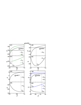
Fig. 2: Graphical solutions of the extremum equation $p_{k}(\gamma_{sk})=0$ for $k=\downarrow\downarrow$ (black line), $k_{\downarrow\uparrow}$ (olive line), and $k=\uparrow\downarrow$ (blue line) with $g_{1}/\omega=0.6$ and $g_{2}$/$\omega=0.2$ (a1), $0.4$ (a2), $0.7$ (a3), $0.9$ (a4). The corresponding average energy curves $\varepsilon$ are plotted in the lower panel (b1-b4). $\bar{\gamma}^{2}$ $=\gamma^{2}/N$ denotes the mean photon number.

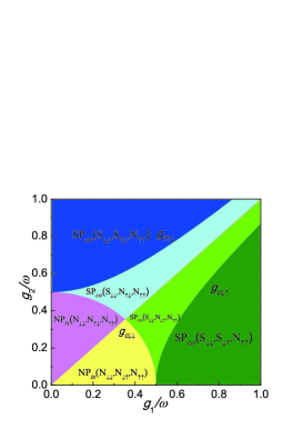
Fig. 3: Phase diagram in the resonance condition $\omega_{1}=\omega_{2}=\omega$. The notations $NP_{ts}\left(N_{\downarrow\downarrow},N_{\uparrow\downarrow}\mathbf{,}N_{\downarrow\downarrow}\right)$ and $NP_{ts}\left(N_{\downarrow\downarrow},N_{\downarrow\uparrow}\mathbf{,}N_{\downarrow\downarrow}\right)$ mean the NP with triple states, in which $N_{\downarrow\downarrow}$ is the ground state. $SP_{co}\left(S_{\downarrow\downarrow},N_{\uparrow\downarrow}\mathbf{,}N_{\uparrow\uparrow}\right)$ [ $SP_{co}\left(S_{\downarrow\downarrow},N_{\downarrow\uparrow}\mathbf{,}N_{\uparrow\uparrow}\right)$] means the SP characterized by the ground state $S_{\downarrow\downarrow}$, which coexists with $N_{\uparrow\downarrow}$ ( $N_{\downarrow\uparrow}$) and $N_{\uparrow\uparrow}$. $SP_{co}\left(S_{\downarrow\downarrow},S_{\uparrow\downarrow}\mathbf{,}N_{\uparrow\uparrow}\right)$ [ $SP_{co}\left(S_{\downarrow\downarrow},S_{\downarrow\uparrow}\mathbf{,}N_{\uparrow\uparrow}\right)$] is also the coexisting SP, in which the first excited-state is a superradiant state  $S_{\uparrow\downarrow}$ ( $S_{\downarrow\uparrow}$) .

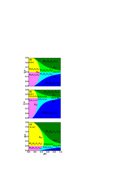
Fig. 4: Phase diagram in $g$-$\Delta$ space with the atom-photon coupling parameter $\delta=0$ (a), $\delta=0.5$ (b), and $\delta=-0.5$ (c).  The boundary line, which separates the regions with different first-excited-states ($N_{\downarrow\uparrow}$, $S_{\downarrow\uparrow}$ and $N_{\uparrow\downarrow}$, $S_{\uparrow\downarrow}$), moves upward and downward respectively for $\delta=0.5$ (b) , $-0.5$ (c).

The new observation with the spin coherent-state variational-method is that besides the ground states we also obtained the stable MQSs of higher energies. Fig. 3 depicts the phase diagram in $g_{1}$-$g_{2}$ plane with the resonance condition $\omega_{1}=\omega_{2}=\omega$. The phase boundaries $g_{c\downarrow\downarrow}$ $g_{c\downarrow\uparrow}$ $g_{c\uparrow\downarrow}$ are determined from the following three relations respectively

$$\mathbf{\ }g_{2}=\frac{1}{2}\sqrt{1-\left(\frac{2g_{1}}{\omega}\right)^{2}},$$

$$g_{2}=\frac{1}{2}\sqrt{\left(\frac{2g_{1}}{\omega}\right)^{2}+1},$$

$$g_{2}=\frac{1}{2}\sqrt{\left(\frac{2g_{1}}{\omega}\right)^{2}-1}.$$

In the region denoted by $NP_{ts}$ (bounded by the critical line $g_{c\downarrow\downarrow}$) there exist triple zero-photon states, in which $N_{\downarrow\downarrow}$ with lowest energy is the ground state. This region is separated into two areas (pink and yellow) with only one state difference that the state $N_{\downarrow\uparrow}$ in one area is replaced by $N_{\uparrow\downarrow}$ in the other. We see the simultaneous spin-flip from the state $N_{\downarrow\uparrow}$ to $N_{\uparrow\downarrow}$ by adjusting the ratio of two coupling constants from $g_{2}/g_{1}<1$ (yellow region) to $g_{2}/g_{1}>1$ (pink region). The notation, for example, $SP_{co}(S_{\downarrow\downarrow},N_{\uparrow\downarrow},N_{\uparrow\uparrow})$ (cyan area) means the SP region characterized by the superradiant ground-state $S_{\downarrow\downarrow}$ coexisting with the first ($N_{\uparrow\downarrow}$) and second ($N_{\uparrow\uparrow}$) excited states of zero photons). The phase diagram is symmetric with respect to the line $g_{2}/g_{1}=1$, which separates the SP region to two areas. Below the symmetric line (green area) only the first excited state is changed to $N_{\downarrow\uparrow}$ by the coupling-variation induced spin flip. The critical line $g_{c\uparrow\downarrow}$ is a boundary, above which the first excited state becomes surperradiant state $S_{\uparrow\downarrow}$ (cyan region) in the upper area of the symmetric line. While $g_{c\downarrow\uparrow}$ is the corresponding boundary for the first excited states $N_{\downarrow\uparrow}$ and $S_{\downarrow\uparrow}$ (olive area). The superradiant states $S_{\uparrow\downarrow}$, $S_{\downarrow\uparrow}$, which are new observation for the two-component BECs, are seen to be the stimulated radiation from the higher-energy atomic levels. The stable population inversion state $N_{\uparrow\uparrow}$ for both components exists in the whole region. The multi-stable MQSs observed in this paper agree with the dynamic study of nonequilibrium QPTs [75, 68].

We now consider the phase diagram for the atom-field detuning $\omega_{1}=\omega-\Delta$ and $\omega_{2}=\omega+\Delta$ with $\Delta\in\left[-0.9,0.9\right]$ and the atom-field coupling imbalance parameter $\delta$ given by

$$g_{1}=g,g_{2}=(1+\delta)g.$$ (15)

Substituting atom-field coupling Eq. (15) into the corresponding ground-state energy function we obtain the phase diagram of $g$-$\Delta$ space displayed in Fig. 4 for the imbalance parameter $\delta=0$ [Fig. 4(a)], $0.5$ [Fig. 4(b)], $-0.5$ [Fig. 4(c)]. The phase boundary line $g_{c\downarrow\downarrow}$ for the normal state $N_{\downarrow\downarrow}$ is found from Eq. (11)

$$g_{c_{\downarrow\downarrow}}=\frac{1}{2}\sqrt{\frac{(\omega^{2}-\Delta^{2})}{\omega\left[2\omega+(\omega-\Delta)\left(2\delta+\delta^{2}\right)\right]}},$$ (16)

The phase diagram for $\delta=0$ as depicted in Fig. 4(a) is symmetric with respect to the horizontal line $\Delta=0$. The triple-state NP region denoted by $NP_{ts}(N_{\downarrow\downarrow},N_{\downarrow\uparrow},N_{\uparrow\uparrow}\mathbf{)}$ (yellow) and $NP_{ts}(N_{\downarrow\downarrow},N_{\uparrow\downarrow},N_{\uparrow\uparrow}\mathbf{)}$ (pink) is located on the left-hand side of the critical line $g_{c\downarrow\downarrow}$, which shifts towards the lower value direction of the atom-field coupling $g$ [21, 68] with the increase of absolute value of detuning $\left|\Delta\right|$ seen from Fig. 4(a). $SP_{co}\left(S_{\downarrow\downarrow},N_{\downarrow\uparrow}\mathbf{,}N_{\uparrow\uparrow}\right)$ (green region) and $SP_{co}\left(S_{\downarrow\downarrow},N_{\uparrow\downarrow}\mathbf{,}N_{\uparrow\uparrow}\right)$ (cyan) denote the SP characterized by the ground-state $S_{\downarrow\downarrow}$ coexisting with the normal states $N_{\downarrow\uparrow}$, $N_{\uparrow\downarrow}$ and $N_{\uparrow\uparrow}$ respectively. The QPT from the NP of ground-state $N_{\downarrow\downarrow}$ to the SP of ground-state $S_{\downarrow\downarrow}$ by the variation of atom-field coupling $g$ is the standard DM type for the fixed atom-field detuning $\Delta$. The phase boundary lines $g_{c\downarrow\uparrow}$, $g_{c\uparrow\downarrow}$, which separate the states $S_{\downarrow\uparrow}$ and $S_{\uparrow\downarrow}$, are respectively determined from Eqs. (12, 13) 

$$g_{c\downarrow\uparrow}=\frac{1}{2}\sqrt{\frac{(\omega^{2}-\Delta^{2})}{\omega\left[(\omega+\Delta)-(\omega-\Delta)(1+\delta)^{2}\right]}}=\frac{1}{2}\sqrt{\frac{(\omega^{2}-\Delta^{2})}{\omega\left[2\Delta-(\omega-\Delta)\left(2\delta+\delta^{2}\right)\right]}},$$ (17)

and

$$g_{c\uparrow\downarrow}=\frac{1}{2}\sqrt{\frac{(\omega^{2}-\Delta^{2})}{\omega\left[(\omega-\Delta)(1+\delta)^{2}-(\omega+\Delta)\right]}}=\frac{1}{2}\sqrt{\frac{(\omega^{2}-\Delta^{2})}{\omega\left[(\omega-\Delta)\left(2\delta+\delta^{2}\right)-2\Delta\right]}}.$$ (18)

The superradiant region denoted by $SP_{co}\left(S_{\downarrow\downarrow},S_{\downarrow\uparrow}\mathbf{,}N_{\uparrow\uparrow}\right)$ (olive area) is above the the critical line $g_{c\downarrow\uparrow}$, while $SP_{co}\left(S_{\downarrow\downarrow},S_{\uparrow\downarrow}\mathbf{,}N_{\uparrow\uparrow}\right)$ (blue) is located below the critical line $g_{c\uparrow\downarrow}$. We see that the second excited-state varies from the normal state $N_{\downarrow\uparrow}$ to the superradiant state $S_{\downarrow\uparrow}$ by the increase of detuning $\Delta$. The difference of upper and lower half-plane of the phase diagram is made only by the first excited-states $N_{\downarrow\uparrow}$, $S_{\downarrow\uparrow}$ and $N_{\uparrow\downarrow}$, $S_{\uparrow\downarrow}$ with the interchange of spin polarizations between two components. This boundary line, which separates the regions with different first excited-states, moves upward and downward respectively for $\delta=0.5$ [Fig. 4(b)], $-0.5$ [Fig. 4(c)].

5 Mean photon number, atomic population and average energy from viewpoint of phase transition

The mean photon numbers in the states $N_{\downarrow\downarrow}$ and $S_{\downarrow\downarrow}$ can be evaluated directly from the average of photon number-operator in the corresponding wave functions $|\psi\rangle=\left|\alpha\right\rangle\left|\psi_{s}\right\rangle$ in Eq. (7) with spin-state $|\psi_{s}(-s,-s)\rangle=U\left|-s\right\rangle_{1}\left|-s\right\rangle_{2}$ given in Eq. (4). The result is obviously

$$n_{p}(\downarrow\downarrow)=\frac{\left\langle\alpha|a^{{\dagger}}a|\alpha\right\rangle}{N}=\left\{\begin{array}[]{r}0,\qquad\ g<g_{c\downarrow\downarrow},\\ \frac{\gamma_{\downarrow\downarrow}^{2}}{N},\qquad g>g_{c\downarrow\downarrow}.\end{array}\right..$$

While the atomic population imbalance becomes

$$\Delta n_{a}\left(\downarrow\downarrow\right)=\frac{\left\langle\psi_{s}(-s,-s)|(J_{1z}+J_{2z})|\psi_{s}(-s,-s)\right\rangle}{N}=-\frac{1}{4}\sum_{l=1,2}\frac{\omega_{l}}{\omega F_{l}(\gamma_{\downarrow\downarrow})},$$

which reduces to the well-known standard Dicke-model value

$$\Delta n_{a}(\downarrow\downarrow)=-\frac{1}{2},$$

at the critical line $g_{c\downarrow\downarrow}$ and also the NP state $N_{\downarrow\downarrow}$. The average energy in ground states $N_{\downarrow\downarrow}$ and $S_{\downarrow\downarrow}$ is given by

$$\varepsilon_{{}_{\downarrow\downarrow}}=\left\{\begin{array}[]{r}-0.5,g<g_{c\downarrow\downarrow},\\ \frac{\gamma_{\downarrow\downarrow}^{2}}{N}-\frac{1}{4}\sum\limits_{l=1,2}F_{l}(\gamma_{\downarrow\downarrow}),g>g_{c\downarrow\downarrow}.\end{array}\right..$$

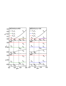
Fig. 5: Variations of the average photon number $n_{p}$ (a), atom population imbalance $\Delta n_{a}$ (b), and average energy $\varepsilon$ (c) with respect to the coupling constant $g=$ $g_{1}=g_{2}$ in the atom-field frequency detuning $\Delta=0.6$ (1) and $\Delta=-0.6$ (2).

For the states $N_{k}$ and $S_{k}$ with opposite spin-polarizations $k=\downarrow\uparrow$,$\uparrow\downarrow$ the average photon number is

$$n_{p}(N_{k})=0;\qquad n_{p}(S_{k})=\frac{\gamma_{k}^{2}}{N}.$$

The atomic population imbalance becomes

$$\Delta n_{a}(N_{k})=0$$

for the zero-photon states $N_{k}$. While the atomic population imbalance for the superradiant states $S_{k}$ is seen to be

$$\Delta n_{a}(S_{\downarrow\uparrow})=\frac{1}{4\omega}\left[-\frac{\omega_{1}}{F_{1}(\gamma_{\downarrow\uparrow})}+\frac{\omega_{2}}{F_{2}(\gamma_{\downarrow\uparrow})}\right],$$

$$\Delta n_{a}(S_{\uparrow\downarrow})=\frac{1}{4\omega}\left[\frac{\omega_{1}}{F_{1}(\gamma_{\uparrow\downarrow})}-\frac{\omega_{2}}{F_{2}(\gamma_{\uparrow\downarrow})}\right].$$

The average energies $\varepsilon_{k}(S_{k})$ of the superradiant states $S_{k}$ for $k=\downarrow\uparrow$,$\uparrow\downarrow$ can be obtained from the energy functions with the corresponding solutions $\gamma_{k}$, which lead to $\varepsilon_{k}(N_{k})=0$. For the inverted-spin state of zero photon the atomic population imbalance is $\Delta n_{a}(N_{\uparrow\uparrow})=0.5$ and the average energy is found as

$$\varepsilon(N_{\uparrow\uparrow})=\frac{1}{4\omega}(\omega_{1}+\omega_{2}).$$

The stable nonzero-photon state does not exists for this configuration of both inverted spins. The average photon number $n_{p}$, atomic population imbalance $\Delta n_{a}$, and the average energy $\varepsilon$ are plotted in Fig. 5 as functions of the atom-field coupling strength $g$ in the red and blue detuning $\Delta=\pm 0.6$ with $\delta=0$. Below the critical point $g_{c\downarrow\downarrow}$ we have triple stable (zero-photon) states denoted by $NP_{ts}\left(N_{\downarrow\downarrow},N_{\downarrow\uparrow}\mathbf{,}N_{\uparrow\uparrow}\right)$ [or $NP_{ts}\left(N_{\downarrow\downarrow},N_{\uparrow\downarrow}\mathbf{,}N_{\uparrow\uparrow}\right)$], in which $N_{\downarrow\downarrow}$ (black line) is the ground state with lowest energy. Between the critical points $g_{c\downarrow\downarrow}$ and $g_{c\downarrow\uparrow}$ (or $g_{c\uparrow\downarrow}$) the superradiant ground-state $S_{\downarrow\downarrow}$ (black line) coexists with the states $N_{\downarrow\uparrow}$ [olive lines in Figs. 5(a1)-5(c1)], or $N_{\uparrow\downarrow}$ [blue lines in Figs. 5(a2)-5(c2)], and $N_{\uparrow\uparrow}$ (red lines). The QPT from the NP ($N_{\downarrow\downarrow}$) to the SP ($S_{\downarrow\downarrow}$) is the standard DM type, which takes place at the critical point $g_{c\downarrow\downarrow}$. From Fig. 5(c1) we see that the states  $N_{\downarrow\uparrow}$ and $S_{\downarrow\uparrow}$ (olive lines) of opposite spin-polarizations are the first excited-states in the case $\Delta=6$. While the states $N_{\uparrow\downarrow}$ and $S_{\uparrow\downarrow}$ with interchange of the spin polarizations between two components become the first excited states seen from Fig. 5(c2) (blue lines) for the negative detuning $\Delta=-6$. We observe for the first time the phase transition at the critical point $g_{c\downarrow\uparrow}$ $(g_{c\uparrow\downarrow}$) from the normal state $N_{\downarrow\uparrow}$ ( $N_{\uparrow\downarrow}$) to the suprradiant state $S_{\downarrow\uparrow}$ ($S_{\uparrow\downarrow}$), which is the stimulated radiation from the collective states of atomic population inversion for one component of BECs seen from Figs. 5 and 6. The ground state does not change at the critical point $g_{c\downarrow\uparrow}$ (or $g_{c\uparrow\downarrow}$), which separates the normal state $N_{\downarrow\uparrow}$ (or $N_{\uparrow\downarrow}$) and the superradiant one $S_{\downarrow\uparrow}$ (or $S_{\uparrow\downarrow}$), which are the collective excited-states of the system. For the given frequency detuning $\Delta=\pm 0.6$ (Fig. 5) the critical points can be evaluated precisely for Eq. (16, 17, 18), $g_{c\downarrow\downarrow}=\sqrt{2}/5=0.2828$ and $g_{c\downarrow\uparrow}=g_{c\uparrow\downarrow}\mathbf{=}\sqrt{2/15}=0.365148$. The normal state $N_{\uparrow\uparrow}$ (red line) of atomic population inversion for both components does not involve in radiation process.

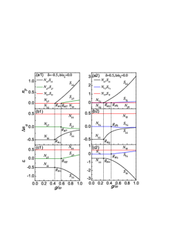
Fig. 6: The average photon number $n_{p}$ (a), atomic population $\Delta n_{a}$ (b), and average energy $\varepsilon$ (c) curves for the imbalance parameter $\delta=-0.5$ (1), $\delta=0.5$ (2) in the resonance condition $\Delta=0.0$. The stimulated radiation shifts from one component to the other by adjusting the relative coupling constants.

We display the variation curves of average photon-number $n_{p}$ as shown in Figs. 6(a1) and 6(a2), atom population imbalance $\Delta n_{a}$ as shown in Figs. 6(b1) and 6(b2), and energy $\varepsilon$ as depicted in Figs. 6(c1) and 6(c2) with respect the coupling constant $g$ for the imbalance parameter $\delta=\pm 0.5$ at the resonance condition $\Delta=0$. The QPT from normal state $N_{\downarrow\downarrow}$ to the superradiant state $S_{\downarrow\downarrow}$ takes place at the critical point $g_{c\downarrow\downarrow}=\sqrt{5}/5=0.447214$. In the case $\delta=-5$ as depicted in Figs. 6(a1)-6(c1), namely the second component has lower coupling value, an additional transition appears between the collective excited-states  $N_{\downarrow\uparrow}$ and $S_{\downarrow\uparrow}$ at the critical point $g_{c\downarrow\uparrow}=\sqrt{3}/3=0.577350$. This transition is from the normal state of atomic population inversion to the superradiant state for the second component realized from atom population imbalance and the energy in Figs. 5(b1) and 5(c1). By adjusting the imbalance parameter to $\delta=0.5$ as shown Figs. 6(a2)-6(c2), the transition becomes from $N_{\uparrow\downarrow}$ to $S_{\uparrow\downarrow}$ for the first component. The collective stimulated-radiation shifts to the first component, which has lower atom-field coupling than the second component in this case. The transition critical point is found as $g_{c\uparrow\downarrow}=\sqrt{5}/5=0.447214$.

6 Conclusion and discussion

In summary, multiple MQSs are derived analytically for two-component BECs in a single-mode cavity by means of the spin coherent-state variational method. The rich phase diagrams are presented with the variation of atom-field coupling imbalance between two components and the atom-field frequency detuning. Indeed the ground states display a typical Dicke-model QPT from the NP to SP for both components in the normal spin-states. When the atom-field coupling imbalance between two components increases the normal spin-state with relatively lower coupling-value flips to the inverted spin-state, the radiation from this state is the stimulated radiation from atomic population-inversion levels. The stimulated radiation can be also generated from manipulation of atom-field frequency detuning. In the specific cases when one of the coupling constants vanishes or two couplings are equal the ground-states and related QPT reduce to that of an ordinary Dicke model. The controllable stimulated radiation may have technical applications in the laser physics. The spin coherent-state variational method is a powerful tool in the study of macroscopic quantum properties for the atom-ensemble and cavity-field system, since it takes into account both the normal and inverted pseudospins, which result in multiple MQSs in agreement with the semiclassical dynamics of nonequilibrium QPT in the Dicke model [76]. In addition a one-parameter variational energy-function is able to be derived in this formalism, so that one can evaluate the second-order derivative to determine rigorously the local minima of energy functions in consistence with the numerical simulation [48, 77, 73, 75, 68].

Funding

This work was supported by the National Natural Science Foundation of China (Grant Nos. 11275118, 11404198, 91430109, 61505100), and the Scientific and Technological Innovation Programs of Higher Education Institutions in Shanxi Province (STIP) (Grant No. 2014102), and the Launch of the Scientific Research of Shanxi University (Grant No. 011151801004), and the National Fundamental Fund of Personnel Training (Grant No. J1103210). The natural science foundation of Shanxi Province(Grant No. 2015011008).