Droplet Ripening in Concentration Gradients

Abstract

Living cells use phase separation and concentration gradients to organize chemical compartments in space. Here, we present a theoretical study of droplet dynamics in gradient systems. We derive the corresponding growth law of droplets and find that droplets exhibit a drift velocity and position dependent growth. As a consequence, the dissolution boundary moves through the system, thereby segregating droplets to one end. We show that for steep enough gradients, the ripening leads to a transient arrest of droplet growth that is induced by an narrowing of the droplet size distribution.

1 Introduction: Droplet ripening in concentration gradients in biology

Living cells have to organize many molecules in space and time in order to build compartments which can perform certain biological functions. The formation of these compartments is often regulated by spatially heterogenous distributions of molecular species. An example is the polarized distribution of polarity proteins in the course of asymmetric cell division [1, 2, 3]. During asymmetric cell division, molecules of the cell cytoplasm are distributed unequally between both daughter cells [4, 5]. This can be studied in the first division of the fertilized egg of the roundworm C.elegans. RNA-protein aggregates called P-granules are segregated to the posterior side of the cell and are located in the posterior daughter cell after division. P-granules are liquid like droplets that form by phase separation from the cell cytoplasm [6, 1, 2, 3]. The segregation and ripening of P-granule droplets toward the posterior is driven by a concentration gradient of the protein Mex-5 that regulates droplet dynamics [6, 7, 8].

The ripening of drops guided by a concentration gradient of molecules that regulate phase separation fundamentally differs from classical Ostwald-ripening. In the case of Ostwald ripening, droplets are uniformly distributed throughout the system and the droplet size distribution broadens with time [9, 10, 11, 12]. If a concentration gradient of a regulator component is maintained, for example by sources and sinks [8], or via position-dependent reaction kinetics [13, 14], there is a broken symmetry generating a bias of droplet positions. Recently, droplet segregation in a concentration gradient has been discussed using a simplified model [7]. However, the dynamics of droplets ripening in a gradient of regulating molecules has not been explored (figure 1(a)).

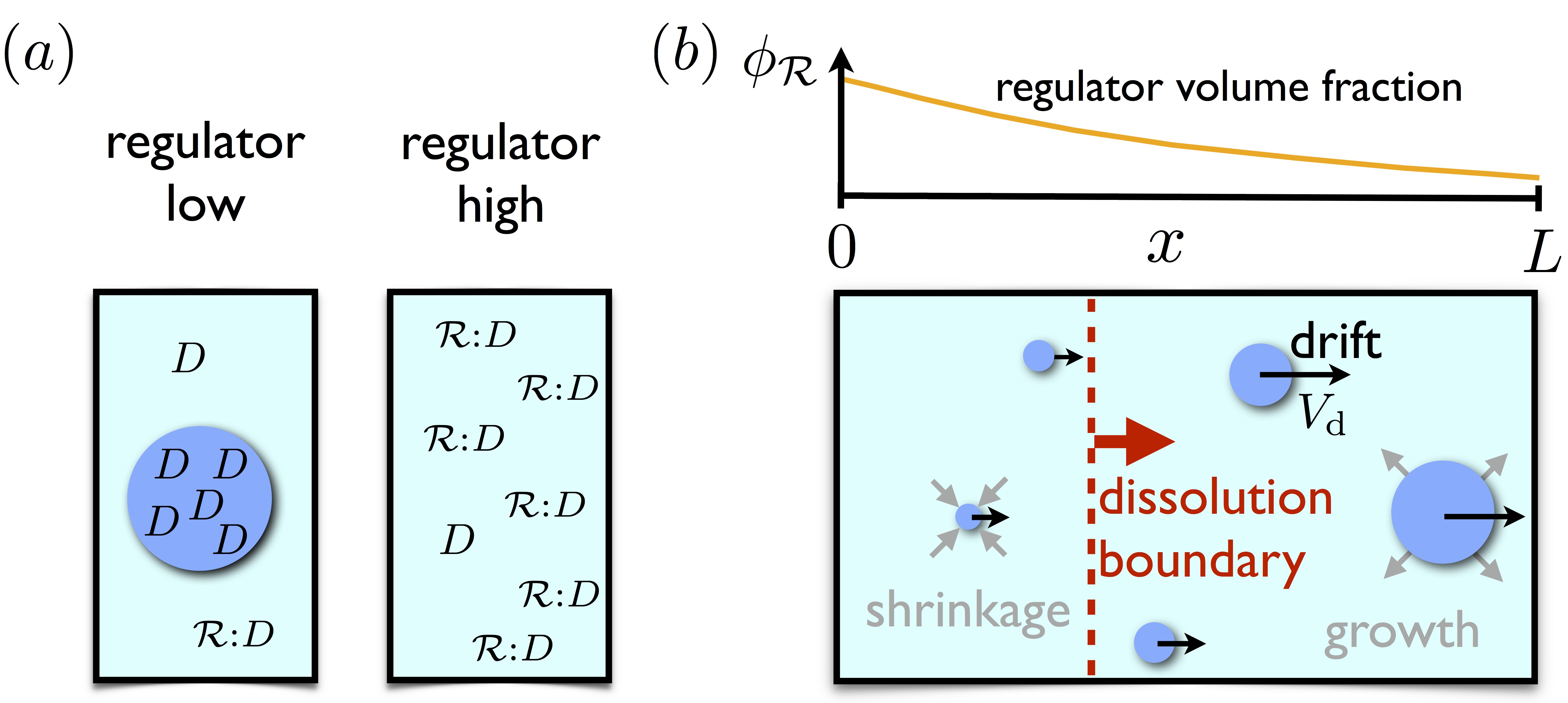
Figure 1: (a) Schematic representation of the regulation of droplet (blue dot) formation by a regulator $R$ which can bind to droplet material $D$ to form the product $\mathcal{R}$:${D}$. (b) Illustration of droplet ripening in a gradient of regulator volume fraction $\phi_{R}$ (orange). At each time point a boundary (red dashed) divides the system into domains of growth and shrinkage. This boundary moves to the right (red arrow) leaving a region of dissolving drops behind. Droplets drift (black arrows) with velocity $V_{\mathrm{d}}$.

In this paper we present a theoretical study of droplet ripening in a concentration gradient of a regulator that affects phase separation. Considering a simplified theory we extract generic physical features of droplet growth in the presence of concentration gradients. The generic features we study here are the spatially dependent, local equilibrium concentration and a spatially dependent actual concentration outside the droplets. If the distance between droplets is large, these features can be used to derive the generic laws of droplet ripening in concentrations gradients and thereby extend the classical theory for homogeneous systems [9, 10]. Our central finding is that a regulator gradient leads to a drift velocity and a position dependent growth of drops (figure 1(b)). As a consequence, a dissolution boundary moves through the system, leaving droplets only in a region close to one boundary of the system. Using numerical calculations supported by analytic estimates, we study the growth dynamics of droplets in a gradient. We discover that, surprisingly, ripening is not always faster in the case of steeper regulator gradients. Instead, a transient arrest of ripening is observed that results from a narrowing of the droplet size distribution. Our work shows that a regulator gradient induces a novel and rich ripening dynamics in droplet systems.

2 Local regulation of phase separation

We use a simplified model to discuss two component phase separation that is influenced by a regulator. We consider a system consisting of a solvent ${S}$, droplet material ${D}$ and a regulator $\mathcal{R}$ that can create together with the droplet material a bound state $\mathcal{R}$:${D}$. In this model the regulator does not take part in demixing but influences phase separation of ${D}$ and ${S}$. We describe demixing by a simplified Flory-Huggins type of free-energy density

$$f={k_{B}T}\bigg{[}\frac{\phi^{T}_{D}}{\nu_{{D}}}\ln{\phi^{T}_{D}}+\frac{\phi_{S}}{\nu_{{S}}}\ln{\phi_{S}}\bigg{]}+\mathcal{E}\,,$$ (1)

where $k_{B}$ is the Boltzmann constant, $T$ is temperature and $\phi^{T}_{D}$ and $\phi_{S}$ denote the total volume fraction of droplet material and solvent, respectively, with $\phi^{T}_{D}+\phi_{S}=1$. In equation (1) we neglect for simplicity the mixing entropy of the component $\phi_{\mathcal{R}:{D}}$. We only consider interactions between droplet material ${D}$ and solvent ${S}$ and the corresponding interaction energies are described by $\mathcal{E}$. These simplifications do not affect the qualitative feature of position dependent phase separation that we highlight in this work but are useful simplification for the discussion of the relevant physics. The molecular volumes $\nu_{i}$ connect volume fractions with concentrations $c_{i}$ by $\phi_{i}=\nu_{i}c_{i}$. The regulator influences phase separation by binding to droplet material,

$${D}+\mathcal{R}\rightleftharpoons\mathcal{R}:{D}\,.$$ (2)

Here we consider the case where the bound state $\mathcal{R}$:${D}$ does not phase separate from the solvent. The total volume fraction of droplet material is given by the sum of contributions of bound and free molecules, $\phi^{T}_{D}=\phi_{D}+\phi_{\mathcal{R}:{D}}$. The binding process between regulator and droplet material can be described by mass action with the equilibrium binding constant $K_{0}=c_{\mathcal{R}:{D}}/(c_{D}c_{\mathcal{R}})$. Using the simplification $\nu_{\mathcal{R}:{D}}=\nu_{D}$, we write $K_{0}=\phi_{\mathcal{R}:{D}}/(\phi_{D}c_{\mathcal{R}})$. The interaction energy is given by $\mathcal{E}={k_{B}T}\chi\,\phi_{D}\phi_{S}$, where $\chi$ is the interaction parameter. Expressing $\phi_{D}$ in terms of $\phi^{T}_{D}$ and considering a fast local equilibrium of the binding reaction we find

$$\mathcal{E}(\phi^{T}_{D},\phi_{S})={k_{B}T}\chi_{\mathrm{eff}}\,\phi^{T}_{D}\phi_{S}\,,$$ (3)

with

$$\chi_{\mathrm{eff}}=\chi\left(1-\frac{K\phi_{\mathcal{R}}}{1+K\phi_{\mathcal{R}}}\right)$$ (4)

and $K=K_{0}/\nu_{\mathcal{R}}$. The function $\chi_{\mathrm{eff}}$ describes the effective interaction between the solvent and the total droplet material which depends on the regulator. In the case of a vanishing regulator concentration, $\phi_{\mathcal{R}}=0$, equation (1) reduces to the original Flory-Huggins model for binary polymer blends [15] with an interaction parameter $\chi_{\mathrm{eff}}=\chi$. Increasing the concentration of the regulator leads to a decrease in the effective interaction parameter $\chi_{\mathrm{eff}}$. This decrease is more pronounced if the binding constant $K$ is larger, which amounts to more $\mathcal{R}$ being bound to ${D}$. Please note that only for large values of $\chi_{\mathrm{eff}}$ relative to the entropic terms in equation (1) demixing can occur (figure 2(a)).

3 Spatial organization of phase separation

To describe the spatial regulation of phase separation we consider a spatially inhomogeneous system that is locally at thermodynamic equilibrium such that at each position the local free energy is defined. Globally the system is maintained away from equilibrium by an imposed position dependent regulator gradient. For simplicity, we use a linear gradient along the $x$ direction, $\phi_{\mathcal{R}}(x)=\phi_{0}-m\cdot x$, with $x\in[0,L]$, where $L$ denotes the size of the system. We first look at a situation without droplets but with a possible spatial profile $\phi_{D}=\bar{\Phi}(x)$ of droplet material. Since the spatial concentration profile of the regulator $\phi_{\mathcal{R}}(x)$ is imposed, the effective interaction parameter $\chi_{\mathrm{eff}}(x)$ becomes a function of $x$. As the droplet material is also distributed in space, the concentration at each position $x$ corresponds to a point in the phase diagram. The linear range $x\in[0,L]$ then maps onto a line that is indicated in the phase diagram in figure 2(a). Using the phase diagram, we can determine the position $x_{\mathrm{d}}$ of the dissolution boundary, which separates the region $x<x_{\mathrm{d}}$ where the fluid mixes, from the region $x>x_{\mathrm{d}}$ in which droplets can form. For $x>x_{\mathrm{d}}$, we can then determine the local equilibrium volume fraction ${\Phi^{\mathrm{in}}_{\mathrm{eq}}}(x)$ of the droplet material inside and ${\Phi^{\mathrm{out}}_{\mathrm{eq}}}(x)$ outside of a potential droplet, which depend on position. For $\nu_{S}\gg\nu_{D}$, ${\Phi^{\mathrm{in}}_{\mathrm{eq}}}$ is approximately constant along $x$. As we will see below, choosing this simple limit allows us to focus on the concentration field outside of the droplet. The spatial distribution of the regulator and droplet material imply a spatially dependent supersaturation defined as

$$\epsilon(x)=\frac{\bar{\Phi}(x)}{{\Phi^{\mathrm{out}}_{\mathrm{eq}}}(x)}-1\,,$$ (5)

which is positive for $x>x_{\mathrm{d}}$. In the absence of droplets, the concentration field $\bar{\Phi}(x)$ evolves in time satisfying a diffusion equation. If droplets are nucleated, their dynamics of growth or shrinkage is guided by the local supersaturation $\epsilon(x)$ as well as ${\Phi^{\mathrm{in}}_{\mathrm{eq}}}$ and ${\Phi^{\mathrm{out}}_{\mathrm{eq}}}(x)$. This droplet dynamics then in turn also influences the concentration field $\bar{\Phi}(x)$.

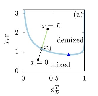
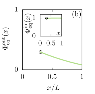
Figure 2: (a) Phase diagram. Interaction parameter $\chi_{\mathrm{eff}}$ as a function of the volume fraction of droplet material $\phi_{D}^{T}$. The binodal line (blue) and the critical point (triangle) are indicated. For a regulator concentration gradient, the positions $x$ in the system are mapped to a line (dashed/green line in the mixed/demixed region). At the position $x=x_{\mathrm{d}}$ this line crosses the binodal. (b) Equilibrium volume fractions outside and inside the droplet, ${\Phi^{\mathrm{out}}_{\mathrm{eq}}}$ and ${\Phi^{\mathrm{in}}_{\mathrm{eq}}}$, corresponding to the binodal line in (a), are shown as functions of position $x>x_{\mathrm{d}}$ for $K=500$. Parameters: $m=-3\cdot 10^{-3}$, $\phi_{0}=4\cdot 10^{-3}$, $\nu_{S}=10\nu_{D}$.

4 Dynamics of a single drop in a concentration gradient

A regulator concentration gradient generates a position-dependent supersaturation (equation (5)), which will generically influence the spatial distribution of droplet material $\bar{\Phi}(x)$. In the following we discuss the kinetics of growth of a single droplet where the equilibrium concentration, ${\Phi^{\mathrm{out}}_{\mathrm{eq}}}(x)$, and droplet material, $\bar{\Phi}(x)$, are position dependent, and thereby extend the classical description of droplet growth [9, 10] to the case of concentration gradients.

Neglecting variations of the concentration inside of the droplet, we restrict ourselves to the concentration field outside of the single droplet, $\phi^{\mathrm{out}}(r,\theta,\varphi)$. We use spherical coordinates centred at the droplet position $x_{0}$, with $r$ denoting the radial distance from the centre, and $\theta$ and $\varphi$ are the azimuthal and polar angles. The volume fraction outside but near the droplet then obeys the steady state of a diffusion equation

$$\nabla^{2}\phi^{\mathrm{out}}(r,\theta,\varphi)=0\,.$$ (6)

The concentration field approaches for large $r$ (far from the drop) a linear gradient of the form,

$$\lim_{r\to\infty}\phi^{\mathrm{out}}(r,{\color[rgb]{0,0,0}{\theta}})=\alpha\,r\cos\theta+\beta\,,$$ (7)

where the droplet material outside $\bar{\Phi}(x)$ is locally characterized by the concentration $\beta=\bar{\Phi}(x_{0})$ and the gradient $\alpha=\partial_{x}\bar{\Phi}(x_{0})$ at the droplet position $x_{0}$. At the surface $r=R$ of a spherical droplet, the boundary condition is

$$\phi^{\mathrm{out}}(R,{\color[rgb]{0,0,0}{\theta}})=({\Phi^{\mathrm{out}}_{\mathrm{eq}}}+R\cos(\theta)\partial_{x}{\Phi^{\mathrm{out}}_{\mathrm{eq}}})(1+\ell_{c}/R)\,.$$ (8)

Here, $\ell_{\mathrm{c}}=2\gamma\nu_{D}/(k_{b}T)$ is the capillary length, $\gamma$ denotes the surface tension of the droplet. Equation (8) corresponds to the Gibbs-Thomson relation [12], which describes the increase of the local concentration at the droplet interface relative to the equilibrium concentration due to the surface tension of the droplet. The presence of spatial inhomogeneities on the scale of the droplet $R$ lead to an additional term in the Gibbs-Thomson relation of the form $R\cos(\theta)\partial_{x}{\Phi^{\mathrm{out}}_{\mathrm{eq}}}$. The values of $\alpha$ and $\beta$ characterizing the far field together with the local concentration at the droplet surface, $\phi^{\mathrm{out}}(R,{\color[rgb]{0,0,0}{\theta}})$, then determine the local rates of growth or shrinkage of the drop. Deformations of the spherical shape of the droplet can be neglected if the surface tension is large and concentration gradients on the scale of the droplet are small. Furthermore, we focus, for simplicity, on the case where the Onsager cross coupling coefficient between the regulator and droplet material is negligible and we thus ignore how the spatial distribution of droplet material affects the maintained regulator gradient.

The solution to the diffusion equation (6) is of the form, $\phi^{\mathrm{out}}(r,\theta)=\sum_{n=0}^{\infty}\left(A_{n}r^{n}+B_{n}r^{-n-1}\right)P_{n}(\cos\theta)$, where $P_{n}(\cos\theta)$ are the Legendre polynomials. Using the boundary conditions (7) and (8), we find

$$\phi^{\mathrm{out}}(r,\theta) =\alpha\cos\theta\left(r-\frac{R^{3}}{r^{2}}\right)+\beta\left(1-\frac{R}{r}\right)$$ (9)

$$+\left({\Phi^{\mathrm{out}}_{\mathrm{eq}}}+R\cos(\theta)\partial_{x}{\Phi^{\mathrm{out}}_{\mathrm{eq}}}\right)\left(1+\frac{\ell_{\mathrm{c}}}{R}\right)\frac{R}{r}\,.$$

The interface of a droplet at position $x_{0}$ can be expressed by a function ${\mathpzc R}(\theta,\varphi,t;x_{0})$. The speed of the interface is $\partial_{t}{\mathpzc R}(\theta,\varphi,t;x_{0})=v_{\mathrm{n}}(\theta,\varphi;x_{0})$, where $v_{\mathrm{n}}=\vec{n}\cdot\vec{J}$ is the local velocity normal to the interface and $\vec{n}$ denotes a surface normal. Here, $\vec{J}=(\vec{j}^{\mathrm{in}}-\vec{j}^{\mathrm{out}})/(\Phi^{\mathrm{in}}_{D}-{\Phi^{\mathrm{out}}_{\mathrm{eq}}})$ is the local interface velocity [12], and $\vec{j}^{\mathrm{in}}$ and $\vec{j}^{\mathrm{out}}$ denote the volume fluxes at the droplet surface inside and outside of the drop. Since the volume fraction inside the droplet is considered as constant and independent of the droplet position, $\vec{j}^{\mathrm{in}}=0$ and $\vec{j}^{\mathrm{out}}=-D\nabla\phi^{\mathrm{out}}$. In the limit of strong phase separation (${\Phi^{\mathrm{in}}_{\mathrm{eq}}}\gg{\Phi^{\mathrm{out}}_{\mathrm{eq}}}$) the growth velocity normal to the interface is $v_{\mathrm{n}}=(D/{\Phi^{\mathrm{in}}_{\mathrm{eq}}})\partial_{r}\phi^{\mathrm{out}}|_{r=R}$. With the definition of the droplet radius, $R=(1/4\pi)\int\mathrm{d}\varphi\mathrm{d}\theta\sin\theta\,{\mathpzc R}$, we can calculate the growth rate of the droplet radius, $\mathrm{d}R/\mathrm{d}t=(1/4\pi)\int\mathrm{d}\varphi\mathrm{d}\theta\sin\theta\,\partial_{t}{\mathpzc R}$, and the net drift velocity along the $x$-direction, ${V}_{\mathrm{d}}=(1/4\pi)\int\mathrm{d}\varphi\mathrm{d}\theta\sin\theta\,\vec{e}_{x}\cdot\vec{e}_{r}\,\partial_{t}{\mathpzc R}$. Here, $\vec{e}_{x}\cdot\vec{e}_{r}=\cos\theta$ and $\vec{e}_{r}$ and $\vec{e}_{x}$ denote the radial unit vector in spherical coordinates and the unit vector along the $x$-direction in cartesian coordinates. Thus, the droplet radius grows as

$$\frac{\mathrm{d}R}{\mathrm{d}t}=\frac{D}{{\Phi^{\mathrm{in}}_{\mathrm{eq}}}R}\;\left[\beta-{\Phi^{\mathrm{out}}_{\mathrm{eq}}}(x_{0})\left(1+\frac{\ell_{\mathrm{c}}}{R}\right)\right]\,.$$ (10)

In the presence of concentration gradients there also exists a net drift velocity with

$${V}_{\mathrm{d}}=\frac{D}{{\Phi^{\mathrm{in}}_{\mathrm{eq}}}}\left[\alpha-\partial_{x}{\Phi^{\mathrm{out}}_{\mathrm{eq}}}(x_{0})\left(1+\frac{\ell_{\mathrm{c}}}{R}\right)\right]\,.$$ (11)

Note that both the growth speed and the drift velocity are set by the molecular diffusion constant $D$ of droplet material.

5 Ripening of multiple drops in a regulator gradient

We can now describe the dynamics of many droplets $i=1,\cdots,N$, with positions $x_{i}$ and radius $R_{i}$. If droplets are far apart from each other, the rate of growth of droplet $i$ reads

$$\frac{\mathrm{d}}{\mathrm{d}t}R_{i}=\frac{D}{R_{i}}\;\frac{{\Phi^{\mathrm{out}}_{\mathrm{eq}}}(x_{i})}{{\Phi^{\mathrm{in}}_{\mathrm{eq}}}}\left[\epsilon(x_{i})-\frac{\ell_{\mathrm{c}}}{R_{i}}\right]\,.$$ (12)

The droplet drift velocity, $\mathrm{d}x_{i}/\mathrm{d}t={V}_{\mathrm{d}}(x_{i})$, is given by

$$\frac{\mathrm{d}x_{i}}{\mathrm{d}t}=\frac{D}{{\Phi^{\mathrm{in}}_{\mathrm{eq}}}}\left[\partial_{x}\bar{\Phi}(x)|_{x_{i}}-\partial_{x}{\Phi^{\mathrm{out}}_{\mathrm{eq}}}(x)|_{x_{i}}\left(1+\frac{\ell_{\mathrm{c}}}{R_{i}}\right)\right]\,.$$ (13)

If the distance between droplets is large relative to their size, droplets only interact via the concentration field $\bar{\Phi}(x,t)$ which represents the far field. It is governed by a diffusion equation including gain and loss terms associated with growth or shrinkage of drops:

$$\partial_{t}\bar{\Phi}(x,t)=D\frac{\partial^{2}}{\partial x^{2}}\bar{\Phi}(x,t)-\frac{4\pi{\Phi^{\mathrm{in}}_{\mathrm{eq}}}}{3L^{3}}\sum^{N}_{i=1}\delta(x_{i}-x)\frac{\mathrm{d}}{\mathrm{d}t}R^{3}_{i}(t)\,.$$ (14)

For simplicity, in the above equation we consider a regulator gradient along the $x$ axis. Please note that equation (14) describes the effects of large scale spatial inhomogeneities on the ripening dynamics. Since large scale variations of $\bar{\Phi}(x,t)$ only build up along the $x$-directions, derivatives of $\bar{\Phi}$ along the $y$ and $z$ axes do not contribute.

In the absence of a regulator gradient, ${\Phi^{\mathrm{out}}_{\mathrm{eq}}}$ and $\bar{\Phi}$ are constant implying a position-independent supersaturation level $\epsilon$ (equation (5)). In this case equation (12) gives the classical law of droplet ripening derived by Lifschitz-Slyozov  [9, 10] (also referred to as Ostwald-ripening), and the net drift vanishes (equation (13)). In the case of Ostwald ripening large droplets of radius larger than the critical radius, $R_{\mathrm{c}}=\ell_{\mathrm{c}}/\epsilon$, grow at the expense of smaller shrinking drops. This causes an increase of the average droplet size and a broadening of the droplet size distribution with time. On large spatial scales, droplets remain homogeneously distributed in the system.

This property fundamentally changes due to the presence of concentration gradients leading to two possibilities of droplet material transport along the regulator gradient: (i) Exchange of material between droplets at different positions of the concentration gradient by diffusive transport in the dilute phase or (ii) drift of droplets along the concentration gradient. (i) Droplets grow or shrink with rates that vary along the gradients of local equilibrium volume fraction ${\Phi^{\mathrm{out}}_{\mathrm{eq}}}$ and the droplet material volume fraction $\bar{\Phi}(x)$ (Eq. (12)). For $\epsilon(x)=\bar{\Phi}(x)/{\Phi^{\mathrm{out}}_{\mathrm{eq}}}(x)-1>\ell_{\mathrm{c}}/R$, a droplet located at position $x$ grows, and shrinks in the opposite case. The critical droplet radius thus becomes position dependent, where below or above $R_{\mathrm{c}}(x)=\ell_{\mathrm{c}}/\epsilon(x)$ droplets shrink or grow. (ii) The drift of a droplet (equation (13)) results from an asymmetry of material flux though the interface parallel to the regulator gradient. If $|\partial_{x}\bar{\Phi}(x)|<|\partial_{x}{\Phi^{\mathrm{out}}_{\mathrm{eq}}}|$, the droplet drift velocity ${V}_{\mathrm{d}}$ points toward regions of smaller ${\Phi^{\mathrm{out}}_{\mathrm{eq}}}(x)$. This is a typical case since the gradient of droplet material $\partial_{x}\bar{\Phi}(x)$ tends to flatten with time due to the diffusion of droplet material in the dilute phase.

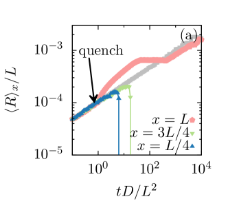
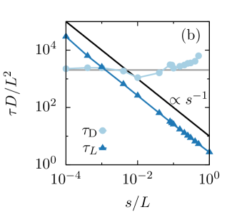
Figure 3: Droplet ripening in concentration gradients. (a) Mean droplet radius $\langle R\rangle_{x}$ at position $x$ as a function of time for different $x$ as indicated. A spatial profile of equilibrium volume fraction of slope $s=0.5$ is imposed at time $t=L^{2}/D$ (quench). The grey data points correspond to classical Ostwald ripening ($s=0$). (b) Characteristic time $\tau_{L}$ required to segregate the volume of droplet material toward $x=L$, and dissolution time $\tau_{\mathrm{D}}$ required to reach $10$ droplets starting from $\mathcal{O}(10^{4})$, as a function of quench slope $s$. The horizontal grey line indicated the value of $\tau_{\mathrm{D}}$ for classical Ostwald ripening ($s=0$).

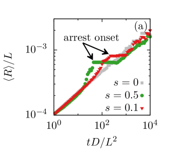
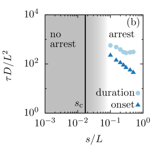
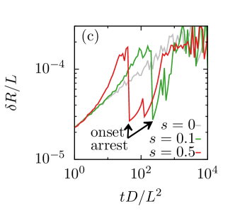
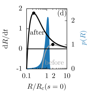
Figure 4: Narrowing droplet size distribution. (a) Mean radius $\langle R\rangle$ averaged over all drops in the system as a function of time for three quench slopes $s$. The onset of arrest is indicated (arrows). (b) Duration and time of onset of the arrest phase as a function of quench slope $s$. The vertical black line indicates the quench slope $s_{\mathrm{c}}=\{1-[3/2-\Phi_{0}/(2\bar{\Phi}(t=L^{2}/D))]^{-1}\}/L$ below which no arrest can occur. It can be calculated by the condition that the critical radius $R_{\mathrm{c}}$ at $x=L$ is reduced by at least a factor of $3/2$ during the quench such that the largest droplets in the distribution grow more slowly than smaller ones and the distribution narrows. For our numerical solutions $s_{\mathrm{c}}\approx 0.017/L$, which is consistent with the emergence of the arrest along quench slope found in our numerical calculations. (c) Standard deviation $\delta R$ of the droplet radius distribution as a function of time for three different quench slopes $s$. The onset of arrest corresponds to a sudden narrowing of the distribution (arrows). (d) Rate of droplet growth $\mathrm{d}R/\mathrm{d}t$ as a function of droplet radius $R$ before (grey) and after (black) the spatial quench. The droplet radius distribution $p(R)$ at the moment of the quench is shown (blue). Narrowing of $p(R)$ occurs if droplet size exceeds the radius for which the growth rate is maximal (black dots).

To study the ripening dynamics of droplets in a concentration gradient we solved the equations (12) to (14) numerically. To access the late time regime of ripening we first initialize about $N=10^{7}$ drops with radii taken from the Lifschitz-Slyozov distribution [9, 10] in a system of position independent equilibrium concentration $\Phi_{0}$, and fix the concetration inside ${\Phi^{\mathrm{in}}_{\mathrm{eq}}}=1$. For $t\geq L^{2}/D$, we then spatially quench the system by imposing the spatially varying equilibrium concentration ${\Phi^{\mathrm{out}}_{\mathrm{eq}}}(x)=\Phi_{0}(1-s\,x)$ [16], which we refer to as “spatial quench” in the following. In our numerical studies we find that droplets experience a non-uniform growth depending on the position and the stage of ripening (figure 3(a)). At the beginning, all drops grow in the region where the concentration $\bar{\Phi}(x)$ exceeds the local equilibrium concentration at the drop surface, ${\Phi^{\mathrm{out}}_{\mathrm{eq}}}(x)\left(1+\ell_{\mathrm{c}}/R\right)$, and shrink otherwise. The dissolution boundary at $x=x_{\mathrm{d}}$ obeys $\bar{\Phi}(x_{\mathrm{d}})\simeq{\Phi^{\mathrm{out}}_{\mathrm{eq}}}(x_{\mathrm{d}})$ since in the late time regime $\ell_{\mathrm{c}}\ll R$. It moves according to

$$\frac{\mathrm{d}x_{\mathrm{d\mathrm{missing}}}}{\mathrm{d}t}={\frac{\mathrm{d}\bar{\Phi}(x_{\mathrm{d}}(t))}{\mathrm{d}t}}\bigg{/}{\left.\frac{\mathrm{d}{\Phi^{\mathrm{out}}_{\mathrm{eq}}}(x)}{\mathrm{d}x}\right|_{x=x_{\mathrm{d}}(t)}}\,.$$ (15)

For $\mathrm{d}{\Phi^{\mathrm{out}}_{\mathrm{eq}}}(x)/\mathrm{d}x<0$, the position of the dissolution boundary $x_{\mathrm{d}}$ moves to the right until it reaches the system boundary at $x=L$ (Supplemental video [17]). At long times, the volume fraction at all positions approaches the minimum of the equilibrium volume fraction, $\bar{\Phi}(x)\to{\Phi^{\mathrm{out}}_{\mathrm{eq}}}(L)$, and all droplets dissolve except at $x=L$ (figure 3(a), Supplemental video [17]).

The characteristic time $\tau_{L}$ of droplet segregation depends on the quench slope $s$. It decreases for increasing $s$ according $\tau_{L}\propto s^{-1}$ (figure 3(b)). In contrast the time of droplet dissolution, $\tau_{\mathrm{D}}$, defined as the time to reach 10 droplets, changes only weakly with the quench slope $s$ and can even increase (figure 3(b)). Interestingly, the droplet ripening exhibits periods of transient arrest, during which droplet number and size remain almost constant (figure 4(a)). These arrest phases govern the time of droplet dissolution for large quench slopes since they occur for sufficiently large quench slopes $s$. The duration of arrest is roughly constant as a function of $s$ and the onset of the arrest phase is delayed for decreasing $s$ [18] (figure 4(b)). Intriguingly, the onset of the arrest phase is preceded by a narrowing of the droplet size distribution. The droplet size distribution narrows during the segregation of droplets toward $x=L$ while the onset of arrest occurs after droplets have mostly been spatially segregated (Supplemental video [17]). In particular, the standard deviation of droplet radius exhibits a pronounced minimum when the arrest begins (figure 4(c)). After the arrest phase droplets undergo classical Ostwald ripening where time-dependence of $\langle R\rangle$ and $\delta R$ is consistent with $t^{1/3}$ (figures 3(a) and 4(a)). The effect of a narrowing droplet size distribution has also been observed in open but spatially homogeneous systems with constant influx of phase separation material [19, 20].

The narrowing of the droplet size distribution in a concentration gradient is fundamentally different from broadening of the droplet size distributions during classical Ostwald-ripening [9, 10]. Ostwald ripening is characterized by a supersaturation that decreases with time, leading to an increase of the critical droplet radius $R_{\mathrm{c}}=\ell_{\mathrm{c}}/\epsilon(t)\propto t^{1/3}$. The droplet size distribution $p(R)$ has a universal shape and is nonzero only in the interval $[0,3R_{\mathrm{c}}/2]$ (figure 4(d), blue graph). The broadening of $p(R)$ follows from larger droplets growing at a larger rate $\mathrm{d}R/\mathrm{d}t$ than smaller droplets. Though $\mathrm{d}R/\mathrm{d}t$ has a maximum at $R=2R_{\mathrm{c}}$ and decreases for large $R$, no droplets exist larger than $3R_{\mathrm{c}}/2$.

This situation changes in the presence of a concentration gradient. The spatial quench reduces the local critical radius $R_{\mathrm{c}}(x\simeq L)=\ell_{\mathrm{c}}/\epsilon(x\simeq L)$ at the rightmost boundary $x\simeq L$ as compared to the critical radius before the quench (equation (5)). This quench also shifts the maximum of $\mathrm{d}R/\mathrm{d}t$ for droplets at $x\simeq L$ to smaller radii (black line in figure 4(d)) since the radius corresponding to the maximum occurs at $R=2R_{\mathrm{c}}$. As a result, many droplets now exist after the spatial quench with large radii $R>2R_{\mathrm{c}}(x\simeq L)$. These droplets grow more slowly than those at $R=2R_{\mathrm{c}}$ which leads to a narrowing of the size distribution $p(R)$ at $x\simeq L$. The critical radius $R_{\mathrm{c}}(x\simeq L)$ remains small because dissolution of droplets at $x<L$ leads to a diffusive flux toward $x\simeq L$ and thus keeps the volume fraction $\bar{\Phi}(L)$ at increased levels. These conditions hold longer if the spatial quench has a steeper slope. As a result the distribution narrows more for steeper quenches. When the critical radius catches up with the mean droplet size narrowing stops and the onset of arrest occurs. At this time droplets have almost equal size which slows down the exchange of material between droplets via Ostwald ripening, leading to a long phase of almost constant size and number of droplets (figure 3(a)). During this arrest phase, the droplet distribution broadens slowly.

6 Conclusion and Outlook

Here we presented the generic behavior of droplet ripening in concentrations gradients and extended the classical theory by Lifschitz & Slyozov to inhomogeneous systems [9, 10]. One main result is that a concentration gradient of a soluble component that regulates liquid-liquid phase separation can reshape the supersaturation profile such that all drops dissolve except those within a region close to one boundary of the system. As a consequence droplets segregate toward the boundary where the supersaturation is highest [7]. Even though the details by which a regulator affects the local supersaturation are system-specific, the resulting ripening dynamics that takes place in a supersaturation gradient is generic. Surprisingly, we find that the size distribution of droplets narrows for sufficiently steep concentration gradients, leading to a transient arrest of the droplet dynamics. Such a behavior is fundamentally different to classical Ostwald-ripening where the droplet size distribution continuously broadens at all times. Transient narrowing of the droplet size distribution stems from a position-dependent shift of the maximal droplet growth rate to smaller droplet radii as compared to spatially homogeneous systems (figure 4(d)).

Our work shows that droplet ripening in concentration gradients exhibits fundamental differences compared to classical phase-separating systems where droplet positions are homogeneously distributed in space. The physics presented here could be relevant for the control of emulsions in chemical engineering and biology. The narrowing of droplet size distributions found in the presence of a regulator gradient could be used to control droplet size in emulsions. It provides a physical mechanism for the formation of almost mono-disperse emulsions. An example in biology where an emulsion is controlled by concentration gradients is the C.elegans embryo [6, 7, 8]. In this system liquid-like cellular compartments, so called P granules, are positioned toward the posterior side of the cell prior to asymmetric cell division by a protein concentration gradient. An increasing number of membrane-less compartments with liquid-like properties have been characterized [2, 21]. Their formation and positioning could be a general scheme for the spatial organization of chemistry in living cells. In our work we have identified the physical mechanisms of spatial segregation of droplets by concentration gradients. The physics discussed here contributes to the behavior of liquid-like compartments in living cells such as P granules. However, many aspects of the dynamics of liquid-like compartments inside cells remain unexplored. In particular, they consist of a large number of components and are chemically active. Emulsions in the presence of chemical reactions driven away from equilibrium can give rise to novel phenomena in phase separating systems such as the suppression of Ostwald ripening [22] or the spontaneous division of liquid droplets [23]. Future questions could address how nucleation, fusion, and droplet shape is changed by concentration gradients and how non-equilibrium chemical reactions in droplets are affected by concentration gradients.

References

References

- [1] Brangwynne CP. Soft active aggregates: mechanics, dynamics and self-assembly of liquid-like intracellular protein bodies. Soft Matter. 2011;7(7):3052–3059.
- [2] Hyman AA, Weber CA, Jülicher F. Liquid-liquid phase separation in biology. Annual review of cell and developmental biology. 2014;30:39–58.
- [3] Brangwynne CP, Tompa P, Pappu RV. Polymer physics of intracellular phase transitions. Nature Physics. 2015;11(11):899–904.
- [4] Cowan CR, Hyman AA. Asymmetric cell division in C. elegans: cortical polarity and spindle positioning. Annu Rev Cell Dev Biol. 2004;20:427–453.
- [5] Betschinger J, Knoblich JA. Dare to be different: asymmetric cell division in Drosophila, C. elegans and vertebrates. Current biology. 2004;14(16):R674–R685.
- [6] Brangwynne CP, Eckmann CR, Courson DS, Rybarska A, Hoege C, Gharakhani J, et al. Germline P Granules Are Liquid Droplets That Localize by Controlled Dissolution/Condensation. Science. 2009;324(5935):1729–1732.
- [7] Lee CF, Brangwynne CP, Gharakhani J, Hyman AA, Jülicher F. Spatial Organization of the Cell Cytoplasm by Position-Dependent Phase Separation. Phys Rev Lett. 2013 Aug;111:088101.
- [8] Saha S, Weber CA, Nousch M, Adame-Arana O, Hoege C, Hein MY, et al. Polar Positioning of Phase-Separated Liquid Compartments in Cells Regulated by an mRNA Competition Mechanism. Cell. 2016;166(6):1572–1584.
- [9] Lifshitz IM, Slyozov VV. The kinetics of precipitation from supersaturated solid solutions. Journal of Physics and Chemistry of Solids. 1961;19(1?2):35 – 50.
- [10] Wagner C. Theorie der Alterung von Niederschlägen durch Umlösen (Ostwald-Reifung). Berichte der Bunsengesellschaft für physikalische Chemie. 1961;65(7):581–591.
- [11] Yao JH, Elder K, Guo H, Grant M. Theory and simulation of Ostwald ripening. Physical review B. 1993;47(21):14110.
- [12] Bray AJ. Theory of phase-ordering kinetics. Advances in Physics. 1994;43(3):357–459.
- [13] Tenlen J, Molk J, London N, Page B, Priess J. MEX-5 asymmetry in one-cell C. elegans embryos requires PAR-4- and PAR-1-dependent phosphorylation. Development. 2008;135(22):3665–3675.
- [14] Griffin E, Odde D, Seydoux G. Regulation of the MEX-5 Gradient by a Spatially Segregated Kinase/Phosphatase Cycle. Cell. 2011;146(6):955–968.
- [15] Rubinstein M, Colby RH. Polymer physics. Oxford: OUP Oxford; 2003.
- [16] We checked that a quench of the form leads to qualitatively similar results;.
- [17] See Supplemental Material for videos and more information at http://;.
- [18] The arrest phase is defined as the time interval during which decreases more slowly then For Ostwald ripening () ;.
- [19] Clark MD, Kumar SK, Owen JS, Chan EM. Focusing Nanocrystal Size Distributions via Production Control. Nano Letters. 2011 may;11(5):1976–1980.
- [20] Vollmer J, Papke A, Rohloff M. Ripening and focusing of aggregate size distributions with overall volume growth. Frontiers in Physics. 2014;2:18.
- [21] Alberti S, Hyman AA. Are aberrant phase transitions a driver of cellular aging? BioEssays. 2016;38(10):959–968.
- [22] Zwicker D, Hyman AA, Jülicher F. Suppression of Ostwald ripening in active emulsions. Phys Rev E. 2015 Jul;92:012317.
- [23] Zwicker D, Seyboldt R, Weber CA, Hyman AA, Jülicher F. Growth and division of active droplets provides a model for protocells. Nature Physics. 2016;10.1038/nphys3984:1745–2481.