A thermodynamically consistent model of magneto-elastic
materials under diffusion at large strains and its analysis.

Abstract.

A theory of elastic magnets is formulated under possible diffusion and heat flow governed by Fick’s and Fourier’s laws in the deformed (Eulerian) configuration, respectively. The concepts of nonlocal nonsimple materials and viscous Cahn-Hilliard equations are used. The formulation of the problem uses Lagrangian (reference) configuration while the transport processes are pulled back. Except the static problem, the demagnetizing energy is ignored and only local non-selfpenetration is considered. The analysis as far as existence of weak solutions of the (thermo)dynamical problem is performed by a careful regularization and approximation by a Galerkin method, suggesting also a numerical strategy. Either ignoring or combining particular aspects, the model has numerous applications as ferro-to-paramagnetic transformation in elastic ferromagnets, diffusion of solvents in polymers possibly accompanied by magnetic effects (magnetic gels), or metal-hydride phase transformation in some intermetalics under diffusion of hydrogen accompanied possibly by magnetic effects (and in particular ferro-to-antiferromagnetic phase transformation), all in the full thermodynamical context under large strains.

1 Introduction

Recent experiments have been putting into perspective interesting interplay between hydrogenation and magnetic properties of ferromagnetic specimens. At the microscopic level, the atomic lattice parameters are substantially enlarged when diffusing hydrogen atoms occupy the interstitial positions without changing the cubic (or sometimes hexagonal) structure, leading to large strains. We the speak about metal-to-hydride phase transformation. If the metal is ferromagnetic, the resulted hydride may be antiferromagnetic, as documented experimentally e.g. in [42, 51]. Of course, this phase transformation is in addition to the ferro-to-paramagnetic phase transformation in the parent metal phase when temperature rises the Curie point. Also specific heat can be substantially influenced by the concentration of hydrogen, as experimentally documented in the case of the hydrogenization/deuterization of some intermetalics e.g. in [51]. Although mathematical models of hydrogenation have been formulated and studied specifically for hydrogen storage with [15, 48] or without [5, 6] strain effects these models do not take into account large strains and the interaction between diffusant and magnetization, see also [27, 28, 29, 30, 31].

Besides specific applications to hydrogenation, our model can cover situations when magnetic effects are coupled with substantial large strains, such as elastomers [7] and polymer gels [12, 4] with magnetic inclusions. These materials are obtained by embedding metallic or ferromagnetic particles into solid matrix and can undergo controlled large strains, with potential applications for biomechanics and biomimetics [57].

We also point out that instead of magnetization, one can thus equally think about polarization and ferroelectric materials instead of ferromagnetic.

The range of applicability of the model is the ability of magnetic-field-sensitive gels to undergo a quick controllable change of shape can be used to create an artificially designed system possessing sensor- and actuator functions internally in the gel itself. The peculiar magneto-elastic properties may be used to create a wide range of motion and to control the shape change and movement, that are smooth and gentle similar to that observed in muscle. Magnetic field sensitive gels provide attractive means of actuation as artificial muscle for biomechanics and biomimetic applications.

To partially fill this gap, in this paper we propose and study a large-strain thermomechanical model describing a magnetized solid permeated by a diffusant and undergoing non-isothermal processes. As usual for solid mechanics, we formulate the problem in the referential setting, choosing as reference configuration an unbounded domain ${\varOmega}\subset\mathbb{R}^{d}$ having a Lipschitz boundary ${\varGamma}=\partial{\varOmega}$. At variance with most treatments in ferromagnetism [8] we do not impose the saturation (so called Heisenberg) constraint on the magnitude of the magnetization which is, in fact, relevant rather only below the Curie point, cf. also the discussion in [41] and references cited therein.

Rather as a side effect, forgetting magnetic long-range interaction, the model covers also the flow in poro-elastic materials at large strains, as e.g. rocks or soils.

Our ultimate goal is to develop a model which is both thermodynamically consistent and also amenable to mathematical analysis. Let us briefly summarize the mathematical challenges set forth by the problem we examine:

While existence of minimizers in nonlinear elastostatics is well understood, the question whether these minimizers correspond to actual weak solutions of the Euler-Lagrange equations is an open issue [2], essentially because the strain energy blows up as the determinant of the deformation gradient tends to null. Such technical hindrance is exacerbated when, instead of looking for weak solutions in nonlinear elastostatics, one considers the evolution problem of nonlinear elastodynamics.

In addition, handling the effects of magnetization and diffusion at large strains requires some care. In fact, the equations of magnetostatics are naturally formulated in the actual configuration and, in order to pull the relevant fields back to the reference configuration the injectivity of the deformation map is mandatory. Now, while the injectivity of the deformation map can be guaranteed in the variational setting by enforcing the Ciarlet-Nečas condition [11], this is not mathematically feasible when seeking weak solutions of the evolution equations of nonlinear elastodynamics.

Second, the Fick-type relations between the flux of the diffusant and its driving force, namely, the gradient of chemical potential, as well as the Fourier law relating heat flux and temperature gradient, are often formulated in the deformed configuration (see for example [14]). When these constitutive laws are pulled back to the reference configuration (see (3.16) below), the reciprocal of the determinant of the deformation gradient enters into play, it would be desirable to have the determinant is away from zero.

Following an idea from [23], we will include in the free energy a regularizing term to ensure that the determinant of the deformation gradient stays away from zero, cf. also Lemma 1 below. However, since we are interested in performing mathematical analysis also in the dynamical setting, we opt for a quadratic regularizing term, whose contribution to the Fréchet derivative of the free energy has the nice property of being linear, which makes it possible to pass to the limit in the nonlinear hyperbolic problem in our proof of existence of weak solutions, see Sec. 4 below. Now, it turns out that in order for this approach to work, the deformation gradient should be at least in the Sobolev-Slobodetskiĭ space $H^{2+\gamma}$, with $\gamma$ a positive exponent smaller than 1. To meet this requirement, one option would be to consider a local non-simple material of grade 3, whose free energy depends on the third gradient of the deformation. Instead, we have chosen a model consistent with the definition of the space $H^{2+\gamma}$, namely, the space of functions in $H^{2}$ whose second gradient is in the fractional space $H^{\gamma}$.

The model which we adopt thus involves a nonlocal dependence on the second gradient, combining therefore the concept of gradient-theories for strains, which is usually referred as nonsimple, cf. [55] or also e.g. [21, 38, 40, 52, 56], with the nonlocal concept like that introduced, for instance, in [18] with the nonlocality in the first gradients, however. Thus, this model may be referred to as material of grade $2+\gamma$ or also be regarded as a 2nd-grade non-simple material cf. Remark 2.

The other higher-order contribution to the free energy involving $\nabla\bm{m}$ and $\nabla\zeta$ are quite standard and widely accepted. In particular, as in standard micromagnetics, $\nabla\bm{m}$ models exchange interactions by including a gradient term on the magnetization [8]. As far as concentration of diffusant is concerned, $\nabla\zeta$ includes an interfacial energy of Cahn-Hilliard type [9]. This leads us to the overall thermomechanical Helmholtz free energy formulated in the reference configuration:

$$\mathcal{H}_{\rm th}(\bm{\chi},\bm{m},\zeta,\theta)=\int_{\varOmega}\psi(\nabla\bm{\chi},\bm{m},\zeta,\theta)+\frac{\kappa_{1}}{2}|\nabla\bm{m}|^{2}+\frac{\kappa_{2}}{2}|\nabla\zeta|^{2}\,\mathrm{d}x+\mathscr{H}(\nabla^{2}\bm{\chi}),$$ (1.1)

where, using the placeholder ${\mathbb{G}}$ for $\nabla^{2}\bm{\chi}$, we define the quadratic form

$$\mathscr{H}({\mathbb{G}}):=\frac{1}{4}\int_{\varOmega}\int_{\varOmega}({\mathbb{G}}(x){-}{\mathbb{G}}(\tilde{x}))^{\top}\vdots\mathscr{K}(x{-}\tilde{x})\vdots({\mathbb{G}}(x){-}{\mathbb{G}}(\tilde{x}))\,\mathrm{d}x\mathrm{d}\tilde{x}\color[rgb]{0,0,0},\color[rgb]{0,0,0}$$ (1.2)

where the kernel $\mathscr{K}:\mathbb{R}^{d}\to{\mathbb{R}^{d}}^{6}$ takes values in the space of sixth-order tensors. Here we adopt the convention triple dots joining a sixth-order tensor (here $\mathscr{K}$) and a third-order tensor (here ${\mathbb{G}}(x){-}{\mathbb{G}}(\tilde{x})$) denote contraction of the last three indices of the former with the indices of the latter. More generally, we denote by “$\,\cdot\,$” and “$\,:\,$” and “$\,\vdots\,$”, the scalar product between vectors, tensors, and 3rd-order tensors, respectively. For our mathematical purpose, it will be desired if the kernel is singular around the origin, having the asymptotic character

$$\exists\,\epsilon>0\ \forall\,x\!\in\!\mathbb{R}^{d},\ |x|\leq\epsilon:\ \ \ \color[rgb]{0,0,0}\inf_{|{\mathbb{G}}|=1}{\mathbb{G}}^{\top}\vdots\mathscr{K}(x)\vdots{\mathbb{G}}\geq\epsilon\color[rgb]{0,0,0}/|x|^{d+2\gamma}.$$ (1.3)

As pointed out above, the growth condition (1.3) is inspired by the usual Gagliardo seminorm on Sobolev-Slobodetskiĭ space $H^{2+\gamma}({\varOmega};\mathbb{R}^{d})$. Cf. also Remark 2 below for a discussion of the mechanical concept.

The state variables are the displacement $\bm{\chi}$, the magnetization $\bm{m}$, concentration $\zeta$ of a diffusant (typically some liquid, gas, or some solvent and, depending on specific applications, it may be hydrogen, deuterium, water, etc.), and (absolute) temperature $\theta$. The particular equations of the system considered in this paper are the momentum equilibrium, the flow rule for magnetization, the balance of mass of the diffusant, and the heat-transfer equation. The basic notation is summarized in Table 1.

$\varOmega$ the reference domain
$\bm{\chi}$ deformation
$\Omega=\bm{\chi}(\varOmega)$ the actual deformed domain
$\varGamma$ the boundary of $\varOmega$
$\bm{v}$ velocity
$\bm{m},\bm{\mathsf{m}}$ magnetization vectors
$\zeta$ concentration
$\theta$ temperature
$\bm{F}$ deformation gradient
$\bm{C}$ right Cauchy-Green tensor
${\mathbb{G}}$ gradient of $\bm{F}$
$\bm{S}$ stress tensor
$\mathfrak{H}$ hyperstress 3rd-order tensor
$\mathscr{H}$ potential of the hyperstress
$\mu$ chemical potential
$\phi,\upphi$ magnetic potentials
$\bm{M},\bm{\mathsf{M}}$ mobility tensors
$\bm{K},\bm{\mathsf{K}}$ heat-conductivity tensors $\varrho$ mass density
$\psi$ free energy
$s$ entropy
$e_{\textsc{th}}=w$ thermal part of internal energy
$c_{\rm v}=c_{\rm v}(\bm{m},\zeta,\theta)$ heat capacity
$\upmu_{0}$ vacuum permeability
$\psi_{\textsc{me}},\psi_{\textsc{th}}$ chemo-mechanical and thermal free energies
$\bm{f},\bm{\mathsf{f}}$ bulk forces (e.g. gravity)
$\bm{g}$ traction force
$\bm{h}_{\rm e},\bm{\mathsf{h}}_{\rm e}$ external magnetic field
$\mu_{\rm e}$ boundary chemical potential
$K>0$ transmission coefficient for heat supply on $\varGamma$
$M>0$ transmission coefficient for diffusant on $\varGamma$
$\varepsilon>0$ a regularization parameter
$k\in\mathbb{N}$ a numbering of the Galerkin space discretisation
$r$ heat-production rate
$\tau_{1},\tau_{2}>0$ relaxation times
$\kappa_{1},\kappa_{2}>0$ length-scale parameters

Table 1.  Summary of the basic notation used through this paper. The Italics font indicates the reference material (Lagrangian) configuration (as in Fig. 1) while Roman indicated the actual deformed (Eulerian) configuration.

The plan of the paper is the following. In Section 2 we explore equilibrium states, that is rest states characterized by uniform temperature and chemical potential. This will allow us to carry out the rigorous mathematical treatment of a model that takes into account the complete energetic of the system. In particular, we shall be able to handle the demagnetizing energy by guaranteeing the invertibility of the deformation through the Ciarlet-Nečas [11] condition

$$\int_{\varOmega}\det(\nabla\bm{\chi}(x))\,\mathrm{d}x\leq{\rm meas}_{d}(\bm{\chi}({\varOmega}))$$

which, together with $\det(\nabla\bm{\chi})>0$ a.e. on ${\varOmega}$, ensures existence of $\bm{\chi}^{-1}$ a.e. on $\bm{\chi}({\varOmega})$. In Section 3 we lay down the evolution system, including all relevant thermodynamical couplings. We show existence of weak solutions in Section 4. This is, to some extent, a constructive method which suggest (when using e.g. finite-element method for the Galerkin approximation) a numerically stable and convergent computationally implementable strategy for solution of the dynamical problem.

Thorough the whole paper, we will use the standard notation for the Lebesgue $L^{p}$-spaces and $W^{k,p}$ for Sobolev spaces whose $k$-th distributional derivatives are in $L^{p}$-spaces. We will also use the abbreviation $H^{k}=W^{k,2}$. Moreover, we use the standard notation $p^{\prime}=p/(p{-}1)$, and $p^{*}$ for the Sobolev exponent $p^{*}=pd/(d{-}p)$ for $p<d$ while $p^{*}<\infty$ for $p=d$ and $p^{*}=\infty$ for $p>d$, and the “trace exponent” $p^{\sharp}$ defined as $p^{\sharp}=(pd{-}p)/(d{-}p)$ for $p<d$ while $p^{\sharp}<\infty$ for $p=d$ and $p^{\sharp}=\infty$ for $p>d$. Thus, e.g., $W^{1,p}({\varOmega})\subset L^{p^{*}}\!({\varOmega})$ or $L^{{p^{*}}^{\prime}}\!({\varOmega})\subset W^{1,p}({\varOmega})^{*}$= the dual to $W^{1,p}({\varOmega})$. In the vectorial case, we will write $L^{p}({\varOmega};\mathbb{R}^{n})\cong L^{p}({\varOmega})^{n}$ and $W^{1,p}({\varOmega};\mathbb{R}^{n})\cong W^{1,p}({\varOmega})^{n}$. Also, we admit $k$ noninteger with the reference to the Sobolev-Slobodetskiĭ spaces. Note that, in this notation, we have the compact embedding $H^{2+\gamma}({\varOmega})\subset W^{2,p}({\varOmega})$ if $p>2d/(d-2\gamma)$ and $W^{2,p}({\varOmega})\subset W^{1,p^{*}}({\varOmega})$. In particular $H^{2+\gamma}({\varOmega})\subset C^{1}(\bar{\varOmega})$ if $d<p<2d/(d-2\gamma)$, which can be satisfied if $\gamma>d/2-1$ as employed in (2.21b) to facilitate usage of the results from [23]. We also denote by $\operatorname{meas}_{d}$ the $d$-dimensional Hausdorff measure.

2 Static model in the Lagrangian formulation

Null entropy production is an essential character of equilibrium states, a character that distinguishes them from the more encompassing class of rest (i.e. steady) states. In the presence of thermal conduction and chemical diffusion, null entropy production demands that the heat flux and the flux of diffusant vanish (for a general discussion in the context of classical continuum thermodynamics we refer to [53, Chap. 13]).

In this section we investigate the existence of equilibrium states for a body in a conservative mechanical environment and thermal and chemical environment of isolation type. The first part of this section is dedicated to the construction of the internal energy and the potential energy. As usual, for the purpose of the derivation of the model, we shall assume that all fields of interest are as smooth as needed for our manipulations to make sense.

State variables.

We identify a rest state with the following quadruplet of state fields:

• the deformation $\bm{\chi}:\varOmega\to\mathbb{R}^{d}$;

• the Lagrangian magnetization $\bm{m}:\varOmega\to\mathbb{R}^{d}$;

• the concentration $\zeta:\varOmega\to\mathbb{R}^{+}$;

• the temperature $\theta:\varOmega\to\mathbb{R}^{+}$.

These fields are defined on the reference configuration $\varOmega$, which we assume to be an open, bounded smooth domain in $\mathbb{R}^{d}$, with $d$ the space dimension.

In this section, we shall work with admissible deformations that are one-to-one, locally orientation-preserving mappings. Local orientation preservation is the requirement that the determinant of the deformation gradient be positive:

$$J=\operatorname{det}\bm{F}>0,\qquad\bm{F}=\nabla\bm{\chi}.$$ (2.1)

If this requirement is met, global invertibility can be guaranteed through the condition

$$\int_{\varOmega}J\,\mathrm{d}x\leq{\rm meas}_{d}(\bm{\chi}({\varOmega})),$$ (2.2)

which was introduced by Ciarlet & Nečas [11] as a device to preclude minimizers of the variational problem of nonlinear elastostatic from self-penetration, and later used in the context of static magneto-elasticity in [43, 44].

These requirements on the deformation are essential to attribute physical meaning to the referential fields $\bm{m}$, $\zeta$, and $\theta$. Indeed, from the knowledge of these fields one can reconstruct the spatial magnetization density in the body, the spatial concentration in the body, and the spatial temperature in the body, respectively,

$$\bm{\mathsf{m}}:\Omega\to\mathbb{R}^{d},\qquad\upzeta:\Omega\to\mathbb{R}^{+},\qquad\text{and}\qquad\uptheta:\Omega\to\mathbb{R}^{+},$$ (2.3)

where

$$\Omega=\bm{\chi}(\varOmega)$$ (2.4)

is the region occupied by the body in its actual configuration. These fields are defined by

$$\bm{\mathsf{m}}=(J^{-1}\bm{F}\bm{m}){\circ}\bm{\chi^{-1}},\qquad\upzeta=(J^{-1}\zeta){\circ}\bm{\chi}^{-1},\qquad\text{and}\qquad\uptheta=\theta{\circ}\bm{\chi}^{-1}.$$ (2.5)

The spatial fields are more amenable to physical interpretation than the corresponding referential quantities, since their value at a point $z\in\Omega$ represents quantities that in principle are accessible to physical measurement. Precisely: $\bm{\mathsf{m}}(z)$ is the density of magnetic moments per unit spatial volume; $\upzeta(z)$ is the density of diffusant per unit spatial volume; $\uptheta(z)$ is the temperature in the position $z$.

The environment.

As we have anticipated, we assume that the chemical environment is of isolation type. This means that the flux of chemical species vanish at the boundary. On account of this we impose, as a constraint, the total amount of chemical species be equal to a given constant:

$$\int_{\varOmega}\zeta\,\mathop{{\rm d}x}=Z_{\rm tot}.$$

We next specify the standard mechanical interaction of the body with its environment. To this effect, we assume that the body is clamped on a part $\varGamma_{\rm D}$ of $\partial\Omega$ having positive Hausdorff two-dimensional measure. Accordingly, we require that admissible deformations satisfy

$$\bm{\chi}=\bm{\chi}_{\rm D}\ \text{ on }\ \varGamma_{\rm D},$$ (2.6)

with $\bm{\chi}_{\rm D}$ given. We model interaction with the environment of purely mechanical origin through the mechanical potential energy [10]:

$$\mathcal{L}(\bm{\chi}):=\int_{\varOmega}\bm{f}\cdot\bm{\chi}\mathop{{\rm d}x}+\int_{{\varGamma}_{\rm N}}\bm{g}\cdot\bm{\chi}\operatorname{d}\!S,$$ (2.7)

where $\bm{g}:\varGamma_{\rm N}\to\mathbb{R}^{d}$ and $\bm{f}:\Omega\to\mathbb{R}^{3}$ is a system of dead loads, see Fig. 1. Let us remark that, in fact, more general load is possible in particular also on the boundary due to the used concept of nonsimple materials, but we do not want to bring additional technicalities into the model.

We next turn to the description of magnetic interactions with the environment. Such interactions depend on magnetic moments associated to possibly electric currents or other magnetized bodies outside the region $\Omega$. We take these interaction collectively into account through the following magnetic potential energy:

$$\mathcal{Z}(\bm{\chi},\bm{m})\color[rgb]{0,0,0}=\int_{{\varOmega}}\!\bm{h}_{\rm e}\cdot{\bm{m}}\,\mathrm{d}x$$ (2.8)

where $\bm{h}_{\rm e}:\varOmega\to\mathbb{R}^{d}$, the Lagrangian external magnetic field, depends on $\bm{\chi}$ through the relation

$$\bm{h}_{\rm e}=\bm{F}^{\top}[\bm{\mathsf{h}}_{\rm e}{\circ}\bm{\chi}],\qquad\bm{F}=\nabla\bm{\chi},$$ (2.9)

with $\bm{\mathsf{h}}_{\rm e}:\mathbb{R}^{d}\to\mathbb{R}^{d}$ an externally imposed magnetic field. From the first of (2.5), we have

$$\bm{m}=J\,\bm{F}^{-1}\,[\bm{\mathsf{m}}{\circ}\bm{\chi}],$$ (2.10)

and hence

$$\mathcal{Z}(\bm{\chi},\bm{m}) =\int_{\varOmega}\!\Big{(}\bm{F}^{\top}[\bm{\mathsf{h}}_{\rm e}{\circ}\bm{\chi}]\Big{)}\cdot\Big{(}J\color[rgb]{0,0,0}\bm{F}^{-1}[\bm{\mathsf{m}}{\circ}\bm{\chi}]\Big{)}\,\mathrm{d}x$$

$$=\int_{\varOmega}\![\bm{\mathsf{h}}_{\rm e}{\circ}\bm{\chi}]\cdot[\bm{\mathsf{m}}{\circ}\bm{\chi}]J\,\mathrm{d}x=\int_{\bm{\chi}({\varOmega})}\bm{\mathsf{h}}_{\rm e}\cdot\bm{\mathsf{m}}\,\mathrm{d}z=\int_{\mathbb{R}^{d}}\!\bm{\mathsf{h}}_{\rm e}\cdot\overline{\bm{\mathsf{m}}}\,\mathrm{d}z.$$ (2.11)

where, for $\bm{\mathsf{m}}$ defined in (2.5),

$$\overline{\bm{\mathsf{m}}}:\mathbb{R}^{d}\to\mathbb{R}^{d},\qquad\text{defined by }\overline{\bm{\mathsf{m}}}(z)=\left\{\begin{array}[]{ll}\bm{\mathsf{m}}(z)&\text{if }z\in\Omega,\\[3.99994pt] \bm{0}&\text{otherwise},\end{array}\right.$$ (2.12)

is the trivial extension of $\bm{\mathsf{m}}$ to $\mathbb{R}^{d}$. It is easy to check that the last term in the chain of equalities (2.11) coincides with the standard Zeeman energy [24].

An illustration of the relation between the spatial and Lagrangian fields of interest is in Fig. 1.

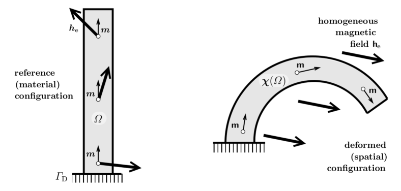
Figure 1: Sketch of the relation between the Lagrangian magnetization $\bm{m}=J\bm{F}^{-1}[\bm{m}{\circ}\bm{\chi}^{-1}]$ and external magnetic field $\bm{h}_{\rm e}=\bm{F}^{\top}[\bm{\mathsf{h}}_{\rm e}{\circ}\bm{\chi}^{-1}]$ and their spatial counterparts $\bm{\mathsf{m}}$ and $\bm{\mathsf{h}}_{\rm e}$. In the present case we consider a body that is elastically soft and magnetically hard with homogeneous Lagrangian magnetization $\bm{m}$. The body is fixed at the bottom by Dirichlet condition is deformed in a spatially-constant external magnetic field $\bm{\mathsf{h}}_{\rm e}$.

The free energy of the body.

The total Helmholtz free energy is the sum

$$\mathcal{H}(\bm{\chi},\bm{m},\zeta,\theta)=\mathcal{H}_{\rm th}(\bm{\chi},\bm{m},\zeta,\theta)+\mathcal{H}_{\rm mag}(\bm{\chi},\bm{m})$$ (2.13)

of the thermomechanical free energy $\mathcal{H}_{\rm th}(\bm{\chi},\bm{m},\zeta,\theta)$ defined in (1.1) and the magnetostatic free energy [24]:

$$\mathcal{H}_{\rm mag}(\bm{\chi},\bm{m})=\frac{\upmu_{0}}{2}\int_{\mathbb{R}^{d}}|\operatorname{\mathsf{grad}}\upphi|^{2}\,\mathrm{d}z,$$ (2.14)

where $\upmu_{0}$ is the permeability of vacuum and where $\upphi$, the spatial scalar magnetic potential, is a solution of

$$-\operatorname{\sf{div}}\big{(}\mu_{0}\operatorname{\mathsf{grad}}\upphi\big{)}=\operatorname{\sf{div}}\big{(}\overline{\bm{\mathsf{m}}}\big{)}\quad\text{on }\ \mathbb{R}^{d}\ \text{ with }\ \overline{\bm{\mathsf{m}}}\text{ from }\eqref{m-pull-back}\text{ and }\eqref{eq:12}$$ (2.15)

in the sense of distributions; to be more specific, we also consider a “boundary condition at $\infty$” by seeking a solution to (2.12) in $H^{1}(\mathbb{R}^{d})$, cf. Theorem 1 below.

On using $\upphi_{\bm{\chi},\bm{m}}$ as a test function in (2.15) we find

$$\mathcal{H}_{\rm mag}(\bm{\chi},\bm{m}) {}={}\frac{1}{2}\int_{\mathbb{R}^{d}}\!\!{\mathsf{grad}}\upphi\cdot\overline{\bm{\mathsf{m}}}\,\mathrm{d}z{}={}\frac{1}{2}\int_{\bm{\chi}({\varOmega})}\!\!{\mathsf{grad}}\upphi\cdot\bm{\mathsf{m}}\,\mathrm{d}z.$$

Moreover, by introducing the referential scalar magnetic potential

$$\phi=\upphi{\circ}\bm{\chi},$$ (2.16)

we have

$$\operatorname{\mathsf{grad}}\upphi=[\bm{F}^{-\!\top}\nabla\phi]{\circ}\bm{\chi}^{-1}\qquad\text{in }\Omega,$$ (2.17)

hence, on recalling (2.10), we can write, by changing from $\bm{\chi}(\varOmega)$ to $\varOmega$ the domain of integration,

$$\mathcal{H}_{\rm mag}(\bm{\chi},\bm{m}) ={}\frac{1}{2}\int_{\varOmega}\!\big{(}\bm{F}^{-\!\top}\nabla\phi\big{)}\cdot[\bm{\mathsf{m}}{\circ}\bm{\chi}]J\,\mathrm{d}x=\frac{1}{2}\int_{\varOmega}\!\nabla\phi\cdot J\bm{F}^{-1}[\bm{\mathsf{m}}{\circ}\bm{\chi}]\,\mathrm{d}x=\frac{1}{2}\int_{{\varOmega}}\!\nabla\phi{\cdot}{\bm{m}}\,\mathrm{d}x.$$ (2.18)

By combining (1.1), (2.13), and (2.18), we obtain the total Helmholtz free energy of the body:

$$\mathcal{H}(\bm{\chi},\bm{m},\zeta,\theta)=\int_{\Omega}\psi(\nabla\bm{\chi},\bm{m},\zeta,\theta)+\frac{\kappa_{1}}{2}|\nabla\bm{m}|^{2}+\frac{\kappa_{2}}{2}|\nabla\zeta|^{2}+\frac{1}{2}\mathfrak{H}(\nabla^{2}\bm{\chi})\vdots\nabla^{2}\bm{\chi}+\frac{1}{2}\nabla\phi\cdot\bm{m}\,\mathrm{d}x,$$ (2.19)

Here $\mathfrak{H}:=\mathscr{H}^{\prime}$ is the (Gâteaux) derivative of the nonlocal energy $\mathscr{H}$ defined in (1.2), namely

$$[\mathfrak{H}({\mathbb{G}})](x):=\big{[}\mathscr{H}^{\prime}({\mathbb{G}})\big{]}(x)=\int_{\varOmega}\mathscr{K}(x{-}\tilde{x})\vdots({\mathbb{G}}(x){-}{\mathbb{G}}(\tilde{x}))\,\mathrm{d}\tilde{x},$$ (2.20)

as can be seen by the Fubini theorem to evaluate the nonlocal hyperstress explicitly provided the symmetry of $\mathscr{K}$ in the sense $\mathscr{K}(x)=\mathscr{K}(-x)$ is additionally assumed.

Assumptions on the bulk free energy.

We assume that the bulk free-energy mapping $\psi$ is continuous and twice-continuously differential with respect to $\theta$ on $[0,+\infty)$. We also assume that it satisfies the frame indifference and exhibits a (sufficiently fast) blow-up when ${\rm det}\bm{F}$ approaches zero in order to prevent local self-penetration, and that it is a strictly concave function and coercive at infinity with respect to $\theta$. Thus, we require

$$\forall\bm{Q}\in{\rm SO}(d):\quad\ \psi(\bm{Q}\bm{F},\bm{m},\zeta,\theta)=\psi(\bm{F},\bm{m},\zeta,\theta),$$ (2.21a)

$${\rm det}\bm{F}>0\ \ \ \Rightarrow\ \ \ \psi(\bm{F},\bm{m},\zeta,\theta)\geq\epsilon/({\rm det}\bm{F})^{p}\ \ \text{ for some}\ \ p>\frac{2d}{\color[rgb]{0,0,0}2\gamma{+}2{-}d\color[rgb]{0,0,0}},\ \ \gamma>d/2{-}1,$$ (2.21b)

$${\rm det}\bm{F}\leq 0\ \ \ \Rightarrow\ \ \ \psi(\bm{F},\bm{m},\zeta,\theta)=\infty$$ (2.21c)

$$\forall{\bm{Q}}\!\in\!\mathrm{SO}(d)\ \forall{\mathbb{G}}\!\in\!\mathbb{R}^{d\times d\times d}:\!\sum_{i,j,k,l,m,n=1}^{d}\!\!\!\!\!\!{Q}_{in}G_{njp}\mathscr{K}_{ijpklq}(x){Q}_{km}G_{mlq}=\sum_{i,j,k,l,m,n=1}^{d}\!\!\!\!\!\!G_{ijp}\mathscr{K}_{ijpklq}(x)G_{klq},$$ (2.21d)

$$-\partial^{2}_{\theta\theta}\psi(\bm{F},\bm{m},\zeta,\theta)>0,\ \ \lim_{\theta\to 0+}\partial_{\theta}\psi(\bm{F},\bm{m},\zeta,\theta)\leq C,\ \text{ and }\ \lim_{\theta\to+\infty}\partial_{\theta}\psi(\bm{F},\bm{m},\zeta,\theta)=-\infty,$$ (2.21e)

$$\lim_{\theta\to+\infty}\frac{\psi(\bm{F},\bm{m},\zeta,\theta)}{\theta^{\delta}}=0\ \text{ for some}\ \delta>1,$$ (2.21f)

$$\psi(\bm{F},\bm{m},\zeta,s)\leq C\left(1+|\bm{m}|^{\color[rgb]{0,0,0}q\color[rgb]{0,0,0}}+|\zeta|^{\color[rgb]{0,0,0}q\color[rgb]{0,0,0}}\right)\color[rgb]{0,0,0}\ \ \ \text{ with some }\ 1\leq q<2d/(d{-}2)\color[rgb]{0,0,0}\color[rgb]{0,0,0}.$$ (2.21g)

for some $\epsilon>0$, $C\color[rgb]{0,0,0}<+\infty\color[rgb]{0,0,0}$, and with $\gamma$ the exponent appearing in (1.3). Here $Q_{ij}$, $G_{mlq}$, $\mathscr{K}_{ijpklq}$ denote the Cartesian components of the tensors $\bm{Q}$, ${\mathbb{G}}$, and $\mathscr{K}$ respectively; moreover ${\rm SO}(d):=\{\bm{Q}\in\mathbb{R}^{d\times d};\ \bm{Q}^{\top}=\bm{Q}^{-1},\ \det\bm{Q}>0\}$ denoting the special orthogonal group (i.e. the group of orientation-preserving rotations). The nonlocal energy $\mathscr{H}$ defined in (1.2) enjoys frame-indifference in the sense that $\mathscr{H}({\mathbb{G}})=\mathscr{H}({\bm{Q}}{\mathbb{G}})$ for all ${\bm{Q}}\in\mathrm{SO}(d)$ for any field ${\mathbb{G}}:{\varOmega}\to\mathbb{R}^{d\times d\times d}$ (here $({\bm{Q}}{\mathbb{G}})_{ijk}=Q_{il}G_{ljk}$).

Entropy as state variable.

The total free energy is defined as the total Helmholtz free energy minus the potential energy of the environment,

$$\mathcal{P}(\bm{\chi},\bm{m},\zeta,\theta)=\mathcal{H}(\bm{\chi},\bm{m},\zeta,\theta)-\mathcal{L}(\bm{\chi})-\mathcal{Z}(\bm{\chi},\bm{m}),$$

where we recall that $\mathcal{H}$, $\mathcal{L}$, and $\mathcal{Z}$ are defined in (2.19), (2.7), and (2.8), respectively. Accordingly, the total energy is

$$\mathcal{U}(\bm{\chi},\bm{m},\zeta,\theta)=\mathcal{E}(\bm{\chi},\bm{m},\zeta,\theta)-\mathcal{L}(\bm{\chi})-\mathcal{Z}(\bm{\chi},\bm{m}),$$

where

$$\mathcal{E}(\bm{\chi},\bm{m},\zeta,\theta)=\int_{\Omega}e(\nabla\bm{\chi},\bm{m},\zeta,\theta)+\frac{\kappa_{1}}{2}|\nabla\bm{m}|^{2}+\frac{\kappa_{2}}{2}|\nabla\zeta|^{2}+\frac{1}{2}\mathfrak{H}(\nabla^{2}\bm{\chi})\vdots\nabla^{2}\bm{\chi}+\frac{1}{2}\nabla\phi\cdot\bm{m}\,\mathrm{d}x,$$

with

$$e(\bm{F},\bm{m},\zeta,\theta)=\psi(\bm{F},\bm{m},\zeta,\theta)+\theta s(\bm{F},\bm{m},\zeta,\theta),\qquad s(\bm{F},\bm{m},\zeta,\theta)=-\partial_{\theta}\psi(\bm{F},\bm{m},\zeta,\theta)$$ (2.22)

being, respectively, the bulk internal energy and the entropy.

The Principle of Minimum of the Total Energy [53, 15.2.4] states that stable equilibrium states minimize the total energy $\mathcal{U}$ under the constraint that the total entropy be constant:

$$\int_{\varOmega}s(\bm{F},\bm{m},\zeta,\theta)\,\mathop{{\rm d}x}=S_{\rm tot}.$$ (2.23)

When using this principle as selection criterion, we find it convenient to replace temperature with entropy as independent field, a device that makes it easier for us to handle the constraint (2.23). Such device is at our disposal thanks to Assumption (2.21e), which entails that the mapping

$$\mathbb{R}^{+}\ni\theta\mapsto s(\bm{\chi},\bm{m},\zeta,\theta)\in[s_{\rm min}(\bm{F},\bm{m},\zeta),+\infty)$$

is strictly concave for every choice of the arguments $(\bm{F},\bm{m},\zeta)$, hence it is invertible, with the lower bound on entropy $s_{\rm min}(\bm{F},\bm{m},\zeta)=s(\bm{F},\bm{m},\zeta,0)\geq-C$ being a consequence of (2.21e). To this effect, Convex Analysis comes in hand, for one can check that the mapping that delivers the bulk internal energy $e$ as function of the state variables $(\bm{F},\bm{m},\zeta,s)$ is the Legendre transform of $-\psi$. We set

$$\widetilde{e}(\nabla\bm{\chi},\bm{m},\zeta,s)=\sup_{\theta\in\color[rgb]{0,0,0}\mathbb{R}\color[rgb]{0,0,0}}\psi_{*}(\nabla\bm{\chi},\bm{m},\zeta,\theta)+\theta s,$$ (2.24a)

where $$\psi_{*}(\nabla\bm{\chi},\bm{m},\zeta,\cdot) \psi(\nabla\bm{\chi},\bm{m},\zeta,\cdot) \mathbb{R}$$ is the unique continuously differentiable affine extension of to .

As desired, we now have the expression of the internal energy

$$\widetilde{\mathcal{E}}(\bm{\chi},\bm{m},\zeta,s)=\int_{\Omega}\widetilde{e}(\nabla\bm{\chi},\bm{m},\zeta,s)+\frac{\kappa_{1}}{2}|\nabla\bm{m}|^{2}+\frac{\kappa_{2}}{2}|\nabla\zeta|^{2}+\frac{1}{2}\mathfrak{H}(\nabla^{2}\bm{\chi})\vdots\nabla^{2}\bm{\chi}+\frac{1}{2}\nabla\phi\cdot\bm{m}\,\mathrm{d}x,$$ (2.24b)

as function of entropy at our disposal. We can then define the total energy as:

$$\widetilde{\mathcal{U}}(\bm{\chi},\bm{m},\zeta,s)=\begin{cases}&\widetilde{\mathcal{E}}(\bm{\chi},\bm{m},\zeta,s)-\mathcal{L}(\bm{\chi})-\mathcal{Z}(\bm{\chi},\bm{m})\qquad\text{if}\qquad\int_{\varOmega}\widetilde{e}(\bm{\chi},\bm{m},\zeta,s)\ \mathop{{\rm d}x}<+\infty,\\ &+\infty\qquad\text{ otherwise}.\end{cases}$$ (2.24c)

Having used the affine extension of $\psi$ we guarantee that

$$\widetilde{e}(\bm{F},\bm{m},\zeta,s)=+\infty\ \text{ if }\ s<s_{\rm min}(\bm{F},\bm{m},\zeta).$$ (2.25a)

In addition the function $$\widetilde{e} \psi$$ inherits from the following properties:

$${\rm det}\bm{F}>0\ \ \ \Rightarrow\ \ \ \widetilde{e}(\bm{F},\bm{m},\zeta,s)\geq\epsilon/({\rm det}\bm{F})^{p}\ \ \text{ for some}\ \ p>\frac{2d}{\color[rgb]{0,0,0}2\gamma{+}2{-}d\color[rgb]{0,0,0}},\ \ \gamma>d/2{-}1,$$ (2.25b)

$${\rm det}\bm{F}\leq 0\ \ \ \Rightarrow\ \ \ \widetilde{e}(\bm{F},\bm{m},\zeta,s)=\infty,$$ (2.25c)

together with frame indifference.

Noteworthy, the Lagrange multiplier to the constraint $\int_{\varOmega}\zeta\,\mathrm{d}x=Z_{\rm tot}$ is the (spatially constant) chemical potential, while the Lagrange multiplier to the constraint $\int_{\varOmega}s\,\mathrm{d}x=S_{\rm tot}$ is temperature.

We remark that for the isothermal nonmagnetic case cf. also [32] while for the isothermal nondiffusion in mixed Eulerian/Lagrangian formulation cf. also [50]. The latter case shows that finer arguments allow for admitting $0<\gamma\leq d/2-1$ and, avoiding usage of [23], even for a simpler local 2nd-grade model with the highest-order quadratic potential of the type $\mathscr{H}(\nabla^{2}\bm{\chi})=\int_{\varOmega}|\nabla^{2}\bm{\chi}|^{2}\,\mathrm{d}x$. We used the nonlocal quadratic variant, i.e. the concept of nonsimple materials of the $(2{+}\gamma)$-grade, rather for the later purposes in the dynamical case, cf. also Remark 2.

Under assumptions (2.21e) and (2.21f), the bulk internal energy is coercive with respect to entropy:

$$\lim_{s\to+\infty}\frac{\widetilde{e}(\bm{F},\bm{m},\zeta,s)}{s^{\delta^{\prime}-\varepsilon}}=+\infty,$$ (2.26)

where $\delta^{\prime}=\delta/(\delta-1)$ is the conjugate exponent of $\delta$ and $0<\varepsilon<\delta^{\prime}-1$. Indeed, for every $\theta_{*}\in\mathbb{R}$ we have

$$\widetilde{e}(\bm{F},\bm{m},\zeta,s)\geq\psi(\bm{F},\bm{m},\zeta,\theta_{*})+\theta_{*}s.$$

In particular, for $\theta_{*}=s^{\delta^{\prime}-1}$ we find

$$\lim_{s\to\infty}\frac{\widetilde{e}(\bm{F},\bm{m},\zeta,s)}{|s|^{\delta^{\prime}-\varepsilon}}\geq\lim_{s\to\infty}\bigg{(}\frac{\psi(\bm{F},\bm{m},\zeta,s^{\delta^{\prime}-1})}{s^{\delta^{\prime}}}+s^{\varepsilon}\bigg{)}=\lim_{s\to\infty}\bigg{(}\frac{\psi(\bm{F},\bm{m},\zeta,s^{\frac{1}{\delta-1}})}{(|s|^{\frac{1}{\delta-1}})^{\delta}}+s^{\varepsilon}\bigg{)}=+\infty.$$ (2.27)

On account of (2.26), we choose

$$1<q<\delta^{\prime}.$$ (2.28)

so that

$$\lim_{s\to+\infty}\frac{\widetilde{e}(\bm{F},\bm{m},\zeta,s)}{s^{q}}=+\infty,$$ (2.29)

and we take $L^{q}(\varOmega)$ as admissible space for the entropy field $s$.

The minimization problem.

We can now formulate the following problem:

$$\left.\begin{array}[]{ll}\text{Minimize }&\widetilde{\mathcal{U}}(\bm{\chi},\bm{m},\zeta,s),\displaystyle\\[1.99997pt] \text{subject to }&\displaystyle{\int_{\varOmega}\zeta\,\mathrm{d}x=Z_{\rm tot}\ \text{ and }\ \displaystyle\int_{\varOmega}s\,\mathrm{d}x=S_{\rm tot}},\\[8.00003pt] &\displaystyle{\int_{\varOmega}\det(\nabla\bm{\chi}(x))\,\mathrm{d}x\leq{\rm meas}_{d}(\bm{\chi}({\varOmega}))}\ \text{ and }\ \ \ \bm{\chi}\big{|}_{{\varGamma}_{\text{\sc D}}}\!\!=\bm{\chi}_{{}_{\text{\sc D}}}.\end{array}\right\}$$ (2.33)

Domain of the energy functional.

We still need to provide the formulation (2.33) with a proper function-analytic setting. As domain for $\widetilde{\mathcal{U}}$ we select the space

$$X=H^{2+\gamma}(\Omega;\mathbb{R}^{d})\times H^{1}(\Omega;\mathbb{R}^{d})\times H^{1}(\Omega)\times L^{q}(\Omega).$$ (2.34)

As a first step to guarantee that the functional $\widetilde{\mathcal{U}}$ given by (2.24c) be well defined on the domain $X$, we want to ensure that the Zeeman-energy functional $\mathcal{Z}$ given by (2.11)–(2.9) makes sense whenever $\bm{\chi}\in H^{2+\gamma}(\Omega;\mathbb{R}^{d})$ and $\bm{m}\in H^{1}(\Omega;\mathbb{R}^{d})$. To this aim, we assume

$$\bm{f}\in L^{1}(\varOmega;\mathbb{R}^{d}),$$ (2.35a)

$$\bm{g}\in L^{1}(\varGamma_{\rm N};\mathbb{R}^{d}),$$ (2.35b)

$$\bm{\mathsf{h}}_{\rm e}\in L^{2}(\mathbb{R}^{d},\mathbb{R}^{d}).$$ (2.35c)

As we show below, (2.35) guarantees that our requirements are met. It also shows that the magnetostatic energy is well defined.

The next result is a modification of [23, Theorem 3.1] formulated originally for the $W^{2,p}$-spaces. Beside modifying it for the Hilbert-type $H^{2+\gamma}$-spaces, for reader’s convenience here we provide an alternative proof:

Lemma 1.

Let $\gamma$ and $p$ satisfy assumption (2.25b), namely,

$$\gamma>d/2-1\qquad\text{ and }\qquad p>\frac{2d}{\color[rgb]{0,0,0}2\gamma{+}2{-}d\color[rgb]{0,0,0}}.$$ (2.36)

Assume that $\bm{\chi}\in H^{2+\gamma}(\varOmega;\mathbb{R}^{d})$ has positive determinant $J=\operatorname{det}\nabla\bm{\chi}>0$ in $\varOmega$ satisfying $\int_{\varOmega}J^{-p}\mathop{{\rm d}x}<M$ for some constant $M$. Then

$$\bm{\chi}\in C^{1,\alpha}(\overline{\varOmega}),\qquad\text{ with }\alpha=\gamma-\left(\frac{d}{2}-1\right),$$ (2.37)

and

$$\operatorname{det}\nabla\bm{\chi}\geq\color[rgb]{0,0,0}\eta\color[rgb]{0,0,0}>0\ \ \text{ in }\overline{\varOmega},$$ (2.38)

where the constant $\color[rgb]{0,0,0}\eta\color[rgb]{0,0,0}$ depends on $\varOmega$, $p$, $\gamma$, and $M$, but not on $\bm{\chi}$.

Proof.

As a start, we recall that (2.37) follows from the inclusion $H^{2+\gamma}(\varOmega;\mathbb{R}^{d})\subset C^{1,\alpha}(\overline{\varOmega};\mathbb{R}^{d})$. Thus, in particular,

$$J=\operatorname{det}\nabla\bm{\chi}\in C^{\alpha}(\overline{\varOmega}),$$ (2.39)

and thus there exists a constant $C_{\alpha}>0$ such that

$$|J(x)-J(y)|\leq C_{\alpha}|x-y|^{\alpha}\quad\forall x,y\in\overline{\varOmega}.$$ (2.40)

Next, given $\eta>0$, define $A_{\eta}:=\{x\in\varOmega:J(x)\leq\eta\}$. Then $\operatorname{meas}_{d}(A_{\eta})\eta^{-p}\leq\int_{\Omega}J^{-p}\ \mathrm{d}x\leq M$. Hence, the $d-$dimensional Lebesgue measure of $A_{\eta}$ satisfies $\operatorname{meas}_{d}(A_{\eta})\leq M\eta^{p}$. We assume that $\eta$ be sufficiently small so that $A_{\eta}^{c}=\color[rgb]{0,0,0}\overline{\varOmega\setminus A_{\eta}}$ is a nonempy set. Then, given $x\in A_{\eta}$, we have

$$x\in A_{\eta}\quad\Rightarrow\quad\operatorname{dist}(x,A_{\eta}^{c})\leq(\operatorname{meas}_{d}(A_{\eta}))^{1/d}.$$ (2.41)

Take $y\in A_{\eta}^{c}$ such that $|x-y|=\operatorname{dist}(x,A_{\eta}^{c}).$ Then $|J(y)-J(x)|\leq C_{\alpha}|x-y|^{\alpha}\leq C_{\alpha}(\operatorname{meas}_{d}(A_{\eta}))^{\alpha/d}$. Hence, since $J(y)>\eta$,

$$J(x)>J(y)-|J(x)-J(y)|>\eta-C_{\alpha}|x-y|^{\alpha}\geq\eta-C_{\alpha}(\operatorname{meas}_{d}(A_{\eta}))^{\alpha/d}\geq\eta-C_{\alpha}M^{\alpha/d}\eta^{p\alpha/d}.$$ (2.42)

It follows from (2.36) that $p\alpha/d>1$. Thus,

$$J(x)\geq\operatorname{sup}_{0<\eta<1}(\eta-C_{\alpha}M^{\alpha/d}\eta^{p\alpha/d})=:\eta>0.$$ (2.43)

∎

So far, the definitions (2.8) of the Zeeman energy and (2.14) are only formal. In fact, (2.8) involves the pull-back of the external magnetic field into the reference configuration. Thus, in order for the integral on the right-hand side of (2.8) to make sense, the pull-back must be an element of $L^{2}(\varOmega;\mathbb{R}^{d})$. Likewise, the magnetostatic energy defined in (2.9) involves a magnetic potential obtained by solving the elliptic problem (2.15). The right-hand side of (2.15) involves the push-forward $\bm{\mathsf{m}}$ defined in the first of (2.5). To guarantee that the expression (2.9) makes sense, we shall show that the extension of the spatial magnetization defined in the first of (2.5) is in $L^{2}(\mathbb{R}^{d};\mathbb{R}^{d})$. We shall accomplish this task in the next two lemmas. Although the proofs use standard tools from measure theory, we include them for the reader’s convenience.

Lemma 2.

Assume that $\bm{\chi}:\varOmega\to\mathbb{R}^{d}$ be an injective mapping of class $C^{1}(\varOmega)$ satisfying $\operatorname{det}(\nabla\bm{\chi})\color[rgb]{0,0,0}\geq\eta\color[rgb]{0,0,0}>0$ in $\varOmega$. Then, if $L$ is a Lebesgue measurable subset of $\bm{\chi}(\varOmega)$, then $\bm{\chi}^{-1}(L)$ is a Lebesgue measurable subset of $\varOmega$.

Proof.

Every Lebesgue measurable subset of $\bm{\chi}(\varOmega)$ is the union of some $F_{\sigma}$-sets (i.e. countable unions of relatively closed subsets of $\varOmega$) and a set with null Lebesgue measure. Hence,

$$L=V\bigcup N V=\bigcup_{n}V_{n} V_{n}\subset\varOmega \operatorname{meas}_{d}(N)=0$$,   where with relatively closed, and .

Since $\chi$ is continuous on $\Omega$, $\chi^{-1}$ maps relatively closed subsets of $\bm{\chi}(\varOmega)$ into relatively closed subsets of $\varOmega$. Thus $\chi^{-1}(V)=\chi^{-1}(\cup_{n}V_{n})=\cup_{n}\chi^{-1}(V_{n})$ is a union of relatively closed sets of $\varOmega$, that is, a $F_{\sigma}$ subset of $\varOmega$. Furthermore, since $N$ has null Lebesgue measure, it can be covered with a countable family $\{U_{n}\}_{n}$ of relatively open sets $U_{n}\subset\bm{\chi}(\varOmega)$ whose union has arbitrarily small volume $\varepsilon$:

$$N\subset\bigcup_{n}U_{n} U_{n}\subset\varOmega \operatorname{meas}_{d}\Big{(}\bigcup_{n}U_{n}\Big{)}\leq\varepsilon$$ with relatively open and .

Since $\nabla\bm{\chi}\in C(\varOmega)$ and since its Jacobian $\operatorname{det}(\nabla\bm{\chi})$ is bounded from below by a positive constant, it follows from the inverse function theorem that $\bm{\chi}^{-1}$ is uniformly Lipschitz continuous. Hence there is a constant $M>0$ such that

$$\operatorname{meas}_{d}\Big{(}\chi^{-1}\Big{(}\bigcup_{n}U_{n}\Big{)}\Big{)}\leq M\varepsilon.$$

The arbitrariness of $\varepsilon$ implies that the exterior measure of $\chi^{-1}(N)$ is zero and hence, by the completeness of the Lebesgue measure, $\chi^{-1}(N)$ has null Lebesgue measure. Thus the proof is completed. ∎

Lemma 3.

Assume that $\bm{\chi}$ satisfies all assumption of Lemma 2 and that $\bm{m}\in H^{1}(\varOmega;\mathbb{R}^{d})$. Then:

a) if the spatial external field $\bm{\mathsf{h}}_{\rm e}$ satisfies (2.35c), then the function $\bm{h}_{\rm e}:\varOmega\to\mathbb{R}^{d}$ defined in (2.9) satisfies $\bm{h}_{\rm e}\in L^{2}(\varOmega;\mathbb{R}^{d})$, and hence the integral on the right-hand side of (2.8) makes sense.

b) if $\bm{m}\in H^{1}(\varOmega;\mathbb{R}^{d})$ then the spatial magnetic field $\overline{\bm{\mathsf{m}}}$ defined in (2.5) and (2.12) satisfies $\overline{\bm{\mathsf{m}}}\in L^{2}(\mathbb{R}^{d};\mathbb{R}^{d})$, and hence the elliptic problem (2.15), which defines $\upphi\in H^{1}(\mathbb{R}^{d};\mathbb{R}^{d})$ is well posed, thus the integral on the right-hand side of (2.14) makes sense.

Proof.

By Lemma 2, the function $\bm{\mathsf{h}}_{\rm e}\circ\bm{\chi}$ is Lebesgue measurable. In fact, if $B\subset\mathbb{R}^{d}$ is a Borel set then $(\bm{\mathsf{h}}_{\rm e}\circ\bm{\chi})^{-1}(B)=\bm{\chi}^{-1}(\bm{\mathsf{h}}_{\rm e}^{-1}(B)\cap\Omega)$. The set $L=\bm{\mathsf{h}}_{\rm e}^{-1}(B)\cap\Omega$ is Lebesgue measurable, and hence $\bm{\chi}^{-1}(L)$ is Lebesgue measurable. Moreover, we have $\bm{\mathsf{h}}_{\rm e}\circ\bm{\chi}\in L^{2}(\varOmega;\mathbb{R}^{d})$, since, by the change of variables formula and by the boundedness of $\nabla\bm{\chi}$ on $\varOmega$,

$$\int_{\varOmega}|\bm{\mathsf{h}}_{\rm e}\circ\bm{\chi}|^{2}\mathrm{d}x=\int_{\bm{\chi}(\varOmega)}(J^{-1}\circ\bm{\chi}^{-1})|\bm{\mathsf{h}}_{\rm e}|^{2}\mathrm{d}z\leq C\|\bm{\mathsf{h}}_{\rm e}\|_{L^{2}(\mathbb{R}^{d};\mathbb{R}^{d})}^{2},\qquad J^{-1}=\frac{1}{\operatorname{det}(\nabla\bm{\chi})}.$$

To conclude the proof, we observe that the mapping $L^{2}(\Omega;\mathbb{R}^{d})\ni\bm{f}\mapsto\bm{F}^{\top}\bm{f}\in L^{2}(\Omega;\mathbb{R}^{d})$ is a Nemytskiĭ operator, since $\bm{F}\in C(\overline{\varOmega})$. Thus, $(a)$ is proved.

We now prove $(b)$. We first show that $\overline{\bm{\mathsf{m}}}:\mathbb{R}^{d}\to\mathbb{R}^{d}$ is a measurable function. Given a Borel set $B\subset\mathbb{R}^{d}$, we have $\overline{\bm{\mathsf{m}}}^{-1}(B)=(\overline{\bm{\mathsf{m}}}^{-1}(B)\cap\Omega)\cup(\overline{\bm{\mathsf{m}}}^{-1}(B)\cap\Omega^{c})$ where $\Omega^{c}$ is the complement of $\Omega=\bm{\chi}(\varOmega)$ in $\mathbb{R}^{d}$. Since $\overline{\bm{\mathsf{m}}}$ vanishes outside $\Omega$, either $\overline{\bm{\mathsf{m}}}^{-1}(B)\cap\Omega^{c}=\Omega^{c}$, or $\overline{\bm{\mathsf{m}}}^{-1}(B)\cap\Omega^{c}=\emptyset$. In both cases, $\overline{\bm{\mathsf{m}}}^{-1}(B)\cap\Omega^{c}$ is Lebesgue measurable, because the set $\Omega$, being the image of $\varOmega$ under the homeomorphism $\bm{\chi}$, is a Borel set and hence it is Lebesgue measurable. In addition, we have $\overline{\bm{\mathsf{m}}}^{-1}(B)\cap\Omega=\bm{\mathsf{m}}^{-1}(B)$, where $\bm{\mathsf{m}}$ is given in (2.5). Recalling that $\bm{\mathsf{m}}^{-1}=\bm{g}\circ\bm{\chi}^{-1}$, where $\bm{g}=J^{-1}\bm{F}\bm{m}$, we have $\bm{\mathsf{m}}^{-1}(B)=\bm{\chi}(\bm{g}^{-1}(B))=\bm{\chi}(L)$, where $G=\bm{g}^{-1}(B)$ is a Lebesgue measurable set since $\bm{g}$ is an element of $L^{2}(\varOmega;\mathbb{R}^{d})$. It is then easy to conclude that $\bm{\mathsf{m}}^{-1}(B)$ is Lebesgue measurable. ∎

We now can use Lemma 3 to show that $\widetilde{\mathcal{U}}$ is well defined on the admissible space. In fact, if $\widetilde{\mathcal{E}}(\bm{\chi},\bm{m},\zeta,s)<+\infty$, then by the coercivity (2.25b), the deformation $\bm{\chi}$ satisfies the hypotheses of Lemma 1. Hence, by Lemma 3, $\mathcal{Z}(\bm{\chi},\bm{m})$ the definitions of $\mathcal{H}_{\rm mag}(\bm{\chi},\bm{m})$ make sense. Therefore, assuming that the applied loads and the external magnetic field satisfy (2.35), the expression (2.24c) defines a functional from the space $X$ specified in (2.34) to $\mathbb{R}\cup\{+\infty\}$. We are now going to show that the functional has at least a minimizer:

Theorem 1 (Existence of minimizing static configurations).

Let $\widetilde{e}:\mathbb{R}^{d\times d}\times\mathbb{R}^{d}\times\mathbb{R}\times\mathbb{R}\to\mathbb{R}^{+}\cup\{+\infty\}$ be continuous and $\theta\to\psi(\bm{F},\bm{m},\zeta,\theta)$ be twice continuously differentiable for all $(\bm{F},\bm{m},\zeta)\in\mathbb{R}^{d\times d}\times\mathbb{R}^{d}\times\mathbb{R}$ satisfying the coercivity (2.25) and also (1.3), and let $\mathscr{H}$ be given by (1.2) with the kernel $\mathscr{K}$ satisfying (1.3), $\kappa>0$, $p>d$, ${\rm Meas}_{d-2}({\varGamma}_{\text{\sc D}})>0$ and $\bm{\chi}_{\text{\sc D}}$ allow an extension to ${\varOmega}$ that renders $\widetilde{\mathcal{U}}(\bm{\chi}_{\rm D},\bm{m}_{*},\zeta_{*},\theta_{*})$ finite for some $(\bm{m}_{*},\zeta_{*},\theta_{*})$ in $H^{1}({\varOmega};\mathbb{R}^{d})\times H^{1}({\varOmega})\times H^{1}({\varOmega})\times H^{1}(\varOmega)$ such that $\theta_{*}>0$. Then problem (2.33) with $\widetilde{\mathcal{U}}$ given by (2.24) has a solution $(\bm{\chi},\bm{m},\zeta,s,\phi)\in H^{2+\gamma}({\varOmega};\mathbb{R}^{d})\times H^{1}({\varOmega};\mathbb{R}^{d})\times H^{1}({\varOmega})\times H^{1}({\varOmega})\times\color[rgb]{0,0,0}H^{1}(\mathbb{R}^{d})\color[rgb]{0,0,0}$.

Let us note that we do not make any statement about possible non-negativity of temperature $\theta$ which can be reconstructed from the solution $(\bm{\chi},\bm{m},\zeta,s,\phi)$ through $\theta=\partial_{s}\widetilde{e}(\nabla\bm{\chi},\bm{m},\zeta,s)$, cf. (2.24), in contrast to the evolution case later where non-negativity can be granted.

Proof of Theorem 1.

We consider a minimizing sequence $\{(\bm{\chi}_{k},\bm{m}_{k},\bm{\zeta}_{k},s_{k})\}_{k\in\mathbb{N}}\subset X$ for the functional $\widetilde{\mathcal{U}}$. We denote by $\bm{\mathsf{m}}_{k}$ and $\overline{\bm{\mathsf{m}}}_{k}$ the corresponding spatial magnetizations, defined by (2.5) and (2.12) with the pair $(\bm{\chi},\bm{m})$ being replaced by $(\bm{\chi}_{k},\bm{m}_{k})$. From the coercivity properties of the energy we have that the sequence

$$\bm{\chi}_{k}\to\bm{\chi} \text{weakly in }H^{2+\gamma}(\varOmega;\mathbb{R}^{d}),$$ (2.44)

$$\bm{m}_{k}\to\bm{m} \text{weakly in }H^{1}(\varOmega;\mathbb{R}^{d}),$$ (2.45)

$$\zeta_{k}\to\zeta \text{weakly in }H^{1}(\varOmega),$$ (2.46)

$$s_{k}\to s \text{weakly in }L^{q}(\varOmega).$$ (2.47)

Hence, by compact embedding,

$$\bm{\chi}_{k}\to\bm{\chi} \text{strongly in }C^{1,\alpha}(\overline{\varOmega};\mathbb{R}^{d}) \text{for some }0<\alpha<1,$$ (2.48a)

$$\bm{m}_{k}\to\bm{m} \text{strongly in }L^{\color[rgb]{0,0,0}q\color[rgb]{0,0,0}}(\varOmega;\mathbb{R}^{d}) \text{for all }\color[rgb]{0,0,0}1\leq q<2d/(d{-}2)\color[rgb]{0,0,0},$$ (2.48b)

$$\zeta_{k}\to\zeta \text{strongly in }L^{\color[rgb]{0,0,0}q\color[rgb]{0,0,0}}(\varOmega) \text{for all }\color[rgb]{0,0,0}1\leq q<2d/(d{-}2)\color[rgb]{0,0,0}.$$ (2.48c)

Moreover, by Lemma 1 and by the coercivity property (2.25b) we have that

$$J_{k}:=\operatorname{det}\nabla\bm{\chi}_{k}\geq\color[rgb]{0,0,0}\eta\color[rgb]{0,0,0}>0\quad\text{in }\varOmega,$$ (2.49)

where the constant $\color[rgb]{0,0,0}\eta\color[rgb]{0,0,0}>0$ does not depend on $k$. We have, that $J_{k}$ converges uniformly to $J$ in $\varOmega$, and hence

$$J=\operatorname{det}\nabla\bm{\chi}\geq\color[rgb]{0,0,0}\eta\color[rgb]{0,0,0}\qquad\text{in }\varOmega.$$ (2.50)

We denote by $\overline{\bm{\mathsf{m}}}$ the spatial magnetization corresponding to the pair $(\bm{\chi},\bm{m})$ and by $\bm{\mathsf{m}}$ its restriction on $\bm{\chi}(\varOmega)$. It follows from (2.48)

$$\int_{\mathbb{R}^{d}}\!|\overline{\bm{\mathsf{m}}}_{k}|^{2}\,\mathrm{d}z=\int_{\bm{\chi}(\varOmega)}\!|\bm{\mathsf{m}}_{k}|^{2}\,\mathrm{d}z=\int_{\varOmega}\!J_{k}^{-1}|\bm{F}_{k}\bm{m}_{k}|^{2}\,\mathrm{d}x\to\int_{\varOmega}\!J^{-1}|\bm{F}\bm{m}|^{2}\mathrm{d}x=\int_{\bm{\chi}(\varOmega)}\!|\bm{\mathsf{m}}|^{2}\,\mathrm{d}z=\int_{\mathbb{R}^{d}}\!|\overline{\bm{\mathsf{m}}}|^{2}\,\mathrm{d}z,$$ (2.51)

and also that, for every test field $\bm{\upvarphi}\in H^{1}(\mathbb{R}^{d};\mathbb{R}^{d})$,

$$\int_{\mathbb{R}^{d}}(\overline{\bm{\mathsf{m}}}_{k}-\bm{\mathsf{m}})\cdot\bm{\upvarphi}\,\mathrm{d}z\to 0.$$ (2.52)

Thus, the $L^{2}$ norms of $\overline{\bm{\mathsf{m}}}_{k}$ converge to those of $\overline{\bm{\mathsf{m}}}$, hence the weak convergence in (2.52) yields strong convergence:

$$\overline{\bm{\mathsf{m}}}_{k}\to\overline{\bm{\mathsf{m}}}\quad\text{strongly in }L^{2}(\mathbb{R}^{d};\mathbb{R}^{d}).$$ (2.53)

Since $\int_{\mathbb{R}^{d}}|\operatorname{grad}\upphi_{k}|^{2}\,\mathrm{d}z=\int_{\mathbb{R}^{d}}\overline{\bm{\mathsf{m}}}\cdot\operatorname{grad}\upphi_{k}\,\mathrm{d}z$, we have that $\upphi_{k}$ is bounded in $H^{1}(\mathbb{R}^{d})$, hence $\upphi_{k}\to\upphi$ weakly in $H^{1}(\mathbb{R}^{d})$. Moreover, for $\upvarphi\in H^{1}(\mathbb{R}^{d})$ a test function, by passing to the limit in the equation $\int_{\mathbb{R}^{d}}\operatorname{grad}\upphi_{k}\cdot\operatorname{grad}\upvarphi\,\mathrm{d}z=\int_{\mathbb{R}^{d}}\overline{\bm{\mathsf{m}}}_{k}\cdot\operatorname{grad}\upvarphi\,\mathrm{d}z$ we obtain that $\phi$ is the unique $H^{1}(\mathbb{R}^{d})$ solution of (2.15). From the strong convergence of $\overline{\bm{\mathsf{m}}}_{k}$ it follows that

$$\int_{\mathbb{R}^{d}}|\operatorname{grad}\upphi_{k}|^{2}\,\mathrm{d}z\to\int_{R^{d}}\overline{\bm{\mathsf{m}}}\cdot\operatorname{grad}\upphi\,\mathrm{d}z=\int_{\mathbb{R}^{d}}|\operatorname{grad}\upphi|^{2}\,\mathrm{d}z.$$ (2.54)

Thus, in particular, $\upphi_{k}\to\upphi\quad\text{strongly in }H^{1}(\mathbb{R}^{d})$. Now, thanks to the growth properties of $\widetilde{e}$, and to its convexity with respect to $s$, we have that

$$\liminf_{k\to\infty}\int_{\varOmega}\widetilde{e}(\bm{\chi}_{k},\bm{m}_{k},\zeta_{k},s_{k})\,\color[rgb]{0,0,0}\mathrm{d}x\color[rgb]{0,0,0}\geq\int_{\varOmega}\widetilde{e}(\bm{\chi}_{k},\bm{m}_{k},\zeta_{k},s_{k})\,\color[rgb]{0,0,0}\mathrm{d}x\color[rgb]{0,0,0}.$$ (2.55)

The conclusion of the proof follows from weak lower semicontinuity of the remaining quadratic terms of the energy. ∎

Remark 1 (Lagrangian versus mixed Eulerian/Lagrangian setting).

It is noteworthy to realize the relation to the mixed Eulerian/Lagrangian setting used e.g. in [26, 50], worked with the magnetization in the deformed configuration $\bm{\mathsf{m}}$ and denoting the energy used there by $\varphi_{{}_{\rm EL}}$. Let us now denote “our” energy $\varphi$ used here by $\varphi_{{}_{\rm L}}$. In contrast to (2.21a) for $\varphi_{{}_{\rm L}}$, the frame indifference for $\varphi_{{}_{\rm EL}}$ means that $\varphi_{{}_{\rm EL}}(x,{\bm{R}}{\bm{F}},{\bm{R}}\tilde{\bm{m}},\zeta,\theta)=\varphi_{{}_{\rm EL}}(x,{\bm{F}},\tilde{\bm{m}},\zeta,\theta)$ for all ${\bm{R}}\in{\rm SO}(d)$. Both approaches are mutually equivalent. Indeed, taking $\varphi_{{}_{\rm EL}}(x,{\bm{F}},\tilde{\bm{m}}):=\tilde{\varphi}_{{}_{\rm M}}(x,{\bm{F}}^{\top}{\bm{F}},{\bm{F}}^{\top}\tilde{\bm{m}})$ with some “material” stored energy $\tilde{\varphi}_{{}_{\rm M}}:{\varOmega}\times\mathbb{R}^{d\times d}\times\mathbb{R}^{d}\to\mathbb{R}\cup\{\infty\}$ and with $\tilde{\bm{m}}$ a placeholder for $\bm{\mathsf{m}}{\circ}\bm{\chi}$ as used in [26, 50], is the same as taking $\varphi_{{}_{\rm L}}(x,{\bm{F}},{\bm{m}}):=\varphi_{{}_{\rm M}}(x,{\bm{C}},{\bm{m}})=\tilde{\varphi}_{{}_{\rm M}}(x,{\bm{C}},{\bm{C}}{\bm{m}}/\sqrt{\det{\bm{C}}})$ with ${\bm{m}}=(\det{\bm{F}}){\bm{F}}^{-1}\bm{\mathsf{m}}{\circ}\bm{\chi}$ the pulled-back magnetization according (2.5); here, for notational simplicity, we avoided $\zeta$ and $\theta$ dependence. More in detail,

$$\varphi_{{}_{\rm L}}(x,{\bm{F}},{\bm{m}}) :=\varphi_{{}_{\rm M}}(x,{\bm{C}},{\bm{m}})=\tilde{\varphi}_{{}_{\rm M}}\Big{(}x,{\bm{C}},\frac{{\bm{C}}{\bm{m}}}{\sqrt{\det{\bm{C}}}}\Big{)}$$

$$=\tilde{\varphi}_{{}_{\rm M}}\Big{(}x,{\bm{F}}^{\top}{\bm{F}},(\det{\bm{F}}){\bm{F}}^{\top}{\bm{F}}\frac{{\bm{F}}^{-1}\bm{\mathsf{m}}{\circ}\bm{\chi}}{\det{\bm{F}}}\Big{)}=\tilde{\varphi}_{{}_{\rm M}}(x,{\bm{F}}^{\top}{\bm{F}},{\bm{F}}^{\top}\bm{\mathsf{m}}{\circ}\bm{\chi})=\varphi_{{}_{\rm EL}}(x,{\bm{F}},\tilde{\bm{m}}).$$

Alternatively, one can consider $\varphi_{{}_{\rm EL}}(x,{\bm{F}},\tilde{\bm{m}}):=\tilde{\varphi}_{{}_{\rm M}}(x,{\bm{F}}^{\top}{\bm{F}},{\bm{F}}^{-1}\tilde{\bm{m}})$ which also guarantees the desired frame indifference. Then it is the same as taking $\varphi_{{}_{\rm L}}(x,{\bm{F}},{\bm{m}}):=\varphi_{{}_{\rm M}}(x,{\bm{C}},{\bm{m}})=\tilde{\varphi}_{{}_{\rm M}}(x,{\bm{C}},{\bm{m}}/\sqrt{\det{\bm{C}}})$ because

$$\varphi_{{}_{\rm L}}(x,{\bm{F}},{\bm{m}}) :=\varphi_{{}_{\rm M}}(x,{\bm{C}},{\bm{m}})=\tilde{\varphi}_{{}_{\rm M}}\Big{(}x,{\bm{C}},\frac{{\bm{m}}}{\sqrt{\det{\bm{C}}}}\Big{)}$$

$$=\tilde{\varphi}_{{}_{\rm M}}\Big{(}x,{\bm{F}}^{\top}{\bm{F}},(\det{\bm{F}}){\bm{F}}^{-1}\frac{\bm{\mathsf{m}}{\circ}\bm{\chi}}{\det{\bm{F}}}\Big{)}=\tilde{\varphi}_{{}_{\rm M}}(x,{\bm{F}}^{\top}{\bm{F}},{\bm{F}}^{-1}\bm{\mathsf{m}}{\circ}\bm{\chi})=\varphi_{{}_{\rm EL}}(x,{\bm{F}},\tilde{\bm{m}}).$$

Anyhow, although both “our” fully Lagrangian and the mixed Lagrangian/Eulerian approaches are mutually equivalent as far as the stored energy concerns, evolution formulated for the reference magnetization ${\bm{m}}$ is more amenable to mathematical analysis than for the magnetization in the deformed configuration $\bm{\mathsf{m}}$, not speaking about a formulation of the problem in the fully Eulerian setting as used e.g. in [13]. For the quasistatic extension of the incompressible model formulated in mixed Lagrangian/Eulerian setting we refer to [33] where the solution concept fully relies on the energetic-solution formulation.

Remark 2 (Concept of nonlocal nonsimple materials).

The $H^{1}$-regularization for $\bm{m}$ and $\zeta$ versus the $H^{1+\gamma}$-regularization for the deformation gradient $\nabla\bm{\chi}$ is conceptually a bit inconsistent. Of course, using the nonlocal $H^{1+\gamma}$-regularization for all variables, i.e. also for $\bm{m}$ and $\zeta$, would make the desired mathematical effects, too, but it would be more heavy as far as notation concerns, which is the reason why we avoid it. In the static case in this section, another conceptually consistent option would be to consider the nonlinear (i.e. governed by non-quadratic potential) but local $W^{1,p}$-regularization with $p>d$ for $\nabla\bm{\chi}$, $\bm{m}$, and $\zeta$. This latter scenario however would not work for evolutionar problems in Sect. 3 for analytical reasons, leading to hyperbolic problems nonlinear in the main part, which is why we do not consider it here. On the other hand, the concept of on-locality in continuum theory is well accepted [18, 16], and has also been involved in attempts to resolve certain questions in the theory of material defects [34].

3 A PDE system describing dynamics in the Lagrangian formulation

In this section we formulate an evolution problem for the state fields $\bm{\chi}$, $\bm{m}$, $\zeta$, $\theta$. In accordance with a standard thermodynamical practice, the natural energy to work with is the free energy. We present the collection of relevant balance equations and we make a selection of thermodynamically consistent constitutive equations. The result is a system of hyperbolic-parabolic partial differential equations (3.19). This system, along with the boundary conditions (3.20) and the initial conditions (3.21), is the basis for the notion of weak solutions we shall provide in the next section.

As the inertia is now involved, we do not need to consider a particular fixation of the body as we made in (2.6) and, rather for notational simplicity we assume that there are no external constraints on a part of the boundary, i.e.  $\varGamma_{\rm D}=\emptyset$ and $\varGamma_{\rm N}=\varGamma$. A technical assumption concerning the bulk part $\psi$ of the free energy is

$$\partial_{\bm{F}\theta}^{2}\psi(\bm{F},\bm{m},\zeta,\theta)=\bm{0}.$$ (3.1)

Thanks to this assumption, we can write the free energy as

$$\psi(\bm{F},\bm{m},\zeta,\theta)=\psi_{\textsc{me}}(\bm{F},\bm{m},\zeta)+\psi_{\textsc{th}}(\bm{m},\zeta,\theta),$$ (3.2)

where $\psi_{\textsc{me}}(\bm{F},\bm{m},\zeta)=\psi(\bm{F},\bm{m},\zeta,0)$ and $\psi_{\textsc{th}}(\bm{m},\zeta,\theta)=-\int_{0}^{\theta}\vartheta\partial^{2}_{\vartheta\vartheta}\psi(\bm{I},\bm{m},\zeta,\vartheta)\operatorname{d}\!\vartheta+\theta\partial_{\theta}\psi(\bm{I},\bm{m},\zeta,\theta)$. We notice here for later use that an immediate consequence of (3.2) is that the bulk part $e(\bm{F},\bm{m},\zeta,\theta)$ of the internal energy, which we have introduced in (2.22), can be written as:

$$e(\bm{F},\bm{m},\zeta,\theta)=e_{\textsc{th}}(\bm{m},\zeta,\theta)+\psi_{\textsc{me}}(\bm{F},\bm{m},\zeta),$$ (3.3)

where

$$e_{\textsc{th}}(\bm{m},\zeta,\theta)=\psi_{\textsc{th}}(\bm{m},\zeta,\theta)-\theta\partial_{\theta}\psi_{\textsc{th}}(\bm{m},\zeta,\theta)$$ (3.4)

is the thermal part of the internal energy.

The restriction (3.1) uncouples temperature from the deformation gradient, but not from magnetization and concentration. Thus, it allows us to model the influence of temperature on magnetic and chemical behavior, such as the ferro-to-para-magnetic phase transformation, as in [41, 47], or the or metal-hydride phase transformation like in [1, 48] and combination of both as in the references we cite in the introduction. Unfortunately, this restriction excludes other thermally-sensitive phenomena such as the martensite/austenite phase transformation. Yet, it might be removed by adding more ingredients to our model. For example, by introducing an auxiliary “phase indicator”, as explained for instance in [49, 47], or by introducing a viscous contribution to the stress, which can be made physical using the approach in [35] or in [37].

Compared to the above presented static model, an essential simplification consists in neglecting the influence of the demagnetizing energy. This is motivated purely mathematically because the injectivity (at least almost everywhere) of the deformation $\bm{\chi}$ is not granted in combination with inertia which is, however, needed to control time derivative of $\nabla\bm{\chi}$ under absence of viscosity (which would otherwise bring other serious difficulties). This injectivity is needed in the magnetic potential, which inevitably involves (2.15) where $\bm{\chi}^{-1}$ occurs, otherwise we can benefit from our purely Lagrangian formulation of the problem. Ignoring of the demagnetizing energy is to some extent eligible in situations when the magnet is long like in Figure 1 (or a toroidal shape) so that the hysteretic loops are rather rectangular. On the other hand, ignoring of the possible selfcontact (often accepted in engineering simulations) is to some extent eligible in geometrically “bulky” situations or under particular loading.

It is worth noticing that the mechanical actions of the magnetic field manifest themselves not only through a body force, but also through a stress. This can be easily seen by computing the variation of the Zeeman energy (2.8):

$${\rm D}\mathcal{Z}(\bm{\chi},\bm{m})[\widetilde{\bm{\chi}},{\widetilde{\bm{m}}}]\color[rgb]{0,0,0}=\int_{\varOmega}((\bm{\mathsf{h}}_{\rm e}{\circ}\bm{\chi})\otimes\bm{m})\cdot\nabla\widetilde{\bm{\chi}}+((\operatorname{grad}\bm{\mathsf{h}}_{\rm e}){\circ}\bm{\chi})^{\top}\nabla\bm{\chi}\,\bm{m}\cdot\widetilde{\bm{\chi}}+((\nabla\bm{\chi})^{\top}\bm{\mathsf{h}}_{\rm e}{\circ}\bm{\chi})\cdot{\widetilde{\bm{m}}}.$$

Guided by this result, we write the balance of linear momentum as:

$$\varrho\mathchoice{{\buildrel\hskip 1.00006pt\text{\Large..}\over{\bm{\chi}}}}{{\buildrel\hskip 1.00006pt\text{\large..}\over{\bm{\chi}}}}{{\buildrel\hskip 1.00006pt\text{\large..}\over{\bm{\chi}}}}{{\buildrel\hskip 1.00006pt\text{\large..}\over{\bm{\chi}}}}-\operatorname{div}({\bm{S}}-\operatorname{div}\mathbb{S})=\bm{f}_{\textsc{mag}}+\operatorname{div}{\bm{S}}_{\textsc{mag}}+\bm{f},$$ (3.5)

where $\bm{S}$ and $\mathbb{S}$ are respectively, the standard stress and the hyperstress, moreover $\bm{S}_{\textsc{mag}}=(\bm{\mathsf{h}}_{\rm e}{\circ}\bm{\chi})\otimes\bm{m}$ is the magnetic stress, $((\operatorname{grad}\bm{\mathsf{h}}_{\rm e}){\circ}\bm{\chi})^{\top}\nabla\bm{\chi}\,\bm{m}$ is the magnetic force, and $\bm{f}$ is the mechanical body force. The accompanying boundary conditions are:

$$(\bm{S}-\operatorname{div}_{\textsc{S}}\mathbb{S})\bm{n}=\bm{g},\qquad\mathbb{S}:\bm{n}\otimes\bm{n}=\bm{0}.$$ (3.6)

Proceeding in a similar fashion, we write the balance of magnetic forces as

$$-\operatorname{div}\bm{L}+\bm{l}=\bm{l}_{\textsc{mag}},$$ (3.7)

where $\bm{L}$ is the magnetic stress, $\bm{l}$ is the magnetic internal force, and $\bm{l}_{\textsc{mag}}=(\nabla\bm{\chi})^{\top}\bm{\mathsf{h}}_{\rm e}{\circ}\bm{\chi}$ is the magnetic external force. Moreover, we suppose that the evolution of concentration is influenced, besides, diffusion, by a system of microforces obeying the balance equation:

$$-\operatorname{div}\bm{\varsigma}+\varsigma=0,$$ (3.8)

where $\bm{\varsigma}$ is a vectorial microstress and $\varsigma$ is a microforce. The internal power expended by the aforementioned force systems is

$$\pi_{\textsc{int}}=\bm{S}:\nabla\mathchoice{{\buildrel\hskip 1.00006pt\text{\LARGE.}\over{\bm{\chi}}}}{{\buildrel\hskip 1.00006pt\text{\Large.}\over{\bm{\chi}}}}{{\buildrel\hskip 1.00006pt\text{\large.}\over{\bm{\chi}}}}{{\buildrel\hskip 1.00006pt\text{\large.}\over{\bm{\chi}}}}+\mathbb{S}\vdots\nabla^{2}\mathchoice{{\buildrel\hskip 1.00006pt\text{\LARGE.}\over{\bm{\chi}}}}{{\buildrel\hskip 1.00006pt\text{\Large.}\over{\bm{\chi}}}}{{\buildrel\hskip 1.00006pt\text{\large.}\over{\bm{\chi}}}}{{\buildrel\hskip 1.00006pt\text{\large.}\over{\bm{\chi}}}}+\bm{C}:\nabla\mathchoice{{\buildrel\hskip 1.00006pt\text{\LARGE.}\over{\bm{m}}}}{{\buildrel\hskip 1.00006pt\text{\Large.}\over{\bm{m}}}}{{\buildrel\hskip 1.00006pt\text{\large.}\over{\bm{m}}}}{{\buildrel\hskip 1.00006pt\text{\large.}\over{\bm{m}}}}+\bm{c}\cdot\mathchoice{{\buildrel\hskip 1.00006pt\text{\LARGE.}\over{\bm{m}}}}{{\buildrel\hskip 1.00006pt\text{\Large.}\over{\bm{m}}}}{{\buildrel\hskip 1.00006pt\text{\large.}\over{\bm{m}}}}{{\buildrel\hskip 1.00006pt\text{\large.}\over{\bm{m}}}}+\bm{\varsigma}\cdot\nabla\mathchoice{{\buildrel\hskip 1.00006pt\text{\LARGE.}\over{\zeta}}}{{\buildrel\hskip 1.00006pt\text{\Large.}\over{\zeta}}}{{\buildrel\hskip 1.00006pt\text{\large.}\over{\zeta}}}{{\buildrel\hskip 1.00006pt\text{\large.}\over{\zeta}}}+\varsigma\mathchoice{{\buildrel\hskip 1.00006pt\text{\LARGE.}\over{\zeta}}}{{\buildrel\hskip 1.00006pt\text{\Large.}\over{\zeta}}}{{\buildrel\hskip 1.00006pt\text{\large.}\over{\zeta}}}{{\buildrel\hskip 1.00006pt\text{\large.}\over{\zeta}}}.$$ (3.9)

The balance laws expressing conservation of mass and energy are

$$\mathchoice{{\buildrel\hskip 1.00006pt\text{\LARGE.}\over{\zeta}}}{{\buildrel\hskip 1.00006pt\text{\Large.}\over{\zeta}}}{{\buildrel\hskip 1.00006pt\text{\large.}\over{\zeta}}}{{\buildrel\hskip 1.00006pt\text{\large.}\over{\zeta}}}+\operatorname{div}\mathbf{j}=0\color[rgb]{0,0,0}\quad\text{ and }\quad\color[rgb]{0,0,0}\mathchoice{{\buildrel\hskip 1.00006pt\text{\LARGE.}\over{e}}}{{\buildrel\hskip 1.00006pt\text{\Large.}\over{e}}}{{\buildrel\hskip 1.00006pt\text{\large.}\over{e}}}{{\buildrel\hskip 1.00006pt\text{\large.}\over{e}}}_{\textsc{tot}}+\operatorname{div}(\bm{q}+\mu\bm{j})=\pi_{\textsc{int}},$$ (3.10)

where $\mathbf{j}$ is the flux of diffusant, $\bm{q}$ is the heat flux, $\mu$ is the chemical potential, and the total energy density is

$$\color[rgb]{0,0,0}e_{\textsc{tot}}=\color[rgb]{0,0,0}e+\frac{\kappa_{1}}{2}\nabla\bm{m}:\nabla{\bm{m}}+\frac{\kappa_{2}}{2}\nabla\zeta\cdot\nabla\zeta+\frac{1}{2}\mathfrak{H}(\nabla^{2}\bm{\chi})\vdots\nabla^{2}{\bm{\chi}}\,.$$ (3.11)

Let us point out that, in contrast to Sect. 2 which exploited merely concentration, the chemical potential is here a primitive state variable for which there is later an equation (3.19c).

Once balance equations have been established, we are now to provide them by constitutive relations. These are selected to be consistent with the entropy inequality, which in the bulk reads:

$$\mathchoice{{\buildrel\hskip 1.00006pt\text{\LARGE.}\over{s}}}{{\buildrel\hskip 1.00006pt\text{\Large.}\over{s}}}{{\buildrel\hskip 1.00006pt\text{\large.}\over{s}}}{{\buildrel\hskip 1.00006pt\text{\large.}\over{s}}}+\operatorname{div}(\theta^{-1}\mathbf{q})\geq 0.$$ (3.12)

Combining the entropy inequality with the balance of energy and with the balance of mass we arrive at the following form of the dissipation inequality:

$$\mathchoice{{\buildrel\hskip 1.00006pt\text{\LARGE.}\over{\psi}}}{{\buildrel\hskip 1.00006pt\text{\Large.}\over{\psi}}}{{\buildrel\hskip 1.00006pt\text{\large.}\over{\psi}}}{{\buildrel\hskip 1.00006pt\text{\large.}\over{\psi}}}+s\mathchoice{{\buildrel\hskip 1.00006pt\text{\LARGE.}\over{\theta}}}{{\buildrel\hskip 1.00006pt\text{\Large.}\over{\theta}}}{{\buildrel\hskip 1.00006pt\text{\large.}\over{\theta}}}{{\buildrel\hskip 1.00006pt\text{\large.}\over{\theta}}}+\kappa_{1}\nabla\bm{m}:\nabla\mathchoice{{\buildrel\hskip 1.00006pt\text{\LARGE.}\over{\bm{m}}}}{{\buildrel\hskip 1.00006pt\text{\Large.}\over{\bm{m}}}}{{\buildrel\hskip 1.00006pt\text{\large.}\over{\bm{m}}}}{{\buildrel\hskip 1.00006pt\text{\large.}\over{\bm{m}}}} +\kappa_{2}\nabla\zeta\cdot\nabla\mathchoice{{\buildrel\hskip 1.00006pt\text{\LARGE.}\over{\zeta}}}{{\buildrel\hskip 1.00006pt\text{\Large.}\over{\zeta}}}{{\buildrel\hskip 1.00006pt\text{\large.}\over{\zeta}}}{{\buildrel\hskip 1.00006pt\text{\large.}\over{\zeta}}}+\mathfrak{H}(\nabla^{2}\bm{\chi})\vdots\nabla^{2}\mathchoice{{\buildrel\hskip 1.00006pt\text{\LARGE.}\over{\bm{\chi}}}}{{\buildrel\hskip 1.00006pt\text{\Large.}\over{\bm{\chi}}}}{{\buildrel\hskip 1.00006pt\text{\large.}\over{\bm{\chi}}}}{{\buildrel\hskip 1.00006pt\text{\large.}\over{\bm{\chi}}}}+\theta^{-1}\bm{q}\cdot\nabla\theta$$

$$\leq\bm{S}:\nabla\mathchoice{{\buildrel\hskip 1.00006pt\text{\LARGE.}\over{\bm{\chi}}}}{{\buildrel\hskip 1.00006pt\text{\Large.}\over{\bm{\chi}}}}{{\buildrel\hskip 1.00006pt\text{\large.}\over{\bm{\chi}}}}{{\buildrel\hskip 1.00006pt\text{\large.}\over{\bm{\chi}}}}+\mathbb{S}\vdots\nabla^{2}\mathchoice{{\buildrel\hskip 1.00006pt\text{\LARGE.}\over{\bm{\chi}}}}{{\buildrel\hskip 1.00006pt\text{\Large.}\over{\bm{\chi}}}}{{\buildrel\hskip 1.00006pt\text{\large.}\over{\bm{\chi}}}}{{\buildrel\hskip 1.00006pt\text{\large.}\over{\bm{\chi}}}}+\bm{C}:\nabla\mathchoice{{\buildrel\hskip 1.00006pt\text{\LARGE.}\over{\bm{m}}}}{{\buildrel\hskip 1.00006pt\text{\Large.}\over{\bm{m}}}}{{\buildrel\hskip 1.00006pt\text{\large.}\over{\bm{m}}}}{{\buildrel\hskip 1.00006pt\text{\large.}\over{\bm{m}}}}+\bm{c}\cdot\mathchoice{{\buildrel\hskip 1.00006pt\text{\LARGE.}\over{\bm{m}}}}{{\buildrel\hskip 1.00006pt\text{\Large.}\over{\bm{m}}}}{{\buildrel\hskip 1.00006pt\text{\large.}\over{\bm{m}}}}{{\buildrel\hskip 1.00006pt\text{\large.}\over{\bm{m}}}}+\bm{\varsigma}\cdot\nabla\mathchoice{{\buildrel\hskip 1.00006pt\text{\LARGE.}\over{\zeta}}}{{\buildrel\hskip 1.00006pt\text{\Large.}\over{\zeta}}}{{\buildrel\hskip 1.00006pt\text{\large.}\over{\zeta}}}{{\buildrel\hskip 1.00006pt\text{\large.}\over{\zeta}}}+(\mu+\varsigma)\mathchoice{{\buildrel\hskip 1.00006pt\text{\LARGE.}\over{\zeta}}}{{\buildrel\hskip 1.00006pt\text{\Large.}\over{\zeta}}}{{\buildrel\hskip 1.00006pt\text{\large.}\over{\zeta}}}{{\buildrel\hskip 1.00006pt\text{\large.}\over{\zeta}}}-\bm{j}\cdot\nabla\mu.$$ (3.13)

The last inequality serves as a selection criterion for thermodynamically consistent constitutive equations. For the sake of brevity, and to avoid the introduction of excessive notation, we shall limit ourselves to a limited class of constitutive equations. Precisely, we restrict attention to the following:

$$\bm{S}=\partial_{\bm{F}}\psi_{\textsc{me}}(\bm{F},\bm{m},\zeta,\theta),\qquad \mathbb{S}=\mathfrak{H}(\nabla^{2}\bm{\chi}),$$ (3.14a)

$$\bm{c}=\partial_{\bm{m}}\psi(\bm{F},\bm{m},\zeta\theta)+\tau_{1}\mathchoice{{\buildrel\hskip 1.00006pt\text{\LARGE.}\over{\bm{m}}}}{{\buildrel\hskip 1.00006pt\text{\Large.}\over{\bm{m}}}}{{\buildrel\hskip 1.00006pt\text{\large.}\over{\bm{m}}}}{{\buildrel\hskip 1.00006pt\text{\large.}\over{\bm{m}}}},\qquad \bm{C}=\kappa_{2}\nabla\bm{m},$$ (3.14b)

$$\varsigma=-\mu+\partial_{\zeta}\psi(\bm{F},\bm{m},\zeta,\theta)+\tau_{2}\mathchoice{{\buildrel\hskip 1.00006pt\text{\LARGE.}\over{\zeta}}}{{\buildrel\hskip 1.00006pt\text{\Large.}\over{\zeta}}}{{\buildrel\hskip 1.00006pt\text{\large.}\over{\zeta}}}{{\buildrel\hskip 1.00006pt\text{\large.}\over{\zeta}}},\qquad \bm{\varsigma}=\kappa_{2}\nabla\zeta,$$ (3.14c)

$$\bm{j}=-\bm{M}(\bm{F},\bm{m},\zeta,\theta)\nabla\mu \color[rgb]{0,0,0}\text{(=\,Fick's law)},\color[rgb]{0,0,0}$$ (3.14d)

$$\bm{q}=-\bm{K}(\bm{F},\bm{m},\zeta,\theta)\nabla\theta \color[rgb]{0,0,0}\text{(=\,Fourier's law)}\color[rgb]{0,0,0}.$$ (3.14e)

Substitution of (3.14) into (3) yields the following inequality

$$\tau_{1}|\mathchoice{{\buildrel\hskip 1.00006pt\text{\LARGE.}\over{\bm{m}}}}{{\buildrel\hskip 1.00006pt\text{\Large.}\over{\bm{m}}}}{{\buildrel\hskip 1.00006pt\text{\large.}\over{\bm{m}}}}{{\buildrel\hskip 1.00006pt\text{\large.}\over{\bm{m}}}}|^{2}+\tau_{2}|\mathchoice{{\buildrel\hskip 1.00006pt\text{\LARGE.}\over{\zeta}}}{{\buildrel\hskip 1.00006pt\text{\Large.}\over{\zeta}}}{{\buildrel\hskip 1.00006pt\text{\large.}\over{\zeta}}}{{\buildrel\hskip 1.00006pt\text{\large.}\over{\zeta}}}|^{2}+\bm{M}(\bm{F},\bm{m},\zeta,\theta)\nabla\mu\cdot\nabla\mu+\bm{K}(\bm{F},\bm{m},\zeta,\theta)\nabla\theta\cdot\nabla\theta\geq 0.$$ (3.15)

Now, consider an evolution process in which the independent variables $\bm{F},\bm{m},\zeta,\theta$, and $\nabla\theta$ attain an arbitrary value, and $\mathchoice{{\buildrel\hskip 1.00006pt\text{\LARGE.}\over{\bm{m}}}}{{\buildrel\hskip 1.00006pt\text{\Large.}\over{\bm{m}}}}{{\buildrel\hskip 1.00006pt\text{\large.}\over{\bm{m}}}}{{\buildrel\hskip 1.00006pt\text{\large.}\over{\bm{m}}}}$, $\mathchoice{{\buildrel\hskip 1.00006pt\text{\LARGE.}\over{\zeta}}}{{\buildrel\hskip 1.00006pt\text{\Large.}\over{\zeta}}}{{\buildrel\hskip 1.00006pt\text{\large.}\over{\zeta}}}{{\buildrel\hskip 1.00006pt\text{\large.}\over{\zeta}}}$, and $\nabla\theta$ vanish at a given point at a given time. Then, for that process, the inequality (3.15) reduces to $\bm{K}(\bm{F},\bm{m},\zeta,\theta)\nabla\theta\cdot\nabla\theta\geq 0$, and the arbitrariness of the independent variables on the left-hand side of the inequality entails that the tensor $\bm{K}(\bm{F},\bm{m},\zeta,\theta)$ must be positive semidefinite for every choice of the quadruplet $(\bm{F},\bm{m},\zeta,\theta)$. A similar argument shows that $\bm{M}$ must be positive semidefinite, as well. Similarly, we can argue that $\tau_{1}$ and $\tau_{2}$ must be non negative.

The aforementioned requirements on $\bm{M}$ and $\bm{K}$ are sufficient to guarantee thermodynamical compatibility of the model. Yet, they are too generic to make the model amenable to mathematical analysis. In particular, the dependence on $\bm{F}$ can in principle set problems when passing to the limit in a proof of existence of weak solutions. On the other hand, as we shall show in the next section, it is still possible to handle the dependence on the deformation gradient for a quite encompassing class of conductivity and mobility tensors having the following form:

$$\bm{M}(\bm{F},\bm{m},\zeta,\theta) =(\det\bm{F})\bm{F}^{-\top}\bm{\mathsf{M}}(\bm{m},\zeta,\theta)\bm{F}^{-1}=(\operatorname{\rm{Cof}}\bm{F})^{\top}\bm{\mathsf{M}}(\bm{m},\zeta,\theta)\bm{F}^{-1}$$

$$=\frac{(\operatorname{\rm{Cof}}\bm{F})^{\top}\bm{\mathsf{M}}(\bm{m},\zeta,\theta)\operatorname{\rm{Cof}}\bm{F}}{\det\bm{F}}\qquad\text{ and similarly also}$$ (3.16a)

$$\bm{K}(\bm{F},\bm{m},\zeta,\theta) =\frac{(\operatorname{\rm{Cof}}\bm{F})^{\top}\bm{\mathsf{K}}(\bm{m},\zeta,\theta)\operatorname{\rm{Cof}}\bm{F}}{\det\bm{F}}.$$ (3.16b)

where $\bm{\mathsf{M}}=\bm{\mathsf{M}}(\bm{m},\zeta,\theta)$ and $\bm{\mathsf{K}}=\bm{\mathsf{K}}(\bm{m},\zeta,\theta)$ are interpreted as the phenomenological spatial mobility and spatial conductivity tensors. One can check that the aforementioned positivity requirements on $\bm{M}$ and $\bm{K}$ translate into the same requirements for ${\bm{\mathsf{M}}}$ and ${\bm{\mathsf{K}}}$. We remark that (3.16), which is the usual transformation of 2nd-order covariant tensors, is reasonable rather for the isotropic case (cf. e.g. [14, Formula (67)] in the case of mass transport).

We next consider the issue of prescribing boundary fluxes. We consider the boundary $\varGamma$ that separates the body from its environment. We denote by $\bm{\theta}_{\rm e}$ and $\mu_{\rm e}$ the temperature and the chemical potential of the environment, respectively. We denote by $[\![\bm{q}]\!]=\bm{q}_{\rm e}-\bm{q}_{\rm i}$ the jump of the jump of the heat flux at the boundary, i.e.  the difference between the heat flux $\bm{q}_{\rm e}$ outside the body and the trace on $\varGamma$ of the heat flux $\bm{q}_{\rm i}$ inside the body $\Omega$. In a similar fashion, we define the jump $[\![\bm{j}]\!]=\bm{j}_{\rm e}-\bm{j}_{\rm i}$ of the mass flux at the boundary.

First, if no diffusant is trapped on the surface, mass conservations dictates that $[\![\bm{j}]\!]=\bm{0}$. Second, if no energy can be stored at the boundary of the body, energy balance dictates that $[\![\mathbf{q}]\!]\cdot\bm{n}=[\![\mu]\!]\mathbf{j}\cdot\bm{n}$, where $[\![\mu]\!]=\mu_{\rm e}-\mu_{\rm i}$, namely, the difference between $\mu_{\rm e}$ the trace on $\varGamma$ of the chemical potential field of the environment, and $\mu_{\rm i}$, the trace of the chemical potential field within the body $\varOmega$. Finally, if there is no entropy production localized at the boundary, the entropy inequality takes the form: $[\![\theta^{-1}\bm{q}]\!]\cdot\bm{n}=0$.

Combining these conditions we get the following thermodynamical compatibility condition relating the outwards heat flux $\bm{q}\cdot\bm{n}$ and the flux of diffusant $\bm{j}\cdot\bm{n}$:

$$\left(\frac{1}{\theta_{\rm e}}-\frac{1}{\theta}\right)\bm{q}\cdot\bm{n}+\frac{\mu_{\rm e}-\mu}{\theta_{\rm e}}\bm{j}\cdot\bm{n}\geq 0,$$ (3.17)

where $\theta_{\rm e}$ and $\mu_{\rm e}$ are the temperature and the chemical potential of the environment. We select the following constitutive prescription for the boundary fluxes:

$$\bm{q}\cdot\bm{n}={K}(\theta-\theta_{\rm e})\qquad\text{and}\qquad\bm{j}\cdot\bm{n}={M}(\mu-\mu_{\rm e}).$$ (3.18)

On substituting the constitutive equations (3.14) into the balance equations (3.3), (3.7), and (3.10) we obtain the following system of semilinear hyperbolic/parabolic integro-differential equations on $Q$:

$$\varrho\mathchoice{{\buildrel\hskip 1.00006pt\text{\Large..}\over{\bm{\chi}}}}{{\buildrel\hskip 1.00006pt\text{\large..}\over{\bm{\chi}}}}{{\buildrel\hskip 1.00006pt\text{\large..}\over{\bm{\chi}}}}{{\buildrel\hskip 1.00006pt\text{\large..}\over{\bm{\chi}}}}=\operatorname{div}(\bm{S}-\operatorname{div}\mathfrak{H}(\nabla^{2}\bm{\chi}))+((\operatorname{grad}\bm{\mathsf{h}}_{\rm e}){\circ}\bm{\chi})^{\top}\nabla\bm{\chi}\,\bm{m}+\bm{f}$$

$$\qquad\qquad\qquad\qquad\qquad\qquad\text{ where}\quad\bm{S}=\partial_{\bm{F}}\psi_{\textsc{me}}(\nabla\bm{\chi},\bm{m},\zeta)-(\bm{\mathsf{h}}_{\rm e}{\circ}\bm{\chi})\otimes\bm{m},$$ (3.19a)

$$\tau_{1}\mathchoice{{\buildrel\hskip 1.00006pt\text{\LARGE.}\over{\bm{m}}}}{{\buildrel\hskip 1.00006pt\text{\Large.}\over{\bm{m}}}}{{\buildrel\hskip 1.00006pt\text{\large.}\over{\bm{m}}}}{{\buildrel\hskip 1.00006pt\text{\large.}\over{\bm{m}}}}=\kappa_{1}{\Delta{\bm{m}}}-\partial_{\bm{m}}\psi(\nabla\bm{\chi},\bm{m},\zeta,\theta)+(\nabla\bm{\chi})^{\top}\bm{\mathsf{h}}_{\rm e}{\circ}\bm{\chi},$$ (3.19b)

$$\mathchoice{{\buildrel\hskip 1.00006pt\text{\LARGE.}\over{\zeta}}}{{\buildrel\hskip 1.00006pt\text{\Large.}\over{\zeta}}}{{\buildrel\hskip 1.00006pt\text{\large.}\over{\zeta}}}{{\buildrel\hskip 1.00006pt\text{\large.}\over{\zeta}}}-\operatorname{div}(\bm{M}(\nabla\bm{\chi},\bm{m},\zeta,\theta)\nabla\mu)=0\ \ \text{ with }\ \mu=\partial_{\zeta}\psi(\nabla\bm{\chi},\bm{m},\zeta,\theta)+\tau_{2}\mathchoice{{\buildrel\hskip 1.00006pt\text{\LARGE.}\over{\zeta}}}{{\buildrel\hskip 1.00006pt\text{\Large.}\over{\zeta}}}{{\buildrel\hskip 1.00006pt\text{\large.}\over{\zeta}}}{{\buildrel\hskip 1.00006pt\text{\large.}\over{\zeta}}}-\kappa_{2}\Delta\zeta,$$ (3.19c)

$$\mathchoice{{\buildrel\hskip 1.00006pt\text{\LARGE.}\over{w}}}{{\buildrel\hskip 1.00006pt\text{\Large.}\over{w}}}{{\buildrel\hskip 1.00006pt\text{\large.}\over{w}}}{{\buildrel\hskip 1.00006pt\text{\large.}\over{w}}}-\operatorname{div}(\bm{K}(\nabla\bm{\chi},\bm{m},\zeta,\theta)\nabla\theta)=\tau_{1}|\mathchoice{{\buildrel\hskip 1.00006pt\text{\LARGE.}\over{\bm{m}}}}{{\buildrel\hskip 1.00006pt\text{\Large.}\over{\bm{m}}}}{{\buildrel\hskip 1.00006pt\text{\large.}\over{\bm{m}}}}{{\buildrel\hskip 1.00006pt\text{\large.}\over{\bm{m}}}}|^{2}+\tau_{2}\mathchoice{{\buildrel\hskip 1.00006pt\text{\LARGE.}\over{\zeta}}}{{\buildrel\hskip 1.00006pt\text{\Large.}\over{\zeta}}}{{\buildrel\hskip 1.00006pt\text{\large.}\over{\zeta}}}{{\buildrel\hskip 1.00006pt\text{\large.}\over{\zeta}}}^{2}$$

$$\qquad\ \ +\bm{M}(\nabla\bm{\chi},\bm{m},\zeta,\theta)\nabla\mu{\cdot}\nabla\mu+\partial_{\bm{m}}\psi_{\textsc{th}}(\bm{m},\zeta,\theta){\cdot}\mathchoice{{\buildrel\hskip 1.00006pt\text{\LARGE.}\over{\bm{m}}}}{{\buildrel\hskip 1.00006pt\text{\Large.}\over{\bm{m}}}}{{\buildrel\hskip 1.00006pt\text{\large.}\over{\bm{m}}}}{{\buildrel\hskip 1.00006pt\text{\large.}\over{\bm{m}}}}+\partial_{\zeta}\psi_{\textsc{th}}(\bm{m},\zeta,\theta)\mathchoice{{\buildrel\hskip 1.00006pt\text{\LARGE.}\over{\zeta}}}{{\buildrel\hskip 1.00006pt\text{\Large.}\over{\zeta}}}{{\buildrel\hskip 1.00006pt\text{\large.}\over{\zeta}}}{{\buildrel\hskip 1.00006pt\text{\large.}\over{\zeta}}}$$ (3.19d)

$$\text{with}\quad w=e_{\textsc{th}}(\bm{m},\zeta,\theta),$$ (3.19e)

where $e_{\textsc{th}}$, the thermal part of the internal energy, has been defined in (3.4). This system is accompanied with some boundary conditions. For convenience of exposition, we here limit ourselves to the following natural boundary conditions on ${\varSigma}$ which accompany sucessively the equations (3.19a-d):

$$\bm{S}\bm{n}-\mathrm{div}_{\scriptscriptstyle\textrm{S}}\mathfrak{H}(\nabla^{2}\bm{\chi})=\bm{g}\ \ \text{ and }\ \ \mathfrak{H}(\nabla^{2}\bm{\chi}){:}(\bm{n}\otimes\bm{n})=0,$$ (3.20a)

$$\kappa_{1}\nabla\bm{m}\cdot\bm{n}=0,$$ (3.20b)

$$\bm{M}(\nabla\bm{\chi},\bm{m},\zeta,\theta)\nabla\mu\cdot\bm{n}+{M}\mu={M}\mu_{\rm e}\ \ \text{ and }\ \ \kappa_{2}\nabla\zeta\cdot\bm{n}=0,$$ (3.20c)

$$\bm{K}(\nabla\bm{\chi},\bm{m},\zeta,\theta)\nabla\theta\cdot\bm{n}+\color[rgb]{0,0,0}K\theta=K\theta_{\rm e}\,,\color[rgb]{0,0,0}$$ (3.20d)

where $\bm{g}$ is the traction force, $\mu_{\rm e}$ is a chemical potential prescribed on the boundary and ${M}$ is a phenomenological coefficient for the flux of the diffusant through the boundary, and $h$ is the heat flux through the boundary. Moreover, “$\mathrm{div}_{\scriptscriptstyle\textrm{S}}$” in (3.20a) denotes the surface divergence defined as $\mathrm{div}_{\scriptscriptstyle\textrm{S}}={\rm tr}(\nabla_{\scriptscriptstyle\textrm{S}})$ with ${\rm tr}(\cdot)$ being the trace of a $(d{-}1){\times}(d{-}1)$-matrix and $\nabla_{\scriptscriptstyle\textrm{S}}v=\nabla v-\frac{\partial v}{\partial\bm{n}}\bm{n}$ denoting the surface gradient of $v$. We will consider the initial-value problem for the system (3.19)–(3.20), prescribing the initial conditions on the reference domain ${\varOmega}$:

$$\bm{\chi}|_{t=0}=\bm{\chi}_{0},\quad\bm{v}|_{t=0}=\bm{v}_{0},\quad\bm{m}|_{t=0}=\bm{m}_{0},\quad\zeta|_{t=0}=\zeta_{0},\quad$$ (3.21a)

$$\theta|_{t=0}=\theta_{0}.$$ (3.21b)

As far as the magnetic part concerns, the model may be classified as rather macroscopical because we have neglected gyromagnetic effects in (3.19b). Mathematically, there would not be difficulties to handle a gyromagnetic term proportional to $\bm{\mathsf{m}}\times(\bm{F}\bm{m})^{\text{\LARGE$\cdot$}}\color[rgb]{0,0,0}=\bm{\mathsf{m}}\times(\mathchoice{{\buildrel\hskip 1.00006pt\text{\LARGE.}\over{\bm{F}}}}{{\buildrel\hskip 1.00006pt\text{\Large.}\over{\bm{F}}}}{{\buildrel\hskip 1.00006pt\text{\large.}\over{\bm{F}}}}{{\buildrel\hskip 1.00006pt\text{\large.}\over{\bm{F}}}}\bm{m}+\bm{F}\mathchoice{{\buildrel\hskip 1.00006pt\text{\LARGE.}\over{\bm{m}}}}{{\buildrel\hskip 1.00006pt\text{\Large.}\over{\bm{m}}}}{{\buildrel\hskip 1.00006pt\text{\large.}\over{\bm{m}}}}{{\buildrel\hskip 1.00006pt\text{\large.}\over{\bm{m}}}})\color[rgb]{0,0,0}$ which would have a good physical sense under displacements with small rotations but in general gyromagnetic effects interact with large deformations in a very nonlinear way. In fact, one would require a control on $\mathchoice{{\buildrel\hskip 1.00006pt\text{\LARGE.}\over{\bm{F}}}}{{\buildrel\hskip 1.00006pt\text{\Large.}\over{\bm{F}}}}{{\buildrel\hskip 1.00006pt\text{\large.}\over{\bm{F}}}}{{\buildrel\hskip 1.00006pt\text{\large.}\over{\bm{F}}}}$, which is in fact not available due to the lack of mechanical viscosity. As already pointed out, mechanical viscosity as in [35] or [37] would give the control of $\dot{\bm{F}}$ which would allow us to handle the gyromagnetic term.

Testing (3.19a)–(3.19d) with the corresponding boundary conditions respectively by $\mathchoice{{\buildrel\hskip 1.00006pt\text{\LARGE.}\over{\bm{\chi}}}}{{\buildrel\hskip 1.00006pt\text{\Large.}\over{\bm{\chi}}}}{{\buildrel\hskip 1.00006pt\text{\large.}\over{\bm{\chi}}}}{{\buildrel\hskip 1.00006pt\text{\large.}\over{\bm{\chi}}}}$, $\mathchoice{{\buildrel\hskip 1.00006pt\text{\LARGE.}\over{\bm{m}}}}{{\buildrel\hskip 1.00006pt\text{\Large.}\over{\bm{m}}}}{{\buildrel\hskip 1.00006pt\text{\large.}\over{\bm{m}}}}{{\buildrel\hskip 1.00006pt\text{\large.}\over{\bm{m}}}}$, $(\mu,\mathchoice{{\buildrel\hskip 1.00006pt\text{\LARGE.}\over{\zeta}}}{{\buildrel\hskip 1.00006pt\text{\Large.}\over{\zeta}}}{{\buildrel\hskip 1.00006pt\text{\large.}\over{\zeta}}}{{\buildrel\hskip 1.00006pt\text{\large.}\over{\zeta}}})$, and by a number $\alpha\in[0,1]$ reveals the energetics of the model. Thus we obtain the following identity:

$$\int_{\varOmega}\Big{(}\alpha w(t)+\frac{\varrho}{2}|\mathchoice{{\buildrel\hskip 1.00006pt\text{\LARGE.}\over{\bm{\chi}}}}{{\buildrel\hskip 1.00006pt\text{\Large.}\over{\bm{\chi}}}}{{\buildrel\hskip 1.00006pt\text{\large.}\over{\bm{\chi}}}}{{\buildrel\hskip 1.00006pt\text{\large.}\over{\bm{\chi}}}}(t)|^{2}+\psi_{\textsc{me}}(\nabla\bm{\chi}(t),\bm{m}(t),\zeta(t))+\frac{\kappa_{1}}{2}|\nabla\bm{m}(t)|^{2}+\frac{\kappa_{2}}{2}|\nabla\zeta(t)|^{2}\Big{)}\mathop{{\rm d}x}+\mathscr{H}(\nabla^{2}\bm{\chi}(t))$$

$$\qquad\qquad\qquad\qquad\qquad+(1{-}\alpha)\int_{0}^{t}\int_{\varOmega}(\tau_{1}|\mathchoice{{\buildrel\hskip 1.00006pt\text{\LARGE.}\over{\bm{m}}}}{{\buildrel\hskip 1.00006pt\text{\Large.}\over{\bm{m}}}}{{\buildrel\hskip 1.00006pt\text{\large.}\over{\bm{m}}}}{{\buildrel\hskip 1.00006pt\text{\large.}\over{\bm{m}}}}|^{2}+\tau_{2}\mathchoice{{\buildrel\hskip 1.00006pt\text{\LARGE.}\over{\zeta}}}{{\buildrel\hskip 1.00006pt\text{\Large.}\over{\zeta}}}{{\buildrel\hskip 1.00006pt\text{\large.}\over{\zeta}}}{{\buildrel\hskip 1.00006pt\text{\large.}\over{\zeta}}}^{2}+\bm{M}(\nabla\bm{\chi},\bm{m},\zeta,\theta)\nabla\mu{\cdot}\nabla\mu$$

$$\qquad\qquad\qquad\qquad\qquad+\partial_{\bm{m}}\psi_{\textsc{th}}(\bm{m},\zeta,\theta)\cdot\mathchoice{{\buildrel\hskip 1.00006pt\text{\LARGE.}\over{\bm{m}}}}{{\buildrel\hskip 1.00006pt\text{\Large.}\over{\bm{m}}}}{{\buildrel\hskip 1.00006pt\text{\large.}\over{\bm{m}}}}{{\buildrel\hskip 1.00006pt\text{\large.}\over{\bm{m}}}}+\partial_{\zeta}\psi_{\textsc{th}}(\bm{m},\zeta,\theta)\mathchoice{{\buildrel\hskip 1.00006pt\text{\LARGE.}\over{\zeta}}}{{\buildrel\hskip 1.00006pt\text{\Large.}\over{\zeta}}}{{\buildrel\hskip 1.00006pt\text{\large.}\over{\zeta}}}{{\buildrel\hskip 1.00006pt\text{\large.}\over{\zeta}}})\mathop{{\rm d}x}\mathop{{\rm d}t}$$

$$=\int_{\varOmega}\Big{(}\alpha w_{0}+\frac{\varrho}{2}|{\bm{v}}_{0}|^{2}+\psi_{\textsc{me}}(\nabla\bm{\chi}_{0},\bm{m}_{0},\zeta_{0})+\frac{\kappa_{1}}{2}|\nabla\bm{m}_{0}|^{2}+\frac{\kappa_{2}}{2}|\nabla\zeta_{0}|^{2}\Big{)}\mathop{{\rm d}x}+\mathscr{H}(\nabla^{2}\bm{\chi}_{0})$$

$$\qquad\qquad\qquad\qquad\qquad+\int_{0}^{t}\int_{\varOmega}\Big{(}\big{(}((\operatorname{grad}\bm{\mathsf{h}}_{\rm e}){\circ}\bm{\chi})^{\top}\nabla\bm{\chi}\,\bm{m}+\bm{f}\big{)}\cdot\mathchoice{{\buildrel\hskip 1.00006pt\text{\LARGE.}\over{\bm{\chi}}}}{{\buildrel\hskip 1.00006pt\text{\Large.}\over{\bm{\chi}}}}{{\buildrel\hskip 1.00006pt\text{\large.}\over{\bm{\chi}}}}{{\buildrel\hskip 1.00006pt\text{\large.}\over{\bm{\chi}}}}+(\bm{\mathsf{h}}_{\rm e}{\circ}\bm{\chi})\otimes\bm{m}:\nabla\mathchoice{{\buildrel\hskip 1.00006pt\text{\LARGE.}\over{\bm{\chi}}}}{{\buildrel\hskip 1.00006pt\text{\Large.}\over{\bm{\chi}}}}{{\buildrel\hskip 1.00006pt\text{\large.}\over{\bm{\chi}}}}{{\buildrel\hskip 1.00006pt\text{\large.}\over{\bm{\chi}}}}$$

$$\qquad\qquad\qquad\qquad\qquad+(\nabla\bm{\chi})^{\top}\bm{\mathsf{h}}_{\rm e}{\circ}\bm{\chi}\cdot\mathchoice{{\buildrel\hskip 1.00006pt\text{\LARGE.}\over{\bm{m}}}}{{\buildrel\hskip 1.00006pt\text{\Large.}\over{\bm{m}}}}{{\buildrel\hskip 1.00006pt\text{\large.}\over{\bm{m}}}}{{\buildrel\hskip 1.00006pt\text{\large.}\over{\bm{m}}}}\Big{)}\mathop{{\rm d}x}\mathop{{\rm d}t}+\int_{0}^{t}\int_{\varGamma}(\alpha K(\theta_{\rm e}-\theta)+\bm{g}\cdot\mathchoice{{\buildrel\hskip 1.00006pt\text{\LARGE.}\over{\bm{\chi}}}}{{\buildrel\hskip 1.00006pt\text{\Large.}\over{\bm{\chi}}}}{{\buildrel\hskip 1.00006pt\text{\large.}\over{\bm{\chi}}}}{{\buildrel\hskip 1.00006pt\text{\large.}\over{\bm{\chi}}}}+M(\mu_{\rm e}-\mu)^{2}\color[rgb]{0,0,0}\mathrm{d}S\mathop{{\rm d}t}.$$ (3.22)

For $\alpha=0$, the above identity is the mechano-magneto-chemical balance while, for $\alpha=1$, this identity is the total energy balance. We reaffirm again that these are only formal estimates because $\nabla\mathchoice{{\buildrel\hskip 1.00006pt\text{\LARGE.}\over{\bm{\chi}}}}{{\buildrel\hskip 1.00006pt\text{\Large.}\over{\bm{\chi}}}}{{\buildrel\hskip 1.00006pt\text{\large.}\over{\bm{\chi}}}}{{\buildrel\hskip 1.00006pt\text{\large.}\over{\bm{\chi}}}}$ is not (and, within our model, will not be) well defined. In particular, the bulk term $(\bm{\mathsf{h}}_{\rm e}{\circ}\bm{\chi})\otimes\bm{m}:\nabla\mathchoice{{\buildrel\hskip 1.00006pt\text{\LARGE.}\over{\bm{\chi}}}}{{\buildrel\hskip 1.00006pt\text{\Large.}\over{\bm{\chi}}}}{{\buildrel\hskip 1.00006pt\text{\large.}\over{\bm{\chi}}}}{{\buildrel\hskip 1.00006pt\text{\large.}\over{\bm{\chi}}}}$ is not well defined (unless some additional regularity of the particular solutions were proved) as well as the boundary term $\bm{g}\cdot\mathchoice{{\buildrel\hskip 1.00006pt\text{\LARGE.}\over{\bm{\chi}}}}{{\buildrel\hskip 1.00006pt\text{\Large.}\over{\bm{\chi}}}}{{\buildrel\hskip 1.00006pt\text{\large.}\over{\bm{\chi}}}}{{\buildrel\hskip 1.00006pt\text{\large.}\over{\bm{\chi}}}}$. Later, an integration by parts in time will be in order to cope with these terms, cf. (4.8).

Remark 3.

While the derivation of (3.19.a-d) using the constitutive equations (3.14) is immediate, the derivation of (3.19d) from the balance of energy (3.10) requires some intermediate steps. First, we substitute the assumption (3.3) into the definition of $e_{\textsc{tot}}$ in (3.11) and we use the first equation in (3.10) to write $\operatorname{div}(\mu\bm{j})=\nabla\mu\cdot\bm{j}-\mu\mathchoice{{\buildrel\hskip 1.00006pt\text{\LARGE.}\over{\zeta}}}{{\buildrel\hskip 1.00006pt\text{\Large.}\over{\zeta}}}{{\buildrel\hskip 1.00006pt\text{\large.}\over{\zeta}}}{{\buildrel\hskip 1.00006pt\text{\large.}\over{\zeta}}}$. Then the balance of energy can be rewritten as follows:

$$\mathchoice{{\buildrel\hskip 1.00006pt\text{\LARGE.}\over{e}}}{{\buildrel\hskip 1.00006pt\text{\Large.}\over{e}}}{{\buildrel\hskip 1.00006pt\text{\large.}\over{e}}}{{\buildrel\hskip 1.00006pt\text{\large.}\over{e}}}_{\textsc{th}}+\operatorname{div}\bm{q}=-\bm{j}\cdot\nabla\zeta+\pi_{\textsc{int}}-\mathchoice{{\buildrel\hskip 1.00006pt\text{\LARGE.}\over{\psi}}}{{\buildrel\hskip 1.00006pt\text{\Large.}\over{\psi}}}{{\buildrel\hskip 1.00006pt\text{\large.}\over{\psi}}}{{\buildrel\hskip 1.00006pt\text{\large.}\over{\psi}}}_{\textsc{me}}+\mu\mathchoice{{\buildrel\hskip 1.00006pt\text{\LARGE.}\over{\zeta}}}{{\buildrel\hskip 1.00006pt\text{\Large.}\over{\zeta}}}{{\buildrel\hskip 1.00006pt\text{\large.}\over{\zeta}}}{{\buildrel\hskip 1.00006pt\text{\large.}\over{\zeta}}}-{\kappa_{1}}\nabla{\bm{m}}:\nabla\mathchoice{{\buildrel\hskip 1.00006pt\text{\LARGE.}\over{\bm{m}}}}{{\buildrel\hskip 1.00006pt\text{\Large.}\over{\bm{m}}}}{{\buildrel\hskip 1.00006pt\text{\large.}\over{\bm{m}}}}{{\buildrel\hskip 1.00006pt\text{\large.}\over{\bm{m}}}}-{\kappa_{2}}\nabla\zeta\cdot\nabla\mathchoice{{\buildrel\hskip 1.00006pt\text{\LARGE.}\over{\zeta}}}{{\buildrel\hskip 1.00006pt\text{\Large.}\over{\zeta}}}{{\buildrel\hskip 1.00006pt\text{\large.}\over{\zeta}}}{{\buildrel\hskip 1.00006pt\text{\large.}\over{\zeta}}}-\mathfrak{H}(\nabla^{2}{\bm{\chi}})\vdots\nabla^{2}\mathchoice{{\buildrel\hskip 1.00006pt\text{\LARGE.}\over{\bm{\chi}}}}{{\buildrel\hskip 1.00006pt\text{\Large.}\over{\bm{\chi}}}}{{\buildrel\hskip 1.00006pt\text{\large.}\over{\bm{\chi}}}}{{\buildrel\hskip 1.00006pt\text{\large.}\over{\bm{\chi}}}}.$$ (3.23)

The remaining steps from (3.23) to (3.19d) are the following. First, we notice that, as a consequence of the constitutive equation (3.14e), the left-hand sides of (3.23) and (3.19d) coincide; then, we notice that, as a consequence of the remaining the constitutive equations (3.14.a-c), the internal power has the representation

$$\pi_{\textsc{int}}=\mathchoice{{\buildrel\hskip 1.00006pt\text{\LARGE.}\over{\psi}}}{{\buildrel\hskip 1.00006pt\text{\Large.}\over{\psi}}}{{\buildrel\hskip 1.00006pt\text{\large.}\over{\psi}}}{{\buildrel\hskip 1.00006pt\text{\large.}\over{\psi}}}_{\textsc{me}}+\partial_{\bm{m}}\psi_{\textsc{th}}(\bm{m},\zeta,\theta)\cdot\mathchoice{{\buildrel\hskip 1.00006pt\text{\LARGE.}\over{\bm{m}}}}{{\buildrel\hskip 1.00006pt\text{\Large.}\over{\bm{m}}}}{{\buildrel\hskip 1.00006pt\text{\large.}\over{\bm{m}}}}{{\buildrel\hskip 1.00006pt\text{\large.}\over{\bm{m}}}}+(\partial_{\zeta}\psi_{\textsc{th}}(\bm{m},\zeta,\theta)-\mu)\mathchoice{{\buildrel\hskip 1.00006pt\text{\LARGE.}\over{\zeta}}}{{\buildrel\hskip 1.00006pt\text{\Large.}\over{\zeta}}}{{\buildrel\hskip 1.00006pt\text{\large.}\over{\zeta}}}{{\buildrel\hskip 1.00006pt\text{\large.}\over{\zeta}}}+{\kappa_{1}}\nabla{\bm{m}}:\nabla\mathchoice{{\buildrel\hskip 1.00006pt\text{\LARGE.}\over{\bm{m}}}}{{\buildrel\hskip 1.00006pt\text{\Large.}\over{\bm{m}}}}{{\buildrel\hskip 1.00006pt\text{\large.}\over{\bm{m}}}}{{\buildrel\hskip 1.00006pt\text{\large.}\over{\bm{m}}}}+{\kappa_{2}}\nabla\zeta\cdot\nabla\mathchoice{{\buildrel\hskip 1.00006pt\text{\LARGE.}\over{\zeta}}}{{\buildrel\hskip 1.00006pt\text{\Large.}\over{\zeta}}}{{\buildrel\hskip 1.00006pt\text{\large.}\over{\zeta}}}{{\buildrel\hskip 1.00006pt\text{\large.}\over{\zeta}}}+\mathfrak{H}(\nabla^{2}{\bm{\chi}})\vdots\nabla^{2}\mathchoice{{\buildrel\hskip 1.00006pt\text{\LARGE.}\over{\bm{\chi}}}}{{\buildrel\hskip 1.00006pt\text{\Large.}\over{\bm{\chi}}}}{{\buildrel\hskip 1.00006pt\text{\large.}\over{\bm{\chi}}}}{{\buildrel\hskip 1.00006pt\text{\large.}\over{\bm{\chi}}}}+\tau_{1}|\mathchoice{{\buildrel\hskip 1.00006pt\text{\LARGE.}\over{\bm{m}}}}{{\buildrel\hskip 1.00006pt\text{\Large.}\over{\bm{m}}}}{{\buildrel\hskip 1.00006pt\text{\large.}\over{\bm{m}}}}{{\buildrel\hskip 1.00006pt\text{\large.}\over{\bm{m}}}}|^{2}+\tau_{2}|\mathchoice{{\buildrel\hskip 1.00006pt\text{\LARGE.}\over{\zeta}}}{{\buildrel\hskip 1.00006pt\text{\Large.}\over{\zeta}}}{{\buildrel\hskip 1.00006pt\text{\large.}\over{\zeta}}}{{\buildrel\hskip 1.00006pt\text{\large.}\over{\zeta}}}|^{2}$$

and, as a result, the right-hand sides of (3.23) and (3.19d) coincide.

Remark 4.

Equation (3.19d), being a consequence of the energy-balance equation, should be regarded as a generalization of the heat-conduction equation. It is possible to show that this equation admits the following form:

$$c_{\rm v}(\bm{m},\zeta,\theta)\mathchoice{{\buildrel\hskip 1.00006pt\text{\LARGE.}\over{\theta}}}{{\buildrel\hskip 1.00006pt\text{\Large.}\over{\theta}}}{{\buildrel\hskip 1.00006pt\text{\large.}\over{\theta}}}{{\buildrel\hskip 1.00006pt\text{\large.}\over{\theta}}}-\operatorname{div}(\bm{K}(\nabla\bm{\chi},\bm{m},\zeta,\theta)\nabla\theta)=\tau_{1}|\mathchoice{{\buildrel\hskip 1.00006pt\text{\LARGE.}\over{\bm{m}}}}{{\buildrel\hskip 1.00006pt\text{\Large.}\over{\bm{m}}}}{{\buildrel\hskip 1.00006pt\text{\large.}\over{\bm{m}}}}{{\buildrel\hskip 1.00006pt\text{\large.}\over{\bm{m}}}}|^{2}+\tau_{2}\mathchoice{{\buildrel\hskip 1.00006pt\text{\LARGE.}\over{\zeta}}}{{\buildrel\hskip 1.00006pt\text{\Large.}\over{\zeta}}}{{\buildrel\hskip 1.00006pt\text{\large.}\over{\zeta}}}{{\buildrel\hskip 1.00006pt\text{\large.}\over{\zeta}}}^{2}+\bm{M}(\nabla\bm{\chi},\bm{m},\zeta,\theta)\nabla\mu{\cdot}\nabla\mu$$

$$\qquad\qquad\qquad\qquad\qquad\qquad\qquad\qquad\ \ \ \ +\theta\partial^{2}_{\theta\bm{m}}\psi_{\textsc{th}}(\bm{m},\zeta,\theta){\cdot}\mathchoice{{\buildrel\hskip 1.00006pt\text{\LARGE.}\over{\bm{m}}}}{{\buildrel\hskip 1.00006pt\text{\Large.}\over{\bm{m}}}}{{\buildrel\hskip 1.00006pt\text{\large.}\over{\bm{m}}}}{{\buildrel\hskip 1.00006pt\text{\large.}\over{\bm{m}}}}+\theta\partial^{2}_{\theta\zeta}\psi_{\textsc{th}}(\bm{m},\zeta,\theta)\mathchoice{{\buildrel\hskip 1.00006pt\text{\LARGE.}\over{\zeta}}}{{\buildrel\hskip 1.00006pt\text{\Large.}\over{\zeta}}}{{\buildrel\hskip 1.00006pt\text{\large.}\over{\zeta}}}{{\buildrel\hskip 1.00006pt\text{\large.}\over{\zeta}}},$$ (3.24)

$$\text{with the heat capacity}\ \ c_{\rm v}(\bm{m},\zeta,\theta)=-\theta\partial^{2}_{\theta\theta}\psi_{\textsc{th}}(\bm{m},\zeta,\theta).$$

However, for relying on the enthalpy the form (3.19d) is more convenient for the analytical treatment of the heat transfer.

Remark 5.

Within the class of models filtered by the constitutive assumptions (3.14), the ultimate thermodynamical requirements are those entailed by the inequality (3.15). Those structural requirements are still to general for us to carry out mathematical analysis, and some specialization is required. The fact that we are able to handle analytially the form (3.16) is one of the important results of our paper.

Remark 6.

One may want to consider the referential body force $\bm{f}(x,t)$ as the pull back $(\det\bm{F})\bm{\mathsf{f}}\circ\bm{\chi}$ of a time-dependent spatial force density $\bm{\mathsf{f}}(z,t)$. For example, if $\bm{\mathsf{a}}(z,t)$ is an acceleration field such as gravity, the referential force would be $\bm{f}=\varrho\,\bm{\mathsf{a}}\circ\bm{\chi}$. Consistency with such a choice would require, however, a similar prescription for the surface-force field $\bm{g}$ as the pull back $|(\operatorname{det}\bm{F})^{-1}\bm{F}^{\top}\bm{n}|\bm{\mathsf{f}}$ of a surface force density $\bm{\mathsf{f}}$ on $\partial\bm{\chi}(\varOmega)$, a prescription that unfortunately does not fit within our framework. The motivation will be apparent in Remark 9 in the next section.

Remark 7.

In [25, §1.2.2] the evolution equation governing the deformation are derived by carrying over to dynamics the equations of mechanical equilibrium in the static case. The latter equations are obtained by writing the stationarity of the Gibbs energy $G(\bm{\chi},\bm{m},\zeta,\theta)$ defined in (2.24) with respect to the deformation $\bm{\chi}$. When carrying out this procedure, the external fields (both the loadings and the applied fields) are considered as fixed. Accordingly, one finds

$${\rm D}_{\bm{\chi}}G(\bm{\chi},\bm{m},\zeta,\theta)[\widetilde{\bm{\chi}}] =\int_{\Omega}\Big{(}(\partial_{\bm{F}}\psi_{\textsc{me}}(\nabla\bm{\chi},\bm{m},\zeta)-(\bm{\mathsf{h}}_{\rm e}{\circ}\bm{\chi})\otimes\bm{m}):\nabla\delta\bm{\chi}+\mathfrak{H}(\nabla^{2}\bm{\chi})\vdots\nabla^{2}\widetilde{\bm{\chi}}\Big{)}\mathop{{\rm d}x}$$

$$\phantom{=}-\int_{\Omega}\big{(}\bm{f}+((\operatorname{grad}\bm{\mathsf{h}}_{\rm e}){\circ}\bm{\chi})^{\top}\nabla\bm{\chi}\,\bm{m}\big{)}\cdot\widetilde{\bm{\chi}}\mathop{{\rm d}x}-\int_{\varGamma}\bm{g}\cdot\widetilde{\bm{\chi}}\,\mathrm{d}S$$ (3.25)

where ${\rm D}_{\bm{\chi}}G(\cdot)[\widetilde{\bm{\chi}}]$ denotes the directional derivarive of $G$ in the direction $\widetilde{\bm{\chi}}$. Imposing stationarity with respect to all tests $\widetilde{\bm{\chi}}$ yields again equation (3.19a) and the boundary conditions (3.20a).

Remark 8.

The viscous-like dissipative term $\tau_{2}\mathchoice{{\buildrel\hskip 1.00006pt\text{\LARGE.}\over{\zeta}}}{{\buildrel\hskip 1.00006pt\text{\Large.}\over{\zeta}}}{{\buildrel\hskip 1.00006pt\text{\large.}\over{\zeta}}}{{\buildrel\hskip 1.00006pt\text{\large.}\over{\zeta}}}$ in (3.19c) is needed to cope with the direct coupling of $\zeta$ with $\theta$ through the term $\psi_{\textsc{th}}(\bm{m},\zeta,\theta)$ in (3.2). More specifically, note that the heat equation (3.19d) contains the adiabatic term $\partial_{\zeta}\psi_{\textsc{th}}(\bm{m},\zeta,\theta)\mathchoice{{\buildrel\hskip 1.00006pt\text{\LARGE.}\over{\zeta}}}{{\buildrel\hskip 1.00006pt\text{\Large.}\over{\zeta}}}{{\buildrel\hskip 1.00006pt\text{\large.}\over{\zeta}}}{{\buildrel\hskip 1.00006pt\text{\large.}\over{\zeta}}}$ which ultimately needs to have $\mathchoice{{\buildrel\hskip 1.00006pt\text{\LARGE.}\over{\zeta}}}{{\buildrel\hskip 1.00006pt\text{\Large.}\over{\zeta}}}{{\buildrel\hskip 1.00006pt\text{\large.}\over{\zeta}}}{{\buildrel\hskip 1.00006pt\text{\large.}\over{\zeta}}}$ under control. In doing this, we involved the mentioned term $\tau_{2}\mathchoice{{\buildrel\hskip 1.00006pt\text{\LARGE.}\over{\zeta}}}{{\buildrel\hskip 1.00006pt\text{\Large.}\over{\zeta}}}{{\buildrel\hskip 1.00006pt\text{\large.}\over{\zeta}}}{{\buildrel\hskip 1.00006pt\text{\large.}\over{\zeta}}}$, following the original Gurtin’s ideas [22], cf. also e.g. [6, 17, 39, 45, 54].

4 Analysis of the evolution system (3.19): existence of weak solutions

We consider the time interval $I=[0,T]$ with $T$ a fixed time horizon considered for the evolution, and we denote by $L^{p}(I;X)$ the standard Bochner space of Bochner-measurable mappings $I\to X$ with $X$ a Banach space. Also, $W^{k,p}(I;X)$ denotes the Banach space of mappings from $L^{p}(I;X)$ whose $k$-th distributional derivative in time is also in $L^{p}(I;X)$.

Definition 1 (Weak solution).

We call the five-tuple $(\bm{\chi},\bm{m},\zeta,\mu,\theta)$ with $\bm{\chi}\in L^{2}(I;H^{2}(\Omega;\mathbb{R}^{d}))$, $\bm{m}\in L^{2}(I;H^{1}(\Omega;\mathbb{R}^{d}))$, $\zeta,\mu\in L^{2}(I;H^{1}(\Omega))$, and $\theta\in L^{1}(I;W^{1,1}(\Omega))$ such that $e_{\textsc{th}}(\bm{m},\zeta,\theta)\color[rgb]{0,0,0}\in L^{1}(Q)$ a weak solution to the initial-boundary-value problem (3.19)–(3.20)–(3.21) if $\mathscr{H}(\nabla^{2}\bm{\chi})\in L^{\infty}(I)$ and

$$\int_{Q}\varrho{\bm{\chi}}{\cdot}\mathchoice{{\buildrel\hskip 1.00006pt\text{\Large..}\over{\bm{v}}}}{{\buildrel\hskip 1.00006pt\text{\large..}\over{\bm{v}}}}{{\buildrel\hskip 1.00006pt\text{\large..}\over{\bm{v}}}}{{\buildrel\hskip 1.00006pt\text{\large..}\over{\bm{v}}}}+\bm{S}{:}\nabla\bm{v}+\mathfrak{H}(\nabla^{2}\bm{\chi})\vdots\nabla^{2}\bm{v}-((\operatorname{grad}\bm{\mathsf{h}}_{\rm e}){\circ}\bm{\chi})^{\top}\nabla\bm{\chi}\,\bm{m}{\cdot}{\bm{v}}\,\mathrm{d}x\mathrm{d}t$$

$$\qquad\qquad\qquad\qquad\qquad=\int_{Q}\bm{f}{\cdot}\bm{v}\,\mathrm{d}x\mathrm{d}t+\int_{\varSigma}\bm{g}{\cdot}\bm{v}\,\mathrm{d}S\mathrm{d}t+\int_{\varOmega}\varrho\bm{v}_{0}{\cdot}\bm{v}(0)-\varrho\bm{\chi}_{0}{\cdot}\mathchoice{{\buildrel\hskip 1.00006pt\text{\LARGE.}\over{\bm{v}}}}{{\buildrel\hskip 1.00006pt\text{\Large.}\over{\bm{v}}}}{{\buildrel\hskip 1.00006pt\text{\large.}\over{\bm{v}}}}{{\buildrel\hskip 1.00006pt\text{\large.}\over{\bm{v}}}}(0)\,\mathrm{d}x$$ (4.1a)

holds for $$\bm{v} \bm{v}(T)=\mathchoice{{\buildrel\hskip 1.00006pt\text{\LARGE.}\over{\bm{v}}}}{{\buildrel\hskip 1.00006pt\text{\Large.}\over{\bm{v}}}}{{\buildrel\hskip 1.00006pt\text{\large.}\over{\bm{v}}}}{{\buildrel\hskip 1.00006pt\text{\large.}\over{\bm{v}}}}(T)=0 \bm{S}=\partial_{\bm{F}}\psi_{\textsc{me}}(\nabla\bm{\chi},\bm{m},\zeta)-(\bm{\mathsf{h}}_{\rm e}{\circ}\bm{\chi})\otimes\bm{m}$$ smooth with and with ,

$$\int_{Q}\kappa_{1}\nabla\bm{m}{:}\nabla\bm{v}+\partial_{\bm{m}}\psi(\nabla\bm{\chi},\bm{m},\zeta,\theta)-(\nabla\bm{\chi})^{\top}\bm{\mathsf{h}}_{\rm e}{\circ}\bm{\chi}{\cdot}\bm{v}-\tau_{1}\bm{m}{\cdot}\mathchoice{{\buildrel\hskip 1.00006pt\text{\LARGE.}\over{\bm{v}}}}{{\buildrel\hskip 1.00006pt\text{\Large.}\over{\bm{v}}}}{{\buildrel\hskip 1.00006pt\text{\large.}\over{\bm{v}}}}{{\buildrel\hskip 1.00006pt\text{\large.}\over{\bm{v}}}}\,\mathrm{d}x\mathrm{d}t=\int_{\varOmega}\bm{m}_{0}{\cdot}\bm{v}(0)\,\mathrm{d}x$$ (4.1b)

holds for $$\bm{v} \bm{v}(T)=0$$ smooth with ,

$$\int_{Q}\bm{M}(\nabla\bm{\chi},\bm{m},\zeta,\theta)\nabla\mu{\cdot}\nabla v-\zeta\mathchoice{{\buildrel\hskip 1.00006pt\text{\LARGE.}\over{v}}}{{\buildrel\hskip 1.00006pt\text{\Large.}\over{v}}}{{\buildrel\hskip 1.00006pt\text{\large.}\over{v}}}{{\buildrel\hskip 1.00006pt\text{\large.}\over{v}}}\,\mathrm{d}x\mathrm{d}t+\int_{\varSigma}M\mu v\,\mathrm{d}S\mathrm{d}t=\int_{\varSigma}M\mu_{\rm e}v\,\mathrm{d}S\mathrm{d}t+\int_{\varOmega}\zeta_{0}v(0)\,\mathrm{d}x$$ (4.1c)

holds for $$v v(T)=0$$ smooth with ,

$$\int_{Q}\kappa_{2}\nabla\zeta{\cdot}\nabla v+\big{(}\partial_{\zeta}\psi(\nabla\bm{\chi},\bm{m},\zeta,\theta)-\mu\big{)}v-\tau_{2}\zeta\mathchoice{{\buildrel\hskip 1.00006pt\text{\LARGE.}\over{v}}}{{\buildrel\hskip 1.00006pt\text{\Large.}\over{v}}}{{\buildrel\hskip 1.00006pt\text{\large.}\over{v}}}{{\buildrel\hskip 1.00006pt\text{\large.}\over{v}}}\,\mathrm{d}x\mathrm{d}t=\int_{\Omega}\zeta_{0}v(0)\,dx$$ (4.1d)

holds for $$v v(T)=0$$ smooth with ,

$$\int_{Q}\bm{K}(\nabla\bm{\chi},\bm{m},\zeta,\theta)\nabla\theta{\cdot}\nabla v-w\mathchoice{{\buildrel\hskip 1.00006pt\text{\LARGE.}\over{v}}}{{\buildrel\hskip 1.00006pt\text{\Large.}\over{v}}}{{\buildrel\hskip 1.00006pt\text{\large.}\over{v}}}{{\buildrel\hskip 1.00006pt\text{\large.}\over{v}}}\,\mathrm{d}x\mathrm{d}t=\int_{Q}\Big{(}\tau_{1}|\mathchoice{{\buildrel\hskip 1.00006pt\text{\LARGE.}\over{\bm{m}}}}{{\buildrel\hskip 1.00006pt\text{\Large.}\over{\bm{m}}}}{{\buildrel\hskip 1.00006pt\text{\large.}\over{\bm{m}}}}{{\buildrel\hskip 1.00006pt\text{\large.}\over{\bm{m}}}}|^{2}+\tau_{2}\mathchoice{{\buildrel\hskip 1.00006pt\text{\LARGE.}\over{\zeta}}}{{\buildrel\hskip 1.00006pt\text{\Large.}\over{\zeta}}}{{\buildrel\hskip 1.00006pt\text{\large.}\over{\zeta}}}{{\buildrel\hskip 1.00006pt\text{\large.}\over{\zeta}}}^{2}+\bm{M}(\nabla\bm{\chi},\bm{m},\zeta,\theta)\nabla\mu{\cdot}\nabla\mu$$

$$\qquad\ \ +\partial_{\bm{m}}\psi_{\textsc{th}}(\bm{m},\zeta,\theta){\cdot}\mathchoice{{\buildrel\hskip 1.00006pt\text{\LARGE.}\over{\bm{m}}}}{{\buildrel\hskip 1.00006pt\text{\Large.}\over{\bm{m}}}}{{\buildrel\hskip 1.00006pt\text{\large.}\over{\bm{m}}}}{{\buildrel\hskip 1.00006pt\text{\large.}\over{\bm{m}}}}+\partial_{\zeta}\psi_{\textsc{th}}(\bm{m},\zeta,\theta)\mathchoice{{\buildrel\hskip 1.00006pt\text{\LARGE.}\over{\zeta}}}{{\buildrel\hskip 1.00006pt\text{\Large.}\over{\zeta}}}{{\buildrel\hskip 1.00006pt\text{\large.}\over{\zeta}}}{{\buildrel\hskip 1.00006pt\text{\large.}\over{\zeta}}}\Big{)}v\,\mathrm{d}x\mathrm{d}t+\int_{\varSigma}K(\theta_{\rm e}-\theta)v\,\mathrm{d}S\mathrm{d}t+\int_{\varOmega}w_{0}v(0)\,\mathrm{d}x$$ (4.1e)

holds for $v$ smooth with $v(T)=0$, and with $w=e_{\textsc{th}}(\bm{m},\zeta,\theta)$ on $Q$ and $w_{0}=e_{\textsc{th}}(\bm{m}_{0},\zeta_{0},\theta_{0})$ on ${\varOmega}$.

Let us first summarize the assumptions we will impose, apart from (1.3) with $\gamma>d/2-1$ and (2.21), and we will use in what follows both to qualify the integrals used above in the definition of the weak solution and for proving existence of such solutions, although we do not claim that they cannot be weakened with only a slightly more involved argumentation in the proof. . For some $\epsilon>0$ and some $C<\infty$, we assume:

$$\exists\varphi:\mathbb{R}^{d\times d}{\times}\mathbb{R}^{d}{\times}\mathbb{R}\to\mathbb{R}\ \text{continuous\color[rgb]{0,0,0}ly differentiable and\color[rgb]{0,0,0}}$$

$$\qquad\xi:\mathbb{R}{\times}\mathbb{R}^{d}{\times}\mathbb{R}\to\mathbb{R}\cup\{\infty\}\ \text{\color[rgb]{0,0,0}continuously differentiable on $\mathbb{R}^{+}{\times}\mathbb{R}^{d}{\times}\mathbb{R}$\color[rgb]{0,0,0}},\ ,\ \xi(\cdot,\bm{m},\zeta)\ \text{convex}:\ \$$

$$\qquad\psi_{\textsc{me}}(\bm{F},\bm{m},\zeta)=\varphi(\bm{F},\bm{m},\zeta)+\xi(\det\bm{F},\bm{m},\zeta),$$ (4.2a)

$$\qquad\epsilon(|\bm{F}|^{p_{1}}{+}|\bm{m}|^{p_{2}}{+}|\zeta|^{p_{3}})\leq\varphi(\bm{F},\bm{m},\zeta)\leq C(1{+}|\bm{F}|^{p_{4}}{+}|\bm{m}|^{p_{2}}{+}|\zeta|^{p_{3}}),\ \ \ p_{1},p_{2}>2,\ \ p_{3}\geq 2,\ \ p_{4}\geq p_{1},$$ (4.2b)

$$\qquad\xi(z,\bm{m},\zeta)\begin{cases}\geq\epsilon/z^{q}&\text{if }z>0,\\ =\infty&\text{if }z\leq 0,\end{cases},\ \ \ q>\frac{2d}{\color[rgb]{0,0,0}2\gamma{+}2{-}d\color[rgb]{0,0,0}},$$ (4.2c)

$$\bm{\mathsf{M}},\bm{\mathsf{K}}:\mathbb{R}^{d}\times\mathbb{R}^{2}\to\mathbb{R}_{\rm sym}^{d\times d}\ \text{ continuous, bounded, and uniformly positive definite},$$ (4.2d)

$$\color[rgb]{0,0,0}\psi_{\textsc{th}}:\mathbb{R}^{d}\times\mathbb{R}^{2}\to\mathbb{R}\text{ twice continuously differentiable},\ \ \ \ \color[rgb]{0,0,0}|\partial_{\bm{m}}\psi_{\textsc{th}}|\leq C,\quad|\partial_{\zeta}\psi_{\textsc{th}}|\leq C,\qquad$$ (4.2e)

$$\qquad|\partial_{{\bm{m}}\theta}^{\color[rgb]{0,0,0}2\color[rgb]{0,0,0}}\psi_{\textsc{th}}|\leq C/(1{+}|\theta|),\qquad|\partial_{\zeta\theta}^{\color[rgb]{0,0,0}2\color[rgb]{0,0,0}}\psi_{\textsc{th}}|\leq C/(1{+}|\theta|),$$ (4.2f)

$$\color[rgb]{0,0,0}c_{\rm v}:\mathbb{R}^{d\times d}{\times}\mathbb{R}^{d}{\times}\mathbb{R}\to\mathbb{R}\ \text{ continuously differentiable},\ \ \color[rgb]{0,0,0}\epsilon\leq c_{\rm v}(\bm{m},\zeta,\theta)\leq C,$$ (4.2g)

$$\qquad|\partial_{\bm{m}}c_{\rm v}|\leq C/(1{+}|\theta|)^{1+\epsilon},\qquad|\partial_{\zeta}c_{\rm v}|\leq C/(1{+}|\theta|)^{1+\epsilon},$$ (4.2h)

$$\bm{f}\in L^{1}(Q;\mathbb{R}^{d}),\ \ \bm{g}\in W^{1,1}(I;W^{1,1}({\varOmega};\mathbb{R}^{d})),\ \ \bm{\mathsf{h}}_{\rm e}\in W^{1,1}(I;W^{1,q}(\mathbb{R}^{d};\mathbb{R}^{d})),\ \ q>\frac{p_{1}p_{2}}{p_{1}p_{2}{-}p_{1}{-}p_{2}},$$ (4.2i)

$$\mu_{\rm e}\in L^{2}({\varSigma}),\ \ \theta_{\rm e}\in L^{1}({\varSigma}),\ \ \theta_{\rm e}>0,$$ (4.2j)

$$\bm{\chi}_{0}\!\in\!H^{2+\gamma}({\varOmega};\mathbb{R}^{d}),\ \ \ \bm{v}_{0}\!\in\!L^{2}({\varOmega};\mathbb{R}^{d}),\ \ \ \bm{m}_{0}\!\in\!H^{1}({\varOmega};\mathbb{R}^{d}),\ \ \ \zeta_{0}\!\in\!H^{1}({\varOmega}),\ \ \ \theta_{0}\!\in\!L^{1}({\varOmega}),\ \ \ \theta_{0}\geq 0\ \text{ on }\ {\varOmega},$$ (4.2k)

$$\xi(\det\nabla\bm{\chi}_{0},\bm{m}_{0},\zeta_{0})\leq C.$$ (4.2l)

In addition, we shall need

$$\color[rgb]{0,0,0}\partial_{z\bm{m}}^{2}\color[rgb]{0,0,0}\xi=0,\qquad\color[rgb]{0,0,0}\partial_{z\zeta}^{2}\color[rgb]{0,0,0}\xi=0,\qquad\partial_{\bm{m}}\psi(\bm{F},\bm{m},\zeta,\theta)\leq C,\qquad\partial_{\zeta}\psi(\bm{F},\bm{m},\zeta,\theta)\leq C.$$ (4.2m)

We should note that in the above assumptions, the variable $\theta$ may range also over negative values because the nonnegativity of temperature is granted only in the resulted continuous model but not in our regularized approximate scheme. (Let us point out that we do not particularly prevent possible negativity of $\zeta$, which would need another technicalities by making $\bm{M}$ degenerate or by admitting a blow-up $\xi\to+\infty$ for $\zeta\to 0+$.) The assumption (4.2e) is cast so that $\theta$ does not influence a-priori bounds in mechano-magneto-chemo part.

Our main analytical result, proved by rather constructive way when merging Lemma 4 and Propositions 1–2 below, is:

Theorem 2 (Existence of weak solutions).

Let (1.3) with $\gamma>d/2-1$, (2.21), (3.1), and (4.2) hold. Then there exists a weak solution $(\bm{\chi},\bm{m},\zeta,\mu,\theta)$ according Definition 1 and, moreover, $\bm{\chi}\in W^{1,\infty}(I;L^{2}(\Omega;\mathbb{R}^{d}))\cap L^{\infty}(I;H^{2+\gamma}(\Omega;\mathbb{R}^{d}))$ with $\min_{Q}\det(\nabla\bm{\chi})>0$, $\bm{m}\in L^{\infty}(I;H^{1}(\Omega;\mathbb{R}^{d})\cap H^{1}(I;L^{2}(\Omega;\mathbb{R}^{d}))$, $\zeta\in L^{\infty}(I;H^{1}(\Omega))\cap H^{1}(I;L^{2}(\Omega))$, $\Delta\bm{m}\in L^{2}(Q;\mathbb{R}^{d})$ and $\Delta\zeta\in L^{2}(Q)$. Moreover, $\theta\geq 0$.

Note that Theorem 2 did not say anything about uniqueness. Indeed, this attribute seems to be very delicate in particular due to quadratic-like coupling terms in the right-hand side of (3.19), namely $((\operatorname{grad}\bm{\mathsf{h}}_{\rm e}){\circ}\bm{\chi})^{\top}\nabla\bm{\chi}\,\bm{m}$, $\tau_{1}|\mathchoice{{\buildrel\hskip 1.00006pt\text{\LARGE.}\over{\bm{m}}}}{{\buildrel\hskip 1.00006pt\text{\Large.}\over{\bm{m}}}}{{\buildrel\hskip 1.00006pt\text{\large.}\over{\bm{m}}}}{{\buildrel\hskip 1.00006pt\text{\large.}\over{\bm{m}}}}|^{2}$, $\tau_{2}\mathchoice{{\buildrel\hskip 1.00006pt\text{\LARGE.}\over{\zeta}}}{{\buildrel\hskip 1.00006pt\text{\Large.}\over{\zeta}}}{{\buildrel\hskip 1.00006pt\text{\large.}\over{\zeta}}}{{\buildrel\hskip 1.00006pt\text{\large.}\over{\zeta}}}^{2}$, and $\bm{M}(\nabla\bm{\chi},\bm{m},\zeta,\theta)\nabla\mu{\cdot}\nabla\mu$. Thus uniqueness could be expected, under some additional assumptions, at most for sufficiently small data. We do not address this issue here, however.

We will prove Theorem 2 by rather constructive method making a regularization of (3.19)–(3.20)–(3.21) and then applying the Galerkin approximation, proving apriori estimates (that can be interpreted as a numerical stability) and convergence (in terms of subsequences) towards weak solutions.

As we need to control the determinant of the deformation gradient, we cannot impose semi-convexity assumption and cannot rely on a time discretisation. Therefore, we will use the Faedo-Galerkin combined with a regularization of the heat sources to facilitate usage of standard $L^{2}$-parabolic theory at least on the Galerkin level.

The successive estimation and successive limit passage must be executed in such a way that the natural $L^{1}$-heat source and the corresponding heat-equation theory is used only on the continuous level when non-negativity of temperature can be granted.

Our assumptions on the thermal coupling lead to a relatively simple scenario that allows for a-priori estimates of (in particular, we use $\bm{\chi}$ and $\bm{m}$ and $\zeta$ and $\mu$ independent of the discretization and regularization of the heat transfer equation.

Using the parameter $\varepsilon>0$, we regularize also the right-hand side of the heat equation (both in the bulk and in the boundary condition) in order to avoid the superlinear growth in the dissipation rates and the adiabatic terms too. We thus arrive to the system (3.19a-c,e)–(3.20a-c)–(3.21a) while (3.19d) is replaced by the regularized heat-transfer equation

$$\mathchoice{{\buildrel\hskip 1.00006pt\text{\LARGE.}\over{w}}}{{\buildrel\hskip 1.00006pt\text{\Large.}\over{w}}}{{\buildrel\hskip 1.00006pt\text{\large.}\over{w}}}{{\buildrel\hskip 1.00006pt\text{\large.}\over{w}}}-\operatorname{Div}(\bm{K}(\nabla\bm{\chi},\bm{m},\zeta,\theta)\nabla\theta)=\frac{\tau_{1}|\mathchoice{{\buildrel\hskip 1.00006pt\text{\LARGE.}\over{\bm{m}}}}{{\buildrel\hskip 1.00006pt\text{\Large.}\over{\bm{m}}}}{{\buildrel\hskip 1.00006pt\text{\large.}\over{\bm{m}}}}{{\buildrel\hskip 1.00006pt\text{\large.}\over{\bm{m}}}}|^{2}}{1{+}\varepsilon|\mathchoice{{\buildrel\hskip 1.00006pt\text{\LARGE.}\over{\bm{m}}}}{{\buildrel\hskip 1.00006pt\text{\Large.}\over{\bm{m}}}}{{\buildrel\hskip 1.00006pt\text{\large.}\over{\bm{m}}}}{{\buildrel\hskip 1.00006pt\text{\large.}\over{\bm{m}}}}|^{2}}+\frac{\tau_{2}\mathchoice{{\buildrel\hskip 1.00006pt\text{\LARGE.}\over{\zeta}}}{{\buildrel\hskip 1.00006pt\text{\Large.}\over{\zeta}}}{{\buildrel\hskip 1.00006pt\text{\large.}\over{\zeta}}}{{\buildrel\hskip 1.00006pt\text{\large.}\over{\zeta}}}^{2}}{1{+}\varepsilon\mathchoice{{\buildrel\hskip 1.00006pt\text{\LARGE.}\over{\zeta}}}{{\buildrel\hskip 1.00006pt\text{\Large.}\over{\zeta}}}{{\buildrel\hskip 1.00006pt\text{\large.}\over{\zeta}}}{{\buildrel\hskip 1.00006pt\text{\large.}\over{\zeta}}}^{2}}+\frac{\bm{M}(\nabla\bm{\chi},\bm{m},\zeta,\theta)\nabla\mu{\cdot}\nabla\mu}{1+\varepsilon|\nabla\mu|^{2}}$$

$$\hskip 220.00034pt+\partial_{\bm{m}}\psi_{\textsc{th}}(\bm{m},\zeta,\theta){\cdot}\mathchoice{{\buildrel\hskip 1.00006pt\text{\LARGE.}\over{\bm{m}}}}{{\buildrel\hskip 1.00006pt\text{\Large.}\over{\bm{m}}}}{{\buildrel\hskip 1.00006pt\text{\large.}\over{\bm{m}}}}{{\buildrel\hskip 1.00006pt\text{\large.}\over{\bm{m}}}}+\partial_{\zeta}\psi_{\textsc{th}}(\bm{m},\zeta,\theta)\mathchoice{{\buildrel\hskip 1.00006pt\text{\LARGE.}\over{\zeta}}}{{\buildrel\hskip 1.00006pt\text{\Large.}\over{\zeta}}}{{\buildrel\hskip 1.00006pt\text{\large.}\over{\zeta}}}{{\buildrel\hskip 1.00006pt\text{\large.}\over{\zeta}}}$$ (4.3)

with the boundary/initial conditions (3.20d)/(3.21b) regularized as

$$\bm{K}(\nabla\bm{\chi},\bm{m},\zeta,\theta)\nabla\theta\cdot\bm{n}\color[rgb]{0,0,0}+K\theta=K\frac{\theta_{\rm e}}{1+\varepsilon\theta_{\rm e}}\color[rgb]{0,0,0} \text{on }\Sigma,$$ (4.4a)

$$\theta|_{t=0}=\theta_{0,\varepsilon}:=\frac{\theta_{0}}{1+\varepsilon\theta_{0}} \text{on }\Omega.$$ (4.4b)

Let us explain that we did not regularize the last two terms in (4.3) in order to keep the possibility to switch between the internal-energy formulation and the temperature formulation like in the original problem, cf. (3.19d) vs. (3.24).

Then, without going into (standard) technical details, we make a Faedo-Galerkin approximation by exploiting some finite-dimensional subspaces of $H^{2+\gamma}({\varOmega};\mathbb{R}^{d})$ for (3.19a) and of $H^{1}({\varOmega})$ for each of the equations (3.19b-e). Even, it is important to have the same sequence of finite-dimensional spaces used for both equations in (3.19c) to facilitate their cross-testing and thus to allow for a cancellation of the $\pm\mathchoice{{\buildrel\hskip 1.00006pt\text{\LARGE.}\over{\zeta}}}{{\buildrel\hskip 1.00006pt\text{\Large.}\over{\zeta}}}{{\buildrel\hskip 1.00006pt\text{\large.}\over{\zeta}}}{{\buildrel\hskip 1.00006pt\text{\large.}\over{\zeta}}}\mu$-terms also on the Galerkin level, and also it is important to allow for a good sense of $\Delta\bm{m}$ and $\Delta\zeta$ on the Galerkin level so that, in fact, we need rather finite-dimensional subspaces of $H^{2}({\varOmega};\mathbb{R}^{d})$ and $H^{2}({\varOmega})$ for (3.19b,c). We denote by $k\in\mathbb{N}$ the discretisation index of this approximation.

Let us denote such an approximate solution, i.e. Galerkin approximation of the above specified regularized problem, by $(\bm{\chi}_{\varepsilon k},\bm{m}_{\varepsilon k},\zeta_{\varepsilon k},\mu_{\varepsilon k},\theta_{\varepsilon k})$.

Without any loss of generality if the qualification (4.2k) and density of the finite-dimensional subspaces is assumed, we can also assume that that all the (nested) finite-dimensional spaces used for the Galerkin approximation contain both $\bm{\chi}_{0}$ and $\bm{v}_{0}$, and that the finite-dimensional spaces used for the approximation of (3.19b) contain $\bm{m}_{0}$, while those used for (3.19c) contain $\zeta_{0}$ and those used for (4.3) contain $\theta_{0,\varepsilon}$ from (4.4b). We also introduce a seminorm $|\cdot|_{l}$ on $L^{2}(I;H^{1}({\varOmega})^{*})$ defined by

$$|\xi|_{l}:=\sup_{\|v\|_{L^{2}(I;H^{1}({\varOmega}))}\leq 1,\ v(t)\in V_{l},\ t\in I}\int_{Q}\xi v\,\mathrm{d}x\mathrm{d}t.$$ (4.5)

Equipped by the countable family of these seminorms $\{|\cdot|_{l}\}_{l\in\mathbb{N}}$, the linear space $L^{2}(I;H^{1}({\varOmega})^{*})$ becomes a metrizable locally convex space (i.e. a Fréchet space).

Lemma 4 (Approximate solutions).

Let the assumptions of Theorem 2 hold and the finite-dimensional spaces are qualified as above. Then, for each $k\in\mathbb{N}$, the Galerkin approximate solution $(\bm{\chi}_{\varepsilon k},\bm{m}_{\varepsilon k},\zeta_{\varepsilon k},\mu_{\varepsilon k},\theta_{\varepsilon k})$ to the regularized problem (3.19a-c,e)–(3.20a-c)–(3.21a) with (4.3)–(4.4) exists and satisfies the following a-priori estimates with some constant $C$ dependent only on the data and and some $C_{\varepsilon}$ and $C_{\varepsilon\eta}$ dependent also on the regularizing parameters as indicated:

$$\big{\|}\bm{\chi}_{\varepsilon k}\big{\|}_{L^{\infty}(I;H^{2+\gamma}({\varOmega};\mathbb{R}^{d}))\,\cap\,W^{1,\infty}(I;L^{2}({\varOmega};\mathbb{R}^{d}))}\leq C,$$ (4.6a)

$$\big{\|}\bm{m}_{\varepsilon k}\big{\|}_{L^{\infty}(I;H^{1}({\varOmega};\mathbb{R}^{d})\cap L^{p_{2}}({\varOmega};\mathbb{R}^{d}))\,\cap\,H^{1}(I;L^{2}({\varOmega};\mathbb{R}^{d}))}\leq C,$$ (4.6b)

$$\big{\|}\zeta_{\varepsilon k}\big{\|}_{L^{\infty}(I;H^{1}({\varOmega})\cap L^{p_{3}}({\varOmega};\mathbb{R}^{d}))\,\cap\,H^{1}(I;L^{2}({\varOmega}))}\leq C,$$ (4.6c)

$$\bigg{\|}\frac{\operatorname{\rm{Cof}}(\nabla\bm{\chi}_{\varepsilon k})}{\sqrt{\det(\nabla\bm{\chi}_{\varepsilon k})}}\nabla\mu_{\varepsilon k}\bigg{\|}_{L^{2}(Q;\mathbb{R}^{d})}\leq C,$$ (4.6d)

$$\big{\|}\Delta\zeta_{\varepsilon k}\big{\|}_{L^{2}(Q)}\leq C,$$ (4.6e)

$$\big{\|}\Delta\bm{m}_{\varepsilon k}\big{\|}_{L^{2}(Q;\mathbb{R}^{d})}\leq C,$$ (4.6f)

$$\color[rgb]{0,0,0}\bigg{\|}\frac{\operatorname{\rm{Cof}}(\nabla\bm{\chi}_{\varepsilon k})}{\sqrt{\det(\nabla\bm{\chi}_{\varepsilon k})}}\nabla\theta_{\varepsilon k}\bigg{\|}_{L^{2}(Q;\mathbb{R}^{d})}\leq C,\color[rgb]{0,0,0}$$ (4.6g)

$$\big{\|}\mu_{\varepsilon k}\big{\|}_{L^{2}(I;H^{1}(\Omega))}\leq C,$$ (4.6h)

$$\color[rgb]{0,0,0}\big{\|}\theta_{\varepsilon k}\big{\|}_{L^{2}(I;H^{1}(\Omega))\,\cap\,L^{\infty}(I;L^{2}({\varOmega}))}\color[rgb]{0,0,0}\leq C_{\varepsilon},$$ (4.6i)

$$\big{\|}\nabla w_{\varepsilon k}\|_{L^{2}(Q;\mathbb{R}^{d})}\leq C_{\varepsilon},\qquad\text{ and }\qquad\big{|}\mathchoice{{\buildrel\hskip 1.00006pt\text{\LARGE.}\over{w}}}{{\buildrel\hskip 1.00006pt\text{\Large.}\over{w}}}{{\buildrel\hskip 1.00006pt\text{\large.}\over{w}}}{{\buildrel\hskip 1.00006pt\text{\large.}\over{w}}}_{\varepsilon k}\big{|}_{l}\leq C_{\varepsilon}\qquad\text{ for all }\ k\geq l,\ l\in\mathbb{N},$$ (4.6j)

with $w_{\varepsilon k}=e_{\textsc{th}}(\bm{m}_{\varepsilon k},\zeta_{\varepsilon k},\theta_{\varepsilon k}).$

Proof.

We split the proof in four steps.

Step 1 - construction of the Galerkin solution. The existence of the Galerkin solution can be argued by the successive prolongation argument, relying on the a-priori estimate obtained by means of testing the particular equations successively by $\mathchoice{{\buildrel\hskip 1.00006pt\text{\LARGE.}\over{\bm{\chi}}}}{{\buildrel\hskip 1.00006pt\text{\Large.}\over{\bm{\chi}}}}{{\buildrel\hskip 1.00006pt\text{\large.}\over{\bm{\chi}}}}{{\buildrel\hskip 1.00006pt\text{\large.}\over{\bm{\chi}}}}_{\varepsilon k}$, $\mathchoice{{\buildrel\hskip 1.00006pt\text{\LARGE.}\over{\bm{m}}}}{{\buildrel\hskip 1.00006pt\text{\Large.}\over{\bm{m}}}}{{\buildrel\hskip 1.00006pt\text{\large.}\over{\bm{m}}}}{{\buildrel\hskip 1.00006pt\text{\large.}\over{\bm{m}}}}_{\varepsilon k}$, $\mu_{\varepsilon k}$, $\mathchoice{{\buildrel\hskip 1.00006pt\text{\LARGE.}\over{\zeta}}}{{\buildrel\hskip 1.00006pt\text{\Large.}\over{\zeta}}}{{\buildrel\hskip 1.00006pt\text{\large.}\over{\zeta}}}{{\buildrel\hskip 1.00006pt\text{\large.}\over{\zeta}}}_{\varepsilon k}$, and $\theta_{\varepsilon k}$. Note that all these tests are legitimate in the level of the Galerkin approximation provided the finite-dimensional spaces used in both equations in the Cahn-Hilliard systems are the same. First four tests give the discrete analog of the balance of the mechano-magneto-chemical energy, i.e. (3.22) with $\alpha=0$ for one a current interval $[0,t]$ with $t\leq T$. Actually, the Galerkin approximation of the viscous Cahn-Hilliard system (3.19c) leads, instead of an ordinary-differential system as usual, to a differential-algebraic system for $\mathchoice{{\buildrel\hskip 1.00006pt\text{\LARGE.}\over{\zeta}}}{{\buildrel\hskip 1.00006pt\text{\Large.}\over{\zeta}}}{{\buildrel\hskip 1.00006pt\text{\large.}\over{\zeta}}}{{\buildrel\hskip 1.00006pt\text{\large.}\over{\zeta}}}$ involving the holonomic constraint

$$\tau_{2}\operatorname{Div}(\bm{M}(\nabla\bm{\chi},\bm{m},\zeta,\theta)\nabla\mu)-\kappa_{2}\Delta\zeta+\partial_{\zeta}\psi(\nabla\bm{\chi},\bm{m},\zeta,\theta)-\mu=0$$ (4.7)

to be understood in its Galerkin approximation. More in detail, (4.7) in the Galerkin approximation means the integral identity $\int_{\Omega}\tau_{2}\bm{M}(\nabla\bm{\chi},\bm{m},\zeta,\theta)\nabla\mu)\cdot\nabla v+\mu v\,\mathrm{d}x=-\int_{\Omega}\kappa_{2}\nabla\zeta\cdot\nabla v+\partial_{\zeta}\psi(\nabla\bm{\chi},\bm{m},\zeta,\theta)v\,\mathrm{d}x$ for all $v$ from the corresponding finite-dimensional Galerkin space. This is uniquely solvable in $\mu$ in this finite-dimensional space, so that $\mu$ is a (nonlinear algebraic) function of $(\bm{\chi},\bm{m},\zeta,\theta)$ and can be eliminated when substituting into the Galerkin approximation of the diffusion equation $\mathchoice{{\buildrel\hskip 1.00006pt\text{\LARGE.}\over{\zeta}}}{{\buildrel\hskip 1.00006pt\text{\Large.}\over{\zeta}}}{{\buildrel\hskip 1.00006pt\text{\large.}\over{\zeta}}}{{\buildrel\hskip 1.00006pt\text{\large.}\over{\zeta}}}=\operatorname{Div}(\bm{M}(\nabla\bm{\chi},\bm{m},\zeta,\theta)\nabla\mu)$. This reveals the structure of the so-called index-1 differential-algebraic system and the underlying ordinary-differential system. The energy-type $L^{\infty}$-apriori estimates ensure existence of its solution on the whole time interval $[0,T]$ by the usual prolongation arguments.

Moreover, it is here important that, due to the assumption (4.2a-c) with (1.3), we have at disposal the Healey-Krömer theorem [23] in the modification of Lemma 1. More specifically, we can see that $\bm{\chi}_{\varepsilon k}$ is valued in a single (sufficiently large) level set of the functional $\int_{\varOmega}\epsilon|\nabla\bm{\chi}|^{p_{1}}+\epsilon/\det(\nabla\bm{\chi})^{q}+|\nabla^{2}\bm{\chi}|^{p}\,\mathrm{d}x$, cf. (4.2c), with some $p>d$ and $q\geq pd/(p{-}d)$; here we used also the embedding $H^{2+\gamma}({\varOmega})\subset W^{2,p}({\varOmega})$ with $p<2d/(d-2\gamma)$ (if $\gamma\leq d/2$) or $p=\infty$ (if $\gamma>d/2$) and that the mentioned conditions $q\geq pd/(p{-}d)$ and $p>d$ are compatible provided $\gamma>d/2-1$, so that considering $p$ as large as possible yields the condition on $q$ and $\gamma$ used in (4.2c), namely $q>2d/(d-2-2\gamma)$. Then we are eligible to use the Healey and Krömer’s results [23] and arguments as in [36, Proof of Lemma 5.1] to obtain some $\eta>0$ such that $\det(\nabla\bm{\chi}_{\varepsilon k})\geq\eta$ everywhere on $Q$. Therefore, by the mentioned successive-prolongation argument, $\det\nabla{\bm{\chi}}_{\varepsilon k}\geq\eta>0$ holds with $\eta$ as in (2.38); in particlar, the so-called Lavrentiev phenomenon is exluded for the Galerkin procedure.

Step 2 - estimates (4.6a-g). The estimates (4.6a-d) and (4.6h) are consequence of the following partial energy balance, which is obtained by testing the Galerkin approximations of (3.19a-c) by $\mathchoice{{\buildrel\hskip 1.00006pt\text{\LARGE.}\over{\bm{\chi}}}}{{\buildrel\hskip 1.00006pt\text{\Large.}\over{\bm{\chi}}}}{{\buildrel\hskip 1.00006pt\text{\large.}\over{\bm{\chi}}}}{{\buildrel\hskip 1.00006pt\text{\large.}\over{\bm{\chi}}}}_{\varepsilon k}$, $\mathchoice{{\buildrel\hskip 1.00006pt\text{\LARGE.}\over{\bm{m}}}}{{\buildrel\hskip 1.00006pt\text{\Large.}\over{\bm{m}}}}{{\buildrel\hskip 1.00006pt\text{\large.}\over{\bm{m}}}}{{\buildrel\hskip 1.00006pt\text{\large.}\over{\bm{m}}}}_{\varepsilon k}$, $\mu_{\varepsilon k}$, and $\mathchoice{{\buildrel\hskip 1.00006pt\text{\LARGE.}\over{\zeta}}}{{\buildrel\hskip 1.00006pt\text{\Large.}\over{\zeta}}}{{\buildrel\hskip 1.00006pt\text{\large.}\over{\zeta}}}{{\buildrel\hskip 1.00006pt\text{\large.}\over{\zeta}}}_{\varepsilon k}$:

$$\int_{\varOmega}\Big{(}\frac{\varrho}{2}|\mathchoice{{\buildrel\hskip 1.00006pt\text{\LARGE.}\over{\bm{\chi}}}}{{\buildrel\hskip 1.00006pt\text{\Large.}\over{\bm{\chi}}}}{{\buildrel\hskip 1.00006pt\text{\large.}\over{\bm{\chi}}}}{{\buildrel\hskip 1.00006pt\text{\large.}\over{\bm{\chi}}}}_{\varepsilon k}(t)|^{2}+\psi_{\textsc{me}}(\nabla\bm{\chi}_{\varepsilon k}(t),\bm{m}_{\varepsilon k}(t),\zeta_{\varepsilon k}(t))+\frac{1}{2}\kappa_{1}|\nabla\bm{m}_{\varepsilon k}(t)|^{2}+\frac{1}{2}\kappa_{2}|\nabla\zeta_{\varepsilon k}(t)|^{2}\Big{)}\mathop{{\rm d}x}+\mathscr{H}(\nabla^{2}\bm{\chi}_{\varepsilon k}(t))$$

$$\qquad+\int_{0}^{t}\bigg{(}\int_{\varOmega}\tau_{1}|\mathchoice{{\buildrel\hskip 1.00006pt\text{\LARGE.}\over{\bm{m}}}}{{\buildrel\hskip 1.00006pt\text{\Large.}\over{\bm{m}}}}{{\buildrel\hskip 1.00006pt\text{\large.}\over{\bm{m}}}}{{\buildrel\hskip 1.00006pt\text{\large.}\over{\bm{m}}}}_{\varepsilon k}|^{2}+\tau_{2}\mathchoice{{\buildrel\hskip 1.00006pt\text{\LARGE.}\over{\zeta}}}{{\buildrel\hskip 1.00006pt\text{\Large.}\over{\zeta}}}{{\buildrel\hskip 1.00006pt\text{\large.}\over{\zeta}}}{{\buildrel\hskip 1.00006pt\text{\large.}\over{\zeta}}}_{\varepsilon k}^{2}+\color[rgb]{0,0,0}\Big{|}\bm{M}^{1/2}(\nabla\bm{\chi}_{\varepsilon k},\bm{m}_{\varepsilon k},\zeta_{\varepsilon k},\theta_{\varepsilon k})\frac{\operatorname{\rm{Cof}}(\nabla\bm{\chi}_{\varepsilon k})}{\sqrt{\det(\nabla\bm{\chi}_{\varepsilon k})}}\nabla\mu_{\varepsilon k}\Big{|}^{2}\color[rgb]{0,0,0}\mathop{{\rm d}x}+\int_{\varGamma}M\mu_{\varepsilon k}^{2}\,\mathrm{d}S\bigg{)}\mathop{{\rm d}t}$$

$$\qquad=\int_{0}^{t}\int_{\varGamma}(M\mu_{\rm e}\mu_{\varepsilon k}+{\bm{g}}\cdot\mathchoice{{\buildrel\hskip 1.00006pt\text{\LARGE.}\over{\bm{\chi}}}}{{\buildrel\hskip 1.00006pt\text{\Large.}\over{\bm{\chi}}}}{{\buildrel\hskip 1.00006pt\text{\large.}\over{\bm{\chi}}}}{{\buildrel\hskip 1.00006pt\text{\large.}\over{\bm{\chi}}}}_{\varepsilon k})\mathrm{d}S\mathop{{\rm d}t}+\int_{0}^{t}\int_{\varOmega}\Big{(}(\bm{\mathsf{h}}_{\rm e}(t){\circ}\bm{\chi}_{\varepsilon k}(t))\otimes\bm{m}_{\varepsilon k}(t)\cdot\nabla\mathchoice{{\buildrel\hskip 1.00006pt\text{\LARGE.}\over{\bm{\chi}}}}{{\buildrel\hskip 1.00006pt\text{\Large.}\over{\bm{\chi}}}}{{\buildrel\hskip 1.00006pt\text{\large.}\over{\bm{\chi}}}}{{\buildrel\hskip 1.00006pt\text{\large.}\over{\bm{\chi}}}}_{\varepsilon k}(t)$$

$$\qquad\qquad\qquad+(((\operatorname{grad}\bm{\mathsf{h}}_{\rm e}){\circ}\bm{\chi}_{\varepsilon k})^{\top}\nabla\bm{\chi}_{\varepsilon k}\,\bm{m}_{\varepsilon k}+\bm{f})\cdot\mathchoice{{\buildrel\hskip 1.00006pt\text{\LARGE.}\over{\bm{\chi}}}}{{\buildrel\hskip 1.00006pt\text{\Large.}\over{\bm{\chi}}}}{{\buildrel\hskip 1.00006pt\text{\large.}\over{\bm{\chi}}}}{{\buildrel\hskip 1.00006pt\text{\large.}\over{\bm{\chi}}}}_{\varepsilon k}+(\nabla\bm{\chi}_{\varepsilon k})^{\top}\bm{\mathsf{h}}_{\rm e}{\circ}\bm{\chi}_{\varepsilon k}\cdot\mathchoice{{\buildrel\hskip 1.00006pt\text{\LARGE.}\over{\bm{m}}}}{{\buildrel\hskip 1.00006pt\text{\Large.}\over{\bm{m}}}}{{\buildrel\hskip 1.00006pt\text{\large.}\over{\bm{m}}}}{{\buildrel\hskip 1.00006pt\text{\large.}\over{\bm{m}}}}_{\varepsilon k}$$

$$\qquad\qquad\qquad-\partial_{\bm{m}}\psi_{\textsc{th}}(\bm{m}_{\varepsilon k},\zeta_{\varepsilon k},\theta_{\varepsilon k})\cdot\mathchoice{{\buildrel\hskip 1.00006pt\text{\LARGE.}\over{\bm{m}}}}{{\buildrel\hskip 1.00006pt\text{\Large.}\over{\bm{m}}}}{{\buildrel\hskip 1.00006pt\text{\large.}\over{\bm{m}}}}{{\buildrel\hskip 1.00006pt\text{\large.}\over{\bm{m}}}}_{\varepsilon k}-\partial_{\zeta}\psi_{\textsc{th}}(\bm{m}_{\varepsilon k},\zeta_{\varepsilon k},\theta_{\varepsilon k})\mathchoice{{\buildrel\hskip 1.00006pt\text{\LARGE.}\over{\zeta}}}{{\buildrel\hskip 1.00006pt\text{\Large.}\over{\zeta}}}{{\buildrel\hskip 1.00006pt\text{\large.}\over{\zeta}}}{{\buildrel\hskip 1.00006pt\text{\large.}\over{\zeta}}}_{\varepsilon k}\Big{)}\mathop{{\rm d}x}\mathop{{\rm d}t}$$

$$\qquad\qquad+\int_{\varOmega}\!\Big{(}\frac{\varrho}{2}|{\bm{v}}_{0}|^{2}+\psi_{\textsc{me}}(\nabla\bm{\chi}_{0},\bm{m}_{0},\zeta_{0})+\frac{1}{2}\kappa_{1}|\nabla\bm{m}_{0}|^{2}+\frac{1}{2}\kappa_{2}|\nabla\zeta_{0}|^{2}\Big{)}\mathop{{\rm d}x}+\mathscr{H}(\nabla^{2}\bm{\chi}_{0})$$

$$\qquad=\int_{0}^{t}\int_{\varGamma}(M\mu_{\rm e}\mu_{\varepsilon k}-\mathchoice{{\buildrel\hskip 1.00006pt\text{\LARGE.}\over{\bm{g}}}}{{\buildrel\hskip 1.00006pt\text{\Large.}\over{\bm{g}}}}{{\buildrel\hskip 1.00006pt\text{\large.}\over{\bm{g}}}}{{\buildrel\hskip 1.00006pt\text{\large.}\over{\bm{g}}}}\cdot\bm{\chi}_{\varepsilon k})\,\mathrm{d}S\mathop{{\rm d}t}+\int_{0}^{t}\int_{\varOmega}\!\Big{(}\bm{f}\cdot\mathchoice{{\buildrel\hskip 1.00006pt\text{\LARGE.}\over{\bm{\chi}}}}{{\buildrel\hskip 1.00006pt\text{\Large.}\over{\bm{\chi}}}}{{\buildrel\hskip 1.00006pt\text{\large.}\over{\bm{\chi}}}}{{\buildrel\hskip 1.00006pt\text{\large.}\over{\bm{\chi}}}}_{\varepsilon k}-(\nabla\bm{\chi}_{\varepsilon k})^{\top}\mathchoice{{\buildrel\hskip 1.00006pt\text{\LARGE.}\over{\bm{\mathsf{h}}}}}{{\buildrel\hskip 1.00006pt\text{\Large.}\over{\bm{\mathsf{h}}}}}{{\buildrel\hskip 1.00006pt\text{\large.}\over{\bm{\mathsf{h}}}}}{{\buildrel\hskip 1.00006pt\text{\large.}\over{\bm{\mathsf{h}}}}}_{\rm e}{\circ}\bm{\chi}_{\varepsilon k}\cdot{\bm{m}}_{\varepsilon k}$$

$$\qquad\qquad\qquad-\partial_{\bm{m}}\psi_{\textsc{th}}(\bm{m}_{\varepsilon k},\zeta_{\varepsilon k},\theta_{\varepsilon k})\cdot\mathchoice{{\buildrel\hskip 1.00006pt\text{\LARGE.}\over{\bm{m}}}}{{\buildrel\hskip 1.00006pt\text{\Large.}\over{\bm{m}}}}{{\buildrel\hskip 1.00006pt\text{\large.}\over{\bm{m}}}}{{\buildrel\hskip 1.00006pt\text{\large.}\over{\bm{m}}}}_{\varepsilon k}-\partial_{\zeta}\psi_{\textsc{th}}(\bm{m}_{\varepsilon k},\zeta_{\varepsilon k},\theta_{\varepsilon k})\mathchoice{{\buildrel\hskip 1.00006pt\text{\LARGE.}\over{\zeta}}}{{\buildrel\hskip 1.00006pt\text{\Large.}\over{\zeta}}}{{\buildrel\hskip 1.00006pt\text{\large.}\over{\zeta}}}{{\buildrel\hskip 1.00006pt\text{\large.}\over{\zeta}}}_{\varepsilon k}\Big{)}\mathop{{\rm d}x}\mathop{{\rm d}t}$$

$$\qquad\qquad+\int_{\varOmega}\!\Big{(}(\nabla\bm{\chi}_{\varepsilon k}(t))^{\top}\bm{\mathsf{h}}_{\rm e}(t){\circ}\bm{\chi}_{\varepsilon k}(t)\cdot{\bm{m}}_{\varepsilon k}(t)+\frac{\varrho}{2}|{\bm{v}}_{0}|^{2}+\psi_{\textsc{me}}(\nabla\bm{\chi}_{0},\bm{m}_{0},\zeta_{0})$$

$$\qquad\qquad\qquad+\frac{1}{2}\kappa_{1}|\nabla\bm{m}_{0}|^{2}+\frac{1}{2}\kappa_{2}|\nabla\zeta_{0}|^{2}-\color[rgb]{0,0,0}(\nabla\bm{\chi}_{0})^{\top}\bm{\mathsf{h}}_{\rm e}(0){\circ}\bm{\chi}_{0}\cdot{\bm{m}}_{0}\color[rgb]{0,0,0}\,\mathop{{\rm d}x}$$

$$\qquad\qquad+\int_{\varGamma}\!\bm{g}(t)\cdot\bm{\chi}_{\varepsilon k}(t)-\bm{g}(0)\cdot\bm{\chi}_{0}\,\mathrm{d}S+\mathscr{H}(\nabla^{2}\bm{\chi}_{0}).$$ (4.8)

In writing this estimate, for the last equality, we used the by-part integration of the Zeeman energy using the chain rule

$$\frac{\mathrm{d}}{\mathrm{d}t}\int_{\varOmega}(\nabla\bm{\chi}_{\varepsilon k})^{\top}\bm{\mathsf{h}}_{\rm e}{\circ}\bm{\chi}_{\varepsilon k}\cdot{\bm{m}}_{\varepsilon k}\,\mathrm{d}x=\int_{\varOmega}\bm{\mathsf{h}}_{\rm e}{\circ}\bm{\chi}_{\varepsilon k}\otimes{\bm{m}}_{\varepsilon k}\nabla\mathchoice{{\buildrel\hskip 1.00006pt\text{\LARGE.}\over{\bm{\chi}}}}{{\buildrel\hskip 1.00006pt\text{\Large.}\over{\bm{\chi}}}}{{\buildrel\hskip 1.00006pt\text{\large.}\over{\bm{\chi}}}}{{\buildrel\hskip 1.00006pt\text{\large.}\over{\bm{\chi}}}}_{\varepsilon k}+((\operatorname{grad}\bm{\mathsf{h}}_{\rm e}){\circ}\bm{\chi}_{\varepsilon k})^{\top}\nabla\bm{\chi}_{\varepsilon k}\,\bm{m}_{\varepsilon k}\cdot\mathchoice{{\buildrel\hskip 1.00006pt\text{\LARGE.}\over{\bm{\chi}}}}{{\buildrel\hskip 1.00006pt\text{\Large.}\over{\bm{\chi}}}}{{\buildrel\hskip 1.00006pt\text{\large.}\over{\bm{\chi}}}}{{\buildrel\hskip 1.00006pt\text{\large.}\over{\bm{\chi}}}}_{\varepsilon k}$$

$$\qquad\qquad\qquad\qquad\qquad\qquad\qquad\qquad+(\nabla\bm{\chi}_{\varepsilon k})^{\top}\bm{\mathsf{h}}_{\rm e}{\circ}\bm{\chi}_{\varepsilon k}\cdot\mathchoice{{\buildrel\hskip 1.00006pt\text{\LARGE.}\over{\bm{m}}}}{{\buildrel\hskip 1.00006pt\text{\Large.}\over{\bm{m}}}}{{\buildrel\hskip 1.00006pt\text{\large.}\over{\bm{m}}}}{{\buildrel\hskip 1.00006pt\text{\large.}\over{\bm{m}}}}_{\varepsilon k}+(\nabla\bm{\chi}_{\varepsilon k})^{\top}\mathchoice{{\buildrel\hskip 1.00006pt\text{\LARGE.}\over{\bm{\mathsf{h}}}}}{{\buildrel\hskip 1.00006pt\text{\Large.}\over{\bm{\mathsf{h}}}}}{{\buildrel\hskip 1.00006pt\text{\large.}\over{\bm{\mathsf{h}}}}}{{\buildrel\hskip 1.00006pt\text{\large.}\over{\bm{\mathsf{h}}}}}_{\rm e}{\circ}\bm{\chi}_{\varepsilon k}\cdot{\bm{m}}_{\varepsilon k}\,\mathrm{d}x$$ (4.9a)

as well as the chain rule

$$\frac{\mathrm{d}}{\mathrm{d}t}\int_{\varGamma}\bm{g}\cdot\bm{\chi}_{\varepsilon k}\,\mathrm{d}S=\int_{\varGamma}\mathchoice{{\buildrel\hskip 1.00006pt\text{\LARGE.}\over{\bm{g}}}}{{\buildrel\hskip 1.00006pt\text{\Large.}\over{\bm{g}}}}{{\buildrel\hskip 1.00006pt\text{\large.}\over{\bm{g}}}}{{\buildrel\hskip 1.00006pt\text{\large.}\over{\bm{g}}}}\cdot\bm{\chi}_{\varepsilon k}+{\bm{g}}\cdot\mathchoice{{\buildrel\hskip 1.00006pt\text{\LARGE.}\over{\bm{\chi}}}}{{\buildrel\hskip 1.00006pt\text{\Large.}\over{\bm{\chi}}}}{{\buildrel\hskip 1.00006pt\text{\large.}\over{\bm{\chi}}}}{{\buildrel\hskip 1.00006pt\text{\large.}\over{\bm{\chi}}}}_{\varepsilon k}\,\mathrm{d}S$$ (4.9b)

integrated over $[0,t]$. We also note that (4.8) is (3.22) for $\alpha=0$ when the by-part integration (4.9) has been applied. Using (4.2b) and (4.2i), by the Hölder and the Young and the Gronwall inequalities, we obtain the estimates (4.6a-d). These estimates are uniform in the regularization parameters. We also used that $\psi_{\textsc{me}}(\nabla\bm{\chi}_{0},\bm{m}_{0},\zeta_{0})$ is bounded due to our assumptions (4.2b) and (4.2l). In particular we use that $\partial_{\bm{m}}\psi_{\textsc{th}}(\bm{m},\zeta,\theta)$ and $\partial_{\zeta}\psi_{\textsc{th}}(\bm{m},\zeta,\theta)$ can be estimated uniformly with respect to $\theta$ so that the regularization and discretization of the heat equation does not influence the estimates (4.6a-d).

Now, the estimates (4.6e) and (4.6f) are obtained by comparison from the respective equations (3.19b) and (3.19c). In fact, in these equations all lower-order terms (which do not contain the Laplacian operator) are already estimated in $L^{2}(Q)$-spaces even on the Galerkin level, thanks to (4.6a), (4.6b), and also to (4.2m). Recall that we assumed the finite-dimensional subspaces to be contained in $H^{2}({\varOmega})$-spaces so that the Laplacians have a good sense on the Galerkin level.

Step 3 - estimates (4.6g) and part of (4.6i). We test the regularized heat equation by $\theta_{\varepsilon k}$. Denoting by $\hat{C}_{\rm v}(\bm{m},\zeta,\theta)$ the primitive function of $\theta\mapsto\theta c_{\rm v}(\bm{m},\zeta,\theta)$ such that $\hat{C}_{\rm v}(\bm{m},\zeta,0)=0$, i.e.

$$\hat{C}_{\rm v}(\bm{m},\zeta,\theta):=\int_{0}^{1}r\theta^{2}c_{\rm v}(\bm{m},\zeta,r\theta)\,\mathrm{d}r,$$ (4.10)

we can write $\hat{C}_{\rm v}(\bm{m},\zeta,\theta)\!\mathchoice{{\buildrel\hskip 1.00006pt\text{\LARGE.}\over{\,}}}{{\buildrel\hskip 1.00006pt\text{\Large.}\over{\,}}}{{\buildrel\hskip 1.00006pt\text{\large.}\over{\,}}}{{\buildrel\hskip 1.00006pt\text{\large.}\over{\,}}}=\theta c_{\rm v}(\bm{m},\zeta,\theta)\mathchoice{{\buildrel\hskip 1.00006pt\text{\LARGE.}\over{\theta}}}{{\buildrel\hskip 1.00006pt\text{\Large.}\over{\theta}}}{{\buildrel\hskip 1.00006pt\text{\large.}\over{\theta}}}{{\buildrel\hskip 1.00006pt\text{\large.}\over{\theta}}}+\partial_{\bm{m}}\hat{C}_{\rm v}(\bm{m},\zeta,\theta)\mathchoice{{\buildrel\hskip 1.00006pt\text{\LARGE.}\over{\bm{m}}}}{{\buildrel\hskip 1.00006pt\text{\Large.}\over{\bm{m}}}}{{\buildrel\hskip 1.00006pt\text{\large.}\over{\bm{m}}}}{{\buildrel\hskip 1.00006pt\text{\large.}\over{\bm{m}}}}+\partial_{\zeta}\hat{C}_{\rm v}(\bm{m},\zeta,\theta)\mathchoice{{\buildrel\hskip 1.00006pt\text{\LARGE.}\over{\zeta}}}{{\buildrel\hskip 1.00006pt\text{\Large.}\over{\zeta}}}{{\buildrel\hskip 1.00006pt\text{\large.}\over{\zeta}}}{{\buildrel\hskip 1.00006pt\text{\large.}\over{\zeta}}}$ with $\partial_{\bm{m}}\hat{C}_{\rm v}(\bm{m},\zeta,\theta)=\int_{0}^{1}r\theta^{2}\partial_{\bm{m}}c_{\rm v}(\bm{m},\zeta,r\theta)\,\mathrm{d}r$ and $\partial_{\zeta}\hat{C}_{\rm v}(\bm{m},\zeta,\theta)=\int_{0}^{1}r\theta^{2}\partial_{\zeta}c_{\rm v}(\bm{m},\zeta,r\theta)\,\mathrm{d}r$. Therefore

$$\theta\mathchoice{{\buildrel\hskip 1.00006pt\text{\LARGE.}\over{w}}}{{\buildrel\hskip 1.00006pt\text{\Large.}\over{w}}}{{\buildrel\hskip 1.00006pt\text{\large.}\over{w}}}{{\buildrel\hskip 1.00006pt\text{\large.}\over{w}}} =\theta e_{\textsc{th}}(\bm{m},\zeta,\theta)\!\mathchoice{{\buildrel\hskip 1.00006pt\text{\LARGE.}\over{\,}}}{{\buildrel\hskip 1.00006pt\text{\Large.}\over{\,}}}{{\buildrel\hskip 1.00006pt\text{\large.}\over{\,}}}{{\buildrel\hskip 1.00006pt\text{\large.}\over{\,}}}=\theta c_{\rm v}(\bm{m},\zeta,\theta)\mathchoice{{\buildrel\hskip 1.00006pt\text{\LARGE.}\over{\theta}}}{{\buildrel\hskip 1.00006pt\text{\Large.}\over{\theta}}}{{\buildrel\hskip 1.00006pt\text{\large.}\over{\theta}}}{{\buildrel\hskip 1.00006pt\text{\large.}\over{\theta}}}+\theta\partial_{\bm{m}}e_{\textsc{th}}(\bm{m},\zeta,\theta)\mathchoice{{\buildrel\hskip 1.00006pt\text{\LARGE.}\over{\bm{m}}}}{{\buildrel\hskip 1.00006pt\text{\Large.}\over{\bm{m}}}}{{\buildrel\hskip 1.00006pt\text{\large.}\over{\bm{m}}}}{{\buildrel\hskip 1.00006pt\text{\large.}\over{\bm{m}}}}+\theta\partial_{\zeta}e_{\textsc{th}}(\bm{m},\zeta,\theta)\mathchoice{{\buildrel\hskip 1.00006pt\text{\LARGE.}\over{\zeta}}}{{\buildrel\hskip 1.00006pt\text{\Large.}\over{\zeta}}}{{\buildrel\hskip 1.00006pt\text{\large.}\over{\zeta}}}{{\buildrel\hskip 1.00006pt\text{\large.}\over{\zeta}}}$$

$$=\hat{C}_{\rm v}(\bm{m},\zeta,\theta)\!\mathchoice{{\buildrel\hskip 1.00006pt\text{\LARGE.}\over{\,}}}{{\buildrel\hskip 1.00006pt\text{\Large.}\over{\,}}}{{\buildrel\hskip 1.00006pt\text{\large.}\over{\,}}}{{\buildrel\hskip 1.00006pt\text{\large.}\over{\,}}}+\big{(}\theta\partial_{\bm{m}}e_{\textsc{th}}(\bm{m},\zeta,\theta)-\partial_{\bm{m}}\hat{C}_{\rm v}(\bm{m},\zeta,\theta)\big{)}\mathchoice{{\buildrel\hskip 1.00006pt\text{\LARGE.}\over{\bm{m}}}}{{\buildrel\hskip 1.00006pt\text{\Large.}\over{\bm{m}}}}{{\buildrel\hskip 1.00006pt\text{\large.}\over{\bm{m}}}}{{\buildrel\hskip 1.00006pt\text{\large.}\over{\bm{m}}}}+\big{(}\theta\partial_{\zeta}e_{\textsc{th}}(\bm{m},\zeta,\theta)-\partial_{\zeta}\hat{C}_{\rm v}(\bm{m},\zeta,\theta)\big{)}\mathchoice{{\buildrel\hskip 1.00006pt\text{\LARGE.}\over{\zeta}}}{{\buildrel\hskip 1.00006pt\text{\Large.}\over{\zeta}}}{{\buildrel\hskip 1.00006pt\text{\large.}\over{\zeta}}}{{\buildrel\hskip 1.00006pt\text{\large.}\over{\zeta}}}.$$ (4.11)

We can now perform the intended test of the regularized heat-transfer problem (4.3)–(4.4) in its Galerkin approximation by $\theta_{\varepsilon k}$. Using (4.11) integrated over the time integral $I=[0,t]$, we thus obtain

$$\int_{\varOmega}\hat{C}_{\rm v}(\bm{m}_{\varepsilon k}(t),\zeta_{\varepsilon k}(t),\theta_{\varepsilon k}(t))\,\mathrm{d}x+\int_{0}^{t}\int_{\varOmega}\color[rgb]{0,0,0}\Big{|}\bm{K}^{1/2}(\nabla\bm{\chi}_{\varepsilon k},\bm{m}_{\varepsilon k},\zeta_{\varepsilon k},\theta_{\varepsilon k})\frac{\operatorname{\rm{Cof}}(\nabla\bm{\chi}_{\varepsilon k})}{\sqrt{\det(\nabla\bm{\chi}_{\varepsilon k})}}\nabla\theta_{\varepsilon k}\Big{|}^{2}\color[rgb]{0,0,0}\,\mathrm{d}x\mathrm{d}t$$

$$=\int_{0}^{t}\int_{\varOmega}\bigg{(}\frac{\tau_{1}|\mathchoice{{\buildrel\hskip 1.00006pt\text{\LARGE.}\over{\bm{m}}}}{{\buildrel\hskip 1.00006pt\text{\Large.}\over{\bm{m}}}}{{\buildrel\hskip 1.00006pt\text{\large.}\over{\bm{m}}}}{{\buildrel\hskip 1.00006pt\text{\large.}\over{\bm{m}}}}_{\varepsilon k}|^{2}}{1{+}\varepsilon|\mathchoice{{\buildrel\hskip 1.00006pt\text{\LARGE.}\over{\bm{m}}}}{{\buildrel\hskip 1.00006pt\text{\Large.}\over{\bm{m}}}}{{\buildrel\hskip 1.00006pt\text{\large.}\over{\bm{m}}}}{{\buildrel\hskip 1.00006pt\text{\large.}\over{\bm{m}}}}_{\varepsilon k}|^{2}}+\frac{\tau_{2}\mathchoice{{\buildrel\hskip 1.00006pt\text{\LARGE.}\over{\zeta}}}{{\buildrel\hskip 1.00006pt\text{\Large.}\over{\zeta}}}{{\buildrel\hskip 1.00006pt\text{\large.}\over{\zeta}}}{{\buildrel\hskip 1.00006pt\text{\large.}\over{\zeta}}}_{\varepsilon k}^{2}}{1{+}\varepsilon\mathchoice{{\buildrel\hskip 1.00006pt\text{\LARGE.}\over{\zeta}}}{{\buildrel\hskip 1.00006pt\text{\Large.}\over{\zeta}}}{{\buildrel\hskip 1.00006pt\text{\large.}\over{\zeta}}}{{\buildrel\hskip 1.00006pt\text{\large.}\over{\zeta}}}_{\varepsilon k}^{2}}+\frac{\bm{M}(\nabla\bm{\chi}_{\varepsilon k},\bm{m}_{\varepsilon k},\zeta_{\varepsilon k},\theta_{\varepsilon k})\nabla\mu_{\varepsilon k}{\cdot}\nabla\mu_{\varepsilon k}}{1+\varepsilon|\nabla\mu_{\varepsilon k}|^{2}}\bigg{)}\theta_{\varepsilon k}$$

$$\qquad+\big{(}\theta_{\varepsilon k}\partial_{\bm{m}}e_{\textsc{th}}(\bm{m}_{\varepsilon k},\zeta_{\varepsilon k},\theta_{\varepsilon k})-\partial_{\bm{m}}\hat{C}_{\rm v}(\bm{m}_{\varepsilon k},\zeta_{\varepsilon k},\theta_{\varepsilon k})\big{)}\mathchoice{{\buildrel\hskip 1.00006pt\text{\LARGE.}\over{\bm{m}}}}{{\buildrel\hskip 1.00006pt\text{\Large.}\over{\bm{m}}}}{{\buildrel\hskip 1.00006pt\text{\large.}\over{\bm{m}}}}{{\buildrel\hskip 1.00006pt\text{\large.}\over{\bm{m}}}}_{\varepsilon k}$$

$$\qquad+\big{(}\theta_{\varepsilon k}\partial_{\zeta}e_{\textsc{th}}(\bm{m}_{\varepsilon k},\zeta_{\varepsilon k},\theta_{\varepsilon k})-\partial_{\zeta}\hat{C}_{\rm v}(\bm{m}_{\varepsilon k},\zeta_{\varepsilon k},\theta_{\varepsilon k})\big{)}\mathchoice{{\buildrel\hskip 1.00006pt\text{\LARGE.}\over{\zeta}}}{{\buildrel\hskip 1.00006pt\text{\Large.}\over{\zeta}}}{{\buildrel\hskip 1.00006pt\text{\large.}\over{\zeta}}}{{\buildrel\hskip 1.00006pt\text{\large.}\over{\zeta}}}_{\varepsilon k}\,\mathrm{d}x\mathrm{d}t$$

$$\qquad+\int_{0}^{t}\int_{\varGamma}\color[rgb]{0,0,0}K\frac{\theta_{\rm e}}{1{+}\varepsilon\theta_{\rm e}}\theta_{\varepsilon k}\color[rgb]{0,0,0}\,\mathrm{d}S\mathrm{d}t+\int_{\varOmega}\hat{C}_{\rm v}(\bm{m}_{0},\zeta_{0},\theta_{0,\varepsilon})\,\mathrm{d}x$$ (4.12)

From the assumption $\inf c_{\rm v}(\bm{m},\zeta,\cdot)=c_{0}>0$, cf. (4.2g), we know that $\hat{C}_{\rm v}(\bm{m},\zeta,\theta)\geq c_{0}|\theta|^{2}/2$. From (4.2h), $|\partial_{\bm{m}}\hat{C}_{\rm v}|\leq C\theta$ and $|\partial_{\zeta}\hat{C}_{\rm v}|\leq C\theta$. Using also the assumption (4.2e), from (4.12) we can thus estimate

$$\frac{c_{0}}{2}\|\theta_{\varepsilon k}(t)\|_{L^{2}({\varOmega})}^{2}+\sigma\!\int_{0}^{t}\!\Big{\|}\color[rgb]{0,0,0}\frac{\operatorname{\rm{Cof}}(\nabla\bm{\chi}_{\varepsilon k})}{\sqrt{\det(\nabla\bm{\chi}_{\varepsilon k})}}\color[rgb]{0,0,0}\nabla\theta_{\varepsilon k}\Big{\|}_{L^{2}({\varOmega};\mathbb{R}^{d})}^{2}\mathrm{d}t+K\int_{0}^{t}\|\theta_{\varepsilon k}\|_{L^{2}(\varGamma)}^{2}\ \mathrm{d}t$$

$$\quad\leq\int_{0}^{t}\!\int_{\varOmega}\Big{(}\frac{\tau_{1}{+}\tau_{2}{+}\max|\bm{M}|}{\varepsilon}\color[rgb]{0,0,0}+C\Big{)}\color[rgb]{0,0,0}|\theta_{\varepsilon k}|+2C\big{(}|\mathchoice{{\buildrel\hskip 1.00006pt\text{\LARGE.}\over{\bm{m}}}}{{\buildrel\hskip 1.00006pt\text{\Large.}\over{\bm{m}}}}{{\buildrel\hskip 1.00006pt\text{\large.}\over{\bm{m}}}}{{\buildrel\hskip 1.00006pt\text{\large.}\over{\bm{m}}}}_{\varepsilon k}|{+}|\mathchoice{{\buildrel\hskip 1.00006pt\text{\LARGE.}\over{\zeta}}}{{\buildrel\hskip 1.00006pt\text{\Large.}\over{\zeta}}}{{\buildrel\hskip 1.00006pt\text{\large.}\over{\zeta}}}{{\buildrel\hskip 1.00006pt\text{\large.}\over{\zeta}}}_{\varepsilon k}|\big{)}|\theta_{\varepsilon k}|\,\mathrm{d}x\mathrm{d}t$$

$$\qquad\qquad\qquad\qquad\qquad\quad+\int_{0}^{t}\!\int_{\varGamma}\frac{K}{\varepsilon}|\theta_{\rm e}|\,\mathrm{d}S\mathrm{d}t+\int_{\varOmega}\hat{C}_{\rm v}(\bm{m}_{0},\zeta_{0},\theta_{0,\varepsilon})\,\mathrm{d}x\,,$$ (4.13)

where $C$ is from (4.2e) and where we denoted by $\sigma$ the positive-definiteness constant of $\bm{M}$, cf. the assumption (4.2d). The boundary term $\|\theta_{\varepsilon k}\|_{L^{2}({\varGamma})}^{2}$ is to be estimated through the trace operator by $2N\|\theta_{\varepsilon k}\|_{L^{2}({\varOmega})}^{2}+2N\|\nabla\theta_{\varepsilon k}\|_{L^{2}({\varOmega};\mathbb{R}^{d})}^{2}$ with $N$ denoting the norm of the trace operator $H^{1}({\varOmega})\to L^{2}({\varGamma})$. Taking $0<2\epsilon<\sigma/(2N)$, the gradient term arising from this boundary term can be absorbed in the left-hand side. Realizing that we have $\mathchoice{{\buildrel\hskip 1.00006pt\text{\LARGE.}\over{\bm{m}}}}{{\buildrel\hskip 1.00006pt\text{\Large.}\over{\bm{m}}}}{{\buildrel\hskip 1.00006pt\text{\large.}\over{\bm{m}}}}{{\buildrel\hskip 1.00006pt\text{\large.}\over{\bm{m}}}}_{\varepsilon k}$ and $\mathchoice{{\buildrel\hskip 1.00006pt\text{\LARGE.}\over{\zeta}}}{{\buildrel\hskip 1.00006pt\text{\Large.}\over{\zeta}}}{{\buildrel\hskip 1.00006pt\text{\large.}\over{\zeta}}}{{\buildrel\hskip 1.00006pt\text{\large.}\over{\zeta}}}_{\varepsilon k}$ already estimates in $L^{2}(Q;\mathbb{R}^{d})$ and $L^{2}(Q)$, respectively, we can use the Gronwall inequality to get the estimate (4.6i).

Step 4 - estimates (4.6h,j) and part of (4.6j). From (4.6d), we can now read the estimate for $\nabla\mu_{\varepsilon k}$. Indeed, we have the bound $\nabla\bm{\chi}_{\varepsilon k}\in L^{\infty}(Q;\mathbb{R}^{d\times d})$ so that, realizing that $(\operatorname{\rm{Cof}}(\nabla\bm{\chi}_{\varepsilon k}))^{-1}=\nabla\bm{\chi}_{\varepsilon k}/\det(\nabla\bm{\chi}_{\varepsilon k})$, we have

$$\|\nabla\mu_{\varepsilon k}\|_{L^{2}(Q;\mathbb{R}^{d})}=\bigg{\|}\frac{\nabla\bm{\chi}_{\varepsilon k}(\operatorname{\rm{Cof}}\nabla\bm{\chi}_{\varepsilon k})\nabla\mu_{\varepsilon k}}{\det(\nabla\bm{\chi}_{\varepsilon k})}\bigg{\|}_{L^{2}(Q;\mathbb{R}^{d})}$$

$$\qquad\leq\|\nabla\bm{\chi}_{\varepsilon k}\|_{L^{\infty}(Q;\mathbb{R}^{d\times d})}\bigg{\|}\frac{1}{\sqrt{\det(\nabla\bm{\chi}_{\varepsilon k})}}\bigg{\|}_{L^{\infty}(Q)}\bigg{\|}\frac{\operatorname{\rm{Cof}}(\nabla\bm{\chi}_{\varepsilon k})\nabla\mu_{\varepsilon k}}{\sqrt{\det(\nabla\bm{\chi}_{\varepsilon k})}}\bigg{\|}_{L^{2}(Q;\mathbb{R}^{d})}.$$ (4.14)

we thus have recovered (4.6h). Analogously, from (4.6g) we can read the estimate of $\nabla\theta_{\varepsilon k}$ in $L^{2}(Q;\mathbb{R}^{d})$ contatined in (4.6i). Moreover, we can now read the first estimate in (4.6j) of $\nabla w_{\varepsilon k}$, namely

$$\nabla w_{\varepsilon k} =\partial_{\bm{m}}e_{\textsc{th}}(\bm{m}_{\varepsilon k},\zeta_{\varepsilon k},\theta_{\varepsilon k})\nabla\bm{m}_{\varepsilon k}$$

$$+\partial_{\zeta}e_{\textsc{th}}(\bm{m}_{\varepsilon k},\zeta_{\varepsilon k},\theta_{\varepsilon k})\nabla\zeta_{\varepsilon k}+\partial_{\theta}e_{\textsc{th}}(\bm{m}_{\varepsilon k},\zeta_{\varepsilon k},\theta_{\varepsilon k})\nabla\theta_{\varepsilon k}.$$ (4.15)

We have already all three gradients on the right-hand side estimated in respective $L^{2}(Q)$-spaces while the coefficients are bounded by our assumptions; more specifically, $\partial_{\bm{m}}e_{\textsc{th}}=\partial_{\bm{m}}\psi_{\textsc{th}}+\theta\partial_{{\bm{m}}\theta}^{2}\psi_{\textsc{th}}$ and $\partial_{\zeta}e_{\textsc{th}}=\partial_{\zeta}\psi_{\textsc{th}}+\theta\partial_{\zeta\theta}^{2}\psi_{\textsc{th}}$ is bounded due to (4.2e) and (4.2f), while $\partial_{\theta}e_{\textsc{th}}=c_{\rm v}$ is bounded due to (4.2g). Thus the first estimate in (4.6j) is proved.

Eventually, we can also read an estimate of $\mathchoice{{\buildrel\hskip 1.00006pt\text{\LARGE.}\over{w}}}{{\buildrel\hskip 1.00006pt\text{\Large.}\over{w}}}{{\buildrel\hskip 1.00006pt\text{\large.}\over{w}}}{{\buildrel\hskip 1.00006pt\text{\large.}\over{w}}}_{\varepsilon k}$ in the seminorm $|\cdot|_{l}$ defined in (4.5) for any $k\geq l$ is due to the comparison

$$\int_{Q}\mathchoice{{\buildrel\hskip 1.00006pt\text{\LARGE.}\over{w}}}{{\buildrel\hskip 1.00006pt\text{\Large.}\over{w}}}{{\buildrel\hskip 1.00006pt\text{\large.}\over{w}}}{{\buildrel\hskip 1.00006pt\text{\large.}\over{w}}}_{\varepsilon k}v\,\mathrm{d}x\mathrm{d}t=\int_{Q}\bigg{(}\frac{\tau_{1}|\mathchoice{{\buildrel\hskip 1.00006pt\text{\LARGE.}\over{\bm{m}}}}{{\buildrel\hskip 1.00006pt\text{\Large.}\over{\bm{m}}}}{{\buildrel\hskip 1.00006pt\text{\large.}\over{\bm{m}}}}{{\buildrel\hskip 1.00006pt\text{\large.}\over{\bm{m}}}}_{\varepsilon k}|^{2}}{1{+}\varepsilon|\mathchoice{{\buildrel\hskip 1.00006pt\text{\LARGE.}\over{\bm{m}}}}{{\buildrel\hskip 1.00006pt\text{\Large.}\over{\bm{m}}}}{{\buildrel\hskip 1.00006pt\text{\large.}\over{\bm{m}}}}{{\buildrel\hskip 1.00006pt\text{\large.}\over{\bm{m}}}}_{\varepsilon k}|^{2}}+\frac{\tau_{2}\mathchoice{{\buildrel\hskip 1.00006pt\text{\LARGE.}\over{\zeta}}}{{\buildrel\hskip 1.00006pt\text{\Large.}\over{\zeta}}}{{\buildrel\hskip 1.00006pt\text{\large.}\over{\zeta}}}{{\buildrel\hskip 1.00006pt\text{\large.}\over{\zeta}}}_{\varepsilon k}^{2}}{1{+}\varepsilon\mathchoice{{\buildrel\hskip 1.00006pt\text{\LARGE.}\over{\zeta}}}{{\buildrel\hskip 1.00006pt\text{\Large.}\over{\zeta}}}{{\buildrel\hskip 1.00006pt\text{\large.}\over{\zeta}}}{{\buildrel\hskip 1.00006pt\text{\large.}\over{\zeta}}}_{\varepsilon k}^{2}}+\frac{\bm{M}(\nabla\bm{\chi}_{\varepsilon k},\bm{m}_{\varepsilon k},\zeta_{\varepsilon k},\theta_{\varepsilon k})\nabla\mu_{\varepsilon k}{\cdot}\nabla\mu_{\varepsilon k}}{1+\varepsilon|\nabla\mu_{\varepsilon k}|^{2}}$$

$$\hskip 8.99994pt+\partial_{\bm{m}}\psi_{\textsc{th}}(\bm{m}_{\varepsilon k},\zeta_{\varepsilon k},\theta_{\varepsilon k}){\cdot}\mathchoice{{\buildrel\hskip 1.00006pt\text{\LARGE.}\over{\bm{m}}}}{{\buildrel\hskip 1.00006pt\text{\Large.}\over{\bm{m}}}}{{\buildrel\hskip 1.00006pt\text{\large.}\over{\bm{m}}}}{{\buildrel\hskip 1.00006pt\text{\large.}\over{\bm{m}}}}_{\varepsilon k}+\partial_{\zeta}\psi_{\textsc{th}}(\bm{m}_{\varepsilon k},\zeta_{\varepsilon k},\theta_{\varepsilon k})\mathchoice{{\buildrel\hskip 1.00006pt\text{\LARGE.}\over{\zeta}}}{{\buildrel\hskip 1.00006pt\text{\Large.}\over{\zeta}}}{{\buildrel\hskip 1.00006pt\text{\large.}\over{\zeta}}}{{\buildrel\hskip 1.00006pt\text{\large.}\over{\zeta}}}_{\varepsilon k}\bigg{)}v-\bm{K}(\nabla\bm{\chi}_{\varepsilon k},\bm{m}_{\varepsilon k},\zeta_{\varepsilon k},\theta_{\varepsilon k})\nabla\theta_{\varepsilon k}{\cdot}\nabla v\,\mathrm{d}x\mathrm{d}t$$

$$\leq\int_{Q}\Big{(}\frac{\tau_{1}{+}\tau_{2}{+}\max|\bm{M}|}{\varepsilon}+\max|\partial_{\bm{m}}\psi_{\textsc{th}}|\,|\mathchoice{{\buildrel\hskip 1.00006pt\text{\LARGE.}\over{\bm{m}}}}{{\buildrel\hskip 1.00006pt\text{\Large.}\over{\bm{m}}}}{{\buildrel\hskip 1.00006pt\text{\large.}\over{\bm{m}}}}{{\buildrel\hskip 1.00006pt\text{\large.}\over{\bm{m}}}}_{\varepsilon k}|+\max|\partial_{\zeta}\psi_{\textsc{th}}|\,|\mathchoice{{\buildrel\hskip 1.00006pt\text{\LARGE.}\over{\zeta}}}{{\buildrel\hskip 1.00006pt\text{\Large.}\over{\zeta}}}{{\buildrel\hskip 1.00006pt\text{\large.}\over{\zeta}}}{{\buildrel\hskip 1.00006pt\text{\large.}\over{\zeta}}}_{\varepsilon k}|\Big{)}|v|+\max|\bm{K}||\nabla\theta_{\varepsilon k}||\nabla v|\,\mathrm{d}x\mathrm{d}t$$ (4.16)

provided $v$’s are valued in the finite-dimensional space $V_{l}$ and $k\geq l$. Therefore, we have shown that $\sup_{\|v\|_{L^{2}(I;H^{1}({\varOmega}))}\leq 1,\ v(t)\in V_{l}}\int_{Q}\mathchoice{{\buildrel\hskip 1.00006pt\text{\LARGE.}\over{w}}}{{\buildrel\hskip 1.00006pt\text{\Large.}\over{w}}}{{\buildrel\hskip 1.00006pt\text{\large.}\over{w}}}{{\buildrel\hskip 1.00006pt\text{\large.}\over{w}}}_{\varepsilon k}v\,\mathrm{d}x\mathrm{d}t$ is bounded, so the second estimate in (4.6j). ∎

Remark 9.

We are now in position to better justify the statements in Remark 6 concerning the possible choices of the surface load $\bm{g}$. In fact, in order for the the integration-by-parts formula (4.9b) to carry over in the limit passage, we need uniform control of the trace of $\dot{\bm{g}}$ on the parabolic boundary $\varSigma$. If took for $\bm{g}$ the option illustrated in that remark, then we would need to control the trace $\dot{\bm{F}}=\nabla\dot{\bm{\chi}}$, which would demand at least a viscous dissipation, which however we have excluded, since the technique we use in our analysis is already quite sophisticated.

Remark 10 (Qualification of $\bm{g}$).

In Assumption (2.12), the qualification on $\bm{g}$ is stronger than that of $\bm{f}$. Our reason for making this assumption is now clear, since in the energy balance the load $\bm{g}$ appears with its derivative, due to a lack of control of the trace of $\dot{\bm{\chi}}$. For $\bm{f}$ no integration by parts is necessary, since $\dot{\bm{\chi}}$ in the bulk is controlled by inertia.

Proposition 1 (Convergence of the Galerkin approximation).

Let the assumptions (4.2) be fulfilled and $\varepsilon>0$ be fixed. Then the Galerkin solution converges for $k\to\infty$ (in terms of selected subsequences) in the weak* topologies indicated in the estimates (4.6). Moreover, every such a subsequence exhibits strong convergence

$$\mathchoice{{\buildrel\hskip 1.00006pt\text{\LARGE.}\over{\bm{m}}}}{{\buildrel\hskip 1.00006pt\text{\Large.}\over{\bm{m}}}}{{\buildrel\hskip 1.00006pt\text{\large.}\over{\bm{m}}}}{{\buildrel\hskip 1.00006pt\text{\large.}\over{\bm{m}}}}_{\varepsilon k}\to\mathchoice{{\buildrel\hskip 1.00006pt\text{\LARGE.}\over{\bm{m}}}}{{\buildrel\hskip 1.00006pt\text{\Large.}\over{\bm{m}}}}{{\buildrel\hskip 1.00006pt\text{\large.}\over{\bm{m}}}}{{\buildrel\hskip 1.00006pt\text{\large.}\over{\bm{m}}}}_{\varepsilon} \text{ in $L^{2}(Q;\mathbb{R}^{d})$},$$ (4.17a)

$$\mathchoice{{\buildrel\hskip 1.00006pt\text{\LARGE.}\over{\zeta}}}{{\buildrel\hskip 1.00006pt\text{\Large.}\over{\zeta}}}{{\buildrel\hskip 1.00006pt\text{\large.}\over{\zeta}}}{{\buildrel\hskip 1.00006pt\text{\large.}\over{\zeta}}}_{\varepsilon k}\to\mathchoice{{\buildrel\hskip 1.00006pt\text{\LARGE.}\over{\zeta}}}{{\buildrel\hskip 1.00006pt\text{\Large.}\over{\zeta}}}{{\buildrel\hskip 1.00006pt\text{\large.}\over{\zeta}}}{{\buildrel\hskip 1.00006pt\text{\large.}\over{\zeta}}}_{\varepsilon} \text{ in $L^{2}(Q)$},$$ (4.17b)

$$\nabla{\mu}_{\varepsilon k}\to\nabla{\mu}_{\varepsilon} \text{ in $L^{2}(Q;\mathbb{R}^{d})$},$$ (4.17c)

and every five-tuple $(\bm{\chi}_{\varepsilon},\bm{m}_{\varepsilon},\zeta_{\varepsilon},\mu_{\varepsilon},\theta_{\varepsilon})$ obtained as such a limit is a weak solution to the regularized initial-boundary-value problem (3.19a-c,e)–(3.20a-c)–(3.21a) with (4.3)–(4.4). In addition, $\theta_{\varepsilon}\geq 0$ a.e. on $Q$.

Proof.

Fixing $\varepsilon$, we now can pass to the limit $k\to\infty$ in terms of a selected subsequence. In particular, it is important that we made the $\varepsilon$-regularization of $\psi$ so that all involved mappings are continuous and the limit passage in corresponding Nemytskiĭ mappings is standard.

More in detail, by the Aubin-Lions Theorem, we have compactness of $\nabla\bm{\chi}$’s in $L^{1/\epsilon}(I;C(\bar{\varOmega};\mathbb{R}^{d}))$ for any $0<\epsilon\leq 1$. This means that $\nabla\bm{\chi}_{\varepsilon k}\to\nabla\bm{\chi}_{\varepsilon}$ strongly in $L^{1/\epsilon}(I;C(\bar{\varOmega};\mathbb{R}^{d}))$. Similarly, by Aubin-Lions’ theorem, we have compactness of $\bm{m}$’s in $L^{1/\epsilon}(I;W^{1,2^{*}-\epsilon}({\varOmega};\mathbb{R}^{d}))$. This means that $\bm{m}_{\varepsilon k}\to\bm{m}_{\varepsilon}$ strongly in $L^{1/\epsilon}(I;L^{2^{*}-\epsilon}({\varOmega};\mathbb{R}^{d}))$. Similarly, also $\zeta_{\varepsilon k}\to\zeta_{\varepsilon}$ strongly in $L^{1/\epsilon}(I;L^{2^{*}-\epsilon}({\varOmega};\mathbb{R}^{d}))$ and $\theta_{\varepsilon k}\to\theta_{\varepsilon}$ strongly in $L^{2}(I;L^{2^{*}-\epsilon}({\varOmega};\mathbb{R}^{d}))$. The last convergence is a bit tricky because we do not have an explicit information about time-derivative of $\theta_{\varepsilon k}$ so we cannot apply the Aubin-Lions theorem directly to it. But we have such information about $w_{\varepsilon k}$, cf. (4.6j). So, using a variant allowing for time-derivatives valued in locally convex spaces as e.g. in [46, Lemma 7.7], we obtain $w_{\varepsilon k}\to w_{\varepsilon}$ strongly in $L^{2}(I;L^{2^{*}-\epsilon}({\varOmega};\mathbb{R}^{d}))$. Realizing that $e_{\textsc{th}}(\bm{m},\zeta,\cdot)$ is increasing with a continuous and bounded inverse since $\partial_{\theta}e_{\textsc{th}}=c_{\rm v}$ is well controlled by the assumption (4.2g), we can write $\theta_{\varepsilon k}=[e_{\textsc{th}}(\bm{m}_{\varepsilon k},\zeta_{\varepsilon k},\cdot)]^{-1}(w_{\varepsilon k})$ and thus we can read also the desired strong convergence for temperatures from the continuity of the Nemytskiĭ mapping $(\bm{m},\zeta,w)\mapsto[e_{\textsc{th}}(\bm{m},\zeta,\cdot)]^{-1}(w)$.

As for $\mu_{\varepsilon k}$, let us realize that both equations in (3.19c) are linear in terms of $\mu$ so that the weak convergence suffices. Here we benefit from that $\operatorname{\rm{Cof}}(\nabla\bm{\chi}_{\varepsilon k})/\sqrt{\det(\nabla\bm{\chi}_{\varepsilon k})}\to\operatorname{\rm{Cof}}(\nabla\bm{\chi}_{\varepsilon})/\sqrt{\det(\nabla\bm{\chi}_{\varepsilon})}$ strongly in any $L^{p}(Q;\mathbb{R}^{d\times d})$ with $p<\infty$ and thus also $\bm{M}(\nabla\bm{\chi}_{\varepsilon k},\bm{m}_{\varepsilon k},\zeta_{\varepsilon k},\theta_{\varepsilon k})\nabla\mu_{\varepsilon k}\to\bm{M}(\nabla\bm{\chi}_{\varepsilon},\bm{m}_{\varepsilon},\zeta_{\varepsilon},\theta_{\varepsilon})\nabla\mu_{\varepsilon}$ weakly in $L^{2}(Q;\mathbb{R}^{d})$; in fact, the weak convergence in $L^{1}(Q;\mathbb{R}^{d})$ would suffice, too. Altogether, the limit passage in the Galerkin approximation of (3.19a-c) is obvious when taking into account that, due to the $\varepsilon$-regularization, all nonlinearities have a controlled growth so the conventional continuity of the related Nemytskiĭ mappings can be used.

To pass to the limit in the heat equation, we need to prove strong convergence of the dissipative terms occurring on its right-hand side.

We prove the strong $L^{2}$-convergence (4.17a). We take $\tilde{\bm{m}}_{k}\to{\bm{m}}_{\varepsilon}$ strongly in $H^{1}(Q;\mathbb{R}^{d})$ valued in the finite-dimensional spaces used for the Galerkin approximation of (3.19b). Thus $({\bm{m}}_{\varepsilon k}-\tilde{\bm{m}}_{k})\!\mathchoice{{\buildrel\hskip 1.00006pt\text{\LARGE.}\over{\,}}}{{\buildrel\hskip 1.00006pt\text{\Large.}\over{\,}}}{{\buildrel\hskip 1.00006pt\text{\large.}\over{\,}}}{{\buildrel\hskip 1.00006pt\text{\large.}\over{\,}}}$ is a legal test function. We can also assume that $\tilde{\bm{m}}_{k}(0)={\bm{m}}_{0}$ so that

$$\int_{Q}\kappa_{1}\nabla{\bm{m}}_{\varepsilon k}{:}\nabla\big{(}\mathchoice{{\buildrel\hskip 1.00006pt\text{\LARGE.}\over{\bm{m}}}}{{\buildrel\hskip 1.00006pt\text{\Large.}\over{\bm{m}}}}{{\buildrel\hskip 1.00006pt\text{\large.}\over{\bm{m}}}}{{\buildrel\hskip 1.00006pt\text{\large.}\over{\bm{m}}}}_{\varepsilon k}{-}\mathchoice{{\buildrel\hskip 1.00006pt\text{\LARGE.}\over{\tilde{\bm{m}}}}}{{\buildrel\hskip 1.00006pt\text{\Large.}\over{\tilde{\bm{m}}}}}{{\buildrel\hskip 1.00006pt\text{\large.}\over{\tilde{\bm{m}}}}}{{\buildrel\hskip 1.00006pt\text{\large.}\over{\tilde{\bm{m}}}}}_{k}\big{)}\,\mathrm{d}x\mathrm{d}t=\int_{Q}\kappa_{1}\nabla{\tilde{\bm{m}}}_{k}{:}\nabla\big{(}\mathchoice{{\buildrel\hskip 1.00006pt\text{\LARGE.}\over{\bm{m}}}}{{\buildrel\hskip 1.00006pt\text{\Large.}\over{\bm{m}}}}{{\buildrel\hskip 1.00006pt\text{\large.}\over{\bm{m}}}}{{\buildrel\hskip 1.00006pt\text{\large.}\over{\bm{m}}}}_{\varepsilon k}{-}\mathchoice{{\buildrel\hskip 1.00006pt\text{\LARGE.}\over{\tilde{\bm{m}}}}}{{\buildrel\hskip 1.00006pt\text{\Large.}\over{\tilde{\bm{m}}}}}{{\buildrel\hskip 1.00006pt\text{\large.}\over{\tilde{\bm{m}}}}}{{\buildrel\hskip 1.00006pt\text{\large.}\over{\tilde{\bm{m}}}}}_{k}\big{)}\,\mathrm{d}x\mathrm{d}t-\int_{\varOmega}\kappa_{1}|{\bm{m}}_{\varepsilon k}(T){-}\tilde{\bm{m}}_{k}(T)|^{2}\,\mathrm{d}x$$

$$\qquad\qquad\leq\int_{Q}\kappa_{1}\nabla{\tilde{\bm{m}}}_{k}{:}\nabla\big{(}\mathchoice{{\buildrel\hskip 1.00006pt\text{\LARGE.}\over{\bm{m}}}}{{\buildrel\hskip 1.00006pt\text{\Large.}\over{\bm{m}}}}{{\buildrel\hskip 1.00006pt\text{\large.}\over{\bm{m}}}}{{\buildrel\hskip 1.00006pt\text{\large.}\over{\bm{m}}}}_{\varepsilon k}{-}\mathchoice{{\buildrel\hskip 1.00006pt\text{\LARGE.}\over{\tilde{\bm{m}}}}}{{\buildrel\hskip 1.00006pt\text{\Large.}\over{\tilde{\bm{m}}}}}{{\buildrel\hskip 1.00006pt\text{\large.}\over{\tilde{\bm{m}}}}}{{\buildrel\hskip 1.00006pt\text{\large.}\over{\tilde{\bm{m}}}}}_{k}\big{)}\,\mathrm{d}x\mathrm{d}t=-\int_{Q}\kappa_{1}\Delta{\tilde{\bm{m}}}_{k}{\cdot}\big{(}\mathchoice{{\buildrel\hskip 1.00006pt\text{\LARGE.}\over{\bm{m}}}}{{\buildrel\hskip 1.00006pt\text{\Large.}\over{\bm{m}}}}{{\buildrel\hskip 1.00006pt\text{\large.}\over{\bm{m}}}}{{\buildrel\hskip 1.00006pt\text{\large.}\over{\bm{m}}}}_{\varepsilon k}{-}\mathchoice{{\buildrel\hskip 1.00006pt\text{\LARGE.}\over{\tilde{\bm{m}}}}}{{\buildrel\hskip 1.00006pt\text{\Large.}\over{\tilde{\bm{m}}}}}{{\buildrel\hskip 1.00006pt\text{\large.}\over{\tilde{\bm{m}}}}}{{\buildrel\hskip 1.00006pt\text{\large.}\over{\tilde{\bm{m}}}}}_{k}\big{)}\,\mathrm{d}x\mathrm{d}t.$$ (4.18)

We should take care about that $\nabla\mathchoice{{\buildrel\hskip 1.00006pt\text{\LARGE.}\over{\bm{m}}}}{{\buildrel\hskip 1.00006pt\text{\Large.}\over{\bm{m}}}}{{\buildrel\hskip 1.00006pt\text{\large.}\over{\bm{m}}}}{{\buildrel\hskip 1.00006pt\text{\large.}\over{\bm{m}}}}_{\varepsilon}$ is not well defined. However, we can rely on having $\Delta{\bm{m}}_{\varepsilon}\in L^{2}(Q;\mathbb{R}^{d})$, cf. (4.6f), and to assume also that $\Delta\tilde{\bm{m}}_{k}\to\Delta\bm{m}_{\varepsilon}$ strongly in $L^{2}(Q;\mathbb{R}^{d})$. Thus, by performing this test, we can estimate

$$\limsup_{k\to\infty}\frac{\tau_{1}}{2}\big{\|}\mathchoice{{\buildrel\hskip 1.00006pt\text{\LARGE.}\over{\bm{m}}}}{{\buildrel\hskip 1.00006pt\text{\Large.}\over{\bm{m}}}}{{\buildrel\hskip 1.00006pt\text{\large.}\over{\bm{m}}}}{{\buildrel\hskip 1.00006pt\text{\large.}\over{\bm{m}}}}_{\varepsilon k}{-}\mathchoice{{\buildrel\hskip 1.00006pt\text{\LARGE.}\over{\bm{m}}}}{{\buildrel\hskip 1.00006pt\text{\Large.}\over{\bm{m}}}}{{\buildrel\hskip 1.00006pt\text{\large.}\over{\bm{m}}}}{{\buildrel\hskip 1.00006pt\text{\large.}\over{\bm{m}}}}_{\varepsilon}\big{\|}_{L^{2}(Q;\mathbb{R}^{d})}^{2}\leq\limsup_{k\to\infty}\int_{Q}\tau_{1}\big{|}\mathchoice{{\buildrel\hskip 1.00006pt\text{\LARGE.}\over{\bm{m}}}}{{\buildrel\hskip 1.00006pt\text{\Large.}\over{\bm{m}}}}{{\buildrel\hskip 1.00006pt\text{\large.}\over{\bm{m}}}}{{\buildrel\hskip 1.00006pt\text{\large.}\over{\bm{m}}}}_{\varepsilon k}{-}\mathchoice{{\buildrel\hskip 1.00006pt\text{\LARGE.}\over{\tilde{\bm{m}}}}}{{\buildrel\hskip 1.00006pt\text{\Large.}\over{\tilde{\bm{m}}}}}{{\buildrel\hskip 1.00006pt\text{\large.}\over{\tilde{\bm{m}}}}}{{\buildrel\hskip 1.00006pt\text{\large.}\over{\tilde{\bm{m}}}}}_{k}\big{|}^{2}\,\mathrm{d}x\mathrm{d}t+\lim_{k\to\infty}\tau_{1}\big{\|}\mathchoice{{\buildrel\hskip 1.00006pt\text{\LARGE.}\over{\bm{m}}}}{{\buildrel\hskip 1.00006pt\text{\Large.}\over{\bm{m}}}}{{\buildrel\hskip 1.00006pt\text{\large.}\over{\bm{m}}}}{{\buildrel\hskip 1.00006pt\text{\large.}\over{\bm{m}}}}_{\varepsilon}{-}\mathchoice{{\buildrel\hskip 1.00006pt\text{\LARGE.}\over{\tilde{\bm{m}}}}}{{\buildrel\hskip 1.00006pt\text{\Large.}\over{\tilde{\bm{m}}}}}{{\buildrel\hskip 1.00006pt\text{\large.}\over{\tilde{\bm{m}}}}}{{\buildrel\hskip 1.00006pt\text{\large.}\over{\tilde{\bm{m}}}}}_{k}\big{\|}_{L^{2}(Q;\mathbb{R}^{d})}^{2}$$

$$\qquad\leq\lim_{k\to\infty}\!\int_{Q}\!\big{(}(\nabla\bm{\chi}_{\varepsilon k})^{\top}\bm{\mathsf{h}}_{\rm e}{\circ}\bm{\chi}_{\varepsilon k}-\partial_{\bm{m}}\psi(\nabla\bm{\chi}_{\varepsilon k},\bm{m}_{\varepsilon k},\zeta_{\varepsilon k},\theta_{\varepsilon k})\big{)}{\cdot}\big{(}\mathchoice{{\buildrel\hskip 1.00006pt\text{\LARGE.}\over{\bm{m}}}}{{\buildrel\hskip 1.00006pt\text{\Large.}\over{\bm{m}}}}{{\buildrel\hskip 1.00006pt\text{\large.}\over{\bm{m}}}}{{\buildrel\hskip 1.00006pt\text{\large.}\over{\bm{m}}}}_{\varepsilon k}{-}\mathchoice{{\buildrel\hskip 1.00006pt\text{\LARGE.}\over{\tilde{\bm{m}}}}}{{\buildrel\hskip 1.00006pt\text{\Large.}\over{\tilde{\bm{m}}}}}{{\buildrel\hskip 1.00006pt\text{\large.}\over{\tilde{\bm{m}}}}}{{\buildrel\hskip 1.00006pt\text{\large.}\over{\tilde{\bm{m}}}}}_{k}\big{)}$$

$$\qquad\qquad\qquad\qquad\qquad\qquad\qquad\quad-\tau_{1}\mathchoice{{\buildrel\hskip 1.00006pt\text{\LARGE.}\over{\tilde{\bm{m}}}}}{{\buildrel\hskip 1.00006pt\text{\Large.}\over{\tilde{\bm{m}}}}}{{\buildrel\hskip 1.00006pt\text{\large.}\over{\tilde{\bm{m}}}}}{{\buildrel\hskip 1.00006pt\text{\large.}\over{\tilde{\bm{m}}}}}_{k}{\cdot}\big{(}\mathchoice{{\buildrel\hskip 1.00006pt\text{\LARGE.}\over{\bm{m}}}}{{\buildrel\hskip 1.00006pt\text{\Large.}\over{\bm{m}}}}{{\buildrel\hskip 1.00006pt\text{\large.}\over{\bm{m}}}}{{\buildrel\hskip 1.00006pt\text{\large.}\over{\bm{m}}}}_{\varepsilon k}{-}\mathchoice{{\buildrel\hskip 1.00006pt\text{\LARGE.}\over{\tilde{\bm{m}}}}}{{\buildrel\hskip 1.00006pt\text{\Large.}\over{\tilde{\bm{m}}}}}{{\buildrel\hskip 1.00006pt\text{\large.}\over{\tilde{\bm{m}}}}}{{\buildrel\hskip 1.00006pt\text{\large.}\over{\tilde{\bm{m}}}}}_{k}\big{)}+\kappa_{1}\Delta{\tilde{\bm{m}}}_{k}{\cdot}\big{(}\mathchoice{{\buildrel\hskip 1.00006pt\text{\LARGE.}\over{\bm{m}}}}{{\buildrel\hskip 1.00006pt\text{\Large.}\over{\bm{m}}}}{{\buildrel\hskip 1.00006pt\text{\large.}\over{\bm{m}}}}{{\buildrel\hskip 1.00006pt\text{\large.}\over{\bm{m}}}}_{\varepsilon k}{-}\mathchoice{{\buildrel\hskip 1.00006pt\text{\LARGE.}\over{\tilde{\bm{m}}}}}{{\buildrel\hskip 1.00006pt\text{\Large.}\over{\tilde{\bm{m}}}}}{{\buildrel\hskip 1.00006pt\text{\large.}\over{\tilde{\bm{m}}}}}{{\buildrel\hskip 1.00006pt\text{\large.}\over{\tilde{\bm{m}}}}}_{k}\big{)}\,\mathrm{d}x\mathrm{d}t=0.$$ (4.19)

Assumptions (4.2m) guarantee that $|\partial_{\bm{m}}\psi(\nabla\bm{\chi},\bm{m},\zeta,\theta)|\leq C$. Thus, $\partial_{\bm{m}}\psi(\nabla\bm{\chi}_{\varepsilon k},\bm{m}_{\varepsilon k},\zeta_{\varepsilon k},\theta_{\varepsilon k})$ converges strongly in $L^{2}(Q;\mathbb{R}^{d})$ even without any need to specify the limit at this moment.

Further, we will prove the strong $L^{2}$-convergence (4.17b,c), which is also needed for the limit passage in the right-hand side of the heat equation. Like we did for (3.19b), we now take $\tilde{\mu}_{k}\to\mu_{\varepsilon}$ strongly in $L^{2}(Q)$ and $\tilde{\zeta}_{k}\to\zeta_{\varepsilon}$ strongly in $H^{1}(Q)$ both valued in the finite-dimensional space used for the Galerkin approximation of (3.19c) and (4.3). Denoting by $\sigma>0$ the positive-definiteness constant of $\bm{\mathsf{M}}$ and using the Galerkin approximation of the equtions (3.19c) tested respectively by $\mu_{\varepsilon k}-\tilde{\mu}_{k}$ and $(\zeta_{\varepsilon k}-\tilde{\zeta}_{k})\!\mathchoice{{\buildrel\hskip 1.00006pt\text{\LARGE.}\over{\,}}}{{\buildrel\hskip 1.00006pt\text{\Large.}\over{\,}}}{{\buildrel\hskip 1.00006pt\text{\large.}\over{\,}}}{{\buildrel\hskip 1.00006pt\text{\large.}\over{\,}}}$, we can estimate

$$\limsup_{k\to\infty}\int_{Q}\frac{\tau_{2}}{2}\big{(}\mathchoice{{\buildrel\hskip 1.00006pt\text{\LARGE.}\over{\zeta}}}{{\buildrel\hskip 1.00006pt\text{\Large.}\over{\zeta}}}{{\buildrel\hskip 1.00006pt\text{\large.}\over{\zeta}}}{{\buildrel\hskip 1.00006pt\text{\large.}\over{\zeta}}}_{\varepsilon k}-\mathchoice{{\buildrel\hskip 1.00006pt\text{\LARGE.}\over{\zeta}}}{{\buildrel\hskip 1.00006pt\text{\Large.}\over{\zeta}}}{{\buildrel\hskip 1.00006pt\text{\large.}\over{\zeta}}}{{\buildrel\hskip 1.00006pt\text{\large.}\over{\zeta}}}_{\varepsilon}\big{)}^{2}+\frac{\sigma}{2}\bigg{|}\frac{\operatorname{\rm{Cof}}(\nabla\bm{\chi}_{\varepsilon k})}{\sqrt{\det(\nabla\bm{\chi}_{\varepsilon k})}}\nabla\mu_{\varepsilon k}-\frac{\operatorname{\rm{Cof}}(\nabla\bm{\chi}_{\varepsilon})}{\sqrt{\det(\nabla\bm{\chi}_{\varepsilon})}}\nabla\mu_{\varepsilon}\bigg{|}^{2}\,\mathrm{d}x\mathrm{d}t$$

$$\leq\limsup_{k\to\infty}\int_{Q}\tau_{2}\big{(}\mathchoice{{\buildrel\hskip 1.00006pt\text{\LARGE.}\over{\zeta}}}{{\buildrel\hskip 1.00006pt\text{\Large.}\over{\zeta}}}{{\buildrel\hskip 1.00006pt\text{\large.}\over{\zeta}}}{{\buildrel\hskip 1.00006pt\text{\large.}\over{\zeta}}}_{\varepsilon k}{-}\mathchoice{{\buildrel\hskip 1.00006pt\text{\LARGE.}\over{\tilde{\zeta}}}}{{\buildrel\hskip 1.00006pt\text{\Large.}\over{\tilde{\zeta}}}}{{\buildrel\hskip 1.00006pt\text{\large.}\over{\tilde{\zeta}}}}{{\buildrel\hskip 1.00006pt\text{\large.}\over{\tilde{\zeta}}}}_{k}\big{)}^{2}+\sigma\bigg{|}\frac{\operatorname{\rm{Cof}}(\nabla\bm{\chi}_{\varepsilon k})}{\sqrt{\det(\nabla\bm{\chi}_{\varepsilon k})}}\nabla(\mu_{\varepsilon k}{-}\tilde{\mu}_{k})\bigg{|}^{2}\,\mathrm{d}x\mathrm{d}t$$

$$\qquad+\lim_{k\to\infty}\bigg{(}\tau_{2}\big{\|}\mathchoice{{\buildrel\hskip 1.00006pt\text{\LARGE.}\over{\tilde{\zeta}}}}{{\buildrel\hskip 1.00006pt\text{\Large.}\over{\tilde{\zeta}}}}{{\buildrel\hskip 1.00006pt\text{\large.}\over{\tilde{\zeta}}}}{{\buildrel\hskip 1.00006pt\text{\large.}\over{\tilde{\zeta}}}}_{k}{-}\mathchoice{{\buildrel\hskip 1.00006pt\text{\LARGE.}\over{\zeta}}}{{\buildrel\hskip 1.00006pt\text{\Large.}\over{\zeta}}}{{\buildrel\hskip 1.00006pt\text{\large.}\over{\zeta}}}{{\buildrel\hskip 1.00006pt\text{\large.}\over{\zeta}}}_{\varepsilon}\big{\|}_{L^{2}(Q)}^{2}+\sigma\bigg{\|}\frac{\operatorname{\rm{Cof}}(\nabla\bm{\chi}_{\varepsilon k})}{\sqrt{\det(\nabla\bm{\chi}_{\varepsilon k})}}\nabla\tilde{\mu}_{k}{-}\frac{\operatorname{\rm{Cof}}(\nabla\bm{\chi}_{\varepsilon})}{\sqrt{\det(\nabla\bm{\chi}_{\varepsilon})}}\nabla\mu_{\varepsilon}\bigg{\|}_{L^{2}(Q;\mathbb{R}^{d})}^{2}\bigg{)}$$

$$\leq\limsup_{k\to\infty}\int_{Q}\tau_{2}\big{(}\mathchoice{{\buildrel\hskip 1.00006pt\text{\LARGE.}\over{\zeta}}}{{\buildrel\hskip 1.00006pt\text{\Large.}\over{\zeta}}}{{\buildrel\hskip 1.00006pt\text{\large.}\over{\zeta}}}{{\buildrel\hskip 1.00006pt\text{\large.}\over{\zeta}}}_{\varepsilon k}{-}\mathchoice{{\buildrel\hskip 1.00006pt\text{\LARGE.}\over{\tilde{\zeta}}}}{{\buildrel\hskip 1.00006pt\text{\Large.}\over{\tilde{\zeta}}}}{{\buildrel\hskip 1.00006pt\text{\large.}\over{\tilde{\zeta}}}}{{\buildrel\hskip 1.00006pt\text{\large.}\over{\tilde{\zeta}}}}_{k}\big{)}^{2}+\color[rgb]{0,0,0}\Big{|}\bm{\mathsf{M}}^{1/2}(\bm{m}_{\varepsilon k},\zeta_{\varepsilon k},\theta_{\varepsilon k})\frac{\operatorname{\rm{Cof}}(\nabla\bm{\chi}_{\varepsilon k})}{\sqrt{\det(\nabla\bm{\chi}_{\varepsilon k})}}\nabla(\mu_{\varepsilon k}{-}\tilde{\mu}_{k})\Big{|}\color[rgb]{0,0,0}\,\mathrm{d}x\mathrm{d}t$$

$$=\limsup_{k\to\infty}\bigg{(}\int_{Q}\big{(}\mu_{\varepsilon k}-\partial_{\zeta}\psi(\nabla\bm{\chi}_{\varepsilon k},\bm{m}_{\varepsilon k},\zeta_{\varepsilon k},\theta_{\varepsilon k})\big{)}\big{(}\mathchoice{{\buildrel\hskip 1.00006pt\text{\LARGE.}\over{\zeta}}}{{\buildrel\hskip 1.00006pt\text{\Large.}\over{\zeta}}}{{\buildrel\hskip 1.00006pt\text{\large.}\over{\zeta}}}{{\buildrel\hskip 1.00006pt\text{\large.}\over{\zeta}}}_{\varepsilon k}{-}\mathchoice{{\buildrel\hskip 1.00006pt\text{\LARGE.}\over{\tilde{\zeta}}}}{{\buildrel\hskip 1.00006pt\text{\Large.}\over{\tilde{\zeta}}}}{{\buildrel\hskip 1.00006pt\text{\large.}\over{\tilde{\zeta}}}}{{\buildrel\hskip 1.00006pt\text{\large.}\over{\tilde{\zeta}}}}_{k}\big{)}$$

$$\qquad-\mathchoice{{\buildrel\hskip 1.00006pt\text{\LARGE.}\over{\zeta}}}{{\buildrel\hskip 1.00006pt\text{\Large.}\over{\zeta}}}{{\buildrel\hskip 1.00006pt\text{\large.}\over{\zeta}}}{{\buildrel\hskip 1.00006pt\text{\large.}\over{\zeta}}}_{\varepsilon k}(\mu_{\varepsilon k}{-}\tilde{\mu}_{k})-\kappa_{2}\nabla\zeta_{\varepsilon k}{\cdot}\nabla\big{(}\mathchoice{{\buildrel\hskip 1.00006pt\text{\LARGE.}\over{\zeta}}}{{\buildrel\hskip 1.00006pt\text{\Large.}\over{\zeta}}}{{\buildrel\hskip 1.00006pt\text{\large.}\over{\zeta}}}{{\buildrel\hskip 1.00006pt\text{\large.}\over{\zeta}}}_{\varepsilon k}{-}\mathchoice{{\buildrel\hskip 1.00006pt\text{\LARGE.}\over{\tilde{\zeta}}}}{{\buildrel\hskip 1.00006pt\text{\Large.}\over{\tilde{\zeta}}}}{{\buildrel\hskip 1.00006pt\text{\large.}\over{\tilde{\zeta}}}}{{\buildrel\hskip 1.00006pt\text{\large.}\over{\tilde{\zeta}}}}_{k}\big{)}\,\mathrm{d}x\mathrm{d}t+\int_{\varSigma}\color[rgb]{0,0,0}M\color[rgb]{0,0,0}(\mu_{\rm e}{-}\mu_{\varepsilon k})(\mu_{\varepsilon k}{-}\tilde{\mu}_{k})\,\mathrm{d}S\mathrm{d}t\bigg{)}$$

$$-\lim_{k\to\infty}\int_{Q}\tau_{2}\mathchoice{{\buildrel\hskip 1.00006pt\text{\LARGE.}\over{\zeta}}}{{\buildrel\hskip 1.00006pt\text{\Large.}\over{\zeta}}}{{\buildrel\hskip 1.00006pt\text{\large.}\over{\zeta}}}{{\buildrel\hskip 1.00006pt\text{\large.}\over{\zeta}}}_{\varepsilon}{\cdot}\big{(}\mathchoice{{\buildrel\hskip 1.00006pt\text{\LARGE.}\over{\zeta}}}{{\buildrel\hskip 1.00006pt\text{\Large.}\over{\zeta}}}{{\buildrel\hskip 1.00006pt\text{\large.}\over{\zeta}}}{{\buildrel\hskip 1.00006pt\text{\large.}\over{\zeta}}}_{\varepsilon k}-\mathchoice{{\buildrel\hskip 1.00006pt\text{\LARGE.}\over{\tilde{\zeta}}}}{{\buildrel\hskip 1.00006pt\text{\Large.}\over{\tilde{\zeta}}}}{{\buildrel\hskip 1.00006pt\text{\large.}\over{\tilde{\zeta}}}}{{\buildrel\hskip 1.00006pt\text{\large.}\over{\tilde{\zeta}}}}_{k}\big{)}+\varepsilon\nabla\tilde{\mu}_{k}{\cdot}\nabla(\mu_{\varepsilon k}{-}\tilde{\mu}_{k})$$

$$\qquad+\bm{\mathsf{M}}(\bm{m}_{\varepsilon k},\zeta_{\varepsilon k},\theta_{\varepsilon k})\frac{\operatorname{\rm{Cof}}(\nabla\bm{\chi}_{\varepsilon k})}{\sqrt{\det(\nabla\bm{\chi}_{\varepsilon k})}}\nabla\tilde{\mu}_{k}{\cdot}\frac{\operatorname{\rm{Cof}}(\nabla\bm{\chi}_{\varepsilon k})}{\sqrt{\det(\nabla\bm{\chi}_{\varepsilon k})}}\nabla(\mu_{\varepsilon k}{-}\tilde{\mu}_{k})\,\mathrm{d}x\mathrm{d}t$$

$$=\lim_{k\to\infty}\bigg{(}\int_{Q}-\mu_{\varepsilon k}\mathchoice{{\buildrel\hskip 1.00006pt\text{\LARGE.}\over{\tilde{\zeta}}}}{{\buildrel\hskip 1.00006pt\text{\Large.}\over{\tilde{\zeta}}}}{{\buildrel\hskip 1.00006pt\text{\large.}\over{\tilde{\zeta}}}}{{\buildrel\hskip 1.00006pt\text{\large.}\over{\tilde{\zeta}}}}_{k}-\partial_{\zeta}\psi(\nabla\bm{\chi}_{\varepsilon k},\bm{m}_{\varepsilon k},\zeta_{\varepsilon k},\theta_{\varepsilon k})\big{(}\mathchoice{{\buildrel\hskip 1.00006pt\text{\LARGE.}\over{\zeta}}}{{\buildrel\hskip 1.00006pt\text{\Large.}\over{\zeta}}}{{\buildrel\hskip 1.00006pt\text{\large.}\over{\zeta}}}{{\buildrel\hskip 1.00006pt\text{\large.}\over{\zeta}}}_{\varepsilon k}{-}\mathchoice{{\buildrel\hskip 1.00006pt\text{\LARGE.}\over{\tilde{\zeta}}}}{{\buildrel\hskip 1.00006pt\text{\Large.}\over{\tilde{\zeta}}}}{{\buildrel\hskip 1.00006pt\text{\large.}\over{\tilde{\zeta}}}}{{\buildrel\hskip 1.00006pt\text{\large.}\over{\tilde{\zeta}}}}_{k}\big{)}$$

$$\qquad+\mathchoice{{\buildrel\hskip 1.00006pt\text{\LARGE.}\over{\zeta}}}{{\buildrel\hskip 1.00006pt\text{\Large.}\over{\zeta}}}{{\buildrel\hskip 1.00006pt\text{\large.}\over{\zeta}}}{{\buildrel\hskip 1.00006pt\text{\large.}\over{\zeta}}}_{\varepsilon k}\tilde{\mu}_{k}-\kappa_{2}\Delta\zeta_{\varepsilon k}{\cdot}\mathchoice{{\buildrel\hskip 1.00006pt\text{\LARGE.}\over{\tilde{\zeta}}}}{{\buildrel\hskip 1.00006pt\text{\Large.}\over{\tilde{\zeta}}}}{{\buildrel\hskip 1.00006pt\text{\large.}\over{\tilde{\zeta}}}}{{\buildrel\hskip 1.00006pt\text{\large.}\over{\tilde{\zeta}}}}_{k}\,\mathrm{d}x\mathrm{d}t+\int_{\varSigma}\color[rgb]{0,0,0}M\color[rgb]{0,0,0}\mu_{\rm e}(\mu_{\varepsilon k}{-}\tilde{\mu}_{k})-\color[rgb]{0,0,0}M\color[rgb]{0,0,0}\mu_{\varepsilon k}\tilde{\mu}_{k}\,\mathrm{d}S\mathrm{d}t\bigg{)}$$

$$\qquad+\limsup_{k\to\infty}\bigg{(}\int_{\varOmega}\frac{\kappa_{2}}{2}|\nabla\zeta_{0}|^{2}-\frac{\kappa_{2}}{2}|\nabla\zeta_{\varepsilon k}(T)|^{2}\,\mathrm{d}x-\int_{\varSigma}\color[rgb]{0,0,0}M\color[rgb]{0,0,0}\mu_{\varepsilon k}^{2}\,\mathrm{d}S\mathrm{d}t\bigg{)}$$

$$\leq\int_{Q}-\mu_{\varepsilon}\mathchoice{{\buildrel\hskip 1.00006pt\text{\LARGE.}\over{\zeta}}}{{\buildrel\hskip 1.00006pt\text{\Large.}\over{\zeta}}}{{\buildrel\hskip 1.00006pt\text{\large.}\over{\zeta}}}{{\buildrel\hskip 1.00006pt\text{\large.}\over{\zeta}}}_{\varepsilon}+\mathchoice{{\buildrel\hskip 1.00006pt\text{\LARGE.}\over{\zeta}}}{{\buildrel\hskip 1.00006pt\text{\Large.}\over{\zeta}}}{{\buildrel\hskip 1.00006pt\text{\large.}\over{\zeta}}}{{\buildrel\hskip 1.00006pt\text{\large.}\over{\zeta}}}_{\varepsilon}\mu_{\varepsilon}-\kappa_{2}\Delta\zeta_{\varepsilon}{\cdot}\mathchoice{{\buildrel\hskip 1.00006pt\text{\LARGE.}\over{\zeta}}}{{\buildrel\hskip 1.00006pt\text{\Large.}\over{\zeta}}}{{\buildrel\hskip 1.00006pt\text{\large.}\over{\zeta}}}{{\buildrel\hskip 1.00006pt\text{\large.}\over{\zeta}}}_{\varepsilon}\,\mathrm{d}x\mathrm{d}t+\int_{\varSigma}\color[rgb]{0,0,0}M\color[rgb]{0,0,0}\mu_{\varepsilon}^{2}\,\mathrm{d}S\mathrm{d}t$$

$$\qquad+\int_{\varOmega}\frac{\kappa_{2}}{2}|\nabla\zeta_{0}|^{2}-\frac{\kappa_{2}}{2}|\nabla\zeta_{\varepsilon}(T)|^{2}\,\mathrm{d}x-\int_{\varSigma}\color[rgb]{0,0,0}M\color[rgb]{0,0,0}\mu_{\varepsilon}^{2}\,\mathrm{d}S\mathrm{d}t=0.$$ (4.20)

Note that performing this estimation simultaneously for both equations (3.19c) in their Galerkin approximation, it was important to benefit from the cancellation of the terms $\pm\mathchoice{{\buildrel\hskip 1.00006pt\text{\LARGE.}\over{\zeta}}}{{\buildrel\hskip 1.00006pt\text{\Large.}\over{\zeta}}}{{\buildrel\hskip 1.00006pt\text{\large.}\over{\zeta}}}{{\buildrel\hskip 1.00006pt\text{\large.}\over{\zeta}}}_{\varepsilon k}\mu_{\varepsilon k}$ which otherwise separately would not converge. The last equality in (4.20) have exploited the calculus

$$\int_{Q}\mathchoice{{\buildrel\hskip 1.00006pt\text{\LARGE.}\over{\zeta}}}{{\buildrel\hskip 1.00006pt\text{\Large.}\over{\zeta}}}{{\buildrel\hskip 1.00006pt\text{\large.}\over{\zeta}}}{{\buildrel\hskip 1.00006pt\text{\large.}\over{\zeta}}}_{\varepsilon}\Delta\zeta_{\varepsilon}\,\mathrm{d}x\mathrm{d}t=\int_{\varOmega}\frac{1}{2}|\nabla\zeta_{0}|^{2}-\frac{1}{2}|\nabla\zeta_{\varepsilon}(T)|^{2}\,\mathrm{d}x$$ (4.21)

which can be proved e.g. by mollification in space relying on that both $\Delta\zeta_{\varepsilon}$ and $\mathchoice{{\buildrel\hskip 1.00006pt\text{\LARGE.}\over{\zeta}}}{{\buildrel\hskip 1.00006pt\text{\Large.}\over{\zeta}}}{{\buildrel\hskip 1.00006pt\text{\large.}\over{\zeta}}}{{\buildrel\hskip 1.00006pt\text{\large.}\over{\zeta}}}_{\varepsilon}$ are in $L^{2}(Q;\mathbb{R}^{d})$, cf. [41, Formula (3.69)] or [46, Formula (12.133b)]. Thus we obtain the desired $L^{2}$-strong convergence $\mathchoice{{\buildrel\hskip 1.00006pt\text{\LARGE.}\over{\zeta}}}{{\buildrel\hskip 1.00006pt\text{\Large.}\over{\zeta}}}{{\buildrel\hskip 1.00006pt\text{\large.}\over{\zeta}}}{{\buildrel\hskip 1.00006pt\text{\large.}\over{\zeta}}}_{\varepsilon k}$ and of $\frac{\operatorname{\rm{Cof}}(\nabla\bm{\chi}_{\varepsilon k})}{\sqrt{\det(\nabla\bm{\chi}_{\varepsilon k})}}\nabla\mu_{\varepsilon k}$.

The limit passage in the heat equation is simple because we already proved the strong convergence of $\theta_{\varepsilon k}$ and of all dissipative-rate terms in the right-hand side, while we benefit from having estimated $\nabla\theta_{\varepsilon k}$ in which the Fourier law is linear so we can pass to the limit in it weakly.

Altogether, we thus obtain a weak solution $(\bm{\chi}_{\varepsilon},\bm{m}_{\varepsilon},\zeta_{\varepsilon},\mu_{\varepsilon},\theta_{\varepsilon})$ to the regularized initial-boundary-value problem (3.19a-c,e)–(3.20a-c)–(3.21a) with (4.3)–(4.4). Moreover, the non-negativity of temperature $\theta_{\varepsilon}$ can now be proved by testing the heat equation (4.3)–(4.4) by the negative part of $\theta_{\varepsilon}$ which is now a legal test function (in contrast to the Galerkin approximation. Here we use the assumptions that $\theta_{\rm e}\geq 0$, $\theta_{0}\geq 0$, and that $M>0$ in the boundary condition (4.4a). . ∎

Proposition 2 (Convergence of the regularization).

The solution obtained in Proposition 1 satisfies the apriori estimates (4.6a-h) with $k$ omitted and also the following a-priori estimates :

$$\big{\|}\nabla\theta_{\varepsilon}\big{\|}_{L^{r}(Q;\mathbb{R}^{d})}\leq C_{r}\ \ \text{ for }1\leq r<(d+2)/(d+1),$$ (4.22a)

$$\big{\|}\theta_{\varepsilon}\big{\|}_{L^{\infty}(I;L^{1}({\varOmega}))}\leq C,$$ (4.22b)

$$\big{\|}\nabla w_{\varepsilon}\|_{L^{r}(Q;\mathbb{R}^{d})}\leq C_{r}\ \ \text{ for }1\leq r<(d+2)/(d+1),$$ (4.22c)

$$\big{\|}\mathchoice{{\buildrel\hskip 1.00006pt\text{\LARGE.}\over{w}}}{{\buildrel\hskip 1.00006pt\text{\Large.}\over{w}}}{{\buildrel\hskip 1.00006pt\text{\large.}\over{w}}}{{\buildrel\hskip 1.00006pt\text{\large.}\over{w}}}_{\varepsilon}\big{\|}_{L^{1}(I;H^{3}(\Omega)^{*})}\leq C,$$ (4.22d)

with $w_{\varepsilon}=e_{\textsc{th}}(\bm{m}_{\varepsilon},\zeta_{\varepsilon},\theta_{\varepsilon}).$ For $\varepsilon\to 0$, $(\bm{\chi}_{\varepsilon},\bm{m}_{\varepsilon},\zeta_{\varepsilon},\mu_{\varepsilon},\theta_{\varepsilon})$ converges weakly* (in terms of subsequences) in the topologies indicated in the estimates (4.6a-c,e,f,h-j) and (4.22). Moreover, every such a subsequence exhibits strong convergence like (4.17) but now for $\varepsilon\to 0$ and with $k$ omitted and every limit $(\bm{\chi},\bm{m},\zeta,\mu,\theta)$ obtained by this way is a weak solution to the original problems according Definition 1.

Proof.

We divide the proof into three steps.

Step 1 – limit passage in chemo-magneto-mechanical part (3.19a-c). We exploit that the constants in (4.6a-h) are independent of $\varepsilon$ and these estimates are inherited for $(\bm{\chi}_{\varepsilon},\bm{m}_{\varepsilon},\zeta_{\varepsilon},\mu_{\varepsilon},\theta_{\varepsilon},w_{\varepsilon})$, too. In fact, the latter estimate (4.6j) now can be “translated” for this limit as

$$\|\mathchoice{{\buildrel\hskip 1.00006pt\text{\LARGE.}\over{w}}}{{\buildrel\hskip 1.00006pt\text{\Large.}\over{w}}}{{\buildrel\hskip 1.00006pt\text{\large.}\over{w}}}{{\buildrel\hskip 1.00006pt\text{\large.}\over{w}}}_{\varepsilon}\|_{L^{2}(I;H^{1}(\Omega)^{*})}\leq C$$ (4.23)

with $C$ the same constant as in (4.6j); cf. [46, Sect. 8.4] for this argumentation. This can be then used for the Aubin-Lions theorem in the standard way.

Similarly as in the proof of Lemma 4, we can see that for some $\eta>0$, we have $\det(\nabla\bm{\chi}_{\varepsilon})\geq\eta$ everywhere on $Q$. We now can pass to the limit $\varepsilon\to 0$, still relying that all nonlinearities have a controlled growth so the conventional continuity of the related Nemytskĭ mappings can be used because the singularity of $\psi$ is effectively not seen due to that $\det(\nabla\bm{\chi}_{\varepsilon})\geq\eta$. Most arguments are identical with those used for the Galerkin approximation and we will not repeat them in detail, except that the estimation (4.19) must be slightly modified because, in contrast to the Galerkin approximation where $\nabla\mathchoice{{\buildrel\hskip 1.00006pt\text{\LARGE.}\over{\bm{m}}}}{{\buildrel\hskip 1.00006pt\text{\Large.}\over{\bm{m}}}}{{\buildrel\hskip 1.00006pt\text{\large.}\over{\bm{m}}}}{{\buildrel\hskip 1.00006pt\text{\large.}\over{\bm{m}}}}_{\varepsilon k}$ was legitimate, here $\nabla\mathchoice{{\buildrel\hskip 1.00006pt\text{\LARGE.}\over{\bm{m}}}}{{\buildrel\hskip 1.00006pt\text{\Large.}\over{\bm{m}}}}{{\buildrel\hskip 1.00006pt\text{\large.}\over{\bm{m}}}}{{\buildrel\hskip 1.00006pt\text{\large.}\over{\bm{m}}}}_{\varepsilon}$ is not well defined. Yet, we can first pass to the limit in the semilinear equation (3.19b) by the weak convergence, using also that $\partial_{\bm{m}}\psi(\nabla\bm{\chi}_{\varepsilon},\bm{m}_{\varepsilon},\zeta_{\varepsilon},\theta_{\varepsilon})\to\partial_{\bm{m}}\psi(\nabla\bm{\chi},\bm{m},\zeta,\theta)$. Then, testing the limit equation by $\mathchoice{{\buildrel\hskip 1.00006pt\text{\LARGE.}\over{\bm{m}}}}{{\buildrel\hskip 1.00006pt\text{\Large.}\over{\bm{m}}}}{{\buildrel\hskip 1.00006pt\text{\large.}\over{\bm{m}}}}{{\buildrel\hskip 1.00006pt\text{\large.}\over{\bm{m}}}}_{\varepsilon}{-}\mathchoice{{\buildrel\hskip 1.00006pt\text{\LARGE.}\over{\bm{m}}}}{{\buildrel\hskip 1.00006pt\text{\Large.}\over{\bm{m}}}}{{\buildrel\hskip 1.00006pt\text{\large.}\over{\bm{m}}}}{{\buildrel\hskip 1.00006pt\text{\large.}\over{\bm{m}}}}$, we can directly estimate

$$\limsup_{\varepsilon\to 0}\tau_{1}\big{\|}\mathchoice{{\buildrel\hskip 1.00006pt\text{\LARGE.}\over{\bm{m}}}}{{\buildrel\hskip 1.00006pt\text{\Large.}\over{\bm{m}}}}{{\buildrel\hskip 1.00006pt\text{\large.}\over{\bm{m}}}}{{\buildrel\hskip 1.00006pt\text{\large.}\over{\bm{m}}}}_{\varepsilon}{-}\mathchoice{{\buildrel\hskip 1.00006pt\text{\LARGE.}\over{\bm{m}}}}{{\buildrel\hskip 1.00006pt\text{\Large.}\over{\bm{m}}}}{{\buildrel\hskip 1.00006pt\text{\large.}\over{\bm{m}}}}{{\buildrel\hskip 1.00006pt\text{\large.}\over{\bm{m}}}}\big{\|}_{L^{2}(Q;\mathbb{R}^{d})}^{2} \leq\lim_{\varepsilon\to 0}\!\int_{Q}\!\big{(}(\nabla\bm{\chi}_{\varepsilon})^{\top}\bm{\mathsf{h}}_{\rm e}{\circ}\bm{\chi}_{\varepsilon}-\partial_{\bm{m}}\psi(\nabla\bm{\chi}_{\varepsilon},\bm{m}_{\varepsilon},\zeta_{\varepsilon},\theta_{\varepsilon})\big{)}{\cdot}\big{(}\mathchoice{{\buildrel\hskip 1.00006pt\text{\LARGE.}\over{\bm{m}}}}{{\buildrel\hskip 1.00006pt\text{\Large.}\over{\bm{m}}}}{{\buildrel\hskip 1.00006pt\text{\large.}\over{\bm{m}}}}{{\buildrel\hskip 1.00006pt\text{\large.}\over{\bm{m}}}}_{\varepsilon}{-}\mathchoice{{\buildrel\hskip 1.00006pt\text{\LARGE.}\over{\bm{m}}}}{{\buildrel\hskip 1.00006pt\text{\Large.}\over{\bm{m}}}}{{\buildrel\hskip 1.00006pt\text{\large.}\over{\bm{m}}}}{{\buildrel\hskip 1.00006pt\text{\large.}\over{\bm{m}}}}\big{)}$$

$$\qquad\qquad-\tau_{1}\mathchoice{{\buildrel\hskip 1.00006pt\text{\LARGE.}\over{{\bm{m}}}}}{{\buildrel\hskip 1.00006pt\text{\Large.}\over{{\bm{m}}}}}{{\buildrel\hskip 1.00006pt\text{\large.}\over{{\bm{m}}}}}{{\buildrel\hskip 1.00006pt\text{\large.}\over{{\bm{m}}}}}{\cdot}\big{(}\mathchoice{{\buildrel\hskip 1.00006pt\text{\LARGE.}\over{\bm{m}}}}{{\buildrel\hskip 1.00006pt\text{\Large.}\over{\bm{m}}}}{{\buildrel\hskip 1.00006pt\text{\large.}\over{\bm{m}}}}{{\buildrel\hskip 1.00006pt\text{\large.}\over{\bm{m}}}}_{\varepsilon}{-}\mathchoice{{\buildrel\hskip 1.00006pt\text{\LARGE.}\over{\bm{m}}}}{{\buildrel\hskip 1.00006pt\text{\Large.}\over{\bm{m}}}}{{\buildrel\hskip 1.00006pt\text{\large.}\over{\bm{m}}}}{{\buildrel\hskip 1.00006pt\text{\large.}\over{\bm{m}}}}\big{)}\,\mathrm{d}x\mathrm{d}t-\limsup_{\varepsilon\to 0}\!\int_{Q}\!\kappa_{1}\Delta{\bm{m}}_{\varepsilon}{\cdot}\big{(}\mathchoice{{\buildrel\hskip 1.00006pt\text{\LARGE.}\over{\bm{m}}}}{{\buildrel\hskip 1.00006pt\text{\Large.}\over{\bm{m}}}}{{\buildrel\hskip 1.00006pt\text{\large.}\over{\bm{m}}}}{{\buildrel\hskip 1.00006pt\text{\large.}\over{\bm{m}}}}_{\varepsilon}{-}\mathchoice{{\buildrel\hskip 1.00006pt\text{\LARGE.}\over{\bm{m}}}}{{\buildrel\hskip 1.00006pt\text{\Large.}\over{\bm{m}}}}{{\buildrel\hskip 1.00006pt\text{\large.}\over{\bm{m}}}}{{\buildrel\hskip 1.00006pt\text{\large.}\over{\bm{m}}}}\big{)}\,\mathrm{d}x\mathrm{d}t$$

$$=\int_{Q}\!\kappa_{1}\Delta{\bm{m}}{\cdot}\mathchoice{{\buildrel\hskip 1.00006pt\text{\LARGE.}\over{\bm{m}}}}{{\buildrel\hskip 1.00006pt\text{\Large.}\over{\bm{m}}}}{{\buildrel\hskip 1.00006pt\text{\large.}\over{\bm{m}}}}{{\buildrel\hskip 1.00006pt\text{\large.}\over{\bm{m}}}}\,\mathrm{d}x\mathrm{d}t+\limsup_{\varepsilon\to 0}\!\int_{\Omega}\!\frac{\kappa_{1}}{2}|\nabla{\bm{m}}_{0}|^{2}-\frac{\kappa_{1}}{2}|\nabla{\bm{m}}_{\varepsilon}(T)|^{2}\,\mathrm{d}x\mathrm{d}t=0,$$ (4.24)

where we have exploited the calculus as in (4.21) but now for ${\bm{m}}_{\varepsilon}$, i.e.

$$\int_{Q}\mathchoice{{\buildrel\hskip 1.00006pt\text{\LARGE.}\over{\bm{m}}}}{{\buildrel\hskip 1.00006pt\text{\Large.}\over{\bm{m}}}}{{\buildrel\hskip 1.00006pt\text{\large.}\over{\bm{m}}}}{{\buildrel\hskip 1.00006pt\text{\large.}\over{\bm{m}}}}_{\varepsilon}\Delta\bm{m}_{\varepsilon}\,\mathrm{d}x\mathrm{d}t=\int_{\varOmega}\frac{1}{2}|\nabla\bm{m}_{0}|^{2}-\frac{1}{2}|\nabla\bm{m}_{\varepsilon}(T)|^{2}\,\mathrm{d}x,$$ (4.25)

relying that both $\Delta{\bm{m}}_{\varepsilon}$ and $\mathchoice{{\buildrel\hskip 1.00006pt\text{\LARGE.}\over{\bm{m}}}}{{\buildrel\hskip 1.00006pt\text{\Large.}\over{\bm{m}}}}{{\buildrel\hskip 1.00006pt\text{\large.}\over{\bm{m}}}}{{\buildrel\hskip 1.00006pt\text{\large.}\over{\bm{m}}}}_{\varepsilon}$ are in $L^{2}(Q;\mathbb{R}^{d})$. Combining (4.24) with the identity

$$\int_{Q}\mathchoice{{\buildrel\hskip 1.00006pt\text{\LARGE.}\over{\bm{m}}}}{{\buildrel\hskip 1.00006pt\text{\Large.}\over{\bm{m}}}}{{\buildrel\hskip 1.00006pt\text{\large.}\over{\bm{m}}}}{{\buildrel\hskip 1.00006pt\text{\large.}\over{\bm{m}}}}_{\varepsilon}\Delta\bm{m}_{\varepsilon}\,\mathrm{d}x\mathrm{d}t=\int_{\varOmega}\frac{1}{2}|\nabla\bm{m}_{0}|^{2}-\frac{1}{2}|\nabla\bm{m}_{\varepsilon}(T)|^{2}\,\mathrm{d}x$$ (4.26)

we obtain the desired strong convergence.

Let us denote such a limit by $(\bm{\chi},\bm{m},\zeta,\mu,\theta)$. We thus obtain a weak solution to the chemo-magneto-mechanical part (3.19a-c). The estimates (4.6a-f,h) are inherited for these solutions, too.

Step 2 – estimates (4.22). The further a-priori estimates concerns the heat equation which is now continuous and allow for various “nonlinear” tests, in contrast to its Galerkin approximation. We now also use the non-negativity of temperature $\theta_{\varepsilon}$ proved already in Proposition 1. This allows us reading the information from the natural energy test of the heat equation by 1, namely (4.22b).

The second “nonlinear” test yields further estimation of $\nabla\theta$ independent of $\varepsilon$. More specifically, following [3] in the simplified variant of [19], we perform the test by $\chi_{\varsigma}(\theta_{\varepsilon})$ with an increasing concave function $\chi_{\varsigma}:[0,+\infty)\to[0,1]$ defined $\chi_{\varsigma}(w):=1-1/(1{+}w)^{\varsigma}$ for some $\varsigma>0$. Analogously as in (4.10), we now define a primitive function to $\theta\mapsto\chi(\theta)c_{\rm v}(\bm{m},\zeta,\theta)$ as

$$\hat{C}_{{\rm v},\varsigma}(\bm{m},\zeta,\theta):=\int_{0}^{1}\theta\chi_{\varsigma}(r\theta)c_{\rm v}(\bm{m},\zeta,r\theta)\,\mathrm{d}r,$$

We notice that, thanks to the assumption (4.2h),

$$|\partial_{\bm{m}}C_{\rm v,\varsigma}(\bm{m},\zeta,\theta)|=\left|\partial_{\bm{m}}\int_{0}^{1}\theta\chi_{\varsigma}(r\theta)c_{\rm v}(\bm{m},\zeta,\theta)\ \mathrm{d}r\right|\leq C\frac{\theta}{1+\theta^{1+\varsigma}}\leq C.$$ (4.27)

Similarly, we have

$$|\partial_{\zeta}C_{\rm v,\varsigma}(\bm{m},\zeta,\theta)|\leq C.$$ (4.28)

Like (4.12), employing also that $\hat{C}_{{\rm v},\varsigma}(\bm{m},\zeta,\theta)\geq 0$, $0\leq\chi_{\varsigma}(\theta_{\varepsilon})\leq 1$, $\chi_{\varsigma}^{\prime}(w)=\varsigma/(1{+}w)^{1+\varsigma}$, and that, thanks to $K\theta_{\rm e}/(1+\varepsilon\theta_{\rm e})\leq K\theta_{\rm e}$ in (4.4a), this gives the estimate

$$\varsigma\int_{Q}\frac{\sigma}{(1{+}\theta_{\varepsilon})^{1+\varsigma}}\bigg{|}\frac{\operatorname{\rm{Cof}}(\nabla\bm{\chi}_{\varepsilon})\nabla\theta_{\varepsilon}}{\sqrt{\det(\nabla\bm{\chi}_{\varepsilon})}}\bigg{|}^{2}\,\mathrm{d}x\mathrm{d}t\leq\int_{Q}\bm{K}(\nabla\bm{\chi}_{\varepsilon},\bm{m}_{\varepsilon},\zeta_{\varepsilon},\theta_{\varepsilon})\nabla\theta_{\varepsilon}\cdot\nabla\chi_{\varsigma}(\theta_{\varepsilon})\,\mathrm{d}x\mathrm{d}t$$

$$\quad\leq\int_{Q}\bigg{(}\frac{\tau_{1}|\mathchoice{{\buildrel\hskip 1.00006pt\text{\LARGE.}\over{\bm{m}}}}{{\buildrel\hskip 1.00006pt\text{\Large.}\over{\bm{m}}}}{{\buildrel\hskip 1.00006pt\text{\large.}\over{\bm{m}}}}{{\buildrel\hskip 1.00006pt\text{\large.}\over{\bm{m}}}}_{\varepsilon}|^{2}}{1{+}\varepsilon|\mathchoice{{\buildrel\hskip 1.00006pt\text{\LARGE.}\over{\bm{m}}}}{{\buildrel\hskip 1.00006pt\text{\Large.}\over{\bm{m}}}}{{\buildrel\hskip 1.00006pt\text{\large.}\over{\bm{m}}}}{{\buildrel\hskip 1.00006pt\text{\large.}\over{\bm{m}}}}_{\varepsilon}|^{2}}+\frac{\tau_{2}\mathchoice{{\buildrel\hskip 1.00006pt\text{\LARGE.}\over{\zeta}}}{{\buildrel\hskip 1.00006pt\text{\Large.}\over{\zeta}}}{{\buildrel\hskip 1.00006pt\text{\large.}\over{\zeta}}}{{\buildrel\hskip 1.00006pt\text{\large.}\over{\zeta}}}_{\varepsilon}^{2}}{1{+}\varepsilon\mathchoice{{\buildrel\hskip 1.00006pt\text{\LARGE.}\over{\zeta}}}{{\buildrel\hskip 1.00006pt\text{\Large.}\over{\zeta}}}{{\buildrel\hskip 1.00006pt\text{\large.}\over{\zeta}}}{{\buildrel\hskip 1.00006pt\text{\large.}\over{\zeta}}}_{\varepsilon}^{2}}+\frac{\bm{K}(\nabla\bm{\chi}_{\varepsilon},\bm{m}_{\varepsilon},\zeta_{\varepsilon},\theta_{\varepsilon})\nabla\mu_{\varepsilon}{\cdot}\nabla\mu_{\varepsilon}}{1+\varepsilon|\nabla\mu_{\varepsilon}|^{2}}\bigg{)}$$

$$\qquad+\big{(}|\partial_{\bm{m}}e_{\textsc{th}}(\bm{m}_{\varepsilon},\zeta_{\varepsilon},\theta_{\varepsilon})|-\partial_{\bm{m}}\hat{C}_{\rm v}(\bm{m}_{\varepsilon},\zeta_{\varepsilon},\theta_{\varepsilon})\big{)}\mathchoice{{\buildrel\hskip 1.00006pt\text{\LARGE.}\over{\bm{m}}}}{{\buildrel\hskip 1.00006pt\text{\Large.}\over{\bm{m}}}}{{\buildrel\hskip 1.00006pt\text{\large.}\over{\bm{m}}}}{{\buildrel\hskip 1.00006pt\text{\large.}\over{\bm{m}}}}_{\varepsilon}+\big{(}|\partial_{\zeta}e_{\textsc{th}}(\bm{m}_{\varepsilon},\zeta_{\varepsilon},\theta_{\varepsilon})|-\partial_{\zeta}\hat{C}_{\rm v}(\bm{m}_{\varepsilon},\zeta_{\varepsilon},\theta_{\varepsilon})\big{)}\mathchoice{{\buildrel\hskip 1.00006pt\text{\LARGE.}\over{\zeta}}}{{\buildrel\hskip 1.00006pt\text{\Large.}\over{\zeta}}}{{\buildrel\hskip 1.00006pt\text{\large.}\over{\zeta}}}{{\buildrel\hskip 1.00006pt\text{\large.}\over{\zeta}}}_{\varepsilon}\,\mathrm{d}x\mathrm{d}t$$

$$\qquad\qquad\qquad\qquad\qquad\qquad+\int_{\varSigma}K\theta_{\rm e}\mathrm{d}S\mathrm{d}t+\int_{\varOmega}\hat{C}_{{\rm v},\varsigma}(\bm{m}_{0},\zeta_{0},\theta_{0,\varepsilon})\,\mathrm{d}x\>\leq\>C$$ (4.29)

with $\sigma>0$ the positive-definiteness constant of $\bm{K}$. To see that the last inequality holds true, we recall that, as pointed out in the paragraph after (4.15), we have $\partial_{\bm{m}}e_{\textsc{th}}$ and $\partial_{\zeta}e_{\textsc{th}}$ bounded. We also use (4.27) and (4.28).

Next, we notice that

$$\int_{Q}\bigg{|}\frac{\operatorname{\rm{Cof}}(\nabla\bm{\chi}_{\varepsilon})\nabla\theta_{\varepsilon}}{\sqrt{\det(\nabla\bm{\chi}_{\varepsilon})}}\bigg{|}^{r}\,\mathrm{d}x\mathrm{d}t=\int_{Q}(1{+}\theta_{\varepsilon})^{(1+\varsigma)r/2}\frac{1}{(1{+}\theta_{\varepsilon})^{(1+\varsigma)r/2}}\bigg{|}\frac{\operatorname{\rm{Cof}}(\nabla\bm{\chi}_{\varepsilon})\nabla\theta_{\varepsilon}}{\sqrt{\det(\nabla\bm{\chi}_{\varepsilon})}}\bigg{|}^{r}\,\mathrm{d}x\mathrm{d}t$$

$$\qquad\qquad\leq\bigg{(}\int_{Q}(1{+}\theta_{\varepsilon})^{(1+\varsigma)r/(2-r)}\,\mathrm{d}x\mathrm{d}t\bigg{)}^{1-r/2}\bigg{(}\int_{Q}\frac{1}{(1{+}\theta_{\varepsilon})^{1+\varsigma}}\bigg{|}\frac{\operatorname{\rm{Cof}}(\nabla\bm{\chi}_{\varepsilon})\nabla\theta_{\varepsilon}}{\sqrt{\det(\nabla\bm{\chi}_{\varepsilon})}}\bigg{|}^{2}\,\mathrm{d}x\mathrm{d}t\bigg{)}^{r/2}$$ (4.30)

so that the last factor is bounded due to (4.29). Now, using the Gagliardo-Nirenberg inequality, we can interpolate $\int_{Q}(1{+}\theta_{\varepsilon})^{(1+\varsigma)r/(2-r)}\,\mathrm{d}x\mathrm{d}t$ with the already obtained estimate (4.22b), namely $\|v\|_{L^{(1+\varsigma)r/(2-r)}({\varOmega})}\leq C_{{}_{\rm GN}}\|v\|_{L^{1}({\varOmega})}^{1-\lambda}\|v\|_{W^{1,r}({\varOmega})}^{\lambda}$ with $\|v\|_{W^{1,r}({\varOmega})}:=\|v\|_{L^{1}({\varOmega})}+\|\nabla v\|_{L^{r}({\varOmega};\mathbb{R}^{d})}$, used here for $v=1+\theta_{\varepsilon}(t,\cdot)$ to obtain the estimate:

$$\int_{0}^{T}\!\!\big{\|}1{+}\theta_{\varepsilon}(t,\cdot)\big{\|}^{(1+\varsigma)r/(2-r)}_{L^{(1+\varsigma)r/(2-r)}({\varOmega})}\,\mathrm{d}t \leq\int_{0}^{T}\!\!C_{{}_{\rm GN}}^{{(1+\varsigma)r}/{2-r}}C_{0}^{{(1-\lambda)(1+\varsigma)r}/{2-r}}\Big{(}C_{0}{+}\big{\|}\nabla\theta_{\varepsilon}(t,\cdot)\big{\|}_{L^{r}({\varOmega};\mathbb{R}^{d})}\Big{)}^{{\lambda(1+\varsigma)r}/{2-r}}\mathrm{d}t$$

$$\ \leq\int_{0}^{T}\!\!C_{{}_{\rm GN}}^{{(1+\varsigma)r}/{2-r}}C_{0}^{{(1-\lambda)(1+\varsigma)r}/{2-r}}\Big{(}C_{0}{+}\big{\|}\nabla\theta_{\varepsilon}(t,\cdot)\big{\|}_{L^{r}({\varOmega};\mathbb{R}^{d})}\Big{)}^{r}\,\mathrm{d}t$$

$$\ \leq C_{1}+C_{2}\int_{Q}\big{|}\nabla\theta_{\varepsilon}\big{|}^{r}\,\mathrm{d}x\mathrm{d}t=C_{1}+C_{2}\big{\|}\nabla\theta_{\varepsilon}\big{\|}_{L^{r}(Q;\mathbb{R}^{d})}^{r}$$ (4.31)

with $C_{0}={\rm meas}_{d}({\varOmega})+C$ with $C$ from (4.22b), cf. e.g. [46, Formula (12.20)]. Here, this estimate is to be combined also with the estimate (analogous (4.14) for $\nabla\mu_{\varepsilon}$):

$$\big{\|}\nabla\theta_{\varepsilon}\big{\|}_{L^{r}(Q;\mathbb{R}^{d})}^{r} =\bigg{\|}\frac{\nabla\bm{\chi}_{\varepsilon}}{\sqrt{\det(\nabla\bm{\chi}_{\varepsilon})}}\frac{\operatorname{\rm{Cof}}(\nabla\bm{\chi}_{\varepsilon})\nabla\theta_{\sigma}}{\sqrt{\det(\nabla\bm{\chi}_{\varepsilon})}}\bigg{\|}_{L^{r}(Q;\mathbb{R}^{d})}^{r}$$

$$\leq\bigg{\|}\frac{\nabla\bm{\chi}_{\varepsilon}}{\sqrt{\det(\nabla\bm{\chi}_{\varepsilon})}}\bigg{\|}_{L^{\infty}(Q;\mathbb{R}^{d\times d})}^{r}\bigg{\|}\frac{\operatorname{\rm{Cof}}(\nabla\bm{\chi}_{\varepsilon})\nabla\theta_{\varepsilon}}{\!\sqrt{\det(\nabla\bm{\chi}_{\varepsilon})}}\bigg{\|}_{L^{r}(Q;\mathbb{R}^{d})}^{r}$$ (4.32)

together with that we have $\nabla\bm{\chi}_{\varepsilon}/\sqrt{\det(\nabla\bm{\chi}_{\varepsilon})}$ already apriori bounded.

When raised to power $1-r/2$, (4.31) merged with (4.32) can be used to estimate the right-hand side of (4.30) by the function of the left-hand side of (4.30) but in a power less than one, namely $1-r/2$. Thus we obtain the estimate

$$\bigg{\|}\frac{\operatorname{\rm{Cof}}(\nabla\bm{\chi}_{\varepsilon})\nabla\theta_{\varepsilon}}{\!\sqrt{\det(\nabla\bm{\chi}_{\varepsilon})}}\bigg{\|}_{L^{r}(Q;\mathbb{R}^{d})}\leq C_{r}$$ (4.33)

for any $1\leq r<(d+2)/(d+1)$. From it, we can read the estimate for $\nabla\theta_{\varepsilon}$ in $L^{r}(Q;\mathbb{R}^{d})$ by using again (4.32), i.e. (4.22a). Having $\nabla\theta_{\varepsilon}$ estimated, also the estimate (4.22c) of $\nabla w_{\varepsilon}$ can be read from the calculus:

$$\nabla w_{\varepsilon}=\partial_{\bm{m}}e_{\textsc{th}}(\bm{m}_{\varepsilon},\zeta_{\varepsilon},\theta_{\varepsilon})\nabla\bm{m}_{\varepsilon}+\partial_{\zeta}e_{\textsc{th}}(\bm{m}_{\varepsilon},\zeta_{\varepsilon},\theta_{\varepsilon})\nabla\zeta_{\varepsilon}+\partial_{\theta}e_{\textsc{th}}(\bm{m}_{\varepsilon},\zeta_{\varepsilon},\theta_{\varepsilon})\nabla\theta_{\varepsilon}.$$

Step 3 – limit passage in the heat equation . This proof actually imitates the argumentation from the proof of Proposition 1. Another modification consists in the regularized dissipation rates which converge strongly in $L^{1}(Q)$, i.e.

$$\frac{\tau_{1}|\mathchoice{{\buildrel\hskip 1.00006pt\text{\LARGE.}\over{\bm{m}}}}{{\buildrel\hskip 1.00006pt\text{\Large.}\over{\bm{m}}}}{{\buildrel\hskip 1.00006pt\text{\large.}\over{\bm{m}}}}{{\buildrel\hskip 1.00006pt\text{\large.}\over{\bm{m}}}}_{\varepsilon}|^{2}}{1{+}\varepsilon|\mathchoice{{\buildrel\hskip 1.00006pt\text{\LARGE.}\over{\bm{m}}}}{{\buildrel\hskip 1.00006pt\text{\Large.}\over{\bm{m}}}}{{\buildrel\hskip 1.00006pt\text{\large.}\over{\bm{m}}}}{{\buildrel\hskip 1.00006pt\text{\large.}\over{\bm{m}}}}_{\varepsilon}|^{2}}+\frac{\tau_{2}\mathchoice{{\buildrel\hskip 1.00006pt\text{\LARGE.}\over{\zeta}}}{{\buildrel\hskip 1.00006pt\text{\Large.}\over{\zeta}}}{{\buildrel\hskip 1.00006pt\text{\large.}\over{\zeta}}}{{\buildrel\hskip 1.00006pt\text{\large.}\over{\zeta}}}_{\varepsilon}^{2}}{1{+}\varepsilon\mathchoice{{\buildrel\hskip 1.00006pt\text{\LARGE.}\over{\zeta}}}{{\buildrel\hskip 1.00006pt\text{\Large.}\over{\zeta}}}{{\buildrel\hskip 1.00006pt\text{\large.}\over{\zeta}}}{{\buildrel\hskip 1.00006pt\text{\large.}\over{\zeta}}}_{\varepsilon}^{2}}+\frac{\bm{M}(\nabla\bm{\chi}_{\varepsilon},\bm{m}_{\varepsilon},\zeta_{\varepsilon},\theta_{\varepsilon})\nabla\mu_{\varepsilon}{\cdot}\nabla\mu_{\varepsilon}}{1+\varepsilon|\nabla\mu_{\varepsilon}|^{2}}\to\tau_{1}|\mathchoice{{\buildrel\hskip 1.00006pt\text{\LARGE.}\over{\bm{m}}}}{{\buildrel\hskip 1.00006pt\text{\Large.}\over{\bm{m}}}}{{\buildrel\hskip 1.00006pt\text{\large.}\over{\bm{m}}}}{{\buildrel\hskip 1.00006pt\text{\large.}\over{\bm{m}}}}_{\varepsilon}|^{2}+\tau_{2}\mathchoice{{\buildrel\hskip 1.00006pt\text{\LARGE.}\over{\zeta}}}{{\buildrel\hskip 1.00006pt\text{\Large.}\over{\zeta}}}{{\buildrel\hskip 1.00006pt\text{\large.}\over{\zeta}}}{{\buildrel\hskip 1.00006pt\text{\large.}\over{\zeta}}}^{2}+\bm{M}(\nabla\bm{\chi},\bm{m},\zeta,\theta)\nabla\mu{\cdot}\nabla\mu.$$

This can be seen easily when proving the strong $L^{2}(Q)$-convergence of $\mathchoice{{\buildrel\hskip 1.00006pt\text{\LARGE.}\over{\bm{m}}}}{{\buildrel\hskip 1.00006pt\text{\Large.}\over{\bm{m}}}}{{\buildrel\hskip 1.00006pt\text{\large.}\over{\bm{m}}}}{{\buildrel\hskip 1.00006pt\text{\large.}\over{\bm{m}}}}_{\varepsilon}\to\mathchoice{{\buildrel\hskip 1.00006pt\text{\LARGE.}\over{\bm{m}}}}{{\buildrel\hskip 1.00006pt\text{\Large.}\over{\bm{m}}}}{{\buildrel\hskip 1.00006pt\text{\large.}\over{\bm{m}}}}{{\buildrel\hskip 1.00006pt\text{\large.}\over{\bm{m}}}}$, $\mathchoice{{\buildrel\hskip 1.00006pt\text{\LARGE.}\over{\zeta}}}{{\buildrel\hskip 1.00006pt\text{\Large.}\over{\zeta}}}{{\buildrel\hskip 1.00006pt\text{\large.}\over{\zeta}}}{{\buildrel\hskip 1.00006pt\text{\large.}\over{\zeta}}}_{\varepsilon}\to\mathchoice{{\buildrel\hskip 1.00006pt\text{\LARGE.}\over{\zeta}}}{{\buildrel\hskip 1.00006pt\text{\Large.}\over{\zeta}}}{{\buildrel\hskip 1.00006pt\text{\large.}\over{\zeta}}}{{\buildrel\hskip 1.00006pt\text{\large.}\over{\zeta}}}$, and $\nabla\mu_{\varepsilon}\to\nabla\mu$ by the techniques we used already before, see (4.24), (4.20). ∎