Prio: Private, Robust, and Scalable Computation of Aggregate Statistics

Abstract.

This paper presents Prio, a privacy-preserving system for the collection of aggregate statistics. Each Prio client holds a private data value (e.g., its current location), and a small set of servers compute statistical functions over the values of all clients (e.g., the most popular location). As long as at least one server is honest, the Prio servers learn nearly nothing about the clients’ private data, except what they can infer from the aggregate statistics that the system computes. To protect functionality in the face of faulty or malicious clients, Prio uses secret-shared non-interactive proofs (SNIPs), a new cryptographic technique that yields a hundred-fold performance improvement over conventional zero-knowledge approaches. Prio extends classic private aggregation techniques to enable the collection of a large class of useful statistics. For example, Prio can perform a least-squares regression on high-dimensional client-provided data without ever seeing the data in the clear.

1 Introduction

Our smartphones, cars, and wearable electronics are constantly sending telemetry data and other sensor readings back to cloud services. With these data in hand, a cloud service can compute useful aggregate statistics over the entire population of devices. For example, navigation app providers collect real-time location data from their users to identify areas of traffic congestion in a city and route drivers along the least-crowded roads [80]. Fitness tracking services collect information on their users’ physical activity so that each user can see how her fitness regimen compares to the average [75]. Web browser vendors collect lists of unusually popular homepages to detect homepage-hijacking adware [57].

Even when a cloud service is only interested in learning aggregate statistics about its user population as a whole, such services often end up collecting private data from each client and storing it for aggregation later on. These centralized caches of private user data pose severe security and privacy risks: motivated attackers may steal and disclose clients’ sensitive information [117, 84], cloud services may misuse the clients’ information for profit [112], and intelligence agencies may appropriate the data for targeting or mass surveillance purposes [65].

To ameliorate these threats, major technology companies, including Apple [72] and Google [57, 58], have deployed privacy-preserving systems for the collection of user data. These systems use a “randomized response” mechanism to achieve differential privacy [118, 54]. For example, a mobile phone vendor may want to learn how many of its phones have a particular uncommon but sensitive app installed (e.g., the AIDSinfo app [113]). In the simplest variant of this approach, each phone sends the vendor a bit indicating whether it has the app installed, except that the phone flips its bit with a fixed probability $p<0.5$. By summing a large number of these noisy bits, the vendor can get a good estimate of the true number of phones that are running the sensitive app.

This technique scales very well and is robust even if some of the phones are malicious—each phone can influence the final sum by $\pm 1$ at most. However, randomized-response-based systems provide relatively weak privacy guarantees: every bit that each phone transmits leaks some private user information to the vendor. In particular, when $p=0.1$ the vendor has a good chance of seeing the correct (unflipped) user response. Increasing the noise level $p$ decreases this leakage, but adding more noise also decreases the accuracy of the vendor’s final estimate. As an example, assume that the vendor collects randomized responses from one million phones using $p=0.49$, and that $1$% of phones have the sensitive app installed. Even with such a large number of responses, the vendor will incorrectly conclude that no phones have the app installed roughly one third of the time.

An alternative approach to the data-collection problem is to have the phones send encryptions of their bits to a set of servers. The servers can sum up the encrypted bits and decrypt only the final sum [92, 56, 99, 100, 81, 48]. As long as all servers do not collude, these encryption-based systems provide much stronger privacy guarantees: the system leaks nothing about a user’s private bit to the vendor, except what the vendor can infer from the final sum. By carefully adding structured noise to the final sum, these systems can provide differential privacy as well [107, 92, 56].

However, in gaining this type of privacy, many secret-sharing-based systems sacrifice robustness: a malicious client can send the servers an encryption of a large integer value $v$ instead of a zero/one bit. Since the client’s value $v$ is encrypted, the servers cannot tell from inspecting the ciphertext that $v>1$. Using this approach, a single malicious client can increase the final sum by $v$, instead of by $1$. Clients often have an incentive to cheat in this way: an app developer could use this attack to boost the perceived popularity of her app, with the goal of getting it to appear on the app store’s home page. It is possible to protect against these attacks using zero-knowledge proofs [107], but these protections destroy scalability: checking the proofs requires heavy public-key cryptographic operations at the servers and can increase the servers’ workload by orders of magnitude.

In this paper, we introduce Prio, a system for private aggregation that resolves the tension between privacy, robustness, and scalability. Prio uses a small number of servers; as long as one of the Prio servers is honest, the system leaks nearly nothing about clients’ private data (in a sense we precisely define), except what the aggregate statistic itself reveals. In this sense, Prio provides a strong form of cryptographic privacy. This property holds even against an adversary who can observe the entire network, control all but one of the servers, and control a large number of clients.

Prio also maintains robustness in the presence of an unbounded number of malicious clients, since the Prio servers can detect and reject syntactically incorrect client submissions in a privacy-preserving way. For instance, a car cannot report a speed of 100,000 km/h if the system parameters only allow speeds between 0 and 200 km/h. Of course, Prio cannot prevent a malicious client from submitting an untruthful data value: for example, a faulty car can always misreport its actual speed.

To provide robustness, Prio uses a new technique that we call secret-shared non-interactive proofs (SNIPs). When a client sends an encoding of its private data to the Prio servers, the client also sends to each server a “share” of a proof of correctness. Even if the client is malicious and the proof shares are malformed, the servers can use these shares to collaboratively check—without ever seeing the client’s private data in the clear—that the client’s encoded submission is syntactically valid. These proofs rely only upon fast, information-theoretic cryptography, and require the servers to exchange only a few hundred bytes of information to check each client’s submission.

Prio provides privacy and robustness without sacrificing scalability. When deployed on a collection of five servers spread around the world and configured to compute private sums over vectors of private client data, Prio imposes a 5.7$\times$ slowdown over a naïve data-collection system that provides no privacy guarantees whatsoever. In contrast, a state-of-the-art comparison system that uses client-generated non-interactive zero-knowledge proofs of correctness (NIZKs) [22, 103] imposes a 267$\times$ slowdown at the servers. Prio improves client performance as well: it is 50-100$\times$ faster than NIZKs and we estimate that it is three orders of magnitude faster than methods based on succinct non-interactive arguments of knowledge (SNARKs) [62, 16, 97]. The system is fast in absolute terms as well: when configured up to privately collect the distribution of responses to a survey with 434 true/false questions, the client performs only 26 ms of computation, and our distributed cluster of Prio servers can process each client submission in under 2 ms on average.

Contributions.

In this paper, we:

• introduce secret-shared non-interactive proofs (SNIPs), a new type of information-theoretic zero-knowledge proof, optimized for the client/server setting,

• present affine-aggregatable encodings, a framework that unifies many data-encoding techniques used in prior work on private aggregation, and

• demonstrate how to combine these encodings with SNIPs to provide robustness and privacy in a large-scale data-collection system.

With Prio, we demonstrate that data-collection systems can simultaneously achieve strong privacy, robustness to faulty clients, and performance at scale.

2 System goals

A Prio deployment consists of a small number of infrastructure servers and a very large number of clients. In each time epoch, every client $i$ in the system holds a private value $x_{i}$. The goal of the system is to allow the servers to compute $f(x_{1},\dots,x_{n})$, for some aggregation function $f$, in a way that leaks as little as possible about each client’s private $x_{i}$ values to the servers.

Threat model.

The parties to a Prio deployment must establish pairwise authenticated and encrypted channels. Towards this end, we assume the existence of a public-key infrastructure and the basic cryptographic primitives (CCA-secure public-key encryption [43, 108, 109], digital signatures [71], etc.) that make secure channels possible. We make no synchrony assumptions about the network: the adversary may drop or reorder packets on the network at will, and the adversary may monitor all links in the network. Low-latency anonymity systems, such as Tor [51], provide no anonymity in this setting, and Prio does not rely on such systems to protect client privacy.

Security properties.

Prio protects client privacy as long as at least one server is honest. Prio provides robustness (correctness) only if all servers are honest. We summarize our security definitions here, but please refer to Appendix A for details.

Anonymity. A data-collection scheme maintains client anonymity if the adversary cannot tell which honest client submitted which data value through the system, even if the adversary chooses the honest clients’ data values, controls all other clients, and controls all but one server. Prio always protects client anonymity.

Privacy. Prio provides $f$-privacy, for an aggregation function $f$, if an adversary, who controls any number of clients and all but one server, learns nothing about the honest clients’ values $x_{i}$, except what she can learn from the value $f(x_{1},\dots,x_{n})$ itself. More precisely, given $f(x_{1},\dots,x_{n})$, every adversary controlling a proper subset of the servers, along with any number of clients, can simulate its view of the protocol run.

For many of the aggregation functions $f$ that Prio implements, Prio provides strict $f$-privacy. For some aggregation functions, which we highlight in Section 5, Prio provides $\hat{f}$-privacy, where $\hat{f}$ is a function that outputs slightly more information than $f$. More precisely, $\hat{f}(x_{1},\ldots,x_{n})=\big{\langle}f(x_{1},\ldots,x_{n}),\ L(x_{1},\ldots,x_{n})\big{\rangle}$ for some modest leakage function $L$.

Prio does not natively provide differential privacy [54], since the system adds no noise to the aggregate statistics it computes. In Section 7, we discuss when differential privacy may be useful and how we can extend Prio to provide it.

Robustness. A private aggregation system is robust if a coalition of malicious clients can affect the output of the system only by misreporting their private data values; a coalition of malicious clients cannot otherwise corrupt the system’s output. For example, if the function $f(x_{1},\dots,x_{n})$ counts the number of times a certain string appears in the set $\{x_{1},\dots,x_{n}\}$, then a single malicious client should be able to affect the count by at most one.

Prio is robust only against adversarial clients—not against adversarial servers. Although providing robustness against malicious servers seems desirable at first glance, doing so would come at privacy and performance costs, which we discuss in Appendix B. Since there could be millions of clients in a Prio deployment, and only a handful of servers (in fixed locations with known administrators), it may also be possible to eject faulty servers using out-of-band means.

3 A simple scheme

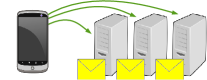
(a) The client sends a share of its encoded submission and SNIP proof to each server.

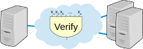
(b) The servers validate the client’s SNIP proof to ensure that the submission is valid.

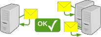
(c) If the checks pass, the servers update their local accumulators with the client-provided data.

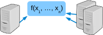
(d) After accumulating many packets, the servers publish their accumulators to reveal the aggregate.

Figure 1: An overview of the Prio pipeline for processing client submissions.

                  

Let us introduce Prio by first presenting a simplified version of it. In this simple version, each client holds a one-bit integer $x_{i}$ and the servers want to compute the sum of the clients’ private values $\sum_{i}x_{i}$. Even this very basic functionality has many real-world applications. For example, the developer of a health data mobile app could use this scheme to collect the number of app users who have a certain medical condition. In this application, the bit $x_{i}$ would indicate whether the user has the condition, and the sum over the $x_{i}$s gives the count of affected users.

The public parameters for the Prio deployment include a prime $p$. Throughout this paper, when we write “$c=a+b\in\mathbb{F}_{p}$,” we mean “$c=a+b\pmod{p}$.” The simplified Prio scheme for computing sums proceeds in three steps:

1. Upload. Each client $i$ splits its private value $x_{i}$ into $s$ shares, one per server, using a secret-sharing scheme. In particular, the client picks random integers $[x_{i}]_{1},\dots,[x_{i}]_{s}\in\mathbb{F}_{p}$, subject to the constraint: $x_{i}=[x_{i}]_{1}+\cdots+[x_{i}]_{s}\in\mathbb{F}_{p}$. The client then sends, over an encrypted and authenticated channel, one share of its submission to each server.

2. Aggregate. Each server $j$ holds an accumulator value $A_{j}\in\mathbb{F}_{p}$, initialized to zero. Upon receiving a share from the $i$th client, the server adds the uploaded share into its accumulator: $A_{j}\leftarrow A_{j}+[x_{i}]_{j}\in\mathbb{F}_{p}$.

3. Publish. Once the servers have received a share from each client, they publish their accumulator values. Computing the sum of the accumulator values $\sum_{j}A_{j}\in\mathbb{F}_{p}$ yields the desired sum $\sum_{i}x_{i}$ of the clients’ private values, as long as the modulus $p$ is larger than the number of clients (i.e., the sum $\sum_{i}x_{i}$ does not “overflow” the modulus).

There are two observations we can make about this scheme. First, even this simple scheme provides privacy: the servers learn the sum $\sum_{i}x_{i}$ but they learn nothing else about the clients’ private inputs. Second, the scheme does not provide robustness. A single malicious client can completely corrupt the protocol output by submitting (for example), a random integer $r\in\mathbb{F}_{p}$ to each server.

The core contributions of Prio are to improve this basic scheme in terms of security and functionality. In terms of security, Prio extends the simple scheme to provide robustness in the face of malicious clients. In terms of functionality, Prio extends the simple scheme to allow privacy-preserving computation of a wide array of aggregation functions (not just sum).

4 Protecting correctness with SNIPs

Upon receiving shares of a client’s data value, the Prio servers need a way to check if the client-submitted value is well formed. For example, in the simplified protocol of Section 3, every client is supposed to send the servers the share of a value $x$ such that $0\leq x\leq 1$. However, since the client sends only a single share of its value $x$ to each server—to preserve privacy—each server essentially receives an encrypted version of $x$ and cannot unilaterally determine if $x$ is well formed. In the more general setting, each Prio client submits to each server a share $[x]_{i}$ of a vector $x\in\mathbb{F}^{L}$, for some finite field $\mathbb{F}$. The servers hold a validation predicate $\textsf{Valid}(\cdot)$, and should only accept the client’s data submission if $\textsf{Valid}(x)=1$ (Figure 1a).

To execute this check in Prio, we introduce a new cryptographic tool called secret-shared non-interactive proofs (“SNIPs”). With these proofs, the client can quickly prove to the servers that $\textsf{Valid}(x)=1$, for an arbitrary function Valid, without leaking anything else about $x$ to the servers.

Building blocks.

All arithmetic in this section takes place in a finite field $\mathbb{F}$, or modulo a prime $p$, if you prefer. We use a simple additive secret-sharing scheme over $\mathbb{F}$: to split a value $x\in\mathbb{F}$ into $s$ shares, choose random values $([x]_{1},\dots,[x]_{s})\in\mathbb{F}^{s}$ subject to the constraint that $x=\sum_{i}[x]_{i}\in\mathbb{F}$. In our notation, $[x]_{i}$ denotes the $i$th share of $x$. An adversary who gets hold of any subset of up to $s-1$ shares of $x$ learns nothing, in an information-theoretic sense, about $x$ from the shares.

This secret-sharing scheme is linear, which means that the servers can perform affine operations on shares without communicating. That is, by adding shares $[x]_{i}$ and $[y]_{i}$, the servers can locally construct shares $[x+y]_{i}$. Given a share $[x]_{i}$, the servers can also construct shares $[\alpha x+\beta]_{i}$, for any constants $\alpha,\beta\in\mathbb{F}$. (This is a classic observation from the multi-party computation literature [15].)

Our construction uses arithmetic circuits. An arithmetic circuit is like a boolean circuit except that it uses finite-field multiplication, addition, and multiplication-by-constant gates, instead of boolean and, or, and not gates. See Appendix C.1 for a formal definition.

4.1 Overview

A secret-shared non-interactive proof (SNIP) protocol consists of an interaction between a client (the prover) and multiple servers (the verifiers). At the start of the protocol:

• each server $i$ holds a vector $[x]_{i}\in\mathbb{F}^{L}$,

• the client holds the vector $x=\sum_{i}[x]_{i}\in\mathbb{F}^{L}$, and

• all parties hold an arithmetic circuit representing a predicate $\textsf{Valid}:\mathbb{F}^{L}\to\mathbb{F}$.

The client’s goal is to convince the servers that $\textsf{Valid}(x)=1$, without leaking anything else about $x$ to the servers. To do so, the client sends a proof string to each server. After receiving these proof strings, the servers gossip amongst themselves and then conclude either that $\textsf{Valid}(x)=1$ (the servers “accept $x$”) or not (the servers “reject $x$”).

For a SNIP to be useful in Prio, it must satisfy the following properties:

Correctness.

If all parties are honest, the servers will accept $x$.

Soundness.

If all servers are honest, and if $\textsf{Valid}(x)\neq 1$, then for all malicious clients, even ones running in super-polynomial time, the servers will reject $x$ with overwhelming probability. In other words, no matter how the client cheats, the servers will almost always reject $x$.

Zero knowledge.

If the client and at least one server are honest, then the servers learn nothing about $x$, except that $\textsf{Valid}(x)=1$. More precisely, there exists a simulator (that does not take $x$ as input) that accurately reproduces the view of any proper subset of malicious servers executing the SNIP protocol.

See Appendix D for formal definitions.

These three security properties are nearly identical to the properties required of a zero-knowledge interactive proof system [70]. However, in the conventional zero-knowledge setting, there is a single prover and single verifier, whereas here we have a single prover (the client) and many verifiers (the servers).

Our contribution. We devise a SNIP that requires minimal server-to-server communication, is compatible with any public Valid circuit, and relies solely on fast, information-theoretic primitives. (We discuss how to hide the Valid circuit from the client in Section 4.4.)

To build the SNIP, we first generalize a “batch verification” technique of Ben-Sasson et al. [19] and then show how a set of servers can use it to verify an entire circuit computation by exchanging a only few field elements. We implement this last step with a new adaptation of Beaver’s multi-party computation (MPC) protocol to the client/server setting [9].

Related techniques. Prior work has studied interactive proofs in both the many-prover [14, 60] and many-verifier settings [10, 1]. Prior many-verifier protocols require relatively expensive public-key primitives [1] or require an amount of server-to-server traffic that grows linearly in the size of the circuit for the Valid function [10]. In concurrent independent work, Boyle et al. [25] construct what we can view as a very efficient SNIP for a specific Valid function, in which the servers are semi-honest (“honest but curious”) [25]. They also use a Beaver-style MPC multiplication; their techniques otherwise differ from ours.

4.2 Constructing SNIPs

To run the SNIP protocol, the client and servers execute the following steps:

Set-up. Let $M$ be the number of multiplication gates in the arithmetic circuit for Valid. We work over a field $\mathbb{F}$ that is large enough to ensure that $2M+2\ll|\mathbb{F}|$.

Step 1: Client evaluation.

The client evaluates the Valid circuit on its input $x$. The client thus knows the value that every wire in the circuit takes on during the computation of $\textsf{Valid}(x)$. The client uses these wire values to construct three randomized polynomials $f$, $g$, and $h$, which encode the values on the input and output wires of each of the $M$ multiplication gates in the $\textsf{Valid}(x)$ computation.

Label the $M$ multiplication gates in the $\textsf{Valid}(x)$ circuit, in topological order from inputs to outputs, with the numbers $\{1,\dots,M\}$. For $t\in\{1,\dots,M\}$, let us define $u_{t}$ and $v_{t}$ to be the values on the left and right input wires of the $t$-th multiplication gate. The client chooses $u_{0}$ and $v_{0}$ to be values sampled independently and uniformly at random from $\mathbb{F}$. Then, define $f$ and $g$ to be the lowest-degree polynomials such that $f(t)=u_{t}$ and $g(t)=v_{t}$, for all $t\in\{0,\dots,M\}$. Finally, define the polynomial $h$ as ${h=f\cdot g}$.

The polynomials $f$ and $g$ will have degree at most $M$, and the polynomial $h$ will have degree at most $2M$. Since $h(t)=f(t)\cdot g(t)=u_{t}\cdot v_{t}$ for all $t\in\{1,\dots,M\}$, $h(t)$ is equal to the value of the output wire ($u_{t}\cdot v_{t}$) of the $t$-th multiplication gate in the $\textsf{Valid}(x)$ circuit, for $1\leq t\leq M$.

In Step 4.2 of the checking protocol, the client executes the computation of $\textsf{Valid}(x)$, uses polynomial interpolation to construct the polynomials $f$ and $g$, and multiplies these polynomials to produce $h=f\cdot g$. The client then splits the random values $f(0)=u_{0}$ and $g(0)=v_{0}$, using additive secret sharing, and send shares $[f(0)]_{i}$ and $[g(0)]_{i}$ to server $i$. The client also splits the coefficients of $h$ and sends the $i$th share of the coefficients $[h]_{i}$ to server $i$.

Step 2: Consistency checking at the servers.

Each server $i$ holds a share $[x]_{i}$ of the client’s private value $x$. Each server also holds shares $[f(0)]_{i}$, $[g(0)]_{i}$, and $[h]_{i}$. Using these values, each server can—without communicating with the other servers—produce shares $[f]_{i}$ and $[g]_{i}$ of the polynomials $f$ and $g$.

To see how, first observe that if a server has a share of every wire value in the circuit, along with shares of $f(0)$ and $g(0)$, it can construct $[f]_{i}$ and $[g]_{i}$ using polynomial interpolation. Next, realize that each server can reconstruct a share of every wire value in the circuit since each server:

• has a share of each of the input wire values ($[x]_{i}$),

• has a share of each wire value coming out of a multiplication gate (for $t\in\{1,\dots,M\}$, the value $[h]_{i}(t)$ is a share of the $t$-th such wire), and

• can derive all other wire value shares via affine operations on the wire value shares it already has.

Using these wire value shares, the servers use polynomial interpolation to construct $[f]_{i}$ and $[g]_{i}$.

If the client and servers have acted honestly up to this point, then the servers will now hold shares of polynomials $f$, $g$, and $h$ such that $f\cdot g=h$.

In contrast, a malicious client could have sent the servers shares of a polynomial $\hat{h}$ such that, for some $t\in\{1,\dots,M\}$, $\hat{h}(t)$ is not the value on the output wire in the $t$-th multiplication gate of the $\textsf{Valid}(x)$ computation. In this case, the servers will reconstruct shares of polynomials $\hat{f}$ and $\hat{g}$ that might not be equal to $f$ and $g$. We will then have with certainty that $\hat{h}\neq\hat{f}\cdot\hat{g}$. To see why, consider the least $t_{0}$ for which $\hat{h}(t_{0})\neq h(t_{0})$. For all $t\leq t_{0}$, $\hat{f}(t)=f(t)$ and $\hat{g}(t)=g(t)$, by construction. Since

$$\hat{h}(t_{0})\neq h(t_{0})=f(t_{0})\cdot g(t_{0})=\hat{f}(t_{0})\cdot\hat{g}(t_{0}),$$

it must be that $\hat{h}(t_{0})\neq\hat{f}(t_{0})\cdot\hat{g}(t_{0})$, so $\hat{h}\neq\hat{f}\cdot\hat{g}$. (Ben-Sasson et al. [19] use polynomial identities to check the consistency of secret-shared values in a very different MPC protocol. Their construction inspired our approach.)

Step 3a: Polynomial identity test.

At the start of this step, each server $i$ holds shares $[\hat{f}]_{i}$, $[\hat{g}]_{i}$, and $[\hat{h}]_{i}$ of polynomials $\hat{f}$, $\hat{g}$, and $\hat{h}$. Furthermore, it holds that $\hat{f}\cdot\hat{g}=\hat{h}$ if and only if the servers collectively hold a set of wire value shares that, when summed up, equal the internal wire values of the $\textsf{Valid}(x)$ circuit computation.

The servers now execute a variant of the Schwartz-Zippel randomized polynomial identity test [104, 126] to check whether this relation holds. The principle of the test is that if $\hat{f}(t)\cdot\hat{g}(t)\neq\hat{h}(t)$, then the polynomial $t\cdot(\hat{f}(t)\cdot\hat{g}(t)-\hat{h}(t))$ is a non-zero polynomial of degree at most $2M+1$. (Multiplying the polynomial $\hat{f}\cdot g-\hat{h}$ by $t$ is useful for the next step.) Such a polynomial can have at most $2M+1$ zeros in $\mathbb{F}$, so if we choose a random $r\in\mathbb{F}$ and evaluate $r\cdot(\hat{f}(r)\cdot\hat{g}(r)-\hat{h}(r))$, the servers will detect that $\hat{f}\cdot\hat{g}\neq\hat{h}$ with probability at least $1-\frac{2M+1}{|\mathbb{F}|}$.

To execute the polynomial identity test, one of the servers samples a random value $r\in\mathbb{F}$. Each server $i$ then evaluates her share of each of the three polynomials on the point $r$ to get $[\hat{f}(r)]_{i}$, $[\hat{g}(r)]_{i}$, and $[\hat{h}(r)]_{i}$. The servers can perform this step locally, since polynomial evaluation requires only affine operations on shares. Each server then applies a local linear operation to these last two shares to produce shares of $[r\cdot\hat{g}(r)]_{i}$, and ${[r\cdot\hat{h}(r)]_{i}}$.

Assume for a moment that each server $i$ can multiply her shares $[\hat{f}(r)]_{i}$ and $[r\cdot\hat{g}(r)]_{i}$ to produce a share ${[r\cdot\hat{f}(r)\cdot\hat{g}(r)]_{i}}$. In this case, the servers can use a linear operation to get shares $\sigma_{i}=[r\cdot(\hat{f}(r)\cdot\hat{g}(r)-\hat{h}(r))]_{i}$. The servers then publish these $\sigma_{i}$s and ensure that ${\sum_{i}\sigma_{i}=0\in\mathbb{F}}$. The servers reject the client’s submission if $\sum_{i}\sigma_{i}\neq 0$.

Step 4.2b: Multiplication of shares.

Finally, the servers must somehow multiply their shares $[\hat{f}(r)]_{i}$ and $[r\cdot\hat{g}(r)]_{i}$ to get a share $[r\cdot\hat{f}(r)\cdot\hat{g}(r)]_{i}$ without leaking anything to each other about the values $\hat{f}(r)$ and $\hat{g}(r)$. To do so, we adapt a multi-party computation (MPC) technique of Beaver [9]. The details of Beaver’s MPC protocol are not critical here, but we include them for reference in Appendix C.2.

Beaver’s result implies that if servers receive, from a trusted dealer, one-time-use shares $([a]_{i},[b]_{i},[c]_{i})\in\mathbb{F}^{3}$ of random values such that $a\cdot b=c\in\mathbb{F}$ (“multiplication triples”), then the servers can very efficiently execute a multi-party multiplication of a pair secret-shared values. Furthermore, the multiplication protocol is fast: it requires each server to broadcast a single message.

In the traditional MPC setting, the parties to the computation have to run an expensive cryptographic protocol to generate the multiplication triples themselves [46]. In our setting however, the client generates the multiplication triple on behalf of the servers: the client chooses $(a,b,c)\in\mathbb{F}^{3}$ such that $a\cdot b=c\in\mathbb{F}$, and sends shares of these values to each server. If the client produces shares of these values correctly, then the servers can perform a multi-party multiplication of shares to complete the correctness check of the prior section.

Crucially, we can ensure that even if the client sends shares of an invalid multiplication triple to the servers, the servers will still catch the cheating client with high probability. First, say that a cheating client sends the servers shares $([a]_{i},[b]_{i},[c]_{i})\in\mathbb{F}^{3}$ such that $a\cdot b\neq c\in\mathbb{F}$. Then we can write $a\cdot b=(c+\alpha)\in\mathbb{F}$, for some constant $\alpha>0$.

In this case, when the servers run Beaver’s MPC multiplication protocol to execute the polynomial identity test, the result of the test will be shifted by $\alpha$. (To confirm this, consult our summary of Beaver’s protocol in Appendix C.2.) So the servers will effectively testing whether the polynomial

$$\hat{P}(t)=t\cdot(\hat{f}(t)\cdot\hat{g}(t)-\hat{h}(t))+\alpha$$

is identically zero. Whenever $\hat{f}\cdot\hat{g}\neq\hat{h}$, it holds that $t\cdot(\hat{f}(t)\cdot\hat{g}(t)-\hat{h}(t))$ is a non-zero polynomial. So, if ${\hat{f}\cdot\hat{g}\neq\hat{h}}$, then $\hat{P}(t)$ must also be a non-zero polynomial. (In constructing $\hat{P}$, We multiply the term “${\hat{f}\cdot\hat{g}-\hat{h}}$” by $t$, to ensure that whenever this expression is non-zero, the resulting polynomial $\hat{P}$ is non-zero, even if $\hat{f}$, $\hat{g}$, and $\hat{h}$ are degree-zero polynomials, and the client chooses $\alpha$ adversarially.)

Since we only require soundness to hold if all servers are honest, we may assume that the client did not know the servers’ random value $r$ when the client generated its multiplication triple. This implies that $r$ is distributed independently of $\alpha$, and since we only require soundness to hold if the servers are honest, we may assume that $r$ is sampled uniformly from $\mathbb{F}$ as well.

So, even if the client cheats, the servers will still be executing the polynomial identity test on a non-zero polynomial of degree at most $2M+1$. The servers will thus catch a cheating client with probability at least $1-\frac{2M+1}{|\mathbb{F}|}$. In Appendix D.1, we present a formal definition of the soundness property and we prove that it holds.

Step 4: Output verification.

If all servers are honest, at the start of the final step of the protocol, each server $i$ will hold a set of shares of the values that the Valid circuit takes on during computation of $\textsf{Valid}(x)$: $([w_{1}]_{i},[w_{2}]_{i},\dots)$. The servers already hold shares of the input wires of this circuit ($[x]_{i}$), so to confirm that $\textsf{Valid}(x)=1$, the servers need only publish their shares of the output wire. When they do, the servers can sum up these shares to confirm that the value on the output wire is equal to one, in which case it must be that $\textsf{Valid}(x)=1$, except with some small failure probability due to the polynomial identity test.

Combining all of the pieces above: each share of a SNIP proof consists of a share of the client-produced tuple ${\pi=(f(0),g(0),h,a,b,c)}$.

4.3 Security and efficiency

The correctness of the scheme follows by construction. To trick the servers into accepting a malformed submission, a cheating client must subvert the polynomial identity test. This bad event has probability at most $(2M+1)/|\mathbb{F}|$, where $M$ is the number of multiplication gates in $\textsf{Valid}(\cdot)$. By taking $|\mathbb{F}|\approx 2^{128}$, or repeating Step 4.2 a few times, we can make this failure probability extremely small.

We require neither completeness nor soundness to hold in the presence of malicious servers, though we do require soundness against malicious clients. A malicious server can thus trick the honest servers into rejecting a well-formed client submission that they should have accepted. This is tantamount to the malicious server mounting a selective denial-of-service attack against the honest client. We discuss this attack in Section 7.

We prove in Appendix D.2 that, as long as there is at least one honest server, the dishonest servers gain no information—in an unconditional, information-theoretic sense—about the client’s data values nor about the values on the internal wires in the $\textsf{Valid}(x)$ circuit.

		NIZK	SNARK	Prio (SNIP)
Client	Exps.	$M$	$M$	$0$
	Muls.	$0$	$M\log M$	$M\log M$
	Proof len.	$M$	$1$	$M$
Servers	Exps./Pairs.	$M$	$1$	$0$
	Muls.	$0$	$M$	$M\log M$
	Data transfer	$M$	$1$	$1$

Table 2: An asymptotic comparison of Prio with standard zero-knowledge techniques showing that Prio reduces the computational burden for clients and servers. The client holds a vector $x\in\mathbb{F}^{M}$, each server $i$ holds a share $[x]_{i}$, and the client convinces the servers that each component of $x$ is a $0/1$ value in $\mathbb{F}$. We suppress the $\Theta(\cdot)$ notation for readability.

Efficiency.

The remarkable property of this SNIP construction is that the server-to-server communication cost grows neither with the complexity of the verification circuit nor with the size of the value $x$ (Table 2). The computation cost at the servers is essentially the same as the cost for each server to evaluate the Valid circuit locally. That said, the client-to-server communication cost does grow linearly with the size of the Valid circuit. An interesting challenge would be to try to reduce the client’s bandwidth usage without resorting to relatively expensive public-key cryptographic techniques [97, 18, 17, 41, 26].

4.4 Computation at the servers

Constructing the SNIP proof requires the client to compute $\textsf{Valid}(x)$ on its own. If the verification circuit takes secret server-provided values as input, or is itself a secret belonging to the servers, then the client does not have enough information to compute $\textsf{Valid}(x)$. For example, the servers could run a proprietary verification algorithm to detect spammy client submissions—the servers would want to run this algorithm without revealing it to the (possibly spam-producing) clients. To handle this use case, the servers can execute the verification check themselves at a slightly higher cost.

This variant maintains privacy only against “honest but curious” servers—in contrast, the SNIP-based variant maintains privacy against actively malicious servers. See Appendix E for details.

5 Gathering complex statistics

So far, we have developed the means to compute private sums over client-provided data (Section 3) and to check an arbitrary validation predicate against secret-shared data (Section 4). Combining these two ideas with careful data encodings, which we introduce now, allows Prio to compute more sophisticated statistics over private client data. At a high level, each client first encodes its private data value in a prescribed way, and the servers then privately compute the sum of the encodings. Finally, the servers can decode the summed encodings to recover the statistic of interest. The participants perform this encoding and decoding via a mechanism we call affine-aggregatable encodings (“AFEs”).

5.1 Affine-aggregatable encodings (AFEs)

In our setting, each client $i$ holds a value $x_{i}\in\mathcal{D}$, where $\mathcal{D}$ is some set of data values. The servers hold an aggregation function $f:\mathcal{D}^{n}\to\mathcal{A}$, whose range is a set of aggregates $\mathcal{A}$. For example, the function $f$ might compute the standard deviation of its $n$ inputs. The servers’ goal is to evaluate $f(x_{1},\ldots,x_{n})$ without learning the $x_{i}$s.

An AFE gives an efficient way to encode the data values $x_{i}$ such that it is possible to compute the value $f(x_{1},\dots,x_{n})$ given only the sum of the encodings of $x_{1},\ldots,x_{n}$. An AFE consists of three efficient algorithms $(\textsf{Encode},\textsf{Valid},\textsf{Decode})$, defined with respect to a field $\mathbb{F}$ and two integers $k$ and $k^{\prime}$, where $k^{\prime}\leq k$:

• $\textsf{Encode}(x)$: maps an input $x\in\mathcal{D}$ to its encoding in $\mathbb{F}^{k}$,

• $\textsf{Valid}(y)$: returns true if and only if $y\in\mathbb{F}^{k}$ is a valid encoding of some data item in $\mathcal{D}$,

• $\textsf{Decode}(\sigma)$: takes $\sigma=\sum_{i=1}^{n}\textsf{Trunc}_{k^{\prime}}\big{(}\textsf{Encode}(x_{i})\big{)}\in\mathbb{F}^{k^{\prime}}$ as input, and outputs $f(x_{1},\dots,x_{n})$. The $\textsf{Trunc}_{k^{\prime}}(\cdot)$ function outputs the first $k^{\prime}\leq k$ components of its input.

The AFE uses all $k$ components of the encoding in validation, but only uses $k^{\prime}$ components to decode $\sigma$. In many of our applications we have $k^{\prime}=k$.

An AFE is private with respect to a function $\hat{f}$, or simply $\hat{f}$-private, if $\sigma$ reveals nothing about $x_{1},\ldots,x_{n}$ beyond what $\hat{f}(x_{1},\dots,x_{n})$ itself reveals. More precisely, it is possible to efficiently simulate $\sigma$ given only $\hat{f}(x_{1},\dots,x_{n})$. Usually $\hat{f}$ reveals nothing more than the aggregation function $f$ (i.e., the minimum leakage possible), but in some cases $\hat{f}$ reveals a little more than $f$.

For some functions $f$ we can build more efficient $f$-private AFEs by allowing the encoding algorithm to be randomized. In these cases, we allow the decoding algorithm to return an answer that is only an approximation of $f$, and we also allow it to fail with some small probability.

Prior systems have made use of specific AFEs for sums [56, 86], standard deviations [100], counts [92, 28], and least-squares regression [82]. Our contribution is to unify these notions and to adopt existing AFEs to enable better composition with Prio’s SNIPs. In particular, by using more complex encodings, we can reduce the size of the circuit for Valid, which results in shorter SNIP proofs.

AFEs in Prio: Putting it all together.

The full Prio system computes $f(x_{1},\ldots,x_{n})$ privately as follows (see Figure 1a): Each client encodes its data value $x$ using the AFE Encode routine for the aggregation function $f$. Then, as in the simple scheme of Section 3, every client splits its encoding into $s$ shares and sends one share to each of the $s$ servers. The client uses a SNIP proof (Section 4) to convince the servers that its encoding satisfies the AFE Valid predicate.

Upon receiving a client’s submission, the servers verify the SNIP to ensure that the encoding is well-formed. If the servers conclude that the encoding is valid, every server adds the first $k^{\prime}$ components of the encoding share to its local running accumulator. (Recall that $k^{\prime}$ is a parameter of the AFE scheme.) Finally, after collecting valid submissions from many clients, every server publishes its local accumulator, enabling anyone to run the AFE Decode routine to compute the final statistic in the clear. The formal description of the system is presented in Appendix H, where we also analyze its security.

Limitations. There exist aggregation functions for which all AFE constructions must have large encodings. For instance, say that each of $n$ clients holds an integer $x_{i}$, where $1\leq x_{i}\leq n$. We might like an AFE that computes the median of these integers $\{x_{1},\dots,x_{n}\}$, working over a field $\mathbb{F}$ with $|\mathbb{F}|\approx n^{d}$, for some constant $d\geq 1$.

We show that there is no such AFE whose encodings consist of $k^{\prime}\in o(n/\log n)$ field elements. Suppose, towards a contradiction, that such an AFE did exist. Then we could describe any sum of encodings using at most $O(k^{\prime}\log|\mathbb{F}|)=o(n)$ bits of information. From this AFE, we could build a single-pass, space-$o(n)$ streaming algorithm for computing the exact median of an $n$-item stream. But every single-pass streaming algorithm for computing the exact median over an $n$-item stream requires $\Omega(n)$ bits of space [74], which is a contradiction. Similar arguments may rule out space-efficient AFE constructions for other natural functions.

5.2 Aggregating basic data types

This section presents the basic affine-aggregatable encoding schemes that serve as building blocks for the more sophisticated schemes. In the following constructions, the clients hold data values $x_{1},\dots,x_{n}\in\mathcal{D}$, and our goal is to compute an aggregate $f(x_{1},\dots,x_{n})$.

In constructing these encodings, we have two goals. The first is to ensure that the AFE leaks as little as possible about the $x_{i}$s, apart from the value $f(x_{1},\dots,x_{n})$ itself. The second is to minimize the number of multiplication gates in the arithmetic circuit for Valid, since the cost of the SNIPs grows with this quantity.

In what follows, we let $\lambda$ be a security parameter, such as $\lambda=80$ or $\lambda=128$.

Integer sum and mean.

We first construct an AFE for computing the sum of $b$-bit integers. Let $\mathbb{F}$ be a finite field of size at least $n2^{b}$. On input $0\leq x\leq 2^{b}-1$, the $\textsf{Encode}(x)$ algorithm first computes the bit representation of $x$, denoted $(\beta_{0},\beta_{1},\dots,\beta_{b-1})\in\{0,1\}^{b}$. It then treats the binary digits as elements of $\mathbb{F}$, and outputs

$$\textsf{Encode}(x)=(x,\beta_{0},\ldots,\beta_{b-1})\in\mathbb{F}^{b+1}.$$

To check that $x$ represents a $b$-bit integer, the Valid algorithm ensures that each $\beta_{i}$ is a bit, and that the bits represent $x$. Specifically, the algorithm checks that the following equalities hold over $\mathbb{F}$:

$$\textsf{Valid}(\textsf{Encode}(x))=\bigg{(}x=\sum_{i=0}^{b-1}2^{i}\beta_{i}\bigg{)}\land\bigwedge_{i=1}^{n}\bigg{[}(\beta_{i}-1)\cdot\beta_{i}=0\bigg{]}.$$

The Decode algorithm takes the sum of encodings $\sigma$ as input, truncated to only the first coordinate. That is, $\sigma=\sum_{i=1}^{n}\textsf{Trunc}_{1}\big{(}\textsf{Encode}(x_{1})\big{)}=x_{1}+\cdots+x_{n}$. This $\sigma$ is the required aggregate output. Moreover, this AFE is clearly sum-private.

To compute the arithmetic mean, we divide the sum of integers by $n$ over the rationals. Computing the product and geometric mean works in exactly the same matter, except that we encode $x$ using $b$-bit logarithms.

Variance and stddev.

Using known techniques [30, 100], the summation AFE above lets us compute the variance of a set of $b$-bit integers using the identity: $\text{Var}(X)=\text{E}[X^{2}]-(\text{E}[X])^{2}$. Each client encodes its integer $x$ as $(x,x^{2})$ and then applies the summation AFE to each of the two components. (The Valid algorithm also ensures that second integer is the square of the first.) The resulting two values let us compute the variance.

This AFE also reveals the expectation $\text{E}[X]$. It is private with respect to the function $\hat{f}$ that outputs both the expectation and variance of the given set of integers.

Boolean or and and.

When $\mathcal{D}=\{0,1\}$ and $f(x_{1},\ldots,x_{n})=\textsc{or}(x_{1},\ldots,x_{n})$ the encoding operation outputs an element of $\mathbb{F}_{2}^{\lambda}$ (i.e., a $\lambda$-bit bitstring) as:

$$\textsf{Encode}(x)=\begin{cases}\text{$\lambda$ zeros}&\text{if $x=0$}\\ \text{a random element in $\mathbb{F}_{2}^{\lambda}$}&\text{if $x=1$.}\end{cases}$$

The Valid algorithm outputs “1” always, since all $\lambda$-bit encodings are valid. The sum of encodings is simply the xor of the $n$ $\lambda$-bit encodings. The Decode algorithm takes as input a $\lambda$-bit string and outputs “0” if and only if its input is a $\lambda$-bit string of zeros. With probability $1-2^{-\lambda}$, over the randomness of the encoding algorithm, the decoding operation returns the boolean or of the encoded values. This AFE is or-private. A similar construction yields an AFE for boolean and.

min and max.

To compute the minimum and maximum of integers over a range $\{0,\dots,B-1\}$, where $B$ is small (e.g., car speeds in the range $0$–$250$ km/h), the Encode algorithm can represent each integer in unary as a length-$B$ vector of bits $(\beta_{0},\dots,\beta_{B-1})$, where $\beta_{i}=1$ if and only if the client’s value $x\leq i$. We can use the bitwise-or construction above to take the or of the client-provided vectors—the largest value containing a “1” is the maximum. To compute the minimum instead, replace or with and. This is min-private, as in the or protocol above.

When the domain is large (e.g., we want the max of 64-bit packet counters, in a networking application), we can get a $c$-approximation of the min and max using a similar idea: divide the range $\{0,\dots,B-1\}$ into $b=\log_{c}B$ “bins” $[0,c),[c,c^{2}),\dots,[c^{b-1},B)$. Then, use the small-range min/max construction, over the $b$ bins, to compute the approximate statistic. The output will be within a multiplicative factor of $c$ of the true value. This construction is private with respect to the approximate min/max function.

Frequency count.

Here, every client has a value $x$ in a small set of data values $\mathcal{D}=\{0,\dots,B-1\}$. The goal is to output a $B$-element vector $v$, where $v[i]$ is the number of clients that hold the value $i$, for every $0\leq i<B$.

Let $\mathbb{F}$ be a field of size at least $n$. The Encode algorithm encodes a value $x\in\mathcal{D}$ as a length-$B$ vector $(\beta_{0},\dots,\beta_{B-1})\in\mathbb{F}^{B}$ where $\beta_{i}=1$ if $x=i$ and $\beta_{i}=0$ otherwise. The Valid algorithm checks that each $\beta$ value is in the set $\{0,1\}$ and that the sum of the $\beta$s is exactly one. The Decode algorithm does nothing: the final output is a length-$B$ vector, whose $i$th component gives the number of clients who took on value $i$. Again, this AFE is private with respect to the function being computed.

The output of this AFE yields enough information to compute other useful functions (e.g., quantiles) of the distribution of the clients’ $x$ values. When the domain $\mathcal{D}$ is large, this AFE is very inefficient. In Appendix G, we give AFEs for approximate counts over large domains.

Sets.

We can compute the intersection or union of sets over a small universe of elements using the boolean AFE operations: represent a set of $B$ items as its characteristic vector of booleans, and compute an and for intersection and an or for union. When the universe is large, the approximate AFEs of Appendix G are more efficient.

5.3 Machine learning

We can use Prio for training machine learning models on private client data. To do so, we exploit the observation of Karr et al. [82] that a system for computing private sums can also privately train linear models. (In Appendix G, we also show how to use Prio to privately evaluate the $R^{2}$-coefficient of an existing model.) In Prio, we extend their work by showing how to perform these tasks while maintaining robustness against malicious clients.

Suppose that every client holds a data point $(x,y)$ where $x$ and $y$ are $b$-bit integers. We would like to train a model that takes $x$ as input and outputs a real-valued prediction $\hat{y}_{i}=M(x)\in\mathbb{R}$ of $y$. We might predict a person’s blood pressure ($y$) from the number of steps they walk daily ($x$).

		Workstation		Phone
Field size:		$87$-bit	$265$-bit	$87$-bit	$265$-bit
Mul. in field ($\mu{}s$)		$1.013$	$1.485$	$11.218$	$14.930$
Prio client time	$L=10^{1}$	$0.003$	$0.004$	$0.017$	$0.024$
	$L=10^{2}$	$0.024$	$0.036$	$0.112$	$0.170$
	$L=10^{3}$	$0.221$	$0.344$	$1.059$	$2.165$

Table 3: Time in seconds for a client to generate a Prio submission of $L$ four-bit integers to be summed at the servers. Averaged over eight runs.

We wish to compute the least-squares linear fit $h(x)=c_{0}+c_{1}x$ over all of the client points. With $n$ clients, the model coefficients $c_{0}$ and $c_{1}$ satisfy the linear relation:

$$\begin{pmatrix}n&\sum_{i=1}^{n}x_{i}\\[5.69054pt] \sum_{i=1}^{n}x_{i}&\sum_{i=1}^{n}x_{i}^{2}\end{pmatrix}\cdot\begin{pmatrix}c_{0}\\[5.69054pt] c_{1}\end{pmatrix}=\begin{pmatrix}\sum_{i=1}^{n}y_{i}\\[5.69054pt] \sum_{i=1}^{n}x_{i}y_{i}\end{pmatrix}$$ (1)

To compute this linear system in an AFE, every client encodes her private point $(x,y)$ as a vector

$$(x,x^{2},y,xy,\quad\beta_{0},\ldots,\beta_{b-1},\quad\gamma_{0},\ldots,\gamma_{b-1})\in\mathbb{F}^{2b+4},$$

where $(\beta_{0},\ldots,\beta_{b-1})$ is the binary representation of $x$ and $(\gamma_{0},\ldots,\gamma_{b-1})$ is the binary representation of $y$. The validation algorithm checks that all the $\beta$ and $\gamma$ are in $\{0,1\}$, and that all the arithmetic relations hold, analogously to the validation check for the integer summation AFE. Finally, the decoding algorithm takes as input the sum of the encoded vectors truncated to the first four components:

$$\sigma=\textstyle{\big{(}\ \sum_{i=1}^{n}x,\quad\sum_{i=1}^{n}x^{2},\quad\sum_{i=1}^{n}y,\quad\sum_{i=1}^{n}xy\ \big{)}},$$

from which the decoding algorithm computes the required real regression coefficients $c_{0}$ and $c_{1}$ using (1). This AFE is private with respect to the function that outputs the least-squares fit $h(x)=c_{0}+c_{1}x$, along with the mean and variance of the set $\{x_{1},\ldots,x_{n}\}$.

When $x$ and $y$ are real numbers, we can embed the reals into a finite field $\mathbb{F}$ using a fixed-point representation, as long as we size the field large enough to avoid overflow.

The two-dimensional approach above generalizes directly to perform linear regression on $d$-dimensional feature vectors $\bar{x}=(x^{(1)},\ldots,x^{(d)})$. The AFE yields a least-squares approximation of the form $h(\bar{x})=c_{0}+c_{1}x^{(1)}+\cdots+c_{d}x^{(d)}$. The resulting AFE is private with respect to a function that reveals the least-square coefficients $(c_{0},\ldots,c_{d})$, along with the $d\times d$ covariance matrix $\sum_{i}{\bar{x}_{i}\cdot(\bar{x}_{i})^{T}}$.

6 Evaluation

In this section, we demonstrate that Prio’s theoretical contributions translate into practical performance gains. We have implemented a Prio prototype in 5,700 lines of Go and 620 lines of C (for FFT-based polynomial operations, built on the FLINT library [59]). Unless noted otherwise, our evaluations use an FFT-friendly 87-bit field. Our servers communicate with each other using Go’s TLS implementation. Clients encrypt and sign their messages to servers using NaCl’s “box” primitive, which obviates the need for client-to-server TLS connections. Our code is available online at https://crypto.stanford.edu/prio/.

We evaluate the SNIP-based variant of Prio (Section 4.1) and also the variant in which the servers keep the Valid predicate private (“Prio-MPC,” Section 4.4). Our implementation includes three optimizations described in Appendix I. The first uses a pseudo-random generator (e.g., AES in counter mode) to reduce the client-to-server data transfer by a factor of roughly $s$ in an $s$-server deployment. The second optimization allows the servers to verify SNIPs without needing to perform expensive polynomial interpolations. The third optimization gives an efficient way for the servers to compute the logical-and of multiple arithmetic circuits to check that multiple Valid predicates hold simultaneously.

Figure 4: Prio’s SNIPs provide the robustness guarantees of zero-knowledge proofs at 20-50$\times$ less cost.

Figure 5: Prio is insensitive to the number of aggregation servers.

Figure 6: Prio’s use of SNIPs (§4) reduces bandwidth consumption.

We compare Prio against a private aggregation scheme that uses non-interactive zero-knowledge proofs (NIZKs) to provide robustness. This protocol is similar to the “cryptographically verifiable” interactive protocol of Kursawe et al. [86] and has roughly the same cost, in terms of exponentiations per client request, as the “distributed decryption” variant of PrivEx [56]. We implement the NIZK scheme using a Go wrapper of OpenSSL’s NIST P256 code [50]. We do not compare Prio against systems, such as ANONIZE [76] and PrivStats [100], that rely on an external anonymizing proxy to protect against a network adversary. (We discuss this related work in Section 8.)

6.1 Microbenchmarks

Table 3 presents the time required for a Prio client to encode a data submission on a workstation (2.4 GHz Intel Xeon E5620) and mobile phone (Samsung Galaxy SIII, 1.4 GHz Cortex A9). For a submission of 100 integers, the client time is roughly 0.03 seconds on a workstation, and just over 0.1 seconds on a mobile phone.

To investigate the load that Prio places on the servers, we configured five Amazon EC2 servers (eight-core c3.2xlarge machines, Intel Xeon E5-2680 CPUs) in five Amazon data centers (N. Va., N. Ca., Oregon, Ireland, and Frankfurt) and had them run the Prio protocols. An additional three c3.2xlarge machines in the N. Va. data center simulated a large number of Prio clients. To maximize the load on the servers, we had each client send a stream of pre-generated Prio data packets to the servers over a single TCP connection. There is no need to use TLS on the client-to-server Prio connection because Prio packets are encrypted and authenticated at the application layer and can be replay-protected at the servers.

Figure 6 gives the throughput of this cluster in which each client submits a vector of zero/one integers and the servers sum these vectors. The “No privacy” line on the chart gives the throughput for a dummy scheme in which a single server accepts encrypted client data submissions directly from the clients with no privacy protection whatsoever. The “No robustness” line on the chart gives the throughput for a cluster of five servers that use a secret-sharing-based private aggregation scheme (à la Section 3) with no robustness protection. The five-server “No robustness” scheme is slower than the single-server “No privacy” scheme because of the cost of coordinating the processing of submissions amongst the five servers. The throughput of Prio is within a factor of 5$\times$ of the no-privacy scheme for many submission sizes, and Prio outperforms the NIZK-based scheme by more than an order of magnitude.

Figure 6 shows how the throughput of a Prio cluster changes as the number of servers increases, when the system is collecting the sum of 1,024 one-bit client-submitted integers, as in an anonymous survey application. For this experiment, we locate all of the servers in the same data center, so that the latency and bandwidth between each pair of servers is roughly constant. With more servers, an adversary has to compromise a larger number of machines to violate Prio’s privacy guarantees.

Figure 7: Client encoding time for different application domains when using Prio, a non-interactive zero-knowledge system (NIZK), or a SNARK-like system (estimated). Averaged over eight runs. The number of $\times$ gates in the Valid circuit is listed in parentheses.

Adding more servers barely affects the system’s throughput. The reason is that we are able to load-balance the bulk of the work of checking client submissions across all of the servers. (This optimization is only possible because we require robustness to hold only if all servers are honest.) We assign a single Prio server to be the “leader” that coordinates the checking of each client data submission. In processing a single submission in an $s$-server cluster, the leader transmits $s$ times more bits than a non-leader, but as the number of servers increases, each server is a leader for a smaller share of incoming submissions. The NIZK-based scheme also scales well: as the number of servers increases, the heavy computational load of checking the NIZKs is distributed over more machines.

Figure 6 shows the number of bytes each non-leader Prio server needs to transmit to check the validity of a single client submission for the two Prio variants, and for the NIZK scheme. The benefit of Prio is evident: the Prio servers transmit a constant number of bits per submission—independent of the size of the submission or complexity of the Valid routine. As the submitted vectors grow, Prio yields a 4,000-fold bandwidth saving over NIZKs, in terms of server data transfer.

6.2 Application scenarios

To demonstrate that Prio’s data types are expressive enough to collect real-world aggregates, we have configured Prio for a few potential application domains. Cell signal strength. A collection of Prio servers can collect the average mobile signal strength in each grid cell in a city without leaking the user’s location history to the aggregator. We divide the geographic area into a km² grid—the number of grid cells depends on the city’s size—and we encode the signal strength at the user’s present location as a four-bit integer. (If each client only submits signal-strength data for a few grid cells in each protocol run, extra optimizations can reduce the client-to-server data transfer. See “Share compression” in Appendix G.)

Browser statistics. The Chromium browser uses the RAPPOR system to gather private information about its users [57, 35]. We implement a Prio instance for gathering a subset of these statistics: average CPU and memory usage, along with the frequency counts of 16 URL roots. structure, described in Appendix G. We experiment with both low- and high-resolution parameters ($\delta=2^{-10}$, $\epsilon=1/10$; $\delta=2^{-20}$, $\epsilon=1/100$).

Health data modeling. We implement the AFE for training a regression model on private client data. We use the features from a preexisting heart disease data set (13 features of varying types: age, sex, cholesterol level, etc.) [78] and a breast cancer diagnosis data set (30 real-valued features using 14-bit fixed-point numbers) [120].

Anonymous surveys. We configure Prio to compute aggregates responses to sensitive surveys: we use the Beck Depression Inventory (21 questions on a 1-4 scale) [4], the Parent-Child Relationship Inventory (78 questions on a 1-4 scale) [63], and the California Psychological Inventory (434 boolean questions) [42].

Comparison to alternatives.

In Figure 7, we compare the computational cost Prio places on the client to the costs of other schemes for protecting robustness against misbehaving clients, when we configure the system for the aforementioned applications. The fact that a Prio client need only perform a single public-key encryption means that it dramatically outperforms schemes based on public-key cryptography. If the Valid circuit has $M$ multiplication gates, producing a discrete-log-based NIZK requires the client to perform $2M$ exponentiations (or elliptic-curve point multiplications). In contrast, Prio requires $O(M\log M)$ multiplications in a relatively small field, which is much cheaper for practical values of $M$.

Figure 8: Time for a client to encode a submission consisting of $d$-dimensional training example of 14-bit values for computing a private least-squares regression.

	No privacy	No robustness		Prio
$d$	Rate	Rate	Priv. cost	Rate	Robust. cost	Tot. cost
$2$	14,688	2,687	$5.5\times$	2,608	$1.0\times$	$\ \,\,5.6\times$
$4$	15,426	2,569	$6.0\times$	2,165	$1.2\times$	$\ \,\,7.1\times$
$6$	14,773	2,600	$5.7\times$	2,048	$1.3\times$	$\ \,\,7.2\times$
$8$	15,975	2,564	$6.2\times$	1,606	$1.6\times$	$\ \,\,9.5\times$
$10$	15,589	2,639	$5.9\times$	1,430	$1.8\times$	$10.9\times$
$12$	15,189	2,547	$6.0\times$	1,312	$1.9\times$	$11.6\times$

Table 9: The throughput, in client requests per second, of a global five-server cluster running a private $d$-dim. regression. We compare a scheme with no privacy, with privacy but no robustness, and Prio (with both).

In Figure 7, we give conservative estimates of the time required to generate a zkSNARK proof, based on timings of libsnark’s [18] implementation of the Pinocchio system [97] at the 128-bit security level. These proofs have the benefit of being very short: 288 bytes, irrespective of the complexity of the circuit. To realize the benefit of these succinct proofs, the statement being proved must also be concise since the verifier’s running time grows with the statement size. To achieve this conciseness in the Prio setting would require computing $sL$ hashes “inside the SNARK,” with $s$ servers and submissions of length $L$.

We optimistically estimate that each hash computation requires only 300 multiplication gates, using a subset-sum hash function [2, 17, 67, 77], and we ignore the cost of computing the Valid circuit in the SNARK. We then use the timings from the libsnark paper to arrive at the cost estimates. Each SNARK multiplication gate requires the client to compute a number of exponentiations, so the cost to the client is large, though the proof is admirably short.

6.3 Machine learning

Finally, we perform an end-to-end evaluation of Prio when the system is configured to train a $d$-dimensional least-squares regression model on private client-submitted data, in which each training example consists of a vector of 14-bit integers. These integers are large enough to represent vital health information, for example.

In Figure 8, we show the client encoding cost for Prio, along with the no-privacy and no-robustness schemes described in Section 6.1. The cost of Prio’s privacy and robustness guarantees amounts to roughly a 50$\times$ slowdown at the client over the no-privacy scheme due to the overhead of the SNIP proof generation. Even so, the absolute cost of Prio to the client is small—on the order of one tenth of a second.

Table 9 gives the rate at which the globally distributed five-server cluster described in Section 6.1 can process client submissions with and without privacy and robustness. The server-side cost of Prio is modest: only a 1-2$\times$ slowdown over the no-robustness scheme, and only a 5-15$\times$ slowdown over a scheme with no privacy at all. In contrast, the cost of robustness for the state-of-the-art NIZK schemes, per Figure 6, is closer to 100-200$\times$.

7 Discussion

Deployment scenarios.

Prio ensures client privacy as long as at least one server behaves honestly. We now discuss a number of deployment scenarios in which this assumption aligns with real-world incentives.

Tolerance to compromise. Prio lets an organization compute aggregate data about its clients without ever storing client data in a single vulnerable location. The organization could run all $s$ Prio servers itself, which would ensures data privacy against an attacker who compromises up to $s-1$ servers.

(a) RAPPOR [57] provides differential privacy [54] (not information-theoretic privacy) by adding random noise to client submissions.

(b) ANONIZE [76] and PrivStats [100] rely on an anonymizing proxy, such as Tor [51], to protect privacy against network eavesdroppers.

(c) Prio and other schemes using secret sharing [92, 56, 48, 86, 79, 30] offer ideal anonymity provided that the servers do not collude.

Figure 10: Comparison of techniques for anonymizing client data in private aggregation systems.

App store. A mobile application platform (e.g., Apple’s App Store or Google’s Play) can run one Prio server, and the developer of a mobile app can run the second Prio server. This allows the app developer to collect aggregate user data without having to bear the risks of holding these data in the clear.

Shared data. A group of $s$ organizations could use Prio to compute an aggregate over the union of their customers’ datasets, without learning each other’s private client data.

Private compute services. A large enterprise can contract with an external auditor or a non-profit (e.g., the Electronic Frontier Foundation) to jointly compute aggregate statistics over sensitive customer data using Prio.

Jurisdictional diversity. A multinational organization can spread its Prio servers across different countries. If law enforcement agents seize the Prio servers in one country, they cannot deanonymize the organization’s Prio users.

Common attacks.

Two general attacks apply to all systems, like Prio, that produce exact (un-noised) outputs while protecting privacy against a network adversary. The first attack is a selective denial-of-service attack. In this attack, the network adversary prevents all honest clients except one from being able to contact the Prio servers [105]. In this case, the protocol output is $f(x_{\text{honest}},x_{\text{evil}_{1}},\dots,x_{\text{evil}_{n}})$. Since the adversary knows the $x_{\text{evil}}$ values, the adversary could infer part or all of the one honest client’s private value $x_{\text{honest}}$.

In Prio, we deploy the standard defense against this attack, which is to have the servers wait to publish the aggregate statistic $f(x_{1},\dots,x_{n})$ until they are confident that the aggregate includes values from many honest clients. The best means to accomplish this will depend on the deployment setting.

One way is to have the servers keep a list of public keys of registered clients (e.g., the students enrolled at a university). Prio clients sign their submissions with the signing key corresponding to their registered public key and the servers wait to publish their accumulator values until a threshold number of registered clients have submitted valid messages. Standard defenses [125, 124, 114, 3] against Sybil attacks [52] would apply here.

The second attack is an intersection attack [83, 20, 122, 49]. In this attack, the adversary observes the output $f(x_{1},\dots,x_{n})$ of a run of the Prio protocol with $n$ honest clients. The adversary then forces the $n$th honest client offline and observes a subsequent protocol run, in which the servers compute $f(x^{\prime}_{1},\dots,x^{\prime}_{n-1})$. If the clients’ values are constant over time ($x_{i}=x^{\prime}_{i}$), then the adversary learns the difference $f(x_{1},\dots,x_{n})-f(x_{1},\dots,x_{n-1})$, which could reveal client $n$’s private value $x_{n}$ (e.g., if $f$ computes sum).

One way for the servers to defend against the attack is to add differential privacy noise to the results before publishing them [54]. Using existing techniques, the servers can add this noise in a distributed fashion to ensure that as long as at least one server is honest, no server sees the un-noised aggregate [55]. The definition of differential privacy ensures that computed statistics are distributed approximately the same whether or not the aggregate includes a particular client’s data. This same approach is also used in a system by Melis, Danezis, and De Cristofaro [92], which we discuss in Section 8.

Robustness against malicious servers.

Prio only provides robustness when all servers are honest. Providing robustness in the face of faulty servers is obviously desirable, but we are not convinced that it is worth the security and performance costs. Briefly, providing robustness necessarily weakens the privacy guarantees that the system provides: if the system protects robustness in the presence of $k$ faulty servers, then the system can protect privacy only against a coalition of at most $s-k-1$ malicious servers. We discuss this issue further in Appendix B.

8 Related Work

Private data-collection systems [56, 30, 48, 79, 86, 53, 92] that use secret-sharing based methods to compute sums over private user data typically (a) provide no robustness guarantees in the face of malicious clients, (b) use expensive NIZKs to prevent client misbehavior, or (c) fail to defend privacy against actively malicious servers [33].

Other data-collection systems have clients send their private data to an aggregator through a general-purpose anonymizing network, such as a mix-net [32, 47, 27, 87] or a DC-net [31, 110, 38, 39, 40]. These anonymity systems provide strong privacy properties, but require expensive “verifiable mixing” techniques [8, 95], or require work at the servers that is quadratic in the number of client messages sent through the system [38, 121].

PrivStats [100] and ANONIZE [76] outsource to Tor [51] (or another low-latency anonymity system [88, 61, 101]) the work of protecting privacy against a network adversary (Figure 10). Prio protects against an adversary that can see and control the entire network, while Tor-based schemes succumb to traffic-analysis attacks [94].

In data-collection systems based on differential privacy [54], the client adds structured noise to its private value before sending it to an aggregating server. The added noise gives the client “plausible deniability:” if the client sends a value $x$ to the servers, $x$ could be the client’s true private value, or it could be an unrelated value generated from the noise. Dwork et al. [55], Shi et al. [107], and Bassily and Smith [7] study this technique in a distributed setting, and the RAPPOR system [57, 58], deployed in Chromium, has put this idea into practice. A variant of the same principle is to have a trusted proxy (as in SuLQ [21] and PDDP [34]) or a set of minimally trusted servers [92] add noise to already-collected data.

The downside of these systems is that (a) if the client adds little noise, then the system does not provide much privacy, or (b) if the client adds a lot of noise, then low-frequency events may be lost in the noise [57]. Using server-added noise [92] ameliorates these problems.

In theory, secure multi-party computation (MPC) protocols [90, 123, 68, 15, 11] allow a set of servers, with some non-collusion assumptions, to privately compute any function over client-provided values. The generality of MPC comes with serious bandwidth and computational costs: evaluating the relatively simple AES circuit in an MPC requires the parties to perform many minutes or even hours of precomputation [44]. Computing a function $f$ on millions of client inputs, as our five-server Prio deployment can do in tens of minutes, could potentially take an astronomical amount of time in a full MPC. That said, there have been great advances in practical general-purpose MPC protocols of late [98, 12, 73, 45, 91, 89, 46, 93, 13, 23]. General-purpose MPC may yet become practical for computing certain aggregation functions that Prio cannot (e.g., exact max), and some special-case MPC protocols [96, 29, 5] are practical today for certain applications.

9 Conclusion and future work

Prio allows a set of servers to compute aggregate statistics over client-provided data while maintaining client privacy, defending against client misbehavior, and performing nearly as well as data-collection platforms that exhibit neither of these security properties. The core idea behind Prio is reminiscent of techniques used in verifiable computation [115, 116, 119, 69, 97, 62, 37, 16], but in reverse—the client proves to a set of servers that it computed a function correctly. One question for future work is whether it is possible to efficiently extend Prio to support combining client encodings using a more general function than summation, and what more powerful aggregation functions this would enable. Another task is to investigate the possiblity of shorter SNIP proofs: ours grow linearly in the size of the Valid circuit, but sub-linear-size information-theoretic SNIPs may be feasible.

Acknowledgements. We thank the anonymous NSDI reviewers for an extraordinarily constructive set of reviews. Jay Lorch, our shepherd, read two drafts of this paper and gave us pages and pages of insightful recommendations and thorough comments. It was Jay who suggested using Prio to privately train machine learning models, which became the topic of Section 5.3. Our colleagues, including David Mazières, David J. Wu, Dima Kogan, Elette Boyle, George Danezis, Phil Levis, Matei Zaharia, Saba Eskandarian, Sebastian Angel, and Todd Warszawski gave critical feedback that improved the content and presentation of the work. Any remaining errors in the paper are, of course, ours alone.

This work received support from NSF, DARPA, the Simons Foundation, an NDSEG Fellowship, and ONR. Opinions, findings and conclusions or recommendations expressed in this material are those of the authors and do not necessarily reflect the views of DARPA.

Appendix A Security definitions

In this section we define $f$-privacy. We give an informal definition, for the sake of readability, that captures the security properties we need. In what follows we use the standard notions of negligible functions and computational indistinguishability (see, e.g., [66]). We often leave the security parameter implicit.

Definition 1 ($f$-Privacy).

Say that there are $s$ servers in a Prio deployment, and say that $n$ clients’ values are included in the final aggregate that the system outputs. We say that the scheme provides $f$-privacy for a function $f$, if for:

• every subset of at most $s-1$ malicious servers, and

• every number of malicious clients $m\leq n$,

there exists an efficient simulator that, for every choice of the honest clients’ inputs $(x_{1},\dots,x_{n-m})$, takes as input:

• the public parameters to the protocol run (all participants’ public keys, the description of the aggregation function $f$, the cryptographic parameters, etc.),

• the indices of the adversarial clients and servers,

• oracle access to the adversarial participants, and

• the value $f(x_{1},\dots,x_{n-m})$,

and outputs a simulation of the adversarial participants’ view of the protocol run whose distribution is computationally indistinguishable from the distribution of the adversary’s view of the real protocol run.

By engaging in the protocol, the adversary learns the value $f(x_{1},\dots,x_{n-m})$ exactly. It is therefore critical that the honest servers ensure that the number $n-m$ of honest clients’ values included in the aggregate is “large enough.” The honest servers must use out-of-band means to ensure that many honest clients’ values are included in the final aggregate. See discussion of this and related issues in Section 7.

Let SORT be the function that takes $n$ inputs and outputs them in lexicographically increasing order.

Definition 2 (Anonymity).

We say that a data-collection scheme provides anonymity if it provides $f$-privacy, in the sense of Definition 1, for $f=\textsf{SORT}$.

A scheme that provides this form of anonymity leaks to the adversary the entire list of honest clients’ inputs $(x_{1},\dots,x_{n-m})$, but the adversary learns nothing about which client submitted which value $x_{i}$. For example, if each client submits their location via a data-collection scheme that provides anonymity, the servers learn the list of submitted locations $\{\ell_{1},\dots,\ell_{n-m}\}$, but the servers learn nothing about whether honest client $x$ or $y$ is in a particular location $\ell^{*}$.

Definition 3.

A function $f(x_{1},\dots,x_{n})$ is symmetric if, for all permutations $\pi$ on $n$ elements, the equality $f(x_{1},\dots,x_{n})=f(x_{\pi(1)},\dots,x_{\pi(n)})$ holds.

Claim 4.

Let $\mathcal{D}$ be a data-collection scheme that provides $f$-privacy, in the sense of Definition 1, for a symmetric function $f$. Then $\mathcal{D}$ provides anonymity.

Proof sketch.

The fact that $\mathcal{D}$ provides $f$-privacy implies the existence of a simulator $S_{\mathcal{D}}$ that takes as input $f(x_{1},\dots,x_{n-m})$, along with other public values, and induces a distribution of protocol transcripts indistinguishable from the real one. If $f$ is symmetric, $f(x_{1},\dots,x_{n-m})=f(x^{\prime}_{1},\dots,x^{\prime}_{n-m})$, where

$$(x^{\prime}_{1},\dots,x^{\prime}_{n-m})=\textsf{SORT}(x_{1},\dots,x_{n-m}).$$

Using this fact, we construct the simulator required for the anonymity definition: on input $(x^{\prime}_{1},\dots,x^{\prime}_{n-m})=\textsf{SORT}(x_{1},\dots,x_{n-m})$, compute $f(x^{\prime}_{1},\dots,x^{\prime}_{n-m})$, and feed the output of $f$ to the simulator $S_{\mathcal{D}}$. The validity of the simulation is immediate. ∎

The following claim demonstrates that it really only makes sense to use an $f$-private data collection scheme when the function $f$ is symmetric, as all of the functions we consider in Prio are.

Claim 5.

Let $f$ be a non-symmetric function. Then there is no anonymous data collection scheme that correctly computes $f$.

Proof sketch.

Let there be no malicious clients ($m=0$). Because $f$ is not symmetric, there exists an input $(x_{1},\ldots,x_{n})$ in the domain of $f$, and a permutation $\pi$ on $n$ elements, such that $f(x_{1},\ldots,x_{n})\neq f(x_{\pi(1)},\ldots,x_{\pi(n)})$.

Let $\mathcal{D}$ be a data-collection scheme that implements the aggregation function $f(x_{1},\dots,x_{n})$. This $\mathcal{D}$ outputs $f(x_{1},\ldots,x_{n})$ for all $x_{1},\ldots,x_{n}$ in the domain, and hence $f(x_{1},\ldots,x_{n})$ is part of the protocol transcript.

For $\mathcal{D}$ to be anonymous, there must be a simulator that takes $\textsf{SORT}(x_{1},\ldots,x_{n})$ as input, and simulates the protocol transcript. In particular, it must output $f(x_{1},\ldots,x_{n})$. But given $\textsf{SORT}(x_{1},\ldots,x_{n})$, it will necessarily fail to output the correct protocol transcript on either $(x_{1},\ldots,x_{n})$ or $(x_{\pi(1)},\ldots,x_{\pi(n)})$. ∎

Robustness.

Recall that each Prio client holds a value $x_{i}$, where the value $x_{i}$ is an element of some set of data items $\mathcal{D}$. For example, $\mathcal{D}$ might be the set of $4$-bit integers. The definition of robustness states that when all servers are honest, a set of malicious clients cannot influence the final aggregate, beyond their ability to choose arbitrary valid inputs. For example, malicious clients can choose arbitrary $4$-bit integers as their input values, but cannot influence the output in any other way.

Definition 6 (Robustness).

Fix a security parameter $\lambda>0$. We say that an $n$-client Prio deployment provides robustness if, when all Prio servers execute the protocol faithfully, for every number $m$ of malicious clients (with $0\leq m\leq n$), and for every choice of honest client’s inputs $(x_{1},\dots,x_{n-m})\in\mathcal{D}^{n-m}$, the servers, with all but negligible probability in $\lambda$, output a value in the set:

$$\Big{\{}f(x_{1},\dots,x_{n})\mid(x_{n-m+1},\dots,x_{n})\in\mathcal{D}^{m}\Big{\}}.$$

Appendix B Robustness against faulty servers

If at least one of the servers is honest, Prio ensures that the adversary learns nothing about clients’ data, except the aggregate statistic. In other words, Prio ensures client privacy if at least one of servers is honest.

Prio provides robustness only if all servers are honest. Providing robustness in the face of faulty servers is obviously desirable, but we are not convinced that it is worth the security and performance costs. First, providing robustness necessarily weakens the privacy guarantees that the system provides: if the system protects robustness in the presence of $k$ faulty servers, then the system can protect privacy only against a coalition of at most $s-k-1$ malicious servers. The reason is that, if robustness holds against $k$ faulty servers, then $s-k$ honest servers must be able to produce a correct output even if these $k$ faulty servers are offline. Put another way: $s-k$ dishonest servers can recover the output of the system even without the participation of the $k$ honest servers. Instead of computing an aggregate over many clients ($f(x_{1},\dots,x_{n})$), the dishonest servers can compute the “aggregate” over a single client’s submission ($f(x_{1})$) and essentially learn that client’s private data value.

So strengthening robustness in this setting weakens privacy. Second, protecting robustness comes at a performance cost: some our optimizations use a “leader” server to coordinate the processing of each client submission (see Appendix I). A faulty leader cannot compromise privacy, but can compromise robustness. Strengthening the robustness property would force us to abandon these optimizations.

That said, it would be possible to extend Prio to provide robustness in the presence of corrupt servers using standard techniques [10] (replace $s$-out-of-$s$ secret sharing with Shamir’s threshold secret-sharing scheme [106], etc.).

Appendix C MPC background

This appendix reviews the definition of arithmetic circuits and Donald Beaver’s multi-party computation protocol [9].

C.1 Definition: Arithmetic circuits

An arithmetic circuit $\mathcal{C}$ over a finite field $\mathbb{F}$ takes as input a vector $x=\langle x^{(1)},\dots,x^{(L)}\rangle\in\mathbb{F}^{L}$ and produces a single field element as output. We represent the circuit as a directed acyclic graph, in which each vertex in the graph is either an input, a gate, or an output vertex.

Input vertices have in-degree zero and are labeled with a variable in $\{x^{(1)},\dots,x^{(L)}\}$ or a constant in $\mathbb{F}$. Gate vertices have in-degree two and are labeled with the operation $+$ or $\times$. The circuit has a single output vertex, which has out-degree zero.

To compute the circuit $\mathcal{C}(x)=\mathcal{C}(x^{(1)},\dots,x^{(L)})$, we walk through the circuit from inputs to outputs, assigning a value in $\mathbb{F}$ to each wire until we have a value on the output wire, which is the value of $\mathcal{C}(x)$. In this way, the circuit implements a mapping $\mathcal{C}:\mathbb{F}^{L}\to\mathbb{F}$.

C.2 Beaver’s MPC protocol

This discussion draws on the clear exposition by Smart [111].

Each server starts the protocol holding a share $[x]_{i}$ of an input vector $x$. The servers want to compute $\mathcal{C}(x)$, for some arithmetic circuit $\mathcal{C}$.

The multi-party computation protocol walks through the circuit $\mathcal{C}$ wire by wire, from inputs to outputs. The protocol maintains the invariant that, at the $t$-th time step, each server holds a share of the value on the $t$-th wire in the circuit. At the first step, the servers hold shares of the input wires (by construction) and in the last step of the protocol, the servers hold shares of the output wire. The servers can then publish their shares of the output wires, which allows them all to reconstruct the value of $\mathcal{C}(x)$. To preserve privacy, no subset of the servers must ever have enough information to recover the value on any internal wire in the circuit.

There are only two types of gates in an arithmetic circuit (addition gates and multiplication gates), so we just have to show how the servers can compute the shares of the outputs of these gates from shares of the inputs. All arithmetic in this section is in a finite field $\mathbb{F}$.

Addition gates. In the computation of an addition gate “$y+z$”, the $i$th server holds shares $[y]_{i}$ and $[z]_{i}$ of the input wires and the server needs to compute a share of $y+z$. To do so, the server can just add its shares locally

$$[y+z]_{i}=[y]_{i}+[z]_{i}.$$

Multiplication gates. In the computation of a multiplication gate, the $i$th server holds shares $[y]_{i}$ and $[z]_{i}$ and wants to compute a share of $yz$.

When one of the inputs to a multiplication gate is a constant, each server can locally compute a share of the output of the gate. For example, to multiply a share $[y]_{i}$ by a constant $A\in\mathbb{F}$, each server $i$ computes their share of the product as $[Ay]_{i}=A[y_{i}]$.

Beaver showed that the servers can use pre-computed multiplication triples to evaluate multiplication gates [9]. A multiplication triple is a one-time-use triple of values $(a,b,c)\in\mathbb{F}^{3}$, chosen at random subject to the constraint that $a\cdot b=c\in\mathbb{F}$. When used in the context of multi-party computation, each server $i$ holds a share $([a]_{i},[b]_{i},[c]_{i})\in\mathbb{F}^{3}$ of the triple.

Using their shares of one such triple $(a,b,c)$, the servers can jointly evaluate shares of the output of a multiplication gate $yz$. To do so, each server $i$ uses her shares $[y]_{i}$ and $[z]_{i}$ of the input wires, along with the first two components of its multiplication triple to compute the following values:

$$[d]_{i}=[y]_{i}-[a]_{i}\quad;\quad[e]_{i}=[z]_{i}-[b]_{i}.$$

Each server $i$ then broadcasts $[d]_{i}$ and $[e]_{i}$. Using the broadcasted shares, every server can reconstruct $d$ and $e$ and can compute:

$$\sigma_{i}=de/s+d[b]_{i}+e[a]_{i}+[c]_{i}.$$

Recall that $s$ is the number of servers—a public constant—and the division symbol here indicates division (i.e., inversion then multiplication) in the field $\mathbb{F}$. A few lines of arithmetic confirm that $\sigma_{i}$ is a sharing of the product $yz$. To prove this we compute:

$$\sum_{i}\sigma_{i} =\sum_{i}\big{(}de/s+d[b]_{i}+e[a]_{i}+[c]_{i}\big{)}$$

$$=de+db+ea+c$$

$$=(y-a)(z-b)+(y-a)b+(z-b)a+c$$

$$=(y-a)z+(z-b)a+c$$

$$=yz-az+az-ab+c$$

$$=yz-ab+c$$

$$=yz.$$

The last step used that $c=ab$ (by construction of the multiplication triple), so: $\sum_{i}\sigma_{i}=yz$, which implies that $\sigma_{i}=[yz]_{i}$.

Since the servers can perform addition and multiplication of shared values, they can compute any function of the client’s data value in this way, as long as they have a way of securely generating multiplication triples. The expensive part of traditional MPC protocols is the process by which mutually distrusting servers generate these triples in a distributed way.

Appendix D SNIP security analysis

D.1 Soundness

We prove here that the SNIP construction of Section 4 is sound. We define soundness of the SNIP construction using the following experiment. The adversary’s task is to produce an input $x$ and a SNIP proof $\pi=(f(0),g(0),h,a,b,c)$ shared amongst the servers, such that $\textsf{Valid}(x)\neq 1$ and yet the servers accept $x$ as valid. Assume, without loss of generality, that the output of the Valid circuit is the value on the output wire of the last multiplication gate in the circuit, in topological order from inputs to outputs.

Soundness.  In the experiment, the adversary $\mathcal{A}$ plays the role of a dishonest client interacting with honest servers.

1. Run the adversary $\mathcal{A}$. For each server $i$, the adversary outputs a set of values:

   • $[x]_{i}\in\mathbb{F}^{L}$,

   • $([f(0)]_{i},[g(0)]_{i})\in\mathbb{F}^{2}$,

   • $[h]_{i}\in\mathbb{F}[x]$ of degree at most $2M$, and

   • $([a]_{i},[b]_{i},[c]_{i})\in\mathbb{F}^{3}$.

2. Choose a random point $r\leftarrow_{R}\mathbb{F}$. For each server $i$, compute $[f]_{i}$ and $[g]_{i}$ as in the real protocol, and evaluate $[f(r)]_{i}$, $[r\cdot g(r)]_{i}$, and $[r\cdot h(r)]_{i}$.

3. Define the following values, where $s$ is a constant representing the number of servers:

   $$x =\textstyle{\sum}_{i}[x]_{i} a =\textstyle{\sum}_{i}[a]_{i}$$

   $$f(r) =\textstyle{\sum}_{i}[f(r)]_{i} b =\textstyle{\sum}_{i}[b]_{i}$$

   $$r\cdot g(r) =\textstyle{\sum}_{i}[r\cdot g(r)]_{i} c =\textstyle{\sum}_{i}[c]_{i}$$

   $$h(M) =\textstyle{\sum}_{i}[h]_{i}(M) d =f(r)-a$$

   $$e =r\cdot g(r)-b$$

   $$\sigma =\textstyle{\sum}_{i}\big{(}de/s+d[b]_{i}+e[a]_{i}+[c]_{i}-[r\cdot h(r)]_{i}\big{)}$$

   $$=de+db+ea+c-h(r)$$

   $$=(f(r)-a)(r\cdot g(r)-b)+(f(r)-a)b$$

   $$\quad\qquad+(r\cdot g(r)-b)a+c-r\cdot h(r)$$

   $$=r\cdot(f(r)g(r)-h(r))+(c-ab).$$

4. We say that the adversary wins the game if

   $$h(M)=1,\ \ \sigma=0,\ \ \text{and}\ \ \textsf{Valid}(x)\neq 1.$$

Let $W$ be the event that the adversary wins the soundness game. We say that the SNIP protocol is sound if, for all adversaries $\mathcal{A}$, even computationally unbounded ones,

$$\Pr[W]\leq(2M+1)/|\mathbb{F}|,$$

where the probability is over the uniform choice of $r$ in $\mathbb{F}$ in Step 2. Here $M$ is the number of multiplication gates in the Valid circuit.

Theorem 7.

The SNIP protocol of Section 4 is sound.

Proof.

First, consider the probability that $\sigma=0$, over the choice of $r$ in $\mathbb{F}$. We can express the value of $\sigma$ as the evaluation of the following polynomial $P(t)$ at the point $r$:

$$P(t) =t\cdot(f(t)\cdot g(t)-h(t))+(c-ab)$$

$$=t\cdot Q(t)+(c-ab),$$

for some polynomial $Q(t)$. If $f\cdot g\neq h$, then $Q$ is non-zero and the polynomial $P$ is a non-zero polynomial of degree at most $2M+1$, no matter how $Q$ and $(c-ab)$ are related. Furthermore, we know that the choice of $r$ is independent of $(a,b,c)$ and $Q=f\cdot g-h$, since the adversary must produce these values in the experiment before $r$ is chosen. The choice of $r$ is then independent of the polynomial $P$. Since $P$ is a non-zero polynomial of degree at most $(2M+1)$, $P$ can have at most $2M+1$ zeros in $\mathbb{F}$. This implies that the probability that $P(r)=\sigma=0$, for a random $r$ independent of $P$, is at most $(2M+1)/|\mathbb{F}|$. So, whenever $f\cdot g\neq h$, $\Pr[W]\leq(2M+1)/|\mathbb{F}|$.

Let us now consider the case when $f\cdot g=h$. Label the gates in the Valid circuit in topological order from inputs to outputs.

Claim 8.

When $f\cdot g=h$, the value $h(t)$ is equal to the output of the value on the output wire of the $t$-th multiplication gate in the $\textsf{Valid}(x)$ circuit.

Proof.

By induction on $t$.

Base case $(t=1)$.

The left and right inputs to the first multiplication gate in the circuit are affine functions $A_{L,1}$ and $A_{R,1}$ of the input $x$. (These functions could also be constant functions.) In constructing the polynomials $f$ and $g$ in the experiment, we set:

$$f(1)=A_{L,1}(x)\qquad\text{and}\qquad g(1)=A_{R,1}(x).$$

Since $f\cdot g=h$, we have that

$$h(1)=f(1)\cdot g(1)=A_{L,1}(x)\cdot A_{R,1}(x),$$

and $h(1)$ is truly the value on the output wire of the first multiplication gate in the $\textsf{Valid}(x)$ circuit.

Induction step.

The left and right inputs to the $t$th multiplication gate are affine functions $A_{L,t}$ and $A_{R,t}$ of $x$ and the outputs of all prior multiplication gates in the circuit: $(h(1),\dots,h(t-1))$. By the induction hypothesis, the values $(h(1),\dots,h(t-1))$ are the values on the output wires of the first $t-1$ multiplication gates in the Valid circuit. In constructing $f$ and $g$, we set:

$$f(t) =A_{L,t}(x,(h(1),\dots,h(t-1))$$

$$g(t) =A_{R,t}(x,(h(1),\dots,h(t-1)).$$

These values are exactly the values on the left and right input wires to the $t$th multiplication gate in the Valid circuit. Finally, since $f\cdot g=h$, we have that ${h(t)=f(t)\cdot g(t)}$, so the value $h(t)$ is equal to the value on the output wire of the $t$th multiplication gate in the Valid circuit. ∎ Now, by Claim 8, when $f\cdot g=h$, the value of $h(M)$ is the output of the $M$th multiplication gate in the $\textsf{Valid}(x)$ circuit, which is actually the value on the output wire of the circuit. (Here we assume without loss of generality that the output value of the last multiplication gate is value that the circuit outputs.) The probability that $h(M)=1$ when $\textsf{Valid}(x)\neq 1$ is then zero. So, whenever $f\cdot g=h$, $\Pr[W]=0$.

We have shown that $\Pr[W]\leq(2M+1)/|\mathbb{F}|$ no matter whether $f\cdot g=h$. This concludes the proof of the theorem. ∎

D.2 Zero knowledge property

In this section, we show that as long as one server is honest, an adversary who controls the remaining servers learns nothing about the client’s data by participating in the SNIP verification protocol. Informally, we show that for all $x\in\mathbb{F}^{L}$ such that $\textsf{Valid}(x)=1$, an adversary who controls a proper subset of the servers can perfectly simulate its interaction with the honest parties (the client and the honest servers). The simulation is generated without knowledge of the client’s data $x$, proving that the adversary learns nothing about the client’s data from the protocol.

We first precisely define the notion of security that we require from our SNIP construction. We define a “real” world experiment, in which the adversary is given data as in the real protocol, and an “ideal” world experiment, in which the adversary is given data generated by a simulator. We say that the SNIP protocol maintains the zero-knowledge property if the adversary—even if the adversary receives $x$ as input—has no advantage at distinguishing these two experiments.

Since the role of all servers is symmetric, and since all values exchanged in the protocol are shared using additive secret sharing, it is without loss of generality to prove security for the case of a single adversarial server interacting with a single honest server. For a value $v\in\mathbb{F}$ we use $[v]_{\textbf{a}}$ and $[v]_{\textbf{h}}$ to denote the adversarial and honest parties’ shares of $v$. Then $[v]_{\textbf{a}}+[v]_{\textbf{h}}=v\in\mathbb{F}$.

In what follows, we denote the single Beaver triple that the servers use to execute the protocol by $(a,b,c)\in\mathbb{F}^{3}$. We let $r\in\mathbb{F}$ be the point that the servers use to execute the polynomial identity test. We assume that the Valid circuit has $M$ multiplication gates, and that the output of the $M$th multiplication gate is the value that the circuit outputs.

Real-world experiment.  The experiment is parameterized by an input $x\in\mathbb{F}^{L}$ and a point $r\in\mathbb{F}$. The experiment is with an adversary $(\mathcal{A}_{1},\mathcal{A}_{2})$, representing the malicious server.

1. Choose random $(a,b,c)\in\mathbb{F}^{3}$, subject to the constraint that $a\cdot b=c$. Construct polynomials $f$, $g$, and $h$ over $\mathbb{F}$ as in the real protocol. Compute $f(r)$, $g(r)$, and $h(r)$. Split the values $a$, $b$, $c$, $x$, $f(0)$, $g(0)$, and $h$ into shares and compute

   $$[d]_{\textbf{h}} =[f(r)]_{\textbf{h}}-[a]_{\textbf{h}}\quad\in\mathbb{F}$$

   $$[e]_{\textbf{h}} =[r\cdot g(r)]_{\textbf{h}}-[b]_{\textbf{h}}\quad\in\mathbb{F}$$

   $$\textsf{msg}_{1} =\big{(}[a]_{\textbf{a}},[b]_{\textbf{a}},[c]_{\textbf{a}},[x]_{\textbf{a}},[f(0)]_{\textbf{a}},[g(0)]_{\textbf{a}},$$

   $$\qquad\qquad[h]_{\textbf{a}},[h(M)]_{\textbf{h}},[d]_{\textbf{h}},[e]_{\textbf{h}},\big{)}.$$

   Note that $[h(M)]_{\textbf{h}}$ is the honest server’s share of the output wire of the $\textsf{Valid}(x)$ circuit.

2. Run the first-stage adversary $\mathcal{A}_{1}$:

   $$(\mathsf{state}_{\mathcal{A}},[\hat{d}]_{\textbf{a}},[\hat{e}]_{\textbf{a}})\leftarrow\mathcal{A}_{1}(x,r,\textsf{msg}_{1}).$$

3. Compute the honest parties’ response by setting $\hat{d}=[\hat{d}]_{\textbf{a}}+[d]_{\textbf{h}}$ and $\hat{e}=[\hat{e}]_{\textbf{a}}+[e]_{\textbf{h}}$, and computing

   $$[\hat{\sigma}]_{\textbf{h}}=\hat{d}\hat{e}/2+\hat{d}[b]_{\textbf{h}}+\hat{e}[a]_{\textbf{h}}+[c]_{\textbf{h}}-[r\cdot h(r)]_{\textbf{h}}\in\mathbb{F}.$$

4. Output  $\hat{\beta}\leftarrow\mathcal{A}_{2}(\mathsf{state}_{\mathcal{A}},[\hat{\sigma}]_{\textbf{h}})\ \ \in\{0,1\}$.

Ideal-world experiment.  This experiment is parameterized by an input $x\in\mathbb{F}^{L}$ and a point $r\in\mathbb{F}$. The experiment is with an adversary $(\mathcal{A}_{1},\mathcal{A}_{2})$ and a simulator $S=(S_{1},S_{2})$. The simulator is only given $r\in\mathbb{F}$ as input.

1. Run the simulator:   $(\mathsf{state}_{S},\textsf{msg}_{1})\leftarrow S_{1}(r)$.

2. $(\mathsf{state}_{\mathcal{A}},[\hat{d}]_{\textbf{a}},[\hat{e}]_{\textbf{a}})\leftarrow\mathcal{A}_{1}\big{(}x,r,\textsf{msg}_{1}\big{)}$.

3. Run the simulator:
   $[\hat{\sigma}]_{\textbf{h}}\leftarrow S_{2}(\mathsf{state}_{S},[\hat{d}]_{\textbf{a}},[\hat{e}]_{\textbf{a}})$.

4. Output $\hat{\beta}\leftarrow\mathcal{A}_{2}(\mathsf{state}_{\mathcal{A}},[\hat{\sigma}]_{\textbf{h}})\in\{0,1\}$.

We let $\textrm{Exp}_{\textrm{real}}(x,r)$ and $\textrm{Exp}_{\textrm{ideal}}(x,r)$ be a random variable indicating the adversary’s output in the real-world and ideal-world experiments, respectively.

We say that the SNIP protocol is zero knowledge if no adversary $\mathcal{A}$, even a computationally unbounded one, can distinguish the real-world experiment from the ideal-world experiment. That is, for all $x\in\mathbb{F}^{L}$ such that $\textsf{Valid}(x)=1$, and for all $r\not\in\{1,\dots,M\}\in\mathbb{F}$, we require that:

$$\big{|}\Pr[\textrm{Exp}_{\textrm{real}}(x,r)=1]-\Pr[\textrm{Exp}_{\textrm{ideal}}(x,r)=1]\big{|}=0.$$ (2)

If the SNIP protocol satisfies this notion of security, even if the adversary has a candidate guess $x^{*}\in\mathbb{F}$ for the client’s private value $x\in\mathbb{F}^{L}$ (where $\textsf{Valid}(x)=1$), the adversary learns nothing about $x$ by participating in the SNIP protocol. In particular, the adversary does not learn whether her guess was correct, because her entire view can be simulated perfectly without knowledge of $x$. Condition (2) implies a notion of semantic security: for any two valid $x_{0},x_{1}\in\mathbb{F}^{L}$, the adversary’s view of the protocol is sampled identically, whether the client uses $x_{0}$ or $x_{1}$ to execute the SNIP protocol.

Note that we only require the zero knowledge property to hold when $r\not\in\{1,\dots,M\}$. Since we use a field $\mathbb{F}$ such that $|\mathbb{F}|\gg 2M$, the probability that a uniformly random $r$ falls into this bad set is negligibly small. To entirely avoid this bad event, the servers could sample $r$ with the constraint that $r\not\in\{1,\dots,M\}$, which would increase the soundness error of the proof system slightly, to $1/(|\mathbb{F}|-M)$.

To demonstrate that our SNIP construction satisfies the zero-knowledge property, we must produce a simulator $S=(S_{1},S_{2})$ that renders the adversary unable to distinguish the real and ideal worlds.

We first describe our simulator, and then argue that the simulation is accurate.

Simulator.  The simulator $S_{1}(r)$ first

• chooses random $(a,b,c)\leftarrow_{R}\mathbb{F}^{3}$, subject to the constraint that $a\cdot b=c$,

• chooses $[x]_{\textbf{a}}\leftarrow_{R}\mathbb{F}^{L}$,

• chooses $f(r),\ g(r)\leftarrow_{R}\mathbb{F}$,

• chooses $[f(0)]_{\textbf{a}},\ [g(0)]_{\textbf{a}}\leftarrow_{R}\mathbb{F}$, and

• chooses $[h]_{\textbf{a}}\leftarrow_{R}\mathbb{F}[x]$ of degree at most $2M$ by choosing coefficients at random from $\mathbb{F}$.

The simulator then sets:

$$[h(M)]_{\textbf{h}} \leftarrow(1-[h]_{\textbf{a}}(M)) \in\mathbb{F},$$

$$h(r) \leftarrow f(r)\cdot g(r) \in\mathbb{F},\text{ and}$$

$$[r\cdot h(r)]_{\textbf{h}} \leftarrow r\cdot(h(r)-[h]_{\textbf{a}}(r)) \in\mathbb{F}.$$

The simulator computes shares $([a]_{\textbf{a}},[b]_{\textbf{a}},[c]_{\textbf{a}})$ of the multiplication triple, shares $[f(r)]_{\textbf{h}}$ and $[g(r)]_{\textbf{h}}$, and the values

$$[d]_{\textbf{h}} =[f(r)]_{\textbf{h}}-[a]_{\textbf{h}} \in\mathbb{F}$$

$$[e]_{\textbf{h}} =[r\cdot g(r)]_{\textbf{h}}-[b]_{\textbf{h}} \in\mathbb{F}.$$

Finally, the simulator produces the state

$$\mathsf{state}=\big{(}\,[a]_{\textbf{h}},[b]_{\textbf{h}},[c]_{\textbf{h}},[r\cdot h(r)]_{\textbf{h}}\,\big{)}.$$

and outputs

$$\big{(}\mathsf{state},\ ([a]_{\textbf{a}},[b]_{\textbf{a}},[c]_{\textbf{a}},[x]_{\textbf{a}},\\ [f(0)]_{\textbf{a}},[g(0)]_{\textbf{a}},[h]_{\textbf{a}},[h(M)]_{\textbf{h}},[d]_{\textbf{h}},[e]_{\textbf{h}})\big{)}.$$

The simulator $S_{2}$, on input $(\textsf{state},[\hat{d}]_{\textbf{a}},[\hat{e}]_{\textbf{a}})$ computes $\hat{d}=[\hat{d}]_{\textbf{a}}+[d]_{\textbf{h}}$ and $\hat{e}=[\hat{e}]_{\textbf{a}}+[e]_{\textbf{h}}$, and outputs the unique value $[\hat{\sigma}]_{\textbf{h}}\in\mathbb{F}$:

$$[\hat{\sigma}]_{\textbf{h}}\leftarrow\hat{d}\hat{e}/2+\hat{d}[b]_{\textbf{h}}+\hat{e}[a]_{\textbf{h}}+[c]_{\textbf{h}}-[r\cdot h(r)]_{\textbf{h}}.$$

Theorem 9.

The adversary’s view in the real world is distributed identically to the adversary’s view in the ideal world, in which the adversary interacts with the simulator $S$. Therefore (2) holds.

Proof.

As a first step, notice that in the real world, the values $f(r)$ and $g(r)$ are distributed independently and uniformly at random, conditioned on all the information that the adversary has at the start of the experiment. To see this, write the value $f(r)$ in terms of the Lagrange interpolating polynomials $(\lambda_{0}(r),\dots,\lambda_{M}(r))$:

$$f(r)=\lambda_{0}(r)\cdot f(0)+\sum_{i=1}^{M}\lambda_{i}(r)\cdot f(i).$$ (3)

Because the adversary knows $x$, it knows $f(1),\ldots,f(M)$. However, in the real world, we choose the value of $f(0)\in\mathbb{F}$ independently and uniformly at random. Further, the value $\lambda_{0}(r)$ is non-zero for all $r\not\in\{1,\dots,M\}$. Therefore, by (3) we have that $f(r)$ is uniform in $\mathbb{F}$ and is independent of the adversary’s view. The same argument applies to $g(r)$. Thus, for all relevant choices of $r$, $f(r)$ and $g(r)$ will be distributed uniformly and independently of the adversary’s view at the start of the experiment. The simulator’s choices of $f(r)$ and $g(r)$ are then distributed exactly as in the real world.

Next, notice that the simulation in the first flow of the experiment of the shares of $a$, $b$, $c$, $x$, $f(0)$, $g(0)$, and $h$ is perfect, since the secret-sharing scheme perfectly hides these values in the real world.

The simulation of the share $[h(M)]_{\textbf{h}}$ is also perfect. Since $h(M)$ is the value on the output wire of the Valid circuit, and since $\textsf{Valid}(x)=1$ for all honest clients, it will always be true in the real world that $h(M)=1$. In particular, in the real world, the value $[h(M)]_{\textbf{h}}$ that the honest client sends satisfies ${[h]_{\textbf{a}}(M)+[h(M)]_{\textbf{h}}=1\in\mathbb{F}}$ always. The simulated value preserves this equality exactly.

The simulation of the shares of $d$ and $e$ is also perfect, since $[d]_{\textbf{h}}$ and $[e]_{\textbf{h}}$ are masked by $[a]_{\textbf{h}}$ and $[b]_{\textbf{h}}$, which are equal to

$$[a]_{\textbf{h}}=a-[a]_{\textbf{a}}\qquad\text{and}\qquad[b]_{\textbf{h}}=b-[b]_{\textbf{a}},$$

for uniformly random values $a$ and $b$ unknown to the adversary.

Now, the only remaining claim we need to argue is that the simulation of the final value $[\hat{\sigma}]_{\textbf{h}}$ is consistent with its value in the real-world experiment. To do so, we need to argue that, irrespective of the adversary’s choice of $[\hat{d}]_{\textbf{a}}$ and $[\hat{e}]_{\textbf{a}}$, and conditioned on all other values the adversary knows, the simulated value of $[\hat{\sigma}]_{\textbf{h}}$ is distributed as in the real world.

The values that the adversary should have sent, were it honest, in the second step of the real-world experiment are:

$$[d]_{\textbf{a}}=[f(r)]_{\textbf{a}}-[a]_{\textbf{a}}\qquad\text{and}\qquad[e]_{\textbf{a}}=[r\cdot g(r)]_{\textbf{a}}-[b]_{\textbf{a}}.$$

Say that instead the adversary shifts these values by $\Delta_{d}$ and $\Delta_{e}$. The reconstructed values $\hat{d}$ and $\hat{e}$ will then also be shifted:

$$\hat{d}=d+\Delta_{d}\qquad\text{and}\qquad\hat{e}=e+\Delta_{e}.$$

In this case, the value that the adversary receives in the real-world experiment from the honest parties is:

$$[\hat{\sigma}]_{\textbf{h}} =\hat{d}\hat{e}/2+\hat{d}[b]_{\textbf{h}}+\hat{e}[a]_{\textbf{h}}+[c]_{\textbf{h}}-[r\cdot h(r)]_{\textbf{h}}.$$

Define the corresponding adversarial share:

$$[\hat{\sigma}]_{\textbf{a}}=\hat{d}\hat{e}/2+\hat{d}[b]_{\textbf{a}}+\hat{e}[a]_{\textbf{a}}+[c]_{\textbf{a}}-[r\cdot h(r)]_{\textbf{a}}$$ (4)

Claim 10.

We have that

$$[\hat{\sigma}]_{\textbf{h}}=f(r)\Delta_{e}+r\cdot g(r)\Delta_{d}+\Delta_{d}\Delta_{e}-[\hat{\sigma}]_{\textbf{a}}.$$ (5)

Proof of claim.

Consider the sum:

$$[\hat{\sigma}]_{\textbf{a}}+[\hat{\sigma}]_{\textbf{h}} =\hat{d}\hat{e}+\hat{d}b+\hat{e}a+c-r\cdot h(r)$$

$$=\begin{multlined}(d+\Delta_{d})(e+\Delta_{e})+(d+\Delta_{d})b\\ +(e+\Delta_{e})a+ab-r\cdot h(r)\end{multlined}(d+\Delta_{d})(e+\Delta_{e})+(d+\Delta_{d})b\\ +(e+\Delta_{e})a+ab-r\cdot h(r)$$

$$=\begin{multlined}de+e\Delta_{d}+d\Delta_{e}+\Delta_{e}\Delta_{d}+db\\ +b\Delta_{d}+ea+a\Delta_{e}+ab-r\cdot h(r)\end{multlined}de+e\Delta_{d}+d\Delta_{e}+\Delta_{e}\Delta_{d}+db\\ +b\Delta_{d}+ea+a\Delta_{e}+ab-r\cdot h(r)$$

$$=\begin{multlined}(de+db+ea+ab)+d\Delta_{e}+e\Delta_{d}\\ +\Delta_{d}\Delta_{e}+b\Delta_{d}+a\Delta_{e}-r\cdot h(r).\end{multlined}(de+db+ea+ab)+d\Delta_{e}+e\Delta_{d}\\ +\Delta_{d}\Delta_{e}+b\Delta_{d}+a\Delta_{e}-r\cdot h(r).$$

As in Beaver’s protocol (Appendix C.2), $r\cdot f(r)\cdot g(r)=(de+db+ea+ab)$. Additionally, $f(r)\cdot g(r)=h(r)$ for all honest clients, so

$$[\hat{\sigma}]_{\textbf{a}}+[\hat{\sigma}]_{\textbf{h}} =\begin{multlined}r\cdot f(r)g(r)+d\Delta_{e}+e\Delta_{d}\\ +\Delta_{d}\Delta_{e}+b\Delta_{d}+a\Delta_{e}-r\cdot h(r)\end{multlined}r\cdot f(r)g(r)+d\Delta_{e}+e\Delta_{d}\\ +\Delta_{d}\Delta_{e}+b\Delta_{d}+a\Delta_{e}-r\cdot h(r)$$

$$=d\Delta_{e}+e\Delta_{d}+\Delta_{d}\Delta_{e}+b\Delta_{d}+a\Delta_{e}$$

$$=\begin{multlined}(f(r)-a)\Delta_{e}+(r\cdot g(r)-b)\Delta_{d}\\ +\Delta_{d}\Delta_{e}+b\Delta_{d}+a\Delta_{e}\end{multlined}(f(r)-a)\Delta_{e}+(r\cdot g(r)-b)\Delta_{d}\\ +\Delta_{d}\Delta_{e}+b\Delta_{d}+a\Delta_{e}$$

$$=f(r)\Delta_{e}+r\cdot g(r)\Delta_{d}+\Delta_{d}\Delta_{e}.$$

Which proves (5). ∎

Now, the adversary knows $\Delta_{d}$ and $\Delta_{e}$ and, using the information that the adversary has learned after the first flow in the experiment, the adversary can compute $[\hat{\sigma}]_{\textbf{a}}$ using (4). We know, by our arguments thus far, that

1. the adversary has no information about $f(r)$ and $g(r)$ at the start of the experiment,

2. the simulation of the first flow is perfect, and

3. the contents of the first flow are independent of $f(r)$ and $g(r)$.

These three points together demonstrate that whatever the adversary has learned after seeing the first flow, it is independent of $f(r)$ and $g(r)$. So, $\Delta_{d}$, $\Delta_{e}$, and $[\hat{\sigma}]_{\textbf{a}}$ are independent of $f(r)$ and $g(r)$, and $f(r)$ and $g(r)$ are independent random values.

In the real world, there are two cases:

• When $\Delta_{d}=\Delta_{e}=0$, we have that $[\hat{\sigma}]_{\textbf{a}}=-[\hat{\sigma}]_{\textbf{h}}$.

• Otherwise, $f(r)\Delta_{e}+r\cdot g(r)\Delta_{d}$ is a random value independent of everything else that the adversary has seen so far. Therefore by (5), so is $[\hat{\sigma}]_{\textbf{h}}$.

Our simulation in the ideal world produces the same behavior. To see this, observe that the simulator computes $[\hat{\sigma}]_{\textbf{h}}$ exactly as in the real world, as long as all of the values upon which $[\hat{\sigma}]_{\textbf{h}}$ depends are distributed as in the real world, and we have already argued that they are. This completes the proof of the theorem. ∎

Why randomize the polynomials?

If the client did not choose $f(0)$ and $g(0)$ at random in $\mathbb{F}$, that is, if the polynomials $f$ and $g$ were completely determined by the input $x\in\mathbb{F}^{L}$, then the simulation would fail. The reason is that $f(r)$ and $g(r)$ would then be known to the adversary (because the adversary knows $x$ in the real-world experiment), but the simulator (in the ideal world) would not know $x$. As a result, when $\Delta_{d}\neq 0$ or $\Delta_{e}\neq 0$, the simulator $S_{2}$ could not generate the correct $[\hat{\sigma}]_{\textbf{h}}$ to satisfy (5), and the simulation would fail. By having the client choose $f(0)$ and $g(0)$ at random we ensure that $f(r)$ and $g(r)$ are independent of the adversary’s view, which enables the simulator to properly generate $[\hat{\sigma}]_{\textbf{h}}$.

This simulation failure is not just an artifact of our proof technique: if the SNIP used non-randomized polynomials $f$ and $g$, a malicious server could learn non-trivial information about $x$ by participating in the protocol. The idea of the attack is that a malicious verifier could, by deviating from the protocol, learn whether $\textsf{Valid}(\hat{x})=1$, for some value $\hat{x}$ related to $x$. To do so, the adversary would essentially shift its share of $x$ to a share of $\hat{x}$ and then would execute the rest of the SNIP protocol faithfully. To compute the shifted share of $x$, the adversary would locally compute: $[\hat{x}]_{\textbf{a}}=[x]_{\textbf{a}}+\Delta_{x}$. (The adversary also would need to shift its share of the polynomial $h$ to a share of $\hat{h}$, but this is also possible if the polynomials $f$, $g$, and $h$ are not randomized.) At the end of the SNIP verification protocol, the adversary learns whether $\textsf{Valid}(\hat{x})=1$, rather than whether $\textsf{Valid}(x)=1$.

Leaking $\textsf{Valid}(\hat{x})$ to the adversary can potentially leak all of $x$ to the adversary. For example, if $x$ is a single element of $\mathbb{F}$ and $\textsf{Valid}(x)$ tests whether $x\in\{0,1\}$, then learning $\textsf{Valid}(\hat{x})$, for $\hat{x}=x+1$ leaks $x$ entirely. That is, if ${x=0}$, then

$$\textsf{Valid}(\hat{x})=\textsf{Valid}(x+1)=\textsf{Valid}(1)=1,$$

and if ${x=1}$, then

$$\textsf{Valid}(\hat{x})=\textsf{Valid}(x+1)=\textsf{Valid}(2)=0.$$

An adversary who can learn $\textsf{Valid}(\hat{x})$ can then completely recover $x$. A variant of the attack allows the adversary to test some related predicate $\widehat{\textsf{Valid}}(x)$ (instead of $\textsf{Valid}(x)$) on the client’s input, which has essentially the same effect.

Randomizing the polynomials $f$ and $g$ prevents a malicious server from learning side information about $x$ in this way.

Appendix E Server-side Valid computation

If the Valid predicate takes secret inputs from the servers, the servers can compute $\textsf{Valid}(x)$ on a client-provided input $x$ without learning anything about $x$, except the value of $\textsf{Valid}(x)$. In addition, the client learns nothing about the Valid circuit, except the number of multiplication gates in the circuit.

Crucially, this server-side variant only provides security against “honest-but-curious” servers, who execute the protocol correctly but who try to learn everything possible about the clients’ private data from the protocol execution. It may be possible to provide security against actively malicious servers using a client-assisted variant of the SPDZ multi-party computation protocol [46], though we leave this extension to future work.

Let $M$ be the number of multiplication gates in the Valid circuit. To execute the Valid computation on the server side, the client sends $M$ multiplication triple shares (defined in Appendix C.2) to each server, along with a share of its private value $x$. Let the $t$-th multiplication triple be of the form $(a_{t},b_{t},c_{t})\in\mathbb{F}^{3}$. Then define a circuit $\mathcal{M}$ that returns “$1$” if and only if $c_{t}=a_{t}\cdot b_{t}$, for all $1\leq t\leq M$.

The client can use a SNIP proof (Section 4.1) to convince the servers that all of the $M$ triples it sent the servers are well-formed. Then, the servers can execute Beaver’s multiparty computation protocol (Section C.2) to evaluate the circuit using the $M$ client-provided multiplication triples. The security of this portion of the protocol, with respect to “honest but curious” servers, follows directly from the security of Beaver’s protocol.

Running the computation requires the servers to exchange $\Theta(M)$ field elements, and the number of rounds of communication is proportional to the multiplicative depth of the Valid circuit (i.e., the maximum number of multiplication gates on an input-output path).

Appendix F AFE definitions

An AFE is defined relative to a field $\mathbb{F}$, two integers $k$ and $k^{\prime}$ (where $k^{\prime}\leq k$), a set $\mathcal{D}$ of data elements, a set $\mathcal{A}$ of possible values of the aggregate statistic, and an aggregation function $f:\mathcal{D}^{n}\to\mathcal{A}$. An AFE scheme consists of three efficient algorithms. The algorithms are:

• $\textsf{Encode}:\mathcal{D}\to\mathbb{F}^{k}$. Covert a data item into its AFE-encoded counterpart.

• $\textsf{Valid}:\mathbb{F}^{k}\to\{0,1\}$. Return “$1$” if and only if the input is in the image of Encode.

• $\textsf{Decode}:\mathbb{F}^{k^{\prime}}\to\mathcal{A}$. Given a vector representing a collection of encoded data items, return the value of the aggregation function $f$ evaluated at these items.

To be useful, an AFE encoding should satisfy the following properties:

Definition 11 (AFE correctness).

We say that an AFE is correct for an aggregation function $f$ if, for every choice of $(x_{1},\dots,x_{n})\in\mathcal{D}^{n}$, we have that:

$$\textsf{Decode}\big{(}\textstyle\sum_{i}\textsf{Trunc}_{k^{\prime}}\big{(}\textsf{Encode}(x_{i})\big{)}\ \big{)}=f(x_{1},\dots,x_{n}).$$

Recall that $\textsf{Trunc}_{k^{\prime}}(v)$ denotes truncating the vector $v\in\mathbb{F}_{p}^{k}$ to its first $k^{\prime}$ components.

The correctness property of an AFE essentially states that if we are given valid encodings of data items $(x_{1},\dots,x_{n})\in\mathcal{D}^{n}$, the decoding of their sum should be $f(x_{1},\dots,x_{n})$.

Definition 12 (AFE soundness).

We say that an AFE is sound if, for all encodings $e\in\mathbb{F}^{k}$: the predicate $\textsf{Valid}(e)=1$ if and only if there exists a data item $x\in\mathcal{D}$ such that $e=\textsf{Encode}(x)$.

An AFE is private with respect to a function $\hat{f}$, if the sum of encodings $\sigma=\sum_{i}\textsf{Trunc}_{k^{\prime}}(\textsf{Encode}(x_{i}))$, given as input to algorithm Decode, reveals nothing about the underlying data beyond what $\hat{f}(x_{1},\ldots,x_{n})$ reveals.

Definition 13 (AFE privacy).

We say that an AFE is private with respect to a function $\hat{f}:\mathcal{D}^{n}\to\mathcal{A}^{\prime}$ if there exists an efficient simulator $S$ such that for all input data $(x_{1},\ldots,x_{n})\in\mathcal{D}^{n}$, the distribution $S(\hat{f}(x_{1},\ldots,x_{n}))$ is indistinguishable from the distribution $\sigma=\sum_{i}\textsf{Trunc}_{k^{\prime}}(\textsf{Encode}(x_{i}))$.

Relaxed correctness.

In many cases, randomized data structures are more efficient than their deterministic counterparts. We can define a relaxed notion of correctness to capture a correctness notion for randomized AFEs. In the randomized case, the scheme is parameterized by constants $0<\delta,\epsilon$ and the Decode algorithm may use randomness. We demand that with probability at least $1-2^{-\delta}$, over the randomness of the algorithms, the encoding yields an “$\epsilon$-good” approximation of $f$. In our applications, typically an $\epsilon$-good approximation is within a multiplicative or additive factor of $\epsilon$ from the true value; the exact meaning depends on the AFE in question.

Appendix G Additional AFEs

Approximate counts.

The frequency count AFE, presented in Section 5.2, works well when the client value $x$ lies in a small set of possible data values $\mathcal{D}$. This AFE requires communication linear in the size of $\mathcal{D}$. When the set $\mathcal{D}$ is large, a more efficient solution is to use a randomized counting data structure, such as a count-min sketch [36].

Melis et al. [92] demonstrated how to combine a count-min sketch with a secret-sharing scheme to efficiently compute counts over private data. We can make their approach robust to malicious clients by implementing a count-min sketch AFE in Prio. To do so, we use $\ln(1/\delta)$ instances of the basic frequency count AFE, each for a set of size $e/\epsilon$, for some constants $\epsilon$ and $\delta$, and where $e\approx 2.718$. With $n$ client inputs, the count-min sketch yields counts that are at most an additive $\epsilon n$ overestimate of the true values, except with probability $e^{-\delta}$.

Crucially, the Valid algorithm for this composed construction requires a relatively small number of multiplication gates—a few hundreds, for realistic choices of $\epsilon$ and $\delta$—so the servers can check the correctness of the encodings efficiently.

This AFE leaks the contents of a count-min sketch data structure into which all of the clients’ values $(x_{1},\dots,x_{n})$ have been inserted.

Share compression. The output of the count-min sketch AFE encoding routine is essentially a very sparse matrix of dimension $\ln(1/\delta)\times(e/\epsilon)$. The matrix is all zeros, except for a single “1” in each row. If the Prio client uses a conventional secret-sharing scheme to split this encoded matrix into $s$ shares—one per server—the size of each share would be as large as the matrix itself, even though the plaintext matrix contents are highly compressible.

A more efficient way to split the matrix into shares would be to use a function secret-sharing scheme [25, 24, 64]. Applying a function secret sharing scheme to each row of the encoded matrix would allow the size of each share to grow as the square-root of the matrix width (instead of linearly). When using Prio with only two servers, there are very efficient function secret-sharing constructions that would allow the shares to have length logarithmic in the width of the matrix [25]. We leave further exploration of this technique to future work.

Most popular.

Another common task is to return the most popular string in a data set, such as the most popular homepage amongst a set of Web clients. When the universe of strings is small, it is possible to find the most popular string using the frequency-counting AFE. When the universe is large (e.g., the set of all URLs), this method is not useful, since recovering the most popular string would require querying the structure for the count of every possible string. Instead, we use a simplified version of a data structure of Bassily and Smith [7].

When there is a very popular string—one that more than $n/2$ clients hold, we can construct a very efficient AFE for collecting it. Let $\mathbb{F}$ be a field of size at least $n$. The $\textsf{Encode}(x)$ algorithm represents its input $x$ as a $b$-bit string $x=(x_{0},x_{1},x_{2},\dots,x_{b-1})\in\{0,1\}^{b}$, and outputs a vector of $b$ field elements $(\beta_{0},\dots,\beta_{b-1})\in\mathbb{F}^{b}$, where $\beta_{i}=x_{i}$ for all $i$. The Valid algorithm uses $b$ multiplication gates to check that each value $\beta_{i}$ is really a $0/1$ value in $\mathbb{F}$, as in the summation AFE.

The Decode algorithm gets as input the sum of $n$ such encodings $\sigma=\sum_{i=1}^{n}\textsf{Encode}(x_{i})=(e_{0},\dots,e_{b-1})\in\mathbb{F}^{b}$. The Decode algorithm rounds each value $e_{i}$ either down to zero or up to $n$ (whichever is closer) and then normalizes the rounded number by $n$ to get a $b$-bit binary string $\sigma\in\{0,1\}^{b}$, which it outputs. As long as there is a string $\sigma^{*}$ with popularity greater than $50\%$, this AFE returns it. To see why, consider the first bit of $\sigma$. If $\sigma^{*}[0]=0$, then the sum $e_{0}<n/2$ and Decode outputs “$0$.” If $\sigma^{*}[0]=1$, then the sum $e_{0}>n/2$ and Decode outputs “$1$.” Correctness for longer strings follows

This AFE leaks quite a bit of information about the given data. Given $\sigma$, one learns the number of data values that have their $i$th bit set to 1, for every $0\leq i<b$. In fact, the AFE is private relative to a function that outputs these $b$ values, which shows that nothing else is leaked by $\sigma$.

With a significantly more complicated construction, we can adapt a similar idea to collect strings that a constant fraction $c$ of clients hold, for $c\leq 1/2$. The idea is to have the servers drop client-submitted strings at random into different “buckets,” such that at least one bucket has a very popular string with high probability [7].

Evaluating an arbitrary ML model.

We wish to measure how well a public regression model predicts a target $y$ from a client-submitted feature vector $x$. In particular, if our model outputs a prediction $\hat{y}=M(x)$, we would like to measure how good of an approximation $\hat{y}$ is of $y$. The $R^{2}$ coefficient is one statistic for capturing this information.

Karr et al. [82] observe that it is possible to reduce the problem of computing the $R^{2}$ coefficient of a public regression model to the problem of computing private sums. We can adopt a variant of this idea to use Prio to compute the $R^{2}$ coefficient in a way that leaks little beyond the coefficient itself.

The $R^{2}$-coefficient of the model for client inputs $\{x_{1},\ldots,x_{n}\}$ is $R^{2}=1-\sum_{i=1}^{2}(y_{i}-\hat{y}_{i})^{2}/\text{Var}(y_{1},\ldots,y_{n})$, where $y_{i}$ is the true value associated with $x_{i}$, $\hat{y}_{i}=M(x_{i})$ is the predicted value of $y_{i}$, and $\text{Var}(\cdot)$ denotes variance.

An AFE for computing the $R^{2}$ coefficient works as follows. On input $(x,y)$, the Encode algorithm first computes the prediction $\hat{y}=M(x)$ using the public model $M$. The Encode algorithm then outputs the tuple $(y,y^{2},(y-\hat{y})^{2},x)$, embedded in a finite field large enough to avoid overflow.

Given the tuple $(y,Y,Y^{*},x)$ as input, the Valid algorithm ensures that $Y=y^{2}$ and $Y^{*}=(y-M(x))^{2}$. When the model $M$ is a linear regression model, algorithm Valid can be represented as an arithmetic circuit that requires only two multiplications. If needed, we can augment this with a check that the $x$ values are integers in the appropriate range using a range check, as in prior AFEs. Finally, given the sum of encodings restricted to the first three components, the Decode algorithm has the information it needs to compute the $R^{2}$ coefficient.

This AFE is private with respect to a function that outputs the $R^{2}$ coefficient, along with the expectation and variance of $\{y_{1},\ldots,y_{n}\}$.

Appendix H Prio protocol and proof sketch

We briefly review the full Prio protocol and then discuss its security.

The final protocol.

We first review the Prio protocol from Section 5. Let there be $m$ malicious clients whose values are included in the final aggregate. We assume that every honest client $i$, for $i\in\{1,\dots,n-m\}$, holds a private value $x_{i}$ that lies in some set of data items $\mathcal{D}$. We want to compute an aggregation function $f:\mathcal{D}^{n-m}\to\mathcal{A}$ on these private values using an AFE. The AFE encoding algorithm Encode maps $\mathcal{D}$ to $\mathbb{F}^{k}$, for some field $\mathbb{F}$ and an arity $k$. When decoding, the encoded vectors in $\mathbb{F}^{k}$ are first truncated to their first $k^{\prime}$ components.

The Prio protocol proceeds in four steps:

1. Upload. Each client $i$ computes $y_{i}\leftarrow\textsf{Encode}(x_{i})$ and splits its encoded value into $s$ shares, one per server. To do so, the client picks random values $[y_{i}]_{1},\dots,[y_{i}]_{s}\in\mathbb{F}^{k}$, subject to the constraint: $y_{i}=[y_{i}]_{1}+\cdots+[y_{i}]_{s}\in\mathbb{F}^{k}$. The client then sends, over an encrypted and authenticated channel, one share of its submission to each server, along with a share of a SNIP proof (Section 4) that $\textsf{Valid}(y_{i})=1$.

2. Validate. Upon receiving the $i$th client submission, the servers verify the client-provided SNIP to jointly confirm that $\textsf{Valid}(y_{i})=1$ (i.e., that client’s submission is well-formed). If this check fails, the servers reject the submission.

3. Aggregate. Each server $j$ holds an accumulator value $A_{j}\in\mathbb{F}^{k^{\prime}}$, initialized to zero, where $0<k^{\prime}\leq k$. Upon receiving a share of a client encoding $[y_{i}]_{j}\in\mathbb{F}^{k}$, the server truncates $[y_{i}]_{j}$ to its first $k^{\prime}$ components, and adds this share to its accumulator:

   $$A_{j}\leftarrow A_{j}+\textsf{Trunc}_{k^{\prime}}([y_{i}]_{j})\in\mathbb{F}^{k^{\prime}}.$$

   Recall that $\textsf{Trunc}_{k^{\prime}}(v)$ denotes truncating the vector $v\in\mathbb{F}_{p}^{k}$ to its first $k^{\prime}$ components.

4. Publish. Once the servers have received a share from each client, they publish their accumulator values. The sum of the accumulator values $\sigma=\sum_{j}A_{j}\in\mathbb{F}^{k^{\prime}}$ yields the sum $\sum_{i}\textsf{Trunc}_{k^{\prime}}(y_{i})$ of the clients’ private encoded values. The servers output $\textsf{Decode}(\sigma)$.

Security.

We briefly sketch the security argument for the complete protocol. The security definitions appear in Appendix A.

First, the robustness property (Definition 6) follows from the soundness of the SNIP construction: as long as the servers are honest, they will correctly identify and reject any client submissions that do not represent proper AFE encodings.

Next, we argue $f$-privacy (Definition 1). Define the function

$$g(x_{1},\dots,x_{n-m})=\sum_{i=1}^{n-m}\textsf{Trunc}_{k^{\prime}}\big{(}\textsf{Encode}(x_{i})\big{)}.$$

We claim that, as long as:

• at least one server executes the protocol correctly,

• the AFE construction is private with respect to $f$, in the sense of Definition 13, and

• the SNIP construction satisfies the zero-knowledge property (Section 4.1),

the only information that leaks to the adversary is the value of the function $f$ on the private values of the honest clients included in the final aggregate.

To show this, it suffices to construct a simulator $S$ that takes as input $\sigma=g(x_{1},\dots,x_{n-m})$ and outputs a transcript of the protocol execution that is indistinguishable from a real transcript. Recall that the AFE simulator takes $f(x_{1},\ldots,x_{n-m})$ as input and simulates $\sigma$. Composing the simulator $S$ with the AFE simulator yields a simulator for the entire protocol, as required by Definition 1.

On input $\sigma$, the simulator $S$ executes these steps:

• To simulate the submission of each honest client, the simulator invokes the SNIP simulator as a subroutine.

• To simulate values produced by adversarial clients, the simulator can query the adversary (presented to the simulator as an oracle) on the honest parties’ values generated so far.

• The simulator must produce a simulation of the values produced by the honest servers in Step 4 of the protocol.

  Let $\sigma$ be the sum of the honest clients’ encodings. For the simulation to be accurate, the honest servers must publish values $A_{j}$ such that the honest servers’ accumulators sum to (1) all of the shares of encodings given to the honest servers by adversarial clients plus (2) $\sigma$ minus (3) the shares of honest clients’ simulated encodings given to adversarial servers.

  Let $[y_{i}]_{j}$ be the $j$th share of the encoding sent by client $i$. Let $\textsf{Serv}_{\mathcal{A}}$ be the set of indices of the adversarial servers and $\textsf{Client}_{\mathcal{A}}$ be the set of indices of the adversarial clients. Let $\textsf{Serv}_{H}$ and $\textsf{Client}_{H}$ be the set of indices of the honest servers and clients, respectively. Then the accumulators $A_{j}$ must satisfy the relation:

  $$\sum_{j\in\textsf{Serv}_{H}}A_{j}=\sigma+\left(\sum_{j\in\textsf{Serv}_{H}}\sum_{i\in\textsf{Client}_{\mathcal{A}}}[y_{i}]_{j}\right)\\ -\left(\sum_{j\in\textsf{Serv}_{\mathcal{A}}}\sum_{i\in\textsf{Client}_{H}}[y_{i}]_{j}\right).$$

  The simulator can pick random values for the honest servers’ $A_{j}$s subject to this constraint, since the simulator knows $\sigma$, it knows the values that the honest clients’ sent to the adversarial servers, and it knows the values that the adversarial clients sent to the honest servers.

To argue that the simulator $S$ correctly simulates a run of the real protocol:

• The existence of the SNIP simulator implies that everything the adversarial servers see in the SNIP checking step, when interacting with an honest client, is independent of the honest client’s private value $x_{i}$, provided that $\textsf{Valid}(x_{i})=1$. This property holds even if the malicious servers deviate from the protocol in a way that causes an honest client’s submission to be rejected by the honest servers.

• The simulation of the aggregation step of the protocol is perfect. In the real protocol, since the adversary sees only $s-1$ shares of each client submission, the values $A_{j}$ are just random values subject to the constraint above.

Finally, anonymity (Definition 2) follows by Claim 4 whenever the function $f$ is symmetric. Otherwise, anonymity is impossible, by Claim 5.

Appendix I Additional optimizations

Optimization: PRG secret sharing.

The Prio protocol uses additive secret sharing to split the clients’ private data into shares. The naïve way to split a value $x\in\mathbb{F}^{L}$ into $s$ shares is to choose $[x]_{1},\dots,[x]_{s-1}\in\mathbb{F}^{L}$ at random and then set $[x]_{s}=x-\sum_{i=1}^{s-1}[x]_{i}\in\mathbb{F}^{L}$. A standard bandwidth-saving optimization is to generate the first $s-1$ shares using a pseudo-random generator (PRG) $G:\mathcal{K}\to\mathbb{F}^{L}$, such as AES in counter mode [85, 102]. To do so, pick $s-1$ random PRG keys $k_{1},\dots,k_{s-1}\in\mathcal{K}$, and define the first $s-1$ shares as $G(k_{1}),G(k_{2}),\dots,G(k_{s-1})$. Rather than representing the first $s-1$ shares as vectors in $\mathbb{F}^{L}$, we can now represent each of the first $s-1$ shares using a single AES key. (The last share will still be $L$ field elements in length.) This optimization reduces the total size of the shares from $sL$ field elements down to $L+O(1)$. For $s=5$ servers, this $5\times$ bandwidth savings is significant.

Optimization: Verification without interpolation.

In the course of verifying a SNIP (Section 4.2, Step 4.2), each server $i$ needs to interpolate two large polynomials $[f]_{i}$ and $[g]_{i}$. Then, each server must evaluate the polynomials $[f]_{i}$ and $[g]_{i}$ at a randomly chosen point $r\in\mathbb{F}$ to execute the randomized polynomial identity test (Step 4.2).

The degree of these polynomials is close to $M$, where $M$ is the number of multiplication gates in the Valid circuit. If the servers used straightforward polynomial interpolation and evaluation to verify the SNIPs, the servers would need to perform $\Theta(M\log M)$ multiplications to process a single client submission, even using optimized FFT methods. When the Valid circuit is complex (i.e., $M\approx 2^{16}$ or more), this $\Theta(M\log M)$ cost will be substantial.

Let us imagine for a minute that we could fix in advance the random point $r$ that the servers use to execute the polynomial identity test. In this case, each server can perform interpolation and evaluation of any polynomial $P$ in one step using only $M$ field multiplications per server, instead of $\Theta(M\log M)$. To do so, each server precomputes constants $(c_{0},\dots,c_{M-1})\in\mathbb{F}^{M}$. These constants depend on the $x$-coordinates of the points being interpolated (which are always fixed in our application) and on the point $r$ (which for now we assume is fixed). Then, given points $\{(t,y_{t})\}_{t=0}^{M-1}$ on a polynomial $P$, the servers can evaluate $P$ at $r$ using a fast inner-product computation: $P(x)=\sum_{t}c_{t}y_{t}\in\mathbb{F}$. Standard Lagrangian interpolation produces these $c_{i}$s as intermediate values [6].

Our observation is that the servers can fix the “random” point $r$ at which they evaluate the polynomials $[f]_{i}$ and $[g]_{i}$ as long as: (1) the clients never learn $r$, and (2) the servers sample a new random point $r$ periodically. The randomness of the value $r$ only affects soundness. Since we require soundness to hold only if all Prio servers are honest, we may assume that the servers will never reveal the value $r$ to the clients.

A malicious client may try to learn something over time about the servers’ secret value $r$ by sending a batch of well-formed and malformed submissions and seeing which submissions the servers do or do not accept. A simple argument shows that after making $q$ such queries, the client’s probability of cheating the servers is at most $(2M+1)q/|\mathbb{F}|$. By sampling a new point after every $Q\approx 2^{10}$ client uploads, the servers can amortize the cost of doing the interpolation precomputation over $Q$ client uploads, while keeping the failure probability bounded above by $(2M+1)Q/|\mathbb{F}|$, which they might take to be $2^{-60}$ or less.

In Prio, we apply this optimization to combine the interpolation of $[f]_{i}$ and $[g]_{i}$ with the evaluation of these polynomials at the point $r$.

In Step 4.2 of the SNIP verification process, each server must also evaluate the client-provided polynomial $[h]_{i}$ at each point $t\in\{0,\dots,M\}$. To eliminate this cost, we have the client send the polynomial $[h]_{i}$ to each server $i$ in point-value form. That is, instead of sending each server shares of the coefficients of $h$, the client sends each server shares of evaluations of $h$. In particular, the client evaluates $[h]_{i}$ at all of the points $t\in\{0,\dots,2M\}$ and sends the evaluations $[h]_{i}(0),[h]_{i}(1),[h]_{i}(2),\dots,[h]_{i}(2M)$ to the server. Now, each server $i$ already has the evaluations of $[h]_{i}$ at all of the points it needs to complete Step 4.2 of the SNIP verification. To complete Step 4.2, each server must interpolate $[h]_{i}$ and evaluate $[h]_{i}$ at the point $r$. We accomplish this using the same fast interpolation-and-evaluation trick described above for $[f]_{i}$ and $[g]_{i}$

Circuit optimization

In many cases, the servers hold multiple verification circuits $\textsf{Valid}_{1},\dots,\textsf{Valid}_{N}$ and want to check whether the client’s submission passes all $N$ checks. To do so, we have the Valid circuits return zero (instead of one) on success. If $W_{j}$ is the value on the last output wire of the circuit $\textsf{Valid}_{j}$, we have the servers choose random values $(r_{1},\dots,r_{N})\in\mathbb{F}^{N}$ and publish the sum $\sum_{j}r_{j}W_{j}$ in the last step of the protocol. If any $W_{j}\neq 0$, then this sum will be non-zero with high probability and the servers will reject the client’s submission.

References

- [1] Abe, M., Cramer, R., and Fehr, S. Non-interactive distributed-verifier proofs and proving relations among commitments. In ASIACRYPT (2002), pp. 206–224.
- [2] Ajtai, M. Generating hard instances of lattice problems. In STOC (1996), ACM, pp. 99–108.
- [3] Alvisi, L., Clement, A., Epasto, A., Lattanzi, S., and Panconesi, A. SoK: The evolution of Sybil defense via social networks. In Security and Privacy (2013), IEEE, pp. 382–396.
- [4] American Psychological Association. Beck depression inventory. http://www.apa.org/pi/about/publications/caregivers/practice-settings/assessment/tools/beck-depression.aspx. Accessed 15 September 2016.
- [5] Applebaum, B., Ringberg, H., Freedman, M. J., Caesar, M., and Rexford, J. Collaborative, privacy-preserving data aggregation at scale. In PETS (2010), Springer, pp. 56–74.
- [6] Archer, B., and Weisstein, E. W. Lagrange interpolating polynomial. http://mathworld.wolfram.com/LagrangeInterpolatingPolynomial.html. Accessed 16 September 2016.
- [7] Bassily, R., and Smith, A. Local, private, efficient protocols for succinct histograms. In STOC (2015), ACM, pp. 127–135.
- [8] Bayer, S., and Groth, J. Efficient zero-knowledge argument for correctness of a shuffle. In EUROCRYPT (2012), Springer, pp. 263–280.
- [9] Beaver, D. Efficient multiparty protocols using circuit randomization. In CRYPTO (1991), Springer, pp. 420–432.
- [10] Beaver, D. Secure multiparty protocols and zero-knowledge proof systems tolerating a faulty minority. Journal of Cryptology 4, 2 (1991), 75–122.
- [11] Beaver, D., Micali, S., and Rogaway, P. The round complexity of secure protocols. In STOC (1990), ACM, pp. 503–513.
- [12] Bellare, M., Hoang, V. T., Keelveedhi, S., and Rogaway, P. Efficient garbling from a fixed-key blockcipher. In Security and Privacy (2013), IEEE, pp. 478–492.
- [13] Ben-David, A., Nisan, N., and Pinkas, B. FairplayMP: a system for secure multi-party computation. In CCS (2008), ACM, pp. 257–266.
- [14] Ben-Or, M., Goldwasser, S., Kilian, J., and Wigderson, A. Multi-prover interactive proofs: How to remove intractability assumptions. In STOC (1988), ACM, pp. 113–131.
- [15] Ben-Or, M., Goldwasser, S., and Wigderson, A. Completeness theorems for non-cryptographic fault-tolerant distributed computation. In STOC (1988), ACM, pp. 1–10.
- [16] Ben-Sasson, E., Chiesa, A., Genkin, D., Tromer, E., and Virza, M. SNARKs for C: Verifying program executions succinctly and in zero knowledge. In CRYPTO. Springer, 2013, pp. 90–108.
- [17] Ben-Sasson, E., Chiesa, A., Tromer, E., and Virza, M. Scalable zero knowledge via cycles of elliptic curves. In CRYPTO (2014), Springer, pp. 276–294.
- [18] Ben-Sasson, E., Chiesa, A., Tromer, E., and Virza, M. Succinct non-interactive zero knowledge for a von Neumann architecture. In USENIX Security (2014), pp. 781–796.
- [19] Ben-Sasson, E., Fehr, S., and Ostrovsky, R. Near-linear unconditionally-secure multiparty computation with a dishonest minority. In CRYPTO. Springer, 2012, pp. 663–680.
- [20] Berthold, O., and Langos, H. Dummy traffic against long term intersection attacks. In Workshop on Privacy Enhancing Technologies (2002), Springer, pp. 110–128.
- [21] Blum, A., Dwork, C., McSherry, F., and Nissim, K. Practical privacy: the SuLQ framework. In PODS (2005), ACM, pp. 128–138.
- [22] Blum, M., Feldman, P., and Micali, S. Non-interactive zero-knowledge and its applications. In STOC (1988), ACM, pp. 103–112.
- [23] Bogetoft, P., Christensen, D. L., Damgard, I., Geisler, M., Jakobsen, T., Krøigaard, M., Nielsen, J. D., Nielsen, J. B., Nielsen, K., Pagter, J., Schwartzbach, M., and Toft, T. Multiparty computation goes live. In Financial Cryptography (2000).
- [24] Boyle, E., Gilboa, N., and Ishai, Y. Function secret sharing. In CRYPTO (2015), Springer, pp. 337–367.
- [25] Boyle, E., Gilboa, N., and Ishai, Y. Function secret sharing: Improvements and extensions. In CCS (2016), ACM, pp. 1292–1303.
- [26] Braun, B., Feldman, A. J., Ren, Z., Setty, S., Blumberg, A. J., and Walfish, M. Verifying computations with state. In SOSP (2013), ACM, pp. 341–357.
- [27] Brickell, J., and Shmatikov, V. Efficient anonymity-preserving data collection. In KDD (2006), ACM, pp. 76–85.
- [28] Broadbent, A., and Tapp, A. Information-theoretic security without an honest majority. In ASIACRYPT (2007), Springer, pp. 410–426.
- [29] Burkhart, M., Strasser, M., Many, D., and Dimitropoulos, X. SEPIA: Privacy-preserving aggregation of multi-domain network events and statistics. USENIX Security (2010).
- [30] Castelluccia, C., Mykletun, E., and Tsudik, G. Efficient aggregation of encrypted data in wireless sensor networks. In MobiQuitous (2005), IEEE, pp. 109–117.
- [31] Chaum, D. The Dining Cryptographers Problem: Unconditional sender and recipient untraceability. Journal of Cryptology 1, 1 (1988), 65–75.
- [32] Chaum, D. L. Untraceable electronic mail, return addresses, and digital pseudonyms. Communications of the ACM 24, 2 (1981), 84–90.
- [33] Chen, R., Akkus, I. E., and Francis, P. SplitX: High-performance private analytics. SIGCOMM 43, 4 (2013), 315–326.
- [34] Chen, R., Reznichenko, A., Francis, P., and Gehrke, J. Towards statistical queries over distributed private user data. In NSDI (2012), pp. 169–182.
- [35] Chromium source code. https://chromium.googlesource.com/chromium/src/+/master/tools/metrics/rappor/rappor.xml. Accessed 15 September 2016.
- [36] Cormode, G., and Muthukrishnan, S. An improved data stream summary: the count-min sketch and its applications. Journal of Algorithms 55, 1 (2005), 58–75.
- [37] Cormode, G., Thaler, J., and Yi, K. Verifying computations with streaming interactive proofs. VLDB 5, 1 (2011), 25–36.
- [38] Corrigan-Gibbs, H., Boneh, D., and Mazières, D. Riposte: An anonymous messaging system handling millions of users. In Security and Privacy (2015), IEEE, pp. 321–338.
- [39] Corrigan-Gibbs, H., and Ford, B. Dissent: accountable anonymous group messaging. In CCS (2010), ACM, pp. 340–350.
- [40] Corrigan-Gibbs, H., Wolinsky, D. I., and Ford, B. Proactively accountable anonymous messaging in Verdict. In USENIX Security (2013), pp. 147–162.
- [41] Costello, C., Fournet, C., Howell, J., Kohlweiss, M., Kreuter, B., Naehrig, M., Parno, B., and Zahur, S. Geppetto: Versatile verifiable computation. In Security and Privacy (2015), IEEE, pp. 253–270.
- [42] CPP. California Psychological Inventory. https://www.cpp.com/products/cpi/index.aspx. Accessed 15 September 2016.
- [43] Cramer, R., and Shoup, V. A practical public key cryptosystem provably secure against adaptive chosen ciphertext attack. In CRYPTO (1998), Springer, pp. 13–25.
- [44] Damgård, I., Keller, M., Larraia, E., Miles, C., and Smart, N. P. Implementing AES via an actively/covertly secure dishonest-majority MPC protocol. In SCN (2012), Springer, pp. 241–263.
- [45] Damgård, I., Keller, M., Larraia, E., Pastro, V., Scholl, P., and Smart, N. P. Practical covertly secure MPC for dishonest majority–or: Breaking the SPDZ limits. In ESORICS (2013), Springer, pp. 1–18.
- [46] Damgård, I., Pastro, V., Smart, N. P., and Zakarias, S. Multiparty computation from somewhat homomorphic encryption. In CRYPTO (2012), pp. 643–662.
- [47] Danezis, G. Better anonymous communications. PhD thesis, University of Cambridge, 2004.
- [48] Danezis, G., Fournet, C., Kohlweiss, M., and Zanella-Béguelin, S. Smart meter aggregation via secret-sharing. In Workshop on Smart Energy Grid Security (2013), ACM, pp. 75–80.
- [49] Danezis, G., and Serjantov, A. Statistical disclosure or intersection attacks on anonymity systems. In Information Hiding (2004), Springer, pp. 293–308.
- [50] DEDIS Research Lab at EPFL. Advanced crypto library for the Go language. https://github.com/dedis/crypto.
- [51] Dingledine, R., Mathewson, N., and Syverson, P. Tor: the second-generation onion router. In USENIX Security (2004), USENIX Association, pp. 21–21.
- [52] Douceur, J. R. The Sybil Attack. In International Workshop on Peer-to-Peer Systems (2002), Springer, pp. 251–260.
- [53] Duan, Y., Canny, J., and Zhan, J. P4P: practical large-scale privacy-preserving distributed computation robust against malicious users. In USENIX Security (Aug. 2010).
- [54] Dwork, C. Differential privacy. In ICALP (2006), pp. 1–12.
- [55] Dwork, C., Kenthapadi, K., McSherry, F., Mironov, I., and Naor, M. Our data, ourselves: Privacy via distributed noise generation. In EUROCRYPT. Springer, 2006, pp. 486–503.
- [56] Elahi, T., Danezis, G., and Goldberg, I. PrivEx: Private collection of traffic statistics for anonymous communication networks. In CCS (2014), ACM, pp. 1068–1079.
- [57] Erlingsson, Ú., Pihur, V., and Korolova, A. RAPPOR: Randomized aggregatable privacy-preserving ordinal response. In CCS (2014), ACM, pp. 1054–1067.
- [58] Fanti, G., Pihur, V., and Erlingsson, Ú. Building a RAPPOR with the unknown: Privacy-preserving learning of associations and data dictionaries. PoPETS 2016, 3 (2016), 41–61.
- [59] FLINT: Fast Library for Number Theory. http://www.flintlib.org/.
- [60] Fortnow, L., Rompel, J., and Sipser, M. On the power of multi-prover interactive protocols. Theoretical Computer Science 134, 2 (1994), 545–557.
- [61] Freedman, M. J., and Morris, R. Tarzan: A peer-to-peer anonymizing network layer. In CCS (2002), ACM, pp. 193–206.
- [62] Gennaro, R., Gentry, C., Parno, B., and Raykova, M. Quadratic span programs and succinct NIZKs without PCPs. In CRYPTO (2013), pp. 626–645.
- [63] Gerard, A. B. Parent-Child Relationship Inventory. http://www.wpspublish.com/store/p/2898/parent-child-relationship-inventory-pcri. Accessed 15 September 2016.
- [64] Gilboa, N., and Ishai, Y. Distributed point functions and their applications. In EUROCRYPT (2014), Springer, pp. 640–658.
- [65] Glanz, J., Larson, J., and Lehren, A. W. Spy agencies tap data streaming from phone apps. http://www.nytimes.com/2014/01/28/world/spy-agencies-scour-phone-apps-for-personal-data.html, Jan. 27, 2014. Accessed 20 September 2016.
- [66] Goldreich, O. Foundations of Cryptography. Cambridge University Press, 2001.
- [67] Goldreich, O., Goldwasser, S., and Halevi, S. Collision-free hashing from lattice problems. Cryptology ePrint Archive, Report 1996/009, 1996. http://eprint.iacr.org/1996/009.
- [68] Goldreich, O., Micali, S., and Wigderson, A. How to play any mental game. In STOC (1987), ACM, pp. 218–229.
- [69] Goldwasser, S., Kalai, Y. T., and Rothblum, G. N. Delegating computation: Interactive proofs for Muggles. Journal of the ACM 62, 4 (2015), 27.
- [70] Goldwasser, S., Micali, S., and Rackoff, C. The knowledge complexity of interactive proof systems. SIAM Journal on Computing 18, 1 (1989), 186–208.
- [71] Goldwasser, S., Micali, S., and Rivest, R. L. A digital signature scheme secure against adaptive chosen-message attacks. SIAM Journal on Computing 17, 2 (1988), 281–308.
- [72] Greenberg, A. Apple’s ‘differential privacy’ is about collecting your data—but not your data. https://www.wired.com/2016/06/apples-differential-privacy-collecting-data/, June 13, 2016. Accessed 21 September 2016.
- [73] Gueron, S., Lindell, Y., Nof, A., and Pinkas, B. Fast garbling of circuits under standard assumptions. In CCS (2015), ACM, pp. 567–578.
- [74] Guha, S., and McGregor, A. Stream order and order statistics: Quantile estimation in random-order streams. SIAM Journal on Computing 38, 5 (2009), 2044–2059.
- [75] Hilts, A., Parsons, C., and Knockel, J. Every step you fake: A comparative analysis of fitness tracker privacy and security. Tech. rep., Open Effect, 2016. Accessed 16 September 2016.
- [76] Hohenberger, S., Myers, S., Pass, R., and shelat, a. ANONIZE: A large-scale anonymous survey system. In Security and Privacy (2014), IEEE, pp. 375–389.
- [77] Impagliazzo, R., and Naor, M. Efficient cryptographic schemes provably as secure as subset sum. Journal of Cryptology 9, 4 (1996), 199–216.
- [78] Janosi, A., Steinbrunn, W., Pfisterer, M., and Detrano, R. Heart disease data set. https://archive.ics.uci.edu/ml/datasets/Heart+Disease, 22 July 1988. Accessed 15 September 2016.
- [79] Jawurek, M., and Kerschbaum, F. Fault-tolerant privacy-preserving statistics. In PETS (2012), Springer, pp. 221–238.
- [80] Jeske, T. Floating car data from smartphones: What Google and Waze know about you and how hackers can control traffic. BlackHat Europe (2013).
- [81] Joye, M., and Libert, B. A scalable scheme for privacy-preserving aggregation of time-series data. In Financial Cryptography (2013), pp. 111–125.
- [82] Karr, A. F., Lin, X., Sanil, A. P., and Reiter, J. P. Secure regression on distributed databases. Journal of Computational and Graphical Statistics 14, 2 (2005), 263–279.
- [83] Kedogan, D., Agrawal, D., and Penz, S. Limits of anonymity in open environments. In Information Hiding (2002), Springer, pp. 53–69.
- [84] Keller, J., Lai, K. R., and Perlroth, N. How many times has your personal information been exposed to hackers? http://www.nytimes.com/interactive/2015/07/29/technology/personaltech/what-parts-of-your-information-have-been-exposed-to-hackers-quiz.html, July 29, 2015.
- [85] Krawczyk, H. Secret sharing made short. In CRYPTO (1993), pp. 136–146.
- [86] Kursawe, K., Danezis, G., and Kohlweiss, M. Privacy-friendly aggregation for the smart-grid. In PETS (2011), pp. 175–191.
- [87] Kwon, A., Lazar, D., Devadas, S., and Ford, B. Riffle. Proceedings on Privacy Enhancing Technologies 2016, 2 (2015), 115–134.
- [88] Le Blond, S., Choffnes, D., Zhou, W., Druschel, P., Ballani, H., and Francis, P. Towards efficient traffic-analysis resistant anonymity networks. In SIGCOMM (2013), ACM.
- [89] Lindell, Y. Fast cut-and-choose-based protocols for malicious and covert adversaries. Journal of Cryptology 29, 2 (2016), 456–490.
- [90] Lindell, Y., and Pinkas, B. A proof of security of Yao’s protocol for two-party computation. Journal of Cryptology 22, 2 (2009), 161–188.
- [91] Malkhi, D., Nisan, N., Pinkas, B., Sella, Y., et al. Fairplay–secure two-party computation system. In USENIX Security (2004).
- [92] Melis, L., Danezis, G., and De Cristofaro, E. Efficient private statistics with succinct sketches. In NDSS (Feb. 2016), Internet Society.
- [93] Mohassel, P., Rosulek, M., and Zhang, Y. Fast and secure three-party computation: The Garbled Circuit approach. In CCS (2015), ACM, pp. 591–602.
- [94] Murdoch, S. J., and Danezis, G. Low-cost traffic analysis of Tor. In Security and Privacy (2005), IEEE, pp. 183–195.
- [95] Neff, C. A. A verifiable secret shuffle and its application to e-voting. In CCS (2001), ACM, pp. 116–125.
- [96] Nikolaenko, V., Ioannidis, S., Weinsberg, U., Joye, M., Taft, N., and Boneh, D. Privacy-preserving matrix factorization. In CCS (2013), ACM, pp. 801–812.
- [97] Parno, B., Howell, J., Gentry, C., and Raykova, M. Pinocchio: Nearly practical verifiable computation. In Security and Privacy (2013), IEEE, pp. 238–252.
- [98] Pinkas, B., Schneider, T., Smart, N. P., and Williams, S. C. Secure two-party computation is practical. In CRYPTO (2009), Springer, pp. 250–267.
- [99] Popa, R. A., Balakrishnan, H., and Blumberg, A. J. VPriv: Protecting privacy in location-based vehicular services. In USENIX Security (2009), pp. 335–350.
- [100] Popa, R. A., Blumberg, A. J., Balakrishnan, H., and Li, F. H. Privacy and accountability for location-based aggregate statistics. In CCS (2011), ACM, pp. 653–666.
- [101] Reiter, M. K., and Rubin, A. D. Crowds: Anonymity for web transactions. TISSEC 1, 1 (1998), 66–92.
- [102] Rogaway, P., and Bellare, M. Robust computational secret sharing and a unified account of classical secret-sharing goals. In CCS (2007), ACM, pp. 172–184.
- [103] Schnorr, C.-P. Efficient signature generation by smart cards. Journal of Cryptology 4, 3 (1991), 161–174.
- [104] Schwartz, J. T. Fast probabilistic algorithms for verification of polynomial identities. Journal of the ACM 27, 4 (1980), 701–717.
- [105] Serjantov, A., Dingledine, R., and Syverson, P. From a trickle to a flood: Active attacks on several mix types. In Information Hiding (2002), Springer, pp. 36–52.
- [106] Shamir, A. How to share a secret. Communications of the ACM 22, 11 (1979), 612–613.
- [107] Shi, E., Chan, T. H., Rieffel, E., Chow, R., and Song, D. Privacy-preserving aggregation of time-series data. In NDSS (2011), vol. 2, Internet Society, pp. 1–17.
- [108] Shoup, V. OAEP reconsidered. In CRYPTO (2001), Springer, pp. 239–259.
- [109] Shoup, V. A proposal for an ISO standard for public key encryption (version 2.1). Cryptology ePrint Archive, Report 2001/112 (2001). http://eprint.iacr.org/2001/112.
- [110] Sirer, E. G., Goel, S., Robson, M., and Engin, D. Eluding carnivores: File sharing with strong anonymity. In ACM SIGOPS European Workshop (2004), ACM, p. 19.
- [111] Smart, N. FHE-MPC notes. https://www.cs.bris.ac.uk/~nigel/FHE-MPC/Lecture8.pdf, Nov. 2011. Scribed by Peter Scholl.
- [112] Smith, B. Uber executive suggests digging up dirt on journalists. https://www.buzzfeed.com/bensmith/uber-executive-suggests-digging-up-dirt-on-journalists, Nov. 17, 2014. Accessed 20 September 2016.
- [113] U.S. Department of Health and Human Services. AIDSinfo. https://aidsinfo.nih.gov/apps.
- [114] Viswanath, B., Post, A., Gummadi, K. P., and Mislove, A. An analysis of social network-based Sybil defenses. SIGCOMM 40, 4 (2010), 363–374.
- [115] Wahby, R. S., Setty, S. T., Ren, Z., Blumberg, A. J., and Walfish, M. Efficient RAM and control flow in verifiable outsourced computation. In NDSS (2016).
- [116] Walfish, M., and Blumberg, A. J. Verifying computations without reexecuting them. Communications of the ACM 58, 2 (2015), 74–84.
- [117] Wang, G., Wang, B., Wang, T., Nika, A., Zheng, H., and Zhao, B. Y. Defending against Sybil devices in crowdsourced mapping services. In MobiSys (2016), ACM, pp. 179–191.
- [118] Warner, S. L. Randomized response: A survey technique for eliminating evasive answer bias. Journal of the American Statistical Association 60, 309 (1965), 63–69.
- [119] Williams, R. R. Strong ETH breaks with Merlin and Arthur: Short non-interactive proofs of batch evaluation. In 31st Conference on Computational Complexity (2016).
- [120] Wolberg, W. H., Street, W. N., and Mangasarian, O. L. Wisconsin prognostic breast cancer data set. https://archive.ics.uci.edu/ml/machine-learning-databases/breast-cancer-wisconsin/, Dec. 1995. Accessed 15 September 2016.
- [121] Wolinsky, D. I., Corrigan-Gibbs, H., Ford, B., and Johnson, A. Dissent in numbers: Making strong anonymity scale. In OSDI (2012), pp. 179–182.
- [122] Wolinsky, D. I., Syta, E., and Ford, B. Hang with your buddies to resist intersection attacks. In CCS (2013), ACM, pp. 1153–1166.
- [123] Yao, A. C.-C. How to generate and exchange secrets. In FOCS (1986), IEEE, pp. 162–167.
- [124] Yu, H., Gibbons, P. B., Kaminsky, M., and Xiao, F. SybilLimit: A near-optimal social network defense against Sybil attacks. In Security and Privacy (2008), IEEE, pp. 3–17.
- [125] Yu, H., Kaminsky, M., Gibbons, P. B., and Flaxman, A. SybilGuard: defending against Sybil attacks via social networks. In SIGCOMM (2006), vol. 36, ACM, pp. 267–278.
- [126] Zippel, R. Probabilistic algorithms for sparse polynomials. In Proceedings of the International Symposiumon on Symbolic and Algebraic Computation (1979), Springer-Verlag, pp. 216–226.