Thermal conductance of a two-level atom coupled to two quantum harmonic oscillators

Abstract

We have determined the thermal conductance of a system consisting of a two-level atom coupled to two quantum harmonic oscillators in contact with heat reservoirs at distinct temperatures. The calculation of the heat flux as well as the atomic population and the rate of entropy production are obtained by the use of a quantum Fokker-Planck-Kramers equation and by a Lindblad master equation. The calculations are performed for small values of the coupling constant. The results coming from both approaches show that the conductance is proportional to the coupling constant squared and that, at high temperatures, it is proportional to the inverse of temperature.

PACS numbers: 05.30.-d, 03.65.Yz, 05.10.Gg

I Introduction

The simplest model for the interaction of atoms with radiation is given by the Rabi model rabi1937 ; scully1997 ; larson2007 ; braak2011 ; larson2012 ; yu2012 ; xie2016 which predicts interesting properties such as the quantum Rabi oscillations scully1997 ; raimond2001 . It has a variety of applications, for instance, in quantum optics scully1997 , quantum information raimond2001 , and the polaron problem holstein1959 . The Rabi model model couples a two-level atom to a single mode field and is represented by the quantum Hamiltonian

$${\cal H}=\hbar\omega a^{\dagger}a+\hbar g(a^{\dagger}+a)\sigma_{x}+\frac{\hbar\Omega}{2}\sigma_{z},$$ (1)

where $\Omega$ is the atomic transition frequency, $\omega$ is the mode field frequency and $g$ is the coupling parameter. The operators $a^{\dagger}$ and $a$ are the usual raising and lowering operators and we are using the notation $\sigma_{x}$, $\sigma_{y}$ and $\sigma_{z}$ for the Pauli matrices.

The Rabi model can be extended to the case of two-mode field by coupling the two-level atom to two harmonic oscillators. In this case the quantum Hamiltonian reads chilin2015

$${\cal H}=\hbar\omega(a_{1}^{\dagger}a_{1}+a_{2}^{\dagger}a_{2})+\hbar g(a_{1}^{\dagger}+a_{1}+a_{2}^{\dagger}+a_{2})\sigma_{x}+\frac{\hbar\Omega}{2}\sigma_{z},$$ (2)

where we are considering the two modes with the same frequency $\omega$. The raising and lowering operators obey the commutation relation $[a_{i},a_{i}^{\dagger}]=1$. In addition to the description of the interaction of matter with radiation, the Hamiltonian (2) may have other interpretations. For instance, in the context of superconducting circuits schoelkopf2008 , it describes the coupling between a Josephson junction martinis2004 ; clarke2008 ; devoret2008 , represented by the two-level atom, and two transmission lines blais2004 , represented by the two harmonic oscillators.

The Hamiltonian (2) can also be written in terms of space and momentum variables in the equivalent form

$${\cal H}=\frac{1}{2m}(p_{1}^{2}+p_{2}^{2})+\frac{m\omega^{2}}{2}(x_{1}^{2}+x_{2}^{2})+\hbar\varepsilon(x_{1}+x_{2})\sigma_{x}+\frac{\hbar\Omega}{2}\sigma_{z},$$ (3)

where $x_{i}$ and $p_{i}$ are the pair of canonical conjugated variables, which are related to the lowering and raising operators $a_{i}$ and $a_{i}^{\dagger}$ by $x_{i}=(\hbar/2m\omega)^{1/2}(a_{i}^{\dagger}+a_{i})$ and $p_{i}=i(\hbar m\omega/2)^{1/2}(a_{i}^{\dagger}-a_{i})$, which obey the commutation relation $[x_{i},p_{i}]=i\hbar$. The parameter $\varepsilon$ is related to the coupling constant $g$ by $g=(\hbar/2m\omega)^{1/2}\varepsilon$.

Here we will consider the system described by the Hamiltonian (2), or its equivalent form (3), as being coupled to heat reservoirs at distinct temperatures. More precisely one oscillator is in contact with a heat reservoir at a higher temperature and the other oscillator is in contact with a heat reservoir at a lower temperature. This arrangement allows us to calculate the thermal conductance saito1996 ; asadian2013 ; tome2010 ; oliveira2016 as well as the rate of the entropy production tome2010 ; oliveira2016 ; carrillo2015 ; carrillo2016 and the atomic population scully1997 , which are the main purpose of the present study. This calculation is achieved by the use of a quantum Fokker-Planck-Kramers (FPK) equation oliveira2016 , understood as the canonical quantization of the ordinary FKP equation. The calculation of the conductance and the atomic population were also performed by the use of a master equation in the Lindblad form asadian2013 ; breuer2002 . In both approaches the calculations were performed for small values of the coupling constant. It is found that the conductance is proportional to the square of the coupling constant and that, at high temperatures, it is proportional to the inverse of temperature.

II Quantum FPK equation

II.1 Contact with heat reservoirs

The contact of the system described by the Hamiltonian (3) to heat reservoirs at temperatures $T_{i}$ is described by the use of the quantum FPK equation oliveira2016

$$i\hbar\frac{d\rho}{dt}=[{\cal H},\rho]-\sum_{i}[x_{i},J_{i}(\rho)],$$ (4)

where $\rho$ is the density matrix and

$$J_{i}(\rho)=-\frac{\gamma}{2}(\rho\,G_{i}+G_{i}^{\dagger}\rho)-\frac{\gamma m}{i\hbar\beta_{i}}[x_{i},\rho],$$ (5)

and $\gamma$ is the dissipation constant, $\beta_{i}=1/k_{B}T_{i}$, and $G_{i}$ is the operator oliveira2016 ,

$$G_{i}=-\frac{m}{i\hbar\beta_{i}}(e^{\beta_{i}{\cal H}}x_{i}e^{-\beta_{i}{\cal H}}-x_{i}).$$ (6)

Notice that, in this description, each oscillator is in contact with one heat reservoir. When the temperatures of the reservoirs are the same, it follows that the equilibrium Gibbs distribution $\rho_{0}=(1/Z)e^{-\beta{\cal H}}$ is the stationary solution of equation (4) because $J_{i}(\rho_{0})=0$ and because $\rho_{0}$ commutes with ${\cal H}$. In other words, the quantum FPK equation (4) guarantees the correct thermalization of the system.

From the quantum FPK equation one can determine the time derivative of the average of energy $U=\langle{\cal H}\rangle={\rm Tr}\{{\cal H}\rho\}$. It is given by

$$\frac{dU}{dt}=-\sum_{i}\phi_{i},$$ (7)

where $\phi_{i}$ is the heat flux from the sytem to the reservoir $i$,

$$\phi_{i}=\frac{1}{i\hbar}{\rm Tr}\{[x_{i},J_{i}]{\cal H}\}=-\frac{1}{m}{\rm Tr}\{p_{i}J_{i}\}.$$ (8)

From the expression of $J_{i}$, given by (5), we get the heat flux in term of averages,

$$\phi_{i}=\frac{\gamma}{2m}\langle G_{i}p_{i}+p_{i}G_{i}^{\dagger}\rangle-\frac{\gamma}{\beta_{i}}.$$ (9)

We can also determine the time derivative of the entropy of the system $S=-k_{B}{\rm Tr}\rho\ln\rho$. It is given by

$$\frac{dS}{dt}=\Pi-\Phi,$$ (10)

where $\Pi$ is the rate of entropy production oliveira2016 ,

$$\Pi=\frac{k_{B}}{i\hbar}\sum_{i}{\rm Tr}\{[x_{i},J_{i}](\ln\rho+\beta_{i}{\cal H})\},$$ (11)

and $\Phi$ is the flux of entropy from the system to the reservoirs,

$$\Phi=\sum_{i}\frac{\phi_{i}}{T_{i}}.$$ (12)

In the case of two reservoirs at temperatures $T_{1}$ and $T_{2}$, and in the stationary state, $\phi_{1}+\phi_{2}=0$ and $\Pi=\Phi$, which allow us to write the entropy production rate in the form

$$\Pi=\phi\left(\frac{1}{T_{2}}-\frac{1}{T_{1}}\right),$$ (13)

where $\phi=-\phi_{1}=\phi_{2}$ is interpreted as the heat flux from reservoir 1 to the system, and equal to the heat flux from the system to the reservoir 2.

When the temperatures are the same the expression (11) reduces to

$$\Pi=\frac{k_{B}}{i\hbar}\sum_{i}{\rm Tr}\{[x_{i},J_{i}](\ln\rho-\ln\rho_{0})\},$$ (14)

where $\rho_{0}$ is the equilibrium distribution $\rho_{0}=(1/Z)e^{-\beta{\cal H}}$.

II.2 Thermal Conductance

The calculation of $G_{i}$ from Hamiltonian (3) is not an easy task. However, for small values of the coupling constant $\varepsilon$, the calculation is straightforward, although cumbersome, and gives

$$G_{i}=c_{i}p_{i}+ib_{i}x_{i}+\varepsilon(\mu_{i}\sigma_{y}+i\lambda_{i}\sigma_{x}),$$ (15)

where

$$c_{i}=\frac{\sinh\beta_{i}\hbar\omega}{\beta_{i}\hbar\omega},$$ (16)

$$b_{i}=\frac{m}{\beta_{i}\hbar}(\cosh\beta_{i}\hbar\omega-1),$$ (17)

$$\mu_{i}=\frac{\hbar\Omega}{\Lambda}\left(-\frac{\sinh\beta_{i}\hbar\Omega}{\beta_{i}\hbar\Omega}+\frac{\sinh\beta_{i}\hbar\omega}{\beta_{i}\hbar\omega}\right),$$ (18)

$$\lambda_{i}=\frac{1}{\beta_{i}\Lambda}\left(\cosh\beta_{i}\hbar\Omega-\cosh\beta_{i}\hbar\omega\right),$$ (19)

and $\Lambda=\Omega^{2}-\omega^{2}$.

Given $G_{i}$, the next task is to solve the quantum FPK equation (4) in the stationary state. However, instead of solving for $\rho$, we will solve for the correlations, such as $\langle x_{i}\sigma_{x}\rangle$, $\langle p_{i}\sigma_{x}\rangle$, $\langle x_{i}\sigma_{y}\rangle$, $\langle p_{i}\sigma_{y}\rangle$, and $\langle\sigma_{z}\rangle$. That is, from equation (4) we set up evolution equations for these quantities and solve them in the stationary regime. If $\langle A\rangle={\rm Tr}\{A\rho\}$ is one of these correlations, then from the quantum FPK equation (4) we reach the following formula for the time evolution

$$i\hbar\frac{d}{dt}\langle A\rangle=\langle[A,{\cal H}]\rangle+\\ +\sum_{i}\left(\frac{\gamma}{2}\langle G_{i}B_{i}+B_{i}G_{i}^{\dagger}\rangle+\frac{\gamma m}{i\hbar\beta_{i}}\langle[B_{i},x_{i}]\rangle\right),$$ (20)

where $B_{i}$ denotes the commutator $B_{i}=[A,x_{i}]$. Using equation (20) and the expression (15) for $G_{i}$, we have obtained the evolution equations for the correlations $\langle x_{i}\sigma_{x}\rangle$, $\langle x_{i}\sigma_{y}\rangle$, $\langle p_{i}\sigma_{x}\rangle$, $\langle p_{i}\sigma_{y}\rangle$, and $\langle\sigma_{z}\rangle$. In the stationary state these equations yields the following set of equations

$$\langle x_{1}\sigma_{y}\rangle+\langle x_{2}\sigma_{y}\rangle=0,$$ (21)

$$m\omega^{2}\langle x_{i}\sigma_{x}\rangle+\hbar\varepsilon+\Omega\langle p_{i}\sigma_{y}\rangle+\gamma c_{i}\langle p_{i}\sigma_{x}\rangle=0,$$ (22)

$$\langle p_{i}\sigma_{x}\rangle-m\Omega\langle x_{i}\sigma_{y}\rangle=0,$$ (23)

$$m\omega^{2}\langle x_{i}\sigma_{y}\rangle-\Omega\langle p_{i}\sigma_{x}\rangle+\gamma c_{i}\langle p_{i}\sigma_{y}\rangle+\gamma\varepsilon\mu_{i}-\gamma\varepsilon\lambda_{i}\langle\sigma_{z}\rangle=0,$$ (24)

$$\langle p_{i}\sigma_{y}\rangle+m\Omega\langle x_{i}\sigma_{x}\rangle-2\varepsilon\frac{u_{i}}{\omega^{2}}\langle\sigma_{z}\rangle=0,$$ (25)

where

$$u_{i}=\hbar\omega\left(\frac{1}{e^{\beta_{i}\hbar\omega}-1}+\frac{1}{2}\right).$$ (26)

Equations (21), (22), (23), (24), and (25), constitute a set of nine equations because the last four are valid for $i=1,2$. It is a closed set of nine equations for the nine variables $\langle\sigma_{z}\rangle$, $\langle x_{1}\sigma_{x}\rangle$, $\langle x_{2}\sigma_{x}\rangle$, $\langle x_{1}\sigma_{y}\rangle$, $\langle x_{2}\sigma_{y}\rangle$, $\langle p_{1}\sigma_{x}\rangle$, $\langle p_{2}\sigma_{x}\rangle$, $\langle p_{1}\sigma_{y}\rangle$, $\langle p_{2}\sigma_{y}\rangle$ and is valid for small values of the coupling constant $\varepsilon$. With the exception of $\langle\sigma_{z}\rangle$, all variables are of the order $\varepsilon$. Up to the first order in $\varepsilon$, on the other hand, the variable $\langle\sigma_{z}\rangle$ is independent of $\varepsilon$ and is finite as we shall see. The solution of the set of equations above is straightforward and give all the nine quantities in closed forms.

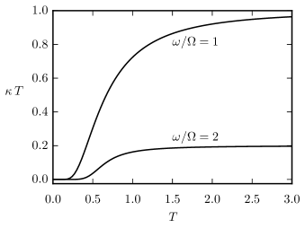
Figure 1: Thermal conductance $\kappa$ times temperature $T$ as a function of $T$ according to the quantum FPK approach, equation (33), for two values of the ratio $\omega/\Omega$. The parameters and constants $g$, $\gamma$, $\Omega$, $\hbar$ and $k_{B}$ are taken to be equal to unity.

To determine the heat flux, we should use equation (9). However, instead of doing so, we use a simpler form, obtained as follows. From equation (20), the evolution equation for $\langle p_{i}^{2}\rangle/2m$ is

$$\frac{1}{2m}\frac{d}{dt}\langle p_{i}^{2}\rangle=-\frac{\omega^{2}}{2}\langle p_{i}x_{i}+x_{i}p_{i}\rangle-\frac{\hbar\varepsilon}{m}\langle p_{i}\sigma_{x}\rangle-\phi_{i}$$ (27)

where $\phi_{i}$ is given by (9). In the stationary state, the left-hand side vanishes, $\langle p_{i}x_{i}+x_{i}p_{i}\rangle=0$, and we are left with the simpler form for the heat flux $\phi=(\hbar\varepsilon/m)\langle p_{1}\sigma_{x}\rangle$. Using $\langle p_{1}\sigma_{x}\rangle$ obtained from the solution of the set of equations (21), (22), (23), (24), and (25), we find

$$\phi=\frac{2g^{2}\gamma\Omega^{2}\hbar\omega\,\psi_{1}\psi_{2}(v_{1}-v_{2})}{(\Gamma_{1}^{2}+\Lambda^{2})\psi_{2}v_{2}+(\Gamma_{2}^{2}+\Lambda^{2})\psi_{1}v_{1}},$$ (28)

where

$$\Gamma_{i}=\gamma\Omega c_{i},$$ (29)

$$v_{i}=\frac{\hbar\Omega}{2}\coth\frac{\beta_{i}\hbar\Omega}{2},$$ (30)

$$\psi_{i}=\frac{\sinh\beta_{i}\hbar\Omega}{\beta_{i}\hbar\Omega}.$$ (31)

We have also used the relation $g=(\hbar/2m\omega)^{1/2}\varepsilon$. From expression (28) we see that the entropy production rate $\Pi$, given by equation (13), is positive. Indeed, if $T_{1}>T_{2}$ then $\beta_{1}<\beta_{2}$ and $v_{1}>v_{2}$ implying $\phi>0$ and $\Pi>0$. The same conclusion follows if $T_{1}<T_{2}$.

It is worth to write down the average $\langle\sigma_{z}\rangle$, which is related to the atomic population $n$ by $n=(1+\langle\sigma_{z}\rangle)/2$. It is given by

$$\langle\sigma_{z}\rangle=-\frac{\hbar\Omega}{2}\frac{(\Gamma_{1}^{2}+\Lambda^{2})\psi_{2}+(\Gamma_{2}^{2}+\Lambda^{2})\psi_{1}}{(\Gamma_{1}^{2}+\Lambda^{2})\psi_{2}v_{2}+(\Gamma_{2}^{2}+\Lambda^{2})\psi_{1}v_{1}},$$ (32)

valid up to linear terms in the couplling $\varepsilon$.

To find the conductance $\kappa$ we start by writing $T_{1}=T+\Delta T/2$ and $T_{2}=T-\Delta T/2$. The conductance is obtained from $\kappa=\phi/\Delta T$ by taking the limit $\Delta T\to 0$, and is given by

$$\kappa=\frac{g^{2}\gamma\Omega^{2}\hbar\omega}{(\gamma^{2}\Omega^{2}c^{2}+\Lambda^{2})T},$$ (33)

where

$$c=\frac{\sinh\beta\hbar\omega}{\beta\hbar\omega}.$$ (34)

When $\Omega\gg\omega$, the regime where the transitions of the two-level atom is decoupled from the oscillators, it turns out that the conductance is suppressed. This can be seen in equation (33) where $\kappa$ vanishes in the limit $\omega/\Omega\to 0$.

When $\Delta T\to 0$, the average $\langle\sigma_{z}\rangle$, given by (32), approaches the value

$$\langle\sigma_{z}\rangle=-\tanh\frac{\beta\hbar\Omega}{2},$$ (35)

which is precisely the result we expect to obtain when the temperatures of the reservoirs are the same, that is, in thermodynamic equilibrium.

It is worth mentioning that in the high temperature limit the conductance reduces to

$$\kappa=\frac{g^{2}\gamma\Omega^{2}\hbar\omega}{(\gamma^{2}\Omega^{2}+\Lambda^{2})T},$$ (36)

because in this limit, $c\to 1$. On the other regime, that is, at low temperatures, we get

$$\kappa=k_{B}\frac{4g^{2}}{\gamma}(\beta\hbar\omega)^{3}e^{-2\beta\hbar\omega},$$ (37)

and $\kappa$ vanishes when $T\to 0$.

The thermal conductance $\kappa$ is shown in figure 1 as a function of temperature. We see that $\kappa T$ approaches a constant when $T\to\infty$, in accordance with expression (36) which shows that, at high temperatures, $\kappa$ is proportional to the inverse of temperature.

III Lindblad Master Equation

III.1 Contact with heat reservoirs

In this approach, the master equation, which gives the time evolution of the density matrix $\rho$, is given by asadian2013 ; breuer2002

$$\frac{d\rho}{dt}=\frac{1}{i\hbar}[{\cal H},\rho]+{\cal D}_{1}(\rho)+{\cal D}_{2}(\rho),$$ (38)

where, here, ${\cal H}$ is given by equation (2), and ${\cal D}_{i}(\rho)$ is the dissipator, which is a sum of Lindblad operators,

$${\cal D}_{i}(\rho)=\gamma(\bar{n}_{i}+1)(a_{i}\rho a_{i}^{\dagger}-\frac{1}{2}a_{i}^{\dagger}a_{i}\rho-\frac{1}{2}\rho a_{i}^{\dagger}a_{i})+\\ +\gamma\bar{n}_{i}(a_{i}^{\dagger}\rho a_{i}-\frac{1}{2}a_{i}a_{i}^{\dagger}\rho-\frac{1}{2}\rho a_{i}a_{i}^{\dagger}),$$ (39)

and

$$\bar{n}_{i}=\frac{1}{e^{\beta_{i}\hbar\omega}-1}$$ (40)

is the Bose-Einstein distribution. We remark that ${\cal D}_{i}$ are local Lindblad dissipators and that equation (39) gives an adequate description of the system only in the regime of weak interactions, which is precisely the regime considered here.

From the Lindblad master equation, one can calculate again the time evolution of the average energy $U=\langle\cal{H}\rangle=\rm{Tr}\{\cal{H}\rho\}$ given by equation $(7)$, where the heat flux $\phi_{i}$ now reads

$$\phi_{i}=-\mathrm{Tr}\left\{\mathcal{D}_{i}\mathcal{H}\right\}.$$ (41)

To find an expression for the entropy production rate we start by postulating that the flux of entropy related to each reservoir is the heat flux divided by its temperature. Therefore the total entropy heat flux is

$$\Phi=\sum_{i}\frac{\phi_{i}}{T_{i}}.$$ (42)

Next we determine the time derivative of the entropy of the system $S=-k_{B}{\rm Tr}\rho\ln\rho$ and use the expression $dS/dt=\Pi-\Phi$ to find the rate of entropy production,

$$\Pi=-k_{B}\sum_{i}{\rm Tr}\{{\cal D}_{i}(\ln\rho+\beta_{i}\mathcal{H})\}.$$ (43)

In the stationary state, $\Pi=\Phi$, and we may use expression (42) to write

$$\Phi=\phi\left(\frac{1}{T_{2}}-\frac{1}{T_{1}}\right),$$ (44)

where $\phi=-\phi_{1}=\phi_{2}$.

When the temperatures are the same, expression (43) reduces to

$$\Pi=-k_{B}\sum_{i}{\rm Tr}\{{\cal D}_{i}(\ln\rho-\ln\rho_{0})\},$$ (45)

where $\rho_{0}=(1/Z)e^{-\beta{\cal H}}$ is the equilibrium Gibbs distribution. Equation (45) gives the usual expression for the rate of entropy production associated to master equation of the Lindblad type breuer2002 .

The establishment of quations (42) and (43) for the heat flux and the entropy production rate requires that the equilibrium solution of the master equation is the Gibbs state $\rho_{0}=(1/Z)e^{-\beta{\cal H}}$, otherwise the entropy production rate will not vanish in equilibrium. This requirement means to say that ${\cal D}_{i}(\rho_{0})$ should vanish when the temperatures are the same. However, the local Lindblad dissipators of the type (39) do not hold this property and should thus be understood as approximations, valid, in the present case, in the regime of weak interactions. The calculations of the heat flux and the entropy flux by equations (41) and (42) should therefore be understood as approximate results, but this is only because the local dissipators (39) are approximations.

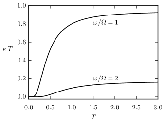
Figure 2: Thermal conductance $\kappa$ times temperature $T$ as a function of $T$ according to the Lindblad master equation approach, equation (57), for two values of the ratio $\omega/\Omega$. The parameters and constants $g$, $\gamma$, $\Omega$, $\hbar$ and $k_{B}$ are taken to be equal to unity.

III.2 Thermal Conductance

From the master equation we can again determine the time evolution of the quantities $\langle a_{i}\sigma_{x}\rangle$, $\langle a_{i}\sigma_{y}\rangle$, $\langle a_{i}^{\dagger}\sigma_{x}\rangle$, $\langle a_{i}^{\dagger}\sigma_{y}\rangle$ and $\langle\sigma_{z}\rangle$. If $\langle A\rangle={\rm Tr}\{A\rho\}$ is one of these quantities, then from the master Lindblad equation we may obtain the following formula for its time evolution

$$\frac{d}{dt}\langle A\rangle=\frac{1}{i\hbar}\langle[A,{\cal H}]\rangle+\sum_{i}{\rm Tr}\{A{\cal D}_{i}\}.$$ (46)

Using these equation and the definition (39) of ${\cal D}_{i}$, we obtained the evolution of the quantities of interest. In the stationary state, these equations give the following set of equations

$$\langle a_{1}\sigma_{y}\rangle+\langle a_{1}^{\dagger}\sigma_{y}\rangle=\langle a_{2}\sigma_{y}\rangle+\langle a_{2}^{\dagger}\sigma_{y}\rangle,$$ (47)

$$\alpha\langle a_{i}\sigma_{x}\rangle+\Omega\langle a_{i}\sigma_{y}\rangle+ig=0,$$ (48)

$$\alpha^{*}\langle a_{i}^{\dagger}\sigma_{x}\rangle+\Omega\langle a_{i}^{\dagger}\sigma_{y}\rangle-ig=0,$$ (49)

$$\alpha\langle a_{i}\sigma_{y}\rangle-\Omega\langle a_{i}\sigma_{x}\rangle+g\left(2\bar{n}+1\right)\langle\sigma_{z}\rangle=0,$$ (50)

$$\alpha^{*}\langle a_{i}^{\dagger}\sigma_{y}\rangle-\Omega\langle a_{i}^{\dagger}\sigma_{x}\rangle+g\left(2\bar{n}+1\right)\langle\sigma_{z}\rangle=0,$$ (51)

where $\alpha=\gamma/2+i\omega$. This is a closed set of nine equations in the variables $\langle\sigma_{z}\rangle$, $\langle a_{1}\sigma_{x}\rangle$, $\langle a_{2}\sigma_{x}\rangle$, $\langle a_{1}\sigma_{y}\rangle$, $\langle a_{2}\sigma_{y}\rangle$, $\langle a_{1}^{\dagger}\sigma_{x}\rangle$, $\langle a_{2}^{\dagger}\sigma_{x}\rangle$, $\langle a_{1}^{\dagger}\sigma_{y}\rangle$, and $\langle a_{2}^{\dagger}\sigma_{y}\rangle$. Notice the last four equation are valid for $i=1,2$. The set of equation is valid for small values of the coupling constant $g$ and is easily solved to get the correlations in closed forms. Notice that, with the exception of the variable $\langle\sigma_{z}\rangle$, all variables are proportional to the coupling constant $g$ whereas $\langle\sigma_{z}\rangle$ does not depend on $g$.

To obtain an expression for the heat flux, we replace the definition of ${\cal D}_{i}$, given by equation (39), into equation (41),

$$\phi_{i}=-\hbar\omega{\rm Tr}\{a_{i}^{\dagger}a_{i}{\cal D}_{i}\}+\frac{\hbar g\gamma}{2}\langle(a_{i}^{\dagger}+a_{i})\sigma_{x}\rangle$$ (52)

Now, the evolution equation for the quantity $\langle a_{i}^{\dagger}a_{i}\rangle$ is

$$\frac{d}{dt}\langle a_{i}^{\dagger}a_{i}\rangle=-ig\langle(a_{i}^{\dagger}-a_{i})\sigma_{x}\rangle+{\rm Tr}\{a_{i}^{\dagger}a_{i}{\cal D}_{i}\}$$ (53)

In the stationary state, the left-hand side vanishes. Summing up these two last equations, we obtain the the heat flux $\phi=-\phi_{1}$ in the form

$$\phi=i\hbar\omega g\langle(a_{1}^{\dagger}-a_{1})\sigma_{x}\rangle-\frac{\hbar g\gamma}{2}\langle(a_{1}^{\dagger}+a_{1})\sigma_{x}\rangle.$$ (54)

From $\langle a_{1}\sigma_{x}\rangle$ and $\langle a_{1}^{\dagger}\sigma_{x}\rangle$, obtained from the stationary solution, we get the heat flux

$$\phi=\frac{32g^{2}\gamma\Omega^{2}\hbar\omega}{\gamma^{4}+8\gamma^{2}(\omega^{2}+\Omega^{2})+16\Lambda^{2}}\frac{\bar{n}_{1}-\bar{n}_{2}}{1+\bar{n}_{1}+\bar{n}_{2}}.$$ (55)

As we did in the previous approach, it is worth to write down the mean atomic population

$$\langle\sigma_{z}\rangle=-\frac{8\omega\Omega}{\gamma^{2}+4(\omega^{2}+\Omega^{2})}\frac{1}{1+\bar{n}_{1}+\bar{n}_{2}}.$$ (56)

By writing again the temperatures as $T_{1}=T+\Delta T/2$ and $T_{2}=T-\Delta T/2$, it is possible to obtain the thermal conductance $\kappa$. In this case it reads

$$\kappa=\frac{16g^{2}\gamma\Omega^{2}\hbar\omega}{\gamma^{4}+8\gamma^{2}(\omega^{2}+\Omega^{2})+16\Lambda^{2}}\frac{1}{cT}.$$ (57)

In this case, the quantity $\langle\sigma_{z}\rangle$ becomes

$$\langle\sigma_{z}\rangle=-\frac{8\omega\Omega}{\gamma^{2}+4\left(\omega^{2}+\Omega^{2}\right)}\tanh\frac{\beta\hbar\omega}{2},$$ (58)

which, as we can see, does not correspond to the correct result for the thermodynamic equilibrium. This incorrect result is to be expected because local phenomenological Lindblad master equations do not lead to proper thermalization, that is, the Gibbs probability distribution $\rho_{0}=(1/Z)e^{-\beta{\cal H}}$ is not the stationary solution of the Lindblad master equation (38).

In the high temperature limit, the thermal conductance reduces to

$$\kappa=\frac{16g^{2}\gamma\Omega^{2}\hbar\omega}{\gamma^{4}+8\gamma^{2}(\omega^{2}+\Omega^{2})+16\Lambda^{2}}\frac{1}{T},$$ (59)

because $c\to 1$ in this limit. At low temperatures, on the other hand, the thermal conductance becomes

$$\kappa=k_{B}\frac{32g^{2}\gamma\Omega^{2}(\beta\hbar\omega)^{2}}{\gamma^{4}+8\gamma^{2}\left(\omega^{2}+\Omega^{2}\right)+16\Lambda^{2}}e^{-\beta\hbar\omega},$$ (60)

and $\kappa$ vanishes when $T\to 0$.

The thermal conductance $\kappa$ is shown in figure 2 as a function of temperature. We see that $\kappa T$ approaches a constant when $T\to\infty$, in accordance with expression (59) which shows that, at high temperatures, $\kappa$ is proportional to the inverse of temperature. In this respect, the two approaches give similar results.

IV Discussion

We have determined the quantum conductance of a system consisting of two level atom coupled to two harmonic oscillators by the use of two distinct methods. These two methods should be understood as two distinct theories about open quantum systems which differ in the way the contact of the system with the heat bath is treated. In the case of the quantum FPK, the contact with a heat bath is advanced in terms of a dissipation-fluctuation approach, described by each term $[x_{i},J_{i}]$ on the summation on the right-hand side of equation (4). In both cases we have set up equations for the correlations which were determined in closed form. From these correlations we have obtained the heat flux and the conductance, which is found to be proportional to coupling constant squared. At high temperature the conductance were found to be proportional to the inverse of temperature, $\kappa\sim T^{-1}$ for both cases. We point out that, at resonance, $\omega=\Omega$, and assuming $\gamma$ much smaller that $\omega$, both approaches yields the same result $\kappa=g^{2}\hbar\omega/\gamma T$. At low temperature the conductance vanishes with temperature as $\kappa\sim e^{-k/T}/T^{n}$ with $n=3$ for the first method and $n=2$ for the second method. All calculations were performed for small values of the coupling constant.

We have also determined the atomic population, $n=(1+\langle\sigma_{z}\rangle)/2$. Up to linear order in the coupling constant, it is finite and, when the difference in the temperatures of the reservoirs vanish, it should be identical to the equilibrium value. Indeed this is what happens when we use the quantum FPK approach, as can be seen in equation (32). However, this is not the case when we use the phenomenological Lindblad master equation with local dissipators (38). In this case, the atomic population $\langle\sigma_{z}\rangle$, given by (58), differs from the equilibrium value.

We have also determined the rate of entropy production for the case of the quantum FPK approach. In this approach, the rate of entropy production, according to reference oliveira2016 , is defined by equation (11). Using this definition, we obtain equation (13), which shows that the rate of entropy production is a product of the heat flux $\phi$ and the thermodynamic force $(T_{2}^{-1}-T_{1}^{-1})$, and proven to be positive as expected. For small values of $\Delta T=T_{1}-T_{2}$, we may write $\Pi=\kappa(\Delta T/T)^{2}$ which is clearly positive because $\kappa$ is positive.

References

- (1) I. I. Rabi, Phys. Rev. 49, 324 (1936); 51, 652 (1937).
- (2) M. O. Scully and M. S. Zubairy, Quantum Optics, Cambridge University Press, Cambridge, 1997.
- (3) J. Larson, Physica Scr. 76, 146 (2007)
- (4) D. Braak, Phys. Rev. Lett. 107, 100401 (2011).
- (5) J. Larson, Phys. Rev. Lett. 108, 033601 (2012).
- (6) L. Yu, S. Zhu, Q. Liang, G. Chen, and S. Jia, Phys. Rev. A 86, 015803 (2012)
- (7) Q. Xie, H. Zhong, M. T. Batchelor, and C. Lee, arXiv: 1609.00434.
- (8) J. M. Raimond, M. Brune, and S. Haroche, Rev. Mod. Phys. 73, 565 (2001).
- (9) T. Holstein, Ann. Phys. 8, 343 (1959).
- (10) S. A. Chilingaryan and B. M. Rodriguez-Lara, J. Phys. B 48, 245501 (2015).
- (11) R. J. Schoelkopf and S. M. Girvin, Nature 451, 664 (2008).
- (12) J. M. Martinis and K. Osborne, arXiv: cond-mat/0402415.
- (13) J. Clarke and F. K. Whilhelm, Nature 453, 1031 (2008).
- (14) M. H. Devoret, A. Wallraff and J. M. Martinis, arXiv: cond-mat/0411174.
- (15) A. Blais, R.-S. Huang, A. Wallraff, S. M. Girvin, and R. J. Schoelkopf, Phys. Rev. A 69, 062320 (2004).
- (16) K. Saito, S. Takesue, and S. Miyashita Phys. Rev. E 54, 2404 (1996)
- (17) A. Asadian, D. Manzano, M. Tiersch, and H. J. Briegel, Phys. Rev. E 87, 012107 (2013).
- (18) T. Tomé and M. J. de Oliveira, Phys. Rev. E 82, 021120 (2010).
- (19) M. J. de Oliveira, Phys. Rev. E 94, 012128 (2016).
- (20) E. Solano-Carrillo and A. J. Mills, Phys. Rev. B 93, 224305 (2016).
- (21) E. Solano-Carrillo, Phys. Rev. E 94, 062116 (2016).
- (22) H.-P. Breuer and F. Petruccione, The Theory of Open Quantum System, Oxford University Press, 2002.