Multi-fidelity Bayesian Optimisation with Continuous Approximations
Abstract
Bandit methods for black-box optimisation, such as Bayesian optimisation, are used in a variety of applications including hyper-parameter tuning and experiment design. Recently, multi-fidelity methods have garnered considerable attention since function evaluations have become increasingly expensive in such applications. Multi-fidelity methods use cheap approximations to the function of interest to speed up the overall optimisation process. However, most multi-fidelity methods assume only a finite number of approximations. In many practical applications however, a continuous spectrum of approximations might be available. For instance, when tuning an expensive neural network, one might choose to approximate the cross validation performance using less data and/or few training iterations . Here, the approximations are best viewed as arising out of a continuous two dimensional space . In this work, we develop a Bayesian optimisation method, BOCA, for this setting. We characterise its theoretical properties and show that it achieves better regret than than strategies which ignore the approximations. BOCA outperforms several other baselines in synthetic and real experiments.
1 Introduction
Many tasks in scientific and engineering applications can be framed as bandit optimisation problems, where we need to sequentially evaluate a noisy black-box function with the goal of finding its optimum. Some applications include hyper-parameter tuning in machine learning (Snoek et al., 2012; Hutter et al., 2011), optimal policy search (Lizotte et al., 2007; Martinez-Cantin et al., 2007) and scientific experiments (Parkinson et al., 2006; Gonzalez et al., 2014). Typically, in such applications, each function evaluation is expensive and historically, the bandit literature has focused on developing methods for finding the optimum while keeping the number of evaluations to at a minimum.
However, with increasingly expensive function evaluations, conventional methods have become infeasible as a significant cost needs to be expended before we can learn anything about . As a result, multi-fidelity optimisation methods have recently gained attention (Kandasamy et al., 2016a; Li et al., 2016; Cutler et al., 2014). As the name suggests, these methods assume that we have access to lower fidelity approximations to which can be evaluated instead of . The lower the fidelity, the cheaper the evaluation, but it provides less accurate information about . For example, when optimising the configuration of an expensive real world robot, its performance can be approximated using cheaper computer simulations. The goal is to use the cheap approximations to guide search for the optimum of , and reduce the overall cost of optimisation. However, most multi-fidelity work assume only a finite number of approximations. In this paper, we study multi-fidelity optimisation when there is access to a continuous spectrum of approximations.
To motivate this, consider tuning a classification algorithm over a space of hyper-parameters by maximising a validation set accuracy. The algorithm is to be trained using data points via an iterative algorithm for iterations. However, we wish to use fewer training points and/or fewer iterations to approximate the validation accuracy. We can view validation accuracy as a function where evaluating requires training the algorithm with points for iterations with the hyper-parameters . If the training complexity of the algorithm is quadratic in data size and linear in the number of iterations, then the cost of this evaluation is . Our goal is to find the optimum when , and , i.e. we wish to maximise .
In this setting, while are technically discrete choices, they are more naturally viewed as coming from a continuous dimensional fidelity space, . One might hope that cheaper queries to with less than can be used to learn about and consequently optimise it using less overall cost. Indeed, this is the case with many machine learning algorithms where cross validation performance tends to vary smoothly with data set size and number of iterations. Therefore, one may use cheap low fidelity experiments with small to discard bad hyper-parameters and deploy expensive high fidelity experiments with large only in a small but promising region. The main theoretical result of this paper (Theorem 1) shows that our proposed algorithm, BOCA, exhibits precisely this behaviour.
Continuous approximations also arise in simulation studies: where simulations can be carried out at varying levels of granularity, on-line advertising: where an ad can be controlled by continuous parameters such as display time or target audience, and several other experiment design tasks. In fact, in many multi-fidelity papers, the finite approximations were obtained by discretising a continuous space (Kandasamy et al., 2016a; Huang et al., 2006). Here, we study a Bayesian Optimisation technique that is directly designed for continuous fidelity spaces and is potentially applicable to more general spaces. Our main contributions are,
-
1.
A novel setting and model for multi-fidelity optimisation with continuous approximations using Gaussian process (GP) assumptions. We develop a novel algorithm, BOCA, for this setting.
-
2.
A theoretical analysis characterising the behaviour and regret bound for BOCA.
-
3.
An empirical study which demonstrates that BOCA outperforms alternatives, both multi-fidelity and otherwise, on a series of synthetic problems and real examples in hyper-parameter tuning and astrophysics.
Related Work
Bayesian optimisation (BO), refers to a suite of techniques for bandit optimisation which use a prior belief distribution for . While there are several techniques for BO (Mockus, 1994; Jones et al., 1998; Thompson, 1933; Hernández-Lobato et al., 2014; de Freitas et al., 2012), our work will build on the Gaussian process upper confidence bound (GP-UCB) algorithm of Srinivas et al. (2010). GP-UCB models as a GP and uses upper confidence bound (UCB) (Auer, 2003) techniques to determine the next point for evaluation.
BO techniques have been used in developing multi-fidelity optimisation methods in various applications such as hyper-parameter tuning and industrial design (Huang et al., 2006; Swersky et al., 2013; Klein et al., 2015; Forrester et al., 2007; Poloczek et al., 2016). However, these methods are either problem specific and/or only use a finite number of fidelities. Further, none of them come with theoretical underpinnings. Recent work has studied multi-fidelity methods for specific problems such as hyper-parameter tuning, active learning and reinforcement learning (Agarwal et al., 2011; Sabharwal et al., 2015; Cutler et al., 2014; Zhang & Chaudhuri, 2015; Li et al., 2016). While some of the above tasks can be framed as optimisation problems, the methods themselves are specific to the problem considered. Our method is more general as it applies to any bandit optimisation task.
Perhaps the closest work to us is that of Kandasamy et al. (2016a, b) who developed MF-GP-UCB assuming a finite number of approximations to . While this line of work was the first to provide theoretical guarantees for multi-fidelity optimisation, it has two important shortcomings. First, they make strong assumptions, particularly a uniform bound on the difference between the expensive function and an approximation. This does not allow for instances where an approximation might be good at certain regions but not at the other. In contrast, our probabilistic treatment between fidelities is is robust to such cases. Second, their model does not allow sharing information between fidelities; each approximation is treated independently. Not only is this wasteful as lower fidelities can provide useful information about higher fidelities, it also means that the algorithm might perform poorly if the fidelities are not designed properly. We demonstrate this with an experiment in Section 4. On the other hand, our model allows sharing information across the fidelity space in a natural way. In addition, we can also handle continuous approximations whereas their method is strictly for a finite number of approximations. That said, BOCA inherits a key intuition from MF-GP-UCB, which is to choose a fidelity only if we have sufficiently reduced the uncertainty at all lower fidelities. Besides this, there are considerable differences in the mechanics of the algorithm and proof techniques. As we proceed, we will draw further comparisons to Kandasamy et al. (2016a).
2 Preliminaries
2.1 Some Background Material
Gaussian processes: A GP over a space is a random process from to . GPs are typically used as a prior for functions in Bayesian nonparametrics. It is characterised by a mean function and a covariance function (or kernel) . If , then is distributed normally for all . Suppose that we are given observations from this GP, where , and . Then the posterior process is also a GP with mean and covariance given by
| (1) | ||||
where is a vector with , and are such that . The matrix is given by . We refer the reader to chapter 2 of Rasmussen & Williams (2006) for more on the basics of GPs and their use in regression.
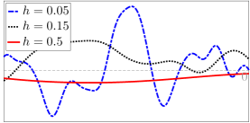
Radial kernels: The prior covariance functions of GPs are typically taken to be radial kernels; some examples are the squared exponential (SE) and Matérn kernels. Using a radial kernel means that the prior covariance can be written as and depends only on the distance between and . Here, the scale parameter captures the magnitude could deviate from . The function is a decreasing function with . In this paper, we will use the SE kernel in a running example to convey the intuitions in our methods. For the SE kernel, , where , called the bandwidth of the kernel, controls the smoothness of the GP. When is large, the samples drawn from the GP tend to be smoother as illustrated in Fig. 1. We will reference this observation frequently in the text.
GP-UCB: The Gaussian Process Upper Confidence Bound (GP-UCB) algorithm of Srinivas et al. (2010) is a method for bandit optimisation, which, like many other BO methods, models as a sample from a Gaussian process. At time , the next point for evaluating is chosen via the following procedure. First, we construct an upper confidence bound for the GP. is the posterior mean of the GP conditioned on the previous evaluations and is the posterior standard deviation. Following other UCB algorithms (Auer, 2003), the next point is chosen by maximising , i.e. . The term encourages an exploitative strategy – in that we want to query regions where we already believe is high – and encourages an exploratory strategy – in that we want to query where we are uncertain about so that we do not miss regions which have not been queried yet. , which is typically increasing with , controls the trade-off between exploration and exploitation. We have provided a brief review of GP-UCB in Appendix A.1.
2.2 Problem Set Up
Our goal in bandit optimisation is to maximise a function , over a domain . When we evaluate at we observe where . Let be a maximiser of and be the maximum value. An algorithm for bandit optimisation is a sequence of points , where at time , the algorithm chooses to evaluate at based on previous queries and observations . After queries to , its goal is to achieve small simple regret , as defined below.
| (2) |
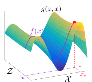
Continuous Approximations: In this work, we will let be a slice of a function that lies in a larger space. Precisely, we will assume the existence of a fidelity space and a function defined on the product space of the fidelity space and domain. The function which we wish to maximise is related to via , where . For instance, in the hyper-parameter tuning example from Section 1, and . Our goal is to find a maximiser . We have illustrated this setup in Fig. 2. In the rest of the manuscript, the term “fidelities” will refer to points in the fidelity space .
The multi-fidelity framework is attractive when the following two conditions are true about the problem.
-
1.
There exist fidelities where evaluating is cheaper than evaluating at . To this end, we will associate a known cost function . In the hyper-parameter tuning example, . It is helpful to think of as being the most expensive fidelity, i.e. maximiser of , and that decreases as we move away from . However, this notion is strictly not necessary for our algorithm or results.
-
2.
The cheap evaluation gives us information about . This is true if is smooth across the fidelity space as illustrated in Fig. 2. As we will describe shortly, this smoothness can be achieved by modelling as a GP with an appropriate kernel for the fidelity space .
In the above setup, a multi-fidelity algorithm is a sequence of query-fidelity pairs where, at time , the algorithm chooses and , and observes where . The choice of can of course depend on the previous fidelity-query-observation triples .
Multi-fidelity Simple Regret: We provide bounds on the simple regret of a multi-fidelity optimisation method after it has spent capital of a resource. Following Srinivas et al. (2010), we will aim to provide any capital bounds, meaning that an algorithm would be expected to do well for all values of (sufficiently large) . Say we have made queries to within capital , i.e. is the random quantity such that . While the cheap evaluations at are useful in guiding search for the optimum of , there is no reward for optimising a cheaper . Accordingly, we define the simple regret after capital as,
This definition reduces to the single fidelity definition (2) when we only query at . It is also similar to the definition in Kandasamy et al. (2016a), but unlike them, we do not impose additional boundedness constraints on or .
Before we proceed, we note that it is customary in the bandit literature to analyse cumulative regret. However, the definition of cumulative regret depends on the application at hand (Kandasamy et al., 2016b) and the results in this paper can be extended to to many sensible notions of cumulative regret. However, both to simplify exposition and since our focus in this paper is optimisation, we stick to simple regret.
Assumptions: As we will be primarily focusing on continuous and compact domains and fidelity spaces, going forward we will assume, without any loss of generality, that and . We discuss non-continuous settings briefly at the end of Section 3. In keeping with similar work in the Bayesian optimisation literature, we will assume and upon querying at we observe where . is the prior covariance defined on the product space. In this work, we will study exclusively of the following form,
| (3) |
Here, is the scale parameter and are radial kernels defined on respectively. The fidelity space kernel is an important component in this work. It controls the smoothness of across the fidelity space and hence determines how much information the lower fidelities provide about . For example, suppose that was a SE kernel. A favourable setting for a multi-fidelity method would be for to have a large bandwidth as that would imply that is very smooth across . We will see that determines the behaviour and theoretical guarantees of BOCA in a natural way when is the SE kernel. To formalise this notion, we will define the following function .
| (4) |
One interpretation of is that it measures the gap in information about when we query at . That is, it is the price we have to pay, in information, for querying at a cheap fidelity. Observe that increases when we move away from in the fidelity space. For the SE kernel, it can be shown111Strictly, , but the inequality is tighter for larger . In any case, is strictly decreasing with . . For large , is smoother across and we can expect the lower fidelities to be more informative about ; as expected the information gap is small for large . If is small and is not smooth, the gap is large and lower fidelities are not as informative.
Before we present our algorithm for the above setup, we will introduce notation for the posterior GPs for and . Let be fidelity, query, observation values from the GP , where was observed when evaluating . We will denote the posterior mean and standard deviation of conditioned on by and respectively ( can be computed from (1) by replacing ). Therefore for all . We will further denote
| (5) |
to be the posterior mean and standard deviation of . It follows that is also a GP and satisfies for all .
3 BOCA: Bayesian Optimisation with Continuous Approximations
BOCA is a sequential strategy to select a domain point and fidelity at time based on previous observations. At time , we will first construct an upper confidence bound for the function we wish to optimise. It takes the form,
| (6) |
Recall from (5) that and are the posterior mean and standard deviation of using the observations from the previous time steps at all fidelities, i.e. the entire space. We will specify in theorems 1, 8. Following other UCB algorithms, our next point in the domain for evaluating is a maximiser of , i.e. .
Next, we need to determine the fidelity to query . For this we will first select a subset of as follows,
| (7) | |||
Here, is the information gap function in (4) and is the posterior standard deviation of , and are the dimensionalities of . The exponent depends on the kernel. For the SE kernel, . We filter out the fidelities we consider at time using three conditions as specified above. We elaborate on these conditions in more detail in Section 3.1. If is not empty, we choose the cheapest fidelity in this set, i.e. . If is empty, we choose .
We have summarised the resulting procedure below in Algorithm 1. An important advantage of BOCA is that it only requires specifying the GP hyper-parameters for such as the kernel . In practice, this can be achieved by various effective heuristics such as maximising the GP marginal likelihood or cross validation which are standard in most BO methods. In contrast, MF-GP-UCB of Kandasamy et al. (2016a) requires tuning several other hyper-parameters.
Input: kernel .
3.1 Fidelity Selection Criterion
We will now provide an intuitive justification for the three conditions in the selection criterion for , i.e., equation (7). Recall that we query only if is empty. The first condition, is fairly obvious; since we wish to optimise and since we are not rewarded for queries at other fidelities, there is no reason to consider fidelities that are more expensive than .
The second condition, says that we will only consider fidelities where the posterior variance is larger than a threshold , which depends critically on two quantities, the cost function and the information gap . As a first step towards parsing this condition, observe that a reasonable multi-fidelity strategy should be inclined to query cheap fidelities and learn about before querying expensive fidelities. Now notice that is monotonically increasing in , therefore, it becomes easier for a cheap to satisfy and be included in at time . Moreover, since we choose to be the minimiser of in , a cheaper fidelity will always be chosen over expensive ones if included in . Second, if a particular fidelity is far away from , it probably contains less information about . Again, a reasonable multi-fidelity strategy should be discouraged from making such queries. This is precisely the role of the information gap which is increasing with . As moves away from , increases and it becomes harder to satisfy . Therefore, such a is less likely to be included in and be considered for evaluation. Our analysis reveals that setting as in (7) is a reasonable trade off between cost and information in the approximations available to us; cheaper fidelities cost less, but provide less accurate information about the function we wish to optimise. It is worth noting that the second condition is similar in spirit to Kandasamy et al. (2016a) who proceed from a lower to higher fidelity only when the lower fidelity variance is smaller than a threshold. However, while they treat the threshold as a hyper-parameter, we are able to explicitly specify theoretically motivated values.
The third condition in (7) is . Since is increasing as we move away from , it says we should exclude fidelities inside a (small) neighbourhood of . Recall that if is empty, BOCA will choose by default. But when it is not empty, we want to prevent situations where we get arbitrarily close to but not actually query at . Such pathologies can occur when we are dealing with a continuum of fidelities and this condition forces BOCA to pick instead of querying very close to it. Observe that since is increasing with , this neighborhood is shrinking with time and therefore the algorithm will eventually have the opportunity to evaluate fidelities close to .
3.2 Theoretical Results
We now present our main theoretical contributions. In order to simplify the exposition and convey the gist of our results, we will only present a simplified version of our theorems. We will suppress constants, terms, and other technical details that arise due to a covering argument in our proofs. A rigorous treatment is available in Appendix B.
Maximum Information Gain: Up until this point, we have not discussed much about the kernel of the domain . Since we are optimising over , it is natural to expect that this will appear in the bounds. Srinivas et al. (2010) showed that the statistical difficulty of GP bandits is determined by the Maximum Information Gain (MIG) which measures the maximum information a subset of observations have about . We denote it by where is a subset of and is the number of queries to . We refer the reader to Appendix B for a formal definition of MIG . For the current exposition however, it suffices to know that depends on the domain kernel , the number of times we have queried , and the volume of the set . The latter dependence on will be most important to us. For instance, when we use an SE kernel for , we have (Seeger et al., 2008). Srinivas et al. (2010) showed that the simple regret for GP-UCB after capital can be bounded by,
| (8) |
where .
In our analysis of BOCA we show that most queries to at fidelity will be confined to a small subset of the domain which contains the optimum . More precisely, after capital , for any , we show that there exists such that the number of queries outside the following set is less than .
| (9) |
Here, is from (4) and is the diameter of . While it is true that any optimisation algorithm would eventually query extensively in a neighbourhood around the optimum, a strong result of the above form is not always possible. For instance, in the case of GP-UCB , the best achievable bound on the number of queries in any set that does not contain is . The fact that the above set exists relies crucially on the multi-fidelity assumptions and the fact that our algorithm leverages information from lower fidelities when querying at . As is small when is smooth across , the set will be small when the approximations are highly informative about . To see this more clearly, consider again the case where is a SE kernel, where we have . When is large and is smooth across , is small as the right side of the inequality is smaller. As BOCA confines most of its evaluations to this small set containing , we will be able to achieve much better regret than GP-UCB. When is small and is not smooth across , the set becomes large and the advantage of multi-fidelity optimisation diminishes.
We now provide an informal statement of our main result below. will denote inequality and equality ignoring constant and terms.
Theorem 1 (Informal, Regret of BOCA).
Let where satisfies (3). Choose . Then, for sufficiently large and for all , there exists depending on such that the following bound holds w.h.p.
In the above bound, the latter term vanishes fast due to the dependence. When comparing this with (8), we see that we outperform GP-UCB by a factor of asymptotically. If is smooth across the fidelity space, is small and the gains over GP-UCB are significant. If becomes less smooth across , the bound decays gracefully, but we are never worse than GP-UCB up to constant factors.
Theorem 1 also has similarities to the bounds of Kandasamy et al. (2016a) who also demonstrate better regret than GP-UCB by showing that it is dominated by queries inside a set which contains the optimum. However, their bounds depend critically on certain threshold hyper-parameters which determine the volume of among other terms in their regret. The authors of that paper note that their bounds will suffer if these hyper-parameters are not chosen appropriately, but do not provide theoretically justified methods to make this choice. In contrast, many of the design choices for BOCA fall out naturally of our modeling assumptions. Beyond this analogue, our results are not comparable to Kandasamy et al. (2016a) as the assumptions are different.
Extensions: While we have focused on continuous due to their wide ranging practical applications, many of the ideas here can be extended to other settings. If is a discrete subset of our work extends straightforwardly. We reiterate that this will not be the same as the finite fidelity MF-GP-UCB algorithm as the assumptions are significantly different. In particular, Kandasamy et al. (2016a) are not able to effectively share information across fidelities as we do. We also believe that Algorithm 1 can be extended to arbitrary fidelity spaces given that a kernel can be defined on . Our results can also be extended to discrete domains and various kernels for by adopting techniques from Srinivas et al. (2010). As with most nonparametric models, BOCA scales poorly with dimension due to the dependence on . For this reason, we also confine our experiments to small . This could be addressed by assuming additional structure on (Djolonga et al., 2013; Kandasamy et al., 2015).
4 Experiments
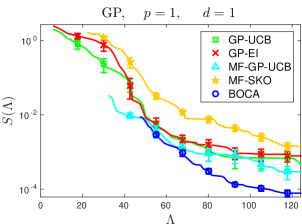
We compare BOCA to the following four baselines: (i) GP-UCB, (ii) the GP-EI criterion in BO (Jones et al., 1998), (iii) MF-GP-UCB (Kandasamy et al., 2016a) and (iv) MF-SKO, the multi-fidelity sequential kriging optimisation method from Huang et al. (2006). All methods are based on GPs and we use the SE kernel for both the fidelity space and domain. The first two are not multi-fidelity methods, while the last two are finite multi-fidelity methods222To our knowledge, the only other work that applies to continuous approximations is Klein et al. (2015) which was developed specifically for hyper-parameter tuning. Further, their implementation is not made available and is not straightforward to implement. . We have described the implementation details for all methods in Appendix C.1.
4.1 Synthetic Experiments
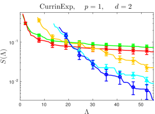
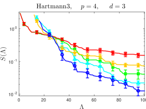
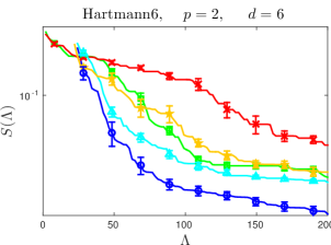
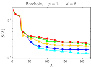
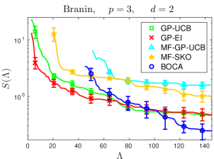
The results for the first set of synthetic experiments are given in Fig. 3. The title of each figure states the function used, and the dimensionalities of the fidelity space and domain. In all cases, the fidelity space was taken to be with being the most expensive fidelity. For MF-GP-UCB and MF-SKO, we used fidelities ( approximations) where the approximations were obtained at and points in the fidelity space. To reflect the setting in our theory, we add Gaussian noise to the function value when observing at any . This makes the problem more challenging than standard global optimisation problems where function evaluations are not noisy. The functions , the cost functions and the noise variances are given in Appendix C.2.
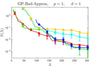
The first two figures in Fig. 3 are simple sanity checks. In both cases, and and the functions were sampled from GPs. The GP was made known to all methods, i.e. the methods used the true GP in picking the next point. In the first figure, we used an SE kernel with bandwidth for and for . The large fidelity bandwidth causes to be smooth across and BOCA outperforms other baselines in this setting. The curve starts mid-way in the figure as BOCA is yet to query at up until that point. The second figure uses the same set up as the first except we used an SE kernel with bandwidth for . Even though is highly unsmooth across , BOCA does not perform poorly. This corroborates a claim that we made earlier that BOCA can naturally adapt to the smoothness of the approximations. The other multi-fidelity methods seem to suffer in this setting.
In the remaining experiments, we use some standard benchmarks for global optimisation. We modify them to obtain and add noise to the observations. As the kernel and other GP hyper-parameters are unknown, we learn them by maximising the marginal likelihood every iterations. This is a common heuristic used in the BO literature. We outperform all methods on all problems except in the case of the Borehole function where MF-GP-UCB does better. The last synthetic experiment is the Branin function given in Fig. 4. We used the same set up as above, but use 10 fidelities for MF-GP-UCB and MF-SKO where the fidelity is obtained at in the fidelity space. Notice that the performance of finite fidelity methods deteriorate. In particular, as MF-GP-UCB does not share information across fidelities, the approximations need to be designed carefully for the algorithm to work well. Our more natural modelling assumptions prevent such pitfalls. We next present two real examples in astrophysics and hyper-parameter tuning. We do not add noise to the observations, but treat it as optimisation tasks, where the goal is to maximise the function.
4.2 Astrophysical Maximum Likelihood Inference
We use data on TypeIa supernova for maximum likelihood inference on cosmological parameters, the Hubble constant , the dark matter fraction and dark energy fraction , hence . The likelihood is given by the Robertson-Walker metric, the computation of which requires a one dimensional numerical integration for each point in the dataset. Unlike typical maximum likelihood problems, here the likelihood is only accessible via point evaluations.
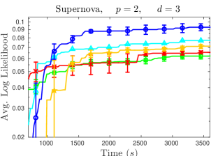
We use the dataset from Davis et al (2007) which has data on supernovae. We construct a dimensional multi-fidelity problem where we can choose between data set size and perform the integration on grids of size via the trapezoidal rule. As the cost function for fidelity selection, we used as the computation time is linear in both parameters. Our goal is to maximise the average log likelihood at . For the finite fidelity methods we use three fidelities with the approximations available at and (which correspond to and after rescaling as in Section 4.1). The results are given in Fig. 4 where we plot the maximum average log likelihood against wall clock time as that is the cost in this experiment. The plot includes the time taken by each method to tune the GPs and determine the next points/fidelities for evaluation.
4.3 Support Vector Classification with news groups
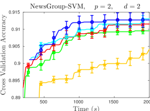
We use the news groups dataset (Joachims, 1996) in a text classification task. We obtain the bag of words representation for each document, convert them to tf-idf features and feed them to a support vector classifier. The goal is to tune the regularisation penalty and the temperature of the rbf kernel both in the range . Hence . The support vector implementation was taken from scikit-learn. We set this up as a dimensional multi-fidelity problem where we can choose a dataset size and the number of training iterations . Each evaluation takes the given dataset of size and splits it up into to perform -fold cross validation. As the cost function for fidelity selection, we used as the training/validation complexity is linear in both parameters. Our goal is to maximise the cross validation accuracy at . For the finite fidelity methods we use three fidelities with the approximations available at and . The results are given in Fig. 4 where we plot the average cross validation accuracy against wall clock time.
5 Conclusion
We studied Bayesian optimisation with continuous approximations, by treating the approximations as arising out of a continuous fidelity space. While previous multi-fidelity literature has predominantly focused on a finite number of approximations, BOCA applies to continuous fidelity spaces and can potentially be extended to arbitrary spaces. We bound the simple regret for BOCA and demonstrate that it is better than methods such as GP-UCB which ignore the approximations and that the gains are determined by the smoothness of the fidelity space. When compared to existing multi-fidelity methods, BOCA is able to share information across fidelities effectively, has more natural modelling assumptions and has fewer hyper-parameters to tune. Empirically, we demonstrate that BOCA is competitive with other baselines in synthetic and real problems.
Going forward, we wish to extend our theoretical results to more general settings. For instance, we believe a stronger bound on the regret might be possible if is a finite dimensional kernel. Since finite dimensional kernels are typically not radial (Sriperumbudur et al., 2016), our analysis techniques will not carry over straightforwardly. Another line of work that we have alluded to is to study more general fidelity spaces with an appropriately defined kernel .
References
- Agarwal et al. (2011) Agarwal, Alekh, Duchi, John C, Bartlett, Peter L, and Levrard, Clement. Oracle inequalities for computationally budgeted model selection. In COLT, 2011.
- Auer (2003) Auer, Peter. Using Confidence Bounds for Exploitation-exploration Trade-offs. J. Mach. Learn. Res., 2003.
- Brochu et al. (2010) Brochu, E., Cora, V. M., and de Freitas, N. A Tutorial on Bayesian Optimization of Expensive Cost Functions, with Application to Active User Modeling and Hierarchical RL. CoRR, 2010.
- Cutler et al. (2014) Cutler, Mark, Walsh, Thomas J., and How, Jonathan P. Reinforcement Learning with Multi-Fidelity Simulators. In ICRA, 2014.
- Davis et al (2007) Davis et al, T. M. Scrutinizing Exotic Cosmological Models Using ESSENCE Supernova Data Combined with Other Cosmological Probes. Astrophysical Journal, 2007.
- de Freitas et al. (2012) de Freitas, Nando, Smola, Alex J., and Zoghi, Masrour. Exponential Regret Bounds for Gaussian Process Bandits with Deterministic Observations. In ICML, 2012.
- Djolonga et al. (2013) Djolonga, J, Krause, A, and Cevher, V. High-Dimensional Gaussian Process Bandits. In NIPS, 2013.
- Forrester et al. (2007) Forrester, Alexander I. J., Sóbester, András, and Keane, Andy J. Multi-fidelity optimization via surrogate modelling. Proceedings of the Royal Society A: Mathematical, Physical and Engineering Science, 2007.
- Ghosal & Roy (2006) Ghosal, Subhashis and Roy, Anindya. Posterior consistency of Gaussian process prior for nonparametric binary regression”. Annals of Statistics, 2006.
- Gonzalez et al. (2014) Gonzalez, J., Longworth, J., James, D., and Lawrence, N. Bayesian Optimization for Synthetic Gene Design. In BayesOpt, 2014.
- Hernández-Lobato et al. (2014) Hernández-Lobato, José Miguel, Hoffman, Matthew W, and Ghahramani, Zoubin. Predictive Entropy Search for Efficient Global Optimization of Black-box Functions. In NIPS, 2014.
- Huang et al. (2006) Huang, D., Allen, T.T., Notz, W.I., and Miller, R.A. Sequential kriging optimization using multiple-fidelity evaluations. Structural and Multidisciplinary Optimization, 2006.
- Hutter et al. (2011) Hutter, Frank, Hoos, Holger H., and Leyton-Brown, Kevin. Sequential Model-based Optimization for General Algorithm Configuration. In LION, 2011.
- Joachims (1996) Joachims, Thorsten. A probabilistic analysis of the rocchio algorithm with tfidf for text categorization. Technical report, DTIC Document, 1996.
- Jones et al. (1993) Jones, D. R., Perttunen, C. D., and Stuckman, B. E. Lipschitzian Optimization Without the Lipschitz Constant. J. Optim. Theory Appl., 1993.
- Jones et al. (1998) Jones, Donald R., Schonlau, Matthias, and Welch, William J. Efficient global optimization of expensive black-box functions. J. of Global Optimization, 1998.
- Kandasamy et al. (2015) Kandasamy, Kirthevasan, Schenider, Jeff, and Póczos, Barnabás. High Dimensional Bayesian Optimisation and Bandits via Additive Models. In International Conference on Machine Learning, 2015.
- Kandasamy et al. (2016a) Kandasamy, Kirthevasan, Dasarathy, Gautam, Oliva, Junier, Schenider, Jeff, and Póczos, Barnabás. Gaussian Process Bandit Optimisation with Multi-fidelity Evaluations. In Advances in Neural Information Processing Systems, 2016a.
- Kandasamy et al. (2016b) Kandasamy, Kirthevasan, Dasarathy, Gautam, Schneider, Jeff, and Poczos, Barnabas. The Multi-fidelity Multi-armed Bandit. In NIPS, 2016b.
- Klein et al. (2015) Klein, A., Bartels, S., Falkner, S., Hennig, P., and Hutter, F. Towards efficient Bayesian Optimization for Big Data. In BayesOpt, 2015.
- Li et al. (2016) Li, Lisha, Jamieson, Kevin, DeSalvo, Giulia, Rostamizadeh, Afshin, and Talwalkar, Ameet. Hyperband: A novel bandit-based approach to hyperparameter optimization. arXiv preprint arXiv:1603.06560, 2016.
- Lizotte et al. (2007) Lizotte, Daniel, Wang, Tao, Bowling, Michael, and Schuurmans, Dale. Automatic gait optimization with gaussian process regression. In IJCAI, 2007.
- Martinez-Cantin et al. (2007) Martinez-Cantin, R., de Freitas, N., Doucet, A., and Castellanos, J. Active Policy Learning for Robot Planning and Exploration under Uncertainty. In Proceedings of Robotics: Science and Systems, 2007.
- Mockus (1994) Mockus, Jonas. Application of Bayesian approach to numerical methods of global and stochastic optimization. Journal of Global Optimization, 1994.
- Parkinson et al. (2006) Parkinson, D., Mukherjee, P., and Liddle, A.. R. A Bayesian model selection analysis of WMAP3. Physical Review, 2006.
- Poloczek et al. (2016) Poloczek, Matthias, Wang, Jialei, and Frazier, Peter I. Multi-information source optimization. arXiv preprint arXiv:1603.00389, 2016.
- Rasmussen & Williams (2006) Rasmussen, C.E. and Williams, C.K.I. Gaussian Processes for Machine Learning. UPG Ltd, 2006.
- Sabharwal et al. (2015) Sabharwal, A, Samulowitz, H, and Tesauro, G. Selecting near-optimal learners via incremental data allocation. In AAAI, 2015.
- Seeger et al. (2008) Seeger, MW., Kakade, SM., and Foster, DP. Information Consistency of Nonparametric Gaussian Process Methods. IEEE Transactions on Information Theory, 2008.
- Snoek et al. (2012) Snoek, J., Larochelle, H., and Adams, R. P. Practical Bayesian Optimization of Machine Learning Algorithms. In NIPS, 2012.
- Srinivas et al. (2010) Srinivas, Niranjan, Krause, Andreas, Kakade, Sham, and Seeger, Matthias. Gaussian Process Optimization in the Bandit Setting: No Regret and Experimental Design. In ICML, 2010.
- Sriperumbudur et al. (2016) Sriperumbudur, Bharath et al. On the optimal estimation of probability measures in weak and strong topologies. Bernoulli, 22(3):1839–1893, 2016.
- Swersky et al. (2013) Swersky, Kevin, Snoek, Jasper, and Adams, Ryan P. Multi-task bayesian optimization. In NIPS, 2013.
- Thompson (1933) Thompson, W. R. On the Likelihood that one Unknown Probability Exceeds Another in View of the Evidence of Two Samples. Biometrika, 1933.
- Xiong et al. (2013) Xiong, Shifeng, Qian, Peter Z. G., and Wu, C. F. Jeff. Sequential design and analysis of high-accuracy and low-accuracy computer codes. Technometrics, 2013.
- Zhang & Chaudhuri (2015) Zhang, C. and Chaudhuri, K. Active Learning from Weak and Strong Labelers. In NIPS, 2015.
Appendix
Appendix A Some Ancillary Material
A.1 Review of GP-UCB
We present a review of the GP-UCB algorithm of Srinivas et al. (2010) which we build on in this work. Here we will assume where is a radial kernel defined on the domain . The algorithm is given below.
Input: kernel .
-
•
, .
-
•
for
-
1.
-
2.
.
-
3.
Perform Bayesian posterior updates to obtain See (1).
-
1.
To present the theoretical results for GP-UCB, we begin by defining the Maximum Information Gain (MIG) which characterises the statistical difficulty of GP bandits.
Definition 2.
(Maximum Information Gain (Srinivas et al., 2010)) Let . Consider any and let be a finite subset. Let such that and . Let . Denote the Shannon Mutual Information by . The Maximum Information Gain of is
Next, we will need the following regularity conditions on the kernel. It is satisfied for four times differentiable kernels such as the SE kernel and Matérn kernel when (Ghosal & Roy, 2006).
Assumption 3.
Let , where is a stationary kernel. The partial derivatives of satisfies the following condition. There exist constants such that,
The following theorem is a bound on the simple regret (2) for GP-UCB.
A.2 Some Technical Results
Here we present some technical lemmas we will need for our analysis.
Lemma 5 (Gaussian Concentration).
Let . Then .
Lemma 6 (Mutual Information in GP, (Srinivas et al., 2010) Lemma 5.3).
Let , and we observe where . Let be a finite subset of and be the function values and observations on this set respectively. Then the Shannon Mutual Information is,
where is the posterior GP variance after observing the first points.
Our next result is a technical lemma taken from Kandasamy et al. (2016a). It will be used in controlling the posterior variance of our and GPs.
Lemma 7 (Posterior Variance Bound (Kandasamy et al., 2016a)).
Let , where and is a radial kernel. Upon evaluating at we observe where . Let and suppose we have observations at and no observations elsewhere. Then the posterior variance (see (1)) at all satisfies,
Proof: The proof is in Section C.0.1 of Kandasamy et al. (2016a) who prove this result as part of a larger proof.
Appendix B Analysis
We will first state a formal version of Theorem 1. Recall from the main text where we stated that most evaluations at are inside the following set .
This is not entirely accurate as it hides a dilation that arises due to a covering argument in our proofs. Precisely, we will show that after queries at any fidelity, BOCA will use most of the evaluations in defined below using .
| (10) |
Here is an ball of radius centred at . is a dilation of by . Notice that for all , as , approaches at a polynomial rate. We now state our main theorem below.
Theorem 8.
In addition to the dilation, Theorem 1 in the main text also suppresses the constants and terms. The next three subsections are devoted to proving the above theorem. In Section B.1 we describe some discretisations for and which we will use in our proofs. Section B.2 gives some lemmas we will need and Section B.3 gives the proof.
B.1 Set Up & Notation
Notation: Let . will denote the number of queries by BOCA at points within time steps. When and , we will overload notation to denote . For , will denote the fidelities which are more expensive than , i.e. .
We will require a fairly delicate set up before we can prove Theorem 8. Let . All sets described in the rest of this subsection are defined with respect to . First define
where recall from (4), is the information gap function. We next define to be an dilation of in the space, i.e.
Finally, we define to be the intersection of with all fidelities satisfying the third condition in (7). That is,
| (11) |
In our proof we will use the second condition in (7) to control the number of queries in .
To control the number of queries outside we first introduce a -covering of the space of size . If , a sufficient covering would be an equally spaced grid having points per side. Let be the points in the covering. to be the points in which are closest to in . Therefore is a partition of .
Now define to be the following function which maps subsets of to subsets of .
| (12) |
That is, maps to fidelities where the information gap is smaller than for all . Next we define , to be the cheapest fidelity in for a subset .
| (13) |
We will see that BOCA will not query inside an at fidelities larger than too many times (see Lemma 12). That is, will be small. We now define as follows,
| (14) |
That is, we first choose ’s that are completely outside and take their cross product with fidelities more expensive than . By design of the above sets, and using the third condition in (7) we can bound the total number of queries as follows,
We will show that the last two terms on the right hand side are small for BOCA and consequently, the first term will be large. But first, we establish a series of technical results which will be useful in proving theorem 8.
B.2 Some Technical Lemmas
The first lemma proves that the UCB in (6) upper bounds on all the domain points chosen for evaluation.
Lemma 9.
Let . Then, with probability , we have
Proof: This is a straightforward argument using Lemma 5 and the union bound. At ,
In the first step we have conditioned w.r.t which allows us to use Lemma 5 as . The statement follows via a union bound over all and the fact that .
Next we show that the GP sample paths are well behaved and that upper bounds on a sufficiently dense subset at each time step. For this we use the following lemma.
Lemma 10.
Let be as given in Theorem 8. Then for all , there exists a discretisation of of size such that the following hold.
-
•
Let be the closest point to in the discretisation. With probability , we have
-
•
With probability , for all and for all , .
Proof: The first part of the proof, which we skip here, uses the regularity condition for in Assumption 3 and mimics the argument in Lemmas 5.6, 5.7 of Srinivas et al. (2010). The second part mimics the proof of Lemma 9 and uses the fact that .
The discretisation in the above lemma is different to the coverings introduced in Section B.1. The next lemma is about the information gap function in (4).
Lemma 11.
Let , and is of the form (3). Suppose we have observations from . Let and . Then implies .
Proof: The proof uses the observation that for radial kernels, the maximum difference between the variances at two points and occurs when all observations are at or vice versa. Now we use and and apply Lemma 7 to obtain . However, As when all observations are at and noting that , we have . Since the above situation characterised the maximum difference between and , this inequality is valid for any general observation set. The proof is completed using the elementary inequality for .
We are now ready to prove Theorem 8. The plan of attack is as follows. We will analyse BOCA after time steps and bound the number of plays at fidelities and outside at . Then we will show that for sufficiently large , the number of random plays is bounded by with high probability. Finally we usee techniques from Srinivas et al. (2010), specifically the maximum information gain, to control the simple regret. However, unlike them we will obtain a tighter bound as we can control the regret due to the sets and separately.
B.3 Proof of Theorem 8
Let be given. We invoke the sets in equations (10), (11), (14) for the given . The following lemma establishes that for any , we will not query inside at fidelities larger than (13) too many times. The proof is given in Section B.3.1.
Lemma 12.
Let which does not contain the optimum. Let be as given in Theorem 8. Then for all , we have
To bound , we will apply Lemma 12 with on all satisfying . Since , does not contain the optimum. As is the union of such sets (14), we have for all (larger than a constant),
Now applying the union bound over all , we get .
Now we will bound the number of plays in using the second condition in (7). We begin with the following Lemma. The proof mimics the argument in Lemma 11 of Kandasamy et al. (2016a) who prove a similar result for GPs defined on just the domain, i.e. where .
Lemma 13.
Let and the diameter of in be and that in be . Suppose we have evaluations of of which are in . Then for any , the posterior variance satisfies,
Let where . If the maximum posterior variance in a certain region is smaller than , then we will not query within that region by the second condition in (7). Further by the third condition, since we will only query at fidelities satisfying , it is sufficient to show that the posterior variance is bounded by at time to prove that we will not query again in that region. For this we can construct a covering of such that . For any , the covering number, which we denote of this construction will typically be polylogarithmic in (See Remark 15 below). Now if there are queries inside a ball in this covering, the posterior variance, by Lemma 13 will be smaller than . Therefore, we will not query any further inside this ball. Hence, the total number of queries in is for appropriate constants . (Also see Remark 16).
Next, we will argue that the number of queries for sufficiently large , is bounded by where, recall . This simply follows from the bounds we have for and .
Since the right hand side is sub-linear in , we can find such that for all , is larger than the right hand side. Therefore for all , . Since our bounds hold with probability for all we can invert the above inequality to bound , the random number of queries after capital . We have . We only need to make sure that which can be guaranteed if .
The final step of the proof is to bound the simple regret after time steps in BOCA. This uses techniques that are now standard in GP bandit optimisation, so we only provide an outline. We begin with the following Lemma.
Lemma 14.
Assume that we have queried at points, of which points are in for any . Let denote the posterior variance of at time , i.e. after queries. Then, . Here is the MIG of after queries to as given in Definition 2.
We now define the quantity below. Readers familiar with the GP bandit literature might see that it is similar to the notion of cumulative regret, but we only consider queries at .
| (15) |
For any we can use Lemmas 9, 10, and 14 and the Cauchy Schwartz inequality to obtain,
For the first term in (15), we use the trivial bound . For the second term we use the fact that and hence, . Noting that , we have . Now, using the fact that for large enough we have,
The theorem now follows from the fact that by definition and that . The failure instances arise out of Lemmas 9, 10 and the bound on , the summation of whose probabilities are bounded by .
Remark 15 (Construction of covering for the SE kernel).
We demonstrate that such a construction is always possible using the SE kernel. Using the inequality for we have,
where will be the diameters of the balls in the covering. Now let and choose
via which we have as stated in the proof. Noting that , using standard results on covering numbers, we can show that the size of this covering will be . A similar argument is possible for Matérn kernels, but the exponent on will be worse.
Remark 16 (Choice of for SE kernel).
From the arguments in our proof and Remark 15, we have that the number of plays in a set is . However, we chose to work work mostly to simplify the proof. It is not hard to see that for and if for all , then . As the capital spent in this region is , by picking we ensure that the capital expended for a certain at all fidelities is roughly the same, i.e. for any , the capital density in fidelities such that will be roughly the same. Kandasamy et al. (2016b) showed that doing so achieved a nearly minimax optimal strategy for cumulative regret in -armed bandits. While it is not clear that this is the best strategy for optimisation under GP assumptions, it did reasonably well in our experiments. We leave it to future work to resolve this.
B.3.1 Proof of Lemma 12
For brevity, we will denote . We will invoke the discretisation used in Lemma 10 via which we have for all . Let be the maximiser of the upper confidence bound in at time . Now note that, . We therefore have,
| (16) |
We now note that
The first step uses Lemma 11. The second step uses the fact that and the last step uses the definition of in (12) whereby we have . Now we plugging this back into (16), we can bound each term in the summation by,
| (17) |
In the first step we have used the following facts, and to conclude,
The second step of (17) uses Lemma 5, the third step uses the conditions on as given in theorem 8 and the last step uses the fact that . Now plug (17) back into (16). The result follows by bounding the sum by an integral and noting that and .
B.3.2 Proof of Lemma 14
Let be the queries in in the order they were queried. Now, assuming that we have queried only inside , denote by , the posterior standard deviation after such queries. Then,
Queries outside will only decrease the variance of the GP so we can upper bound the first sum by the posterior variances of the GP with only the queries in . The third step uses the inequality . The result follows from the fact that maximises the mutual information among all subsets of size .
Appendix C Addendum to Experiments
C.1 Implementation Details
We describe some of our implementation details below.
-
Domain and Fidelity space: Given a problem with arbitrary domain and , we mapped them to and by appropriately linear transforming the coordinates.
-
Initialisation: Following recommendations in Brochu et al. (2010) all GP methods were initialised with uniform random queries with capital, where is the total capital used in the experiment. For GP-UCB and GP-EI all queries were initialised at whereas for the multi-fidelity methods, the fidelities were picked at random from the available fidelities.
-
GP Hyper-parameters: Except in the first two experiments of Fig. 3, the GP hyper-parameters were learned after initialisation by maximising the GP marginal likelihood (Rasmussen & Williams, 2006) and then updated every 25 iterations. We use an SE kernel for both and and instead of using one bandwidth for the entire fidelity space and domain, we learn a bandwidth for each dimension separately. We learn the kernel scale, bandwidths and noise variance using marginal likelihood. The mean of the GP is set to be the median of the observations.
-
Choice of : , as specified in Theorem 8 has unknown constants and tends to be too conservative in practice (Srinivas et al., 2010). Following the recommendations in Kandasamy et al. (2015) we set it to be of the correct “order”; precisely, . Here, is the effective diameter of and is computed by scaling each dimension by the inverse of the bandwidth of the SE kernel for that dimension.
-
Maximising : We used the DiRect algorithm (Jones et al., 1993).
-
Fidelity selection: Since we only worked in low dimensional fidelity spaces, the set was constructed in practice by obtaining a finely sampled grid of and then filtering out those which satisfied the conditions in (7). In the second condition of (7), the threshold can be multiplied up to a constant factor, i.e without affecting our theoretical results. In practice, we started with but we updated it every 20 iterations via the following rule: if the algorithm has queried more than of the time in the last iterations, we decrease it to and if it queried less than of the time we increase it to . But the value is always clipped inbetween and . In practice we observed that the value for usually stabilised around and although in some experiments it shot up to . Changing this way resulted in slightly better performance in practice.
C.2 Description of Synthetic Functions
The following are the synthetic functions used in the paper.
-
GP Samples: For the GP samples in the first two experiments of Figure 3 we used an SE kernel with bandwidth for . For we used bandwidths and for the first and second experiments respectively. The function was constructed by obtaining the GP function values on a grid in the two dimensional space and then interpolating for evaluations in between via bivariate splines. For both experiments we used and the cost function .
-
Currin exponential function: The domain is the two dimensional unit cube and the fidelity was with . We used , and,
-
Hartmann functions: We used . Here are given below for the and dimensional cases and . Then was set as if for . We constructed the and Hartmann functions for the and dimensional cases respectively this way. When , this reduces to the usual Hartmann function commonly used as a benchmark in global optimisation.
For the dimensional case we used , and,
For the dimensional case we used , and,
-
Borehole function: This function was taken from (Xiong et al., 2013). We first let,
Then we define . The domain of the function is and with . We used for the cost function and for the noise variance.
-
Branin function: We use the following function where and .
where , , , and . At , this becomes the standard Branin function used as a benchmark in global optimisation. We used for the cost function and for the noise variance.