The Ratio of the Core to the Extended Emissions
in the Comoving Frame for Blazars

Abstract

In a two-component jet model, the emissions are the sum of the core and extended emissions: $S^{\rm ob}=S_{\rm core}^{\rm ob}+S_{\rm ext}^{\rm ob}$, with the core emissions, $S_{\rm core}^{\rm ob}=fS_{\rm ext}^{\rm ob}\delta^{q}$, being a function of the Doppler factor, $\delta$, the extended emission, $S_{\rm ext}^{\rm ob}$, jet type dependent factor, $q$, and the ratio of the core to the extended emissions in the comoving frame, $f$. The $f$ is an unobservable but important parameter. Following our previous work, we collect 65 blazars with available Doppler factor, $\delta$, superluminal velocity, $\beta_{app}$, and core-dominance parameter, $R$, calculate the ratio, $f$, and peform statistical analyses. We find that the ratio, $f$, in BL Lacs is on average larger than that in FSRQs. We suggest that the difference of the ratio $f$ between FSRQs and BL Lacs is one of the possible reasons that cause the difference of other observed properties between them. We also find some significant correlations between $\log f$ and other parameters, including intrinsic (de-beamed) peak frequency, $\log\nu_{\rm p}^{\rm in}$, intrinsic polarization, $\log P^{\rm in}$, and core-dominance parameter, $\log R$, for the whole sample. In addition, we show that the ratio, $f$, can be estimated by $R$.

fjh@gzhu.edu.cn

12.3456/s78910-011-012-3 #### 123 2016 23–25 25

1 Introduction

Blazars are a particular subclass of the radio-loud active galactic nuclei (AGNs), which have high and variable polarization, large and rapid variation, high energetic $\gamma$-ray emissions, and superluminal motions, etc. Blazars can be divided into two subclassses, namely, flat spectrum radio quasars (FSRQs) and BL Lacertae objects (BL Lacs). The main difference between these two subclasses is that BL Lacs show no (or very weak) emission line features while FSRQs display strong emission lines. However, BL Lacs and FSRQs are quite similar in their continuum emission properties (Fan 2003; Fan & Lin 2003; Fan et al. 2009, 2014; Gupta et al. 2009, 2016; Lin & Fan 2016; Pei et al. 2016; Lin et al. 2017 ).

Following Abdo et al. (2010), blazars can be divided into low synchrotron peaked (LSP, $\nu_{\rm{p}}^{s}<10^{14}$ Hz), intermediate synchrotron peaked (ISP, $10^{14}$ Hz $<\nu_{\rm{p}}^{s}<10^{15}$ Hz), and high synchrotron peaked (HSP, $\nu_{\rm{p}}^{s}>10^{15}$ Hz) sources, from their spectral energy distributions (SEDs) (also see Ackermann et al. 2015; Fan et al. 2015). In our recent work (Fan et al. 2016), the SEDs of 1392 blazars are fitted and the corresponding ${\log\nu^{s}_{p}}$ are obtained, and we classified the 999 Fermi blazars with available redshifts into LSP ($\nu_{\rm{p}}^{s}<10^{14}$ Hz), ISP ($10^{14}$ Hz $<\nu_{\rm{p}}^{s}<10^{15.3}$ Hz), HSP ($\nu_{\rm{p}}^{s}>10^{15.3}$ Hz) .

The extreme observational properties of blazars are attributed to a beaming effect. In a beaming model, the emissions can be separated into the jet and extended components in the comoving frame: $S^{\rm in}=S^{\rm in}_{j}+S^{\rm in}_{ext}=(f+1)S^{\rm in}_{ext}$, where $f=S^{\rm in}_{j}/S^{\rm in}_{ext}$ is the ratio of the intrinsic (de-beamed) jet to the extended emissions. Since the jet emissions are beamed in the observed frame $S^{\rm ob}_{j}=S^{\rm in}_{j}\delta^{q}$, the observed emissions can be expressed in a form: $S^{\rm ob}=(f\delta^{q}+1)S^{\rm ob}_{ext}$, where $\delta=[\Gamma(1-\beta\cos\theta)]^{-1}$ is a Doppler factor, $q$ is a jet type depended parameter: $q=2+\alpha$ for continuous jet, $q=3+\alpha$ for a jet with distinct “blobs” (Lind & Blandford 1985), $\alpha$ is a spectral index, $S_{\nu}\propto\nu^{-\alpha}$, $\theta$ is the viewing angle, $\beta$ is the jet speed in unit of the speed of light, and $\Gamma=1/(1-\beta^{2})^{1/2}$ is the bulk Lorentz factor. In a two-component jet model, the beamed emissions correspond to the core emissions, $S_{\rm core}$, while the unbeamed ones are linked to the extended emissions, $S_{\rm ext}$. Then a core-dominance parameter, $R$, can be defined as

$$R=S^{\rm ob}_{\rm core}/S^{\rm ob}_{\rm ext}=f\delta^{q}.$$ (1)

When the viewing angle, $\theta$, is large, the emission from the receding jet is no longer negligible, then Eq. (1) is replaced by (Orr & Brown 1982, see also Urry & Padovani 1995)

$$R(\theta)=f\{[\Gamma(1-\beta cos\theta)]^{-q}+[\Gamma(1+\beta cos\theta)]^{-q}\}$$ (2)

At a viewing angle of 90 degree, the relation between ratio $f$ and $R_{T}$ is given by

$$R_{T}=R(90^{\circ})=2f/\Gamma^{q}.$$ (3)

Facing the differences and similarities between BL Lacs and FSRQs, some authors suggested that there is an evolution tendency between BL Lacs and FSRQs (e.g., Sambruna et al. 1996). However, no significant difference of black hole mass was found between them in Wu et al. (2002). In 2003, we compiled 41 sources (10 BL Lacs, 27 FSRQs, 4 radio galaxies) with available superluminal velocity, Doppler factor from Lähteenimäki & Valtaoja (1999, hereafter LV99) and core dominance parameter, calculated the ratio, $f$, found the $f$ values in BL Lacs are larger than that in FSRQs, and proposed that the difference in emission line feature between BL Lacs and FSRQs is from their difference in ratio, $f$ (Fan 2003).

Following our previous work (Fan 2003), we compile 65 blazars (with 28 new sources) in order to calculate the ratio, $f$, and then do some statistical analysis. This work is arranged as follows: we will describe the sample and the results in section 2, and give some discussions and conclusions in section 3.

2 Sample and Results

From Eq. (2), we can obtain the ratio (Fan 2003)

$$f=R(\theta)/\{[\Gamma(1-\beta cos\theta)]^{-q}+[\Gamma(1+\beta cos\theta)]^{-q}\}$$ (4)

Although $\Gamma$ and $\theta$ are unobservable parameters, they can be obtained if the Doppler factor, $\delta$, and apparent velocity, $\beta_{app}$ are known, as

$$\Gamma=(\beta_{app}^{2}+\delta^{2}+1)/2\delta,$$ (5)

$$\tan\theta=2\beta_{app}/(\beta_{app}^{2}+\delta^{2}-1),$$ (6)

Thus, from Eq. (4), $f$ can be obtained for a superluminal jet with available apparent velocity, $\beta_{app}$, Doppler factor, $\delta$, and core-dominance parameter, $R(\theta)$.

In a two-component model, we assumed that the polarized emissions are only from the jet and the extended emissions are not polarized. In this case, we assumed that the polarized and unpolarized emissions are proportional to each other (Fan et al. 1997), namely $S_{j}=S_{jp}+S_{jup}=(1+\eta)S_{jup}$, where $\eta=S_{jp}/S_{jup}$. Then, the frequency and polarization at the observers’ frame can be expressed as (e.g., Fan et al. 1997, 2006; Fan 2002),

$$\nu^{\rm ob}=\delta\nu^{\rm in}/(1+z)$$ (7)

$$P^{\rm ob}=\frac{(1+f)\delta^{q}}{1+f\delta^{q}}P^{\rm in}$$ (8)

where $z$ is a redshift, $\nu^{\rm in}$ is an intrinsic frequency, $P^{\rm in}$ is an intrinsic total polarization, which defined as

$$P^{\rm in}=\frac{f}{1+f}P_{j}^{\rm in}=\frac{f}{1+f}\frac{\eta}{1+\eta}$$ (9)

where $P_{j}^{\rm in}$ is the intrinsic jet polarization. Therefore, when $f$ is obtained and $P^{\rm ob}$ is known, $P^{\rm in}$ can be obtained by Eq. (8), and then $\eta$ can be obtained from $P^{\rm in}$ and $f$.

2.1 Sample

In this work, we compile a sample of 65 blazars (18 BL Lacs, 47 FSRQs). They are listed in Table 1, in which, Col. (1) gives IAU name, Col. (2) other name, Col. (3) redshift, Col. (4) classification, “Q” stands for FSRQs and “B” for BL Lacs, Col. (5) apparent speed in units of speed of light, Col. (6) Doppler boosting factor, Col. (7) references of Col. (5) and (6), Cols. (8) and (9) core-dominance parameter and the corresponding references, Col. (10) synchrotron peak frequency ${\log\nu^{\rm s}_{\rm p}}$ from Fan et al. (2016). For the sources with no available ${\log\nu^{s}_{p}}$ in Fan et al. (2016), we use the empirical relationship introduced in Fan et al. (2016) to estimate it, as follow

$${\rm log}\nu_{p}^{s}=\begin{cases}\,\,16+4.238X\,\,\,\,\,\,\,X<0\\ \,\,16+4.005Y\,\,\,\,\,\,\,X>0,\end{cases}$$ (10)

where $X=1-1.262\alpha_{\rm RO}-0.623\alpha_{\rm OX}$, and $Y=1.0+0.034\alpha_{\rm RO}-0.978\alpha_{\rm OX}$, $\alpha_{\rm RO}$ and $\alpha_{\rm OX}$ are the radio-to-optical and optical-to-X-ray effective spectral indexes. The corresponding effective spectral indexes are from BZCAT catalog (Massaro et al. 2015), they are labeled with a “$\ast$”, Cols. (11) and (12) give the optical polarization and the corresponding references.

2.2 Result

2.2.1 Averaged Result

Based on the data listed in Table 1, we calculate the Lorentz factor, $\Gamma$, the viewing angle, $\theta$, the jet speed, $\beta$, the ratio, $f$, the core-dominance parameter at 90 degree, $R_{T}$, the intrinsic peak frequency, $\nu_{\rm p}^{\rm in}$, the intrinsic polarization, $P^{\rm in}$, and the ratio, $\eta$ for the 65 blazars. Those calculated values are listed in Table 2. The corresponding range and averaged values of $\delta$, $\beta_{app}$, $\log R$, $\log\nu_{\rm p}^{\rm s}$, $\log P^{\rm ob}$, $\Gamma$, $\theta$, $\beta$, $\log f$, $\log R_{T}$, $\log\nu_{\rm p}^{\rm in}$ $\log P^{\rm in}$ and $\eta$ are listed in Table 3 for the whole sample, and for BL Lacs and FSRQs separately.

From Table 3, we have that $\log f$ is in a range of $-3.11$ to 0.98, with a averaged value of $<\log f>=-1.06\pm 0.93$ for the case of $q=2+\alpha$, and in a range of $-4.65$ to 0.22, with $<\log f>=-2.09\pm 1.15$ for $q=3+\alpha$ for the whole sample. When the subclasses are considered, we have $<\log f>=-0.40\pm 0.88$ $(q=2+\alpha)$ and $<\log f>=-1.17\pm 0.99$ $(q=3+\alpha)$ for BL Lacs, $<\log f>=-1.31\pm 0.84$ $(q=2+\alpha)$ and $<\log f>=-2.45\pm 1.01$ $(q=3+\alpha)$ for FSRQs. One sample Kolmogorov-Smirnov (K-S) test indicates that the ratio, $f$, follows a lognormal distribution with significant levels being $p=99.7\%$ ($q=2+\alpha$) and $p=55.5\%$ ($q=3+\alpha$) for BL Lacs; $p=25.6\%$ ($q=2+\alpha$) and $p=40.3\%$ ($q=3+\alpha$) for FSRQs. Moreover, for the ratio, $\log f$, K-S test gives that the probability for BL Lacs and FSRQs distributions to be from the same distribution is $1.86\times 10^{-3}$ for $q=2+\alpha$ and $2.20\times 10^{-4}$ for $q=3+\alpha$. From a T-test, the probability that BL Lacs and FSRQs have the same averaged value of $\log f$ is $2.87\times 10^{-4}$ for $q=2+\alpha$, and $2.20\times 10^{-5}$ for $q=3+\alpha$, and the averaged difference in $\log f$ between them is $\Delta(\log f)=0.90\pm 0.24$ for $q=2+\alpha$, and $\Delta(\log f)=1.28\pm 0.28$ for $q=3+\alpha$. Therefore, the distribution and the averaged value of $\log f$ in BL Lacs are different from those in FSRQs, see also Fig. 1.

Some researches (eg., Abdo et al. 2010, Fan et al. 2016) found that peak frequency in BL Lacs are different with that in FSRQs. In this work, we investigate the difference between them in $\log\nu_{\rm p}^{\rm in}$ parameter, and find that $\log\nu_{\rm p}^{\rm in}$ is in a range of 11.07 to 14.62, with an averaged value of $<\log\nu_{\rm p}^{\rm in}>=12.69\pm 0.77$ for the whole sample. Considering the subclasses, we have that $\log\nu_{\rm p}^{\rm s}$ is 12.04 to 14.62 with $<\log\nu_{\rm p}^{\rm in}>=13.11\pm 0.83$ for BL Lacs, $\log\nu_{\rm p}^{\rm in}$ is 11.07 to 13.97 with $<\log\nu_{\rm p}^{\rm in}>=12.52\pm 0.69$ for FSRQs. And the probability (K-S test) for BL Lacs and FSRQs distributions to be from the same distribution is $3.62\%$ in $\log\nu_{\rm p}^{\rm in}$. Thus, BL Lacs show not only larger ratio, $f$, but also higher intrinsic peak frequency than FSRQs.

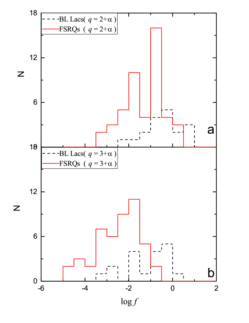
Figure 1: The distribution of the ratio, $\log f$, for the case of $q=2+\alpha$ (a) and $q=3+\alpha$ (b), solid lines are FSRQs and broken lines are BL Lacs.

2.2.2 Correlations

We investigate the correlations between $\log f$ and several parameters (including $\log\nu^{\rm s}_{\rm p}$, $\log\nu_{\rm p}^{\rm in}$, $\log P^{\rm ob}$, $\log P^{\rm in}$, and $\log R$) for the whole sample, as well as the subclasses. The linear regression method is adopted to the correlation analysis, then the corresponding results are listed in Table 4 and shown in Figs. 2–6.

$f$ vs $\nu_{\rm p}^{\rm s}$: Correlations are found between $\log f$ and $\log\nu_{\rm p}^{\rm s}$ for the whole sample with a correlation coefficient $r=0.26$ and a chance probability $p=3.63\%$ for the case of $q=2+\alpha$, see Fig. 2. There are also correlations between $\log f$ and $\log\nu_{\rm p}^{\rm in}$ with $r=0.37$ ($p=2.50\times 10^{-3}$) for the whole sample, and $r=0.37$ ($p=1.13\%$) for FSRQs for $q=2+\alpha$, but no correlation is found for BL Lacs with $r=0.03$ ($p=90.01\%$) for $q=2+\alpha$, see Fig. 3. Some similar results are found in the case of $q=3+\alpha$, see Table 4.

Figure 2: Plot of the ratio, $f$, against the peak frequency for the case of $q=2+\alpha$ (a) and $q=3+\alpha$ (b), the circle symbols stand for BL Lacs and the triangle symbol stand for FSRQs.

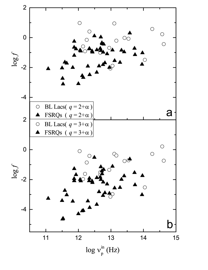
Figure 3: Plot of the ratio, $f$, against the intrinsic peak frequency for the case of $q=2+\alpha$ (a) and $q=3+\alpha$ (b), the circle symbols stand for BL Lacs and the triangle symbol stand for FSRQs.

$f$ vs $P$: The correlations between $\log f$ and $\log P^{\rm ob}$ and between $\log f$ and $\log P^{\rm in}$ are also investigated. No correlation is found between $\log f$ and $\log P^{\rm ob}$ for the whole sample, BL Lacs or FSRQs respectively with chance probabilities being 10.02%, 97.35% and 73.01%. However, strong correlations are found between $\log f$ and $\log P^{\rm in}$ for the whole sample, BL Lacs, and FSRQs, with $r=0.84$ ($p=6.21\times 10^{-16}$), $0.74$ ($7.55\times 10^{-4}$), and $0.82$ ($1.48\times 10^{-10}$) for $q=2+\alpha$ respectively. The corresponding figures are shown in Figs. 4 and 5. Even stronger correlations (see Fig. 5 and Table 4) are seen for $p=3+\alpha$.

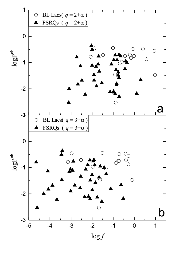
Figure 4: Plot of the observed polarization against the ratio, $f$, for the case of $q=2+\alpha$ (a) and $q=3+\alpha$ (b), the circle symbols stand for BL Lacs and the triangle symbol stand for FSRQs.

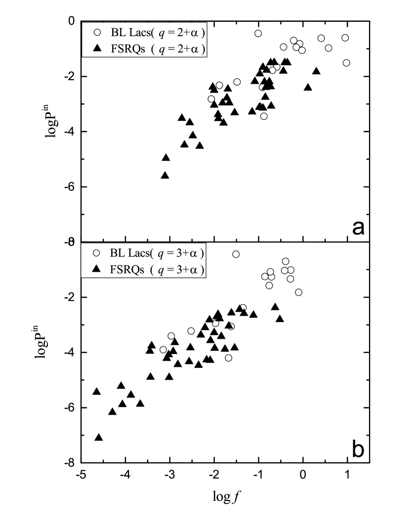
Figure 5: Plot of the intrinsic polarization against the ratio, $f$, for the case of $q=2+\alpha$ (a) and $q=3+\alpha$ (b), the circle symbols stand for BL Lacs and the triangle symbol stand for FSRQs.

$f$ vs $R$: We find significant correlations between $\log f$ and $\log R$ with $r=0.72$ ($p=1.57\times 10^{-11}$) for the whole sample, $r=0.77$ ($p=2.19\times 10^{-4}$) for BL Lacs, and $r=0.77$ ($p=3.13\times 10^{-10}$) for FSRQs for $q=2+\alpha$. Some similar results are found in the case of $q=3+\alpha$, see Table 4. The corresponding figures are shown in Fig. 6. Those results indicate that the ratio, $f$, is directly correlated with a core-dominance parameter ($f\sim R^{0.8}$) regardless of different beaming boosting factors and viewing angles of different sources. The significant correlation between $\log f$ and $\log R$ indicates that the unobservable ratio, $f$, can be estimated from the core-dominance parameter, $R$, namely $\log f=(0.83\pm 0.10)\log R-(1.90\pm 0.13)$ for $q=2+\alpha$ and $\log f=(0.74\pm 0.15)\log R-(2.85\pm 0.20)$ for $q=3+\alpha$, see Table 4 and Fig. 6.

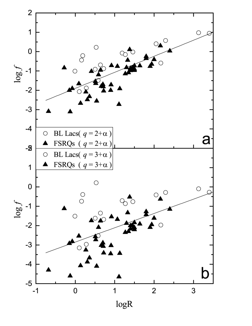
Figure 6: Plot of the core-dominance parameter against the ratio, $f$, for the case of $q=2+\alpha$ (a) and $q=3+\alpha$ (b), the circle symbols stand for BL Lacs and the triangle symbol stand for FSRQs.

3 Discussions and Conclusions

A relativistic beaming model is proposed to explain extreme observational properties for blazars. Some authors (eg., Blandford & Königl 1979; Antonucci & Ulvestad 1985) proposed that the difference of emission line feature between FSRQs and BL Lacs is due to beaming effect. As discussed in our previous work (Fan 2003), if the weak emission line means that the Doppler-boosted emissions dominate the isotropic line emissions, BL Lacs, which have weak emission lines, should have stronger beaming effect than FSRQs. However, the extreme observational properties of FSRQs indicate that the beaming effect of FSRQs is stronger than that of BL Lacs. Others (eg., Padovani 1992, Urry & Padovani 1995) proposed an evolution tendency between FSRQs and BL Lacs, with strong emission line FSRQs evolving into weak line BL Lacs. However there is no difference in black hole masses between FSRQs and BL Lacs in Wu et al. (2002) and our previous work (Fan 2005). So it is very difficult to explain the emission line properties of blazars in that way. Based on all those observational properties, we proposed that a good method should explain both the differences and similarities between FSRQs and BL Lacs, and the ratio, $f$, played an important role on the emission line feature of blazars (Fan 2003).

3.1 Averaged Values

In the present work, we have $<\log f>=-1.06\pm 0.93$ ($q=2+\alpha$), and $<\log f>=-2.09\pm 1.15$ ($q=3+\alpha$) for the whole sample. Some authors suggest that the possible value of the ratio, $f$, is from 0.001 to 1.0 (Padovani & Urry 1990, 1991; Urry et al. 1991; Urry & Padovani 1995; Fan et al. 1997). Our present results ($\log f=-3.11$ to 0.98 for $q=2+\alpha$ and $\log f=-4.65$ to 0.22 for $q=3+\alpha$) are not in conflict with theirs ($\log f=-3$ to 0), but our sample shows a somewhat wider range.

In Fan (2003), we found $<\log f>=-0.99\pm 0.22$ for the whole 41 blazars, $<\log f>=0.11\pm 0.49$ for BL Lacs, and $<\log f>=-1.59\pm 0.19$ for FSRQs for the case of $q=3+\alpha$. A K-S test shows that the probability for the $f$ distributions of BL Lacs and FSRQs to be from the same one is $3\times 10^{-3}$. And the difference between them is $\Delta(\log f)=1.68\pm 0.52$. In this work, $\Delta(\log f)=0.90\pm 0.24$ for $q=2+\alpha$, and $\Delta(\log f)=1.28\pm 0.28$ for $q=3+\alpha$ are found from the T-test, and the K-S test shows clear difference of $\log f$ between BL Lacs and FSRQs in distributions. In addition, Fan (2002) found that $f_{\rm BL}\sim 15f_{\rm FSRQs}$, namely $\Delta{\log f}=1.17$. Thus our present results confirm others’ and our previous ones.

In this work, we obtain $R_{T}$ for the whole sample. Since $R_{T}$ obey the lognormal distribution, but do not obey a normal distribution, we take the logarithm of it. Then we find an averaged value $<\log R_{T}>=-2.91\pm 1.30$ for $q=2+\alpha$ and $<\log R_{T}>=-5.02\pm 1.79$ for $q=3+\alpha$ for the whole sample. Orr & Browne (1982) suggested to use $\Gamma=5$ and $R_{T}=0.0024$ to estimate the expected $R$ distribution. Their $R_{T}$ gives $\log R_{\rm T}=-2.62$. Our $<\log R_{\rm T}>=-2.91\pm 1.30$ is accord with their $\log R_{\rm T}=-2.62$. Fan et al. (2004) got an averaged value of $\log R_{T}$, namely $<\log R_{T}>=-2.10\pm 0.73$ (BL Lacs) and $<\log R_{T}>=-3.83\pm 0.24$ (FSRQs) for the case of $q=3+\alpha$. Our results are $<\log R_{T}>=-3.39\pm 1.72$ (BL Lacs) and $<\log R_{T}>=-5.65\pm 1.39$ (FSRQs), which are not inconsistent with our previous results.

Some researches show that BL Lacs have, on average, higher observed polarization than do FSRQs (e.g., Fan et al. 2002; Yang et al. 2010). In our sample, some similar results are found, namely $<\log P^{\rm ob}>=-0.90\pm 0.52$ (BL Lacs) and $<\log P^{\rm ob}>=-1.44\pm 0.56$ (FSRQs). For intrinsic polarization, $<\log P^{\rm in}>=-1.58\pm 0.81$ (BL Lacs) and $<\log P^{\rm in}>=-2.84\pm 0.99$ (FSRQs) for $q=2+\alpha$, $<\log P^{\rm in}>=-2.19\pm 1.06$ (BL Lacs) and $<\log P^{\rm in}>=-3.95\pm 1.15$ (FSRQs) for $q=3+\alpha$ are found. From a T-test, the probability that BL Lacs and FSRQs have the same averaged value of $\log P^{\rm in}$ are $2.50\times 10^{-5}$ ($q=2+\alpha$) and $1.00\times 10^{-6}$ ($q=3+\alpha$), which suggest that $\log P^{\rm in}$ of BL Lacs is higher than that of FSRQs.

Interestingly, the values of $\eta$ are almost the same for the two jet cases ($q=2+\alpha$ and $q=3+\alpha$). For both jet cases, we have $<{\eta}>=0.15\pm 0.20$ for the whole sample, $<{\eta}>=0.29\pm 0.24$ for BL Lacs, $<{\eta}>=0.10\pm 0.15$ for FSRQs, see also Table 3. And the probability (T-test) that BL Lacs and FSRQs have the same averaged value of $\eta$ is $4.33\times 10^{-4}$, and the average difference is $\Delta({\eta})=0.19\pm 0.05$. The difference of $\eta$ between FSRQs and BL Lacs may be caused by differences in the magnetic field in their jets.

3.2 Correlations

For correlation analyses, there are correlations between $\log f$ and $\log\nu_{\rm p}^{\rm in}$ for the whole sample and FSRQs, but no correlation for BL Lacs, see Table 4 and Fig. 2. In our sample, $\log\nu_{\rm p}^{\rm in}$ is in a range of 11.07 to 14.62. In the AGNs model, FSRQs have smaller viewing angles and so superluminal motions are easier to detect than in BL Lacs (Urry & Padovani 1995). Thus, the bias of our sample is possibly caused by the bias of detection of superluminal motion for blazars. Even though our sample is not complete in blazars, the one sample K-S test indicates that their subclasses follow normal distributions in $\log f$, indicating that they can represent a complete sample in the low peak frequency range. However, the correlation between $\log f$ and $\log\nu_{\rm p}^{\rm in}$ may be eliminated by the limited range of peak frequencies. Thus, we need more blazars, especially HSP blazars, to investigate the correlation further.

No correlation is found between $\log f$ and $\log P^{\rm ob}$ for the whole sample ($r=0.22$, $p=10.02\%$), BL Lacs ($r=0.01$, $p=97.35\%$) or FSRQs ($r=0.06$, $p=73.01\%$), see Fig. 4 and Table 4. Our calculation show that $f$ is much smaller than 1 for most sources. From Eq. (9), if $f$ is much smaller than 1 and $\eta$ is a constant for a specific group, then $\log P^{\rm in}$ can be expressed in a form

$$\log P^{\rm in}\approx\log f+\log(\frac{\eta}{1+\eta})\propto\log f$$ (11)

Thus, a linear correlation should be expected between $\log P^{\rm in}$ and $\log f$ with a slope of 1. That means, for a beaming model, if a sample belongs to a group, their $\log P^{\rm in}$ should be determined by $\log f$. In the present work, strong positive correlations are found between $\log f$ and $\log P^{\rm in}$ for the whole sample ($r=0.84$, $p=6.21\times 10^{-16}$), BL Lacs ($r=0.74$ $p=7.55\times 10^{-4}$) and FSRQs ($r=0.82$, $1.48\times 10^{-10}$) for $q=2+\alpha$, see Fig. 5. The slopes of those correlations are $0.96\pm 0.09$ ($q=2+\alpha$), $1.07\pm 0.07$ ($q=3+\alpha$) for the whole sample, $0.67\pm 0.16$ ($q=2+\alpha$), $0.95\pm 0.14$ ($q=3+\alpha$) for BL Lacs, and $0.95\pm 0.11$ ($q=2+\alpha$), $0.97\pm 0.09$ ($q=3+\alpha$) for FSRQs, which are mainly accord with the expected relation, especially for the whole sample and FSRQs. The results indicate that the difference of ratio, $f$, alone cannot cause the difference in the observed polarization although it really affects the intrinsic polarization for blazars.

For $f$ and $R$, we find strong positive correlations between $\log f$ and $\log R$ with $r=0.72$ ($p=1.57\times 10^{-11}$) for $q=2+\alpha$, and $r=0.52$ ($p=8.00\times 10^{-6}$) for $q=3+\alpha$ for the whole sample, and their slopes are close to 0.8. Those results suggest that $\log f$ is correlated with $\log R$ regardless of different beaming boosting factors and viewing angles of different sources. We also find $\log f$ of BL Lacs is higher than that of FSRQs on average, which can be used to explain the difference of their core-dominance parameter. What’s more, a significant correlation between $\log f$ and $\log R$ is found in this work. Thus, we propose that the core-dominance parameter, $R$, can be used to estimate the unobservable parameter $f$, namely $\log f=(0.83\pm 0.10)\log R-(1.90\pm 0.13)$ for $q=2+\alpha$ and $\log f=(0.74\pm 0.15)\log R-(2.85\pm 0.20)$ for $q=3+\alpha$, see Fig. 6.

3.3 Conclusions

In this work, we collect 65 blazars with available Doppler factor, $\delta$, superluminal velocity, $\beta_{app}$, and core-dominance parameter, $R$. Then the ratio, $f$, of the comoving emissions in the jet to the extended emissions is calculated. We investigate the difference of the ratio, $f$, between BL Lacs and FSRQs. In addition, the correlations between $\log f$ and several parameters, including peak frequency, $\log\nu_{\rm p}$, polarization, $\log P$, and core-dominance parameter, $\log R$, are also studied. The corresponding results are listed in Tables 3 and 4, and shown in Figs. 1–6. Our main conclusions are as follows.

1) The difference in averaged logarithm of ratio, $f$ between BL Lacs and FSRQs are $\Delta(\log f)=0.90\pm 0.24$ for the case of $q=2+\alpha$, and $\Delta(\log f)=1.28\pm 0.28$ for $q=3+\alpha$. The difference of $\log f$ between FSRQs and BL Lacs is one of the possible reasons that cause the the difference in some observed properties between them, confirming our early result (Fan 2003);

2) There are clear correlations between $\log f$ and $\log\nu_{\rm p}^{\rm in}$ for the whole sample and FSRQs, but no correlation for BL Lacs;

3) No correlation is found between $\log f$ and $\log P^{\rm ob}$. Strong positive correlations are found between $\log f$ and $\log P^{\rm in}$ for the whole sample and the subclasses. The slopes of those correlations are consistent with an excepted relation. Those results indicate that the difference of the ratio causes the difference of intrinsic polarization but it can not alone cause the difference in observed polarization between BL Lacs and FSRQs;

4) Strong positive correlations between $\log f$ and $\log R$ are found, which suggests that the ratio, $f$ can be estimated by the core-dominance parameter, $R$.

Table 1: Blazars Sample

Name	other name	$z$	Class	$\beta_{app}$	$\delta$	ref	$\log R$	ref	$\log\nu^{\rm s}_{\rm p}$	$P$(%)	ref
(1)	(2)	(3)	(4)	(5)	(6)	(7)	(8)	(9)	(10)	(11)	(12)
0003-066	PKS 0003-066	0.347	B	0.9	5.1	S10	0.504	F10	12.78∗	3.5	X16
0016+731	1Jy 0016+731	1.781	Q	6.7	7.8	S10	0.59	F11	12.32∗
0059+581	TXS 0059+581	0.644	Q	11.1	14.1	H09	1.451	F10	12.99∗
0106+013	PKS 0106+01	2.099	Q	26.5	18.2	S10	0.71	F11	13.53	7.1	F02
0133+476	S4 0133+47	0.859	Q	13	20.5	S10	0.91	F11	12.69	8.7	W11
0202+149	4C +15.05	0.405	Q	6.4	15	S10	0.27	F11	12.10
0212+735	S5 0212+73	2.367	Q	7.6	8.4	S10	-0.15	F11	13.35	7.8	F02
0219+428	3C 66A	0.444	B	14.89	1.99	F04	0.16	F11	14.76	18.0	F04
0224+671	4C +67.05	0.523	Q	11.67	8.2	H09	1.07	F11	12.66∗	4.29	X16
0234+285	4C +28.07	1.207	Q	12.3	16	S10	2.00	F11	13.59	11.3	F02
0235+164	PKS 0235+164	0.94	B	2	24	H09	2.17	F11	13.24	10.75	W11
0333+321	NRAO 140	1.259	Q	12.8	22	S10	0.36	F11	13.55	0.61	W11
0336-019	PKS 0336-01	0.852	Q	22.4	17.2	S10	1.50	F11	13.40	12.77	W11
0420-014	PKS 0420-01	0.915	Q	7.3	19.7	S10	1.94	F11	12.88	17.54	W11
0440-00	PKS 0440-00	0.844	Q	6.1	11.46	F04	1.30	F11	13.36∗	12.6	F04
0458-020	4C -02.19	2.286	Q	16.5	15.7	S10	0.70	F11	13.50	17.3	F04
0528+134	PKS 0528+134	2.07	Q	19.2	30.9	S10	-0.13	F11	12.53	0.3	F04
0552+398	B20552+39A	2.363	Q	0.45	25.2	H09	0.134	F10	13.02∗	1.49	W11
0605-085	PKS 0605-08	0.872	Q	16.8	7.5	S10	0.09	F11	13.88	4.61	W11
0642+449	S40642+449	3.396	Q	0.8	10.6	S10	0.51	F11	13.50∗	1.67	X16
0716+714	S5 0716+71	0.31	B	10.1	10.8	S10	0.58	F11	14.96	19.5	W11
0735+178	PKS 0735+17	0.424	B	5.84	3.17	F04	-0.008	F10	13.02∗	36.0	F04
0736+017	PKS0736+01	0.191	Q	14.4	8.5	S10	2.16	F11	14.43	2.2	W11
0754+100	PKS0754+100	0.266	B	14.4	5.5	S10	1.46	F11	14.05	17.88	W11
0804+499	OJ 508	1.436	Q	1.8	35.2	S10	0.543	F10	13.28	7.35	W11
0814+425	S4 0814+42	0.245	B	1.7	4.6	S10	0.637	F10	13.52	9.27	W92
0827+243	B20827+24	0.941	Q	22	13	S10	1.50	F11	13.50	2.66	W11
0836+710	4C +71.07	2.218	Q	25.4	16.1	S10	1.27	F11	14.44	0.77	W11
0851+202	PKS0851+202	0.306	B	5.2	16.8	S10	3.40	F11	14.21	27.8	W11
0923+392	4C +39.25	0.695	Q	0.6	4.3	S10	1.38	F11	12.90∗	0.66	W11
0945+408	4C +40.24	1.249	Q	18.6	6.3	S10	0.64	W92	13.86	0.74	W11
0954+658	S4 0954+658	0.367	B	5.7	6.62	F04	2.05	F11	13.02∗	33.7	F04
1055+018	4C +01.28	0.888	B	8.1	12.1	S10	0.10	F11	13.79	16.6	W11
1156+295	4C +29.45	0.7245	Q	24.9	28.2	S10	0.90	F11	13.04	31.27	W11
1219+285	ON 231	0.103	B	2.0	1.56	F04	0.188	F10	13.32∗	20.0	F04
1222+216	PKS 1222+21	0.432	Q	21	5.2	S10	0.41	F11	14.53
1226+023	3C 273	0.158	Q	13.4	16.8	S10	0.66	F11	15.12	1.27	W11
1253-055	3C 279	0.5362	Q	20.6	23.8	S10	0.72	F11	12.69	44	F02
1308+326	B2 1308+32	0.997	Q	20.9	15.3	S10	1.64	F11	13.22	19.8	W11
1334-127	PKS 1335-127	0.539	Q	10.3	83	S10	1.110	F10	13.25	16.1	F02
1413+135	PKS 1413+135	0.247	Q	1.8	12.1	S10	0.52	F11	12.57
1502+106	PKS 1502+106	1.839	Q	14.8	11.9	S10	1.80	W92	13.34	10.07	W11
1510-089	PKS 1510-08	0.361	Q	20.2	16.5	S10	1.35	F11	13.97	8.6	W11
1538+149	4C +14.60	0.605	B	8.7	4.3	S10	1.19	F11	13.97	32.9	W11
1606+106	4C +10.45	1.226	Q	17.9	24.8	S10	0.307	F10	13.39	2.1	F04
1611+343	OS 319	1.397	Q	5.7	13.6	S10	1.40	F11	13.44	5.3	W11
1633+382	4C +38.41	1.814	Q	29.5	21.3	S10	1.90	F11	13.21	3.3	W11
1637+574	S4 1637+574	0.751	Q	10.6	13.9	S10	1.44	F11	14.22	1.4	W11
1641+399	3C 345	0.593	Q	19.3	7.7	S10	1.33	F11	13.46	5.78	W11
1730-130	NRAO 530	0.902	Q	35.7	10.6	S10	1.80	F11	12.62
1749+096	OT 081	0.322	B	6.8	11.9	S10	3.13	F11	12.99	3.39	W11
1803+784	S5 1803+784	0.684	B	9	12.1	S10	0.28	F11	13.90	35.2	F02
1807+698	3C 371	0.046	B	0.1	1.1	S10	0.53	F11	14.60
1823+568	4C +56.27	0.664	B	9.4	6.3	S10	0.72	F11	13.25	0.3	W11
1928+738	4C 73.18	0.302	Q	7.2	1.9	H09	-0.28	F11	13.21∗	1.56	W11
2007+777	S5 2007+777	0.342	B	2.33	5.13	F04	1.27	F11	12.84∗	15.1	F04
2121+053	PKS 2121+053	1.941	Q	8.4	15.2	S10	2.40	F11	13.40
2134+004	PKS 2134+004	1.932	Q	2	16	S10	-0.68	F11	12.74∗	1.01	W11
2136+141	PKS 2136+141	2.427	Q	3	8.2	S10	-0.077	F10	13.01∗	2.11	X16
2145+067	4C +06.69	0.99	Q	2.2	15.5	S10	1.480	F10	12.96∗	0.64	W11
2200+420	BL LAC	0.069	B	5	7.2	S10	2.29	F11	15.10	13.47	W11
2201+315	4C 31.63	0.295	Q	7.9	6.6	S10	0.92	F11	14.43	0.51	W11
2223-052	3C 446	1.404	Q	14.6	15.9	S10	1.50	F11	13.24	19.23	W11
2230+114	4C -11.69	1.037	Q	15.4	15.5	S10	1.40	F11	13.65	0.8	W11
2251+158	3C 454.3	0.859	Q	14.86	33.2	S10	1.13	F11	13.54	3.43	W11

Here, F02: Fan (2002); F04: Fan et al. (2004); F10: Fan et al. (2010); F11: Fan et al. (2011); H09: Hovatta et al. (2009); S10: Savolainen et al. (2010); W92: Wills et al. (1992); W11: Wills et al. (2011); X16: Xiao et al. (2016).

Table 2: Calculation Results

Name	$\Gamma$	$\theta$	$\beta$	$\log f_{2+\alpha}$	$\log f_{3+\alpha}$	$\log R_{T(2+\alpha)}$	$\log R_{T(3+\alpha)}$	$\log\nu_{\rm p}^{\rm in}$	$\log P^{\rm in}_{2+\alpha}$	$\log P^{\rm in}_{3+\alpha}$	$\eta_{2+\alpha}$	$\eta_{3+\alpha}$
(1)	(2)	(3)	(4)	(5)	(6)	(7)	(8)	(9)	(10)	(11)	(12)	(13)
0003-066	2.73	3.99	0.930	-0.91	-1.62	-1.48	-2.62	12.20	-2.39	-3.06	0.04	0.04
0016+731	6.84	7.29	0.989	-1.19	-2.09	-2.56	-4.29	11.87
0059+581	11.45	3.96	0.996	-0.85	-2.00	-2.66	-4.87	12.05
0106+013	28.42	2.94	0.999	-1.81	-3.07	-4.42	-7.13	12.76	-2.96	-4.21	0.08	0.08
0133+476	14.40	2.53	0.998	-1.71	-3.03	-3.73	-6.20	11.64	-2.78	-4.08	0.10	0.10
0202+149	8.90	2.77	0.994	-2.08	-3.26	-3.68	-5.81	11.07
0212+735	7.70	6.81	0.992	-2.00	-2.92	-3.47	-5.28	12.95	-3.04	-3.96	0.10	0.10
0219+428	56.95	7.55	1.000	-0.44	-0.74	-3.65	-5.70	14.63	-1.19	-1.43	0.32	0.32
0224+671	12.47	6.58	0.997	-0.76	-1.67	-2.65	-4.66	11.93	-2.19	-3.04	0.05	0.05
0234+285	12.76	3.46	0.997	-0.41	-1.61	-2.32	-4.63	12.73	-1.50	-2.57	0.13	0.13
0235+164	12.10	0.40	0.997	-0.59	-1.97	-2.46	-4.92	12.14	-1.66	-2.94	0.12	0.12
0333+321	14.75	2.27	0.998	-2.32	-3.67	-4.36	-6.87	12.56	-4.53	-5.87	0.01	0.01
0336-019	23.22	3.22	0.999	-0.97	-2.21	-3.40	-6.00	12.43	-1.91	-3.10	0.15	0.15
0420-014	11.23	1.90	0.996	-0.65	-1.94	-2.45	-4.79	11.87	-1.49	-2.70	0.21	0.21
0440-00	7.40	4.17	0.991	-0.82	-1.88	-2.26	-4.18	12.57	-1.78	-2.78	0.14	0.14
0458-020	16.55	3.65	0.998	-1.69	-2.89	-3.83	-6.24	12.82	-2.46	-3.64	0.21	0.21
0528+134	21.43	1.66	0.999	-3.11	-4.60	-5.47	-8.29	11.53	-5.61	-7.10	0.00	0.00
0552+398	12.62	0.08	0.997	-2.67	-4.07	-4.57	-7.07	12.15	-4.48	-5.88	0.02	0.02
0605-085	22.63	5.69	0.999	-1.66	-2.54	-4.07	-6.30	13.28	-2.96	-3.83	0.05	0.05
0642+449	5.38	0.82	0.983	-1.54	-2.57	-2.70	-4.46	13.11	-3.32	-4.33	0.02	0.02
0716+714	10.17	5.30	0.995	-1.49	-2.52	-3.20	-5.24	14.04	-2.20	-3.22	0.25	0.25
0735+178	7.12	15.15	0.990	-1.01	-1.51	-2.41	-3.77	12.67	-1.37	-1.85	0.91	0.91
0736+017	16.51	5.90	0.998	0.30	-0.63	-1.83	-3.98	13.58	-1.83	-2.38	0.02	0.02
0754+100	21.69	6.94	0.999	-0.02	-0.76	-2.39	-4.47	13.42	-1.06	-1.58	0.22	0.22
0804+499	17.66	0.17	0.998	-2.55	-4.10	-4.74	-7.54	12.12	-3.68	-5.23	0.08	0.08
0814+425	2.72	8.39	0.930	-0.69	-1.35	-1.26	-2.36	12.95	-1.78	-2.38	0.11	0.11
0827+243	25.15	3.86	0.999	-0.73	-1.84	-3.23	-5.74	12.67	-2.38	-3.42	0.03	0.03
0836+710	28.12	3.22	0.999	-1.14	-2.35	-3.74	-6.40	13.74	-3.29	-4.46	0.01	0.01
0851+202	9.23	1.93	0.994	0.95	-0.28	-0.68	-2.87	13.10	-0.60	-1.02	0.39	0.39
0923+392	2.31	3.85	0.901	0.11	-0.52	-0.31	-1.31	12.49	-2.42	-2.81	0.01	0.01
0945+408	30.69	5.52	0.999	-0.96	-1.76	-3.63	-5.92	13.41	-3.12	-3.88	0.01	0.01
0954+658	5.84	8.61	0.985	0.41	-0.41	-0.82	-2.41	12.34	-0.62	-1.03	0.51	0.51
1055+018	8.80	4.39	0.994	-2.07	-3.15	-3.65	-5.68	12.98	-2.82	-3.90	0.21	0.21
1156+295	25.11	2.02	0.999	-2.00	-3.45	-4.50	-7.35	11.83	-2.51	-3.95	0.46	0.46
1219+285	2.38	36.36	0.908	-0.21	-0.39	-0.66	-1.22	13.17	-0.96	-1.09	0.40	0.40
1222+216	45.10	5.14	1.000	-1.02	-1.74	-4.03	-6.40	13.97
1226+023	13.77	3.33	0.997	-1.79	-3.02	-3.77	-6.13	13.96	-3.69	-4.91	0.01	0.01
1253-055	20.84	2.38	0.999	-2.03	-3.41	-4.37	-7.07	11.50	-2.39	-3.76	0.80	0.80
1308+326	21.96	3.57	0.999	-0.73	-1.91	-3.11	-5.64	12.34	-1.51	-2.62	0.25	0.25
1334-127	42.15	0.17	1.000	-2.73	-4.65	-5.68	-9.22	11.51	-3.52	-5.44	0.19	0.19
1413+135	6.23	1.39	0.987	-1.65	-2.73	-2.93	-4.81	11.58
1502+106	15.20	4.70	0.998	-0.35	-1.43	-2.41	-4.67	12.72	-1.51	-2.44	0.11	0.11
1510-089	20.65	3.40	0.999	-1.08	-2.30	-3.41	-5.95	12.88	-2.18	-3.37	0.09	0.09
1538+149	11.07	10.58	0.996	-0.08	-0.71	-1.86	-3.54	13.54	-0.82	-1.26	0.50	0.50
1606+106	18.88	2.19	0.999	-2.48	-3.88	-4.73	-7.40	12.35	-4.15	-5.55	0.02	0.02
1611+343	8.03	3.01	0.992	-0.87	-2.00	-2.38	-4.41	12.69	-2.20	-3.28	0.06	0.06
1633+382	31.10	2.55	0.999	-0.76	-2.09	-3.44	-6.26	12.33	-2.31	-3.57	0.03	0.03
1637+574	11.03	3.98	0.996	-0.85	-1.99	-2.63	-4.82	13.32	-2.76	-3.85	0.01	0.01
1641+399	28.10	5.12	0.999	-0.44	-1.33	-3.04	-5.37	12.78	-1.81	-2.58	0.06	0.06
1730-130	65.46	2.95	1.000	-0.25	-1.28	-3.58	-6.42	11.87
1749+096	7.93	4.16	0.992	0.98	-0.10	-0.52	-2.49	12.04	-1.51	-1.82	0.04	0.04
1803+784	9.44	4.55	0.994	-1.89	-2.97	-3.53	-5.59	13.05	-2.33	-3.40	0.58	0.58
1807+698	1.01	42.27	0.134	0.22	0.22	0.52	0.50	14.58
1823+568	10.24	8.42	0.995	-0.88	-1.68	-2.60	-4.41	12.67	-3.44	-4.20	0.00	0.00
1928+738	14.86	14.81	0.998	-0.84	-1.12	-2.88	-4.33	13.05	-2.40	-2.65	0.03	0.03
2007+777	3.19	8.62	0.950	-0.15	-0.86	-0.86	-2.07	12.26	-1.20	-1.73	0.18	0.18
2121+053	9.95	3.20	0.995	0.04	-1.15	-1.66	-3.84	12.69
2134+004	8.16	0.88	0.992	-3.09	-4.29	-4.61	-6.73	12.00	-4.97	-6.17	0.01	0.01
2136+141	4.71	4.56	0.977	-1.90	-2.82	-2.95	-4.54	12.63	-3.53	-4.44	0.02	0.02
2145+067	7.94	1.03	0.992	-0.90	-2.09	-2.40	-4.49	12.07	-3.14	-4.29	0.01	0.01
2200+420	5.41	7.51	0.983	0.58	-0.28	-0.59	-2.18	14.27	-0.97	-1.33	0.16	0.16
2201+315	8.10	8.56	0.992	-0.72	-1.54	-2.24	-3.96	13.73	-3.08	-3.84	0.01	0.01
2223-052	14.68	3.59	0.998	-0.90	-2.10	-2.94	-5.30	12.42	-1.67	-2.82	0.24	0.24
2230+114	15.43	3.70	0.998	-0.98	-2.17	-3.06	-5.44	12.76	-3.12	-4.27	0.01	0.01
2251+158	19.94	1.29	0.999	-1.91	-3.43	-4.21	-7.03	12.29	-3.38	-4.90	0.04	0.04

Col. (1) gives sources name, Col. (2) Lorentz factor, Col. (3) viewing angle, Col. (4) jet speed in units of speed of light, Col. (5) ratio $f$ for the case of $q=2+\alpha$, Col. (6) ratio $f$ for $q=3+\alpha$, Col. (7) core-dominance parameter at 90 degree for $q=2+\alpha$, Col. (8) core-dominance parameter at 90 degree for $q=3+\alpha$, Col. (9) intrinsic peak frequency in units of Hz, Col. (10) intrinsic polarization for $q=2+\alpha$, Col. (11) intrinsic polarization for $q=3+\alpha$, Col. (12) ratio $\eta$ for $q=2+\alpha$, Col. (13) ratio $\eta$ for $q=3+\alpha$.

Table 3: Averaged Values

Parameter	All		BL Lacs		FSRQs
	Range	Average	Range	Average	Range	Average
$\delta$	1.1–83	14.23$\pm$11.64	1.1–24	7.79$\pm$5.90	1.9–83	16.69$\pm$12.38
$\beta_{app}$	0.1–35.7	11.30$\pm$8.11	0.1–14.9	6.23$\pm$4.37	0.45–35.7	13.25$\pm$8.39
$\log R$	$-$0.68–3.4	1.02$\pm$0.92	-0.01–3.40	1.15$\pm$1.06	$-$0.68–2.4	0.98$\pm$0.71
$\log\nu_{\rm p}^{\rm s}$	12.10–15.12	13.46$\pm$0.67	12.78–15.10	13.74$\pm$0.75	12.10–15.12	13.35$\pm$0.61
$\log P^{\rm ob}$	$-$2.52–$-$0.36	$-$1.28$\pm$0.60	$-$2.52–$-$0.44	$-$0.90$\pm$0.52	$-$2.52–$-$0.36	$-$1.44$\pm$0.56
$\Gamma$	1.01–65.47	15.75$\pm$12.32	1.01–56.95	10.45$\pm$12.57	2.31–65.46	17.79$\pm$11.72
$\theta$	$0.08^{\circ}$–$42.27^{\circ}$	$5.46^{\circ}\pm 6.82^{\circ}$	$0.40^{\circ}$–$42.27^{\circ}$	$10.28^{\circ}\pm 11.12^{\circ}$	$0.08^{\circ}$–$14.81^{\circ}$	$3.61^{\circ}\pm 2.52^{\circ}$
$\beta$	0.13–1.00	0.98$\pm$0.11	0.13–1.00	0.93$\pm$0.20	0.90–1.00	0.99$\pm$0.01
$\log f(q=2+\alpha)$	$-$3.11–0.98	$-$1.06$\pm$0.93	$-$2.07–0.98	$-$0.40$\pm$0.88	$-$3.11–0.30	$-$1.31$\pm$0.84
$\log f(q=3+\alpha)$	$-$4.65–0.22	$-$2.09$\pm$1.15	$-$3.15–0.22	$-$1.17$\pm$0.99	$-$4.65–$-$0.52	$-$2.45$\pm$1.01
$\log R_{T}(q=2+\alpha)$	$-$5.68–0.52	$-2.91\pm 1.30$	$-$3.65–0.52	$-1.78\pm 1.26$	$-$5.68–$-$0.31	$-3.34\pm 1.03$
$\log R_{T}(q=3+\alpha)$	$-$9.22–0.50	$-5.02\pm 1.79$	$-$5.70–0.50	$-3.39\pm 1.72$	$-$9.22–$-$1.31	$-5.65\pm 1.39$
$\log\nu_{\rm p}^{\rm in}$	11.07–14.62	12.69$\pm$0.77	12.04–14.62	13.11$\pm$0.83	11.07–13.97	12.52$\pm$0.69
$\log P^{\rm in}(q=2+\alpha)$	$-$5.61–$-$0.60	$-$2.46$\pm$1.10	$-$3.44–$-$0.60	$-$1.58$\pm$0.81	$-$5.61–$-$1.49	$-$2.84$\pm$0.99
$\log P^{\rm in}(q=3+\alpha)$	$-$7.10–$-$1.02	$-$3.43$\pm$1.38	$-$4.20–$-$1.02	$-$2.19$\pm$1.06	$-$7.10–$-$2.38	$-$3.95$\pm$1.15
$\eta(q=2+\alpha)$	0.003–0.91	0.15$\pm$0.20	0.003–0.91	0.29$\pm$0.24	0.003–0.80	0.10$\pm$0.15
$\eta(q=3+\alpha)$	0.003–0.91	0.15$\pm$0.20	0.003–0.91	0.29$\pm$0.24	0.003–0.80	0.10$\pm$0.15

Table 4: Correlations between Ratio, $f$, and Other Parameters for Blazars.

$y$	$x$	Jet Case	Sample	N	$A\pm\sigma$	$B\pm\sigma$	$r$	Probability	Figure
(1)	(2)	(3)	(4)	(5)	(6)	(7)	(8)	(9)	(10)
$\log f$	$\log\nu^{\rm s}_{\rm p}$	$q=2+\alpha$	all	65	$0.36\pm 0.17$	$-5.93\pm 2.28$	0.26	$3.63\%$	Fig. 2
			BL Lacs	18	$0.04\pm 0.29$	$-1.00\pm 4.04$	0.04	$88.54\%$
			FSRQs	47	$0.32\pm 0.20$	$-5.53\pm 2.64$	0.23	$11.62\%$
		$q=3+\alpha$	all	65	$0.48\pm 0.21$	$-8.57\pm 2.79$	0.28	$2.35\%$
			BL Lacs	18	$0.09\pm 0.33$	$-2.42\pm 4.54$	0.07	$78.59\%$
			FSRQs	47	$0.38\pm 0.24$	$-7.49\pm 3.18$	0.23	$11.97\%$
$\log f$	$\log\nu_{\rm p}^{\rm in}$	$q=2+\alpha$	all	65	$0.45\pm 0.14$	$-6.76\pm 1.81$	0.37	$2.50\times 10^{-3}$	Fig. 3
			BL Lacs	18	$0.03\pm 0.27$	$-0.85\pm 3.50$	0.03	$90.01\%$
			FSRQs	47	$0.45\pm 0.17$	$-6.89\pm 2.12$	0.37	$1.13\%$
		$q=3+\alpha$	all	65	$0.70\pm 0.17$	$-10.94\pm 2.12$	0.47	$9.40\times 10^{-5}$
			BL Lacs	18	$0.24\pm 0.29$	$-4.30\pm 3.87$	0.20	$42.96\%$
			FSRQs	47	$0.64\pm 0.20$	$-10.40\pm 2.48$	0.43	$2.40\times 10^{-3}$
$\log{\rm P}^{\rm ob}$	$\log f$	$q=2+\alpha$	all	57	$0.14\pm 0.08$	$-1.13\pm 0.12$	0.22	$10.02\%$	Fig. 4
			BL Lacs	17	$0.01\pm 0.15$	$-0.89\pm 1.15$	0.01	$97.35\%$
			FSRQs	40	$0.04\pm 0.11$	$-1.39\pm 0.17$	0.06	$73.01\%$
		$q=3+\alpha$	all	57	$0.10\pm 0.07$	$-1.06\pm 0.17$	0.20	$14.26\%$
			BL Lacs	17	$0.02\pm 0.14$	$-0.87\pm 0.22$	0.03	$90.34\%$
			FSRQs	40	$-0.02\pm 0.09$	$-1.48\pm 0.24$	$-$0.03	$83.97\%$
$\log{\rm P}^{\rm in}$	$\log f$	$q=2+\alpha$	all	57	$0.96\pm 0.09$	$-1.42\pm 0.12$	0.84	$6.21\times 10^{-16}$	Fig. 5
			BL Lacs	17	$0.67\pm 0.16$	$-1.29\pm 0.15$	0.74	$7.55\times 10^{-4}$
			FSRQs	40	$0.95\pm 0.11$	$-1.54\pm 0.18$	0.82	$1.48\times 10^{-10}$
		$q=3+\alpha$	all	57	$1.07\pm 0.07$	$-1.13\pm 0.17$	0.91	$4.59\times 10^{-22}$
			BL Lacs	17	$0.95\pm 0.14$	$-1.00\pm 0.22$	0.87	$8.00\times 10^{-6}$
			FSRQs	40	$0.97\pm 0.09$	$-1.50\pm 0.24$	0.87	$1.86\times 10^{-13}$
$\log f$	$\log R$	$q=2+\alpha$	all	65	$0.83\pm 0.10$	$-1.90\pm 0.13$	0.72	$1.57\times 10^{-11}$	Fig. 6
			BL Lacs	18	$0.64\pm 0.14$	$-1.14\pm 0.21$	0.77	$2.19\times 10^{-4}$
			FSRQs	47	$0.91\pm 0.11$	$-2.19\pm 0.14$	0.77	$3.13\times 10^{-10}$
		$q=3+\alpha$	all	65	$0.74\pm 0.15$	$-2.85\pm 0.20$	0.52	$8.00\times 10^{-6}$
			BL Lacs	18	$0.45\pm 0.21$	$-1.69\pm 0.32$	0.48	$4.29\%$
			FSRQs	47	$0.86\pm 0.17$	$-3.29\pm 0.20$	0.60	$7.00\times 10^{-6}$

Col. (1) gives dependent parameter, Col. (2) independent parameter, Col. (3) jet case, $q=2+\alpha$ stand for the stationary jet and $q=3+\alpha$ for the jet with distinct blobs , Col. (4) sample, Col. (5) number of the sample, Col. (6) slope, Col. (7) intercept, Col. (8) correlation coefficient, Col. (9) chance probability, Col. (10) the corresponding figure.

References

- [1] Abdo, A. A., Ackermann, M., Agudo, I., et al., 2010, ApJ, 716, 30.
- [2] Ackermann, M.; Ajello, M.; Atwood, W. B., et al., 2015, ApJ, 810, 14.
- [3] Antonucci, R. R. J. & Ulvestad, J. S. 1985, ApJ, 294, 158.
- [4] Blandford, R. D. & Königl, A. 1979, ApJ, 232, 34.
- [5] Fan, J. H., Cheng, K. S., Zhang, L., Liu, C. H., 1997, A&A, 327, 947.
- [6] Fan, J. H. 2002, PASJ, 54, L55.
- [7] Fan, J. H., 2003, ApJ, 585, L23.
- [8] Fan, J. H. & Lin, R. G., 2003, ChPhy, 12, 332.
- [9] Fan, J. H., Wang, Y. J., Yang, J. H., Su, C. Y., 2004, ChJAA, 4, 533.
- [10] Fan, J. H. 2005, A&A, 436, 799.
- [11] Fan, J. H., Wang, Y. X., Hua, T. X., et al., 2006, ChJAS, 6b, 349.
- [12] Fan, J. H., Huang, Y., He, T. M., et al., 2009, PASJ, 61, 639.
- [13] Fan, J. H., Yang, J. H., Tao, J., Huang, Y., Liu, Y., 2010, PASJ, 62, 211.
- [14] Fan, J. H., Yang, J. H., Pan, J., Hua, T. X., 2011, RAA, 11, 1413.
- [15] Fan, J. H., Bastieri, D., Yang, J. H., et al., 2014, RAA, 14, 1135.
- [16] Fan, J. H., Yang, J. H., Liu, Y., Cai, W., Lin, C., 2015, IJMPA, Vol. 30, No. 32, 1530023.
- [17] Fan, J. H., Yang, J. H., Liu, Y., et al., 2016, ApJS, 226, 20.
- [18] Gupta, Alok C., Srivastava, A. K., & Wiita, Paul J., 2009, ApJ, 690, 216
- [19] Gupta, Alok C., Agarwal, A., Bhagwan, J., et al., 2016, MNRAS, 458, 1127
- [20] Hovatta, T., Valtaoja, E., Tornikoski, M., Lähteenmäki, A., 2009, A&A, 496, 527.
- [21] Lähteenmäki, A. & Valtaoja, E., 1999, ApJ, 521, 493.
- [22] Lin C. & Fan, J. H., 2016, RAA, 16, 103.
- [23] Lin C., Fan, J. H., Xiao H. B., 2017, accepted by RAA
- [24] Lind, K. R., & Blandford, R. D. 1985, ApJ, 295, 358.
- [25] Massaro, E., Maselli, A., Leto, C., et al., 2015, Ap&SS, 357, 75.
- [26] E. Nieppola, E. Valtaoja, M. Tornikoski., et al., 2008, A&A, 488, 867.
- [27] Orr, M. J. L. & Browne, I. W. A., 1982, MNRAS, 200, 1067.
- [28] Padovani P. & Urry C. M. 1990, ApJ, 356, 75.
- [29] Padovani P. & Urry C. M. 1991, ApJ, 386, 373.
- [30] Padovani P. 1992, MNRAS, 257, 404.
- [31] Pei, Z. Y., Fan, J. H., Liu, Y., et al., 2016, Ap&SS, 361, 237
- [32] Sambruna, R. M., Maraschi, L., & Urry, C. M. 1996, ApJ, 463, 444.
- [33] Savolainen, T., Homan, D. C., Hovatta, T., et al., 2010, A&A, 512A, 24.
- [34] Urry C. M. & Padovani P. 1991, ApJ, 371, 60.
- [35] Urry C. M. & Padovani P. 1995, PASP, 107, 803.
- [36] Wills, B. J., Wills, D., Breger, M., et al., 1992, ApJ, 398, 454.
- [37] Wills, B. J., Wills, D., & Breger, M., 2011, ApJS, 194, 19.
- [38] Wu, X. B., Liu, F. K., & Zhang, T. Z. 2002, A&A, 389, 742.
- [39] Xiao, H. B., et al., 2016, in prepare.
- [40] Yang, J. H., Fan, J. H., & Yang, R. S., 2010, SCPMA, 53, 1162.