A dispersive approach to two-photon exchange
in elastic electron–proton scattering

Abstract

We examine the two-photon exchange corrections to elastic electron–proton scattering within a dispersive approach, including contributions from both nucleon and $\Delta$ intermediate states. The dispersive analysis avoids off-shell uncertainties inherent in traditional approaches based on direct evaluation of loop diagrams, and guarantees the correct unitary behavior in the high energy limit. Using empirical information on the electromagnetic nucleon elastic and $N\Delta$ transition form factors, we compute the two-photon exchange corrections both algebraically and numerically. Results are compared with recent measurements of $e^{+}p$ to $e^{-}p$ cross section ratios from the CLAS, VEPP-3 and OLYMPUS experiments, as well as with polarization transfer observables.

I Introduction

The nucleon’s electroweak form factors are some of the cornerstone observables that characterize its extended spatial structure. Since the original observation Hofstadter and McAllister (1955) some 60 years ago that elastic scattering from the proton deviates from point-like behavior at large scattering angles, considerable information has been accumulated on the detailed structure of the proton’s and neutron’s electric and magnetic responses. Almost universally the underlying scattering reaction has been assumed to proceed through the exchange of a single photon between the lepton (typically electron) beam and nucleon target.

A major paradigm shift occurred around the turn of the last century with the observation of a significant discrepancy between the ratio of electric to magnetic form factors of the proton measured using the relatively new polarization transfer technique Jones et al. (2000); Gayou et al. (2002) and previous extractions of the same quantity from cross section measurements via Rosenbluth separation. It was soon realized Blunden et al. (2003); Guichon and Vanderhaeghen (2003) that a large part of the discrepancy could be understood in terms of additional, hadron structure-dependent two-photon exchange (TPE) contributions, which had not been included in the standard treatments of electromagnetic radiative corrections Tsai (1961); Mo and Tsai (1969).

A number of approaches have been adopted to computing the TPE corrections to elastic scattering, including direct calculation of the loop contributions in terms of hadronic degrees of freedom Blunden et al. (2003); Kondratyuk et al. (2005); Blunden et al. (2005); Kondratyuk and Blunden (2007); Nagata et al. (2009); Graczyk (2013); Lorenz et al. (2015); Zhou and Yang (2015); Zhou (2017), modeling the high energy behavior of box diagrams at the quark level through generalized parton distributions Chen et al. (2004); Afanasev et al. (2005), or more recently dispersion relations Gorchtein (2007); Borisyuk and Kobushkin (2008, 2015); Tomalak and Vanderhaeghen (2015). Each of these methods has its own advantages as well as limitations (for reviews, see Refs. Carlson and Vanderhaeghen (2007); Arrington et al. (2011); Afanasev et al. (2017)), and to date no single approach has been able to provide a universal description valid at all kinematics.

Most of the attention on the TPE corrections in recent experiments has been focussed on the region of small and intermediate values of the four-momentum transfer squared, $Q^{2}\lesssim$ few GeV², where the expectation is that hadrons retain their identity sufficiently well that calculations in terms of physical degrees of freedom give reliable estimates. Traditionally, this approach has required direct evaluation of the real parts of the two-photon box and crossed-box diagrams, with nucleons or other excited state hadrons in the intermediate state parametrized through half off-shell form factors (with one nucleon on-shell and one off-shell). Because the off-shell dependence of these form factors is not known, usually one approximates the half off-shell form factors by their on-shell limits.

For nucleon intermediate states, the off-shell uncertainties are not expected to be severe. On the other hand, for transitions to excited state baryons described by effective interactions involving derivative couplings, such as for the $\Delta$ resonance, the off-shell dependence leads to divergences in the forward angle (or high energy) limit, and signals a violation of unitarity. Furthermore, from a more technical perspective, in order to evaluate the TPE corrections analytically in terms of Passarino-Veltman functions, the loop integration method requires the transition form factors to be parametrized as sums or products of monopole functions. This can prove cumbersome in some applications, since such parametrizations are usually only valid in a limited region of spacelike $Q^{2}$, and may be prone to roundoff errors in numerical evaluation. It would naturally be highly desirable to be able to compute the loop integrations with a more robust numerical method that is valid for form factor parametrizations based on more general classes of functional forms.

The limitations of the previous loop calculations are especially problematic in view of new measurements of ratios of $e^{+}p$ to $e^{-}p$ elastic scattering cross sections Rimal et al. (2016); Rachek et al. (2015); Nikolenko et al. (2014); Henderson et al. (1969), which have provided high precision data that are directly sensitive to TPE effects. Some of these data are in the small-angle region, where the off-shell ambiguities in the loop calculations make the calculations unreliable. To enable meaningful comparison between the data and TPE calculations over the full range of kinematics currently accessible, clearly a different approach to the problem is needed.

In this paper, we revisit the calculation of TPE corrections within the hadronic approach, but using dispersion relations to construct the real part of the TPE amplitude from its imaginary part. The dispersive method involves the exclusive use of on-shell transition form factors, thereby avoiding the problem of unphysical violation of unitarity in the high energy limit. The dispersive approach to TPE was developed at forward angles by Gorchtein Gorchtein (2007), and at non-forward angles by Borisyuk and Kobushkin Borisyuk and Kobushkin (2008, 2012, 2014, 2015), and more recently by Tomalak and Vanderhaeghen Tomalak and Vanderhaeghen (2015). A feature of the latter two analyses has been the use of monopole form factor parametrizations, which allowed the computations to be performed semi-analytically. In this work we extend the dispersion relation approach to allow for more general classes of transition form factors.

In Sec. II of this paper we review the formalism for elastic electron–nucleon scattering for both one-photon and two-photon exchange processes, and introduce the main elements of the dispersive approach. We describe analytical calculations of the imaginary part of the TPE corrections using the more restrictive monopole form factors, for which one can obtain analytic expressions in terms of elementary logarithms. We also describe the more general numerical method that allows standalone calculation of the imaginary part using a general class of transition form factors.

The results of the calculations are presented in Sec. III, where we critically examine the differences between the new dispersive method and the previous loop calculations with off-shell intermediate states. While the differences are relatively small for the nucleon elastic contributions, the effects for $\Delta$ intermediate states are dramatic at high energies and forward scattering angles. We also compare in Sec. III the new results with the recent data on $e^{+}p$ to $e^{-}p$ cross section ratios from the CLAS Rimal et al. (2016), VEPP-3 Rachek et al. (2015); Nikolenko et al. (2014) and OLYMPUS Henderson et al. (1969) experiments, as well as with polarization data sensitive to TPE contributions Meziane et al. (2011). Finally, in Sec. IV we summarize our results, and discuss possible future developments in theory and experiment. For completeness, in the appendices we give the full expressions for the generalized form factors in Appendix A, and analytic expressions for the imaginary parts of Passarino-Veltman functions in Appendix B. We also provide convenient reparametrizations of the nucleon and $\Delta$ vertex form factors in Appendix C that can be used in the analytic calculations.

II Formalism

In this section we present the formalism on which the electron–nucleon scattering analysis in this paper will be based. After summarizing the kinematics and main formulas for the elastic scattering amplitudes and cross sections at the Born and TPE level, we proceed to describe the new elements of the analysis that make use of dispersive methods, including both analytic and numerical evaluation of integrals.

II.1 Elastic $ep$ scattering

For the elastic scattering process $ep\to ep$ the four-momenta of the initial and final electrons (taken to be massless) are labeled by $k$ and $k^{\prime}$, and of the initial and final protons (mass $M$) by $p$ and $p^{\prime}$, respectively, as depicted in Fig. 1. The four-momentum transfer from the electron to the proton is given by $q=p^{\prime}-p=k-k^{\prime}$, with $Q^{2}\equiv-q^{2}>0$. One can express the elastic cross section in terms of any two of the Mandelstam variables $s$ (total electron–proton invariant mass squared), $t$, and $u$, where

$$s =(k+p)^{2}=(k^{\prime}+p^{\prime})^{2}\,,$$ (1)

$$t =(k-k^{\prime})^{2}=q^{2}\,,$$

$$u =(p-k^{\prime})^{2}=(p^{\prime}-k)^{2}\,,$$

with the constraint $s+t+u=2M^{2}$.

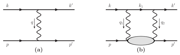
Figure 1: Contributions to elastic electron–nucleon scattering from (a) one-photon exchange, and (b) two-photon exchange amplitudes, with particle momenta as indicated. For TPE we have $q_{1}+q_{2}=q$. Only the $s$-channel “box” diagram is drawn. The “crossed-box” contribution, which can be obtained by applying crossing symmetry $s\to u$, is implied.

The elastic scattering cross section can be defined in terms of any two of the dimensionless quantities

$$\varepsilon =\frac{\nu^{2}-\tau(1+\tau)}{\nu^{2}+\tau(1+\tau)}=\frac{2\left(M^{4}-su\right)}{s^{2}+u^{2}-2M^{4}}\,,$$ (2)

$$\tau =\frac{Q^{2}}{4M^{2}}\,,\qquad\nu=\frac{k\cdot p}{M^{2}}-\tau\,.$$

The inverse relationships are also useful,

$$\nu =\frac{s-u}{4M^{2}}=\sqrt{\frac{\tau(1+\tau)(1+\varepsilon)}{1-\varepsilon}}\,,$$ (3)

$$s =M^{2}(1+2\tau+2\nu)\,.$$

In the target rest frame the variables are given by

$$\varepsilon =\left(1+2(1+\tau)\tan^{2}{\frac{\theta_{e}}{2}}\right)^{-1}\,,$$ (4)

$$\tau =\frac{E-E^{\prime}}{2M}\,,\quad\nu=\frac{E+E^{\prime}}{2M}\,,\quad E=M(\tau+\nu)\,,$$

where $E$ $(E^{\prime})$ is the energy of the incident (scattered) electron, $\theta_{e}$ is the electron scattering angle, and $\varepsilon$ ($0<\varepsilon<1$) is identified with the relative flux of longitudinal virtual photons.

II.1.1 One-photon exchange

In the Born (OPE) approximation the electron–nucleon scattering invariant amplitude can be written as

$${\cal M}_{\gamma}=-\frac{e^{2}}{q^{2}}\,j_{\mu}^{\gamma}\,J_{\gamma}^{\mu}\,,$$ (5)

where $e$ is the electric charge, and the matrix elements of the electromagnetic leptonic and hadronic currents are given in terms of the lepton ($u_{e}$) and nucleon ($u_{N}$) spinors by

$$j_{\mu}^{\gamma} =\bar{u}_{e}(k^{\prime})\,\gamma_{\mu}\,u_{e}(k)\,,$$ (6)

$$J_{\gamma}^{\mu} =\bar{u}_{N}(p^{\prime})\,\Gamma^{\mu}(q)\,u_{N}(p)\,.$$

The electromagnetic hadron current operator $\Gamma^{\mu}$ is parametrized by the Dirac ($F_{1}$) and Pauli ($F_{2}$) form factors as

$$\Gamma^{\mu}(q)=F_{1}(Q^{2})\,\gamma^{\mu}\ +\ F_{2}(Q^{2})\,\frac{i\sigma^{\mu\nu}q_{\nu}}{2M}\,,$$ (7)

where the Born form factors are functions of a single variable, $Q^{2}$. In our convention, the reduced Born cross section $\sigma_{R}^{\rm Born}$ is given by

$$\sigma_{R}^{\rm Born}=\varepsilon\,G_{E}^{2}(Q^{2})\ +\tau\,G_{M}^{2}(Q^{2})\,,$$ (8)

where the Sachs electric and magnetic form factors $G_{E,M}(Q^{2})$ are defined in terms of the Dirac and Pauli form factors as

$$G_{E}(Q^{2}) =F_{1}(Q^{2})-\tau F_{2}(Q^{2})\,,$$ (9)

$$G_{M}(Q^{2}) =F_{1}(Q^{2})+F_{2}(Q^{2})\,.$$

II.1.2 Two-photon exchange

Using the kinematics illustrated in the box diagram in Fig. 1(b), the contribution to the TPE box amplitude from an intermediate hadronic state $R$ of invariant mass $M_{R}$ can be written in the general form Blunden et al. (2003); Kondratyuk et al. (2005)

$${\cal M}_{{\gamma\gamma}}^{\rm box}=-ie^{4}\int\frac{d^{4}q_{1}}{(2\pi)^{4}}\ \frac{L_{\mu\nu}H_{R}^{\mu\nu}}{(q_{1}^{2}-\lambda^{2})(q_{2}^{2}-\lambda^{2})}\,,$$ (10)

with $q_{2}=q-q_{1}$, and an infinitesimal photon mass $\lambda$ is introduced to regulate any infrared divergences. (In general the mass $M_{R}$ can have a distribution $W$ which can be integrated over, but here we specialize to the case of a narrow state $R$.) The leptonic and hadronic tensors here are given by

$$L_{\mu\nu} = \bar{u}_{e}(k^{\prime})\,\gamma_{\mu}\,S_{F}(k_{1},m_{e})\,\gamma_{\nu}\,u_{e}(k)\,,$$ (11)

$$H_{R}^{\mu\nu} = \bar{u}_{N}(p^{\prime})\,\Gamma_{R\to\gamma N}^{\mu\alpha}(p_{R},-q_{2})\,S_{\alpha\beta}(p_{R},M_{R})\,\Gamma_{\gamma N\to R}^{\beta\nu}(p_{R},q_{1})\,u_{N}(p)\,,$$ (12)

with $k_{1}=k-q_{1}$, $p_{R}=p+q_{1}$, and the electron propagator is

$$S_{F}(k_{1},m_{e})=\frac{(\not{k}_{1}+m_{e})}{(k_{1}^{2}-m_{e}^{2}+i0^{+})}\,.$$ (13)

The hadronic transition current operator $\gamma N\to R$ is written in a general form $\Gamma_{\gamma N\to R}^{\alpha\mu}(p_{R},q)$ that allows for a possible dependence on the incoming momentum $q$ of the photon and the outgoing momentum $p_{R}$ of the hadron, while $\mu$ and $\alpha$ are Lorentz indices.

The hadronic state propagator $S_{\alpha\beta}(p_{R},M_{R})$ in this work will describe the propagation of a baryon with either spin-$\nicefrac{{1}}{{2}}$ or spin-$\nicefrac{{3}}{{2}}$. For spin-$\nicefrac{{1}}{{2}}$ intermediate states, such as the nucleon, this reduces to

$$S_{\alpha\beta}(p_{R},M_{R})\ =\ \delta_{\alpha\beta}\,S_{F}(p_{R},M_{R}),$$ (14)

and the transition operator $\Gamma_{\gamma N\to R}$ involves one free Lorentz index. For spin-$\nicefrac{{3}}{{2}}$ intermediate states, such as the $\Delta$ baryon, the propagator can be written

$$S_{\alpha\beta}(p_{R},M_{R})\ =\ -S_{F}(p_{R},M_{R})\,{\cal P}^{3/2}_{\alpha\beta}(p_{R}),$$ (15)

where the projection operator

$${\cal P}^{3/2}_{\alpha\beta}(p_{R})\ =\ g_{\alpha\beta}\ -\ {1\over 3}\gamma_{\alpha}\gamma_{\beta}\ -\ {1\over 3p_{R}^{2}}\left(\not{p}_{R}\gamma_{\alpha}(p_{R})_{\beta}+(p_{R})_{\alpha}\gamma_{\beta}\not{p}_{R}\right)\,,$$ (16)

ensures the presence of only spin-$\nicefrac{{3}}{{2}}$ components. Unphysical spin-$\nicefrac{{1}}{{2}}$ contributions are suppressed by the condition on the vertex $p_{R\alpha}\Gamma_{\gamma N\to R}^{\alpha\mu}(p_{R},q)=0$.

One can obtain the crossed-box (“xbox”) contribution directly from the box term (10) by applying crossing symmetry. For example, in the unpolarized case, we have

$${\cal M}_{{\gamma\gamma}}^{\rm xbox}(u,t)=-{\cal M}_{{\gamma\gamma}}^{\rm box}(s,t)\Big{|}_{s\to u}\,.$$ (17)

In general, ${\cal M}_{{\gamma\gamma}}^{\rm box}(s,t)$ has both real and imaginary parts, whereas ${\cal M}_{{\gamma\gamma}}^{\rm xbox}(u,t)$ is purely real. The total squared amplitude for the sum of the one- and two-photon exchange processes shown in Fig. 1 is then

$$\left|{\cal M}_{\gamma}+{\cal M}_{{\gamma\gamma}}\right|^{2} \approx\left|{\cal M}_{\gamma}\right|^{2}+2\operatorname{Re}\left({\cal M}_{\gamma}^{\dagger}{\cal M}_{{\gamma\gamma}}\right)$$ (18)

$$\equiv\left|{\cal M}_{\gamma}\right|^{2}\left(1+\delta_{\rm TPE}\right),$$

where the relative correction to the cross section due to the interference of the one- and two-photon exchange amplitudes is defined as

$$\delta_{\rm TPE}=\frac{2\operatorname{Re}\left({\cal M}_{\gamma}^{\dagger}{\cal M}_{{\gamma\gamma}}\right)}{\left|{\cal M}_{\gamma}\right|^{2}}\,.$$ (19)

Within the framework of the simplest hadronic models, analytic evaluation of $\delta_{\rm TPE}$ is made possible by writing the transition form factors at the $\gamma$-hadron vertices as a sum and/or product of monopole form factors Blunden et al. (2003, 2005), which are typically fit to empirical transition form factors over a suitable range in spacelike four-momentum transfer. Four-dimensional integrals over the momentum in the one-loop box diagram can then be expressed in terms of the Passarino-Veltman (PV) scalar functions $A_{0}$, $B_{0}$, $C_{0}$ and $D_{0}$ ’t Hooft and Veltman (1979); Passarino and Veltman (1979). This reduction to scalar integrals is automated by programs such as FeynCalc Mertig et al. (1991); Shtabovenko et al. (2016). The PV functions can then be evaluated numerically using packages such as LoopTools Hahn and Perez-Victoria (1999). In this paper we are interested only in the imaginary parts of these PV functions, which are considerably simpler than the full expressions. This will be discussed in detail in the next section.

Note that the expressions (10) and (19) contain infrared (IR) divergences arising from the elastic intermediate state when the momentum $q_{i}\ (i=1,2)$ of either photon vanishes. In analyzing the TPE corrections for $ep$ scattering, it is convenient to subtract off these conventional IR-divergent parts, which are independent of hadronic structure, and which are usually already included in experimental analyses using a specific prescription (e.g. Mo & Tsai Mo and Tsai (1969), Grammer & Yennie Grammer and Yennie (1973), or Maximon & Tjon Maximon and Tjon (2000)).

In general, the TPE amplitude at the IR poles ($q_{1}\to 0$ or $q_{2}\to 0$) has the form

$${\cal M}_{\gamma\gamma}\longrightarrow{\cal M}_{\gamma}\Delta_{\rm IR}\,,$$ (20)

where $\Delta_{\rm IR}$ is a function containing all the IR divergences that is independent of hadronic structure. Its form depends on the particular IR prescription being used. This is discussed extensively in the TPE review by Arrington, Blunden, and Melnitchouk Arrington et al. (2011), and we defer to that paper for details. The hard-TPE correction of interest is then

$$\delta_{{\gamma\gamma}}\equiv\delta_{\rm TPE}-2\operatorname{Re}\Delta_{\rm IR}\,.$$ (21)

In this paper we follow the prescription used by Maximon and Tjon Maximon and Tjon (2000), which is to evaluate the contribution to the numerator of Eq. (10) arising from the poles $q_{i}\to 0$, while keeping the propagators in the denominator intact. In this prescription,

$$\Delta_{\rm IR}({\rm MTj})=-\frac{\alpha}{\pi}\log\left(\frac{M^{2}-s}{M^{2}-u}\right)\log\left(\frac{Q^{2}}{\lambda^{2}}\right)\,.$$ (22)

This expression has both real and imaginary parts. In our convention, $\log(-x)=\log{x}-i\pi$ for $x>0$, so explicitly the real and imaginary parts are

$$\operatorname{Re}\Delta_{\rm IR}({\rm MTj}) = -\frac{\alpha}{\pi}\log\left(\frac{s-M^{2}}{M^{2}-u}\right)\log\left(\frac{Q^{2}}{\lambda^{2}}\right)\,,$$ (23a)

$$\operatorname{Im}\Delta_{\rm IR}({\rm MTj}) = \alpha\log\left(\frac{Q^{2}}{\lambda^{2}}\right)\,.$$ (23b)

After accounting for conventional radiative corrections, the measured reduced cross section $\sigma_{R}$ is related to the Born cross section by

$$\sigma_{R}=\sigma_{R}^{\rm Born}\left(1+\delta_{{\gamma\gamma}}\right)\,.$$ (24)

In practice, most experimental cross section analyses use the IR-divergent expression of Mo and Tsai Mo and Tsai (1969), so that if one uses the Maximon and Tjon prescription Maximon and Tjon (2000) (as we do in this paper) then the difference should be accounted for when comparing to experimental data (see Ref. Arrington et al. (2011) for further discussion).

The total TPE amplitude ${\cal M}_{{\gamma\gamma}}$ can be rewritten in terms of “generalized form factors”, generalizing the expressions of Eqs. (5)–(7), as described by Guichon and Vanderhaeghen Guichon and Vanderhaeghen (2003). Although the decomposition is not unique, and different generalized form factor conventions have been used in the literature, in this paper we use the basis of form factors denoted by $F_{1}^{\prime}$, $F_{2}^{\prime}$ and $G_{a}^{\prime}$, defined via

$${\cal M}_{\gamma\gamma} = -{e^{2}\over q^{2}}\,\bar{u}_{e}(k^{\prime})\gamma_{\mu}u_{e}(k)\ \bar{u}_{N}(p^{\prime})\left[F_{1}^{\prime}(Q^{2},\nu)\,\gamma^{\mu}\,+\,F_{2}^{\prime}(Q^{2},\nu)\,{i\sigma^{\mu\nu}q_{\nu}\over 2M}\right]u_{N}(p)$$ (25)

$$-{e^{2}\over q^{2}}\,\bar{u}_{e}(k^{\prime})\gamma_{\mu}\gamma_{5}u_{e}(k)\,\bar{u}_{N}(p^{\prime})\,G_{a}^{\prime}(Q^{2},\nu)\,\gamma^{\mu}\gamma_{5}u_{N}(p)\,,$$

where the vector $F_{1}^{\prime}$ and $F_{2}^{\prime}$ generalized form factors are the TPE analogs of the Dirac and Pauli form factors, while the axial vector $G_{a}^{\prime}$ generalized form factor has no Born level analog.

Rather than construct $\delta_{\rm TPE}$ and subtract the IR-divergent terms, as in Eq. (21), it is convenient to incorporate the IR subtractions directly into the generalized form factors $F_{1}^{\prime}$ and $F_{2}^{\prime}$ ($G_{a}^{\prime}$ is not IR-divergent),

$$F_{1}^{\prime} \equiv F_{1,{\rm TPE}}^{\prime}-F_{1}(Q^{2})\,\Delta_{\rm IR}\,,$$ (26a)

$$F_{2}^{\prime} \equiv F_{2,{\rm TPE}}^{\prime}-F_{2}(Q^{2})\,\Delta_{\rm IR}\,,$$ (26b)

where $F_{i,{\rm TPE}}^{\prime}$ refer to the unregulated expressions. In terms of these regulated generalized form factors, the relative TPE correction is given by

$$\delta_{\gamma\gamma}=2\operatorname{Re}\frac{\varepsilon G_{E}(F_{1}^{\prime}-\tau F_{2}^{\prime})+\tau G_{M}(F_{1}^{\prime}+F_{2}^{\prime})+\nu(1-\varepsilon)G_{M}G_{a}^{\prime}}{\varepsilon G_{E}^{2}+\tau G_{M}^{2}}\,.$$ (27)

II.2 Dispersive approach

As noted earlier, the TPE amplitude ${\cal M}_{\gamma\gamma}$ has both real and imaginary parts. The real and imaginary parts can be related through dispersion relations Gorchtein (2007); Borisyuk and Kobushkin (2008), which forms the basis of the dispersive method discussed in this section. Our discussion in this section follows the formalism of Tomalak and Vanderhaeghen Tomalak and Vanderhaeghen (2014, 2015). An alternative treatment by Borisyuk and Kobushkin Borisyuk and Kobushkin (2008) starts from the annihilation channel, $e^{-}+e^{+}\to p+\bar{p}$.

Using the parametrization of the TPE amplitude ${\cal M}_{\gamma\gamma}$ in terms of the generalized form factors $F_{1}^{\prime}$, $F_{2}^{\prime}$ and $G_{a}^{\prime}$, we note that these TPE amplitudes have the symmetry properties Gorchtein (2007); Borisyuk and Kobushkin (2008)

$$F_{1,2}^{\prime}(Q^{2},-\nu) = -F_{1,2}^{\prime}(Q^{2},\nu)\,,$$ (28a)

$$G_{a}^{\prime}(Q^{2},-\nu) = +G_{a}^{\prime}(Q^{2},\nu)\,,$$ (28b)

and satisfy the fixed-$t$ dispersion relations

$$\operatorname{Re}F_{1}^{\prime}(Q^{2},\nu) = \frac{2}{\pi}{\cal P}\int_{\nu_{\rm th}}^{\infty}d\nu^{\prime}\ {\nu\over\nu^{\prime 2}-\nu^{2}}\,\operatorname{Im}F_{1}^{\prime}(Q^{2},\nu^{\prime})\,,$$ (29a)

$$\operatorname{Re}F_{2}^{\prime}(Q^{2},\nu) = \frac{2}{\pi}{\cal P}\int_{\nu_{\rm th}}^{\infty}d\nu^{\prime}\ {\nu\over\nu^{\prime 2}-\nu^{2}}\,\operatorname{Im}F_{2}^{\prime}(Q^{2},\nu^{\prime})\,,$$ (29b)

$$\operatorname{Re}G_{a}^{\prime}(Q^{2},\nu) = \frac{2}{\pi}{\cal P}\int_{\nu_{\rm th}}^{\infty}d\nu^{\prime}\ {\nu^{\prime}\over\nu^{\prime 2}-\nu^{2}}\,\operatorname{Im}G_{a}^{\prime}(Q^{2},\nu^{\prime})\,.$$ (29c)

Here ${\cal P}$ denotes the Cauchy principal value integral, and $\nu_{\rm th}=-\tau$ is the threshold for the elastic cut, corresponding to an electron of energy $E=0$. The physical threshold for electron scattering is at $\varepsilon=0$ (or $\cos\theta_{e}=-1$), which requires $E\geq M(\tau+\nu_{\rm ph})$, with $\nu_{\rm ph}\equiv\sqrt{\tau(1+\tau)}$. This integral therefore extends into an unphysical region of parameter space, which requires knowledge of the transition form factors in the timelike region of four-momentum transfer. The crossed-box terms in the real part of the TPE amplitudes are generated by incorporating the symmetry properties into the dispersive integrals, which is equivalent to the use of Eq. (17) in the loop calculation.

For the interaction of point particles, such as in elastic $e\mu$ scattering, the real parts generated in this way agree completely with those obtained directly from the four-dimensional loop integrals of Eq. (10) Tomalak and Vanderhaeghen (2014). In general, however, there may be momentum dependence in the $\gamma$-hadron interaction, such as for the $\gamma N\Delta$ vertex (see Sec. III.2 below). In fact, the momentum dependence in a transition vertex function allows one to construct different parametrizations of that vertex function, for example, by using the Dirac equation, that are equivalent on-shell but differ off-shell. The additional momentum-dependence associated with this freedom will affect one-loop integrals because the intermediate hadronic states are not on-shell. This ambiguity is not present in the dispersive method, for which all the intermediate states are on-shell. In the context of TPE, this means that for any momentum-dependent interactions one should not expect agreement between the real parts of the generalized form factors calculated from Eqs. (29) and those calculated using the loop integration method. We will quantify these differences for the cases of the nucleon and $\Delta$ intermediate states in Sec. III.

II.2.1 Analytic method

The analytic approach used in previous work Blunden et al. (2003); Kondratyuk et al. (2005); Blunden et al. (2005); Kondratyuk and Blunden (2007); Tjon and Melnitchouk (2008); Nagata et al. (2009); Tjon et al. (2009); Graczyk (2013); Lorenz et al. (2015); Zhou and Yang (2015) relies on a parameterization of the transition form factors as a sum and/or product of monopole form factors. The most basic relation is

$$\frac{1}{q_{i}^{2}}\left(\frac{\Lambda_{i}^{2}}{\Lambda_{i}^{2}-q_{i}^{2}}\right)=\frac{1}{q_{i}^{2}}-\frac{1}{q_{i}^{2}-\Lambda_{i}^{2}}\,,$$ (30)

which is to be applied at each photon–hadron vertex ($i=1,2$). More complicated constructions are straightforward to generate by repeatedly applying the feature that the product of any two monopoles is proportional to their difference. The general expression for an amplitude with form factors will thus involve a sum of “primitive” integrals with different photon mass parameters $\Lambda_{1}$ and $\Lambda_{2}$ for each of the two photon propagators, modified according to Eq. (30). The primitive integrals may yield spurious ultraviolet or infrared divergences, but these divergences will cancel when taking the sum. We give details on these constructions in Appendix B.

By means of the PV reduction scheme, a one-loop integral for the box-diagram amplitude can be written in terms of a set of scalar PV functions $A_{0}$, $B_{0}$, $C_{0}$ and $D_{0}$, corresponding to one-, two-, three-, and four-point functions. This can be visualized as a “pinching” of the four various propagators in the box diagram due to cancellations of the terms in the numerator with the propagator terms in the denominator. The PV functions can be evaluated numerically, and there are various computer programs to do this Hahn and Perez-Victoria (1999); van Hameren (2011); Carrazza et al. (2016); Denner et al. (2017).

In general the scalar PV functions are complex-valued. The imaginary parts of the TPE amplitudes are contained entirely in these functions. For the box (and crossed-box) diagrams in elastic $ep$ scattering there are only four of the PV functions that have imaginary parts. These four functions are the ones that arise in the $s$-channel box diagram with the electron and intermediate hadronic states on-shell. This is illustrated in Fig. 2.

Figure 2: Visualization of the Passarino-Veltman functions from the TPE amplitudes that have an imaginary part, for (a) $b_{0}(s)$; (b) $c_{0}(s;\Lambda)$; (c) $d_{0}(s;\Lambda_{1},\Lambda_{2})$, where $s$ is the total invariant mass of the system. Here external legs have been amputated. The double line indicates a hadronic state of invariant mass $W$, and the dotted line indicates that the electron and hadronic states are on-shell. For elastic scattering, $c_{0}(s;\Lambda)$ is the same whichever photon propagator is pinched, and $d_{0}(s;\Lambda_{2},\Lambda_{1})=d_{0}(s;\Lambda_{1},\Lambda_{2})$.

Recall that an amplitude becomes imaginary when the intermediate state particles become real, or on their mass shells. This is formalized by the well-known Cutkosky cutting rules Cutkosky (1958). Namely, as a consequence of unitarity, the imaginary part of a scattering amplitude can be obtained by summing all possible cuttings of the corresponding Feynman diagram, where a cut is across any two internal propagators separating the external states from the rest of the diagram. Cut propagators are then put on-shell according to the rule $1/(p^{2}-m^{2}+i0^{+})\ \to\ -2\pi i\,\theta(p_{0})\,\delta(p^{2}-m^{2})$.

For elastic scattering, the two functions $C_{0}(s)$ arising when either photon propagator is pinched are identical, so there are only three distinct PV functions. Other PV functions where the electron or hadronic intermediate state (or both) are pinched have no imaginary parts for $ep$ scattering, and the $u$-channel crossed-box diagram also has no imaginary part. (Recall that the crossed-box amplitude can be obtained by replacing $s\to u$, with an appropriate overall changed in sign given in Eq. (28).) We will denote these three functions as $B_{0}(s)$, $C_{0}(s;\Lambda_{1})$, and $D_{0}(s;\Lambda_{1},\Lambda_{2})$. The full expression for these functions is

$$\left\{B_{0}(s),C_{0}(s;\Lambda_{1}^{2}),D_{0}(s;\Lambda_{1}^{2},\Lambda_{2}^{2})\right\}\equiv\frac{1}{i\pi^{2}}\,\int d^{4}q_{1}$$

$$\hskip 113.81102pt\times\left\{1,\frac{1}{\left(q_{1}^{2}-\Lambda_{1}^{2}\right)},\frac{1}{\left(q_{1}^{2}-\Lambda_{1}^{2}\right)\left(q_{2}^{2}-\Lambda_{2}^{2}\right)}\right\}$$

$$\hskip 113.81102pt\times\frac{1}{\left[(k-q_{1})^{2}-m_{e}^{2}+i0^{+}\right]\left[(p+q_{1})^{2}-W^{2}+i0^{+}\right]}\,.$$

In addition to the explicit dependence on $s$ and $\Lambda_{i}^{2}$, there is also an implied dependence on $M$, $W$, and $Q^{2}$ that is suppressed for clarity of notation (see Appendix B for details).

We define the imaginary parts of the PV functions by $\{b_{0}(s),c_{0}(s),d_{0}(s)\}\equiv\{\operatorname{Im}B_{0}(s),\operatorname{Im}C_{0}(s),\operatorname{Im}D_{0}(s)\}$. According to the Cutkosky rules, the imaginary parts correspond to putting the electron and intermediate hadronic states on-shell, $k_{1}^{2}\equiv(k-q_{1})^{2}=m_{e}^{2}$ and $(p+q_{1})^{2}=W^{2}$. Working in the center-of-mass (CM) frame, we define the electron variables

$$k = E_{k}(1;0,0,1),$$

$$k^{\prime} = E_{k}(1;\sin\theta,0,\cos\theta),$$ (32)

$$k_{1} = E_{k_{1}}(1;\sin\theta_{k_{1}}\cos\phi_{k_{1}},\sin\theta_{k_{1}}\sin\phi_{k_{1}},\cos\theta_{k_{1}}).$$

In this frame we have

$$E_{k}=\frac{s_{M}}{2\sqrt{s}}\,,\quad E_{k_{1}}=\frac{s_{W}}{2\sqrt{s}}\,,\quad\cos\theta=1-\frac{Q^{2}}{2E_{k}^{2}}\,,$$ (33)

with the shorthand notation

$$s_{M}\equiv(s-M^{2})\,,\qquad s_{W}\equiv(s-W^{2})\,.$$ (34)

In the physical region, the CM scattering angle $\theta$ satisfies the constraint $-1\leq\cos\theta\leq 1$, requiring $s_{M}^{2}\geq sQ^{2}$. However, the dispersive integral of Eq. (29) only requires $s_{M}>0$, meaning there is an unphysical region of parameter space where $\cos\theta<-1$, and $\sin\theta$ is purely imaginary. Therefore, in the dispersive approach expressions for the imaginary parts of the TPE amplitudes need to be analytically continued into this unphysical region.

Recall that in terms of the electron energy in the laboratory frame, $E$, the $ep$-invariant mass squared is $s=M^{2}+2ME$. After changing the integration variable from $q_{1}$ to $k_{1}$, and using the on-shell conditions, we find after some algebra the expressions

$$\left\{b_{0}(s),c_{0}(s;\Lambda_{1}^{2}),d_{0}(s;\Lambda_{1}^{2},\Lambda_{2}^{2})\right\}\equiv\frac{s_{W}}{4s}\theta(s_{W})$$ (35)

$$\times\int d\Omega_{k_{1}}\left\{1,\frac{-1}{\left(Q_{1}^{2}+\Lambda_{1}^{2}\right)},\frac{1}{\left(Q_{1}^{2}+\Lambda_{1}^{2}\right)\left(Q_{2}^{2}+\Lambda_{2}^{2}\right)}\right\}\,,$$

where $Q_{i}^{2}=-q_{i}^{2}$ are the squared four-momenta of the virtual photons ($i=1,2$), with

$$Q_{1}^{2} =Q_{0}^{2}\left(1-\cos\theta_{k_{1}}\right),$$ (36)

$$Q_{2}^{2} =Q_{0}^{2}\left(1-\cos\theta\cos\theta_{k_{1}}-\sin\theta\sin\theta_{k_{1}}\cos\phi_{k_{1}}\right),$$

and $Q_{0}^{2}=2E_{k}E_{k_{1}}=s_{M}s_{W}/(2s)$.

The $b_{0}$ integral in Eq. (35) is trivial. Through the use of Eq. (36), the other integrals can be brought into the form

$$J=\int d\Omega_{k_{1}}\,\frac{1}{(a_{1}-b_{1}\cos\theta_{k_{1}})(a_{2}-b_{2}\cos\theta_{k_{1}}-c_{2}\sin\theta_{k_{1}}\cos\phi_{k_{1}})}\,.$$ (37)

The integrand here has poles when $|b_{2}|>|a_{2}|$, which can arise in the unphysical region when $Q_{2}^{2}$ becomes timelike. A simpler version of this integral was considered by Mandelstam Mandelstam (1958) for the case where the target and scattering particles have equal masses. The general expression has been given by Beenakker and Denner Beenakker and Denner (1990),

$$J = \frac{2\pi}{X}\,\log\left(\frac{a_{1}a_{2}-b_{1}b_{2}+X}{a_{1}a_{2}-b_{1}b_{2}-X}\right)\,,$$ (38)

$${\rm with}\quad X^{2} = (a_{1}a_{2}-b_{1}b_{2})^{2}-(a_{1}^{2}-b_{1}^{2})(a_{2}^{2}-b_{2}^{2}-c_{2}^{2})\,.$$

For the $c_{0}(s)$ function, we set $a_{1}=1+\Lambda_{1}^{2}/Q_{0}^{2}$, $b_{1}=1$, $a_{2}=1$, $b_{2}=0$, and $c_{2}=0$. For $d_{0}(s)$, we set $a_{i}=1+\Lambda_{i}^{2}/Q_{0}^{2}$, $b_{1}=1$, $b_{2}=\cos\theta$, and $c_{2}=\sin\theta=\sqrt{1-b_{2}^{2}}$. In the unphysical region, $\cos\theta<-1$, so that $\sin\theta$ is purely imaginary. However, we note that the combination $b_{2}^{2}+c_{2}^{2}=1$, and therefore $0\leq X\leq(a_{1}a_{2}-b_{1}b_{2})$, independent of the value of $\cos\theta$. Thus Eq. (38) for $J$ is the proper analytic continuation of the integral for $d_{0}(s)$ into the unphysical region. Explicit expressions for $b_{0}(s)$, $c_{0}(s;\Lambda)$ and $d_{0}(s;\Lambda_{1},\Lambda_{2})$, including the IR limits $\Lambda\to\lambda$, are given in Appendix B.

In previous work Blunden et al. (2003, 2005) the TPE amplitudes were obtained by numerical evaluation of the PV functions using the program LoopTools Hahn and Perez-Victoria (1999). The real parts were used directly, and the imaginary parts were not needed. Here, we have constructed analytic expressions for the imaginary parts in terms of elementary logarithms, thus allowing a completely analytic evaluation of the imaginary parts of the TPE amplitudes. The real parts are then constructed from a numerical evaluation of the dispersion integrals of Eq. (29). The imaginary parts obtained here are, of course, identical with those obtained numerically in the earlier work Blunden et al. (2003, 2005). The real parts are numerically identical for the elastic $F_{1}^{\prime}$ and $F_{2}^{\prime}$ TPE amplitudes, while the $G_{a}^{\prime}$ amplitude differs, but in a numerically insignificant way. For the inelastic $\Delta$ states there are significant differences, especially as $\varepsilon\to 1$. These differences will be discussed further in Sec. III.

As an alternative to using the PV reduction method implemented in FeynCalc Mertig et al. (1991); Shtabovenko et al. (2016), one can work entirely with on-shell quantities. Using the on-shell conditions, we find that the TPE amplitudes are sums of integrals of the general form

$$I=\frac{s_{W}}{4s}\int\,d\Omega_{k_{1}}\ \frac{f\left(Q_{1}^{2},Q_{2}^{2}\right)}{\left(Q_{1}^{2}+\lambda^{2}\right)\left(Q_{2}^{2}+\lambda^{2}\right)}\frac{\Lambda_{1}^{2}}{Q_{1}^{2}+\Lambda_{1}^{2}}\frac{\Lambda_{2}^{2}}{Q_{2}^{2}+\Lambda_{2}^{2}}\,,$$ (39)

where $f(Q_{1}^{2},Q_{2}^{2})$ is a polynomial function of combined degree $N$ in $Q_{1}^{2}$ and $Q_{2}^{2}$,

$$f(Q_{1}^{2},Q_{2}^{2})=\sum_{i=0}^{N}\,\sum_{j=0}^{N-i}\ f_{ij}\,Q_{1}^{2i}\,Q_{2}^{2j}\,.$$ (40)

The coefficients $f_{ij}$ are functions of $s$, $W$, and $Q^{2}$, and satisfy $f_{ij}=f_{ji}$ for elastic scattering due to the symmetry under $Q_{1}^{2}\leftrightarrow Q_{2}^{2}$. Thus we can write

$$I=\sum_{i=0}^{N}\,\sum_{j=0}^{N-i}\ f_{ij}I_{ij}\,,$$ (41)

with the “primitive” integrals $I_{ij}$ defined as

$$I_{ij}=\frac{s_{W}}{4s}\int\,d\Omega_{k_{1}}\ \frac{Q_{1}^{2i}Q_{2}^{2j}}{\left(Q_{1}^{2}+\lambda^{2}\right)\left(Q_{2}^{2}+\lambda^{2}\right)}\frac{\Lambda_{1}^{2}}{Q_{1}^{2}+\Lambda_{1}^{2}}\frac{\Lambda_{2}^{2}}{Q_{2}^{2}+\Lambda_{2}^{2}}\,.$$ (42)

For nucleon intermediate states we find $N=2$, indicating that monopole form factors are sufficient to eliminate the UV divergences (there is one power of $q_{i}$ at each photon–nucleon vertex in the $F_{2}$ term of $\Gamma^{\mu}(q_{i})$). For $\Delta$ intermediate states, however, we find $N=3$, which implies that dipole form factors (or a product of monopoles) are needed to eliminate the UV divergences, as there are up to two powers of $q_{i}$ at each vertex in $\Gamma_{\gamma N\to\Delta}^{\alpha\mu}$ (see Secs. III.1 and III.2 below). The integrals of Eq. (42) up to $N=2$ are given in Table 1 of Appendix B, and can easily be extended to more complicated form factor constructions.

II.2.2 Numerical method

In analogy with Eq. (39), the TPE amplitudes of interest have the general form

$$\frac{s_{W}}{4s}\int\,d\Omega_{k_{1}}\ \frac{f\left(Q_{1}^{2},Q_{2}^{2}\right)G_{1}(Q_{1}^{2})\,G_{2}(Q_{2}^{2})}{\left(Q_{1}^{2}+\lambda^{2}\right)\left(Q_{2}^{2}+\lambda^{2}\right)}\,,$$ (43)

where $f(Q_{1}^{2},Q_{2}^{2})$ is a polynomial function of combined degree 2 (3) in $Q_{1,2}^{2}$ for $N~{}(\Delta)$ intermediate states, and $G_{i}(Q_{i}^{2})$ are form factors that are real-valued and finite for all spacelike values of $Q_{i}^{2}$. For elastic scattering, the total integral is symmetric under the interchange $Q_{1}^{2}\leftrightarrow Q_{2}^{2}$. For the nucleon intermediate state, it is convenient to bring the IR subtractions of Eq. (26) into this integral. This is consistent with the Maximon and Tjon IR regularization scheme whereby the numerator of Eq. (43) vanishes whenever $Q_{i}^{2}\to 0$. It also vanishes for excited states under these conditions. Therefore we could actually set $\lambda\to 0$ without encountering any singularities in the integrals. This is unlike the analytic expressions of the previous section, where only the sum of individual IR-divergent expressions is independent of $\lambda$.

In the physical region there are no singularities in the integrand of Eq. (43), so evaluation of the integral is a straightforward 2-dimensional numerical quadrature over the domain $-1\leq\cos\theta_{k_{1}}\leq 1$ and $0\leq\phi_{k_{1}}\leq 2\pi$, following Eq. (36). However, this approach fails in the unphysical region. To get around this, Tomalak and Vanderhaeghen used a contour integration method Tomalak and Vanderhaeghen (2015), and applied it to the calculation of TPE amplitudes with monopole form factors. By summing the residue at the poles enclosed by the contour they were able to obtain algebraic expressions for the TPE amplitudes. These expressions are equivalent to the ones we obtained in the previous section using algebraic expressions for the PV functions. In this section we will follow this method, with modifications, to implement a numerical contour integration of Eq. (43) that allows for a more general parametrization of the transition form factors than a sum and/or product of monopoles.

In the complex $Q_{i}^{2}$ plane, we define a timelike half with $\operatorname{Re}Q_{i}^{2}<0$, and spacelike half with $\operatorname{Re}Q_{i}^{2}>0$. In general, the allowed form factors can have poles in $Q_{i}^{2}$ anywhere in the timelike half of the complex plane. With certain restrictions, which we will state explicitly, the form factors can have poles in the spacelike half as well.

Without providing a rigorous mathematical proof, we can nonetheless specify certain restrictions on the type of allowed form factors. Namely, they should have a simple functional form in $Q_{i}^{2}$, such as exponentials, polynomials, or inverse polynomials, that can be analytically continued to the complex plane. There should be no branch cuts, and any poles should either lie along the negative, real axis (at timelike $Q_{i}^{2}$), or occur in complex conjugate pairs. This is the case for a commonly used form factor parametrization [see Eq. (51)] in terms of a ratio of polynomials Kelly (2004); Arrington et al. (2007); Venkat et al. (2011).

The area of integration in Eq. (43) can be visualized as an integral over the photon virtual momenta $Q_{1}^{2}$ and $Q_{2}^{2}$ of Eq. (36), which form a symmetric ellipse in $Q_{1}^{2}$ vs. $Q_{2}^{2}$, centered at $\{Q_{0}^{2},Q_{0}^{2}\}$ Gorchtein and Horowitz (2008); Tomalak and Vanderhaeghen (2015). The boundary of the ellipse is defined by $\cos\phi_{k_{1}}=1$. Following Ref. Tomalak and Vanderhaeghen (2015), we make a change of variables to elliptic coordinates,

$$\int d\Omega_{k_{1}}\to 2\int_{0}^{1}d\alpha\int_{0}^{2\pi}d\theta_{k_{1}}\,.$$ (44)

The contours of constant $\alpha$ represent concentric ellipses with radial parameter $r=\sqrt{1-\alpha^{2}}$. From Eq. (36), in elliptic coordinates we have

$$Q_{1}^{2} =Q_{0}^{2}\left(1-r\cos\theta_{k_{1}}\right)\,,$$ (45)

$$Q_{2}^{2} =Q_{0}^{2}\left(1-r\cos\theta\cos\theta_{k_{1}}-r\sin\theta\sin\theta_{k_{1}}\right)\,.$$

In the physical region the integral over $\theta_{k_{1}}$ can be rewritten as a contour integral on the unit circle $z=\exp(i\theta_{k_{1}})$, with $Q_{i}^{2}(z)$ regarded as functions of $z$ (and $r$) using

$$\cos\theta_{k_{1}}=\frac{1}{2}\left(z+\frac{1}{z}\right)\,,\quad\sin\theta_{k_{1}}=\frac{1}{2i}\left(z-\frac{1}{z}\right)\,,$$ (46)

and

$$\int_{0}^{2\pi}d\theta_{k_{1}}\to\oint\frac{dz}{iz}\,.$$ (47)

In anticipation of extending this formalism to the unphysical region, Eq. (45) can be simplified into the form

$$Q_{1}^{2}(z) =Q_{0}^{2}\left[1-\frac{r}{2}\left(z+\frac{1}{z}\right)\right]\,,$$ (48)

$$Q_{2}^{2}(z) =Q_{0}^{2}\left[1-\frac{r}{2}\left(\frac{z}{\beta}+\frac{\beta}{z}\right)\right]\,,$$

with

$$\beta\equiv\left\{\begin{array}[]{l c l}e^{i\theta}&\mbox{ for}&-1\leq\cos\theta\leq 1\,,\\ \cos\theta-\sqrt{\cos^{2}\theta-1}&\mbox{ for}&\cos\theta<-1\,.\end{array}\right.$$ (49)

Recall that $\cos\theta$ is given in Eq. (33) in terms of $s$ and $Q^{2}$. Expressed in this way, it is clear that $Q_{1}^{2}(z)=Q_{2}^{2}(\beta z)$. Because the integrands of the full TPE amplitudes are symmetric under the interchange $Q_{1}^{2}\leftrightarrow Q_{2}^{2}$, this means that for every value $z_{1}$ associated with the poles in $Q_{1}^{2}$ in the complex $z$ plane, there is a corresponding pole at $z_{2}=\beta z_{1}$. In addition, for every pole in $Q_{1}^{2}$, both $z_{\rm 1i}$ and $z_{\rm 1o}=1/z_{\rm 1i}$ are poles in the complex $z$ plane, where $|z_{\rm 1i}|\leq 1$ lies inside the unit circle, and $|z_{\rm 1o}|\geq 1$ lies outside the unit circle. The values $z_{\rm 1i}=z_{\rm 1o}=1$ are the IR-divergent poles, where $Q_{1}^{2}=0$ for $r=1$. These could be regulated by introducing the $\lambda$ photon mass parameter, but as the integrand vanishes in our regularization scheme when $Q_{1}^{2}=0$, there is no IR divergence, and one can set $\lambda=0$. Analogously, for $Q_{2}^{2}$, both $z_{\rm 2i}$ and $z_{\rm 2o}=\beta^{2}/z_{\rm 2i}$ are poles inside and outside a circle of radius $|\beta|$, respectively. The values $z_{\rm 2i}=z_{\rm 2o}=\beta$ are the IR-divergent poles, where $Q_{2}^{2}=0$ for $r=1$. These results are valid in either the physical region, where $\beta=\exp(i\theta)$, or the unphysical region, where $\beta<-1$.

As an illustration of these points, consider the monopole form factors as given in Eq. (39), for which there is a pole in $Q_{1}^{2}$ along the negative real axis at $-\Lambda_{1}^{2}$. This yields poles $z_{\rm 1i}$ and $z_{\rm 1o}$ along the positive real axis in the complex $z$ plane, with the interior pole $z_{\rm 1i}$ lying between 0 and 1. For the corresponding poles associated with $Q_{2}^{2}$, in the physical region, with $\beta=\exp(i\theta)$, these lie along a line at angle $\theta$. In the unphysical region, with $\beta<-1$, they lie along the negative real axis, with $z_{\rm 2i}$ lying between $\beta$ and 0. A graphical representation of these results in the complex $z$ plane is shown in Fig. 3, with the dots representing the “inside” points $z_{\rm 1i}$ and $z_{\rm 2i}$, and the crosses representing the “outside” points $z_{\rm 1o}$ and $z_{\rm 2o}$.

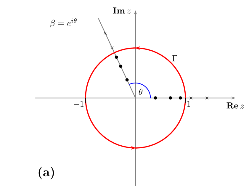
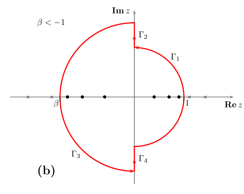
Figure 3: (a): The contour around the unit circle in the physical region, $-1\leq\cos\theta\leq 1$. For every pole $z_{\rm i}$ inside the contour (denoted by a dot), there is a corresponding pole at $z_{\rm o}=1/z_{\rm i}$ lying outside the contour (denoted by a cross). For monopole form factors, interior poles in $Q_{1}^{2}$ appear along the real $z$-axis between 0 and 1, and corresponding poles in $Q_{2}^{2}$ along the line at angle $\theta$. (b): One possible choice of contour in the unphysical region, $\cos\theta<1$, which we denote as $\Gamma_{\rm CD}$. For monopole form factors, interior poles in $Q_{1}^{2}$ lie along the real $z$-axis between 0 and 1, and corresponding poles in $Q_{2}^{2}$ lie between $\beta$ and 0.

For more general form factors, we restrict ourselves in the first instance to those functions with poles in the timelike half of the complex $Q_{i}^{2}$ plane. In this case it can be shown that all poles in $z_{\rm 1i}$ will be clustered around the positive real axis, with $|z_{\rm 1i}|\leq 1$ and $\operatorname{Re}z_{\rm 1i}>0$. Recall that for every pole $z_{1}$ there is a corresponding pole $z_{2}=\beta z_{1}$. In the physical region, all poles in $z_{\rm 2i}$ will therefore be clustered around the line at angle $\theta$, with $|z_{\rm 2i}|\leq 1$. In the unphysical region, the $z_{\rm 2i}$ poles must therefore satisfy $|z_{\rm 2i}|<|\beta|$ and $\operatorname{Re}z_{\rm 2i}<0$.

By Cauchy’s theorem, a closed contour integral is equivalent to summing the residue at the poles of the integrand enclosed by the contour. In continuing the integral from the physical to the unphysical region, the contour $\Gamma$ must be deformed in such a way that no poles cross the boundary defined by the contour. There are many possible choices of an appropriate contour in the unphysical region. However, based on the symmetry of the poles in $z_{1}$ and $z_{2}$, as discussed above, the closed contour shown in Fig. 3(b) merits special consideration. It consists of two semicircles connected by two straight line segments, which we denote as $\Gamma_{\rm CD}$. It clearly satisfies the criterion that no poles $z_{\rm 2i}$ or $z_{\rm 2o}$ cross the boundary of the contour, provided that the form factors only have poles in the timelike region of the $Q_{i}^{2}$ plane. Moreover, because of the symmetry of the TPE amplitudes under the interchange of $Q_{1}^{2}$ and $Q_{2}^{2}$, the line integrals along the contours $\Gamma_{1}$ and $\Gamma_{3}$ are equal, as are the line integrals along the contours $\Gamma_{2}$ and $\Gamma_{4}$. Furthermore, the real part of the integrand is symmetric between the upper and lower half planes, while the imaginary part is antisymmetric (hence the imaginary part integrates to 0 in any closed contour). Thus one only needs to compute the real part of the line integral along the contour $\Gamma_{1}$ in the upper half plane, plus the contribution from $\Gamma_{2}$,

$$\oint_{\Gamma}\frac{dz}{iz}f(z)\ \longmapsto\ 4\int_{0}^{\pi/2}dt\,\operatorname{Re}\Big{\{}f(z)\big{|}_{z=e^{it}}\Big{\}}+2\int_{1}^{-\beta}dt\,\operatorname{Re}\left\{\frac{f(z)}{z}\bigg{|}_{z=it}\right\}\,.$$ (50)

Form factor parametrizations $G(Q_{i}^{2})$ are driven almost exclusively by fits to data at spacelike values of $Q_{i}^{2}$. Aside from requiring no poles along the positive real axis, typically there is little or no consideration given to the location of poles in the complex $Q_{i}^{2}$ plane. Therefore, the appearance of poles in the spacelike half of $Q_{i}^{2}$ should be regarded as a nuisance rather than a reflection of any underlying physics. Nevertheless, there are form factor parametrizations in the literature that do have such poles. For example, the ratio of polynomials,

$$G(Q_{i}^{2})=\frac{\sum_{j=0}^{N}a_{j}Q_{i}^{2j}}{\sum_{k=0}^{N+2}b_{k}Q_{i}^{2k}}\,,$$ (51)

is commonly used Kelly (2004); Arrington et al. (2007); Venkat et al. (2011). Requiring all $b_{k}\geq 0$ is sufficient to eliminate zeros in the denominator for positive real $Q_{i}^{2}$, but zeros can still occur in complex conjugate pairs with $\operatorname{Re}Q_{i}^{2}>0$.

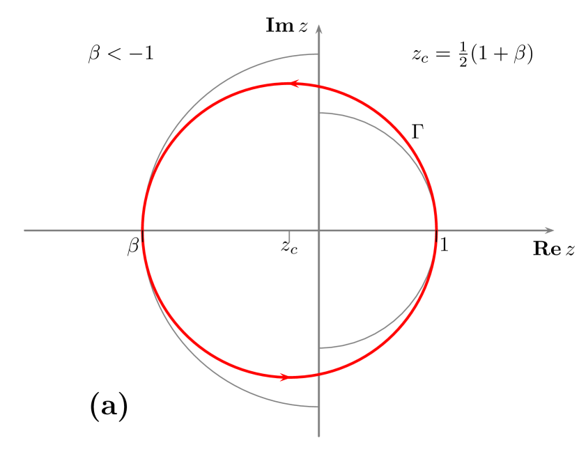
Figure 4: (a): The circular contour $\Gamma$ (shown in red) in the unphysical region is valid for form factors having poles $Q_{p}^{2}$ satisfying the condition $R>\cos\eta$, where $Q_{p}^{2}/Q^{2}=Re^{i\eta}$. For comparison, the light gray line is the contour $\Gamma_{\rm CD}$ of Fig. 3(b). (b): Visualization of the condition on the poles of the form factors in the complex $Q_{i}^{2}$ plane, using $Q^{2}=4$ GeV² as an example. Any form factors with poles in the shaded region of a circle centered at $\{\textstyle{\frac{1}{2}}Q^{2},0\}$ of radius $\textstyle{\frac{1}{2}}Q^{2}$ are not allowed. This will always occur for a large enough value of $Q^{2}$, since the limit $Q^{2}\to\infty$ is the whole spacelike region.

To handle such cases we modify the contour of integration in the unphysical region, $\Gamma_{\rm CD}$. We choose instead a circular contour centered at $z_{c}=\textstyle{\frac{1}{2}}(1+\beta)$ of radius $\textstyle{\frac{1}{2}}(1-\beta)$, as illustrated in Fig. 4(a). The new contour is shown in red, while the $\Gamma_{\rm CD}$ contour is in light gray. As we require no poles to cross the boundary defined by the new contour, there are two possible failures. Firstly, the poles $z_{\rm 1i}$ are no longer restricted to the positive half plane, and can lie anywhere inside a circle of unit radius. This gives the possibility of a pole $z_{\rm 1o}$ crossing into the interior of the new contour, since the only restriction is $|z_{\rm 1o}|>1$. Secondly, the corresponding poles $z_{\rm 2i}$ are no longer restricted to the negative half plane, and can lie outside the new contour, since the only restriction here is $|z_{\rm 2i}|<|\beta|$. By careful analysis of the location of the poles for arbitrary values of $\beta$ and $Q^{2}$, we have derived the following condition:

The validity of the contour defined by a circle of radius $\textstyle{\frac{1}{2}}(1-\beta)$, centered at $z_{c}=\textstyle{\frac{1}{2}}(1+\beta)$, is that the poles $Q_{p}^{2}$ in the form factor $G(Q_{i}^{2})$ must satisfy the condition

$$\left|2\frac{Q_{p}^{2}}{Q^{2}}-1\right|>1\,.$$ (52)

The condition (52) is equivalent to

$$R>\cos\eta,\quad{\rm with}\quad\frac{Q_{p}^{2}}{Q^{2}}=R\,e^{i\eta}\,.$$ (53)

This condition is satisfied for all $\cos\eta<0$ (poles in the timelike half of $Q_{i}^{2}$), and for all $R>1$. We can visualize the condition using a circle of radius $\textstyle{\frac{1}{2}}Q^{2}$, centered at $\{\textstyle{\frac{1}{2}}Q^{2},0\}$, in the complex $Q_{i}^{2}$ plane, where the poles $Q_{p}^{2}$ in the form factors must lie outside this circle. An example using $Q^{2}=4$ GeV² is shown in Fig. 4(b). If a form factor has poles in the spacelike half ($\cos\eta>0$), then the maximum $Q^{2}$ for which we can use the new contour is given by $Q_{\rm max}^{2}=|Q_{p}|^{2}/\cos\eta$.

III Impact of two-photon exchange

In this section we present the results of the numerical calculations of the TPE contributions to elastic $ep$ scattering within the dispersive approach, and discuss the differences with the traditional loop calculations with off-shell intermediate states. Including the nucleon and $\Delta$ intermediate state contributions, we compare the results with measurements of $e^{+}p$ to $e^{-}p$ cross section ratios from the recent CLAS Rimal et al. (2016), VEPP-3 Rachek et al. (2015); Nikolenko et al. (2014) and OLYMPUS Henderson et al. (1969) experiments, as well as with polarization observables sensitive to effects beyond the Born approximation Meziane et al. (2011).

III.1 Nucleon intermediate state

For the contributions to the box diagram from nucleon intermediate states, the inputs into the calculation are the proton elastic electric and magnetic form factors, $G_{E}^{p}$ and $G_{M}^{p}$. In the numerical calculations in this analysis we use the recent fit by Venkat et al. Venkat et al. (2011), which has the form of Eq. (51) with $N=3$ for both $G_{E}^{p}$ and $G_{M}^{p}$. As Fig. 5 illustrates, this fit gives similar results to other parametrizations, such as the ones by Kelly Kelly (2004) and Arrington et al. (AMT) Arrington et al. (2007). In contrast, the recent parametrization by Bernauer et al. Bernauer et al. (2010), which is based on a spline with 8 knots, displays distinctive wiggles at low $Q^{2}$ for both the electric and magnetic form factors. In Ref. Bernauer et al. (2010) a number of other functional forms were considered in fits to the world’s elastic electron–proton scattering data.

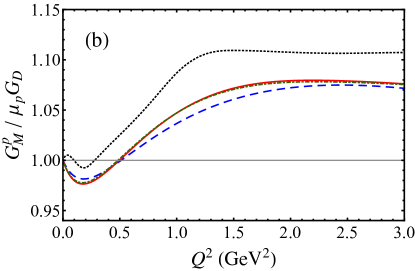
Figure 5: $Q^{2}$ dependence of the proton (a) electric and (b) magnetic form factors, scaled by the dipole form factor, $G_{D}(Q^{2})$ [see Eq. (59)], for the Kelly Kelly (2002) (dashed blue curves), Venkat et al. Venkat et al. (2011) (solid red curves), AMT Arrington et al. (2007) (dot-dashed green curves), and Bernauer et al. Bernauer et al. (2010) (dotted black curves) parametrizations.

In the application of the numerical contour integration method to the calculation of the box diagram, care must be taken to ensure that all relevant poles are included inside the contour, following the condition given in Eq. (53). For some commonly used fits in the literature, such as those by Bosted Bosted (1995) or Brash Brash et al. (2002) (in which the denominators of $G_{E}^{p}$ and $G_{M}^{p}$ are fifth-order polynomials in $\sqrt{Q^{2}}$), or the Kelly parametrization Kelly (2002) (third-order polynomials in $Q^{2}$), there are no upper limits on $Q^{2}$, since all poles occur in the timelike region. On the other hand, for the AMT Arrington et al. (2007) and Venkat et al. Venkat et al. (2011) parametrizations, which involve denominators with 5th-order polynomials in $Q^{2}$, poles in the spacelike region limit the range of applicability to $Q^{2}<4.5$ GeV². For the purposes of the data analysis in this paper, all the above parametrizations are valid; however, for future applications at higher $Q^{2}$ values care must be taken to ensure the chosen parametrization has a suitable pole structure.

The TPE contributions from nucleon intermediate states to the imaginary parts of the generalized $F_{1}^{\prime}$, $F_{2}^{\prime}$ and $G_{a}^{\prime}$ form factors are illustrated in Fig. 6 as a function of energy $E$ (in the lab frame), at a representative $Q^{2}$ value of 3 GeV². (The results at other $Q^{2}$ values are qualitatively similar.) In the low energy region, $E\lesssim 0.1$ GeV, in Fig. 6(a) the TPE amplitudes display a logarithmic divergence in $E$. Although the imaginary parts diverge, the dispersive integrals (29) for the real parts remain finite. To accommodate this in our numerical analysis, we fit the low-$E$ expressions for $\operatorname{Im}F_{1}^{\prime}$, $\operatorname{Im}F_{2}^{\prime}$ and $\operatorname{Im}G_{a}^{\prime}$ to functions of the form

$$a+b\log{E}\,,$$ (54)

with the parameters $a$ and $b$ determined by a least-squares fit for $E$ between $0.001$ and $0.01$ GeV. At high energies, the imaginary parts of the $F_{1}^{\prime}$ and $F_{2}^{\prime}$ form factors become constant, as is apparent for $E\gtrsim 6$ GeV from Fig. 6(b), where the magnified scale more clearly illustrates the asymptotic behavior. The imaginary part of the axial $G_{a}^{\prime}$ form factor falls off as $1/E$ for $E\to\infty$. This high energy behavior is sufficient to ensure the convergence of the dispersive integrals of Eq. (29). Note that the corrections to the form factors are relative to the Maximon-Tjon result for the infrared part of the TPE Maximon and Tjon (2000).

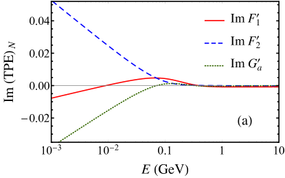
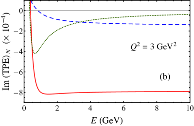
Figure 6: Imaginary parts of the TPE contributions from nucleon intermediate states to the generalized $F_{1}^{\prime}$ (solid red curves), $F_{2}^{\prime}$ (dashed blue curves) and $G_{a}^{\prime}$ (dotted green curves) form factors as a function of energy $E$, for fixed $Q^{2}=3$ GeV²: (a) illustrating the low energy behavior, $E\to 0$, and (b) showing the asymptotic behavior as large $E$.

For our numerical calculation, we compute the imaginary part of the TPE amplitudes on a logarithmic grid of 51 points in $E$, ranging up to 100 GeV. In the unphysical region, the two-dimensional numerical contour integral is computed using either of the contours discussed in the previous section, as appropriate to the poles of the form factors. In the physical region, the numerical contour integral is on the unit circle (although a direct numerical integration of (43) using Eq. (36) can also be used). We then interpolate between the grid points with a spline fit to obtain a continuous function of $E$. To obtain the real part on a grid of 20 equally spaced points in $\varepsilon$, the dispersion integral is evaluated using the $\log E$ fit for $E<0.01$ GeV, the spline fit for $0.01<E<100$ GeV, and an extrapolation beyond 100 GeV using the known asymptotic behavior. This approach can be tested against the analytic results obtained in the previous section, as well as the known analytic results for $e\mu$ scattering.

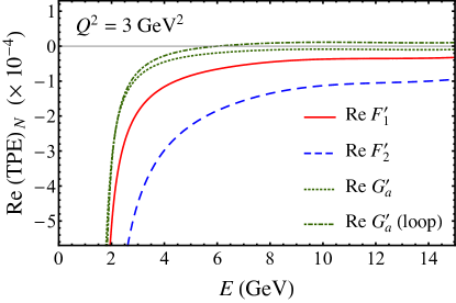
Figure 7: Dispersive results for the real parts of the TPE contributions from nucleon intermediate states to the generalized $F_{1}^{\prime}$ (solid red curve), $F_{2}^{\prime}$ (dashed blue curve) and $G_{a}^{\prime}$ (dotted green curve) form factors as a function of energy $E$, for fixed $Q^{2}=3$ GeV². The scattering threshold is at $E=1.97$ GeV. For $G_{a}^{\prime}$ the dispersive results are compared with the direct (off-shell) loop calculation (dot-dashed green curve).

Interestingly, for the real part of the TPE amplitudes the dispersive integral is dominated by contributions from the unphysical region, $E<M(\tau+\sqrt{\tau(1+\tau)})$, which for $Q^{2}=3$ GeV² is $E=1.97$ GeV. This results in the generally smoothly decaying functions for $E\gtrsim 2$ GeV observed in Fig. 7. The real parts of each of the form factors are negative in the region illustrated, with the $F_{1}^{\prime}$ form factor having the largest magnitude, and the $G_{a}^{\prime}$ form factor the smallest magnitude. Compared with the direct loop calculation in terms of the off-shell nucleon intermediate states, differences arise for the Pauli $F_{2}$ form factor term, which translates to a difference for the $G_{a}^{\prime}$ form factor. The results for the $F_{1}^{\prime}$ and $F_{2}^{\prime}$ form factors are the same for both calculations, as was observed previously in Refs. Borisyuk and Kobushkin (2008); Tomalak and Vanderhaeghen (2015). Numerically, the differences are relatively small, however, as Fig. 6 indicates, becoming notable only for $E\gtrsim 3$–4 GeV.

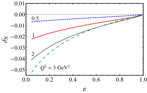
Figure 8: Dispersive TPE correction to the cross section, $\delta_{N}$, from nucleon intermediate states as a function of $\varepsilon$ for fixed values of $Q^{2}$ (= 0.5, 1, 2 and 3 GeV²). The corrections are relative to the Mo-Tsai infrared result Mo and Tsai (1969).

The total TPE correction (27) to the elastic cross section from nucleon intermediate states relative to the Mo-Tsai infrared prescription Mo and Tsai (1969), denoted $\delta_{N}$, is shown in Fig. 8 as a function of $\varepsilon$ for $Q^{2}$ between 0.5 GeV² and 3 GeV². As found in previous loop calculations Blunden et al. (2003, 2005), the corrections at these kinematics are negative, and increase in magnitude with increasing $Q^{2}$. For large $Q^{2}$ values we expect the reliability of the hadronic calculation to deteriorate, but indications from earlier work Blunden et al. (2003, 2005) suggest that it remains sizeable. In practice, since only the $G_{a}^{\prime}$ form factor is affected, and its magnitude is considerably smaller than that of $F_{1}^{\prime}$ and $F_{2}^{\prime}$, as illustrated in Fig. 7, the off-shell effects play a relatively minor role in $\delta_{N}$, with the dispersive and loop results almost indistinguishable.

III.2 $\Delta$ intermediate state

The contribution to the TPE amplitude from intermediate states involving the spin-$\nicefrac{{3}}{{2}}$, isospin-$\nicefrac{{3}}{{2}}$ $\Delta$ baryons is computed from the $\gamma^{*}N\to\Delta$ electromagnetic transition operator, $\Gamma_{\gamma N\to\Delta}^{\alpha\mu}$. Usually this is expressed in terms of three Jones-Scadron transition form factors, $G_{M}^{*}(Q^{2})$, $G_{E}^{*}(Q^{2})$ and $G_{C}^{*}(Q^{2})$, corresponding to magnetic, electric, and Coulomb multipole excitations, respectively Jones and Scadron (1973). Although the $\gamma^{*}N\to\Delta$ cross section is diagonal in these functions, they are cumbersome to work with in the transition vertex function, and other parametrizations have also been suggested in the literature Pascalutsa et al. (2007); Kondratyuk et al. (2005); Nagata et al. (2009); Pascalutsa and Tjon (2004); Caia et al. (2004). In this work we follow Ref. Kondratyuk et al. (2005) and use the on-shell equivalent parametrization of the $\gamma^{*}N\to\Delta$ vertex

$$\Gamma_{\gamma N\to\Delta}^{\alpha\mu}(p_{\Delta},q) = \frac{1}{2M_{\Delta}^{2}}\sqrt{\frac{2}{3}}\Big{\{}g_{1}(Q^{2})\left[g^{\alpha\mu}\not{q}\not{p}_{\Delta}-\not{q}\gamma^{\alpha}p_{\Delta}^{\mu}-\gamma^{\alpha}\gamma^{\mu}q\cdot p_{\Delta}+\not{p}_{\Delta}\,\gamma^{\mu}q^{\alpha}\right]$$ (55)

$$+\ g_{2}(Q^{2})\left[q^{\alpha}p_{\Delta}^{\mu}-g^{\alpha\mu}q\cdot p_{\Delta}\right]$$

$$+\ \frac{g_{3}(Q^{2})}{M_{\Delta}}\left[q^{2}\left(\gamma^{\alpha}p_{\Delta}^{\mu}-g^{\alpha\mu}\not{p}_{\Delta}\right)+q^{\mu}\left(q^{\alpha}\not{p}_{\Delta}-\gamma^{\alpha}q\cdot p_{\Delta}\right)\right]\Big{\}}\gamma_{5}\,,$$

where $p_{\Delta}$ and $q$ are the momenta of the outgoing $\Delta$ and incoming photon, respectively. The $g_{i}\ (i=1,2,3)$ transition functions are related to the Jones-Scadron form factors by

$$g_{1}(Q^{2}) = \widetilde{C}\big{[}G_{M}^{*}(Q^{2})-G_{E}^{*}(Q^{2})\big{]}\,,$$ (56a)

$$g_{2}(Q^{2}) = g_{1}(Q^{2})+\widetilde{C}\frac{2}{Q_{-}^{2}}\big{[}PG_{E}^{*}(Q^{2})+Q^{2}G_{C}^{*}(Q^{2})\big{]}\,,$$ (56b)

$$g_{3}(Q^{2}) = \widetilde{C}\frac{1}{Q_{-}^{2}}\big{[}PG_{C}^{*}(Q^{2})-4M_{\Delta}^{2}G_{E}^{*}(Q^{2})\big{]}\,,$$ (56c)

where

$$Q_{\pm}=\sqrt{(M_{\Delta}\pm M)^{2}+Q^{2}}\,,\qquad P=M_{\Delta}^{2}-M^{2}-Q^{2}\,,\qquad\widetilde{C}=\frac{3M_{\Delta}^{2}(M_{\Delta}+M)}{MQ_{+}^{2}}\,.$$ (57)

Since in practice the magnetic multipole dominates the $\gamma^{*}N\to\Delta$ transition, the $g_{1}$ function is determined mostly by $G_{M}^{*}$. The electric form factor $G_{E}^{*}$ determines the difference $g_{2}-g_{1}$, while $g_{3}$ is sensitive to $G_{E}^{*}$ and the Coulomb form factor $G_{C}^{*}$.

In the present analysis, we take the Jones-Scadron form factors from the phenomenological parametrization by Aznauryan Aznauryan and Burkert (2012); Aznauryan (2016),

$$G_{M}^{*}(Q^{2}) = 3.0\ G_{D}(Q^{2})\,\exp{(-0.21\,Q^{2})}\,\frac{Q_{+}}{M_{\Delta}+M}\,,$$ (58a)

$$G_{E}^{*}(Q^{2}) = -R_{\rm EM}\,G_{M}^{*}(Q^{2})\,,$$ (58b)

$$G_{C}^{*}(Q^{2}) = -R_{\rm SM}\,G_{M}^{*}(Q^{2})\,\frac{4M_{\Delta}^{2}}{Q_{+}Q_{-}}\,,$$ (58c)

where

$$G_{D}(Q^{2})=\left(\frac{1}{1+Q^{2}/0.71}\right)^{2}\,,$$ (59)

with $Q^{2}$ in units of GeV². Empirical fits to data suggest that the E1/M1 multipole ratio $R_{\rm EM}$ and the S1/M1 multipole ratio $R_{\rm SM}$ can be well approximated by

$$R_{\rm EM} = -0.02\,,$$ (60a)

$$R_{\rm SM} = 0.01\,(1+0.0065\,Q^{4})$$ (60b)

$$\times(-6.066+5.807\,Q-8.5639\,Q^{2}+2.37058\,Q^{4}-0.75445\,Q^{5})\,.$$

As this parametrization only has poles for timelike $Q^{2}$, we can use the contour $\Gamma_{\rm CD}$ of Eq. (50) in the unphysical region.

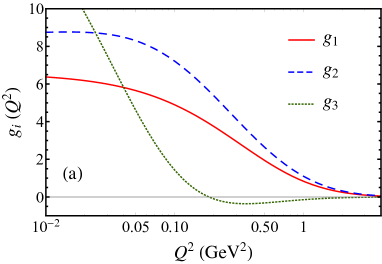
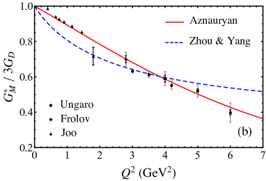
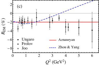
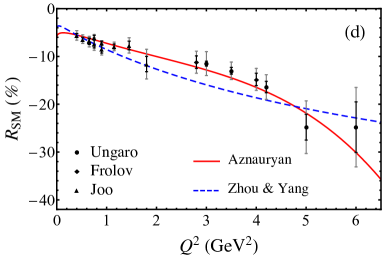
Figure 9: (a) $\gamma^{*}N\Delta$ transition form factors $g_{1}$, $g_{2}$ and $g_{3}$ versus $Q^{2}$, as used in this analysis Aznauryan and Burkert (2012); Aznauryan (2016); (b) magnetic $G_{M}^{*}$ form factor, scaled by the dipole form factor, $3\times G_{D}$; (c) electric to magnetic dipole ratio $R_{\rm EM}$ (in percent); and (d) Coulomb to magnetic dipole ratio $R_{\rm SM}$ (in percent). In (b), (c) and (d) the transition form factors from Aznauryan Aznauryan and Burkert (2012); Aznauryan (2016) (solid red curves) used in this analysis are compared with data from Ungaro et al. Ungaro et al. (2006) (circles), Frolov et al. Frolov et al. (1999) (diamonds), and Joo et al. Joo et al. (2002) (triangles), and with the recent parametrization by Zhou and Yang Zhou and Yang (2015).

The $\gamma^{*}N\Delta$ transition form factors $g_{1}$, $g_{2}$ and $g_{3}$ from the Eqs. (58)–(60) are illustrated in Fig. 9(a) as a function of $Q^{2}$. At moderate and large $Q^{2}$ values, $Q^{2}\gtrsim 0.1$ GeV², the $g_{1}$ and $g_{2}$ form factors dominate, with the $g_{3}$ form factor essentially zero. At very low $Q^{2}\lesssim 0.02$ GeV², the $g_{3}$ form factor rises rapidly and becomes larger than the largest contribution; for the phenomenological applications relevant to this paper, however, its role is essentially negligible.

The quality of the fit to the magnetic transition form factor $G_{M}^{*}$ is shown in Fig. 9(b), compared with data from several experiments Ungaro et al. (2006); Frolov et al. (1999); Joo et al. (2002) for $Q^{2}$ up to $\approx 6$ GeV². The parametrization in Eq. (58a) is compared with an alternative parametrization from the recent analysis by Zhou and Yang Zhou and Yang (2015), which agrees with the data in the intermediate $Q^{2}$ region, $Q^{2}\sim 3$–4 GeV², but underestimates (overestimates) the data at lower (higher) $Q^{2}$ values. Similarly, good agreement is obtained for the $R_{\rm EM}$ and $R_{\rm SM}$ ratios in Figs. 9(c) and 9(d), respectively, for the parametrizations in Eqs. (60) over the full range of $Q^{2}$ ($\lesssim 6$ GeV²) where data are available. The parametrization Zhou and Yang (2015) also agrees with the data at low $Q^{2}$ values, $Q^{2}\lesssim 1$ GeV², but discrepancies appear for larger $Q^{2}$.

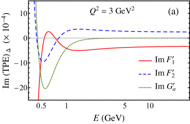
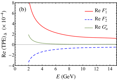
Figure 10: TPE contributions from $\Delta$ intermediate states to the (a) imaginary part and (b) real part of the generalized $F_{1}^{\prime}$ (solid red curves), $F_{2}^{\prime}$ (dashed blue curves) and $G_{a}^{\prime}$ (dotted black curves) form factors as a function of energy $E$, for fixed $Q^{2}=3$ GeV².

Using the Aznauryan parametrization Aznauryan and Burkert (2012); Aznauryan (2016) of the $\gamma^{*}N\Delta$ form factors, the TPE contributions from $\Delta$ intermediate states to the generalized form factors $F_{1}^{\prime}$, $F_{2}^{\prime}$ and $G_{a}^{\prime}$ are illustrated in Fig. 10 for both the imaginary and real parts. For the imaginary parts of the amplitudes, Fig. 10(a) shows resonance-like structure appearing in the unphysical region, $0.34<E<2$ GeV. As for the nucleon case, the unphysical region accounts for most of the dispersive integral, giving rise to smoothly decaying real parts of the amplitudes for $E\gtrsim 3$ GeV, as Fig. 10(b) illustrates.

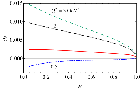
Figure 11: Dispersive TPE correction to the cross section, $\delta_{\Delta}$, from $\Delta$ intermediate states as a function of $\varepsilon$ for fixed values of $Q^{2}$ (= 0.5, 1, 2 and 3 GeV²).

As was observed in previous calculations of loop corrections Kondratyuk et al. (2005); Drell and Fubini (1959); Campbell (1969); Greenhut (1969), the contribution from $\Delta$ intermediate states, $\delta_{\Delta}$, is generally of opposite sign to the nucleon contribution $\delta_{N}$ for $Q^{2}\gtrsim 1$ GeV², and increases in magnitude with increasing $Q^{2}$, as Fig. 11 illustrates. Unlike previous loop calculations Kondratyuk et al. (2005); Zhou and Yang (2015), however, the correction $\delta_{\Delta}$ in the dispersive approach is well-behaved for all $\varepsilon$, vanishing in the $\varepsilon\to 1$ limit. In contrast, the correction $\delta_{\Delta}$ from the loop calculation with off-shell $\Delta$ states diverges as $\varepsilon\to 1$, as illustrated in Fig. 12(a). Note that the imaginary parts of the TPE amplitudes are identical for both calculations — only the real parts differ.

The nature of this divergence can be seen by plotting $\delta_{\Delta}$ versus electron energy $E$ instead of $\varepsilon$, as in Fig. 12(b). The linear divergence in $E$ indicates a violation of the Froissart bound Froissart (1961), and the breakdown of unitarity. This “pathological” behavior is not due to the inapplicability of hadronic models when $E\to\infty$ and $\varepsilon\to 1$, as suggested in Ref. Zhou and Yang (2015). Rather, it arises from an unphysical behavior of the off-shell contributions at high energies for interactions with derivative couplings.

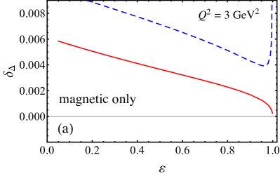
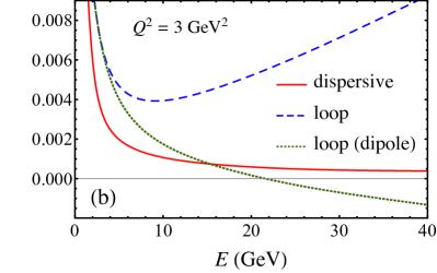
Figure 12: Comparison of the $\Delta$ intermediate state contribution to the TPE cross section, $\delta_{\Delta}$, for the dispersive (solid red curves) and loop (dashed blue curves) calculations at fixed $Q^{2}=3$ GeV²: (a) versus $\varepsilon$, and (b) versus electron energy $E$. Note that $\varepsilon=0.9$ corresponds to $E=5.9$ GeV for this $Q^{2}$. In (b) the loop corrections using a dipole approximation to the $\gamma^{*}N\Delta$ form factor with mass 0.75 GeV is also shown (dotted green curve). For simplicity only the dominant magnetic contribution has been considered.

As Fig. 12 illustrates, the loop calculations at large $\varepsilon$ are actually very sensitive to the shape of the $\gamma^{*}N\Delta$ form factors employed. Whether one use a dipole approximation or a more realistic parametrization, leads to significant differences with the dispersive approach already for $E\gtrsim 3$–4 GeV. (Here, for simplicity only the magnetic contribution to $\delta_{\Delta}$ is shown, but the effects are similar for the other $\gamma^{*}N\Delta$ form factors also.) In fact, the differences between the dispersive and loop calculations are significant not just near $\varepsilon\approx 1$, but also at lower $\varepsilon$ values. Generally, the magnitude of the dispersive $\Delta$ corrections is smaller than the loop results, resulting in less cancellation with the intermediate state nucleon contribution.

III.3 Verification of TPE effects

Having detailed the calculation of the TPE corrections from the nucleon and $\Delta$ intermediate states, we next compare the role of these corrections in observables that are particularly sensitive to effects beyond the Born approximation. These include the ratio of unpolarized $e^{+}p$ to $e^{-}p$ elastic scattering cross sections, and polarization transfer cross sections for longitudinally and transversely polarized electrons and protons.

III.3.1 $e^{+}p$ to $e^{-}p$ ratio

One of the observables that is most sensitive to the effects of TPE is the ratio of $e^{+}p$ to $e^{-}p$ elastic cross sections, which in the one-photon exchange approximation is unity. Since the TPE terms enter the $e^{+}p$ cross section with opposite sign to that in the $e^{-}p$ reaction, the ratio

$$R_{2\gamma} = \frac{\sigma^{e^{+}}}{\sigma^{e^{-}}}\ \approx\ 1-2\,\delta_{\gamma\gamma},$$ (61)

where $\sigma^{e^{\pm}}\equiv d\sigma({e^{\pm}p\to e^{\pm}p})/d\Omega$, provides a direct measure of effects beyond the Born approximation. Earlier data from elastic $e^{+}p$ and $e^{-}p$ experiments in the 1960s from SLAC Browman et al. (1965); Mar et al. (1968), Cornell Anderson et al. (1966), DESY Bartel et al. (1967) and Orsay Bouquet et al. (1968) gave some hints of a small enhancement of $R_{2\gamma}$ at forward angles and low $Q^{2}$, but were in the region (at large $\varepsilon$) where TPE is relatively small and were consistent within errors with $R_{2\gamma}=1$.

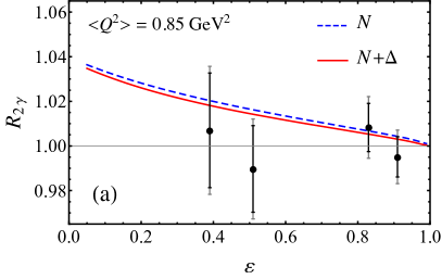
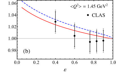
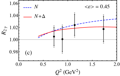
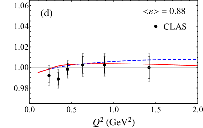
Figure 13: Ratio $R_{2\gamma}$ of $e^{+}p$ to $e^{-}p$ cross sections as a function of $\varepsilon$ for (a) fixed $\langle Q^{2}\rangle=0.85$ GeV² and (b) fixed $\langle Q^{2}\rangle=1.45$ GeV², and as a function of $Q^{2}$ for (c) fixed $\langle\varepsilon\rangle=0.45$ and (d) fixed $\langle\varepsilon\rangle=0.88$. The contributions with nucleon only (dashed blue curves) and the sum of nucleon and $\Delta$ (solid red curves) intermediate states are compared with data from CLAS at Jefferson Lab (circles) Rimal et al. (2016), with the statistical and systematic uncertainties indicated by the (black) inner and (gray) outer error bars, respectively.

More recently, several dedicated $e^{+}p$ to $e^{-}p$ ratio experiments have been performed in CLAS at Jefferson Lab Rimal et al. (2016), VEPP-3 in Novosibirsk Rachek et al. (2015); Nikolenko et al. (2014) and OLYMPUS at DESY Henderson et al. (1969) aimed at providing measurements of $R_{2\gamma}$ over a larger range of $\varepsilon$ and $Q^{2}$ with significantly reduced uncertainties. In Fig. 13 the $R_{2\gamma}$ ratio from the CLAS experiment is shown as a function of $\varepsilon$ at averaged $Q^{2}$ values of $\langle Q^{2}\rangle=0.85$ GeV² and $\langle Q^{2}\rangle=1.45$ GeV² [Figs. 13(a) and (b), respectively], and as a function of $Q^{2}$ at averaged $\varepsilon$ values of $\langle\varepsilon\rangle=0.45$ and $\langle\varepsilon\rangle=0.88$ GeV² [Figs. 13(c) and (d), respectively]. Most of the data at the larger $\varepsilon$ values are consistent with unity within the errors, but suggest a nonzero ratio, $\approx 2\%$ – 4% greater than unity, at the lowest $\varepsilon$ value for the higher-$Q^{2}$ set. The trend is consistent with the ratio calculated here, which shows a rising $R_{2\gamma}$ with decreasing $\varepsilon$. At these kinematics the calculated TPE correction is dominated by the nucleon elastic intermediate state, with the $\Delta$ contribution reducing the ratio slightly. Note that both the data and the calculated TPE corrections here (and elsewhere, unless otherwise stated) are shown relative to the Mo-Tsai infrared result.

The same trend is seen when the $R_{2\gamma}$ data are viewed as a function of $Q^{2}$ for fixed $\varepsilon$. At the larger average $\varepsilon$ value, $\langle\varepsilon\rangle=0.88$, the effects are consistent with zero as well as with the small predicted TPE correction. At the smaller value $\langle\varepsilon\rangle=0.45$, on the other hand, the larger predicted effect is consistent with the larger $R_{2\gamma}$ values with increasing $Q^{2}$. Again the effects of the $\Delta$ intermediate state are small at low $Q^{2}$ values, but become visible at larger $Q^{2}$, where they improve the agreement between the theory and experiment.

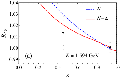
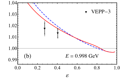
Figure 14: Ratio $R_{2\gamma}$ of $e^{+}p$ to $e^{-}p$ cross sections as a function of $\varepsilon$ for fixed energy (a) $E=1.594$ GeV and (b) $E=0.998$ GeV. The contributions with nucleon only (dashed blue curves) and the sum of nucleon and $\Delta$ (solid red curves) intermediate states are compared with data from the VEPP-3 experiment (triangles) Rachek et al. (2015), with the statistical and systematic uncertainties indicated by the (black) inner and (gray) outer error bars, respectively.

Data from the VEPP-3 experiment at Novosibirsk Rachek et al. (2015); Nikolenko et al. (2014), taken at energies $E\approx 1$ GeV and 1.6 GeV, are shown in Fig. 14 as a function of $\varepsilon$. The data correspond to a $Q^{2}$ range between $\approx 0.3$ GeV² and $\approx 1.5$ GeV², with $\varepsilon$ down to $\approx 0.3$. The ratio at the low $\varepsilon$ values shows an effect of magnitude 1% – 2%, slightly below but still consistent with the calculated TPE result at the $\approx 1\sigma$ level.

Most recently, the OLYMPUS experiment at DESY Henderson et al. (1969) measured the ratio $R_{2\gamma}$ at an energy $E=2.01$ GeV over a large range of $\varepsilon\sim 0.45-1$, corresponding to a $Q^{2}$ range from $\approx 0.2$ GeV² to 2 GeV². The results for the ratio $R_{2\gamma}$ are shown in Fig. 15. Interestingly, in contrast to the results from the CLAS and VEPP-3 experiments in Figs. 13 and 14, at large $\varepsilon$ values the trend in the data is towards values of the ratio slightly below unity, whereas the calculated dispersive TPE corrections give a ratio that has a small, $\lesssim 1\%$ enhancement above unity. At the lower $\varepsilon$ values, the trend is toward increasing values of $R_{2\gamma}$, consistent with the TPE calculation. Within the statistical and systematic uncertainties, including the overall normalization uncertainty of the OLYMPUS data, the theoretical result is consistent with the data over the entire $\varepsilon$ range. Note also that the $\lesssim 0.5\%$ correlated systematic (normalization) uncertainty quoted for the OLYMPUS data Henderson et al. (1969) is somewhat smaller than in the other $e^{+}p/e^{-}p$ experiments Rachek et al. (2015); Nikolenko et al. (2014).

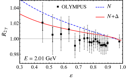
Figure 15: Ratio $R_{2\gamma}$ of $e^{+}p$ to $e^{-}p$ cross sections as a function of $\varepsilon$ for fixed energy $E=2.01$ GeV. The contributions with nucleon only (dashed blue curves) and the sum of nucleon and $\Delta$ (solid red curves) intermediate states are compared with data from the OLYMPUS experiment Henderson et al. (1969) (squares). The statistical and systematic uncertainties (correlated and uncorrelated) are indicated by the (black) inner and (gray) outer error bars, respectively.

While the possibility of unexpected effects in the high-$\varepsilon$ region is intriguing, we should note that the ratio $R_{2\gamma}$ defined in Ref. Henderson et al. (1969) is normalized by a ratio of $e^{+}$ to $e^{-}$ events obtained from a Monte Carlo (MC) simulation of the experiment designed to account for differences between electrons and positrons, $R_{2\gamma}\to(N_{\rm exp}^{e^{+}}/N_{\rm exp}^{e^{-}})/(N_{\rm MC}^{e^{+}}/N_{\rm MC}^{e^{-}})$. Here $N_{\rm exp}^{e^{\pm}}$ is the number of observed $e^{\pm}$ events, and $N_{\rm MC}^{e^{\pm}}$ is the number of simulated $e^{\pm}$ counts, taking into account radiative effects and various experimental settings. Of course, in order to simulate the elastic scattering cross sections, some input about the $e^{\pm}p$ interaction is needed for the MC, and it is possible that this may introduce additional model dependence into the procedure. Indeed, simulations using radiative corrections computed to order $\alpha^{3}$ versus those computed to all orders through exponentiation show that the latter can give $R_{2\gamma}$ values as much as 1% higher at the lowest $\varepsilon$ points Henderson et al. (1969). In Fig. 15 the results shown correspond to the ratio $R_{2\gamma}$ extracted with radiative corrections computed to all orders in $\alpha$.

The relatively large overall uncertainties on all of the currently available $R_{2\gamma}$ data unfortunately precludes any definitive conclusions about TPE effects that can be reached, other than that the effects are generally consistent with zero, as well as with the signs and magnitudes expected from the dispersive TPE calculations. This scenario calls for an urgent need for new measurements of $e^{+}p$ to $e^{-}p$ ratios at large $Q^{2}$, $Q^{2}\gtrsim 2$ GeV², and over a range of $\varepsilon$ values below $\varepsilon\sim 0.5$, where the TPE effects are predicted to be large enough ($\sim 2\%$) to be more clearly identified experimentally. On the other hand, the negative values of the slope in $\varepsilon$ predicted by the TPE calculations are generally consistent with the data from each of the CLAS Rimal et al. (2016), VEPP-3 Rachek et al. (2015); Nikolenko et al. (2014) and OLYMPUS Henderson et al. (1969) $e^{+}p/e^{-}p$ experiments.

III.3.2 Polarization observables

A complementary set of observables that can provide information on TPE effects involves polarization transfer in the elastic scattering of longitudinally polarized electrons from (unpolarized) protons, with measurement of the polarization of the final state proton, $\vec{e}p\to e\vec{p}$. Defining $P_{T}$ and $P_{L}$ to be the polarizations of recoil protons in the transverse and longitudinal directions relative to the proton momentum in the scattering plane, one has Guichon and Vanderhaeghen (2003)

$$P_{T} = -\frac{\sqrt{2\tau\varepsilon(1-\varepsilon)}}{\sigma_{R}}\Big{[}G_{E}G_{M}+G_{M}\operatorname{Re}\big{(}F_{1}^{\prime}-\tau F_{2}^{\prime}\big{)}+G_{E}\operatorname{Re}\big{(}F_{1}^{\prime}+F_{2}^{\prime}+\frac{\nu}{\tau}G_{a}^{\prime}\big{)}\Big{]},$$ (62a)

$$P_{L} = \frac{\tau\sqrt{1-\varepsilon^{2}}}{\sigma_{R}}\Big{[}G_{M}^{2}+2G_{M}\operatorname{Re}\big{(}F_{1}^{\prime}+F_{2}^{\prime}+\frac{\nu}{\tau(1+\varepsilon)}G_{a}^{\prime}\big{)}\Big{]},$$ (62b)

where $\sigma_{R}=\sigma_{R}^{\rm Born}(1+\delta_{{\gamma\gamma}})$, with the reduced Born cross section $\sigma_{R}^{\rm Born}$ given in Eq. (8), and $\delta_{{\gamma\gamma}}$ in Eq. (27). Note that the IR subtractions we have made in $F_{1}^{\prime}$ and $F_{2}^{\prime}$ are such that terms in the numerator and denominator of $P_{L}$ and $P_{T}$ cancel exactly, independent of regularization scheme. Taking the ratio of the transverse to longitudinal polarizations, we define

$$R_{TL} = -\mu_{p}\sqrt{\frac{\tau(1+\varepsilon)}{2\varepsilon}}\ \frac{P_{T}}{P_{L}}\,,$$ (63)

where $\mu_{p}$ is the proton’s magnetic moment. In the Born approximation, this reduces to a simple ratio of the electric to magnetic form factors, $R_{TL}\to\mu_{p}G_{E}/G_{M}$, which is a function only of $Q^{2}$ and is independent of $\varepsilon$.

The GEp2$\gamma$ experiment at Jefferson Lab Meziane et al. (2011) measured the ratios $R_{TL}$ and $P_{L}/P_{L}^{(0)}$, where $P_{L}^{(0)}$ is the Born level longitudinal polarization, at several values of $\varepsilon$ for fixed $Q^{2}=2.49$ GeV². These are shown in Fig. 16 as a function of $\varepsilon$, compared with the dispersive TPE calculations including nucleon and $\Delta$ intermediate states. The TPE effect on the longitudinal polarization ratio is very small, with the $P_{L}/P_{L}^{(0)}$ ratio only marginally below unity for all $\varepsilon$ values. Although the trend of the data suggests an increasing effect at high $\varepsilon$, the data are consistent with the TPE calculation if (correlated and uncorrelated) systematic uncertainties are taken into account.

The $\varepsilon$ dependence of the $R_{TL}$ ratio in Fig. 16 is also very weak, and in good agreement with the dispersive TPE calculation, especially once the $\Delta$ intermediate states are included. As for the $R_{2\gamma}$ ratio, higher-precision measurements of the polarization observables at larger $Q^{2}$ and lower $\varepsilon$ values would be valuable in more definitively identifying effects beyond the Born approximation.

Figure 16: (a) Ratio of the total longitudinal recoil proton polarization $P_{L}$ to the Born contribution $P_{L}^{(0)}$, and (b) ratio $R_{TL}$ of the transverse to longitudinal polarizations relative to the Born contribution, as a function of $\varepsilon$ for fixed $Q^{2}=2.49$ GeV². The dispersive calculation including nucleon only (dashed blue curves) and the sum of nucleon and $\Delta$ (solid red curves) intermediate states is compared with the data (circles) from the GEp2$\gamma$ experiment at Jefferson Lab Meziane et al. (2011), with the statistical and systematic (correlated and uncorrelated) uncertainties indicated by the (black) inner and (gray) outer error bars, respectively.

IV Outlook

In this paper we have presented a new approach to evaluating two-photon exchange effects in elastic electron–proton scattering, based on a dispersion relation analysis of the scattering amplitudes. We considered two methods for evaluating the imaginary parts of the loop diagrams, using analytic and numerical methods, and including the contributions from nucleon and $\Delta$ resonance intermediate states.

In contrast to previous calculations based on the direct evaluation of loop integrals, the dispersive analysis avoids uncertainties associated with off-shell intermediate states, and guarantees the correct behavior in the high energy limit. This problem is particularly egregious for the case of derivative interactions, such as for the $\Delta$ baryon, where the TPE amplitude in the off-shell calculation diverges linearly with energy in the forward limit. The dispersive approach, on the other hand, respects unitarity and is well-behaved at all energies.

The analytic dispersive method, which has been used recently in the literature Borisyuk and Kobushkin (2008, 2012, 2014, 2015); Tomalak and Vanderhaeghen (2015), has the advantage of allowing closed analytic expressions for the amplitudes in terms of simple logarithms, provided the vertex form factors can be parametrized in terms of sums or products of monopole functions. This has the virtue of increased speed of computation, but is limited by the accuracy of the monopole parametrization of the proton’s electric and magnetic form factors, which typically deteriorates markedly for $Q^{2}\gtrsim 5$–6 GeV².

The numerical contour method, in contrast, allows for a wide range of form factor parametrizations, and is relatively straightforward to implement. We find that in practice a simple contour is valid for any parametrization which has poles in the timelike region of $Q^{2}$. For more elaborate parametrizations that have with poles in the spacelike region, a special choice of contour can be used up to some maximum $Q^{2}$ that depends on the exact location of the poles.

To verify the utility of the dispersive approach, we have compared the results of the numerical TPE calculations with the most recent data on the ratio of $e^{+}p$ to $e^{-}p$ elastic scattering cross sections, which is directly sensitive to electromagnetic effects beyond the Born approximation. We find good agreement with the data from the CLAS Rimal et al. (2016) and VEPP-3 Rachek et al. (2015); Nikolenko et al. (2014) experiments. The results are also consistent, within the experimental uncertainties, with the more recent OLYMPUS experiment Henderson et al. (1969), which suggests a trend in the opposite direction at near-forward angles compared with the TPE calculations and the other data sets Rimal et al. (2016); Rachek et al. (2015); Nikolenko et al. (2014).

For the future, it will be important to extend the present framework to inelastic non-resonant intermediate states, including the $\pi N$ continuum, and allowing for widths of resonances. Efforts in this direction have been made recently in the literature Borisyuk and Kobushkin (2015); Tomalak et al. (2016), and will be aided by better knowledge of the empirical virtual Compton scattering amplitudes at non-forward angles. Beyond this, a longer term challenge is to further generalize the dispersive approach to higher $Q^{2}$ and intermediate state masses, merging the phenomenological hadronic description with one that expresses the TPE amplitudes explicitly in terms of partonic degrees of freedom.

On the experimental front, new, higher precision data on $e^{+}p$ and $e^{-}p$ cross sections at larger $Q^{2}$ values, $Q^{2}\gtrsim 3$ GeV², and lower $\varepsilon$ values, $\varepsilon\ll 1$, are needed to unambiguously identify TPE effects directly. The possibility of achieving this with a dedicated positron source at the 12 GeV Jefferson Lab facility remains an exciting prospect Arrington (2009). The technology described here for the TPE calculations can also be readily applied to the evaluation of $\gamma Z$ interference contributions in parity-violating electron–proton scattering, in the extraction of the strange electroweak form factors and the weak charge of the proton Arrington et al. (2011); Afanasev and Carlson (2005); Gorchtein and Horowitz (2009); Gorchtein et al. (2011); Rislow and Carlson (2011); Tjon et al. (2009); Sibirtsev et al. (2010); Hall et al. (2013, 2014, 2016).

Appendix A Generalized form factors

Beyond the Born approximation, the total amplitude for the elastic $ep\to ep$ scattering process can, for a massless electron, be decomposed into three independent amplitudes, or generalized form factors Guichon and Vanderhaeghen (2003). In this appendix we describe a practical method for extracting these generalized form factors from the total amplitude.

The objective is to map ${\cal M}_{{\gamma\gamma}}$ of Eq. (10) onto the generalized matrix element $\widehat{\cal M}_{\rm gen}(F_{1}^{\prime},F_{2}^{\prime},G_{a}^{\prime})$ given by Eq. (25),

$$\widehat{\cal M}_{\rm gen}(F_{1}^{\prime},F_{2}^{\prime},G_{a}^{\prime}) = -\frac{e^{2}}{q^{2}}\,\bar{u}_{e}(k^{\prime})\gamma_{\mu}u_{e}(k)\ \bar{u}_{N}(p^{\prime})\,\widehat{\Gamma}^{\mu}(F_{1}^{\prime},F_{2}^{\prime},0;q)\,u_{N}(p)$$ (64)

$$-\,\frac{e^{2}}{q^{2}}\,\bar{u}_{e}(k^{\prime})\gamma_{\mu}\gamma_{5}u_{e}(k)\ \bar{u}_{N}(p^{\prime})\,\widehat{\Gamma}^{\mu}(0,0,G_{a}^{\prime};q)\,u_{N}(p)\,,$$

where the generalized current operator $\widehat{\Gamma}^{\mu}$ is defined as

$$\widehat{\Gamma}^{\mu}(F_{1}^{\prime},F_{2}^{\prime},G_{a}^{\prime};q)=F_{1}^{\prime}(Q^{2},\nu)\,\gamma^{\mu}+F_{2}^{\prime}(Q^{2},\nu)\,\frac{i\sigma^{\mu\nu}q_{\nu}}{2M}+G_{a}^{\prime}(Q^{2},\nu)\gamma^{\mu}\gamma_{5}\,,$$ (65)

and the generalized form factors are functions of two variables, taken to be $Q^{2}$ and $\nu$.

The basic idea behind this method is to project $\widehat{\cal M}_{\rm gen}$ onto three linearly independent quantities (pseudo-observables) using Dirac trace techniques. The pseudo-observable projections are linear combinations of the amplitudes $F_{1}^{\prime}$, $F_{2}^{\prime}$, and $G_{a}^{\prime}$. The same projections are also made for ${\cal M}_{{\gamma\gamma}}$. One can then invert the transformation matrix to obtain $F_{1}^{\prime}$, $F_{2}^{\prime}$, and $G_{a}^{\prime}$ in terms of the pseudo-observable projections of ${\cal M}_{{\gamma\gamma}}$.

While any three linearly independent projections will suffice, it is convenient to use the same functional form given by $\widehat{\cal M}_{\rm gen}$. Consider the pseudo-observable

$$\sigma_{\rm gen} = \widehat{\cal M}_{\rm gen}^{\dagger}(A,B,C)\,\widehat{\cal M}_{\rm gen}(F_{1}^{\prime},F_{2}^{\prime},G_{a}^{\prime})$$ (66)

$$= Ax+By+Cz\,,$$

where $x$, $y$, and $z$ are linear combinations of $F_{1}^{\prime}$, $F_{2}^{\prime}$, and $G_{a}^{\prime}$, and $A$, $B$, and $C$ are placeholder coefficients representing the three independent projections. The overall factor $(-e^{2}/q^{2})^{2}$ is irrelevant for this derivation, and can be absorbed into the coefficients $\{A,B,C\}$. The expression for $\sigma_{\rm gen}$ can be obtained from

$$\sigma_{\rm gen}=L_{\alpha\mu}H^{\alpha\mu}\,,$$ (67)

where the leptonic and hadronic tensors are given by

$$L_{\alpha\mu} = \frac{1}{2}\operatorname{Tr}\left[\gamma_{\alpha}(\not{k}-\not{q})\gamma_{\mu}\not{k}\right]\,,$$ (68a)

$$H^{\alpha\mu} = \frac{1}{2}\operatorname{Tr}\biggl{[}\widehat{\Gamma}^{\alpha}(A,B,C;-q)(\not{p}+\not{q}+M)\widehat{\Gamma}^{\mu}(F_{1}^{\prime},F_{2}^{\prime},G_{a}^{\prime};q)(\not{p}+M)\biggr{]}\,,$$ (68b)

respectively. Note that rather than keeping the vector and axial-vector terms separate, we have combined them into one compact expression. This is possible because the parity-violating terms in the combined amplitude vanish after taking the traces. Evaluating the traces, one finds

$$\sigma_{\rm gen}=(A,B,C)\cdot\left(\begin{array}[]{c}x\\ y\\ z\end{array}\right)=(A,B,C)\cdot\mathbb{M}\cdot\left(\begin{array}[]{c}F_{1}^{\prime}\\ F_{2}^{\prime}\\ G_{a}^{\prime}\end{array}\right)\,,$$ (69)

where the transformation matrix $\mathbb{M}$ is given by

$$\mathbb{M}=16M^{4}\left(\begin{array}[]{ccc}\nu^{2}+\tau^{2}-\tau&2\tau^{2}&2\nu\tau\\ 2\tau^{2}&\tau\left(\nu^{2}-\tau^{2}+\tau\right)&2\nu\tau\\ 2\nu\tau&2\nu\tau&\nu^{2}+\tau^{2}+\tau\\ \end{array}\right)\,.$$ (70)

Inverting the matrix $\mathbb{M}$ will obtain the relationships of interest,

$$\left(\begin{array}[]{c}F_{1}^{\prime}\\ F_{2}^{\prime}\\ G_{a}^{\prime}\end{array}\right) = \frac{1}{16M^{4}\left(\nu^{2}-\tau(\tau+1)\right)^{2}}\$$ (81)

$$\times\left(\begin{array}[]{ccc}\nu^{2}+\tau^{2}-\tau&2\tau&-2\nu\tau\\ 2\tau&(\nu^{2}-\tau^{2}+\tau)/\tau&-2\nu\\ -2\nu\tau&-2\nu&\nu^{2}+\tau^{2}+\tau\\ \end{array}\right)\left(\begin{array}[]{c}x\\ y\\ z\end{array}\right).$$

The same projections as in Eq. (66) can now be made for ${\cal M}_{{\gamma\gamma}}$,

$$\sigma_{\rm gen} = \widehat{\cal M}_{\rm gen}^{\dagger}(A,B,C)\,{\cal M}_{{\gamma\gamma}}$$ (82)

$$= Ax+By+Cz\,.$$

The set of projected functions $\left\{x,y,z\right\}$ are then combined to give the TPE amplitudes using Eq. (81). There is an apparent kinematic singularity in Eq. (81) at $\nu^{2}=\tau(\tau+1)=\nu_{\rm ph}^{2}$, which is the threshold between the physical and unphysical regions. However, the full expressions for the imaginary parts of $F_{1}^{\prime}(Q^{2},\nu)$, $F_{2}^{\prime}(Q^{2},\nu)$, and $G_{a}^{\prime}(Q^{2},\nu)$ are continuous, smooth, and finite across this boundary. Nevertheless, for numerical work we avoid directly using this kinematic point.

From Eq. (10), the pseudo-observable $\sigma_{\rm gen}$ has the form

$$\sigma_{\rm gen}=\frac{\alpha}{4\pi}Q^{2}\frac{1}{i\pi^{2}}\int d^{4}q_{1}\ \frac{L_{\alpha\mu\nu}H^{\alpha\mu\nu}}{(q_{1}^{2}-\lambda^{2})(q_{2}^{2}-\lambda^{2})}\,,$$ (83)

where the leptonic and hadronic tensors of Eq. (11)–(12) are

$$L_{\alpha\mu\nu} = \frac{1}{2}\operatorname{Tr}\left[\gamma_{\alpha}(1+\gamma_{5})(\not{k}-\not{q})\gamma_{\mu}S_{F}(k-q_{1})\gamma_{\nu}\not{k}\right]\,,$$ (84)

$$H^{\alpha\mu\nu} = \frac{1}{2}\operatorname{Tr}\biggl{[}\widehat{\Gamma}^{\alpha}(A,B,C;-q)(\not{p}+\not{q}+M)$$ (85)

$$\hskip 14.22636pt\times\ \Gamma_{R\to N\gamma}^{\mu\lambda}(p+q_{1},-q_{2})\,S_{\lambda\rho}(p+q_{1},M_{R})\,\Gamma_{\gamma N\to R}^{\rho\nu}(p+q_{1},q_{1})(\not{p}+M)\biggr{]}\,.$$

The decomposition of the total amplitude into a basis of generalized form factors is not unique. Another convention in the literature Chen et al. (2004); Tomalak and Vanderhaeghen (2015) is to use the generalized matrix element

$$\widetilde{\cal M}_{\rm gen}(\widetilde{F}_{1},\widetilde{F}_{2},\widetilde{F}_{3}) = -\frac{e^{2}}{q^{2}}\,\bar{u}_{e}(k^{\prime})\gamma_{\mu}u_{e}(k)$$

$$\times\ \bar{u}_{N}(p^{\prime})\biggl{[}\widetilde{F}_{1}(Q^{2},\nu)\,\gamma^{\mu}+\widetilde{F}_{2}(Q^{2},\nu)\,\frac{i\sigma^{\mu\nu}q_{\nu}}{2M}+\widetilde{F}_{3}(Q^{2},\nu)\frac{\not{k}\,p^{\mu}}{M^{2}}\biggr{]}u_{N}(p)\,,$$

The relationship between the set $\{F_{1}^{\prime},F_{2}^{\prime},G_{a}^{\prime}\}$ and the set $\{\widetilde{F}_{1},\widetilde{F}_{2},\widetilde{F}_{3}\}$ is $F_{1}^{\prime}=\widetilde{F}_{1}+\nu\widetilde{F}_{3}$, $F_{2}^{\prime}=\widetilde{F}_{2}$, and $G_{a}^{\prime}=-\tau\widetilde{F}_{3}$ Chen et al. (2004). This relationship can be easily derived by contracting $\widetilde{\cal M}_{\rm gen}$ with $\widehat{\cal M}_{\rm gen}^{\dagger}$, in analogy with Eq. (66), and comparing the transformation matrices.

Appendix B Analytic expressions for imaginary parts of Passarino-Veltman functions

In the notation of the LoopTools package Hahn and Perez-Victoria (1999), the full dependence of the $s$-channel PV functions on kinematic variables is

$$B_{0}(s) \equiv B_{0}(s;m_{e},W)\,,$$ (87a)

$$C_{0}(s;\Lambda) \equiv C_{0}(M^{2},m_{e}^{2},s;W,\Lambda,m_{e})\,,$$ (87b)

$$D_{0}(s;\Lambda_{1},\Lambda_{2}) \equiv D_{0}(M^{2},M^{2},m_{e}^{2},m_{e}^{2},t,s;\Lambda_{1},W,\Lambda_{2},m_{e})\,.$$ (87c)

Following the discussion in Sec. II.2.1, the full expressions for the imaginary parts of the these functions are

$$b_{0}(s) = \frac{\pi s_{W}}{s}\,\theta(s_{W})\,,$$ (88a)

$$c_{0}(s;\Lambda) = -\frac{\pi}{s_{M}}\log\left(\frac{\Lambda^{2}s+s_{M}s_{W}}{s\Lambda^{2}}\right)\,\theta(s_{W})\,,$$ (88b)

$$d_{0}(s;\Lambda_{1},\Lambda_{2}) = \frac{s_{W}}{4s}J\,\theta(s_{W})\,,$$ (88c)

where $s_{M}$ and $s_{W}$ are given by Eq. (34), the quantity $J$ is given by

$$J = \frac{4\pi}{Y\sqrt{1-z^{2}}}\log\left(\frac{1+\sqrt{1-z^{2}}}{z}\right)\,,$$ (89)

and we have introduced the dimensionless variable $z=Z/Y$, with

$$Z = \frac{\Lambda_{1}\Lambda_{2}\sqrt{(\Lambda_{1}^{2}s+s_{M}s_{W})(\Lambda_{2}^{2}s+s_{M}s_{W})}}{s}\,,$$ (90)

$$Y = \frac{2\Lambda_{1}^{2}\Lambda_{2}^{2}s+s_{M}s_{W}\left(\Lambda_{1}^{2}+\Lambda_{2}^{2}\right)+Q^{2}s_{W}^{2}}{2s}\,.$$ (91)

The expression for $d_{0}(s;\Lambda_{1},\Lambda_{2})$ in Eq. (88c) has been rewritten in a form that is numerically stable for very small values of $\Lambda_{i}$. By comparison, the form given in Eq. (37), with $X^{2}=Y^{2}-Z^{2}$, is susceptible to roundoff error in this limit. We also note that while the real part of $D_{0}$ has a logarithmic dependence on $m_{e}$, the imaginary part does not, and is therefore finite in the limit $m_{e}\to 0$, which we have used throughout this paper.

The PV functions $c_{0}(s;\Lambda)$ and $d_{0}(s;\Lambda_{1},\Lambda_{2})$ are IR-divergent in the limit $\Lambda^{2}\to 0$. Replacing $\Lambda^{2}\to\lambda^{2}$, and keeping only logarithmic terms in $\lambda^{2}$, we have the three IR-divergent combinations

$$c_{0}(s;\lambda) = -\frac{\pi}{s_{M}}\log\left(\frac{s_{M}s_{W}}{\lambda^{2}s}\right)\,\theta(s_{W})\,,$$ (92a)

$$d_{0}(s;\lambda,\Lambda) = \frac{\pi}{\Lambda^{2}s_{M}+Q^{2}s_{W}}\log\left(\frac{s_{W}\left(\Lambda^{2}s_{M}+Q^{2}s_{W}\right)^{2}}{\lambda^{2}\Lambda^{2}s_{M}\left(\Lambda^{2}s+s_{M}s_{W}\right)}\right)\,\theta(s_{W})\,,$$ (92b)

$$d_{0}(s;\lambda,\lambda) = \frac{2\pi}{Q^{2}s_{W}}\log\left(\frac{Q^{2}s_{W}}{\lambda^{2}s_{M}}\right)\,\theta(s_{W})\,.$$ (92c)

One can use these expressions to explicitly show that there is no residual dependence on $\lambda$ in the total TPE amplitudes, after subtracting the model-independent Maximon and Tjon IR-divergent terms. For numerical calculations, it is more convenient to use the full expressions (88), with a value for $\lambda$ satisfying the criterion $\lambda^{2}\ll m_{e}^{2}$.

Table 1: Table of values for $I_{ij}$ in Eq. (42), keeping only logarithmic terms in the infinitesimal regulator $\lambda$. The dependence on $s$ and other kinematic variables is suppressed for clarity.

$N$	$i$	$j$	$I_{ij}$
0	0	0	$d_{0}(\lambda,\lambda)-d_{0}(\Lambda_{1},\lambda)-d_{0}(\lambda,\Lambda_{2})+d_{0}(\Lambda_{1},\Lambda_{2})$
1	1	0	$\Lambda_{1}^{2}\left(d_{0}(\Lambda_{1},\lambda)-d_{0}(\Lambda_{1},\Lambda_{2})\right)$
1	0	1	$\Lambda_{2}^{2}\left(d_{0}(\lambda,\Lambda_{2})-d_{0}(\Lambda_{1},\Lambda_{2})\right)$
2	2	0	$-\Lambda_{1}^{2}\left(c_{0}(\lambda)-c_{0}(\Lambda_{2})+\Lambda_{1}^{2}\left(d_{0}(\Lambda_{1},\lambda)-d_{0}(\Lambda_{1},\Lambda_{2})\right)\right)$
2	0	2	$-\Lambda_{2}^{2}\left(c_{0}(\lambda)-c_{0}(\Lambda_{1})+\Lambda_{2}^{2}\left(d_{0}(\lambda,\Lambda_{2})-d_{0}(\Lambda_{1},\Lambda_{2})\right)\right)$
2	1	1	$\Lambda_{1}^{2}\Lambda_{2}^{2}d_{0}(\Lambda_{1},\Lambda_{2})$

For sums of monopole form factors, the integrals of interest are sums of primitive integrals $I_{ij}$ given in Eq. (42), with $N=i+j$. Table 1 gives the values for $I_{ij}$ up to $N=2$, which suffices for nucleon intermediate states. In general, for other states like the $\Delta$ one needs up to $N=3$, which requires the form factor to behave like $1/Q_{i}^{4}$ asymptotically, but the procedure follows analogously.

Appendix C Form factor reparametrizations

Here we present the reparametrizations of the nucleon and $\Delta$ vertex form factors in terms of sums and/or products of monopoles, suitable for use in the analytic expressions of Sec. II.2.1. Fits are over the range $0<Q^{2}<8$ GeV², with $F_{1}(Q^{2})$ being a 5-parameter fit, while all others are 4-parameter fits.

The nucleon form factors are fit to the parametrization of Ref. Venkat et al. (2011),

$$F_{1}(Q^{2}) = \frac{0.334}{1+Q^{2}/0.209}+\frac{1.228}{1+Q^{2}/0.805}-\frac{0.562}{1+Q^{2}/1.898}\,,$$ (93)

$$F_{2}(Q^{2}) = \frac{\kappa}{1+Q^{2}/3.502}\left(\frac{1.165}{1+Q^{2}/0.364}-\frac{0.165}{1+Q^{2}/2.675}\right)\,,$$ (94)

with $Q^{2}$ in GeV². Defining

$$g(Q^{2})=\frac{(M_{\Delta}+M)^{2}}{Q_{+}^{2}}=\frac{1}{1+Q^{2}/(M_{\Delta}+M)^{2}}\,,$$ (95)

the $\Delta$ transition form factors are fit to the parametrization of Ref. Aznauryan and Burkert (2012); Aznauryan (2016),

$$g(Q^{2})\,G_{M,E}^{*}(Q^{2}) = G_{M,E}^{*}(0)\frac{1}{1+Q^{2}/3.177}\left(\frac{2.474}{1+Q^{2}/0.575}-\frac{1.474}{1+Q^{2}/1.000}\right)\,,$$ (96)

$$g(Q^{2})\,G_{C}^{*}(Q^{2}) = G_{C}^{*}(0)\frac{1}{\left(1+Q^{2}/1.102\right)^{2}}\left(\frac{0.813}{1+Q^{2}/0.0684}+\frac{0.187}{1+Q^{2}/0.895}\right)\,.$$ (97)

The form factors $g_{1}(Q^{2})$, $g_{2}(Q^{2})$, and $g_{3}(Q^{2})$ can be obtained from simple combinations of these parametrizations, while still allowing for implementation in analytic form.

The use of these reparametrizations in the numerical integration method allows for a test of our codes against the analytic results. We were routinely able to obtain a relative agreement at the level of five significant digits. Similarly, the validity of using these reparametrizations in the analytic codes can be tested against the numerical results using the original functional forms. In general, we found that the relative differences between the analytic and numerical evaluations of the imaginary parts of the TPE amplitudes were comparable to the relative differences between the original and reparametrized forms over the relevant range of $Q^{2}$. As the original and reparametrized vertex form factors given in this appendix agree at roughly the 2% level when averaged over the range $0<Q^{2}<8$ GeV², we find a 2% agreement in $F_{1}^{\prime}(Q^{2},\nu)$, $F_{2}^{\prime}(Q^{2},\nu)$, and $G_{a}^{\prime}(Q^{2},\nu)$ up to $Q^{2}=4$ GeV². This suggests that the TPE results are not very sensitive to pole structure of the vertex form factor parametrizations in the complex plane.

References

- Hofstadter and McAllister (1955) R. Hofstadter and R. W. McAllister, Phys. Rev. 98, 217 (1955).
- Jones et al. (2000) M. K. Jones et al., Phys. Rev. Lett. 84, 1398 (2000), eprint nucl-ex/9910005.
- Gayou et al. (2002) O. Gayou et al., Phys. Rev. Lett. 88, 092301 (2002), eprint nucl-ex/0111010.
- Blunden et al. (2003) P. G. Blunden, W. Melnitchouk, and J. A. Tjon, Phys. Rev. Lett. 91, 142304 (2003), eprint nucl-th/0306076.
- Guichon and Vanderhaeghen (2003) P. A. M. Guichon and M. Vanderhaeghen, Phys. Rev. Lett. 91, 142303 (2003), eprint hep-ph/0306007.
- Tsai (1961) Y.-S. Tsai, Phys. Rev. 122, 1898 (1961).
- Mo and Tsai (1969) L. W. Mo and Y.-S. Tsai, Rev. Mod. Phys. 41, 205 (1969).
- Kondratyuk et al. (2005) S. Kondratyuk, P. G. Blunden, W. Melnitchouk, and J. A. Tjon, Phys. Rev. Lett. 95, 172503 (2005), eprint nucl-th/0506026.
- Blunden et al. (2005) P. G. Blunden, W. Melnitchouk, and J. A. Tjon, Phys. Rev. C72, 034612 (2005), eprint nucl-th/0506039.
- Kondratyuk and Blunden (2007) S. Kondratyuk and P. G. Blunden, Phys. Rev. C75, 038201 (2007), eprint nucl-th/0701003.
- Nagata et al. (2009) K. Nagata, H. Q. Zhou, C. W. Kao, and S. N. Yang, Phys. Rev. C79, 062501 (2009), eprint arXiv:0811.3539.
- Graczyk (2013) K. M. Graczyk, Phys. Rev. C88, 065205 (2013), eprint arXiv:1306.5991.
- Lorenz et al. (2015) I. T. Lorenz, U.-G. Meissner, H. W. Hammer, and Y. B. Dong, Phys. Rev. D91, 014023 (2015), eprint arXiv:1411.1704.
- Zhou and Yang (2015) H.-Q. Zhou and S. N. Yang, Eur. Phys. J. A51, 105 (2015), eprint arXiv:1407.2711.
- Zhou (2017) H.-Q. Zhou, Phys. Rev. C95, 025203 (2017), eprint arXiv:1610.05957.
- Chen et al. (2004) Y. C. Chen, A. Afanasev, S. J. Brodsky, C. E. Carlson, and M. Vanderhaeghen, Phys. Rev. Lett. 93, 122301 (2004), eprint hep-ph/0403058.
- Afanasev et al. (2005) A. V. Afanasev, S. J. Brodsky, C. E. Carlson, Y.-C. Chen, and M. Vanderhaeghen, Phys. Rev. D72, 013008 (2005), eprint hep-ph/0502013.
- Gorchtein (2007) M. Gorchtein, Phys. Lett. B644, 322 (2007), eprint hep-ph/0610378.
- Borisyuk and Kobushkin (2008) D. Borisyuk and A. Kobushkin, Phys. Rev. C78, 025208 (2008), eprint arXiv:0804.4128.
- Borisyuk and Kobushkin (2015) D. Borisyuk and A. Kobushkin, Phys. Rev. C92, 035204 (2015), eprint arXiv:1506.02682.
- Tomalak and Vanderhaeghen (2015) O. Tomalak and M. Vanderhaeghen, Eur. Phys. J. A51, 24 (2015), eprint arXiv:1408.5330.
- Carlson and Vanderhaeghen (2007) C. E. Carlson and M. Vanderhaeghen, Ann. Rev. Nucl. Part. Sci. 57, 171 (2007), eprint hep-ph/0701272.
- Arrington et al. (2011) J. Arrington, P. G. Blunden, and W. Melnitchouk, Prog. Part. Nucl. Phys. 66, 782 (2011), eprint arXiv:1105.0951.
- Afanasev et al. (2017) A. Afanasev, P. G. Blunden, D. Hasell, and B. A. Raue, Prog. Part. Nucl. Phys. (2017).
- Rimal et al. (2016) D. Rimal et al. (2016), eprint arXiv:1603.00315.
- Rachek et al. (2015) I. A. Rachek et al., Phys. Rev. Lett. 114, 062005 (2015), eprint arXiv:1411.7372.
- Nikolenko et al. (2014) D. M. Nikolenko et al., EPJ Web Conf. 66, 06002 (2014).
- Henderson et al. (1969) B. S. Henderson et al., Phys. Rev. Lett. 118, 092501 (1969), eprint arXiv:1611.04685.
- Borisyuk and Kobushkin (2012) D. Borisyuk and A. Kobushkin, Phys. Rev. C86, 055204 (2012), eprint arXiv:1206.0155.
- Borisyuk and Kobushkin (2014) D. Borisyuk and A. Kobushkin, Phys. Rev. C89, 025204 (2014), eprint arXiv:1306.4951.
- Meziane et al. (2011) M. Meziane et al., Phys. Rev. Lett. 106, 132501 (2011), eprint arXiv:1012.0339.
- ’t Hooft and Veltman (1979) G. ’t Hooft and M. J. G. Veltman, Nucl. Phys. B153, 365 (1979).
- Passarino and Veltman (1979) G. Passarino and M. J. G. Veltman, Nucl. Phys. B160, 151 (1979).
- Mertig et al. (1991) R. Mertig, M. Bohm, and A. Denner, Comput. Phys. Commun. 64, 345 (1991).
- Shtabovenko et al. (2016) V. Shtabovenko, R. Mertig, and F. Orellana, Comput. Phys. Commun. 207, 432 (2016), eprint arXiv:1601.01167.
- Hahn and Perez-Victoria (1999) T. Hahn and M. Perez-Victoria, Comput. Phys. Commun. 118, 153 (1999), eprint hep-ph/9807565.
- Grammer and Yennie (1973) G. Grammer, Jr. and D. R. Yennie, Phys. Rev. D8, 4332 (1973).
- Maximon and Tjon (2000) L. C. Maximon and J. A. Tjon, Phys. Rev. C62, 054320 (2000), eprint nucl-th/0002058.
- Tomalak and Vanderhaeghen (2014) O. Tomalak and M. Vanderhaeghen, Phys. Rev. D90, 013006 (2014), eprint arXiv:1405.1600.
- Tjon and Melnitchouk (2008) J. A. Tjon and W. Melnitchouk, Phys. Rev. Lett. 100, 082003 (2008), eprint arXiv:0711.0143.
- Tjon et al. (2009) J. A. Tjon, P. G. Blunden, and W. Melnitchouk, Phys. Rev. C79, 055201 (2009), eprint arXiv:0903.2759.
- van Hameren (2011) A. van Hameren, Comput. Phys. Commun. 182, 2427 (2011), eprint arXiv:1007.4716.
- Carrazza et al. (2016) S. Carrazza, R. K. Ellis, and G. Zanderighi, Comput. Phys. Commun. 209, 134 (2016), eprint arXiv:1605.03181.
- Denner et al. (2017) A. Denner, S. Dittmaier, and L. Hofer, Comput. Phys. Commun. 212, 220 (2017), eprint arXiv:1604.06792.
- Cutkosky (1958) R. E. Cutkosky, Phys. Rev. 112, 1027 (1958).
- Mandelstam (1958) S. Mandelstam, Phys. Rev. 112, 1344 (1958).
- Beenakker and Denner (1990) W. Beenakker and A. Denner, Nucl. Phys. B338, 349 (1990).
- Kelly (2004) J. J. Kelly, Phys. Rev. C70, 068202 (2004).
- Arrington et al. (2007) J. Arrington, W. Melnitchouk, and J. A. Tjon, Phys. Rev. C76, 035205 (2007), eprint arXiv:0707.1861.
- Venkat et al. (2011) S. Venkat, J. Arrington, G. A. Miller, and X. Zhan, Phys. Rev. C83, 015203 (2011), eprint arXiv:1010.3629.
- Gorchtein and Horowitz (2008) M. Gorchtein and C. J. Horowitz, Phys. Rev. C77, 044606 (2008), eprint nucl-th/0801.4575.
- Bernauer et al. (2010) J. C. Bernauer et al., Phys. Rev. Lett. 105, 242001 (2010), eprint arXiv:1007.5076.
- Kelly (2002) J. J. Kelly, Phys. Rev. C66, 065203 (2002), eprint hep-ph/0204239.
- Bosted (1995) P. E. Bosted, Phys. Rev. C51, 409 (1995).
- Brash et al. (2002) E. J. Brash, A. Kozlov, S. Li, and G. M. Huber, Phys. Rev. C65, 051001 (2002), eprint hep-ex/0111038.
- Jones and Scadron (1973) H. F. Jones and M. D. Scadron, Annals Phys. 81, 1 (1973).
- Pascalutsa et al. (2007) V. Pascalutsa, M. Vanderhaeghen, and S. N. Yang, Phys. Rept. 437, 125 (2007), eprint hep-ph/0609004.
- Pascalutsa and Tjon (2004) V. Pascalutsa and J. A. Tjon, Phys. Rev. C70, 035209 (2004), eprint nucl-th/0407068.
- Caia et al. (2004) G. L. Caia, V. Pascalutsa, J. A. Tjon, and L. E. Wright, Phys. Rev. C70, 032201 (2004), eprint nucl-th/0407069.
- Aznauryan and Burkert (2012) I. G. Aznauryan and V. D. Burkert, Prog. Part. Nucl. Phys. 67, 1 (2012), eprint arXiv:1109.1720.
- Aznauryan (2016) I. G. Aznauryan, private communication (2016).
- Ungaro et al. (2006) M. Ungaro et al., Phys. Rev. Lett. 97, 112003 (2006), eprint hep-ex/0606042.
- Frolov et al. (1999) V. V. Frolov et al., Phys. Rev. Lett. 82, 45 (1999), eprint hep-ex/9808024.
- Joo et al. (2002) K. Joo et al., Phys. Rev. Lett. 88, 122001 (2002), eprint hep-ex/0110007.
- Drell and Fubini (1959) S. D. Drell and S. Fubini, Phys. Rev. 113, 741 (1959).
- Campbell (1969) J. A. Campbell, Phys. Rev. 180, 1541 (1969).
- Greenhut (1969) G. K. Greenhut, Phys. Rev. 184, 1860 (1969).
- Froissart (1961) M. Froissart, Phys. Rev. 123, 1053 (1961).
- Browman et al. (1965) A. Browman, F. Liu, and C. Schaerf, Phys. Rev. 139, B1079 (1965).
- Mar et al. (1968) J. Mar, B. C. Barish, J. Pine, D. H. Coward, H. C. DeStaebler, J. Litt, A. Minten, R. E. Taylor, and M. Breidenbach, Phys. Rev. Lett. 21, 482 (1968).
- Anderson et al. (1966) R. L. Anderson, B. Borgia, G. L. Cassiday, J. W. DeWire, A. S. Ito, and E. C. Loh, Phys. Rev. Lett. 17, 407 (1966).
- Bartel et al. (1967) W. Bartel, B. Dudelzak, H. Krehbiel, J. M. McElroy, R. J. Morrison, W. Schmidt, V. Walther, and G. Weber, Phys. Lett. B25, 242 (1967).
- Bouquet et al. (1968) B. Bouquet, D. Benaksas, B. Grossetête, B. Jean-Marie, G. Parrour, J. P. Poux, and R. Tchapoutian, Phys. Lett. B26, 178 (1968).
- Tomalak et al. (2016) O. Tomalak, B. Pasquini, and M. Vanderhaeghen (2016), eprint arXiv:1612.07726.
- Arrington (2009) J. Arrington, AIP Conf. Proc. 1160, 13 (2009), eprint arXiv:0905.0713.
- Afanasev and Carlson (2005) A. V. Afanasev and C. E. Carlson, Phys. Rev. Lett. 94, 212301 (2005), eprint hep-ph/0502128.
- Gorchtein and Horowitz (2009) M. Gorchtein and C. J. Horowitz, Phys. Rev. Lett. 102, 091806 (2009), eprint arXiv:0811.0614.
- Gorchtein et al. (2011) M. Gorchtein, C. J. Horowitz, and M. J. Ramsey-Musolf, Phys. Rev. C84, 015502 (2011), eprint arXiv:1102.3910.
- Rislow and Carlson (2011) B. C. Rislow and C. E. Carlson, Phys. Rev. D83, 113007 (2011), eprint arXiv:1011.2397.
- Sibirtsev et al. (2010) A. Sibirtsev, P. G. Blunden, W. Melnitchouk, and A. W. Thomas, Phys. Rev. D82, 013011 (2010), eprint arXiv:1002.0740.
- Hall et al. (2013) N. L. Hall, P. G. Blunden, W. Melnitchouk, A. W. Thomas, and R. D. Young, Phys. Rev. D88, 013011 (2013), eprint arXiv:1304.7877.
- Hall et al. (2014) N. L. Hall, P. G. Blunden, W. Melnitchouk, A. W. Thomas, and R. D. Young, Phys. Lett. B731, 287 (2014), [Erratum: Phys. Lett.B733,380(2014)], eprint arXiv:1311.3389.
- Hall et al. (2016) N. L. Hall, P. G. Blunden, W. Melnitchouk, A. W. Thomas, and R. D. Young, Phys. Lett. B753, 221 (2016), eprint arXiv:1504.03973.